Embed Size (px)
Citation preview

Draft
Integrated System of Equations for Estimating Stem
Volume, Density and Biomass for Australian Red Cedar Plantation
Journal: Canadian Journal of Forest Research
Manuscript ID cjfr-2016-0135.R3
Manuscript Type: Article
Date Submitted by the Author: 20-Jan-2017
Complete List of Authors: Calegario, Natalino; Federal University of Lavras, Forestry
Gregoire, Timothy; Yale University Silva, Tatiane; Universidade Federal de Lavras, Forestry Tomazello Filho, Mario; University of Sao Paulo, Department of Forest Sciences Alves, Joyce; Universidade Federal de Lavras
Keyword: Wood density, </i>Toona ciliata</i>, System of equations, Wood Technology, biomass estimation
https://mc06.manuscriptcentral.com/cjfr-pubs
Canadian Journal of Forest Research

Draft
1
Integrated system of equations for estimating stem volume, density and biomass 1
for Australian red cedar plantations 2
Natalino Calegario, School of Forestry and Environmental Studies, Yale University, 3
New Haven, CT 06511, USA. (e-mail: [email protected]) 4
Timothy G. Gregoire, School of Forestry and Environmental Studies, Yale University, 5
New Haven, CT 06511, USA. (e-mail: [email protected]) 6
Tatiane Antunes da Silva, Department of Forest Science, Federal University of Lavras, 7
Lavras, MG 37200, Brazil. (e-mail: [email protected]) 8
Mario Tomazello Filho, Department of Forest Sciences, College of Agriculture “Luiz de 9
Queiroz”, University of São Paulo, Piracicaba, 13418, Sao Paulo, Brazil (e-mail: 10
Joyce A. Alves. Department of Forest Science, Federal University of Lavras, Lavras, 12
MG 37200, Brazil. (e-mail: [email protected]) 13
Corresponding author. Name: Natalino Calegario; e-mail: [email protected]; Phone: 1 14
203-219-1052; Mail: 195 Prospect Street, Yale University, New Haven, CT, USA 15
06511. 16
17
18
19
20
21
22
23
24
25
Page 1 of 33
https://mc06.manuscriptcentral.com/cjfr-pubs
Canadian Journal of Forest Research

Draft
2
Abstract 26
A system of equations is proposed to assess the stem wood density variation of Toona 27
ciliata M. Roem. stems growing in Brazilian plantations. As a taper function, a 3-degree 28
polynomial was fitted and the stem radius squared (r2), the dependent variable, was 29
estimated as a function of diameter at breast height (dbh), total height (ht) and radius (r) 30
at height (h). A nonlinear function was fitted to estimate wood density variation, having 31
as the independent variable the ratio between radius r and height h. The stem mass was 32
estimated by integrating the product of stem volume and wood density. Stem 33
measurements from a group of 72 trees of Toona ciliata M. Roem. were used to fit the 34
taper equation. A group of 6 trees was selected and, using x-ray technology, a wood 35
density database was created. Both the taper and the nonlinear functions performed well 36
in estimating the radius and the wood density. The within tree wood density 37
systematically increased from pith to bark and from the base to the top of the tree. With 38
the density varying from base to top, the estimated mass of the stem, compared to the 39
mass estimated using wood density value at dbh, had bias of 4.2%. When the density 40
variation from base to top and from the pith to the bark of the tree was considered, the 41
estimated mass had a bias of 1.5%. 42
Key words: wood density, Toona ciliata, system of equation, wood technology, biomass 43
estimation. 44
45
Introduction 46
As the stem mass can be estimated by the product of stem volume and wood 47
stem density, the individual stem and stand mass estimation strongly depends on the 48
individual stem and stand volume and wood density estimations. More precise stem 49
volume and density estimation provides more precise mass estimation. 50
Page 2 of 33
https://mc06.manuscriptcentral.com/cjfr-pubs
Canadian Journal of Forest Research
Draft
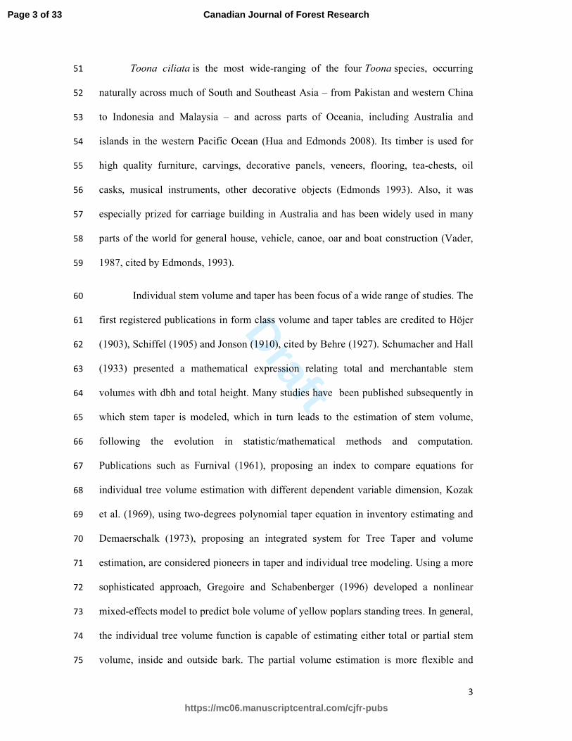
3
Toona ciliata is the most wide-ranging of the four Toona species, occurring 51
naturally across much of South and Southeast Asia – from Pakistan and western China 52
to Indonesia and Malaysia – and across parts of Oceania, including Australia and 53
islands in the western Pacific Ocean (Hua and Edmonds 2008). Its timber is used for 54
high quality furniture, carvings, decorative panels, veneers, flooring, tea-chests, oil 55
casks, musical instruments, other decorative objects (Edmonds 1993). Also, it was 56
especially prized for carriage building in Australia and has been widely used in many 57
parts of the world for general house, vehicle, canoe, oar and boat construction (Vader, 58
1987, cited by Edmonds, 1993). 59
Individual stem volume and taper has been focus of a wide range of studies. The 60
first registered publications in form class volume and taper tables are credited to Höjer 61
(1903), Schiffel (1905) and Jonson (1910), cited by Behre (1927). Schumacher and Hall 62
(1933) presented a mathematical expression relating total and merchantable stem 63
volumes with dbh and total height. Many studies have been published subsequently in 64
which stem taper is modeled, which in turn leads to the estimation of stem volume, 65
following the evolution in statistic/mathematical methods and computation. 66
Publications such as Furnival (1961), proposing an index to compare equations for 67
individual tree volume estimation with different dependent variable dimension, Kozak 68
et al. (1969), using two-degrees polynomial taper equation in inventory estimating and 69
Demaerschalk (1973), proposing an integrated system for Tree Taper and volume 70
estimation, are considered pioneers in taper and individual tree modeling. Using a more 71
sophisticated approach, Gregoire and Schabenberger (1996) developed a nonlinear 72
mixed-effects model to predict bole volume of yellow poplars standing trees. In general, 73
the individual tree volume function is capable of estimating either total or partial stem 74
volume, inside and outside bark. The partial volume estimation is more flexible and 75
Page 3 of 33
https://mc06.manuscriptcentral.com/cjfr-pubs
Canadian Journal of Forest Research

Draft
4
allows multiproduct estimations, such as saw wood, pulp wood, and fuel. The 76
multiproduct estimations are performed by fitting a taper function and, using solid of 77
revolution techniques, the taper function is integrated within a height interval to obtain 78
the partial stem volume. In situations where the average wood density is available for 79
the interval the interval’s mass could be estimated unbiasedly. Furthermore, the 80
availability of a mathematical relationship between mass and carbon also will generate 81
model-unbiased carbon estimation. 82
By definition, the stand timber mass depends on the stem volume and density. 83
The stem wood density is the single most important wood property because its strong 84
relationship to both yield and quality as well as its large variance and heritability 85
(Zobel, 1963). Within the tree, wood density varies from base to top and from pith to 86
bark. Wood density varies because of changes in vessel size and frequency, fiber 87
dimensions (wall thickness and diameter), the percentage of parenchyma (e.g. ray) and 88
wood chemistry (Downes et al. 1997). Luxford & Markwardt (1932), studying the 89
strength and related properties of redwood, found that the specific gravity in redwood 90
stems varied laterally and vertically, and greater values were related to greater crushing 91
strength, side hardness and modulus of rupture. 92
The wood density variation vertically has motivated of study for many other 93
researchers . Zobel and van Buijtenen (1989) cited Chidester et al. (1938) as the pioneer 94
publication in wood density variation. In the study carried out in Eucalyptus regnans in 95
New Zealand, Frederick at al. (1982) found a decline in wood density from the tree base 96
to 1.4 m, with the lowest values occurring at 1.4 m, and higher than that the wood 97
density increases. 98
Also, from pith to bark density variation has been investigated in many research 99
studies. Heitz et al. (2013), collecting wood samples from two neotropical rain forests, 100
Page 4 of 33
https://mc06.manuscriptcentral.com/cjfr-pubs
Canadian Journal of Forest Research
Draft
5
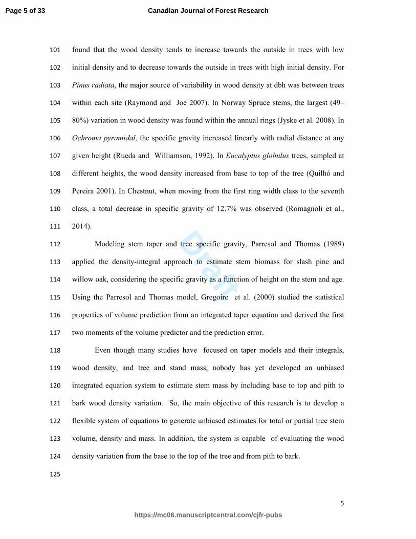
found that the wood density tends to increase towards the outside in trees with low 101
initial density and to decrease towards the outside in trees with high initial density. For 102
Pinus radiata, the major source of variability in wood density at dbh was between trees 103
within each site (Raymond and Joe 2007). In Norway Spruce stems, the largest (49–104
80%) variation in wood density was found within the annual rings (Jyske et al. 2008). In 105
Ochroma pyramidal, the specific gravity increased linearly with radial distance at any 106
given height (Rueda and Williamson, 1992). In Eucalyptus globulus trees, sampled at 107
different heights, the wood density increased from base to top of the tree (Quilhó and 108
Pereira 2001). In Chestnut, when moving from the first ring width class to the seventh 109
class, a total decrease in specific gravity of 12.7% was observed (Romagnoli et al., 110
2014). 111
Modeling stem taper and tree specific gravity, Parresol and Thomas (1989) 112
applied the density-integral approach to estimate stem biomass for slash pine and 113
willow oak, considering the specific gravity as a function of height on the stem and age. 114
Using the Parresol and Thomas model, Gregoire et al. (2000) studied the statistical 115
properties of volume prediction from an integrated taper equation and derived the first 116
two moments of the volume predictor and the prediction error. 117
Even though many studies have focused on taper models and their integrals, 118
wood density, and tree and stand mass, nobody has yet developed an unbiased 119
integrated equation system to estimate stem mass by including base to top and pith to 120
bark wood density variation. So, the main objective of this research is to develop a 121
flexible system of equations to generate unbiased estimates for total or partial tree stem 122
volume, density and mass. In addition, the system is capable of evaluating the wood 123
density variation from the base to the top of the tree and from pith to bark. 124
125
Page 5 of 33
https://mc06.manuscriptcentral.com/cjfr-pubs
Canadian Journal of Forest Research

Draft
6
126
Materials and methods 127
128
Study area and trees sampled 129
The study area is located in the Campo Belo County, Minas Gerais state, Brazil. 130
The Köppen climate classification is Cwa, temperate humid, with dry winter and rainy 131
summer (Köppen, 1900). The warmest month exceeds 22 ° C, with altitude ranging 132
from 790 m to 1146 m and average rainfall of 1250 mm (INMET, 2016). A progeny test 133
was established on February 6, 2008, containing 78 progenies of half-brothers, which 134
were formed from seeds collected in open pollinated arrays in Queensland and New 135
South Wales, Australia. In order to test the progeny performance, a complete block 136
experimental design was installed with 3 replications and 16 trees per sampling unit, 137
and the tree spacing of 3 x 3 m. 138
Selection of trees 139
Two progenies, from Queensland, with better performance were selected and a 140
group of 72 trees were felled (34 trees for the first progeny and 38 for the second 141
progeny), with a mean age of 4.7 years old, based on the normality shape of the 142
diameter (dbh) distribution, i.e 68% of the trees between -1 and 1 standard deviation 143
around of the mean, 95% between -2 and 2 standard deviations and 99% between -3 and 144
3 standard deviations. Using a systematic subsample design, the upper stem diameters, 145
inside and outside bark, were measured at the following heights: 0.15 m (base), 0.7 m, 146
1.3 m (dbh), 30%, 50%, 70% and 85% of the total height. This data were used to fit the 147
taper function. Also, based on the diameter distribution of the felled trees, 6, of the 72 148
trees, were selected for measurement by X-ray densitometry, which generated the 149
Page 6 of 33
https://mc06.manuscriptcentral.com/cjfr-pubs
Canadian Journal of Forest Research

Draft
7
apparent wood density data base. The small size of the subsample of tree was offset by 150
the extensive series of measurement that were taken with each stem. approximately 151
10,000. This was a laborious and expensive process. . The 6 trees were felled and the 152
total height (ht) was measured, using a tape, and samples of 4 cm-disks were taken from 153
the same position as the upper stem diameter measurements, generating a total of 7 154
disks for each tree. Each disk was identified by block, progeny, and tree number. The 155
disks were placed in a fresh air site for drying and subsequently cut and analyzed. 156
Wood density measurements 157
The wood samples were extracted from the sample disks, and density was 158
assessed from pith to bark; each sample was 4 cm wide, 1.6 mm thick, across the radius 159
of the disk. The samples were stored in acclimatized chamber (20 °C, 60% RH) until 160
reaching the moisture content of 12%. The samples were placed on Tree Ring Scanner 161
equipment (QTRS-01X, Quintek Measurement Systems). Knowing moisture content is 162
important since the water present in the chemical components is critical to determining 163
the wood density (QMS, 1999). Since the sample humidity was kept at 12%, the wood 164
density measurements are called Apparent Wood Density (AWD). The equipment 165
scanned the samples and recorded the wood density values at intervals of 0.004 cm 166
apart, from pith to bark. 167
168
Geostatistical Analysis 169
Kriging was used to visualize density variation in a radial and longitudinal 170
approach. This technique, proposed by Krig (1951) and formalized by Matheron (1962), 171
consists in estimating the value z(k) among observations in different spatial locations. 172
Page 7 of 33
https://mc06.manuscriptcentral.com/cjfr-pubs
Canadian Journal of Forest Research

Draft
8
The observations that are close are more correlated than those are far away, quantified 173
as spatial autocorrelation. In a general geostatistic approach, the following variables are 174
defined: u=vector of spatial coordinates (in our case are the stem positions where the 175
apparent density values were observed); z(u)=apparent density values observed at u 176
position; k = position to be estimated z(k) value; h=lag, or spatial distance, between k 177
and each u spatial location; z(u+h)=lagged version of apparent density; N(h)=number 178
of points separated by lag h. z(u) is called tail variable and z(u+h) is referred to as the 179
head. After the lag vector is determined, the covariance, correlation and semivariance 180
are estimated and the parameters range, sill and nugget are calculated from 181
semivariance function. Based on semivariance parameters, a semivariance model is 182
chosen and the covariance vector values are estimated using the semivariance 183
parameters and the model. A covariance matrix N x N is also estimated based on the 184
distance between each u and k position. The weight for each N position is estimated by 185
the product of the inverse of covariance matrix and the covariance vector. The residual 186
for the k position is estimated by the product of weight vector and the difference of z() 187
value for each N position and the general mean value. The estimated value for the k 188
position z(k) is the sum of residual value and the general mean value. Performing this 189
analysis varying the k value, the apparent density will be interpolated for the whole 190
stem and a consistent representation and its variation will be generated. 191
192
System of Equations 193
Model Development 194
We present a system of equations which integrate stem volume, wood density 195
and stem mass estimation. Assuming that the wood specific gravity is the ratio between 196
Page 8 of 33
https://mc06.manuscriptcentral.com/cjfr-pubs
Canadian Journal of Forest Research
Draft
9
the wood density and water density, and the water density is equal to 1 (g.cm-3 or Mg.m-197
3), we will use the expression (1) to estimate wood mass, in Mg. In this specific case, 198
following the x-ray methodology, the mass will be estimated with 12% of moisture 199
content, the volume will be green and the density will be treated as Apparent Wood 200
Density (AWD). 201
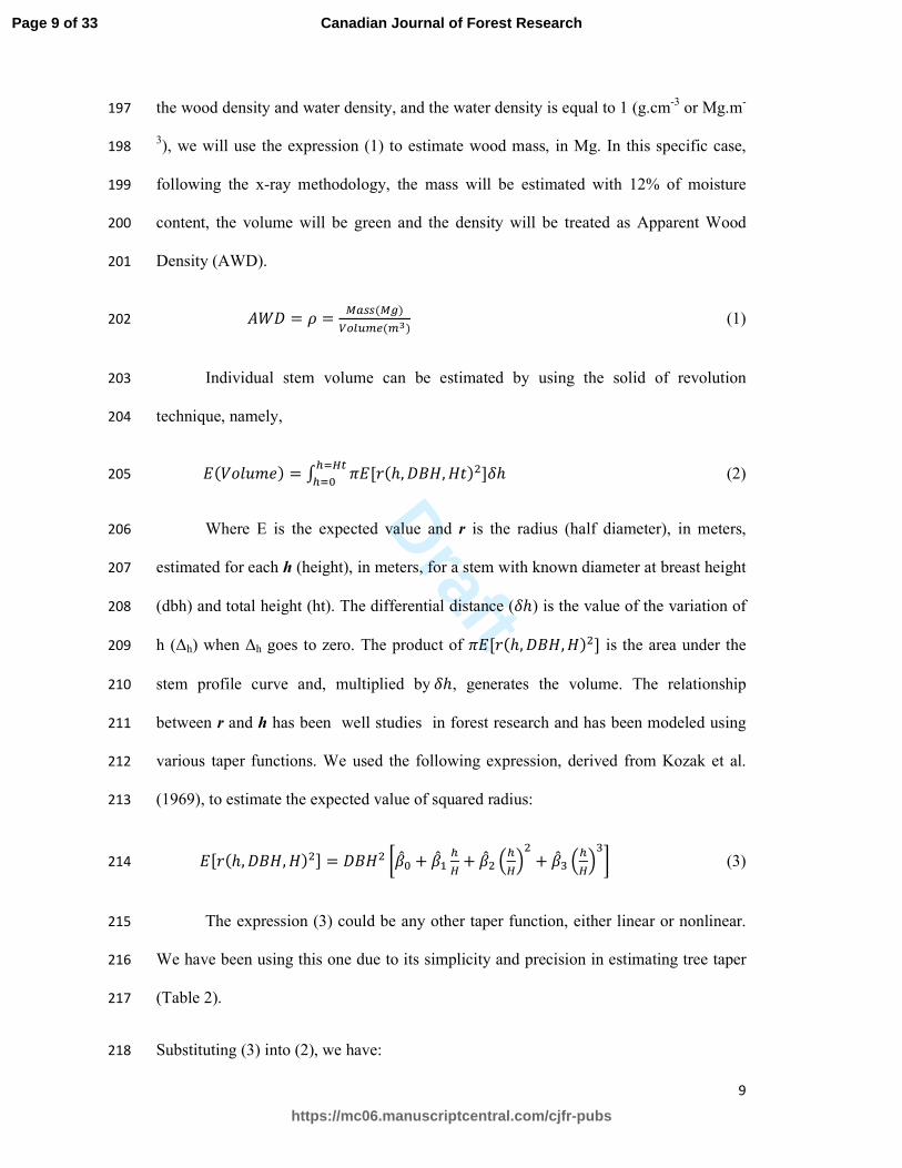
��� = � = ����(�)� ����(��) (1) 202
Individual stem volume can be estimated by using the solid of revolution 203
technique, namely, 204
�(������) = � ��[�(ℎ, � !,!")#]%ℎ&'()&'* (2) 205
Where E is the expected value and r is the radius (half diameter), in meters, 206
estimated for each h (height), in meters, for a stem with known diameter at breast height 207
(dbh) and total height (ht). The differential distance (%ℎ) is the value of the variation of 208
h (∆h) when ∆h goes to zero. The product of ��[�(ℎ, � !,!)#] is the area under the 209
stem profile curve and, multiplied by%ℎ, generates the volume. The relationship 210
between r and h has been well studies in forest research and has been modeled using 211
various taper functions. We used the following expression, derived from Kozak et al. 212
(1969), to estimate the expected value of squared radius: 213
�[�(ℎ, � !,!)#] = � !# ,-.* + -.0 &( + -.# 1&(2# + -.3 1&(234 (3) 214
The expression (3) could be any other taper function, either linear or nonlinear. 215
We have been using this one due to its simplicity and precision in estimating tree taper 216
(Table 2). 217
Substituting (3) into (2), we have: 218
Page 9 of 33
https://mc06.manuscriptcentral.com/cjfr-pubs
Canadian Journal of Forest Research

Draft
10
�(������) = � � 5� !# ,-.* + -.0 &( + -.# 1&(2# + -.3 1&(2346 %ℎ&'()&'* (4) 219
When the stem wood density value is known and there is no variation from base 220
to top and from the pith to the bark of the tree, the following relation would be 221
appropriate in order to estimate stem mass. 222
�(7899) = � ��[�(ℎ, � !,!")#]%ℎ&'&)&'* ∗ � (5) 223
If the density varies from base to top of the tree, we could use a function 224
E[�(ℎ)] instead of�, where the expression �[�(ℎ)] explains the expected density as a 225
function of height. 226
�(7899) = � ��[�(ℎ, � !,!")#]%ℎ&'&)&'* ∗ �[�(ℎ)] (6) 227
If the density varies from both the base to the top of the tree and pith to bark, the 228
variation would be explained by height and radius �[�(ℎ, �)] and the mass estimation 229
expression would be: 230
E(Mass)=∑ > � πE[�(ℎ, � !,!")#]δhh=ht@
h=0*E[ρ(h,r)]
-� πE A(�(ℎ, � !,!")-∆C)2D δh
h=ht@h=0
* EEρFh,r-∆CGHI0 by ∆Jr=rmax (7) 231
The expression (7) is a combination of continuous and discrete sum. The first 232
integral of the difference inside the braces estimates the stem mass with height varying 233
from base to the top of the tree and in radial position r. The second integral estimate the 234
stem mass, but with radius equal r-∆r, where ∆r is the incremental shell thickness. The 235
difference between the two integrals generates the shell mass, with expected density 236
E[ρ(h,r)]. The sum of the differences results in stem total mass. If we use the lim ∆r=0, 237
then the expression (7) would be: 238
Page 10 of 33
https://mc06.manuscriptcentral.com/cjfr-pubs
Canadian Journal of Forest Research
Draft
11
E(Mass)=� > � πE[�(ℎ, � !,!")2]δhh=ht@
h=0*E[ρ(h,r)]δr
-� πE[(�(ℎ, � !,!")-δr)2]δh
h=ht@h=0
*EEρFh,r-δrGHδrI0
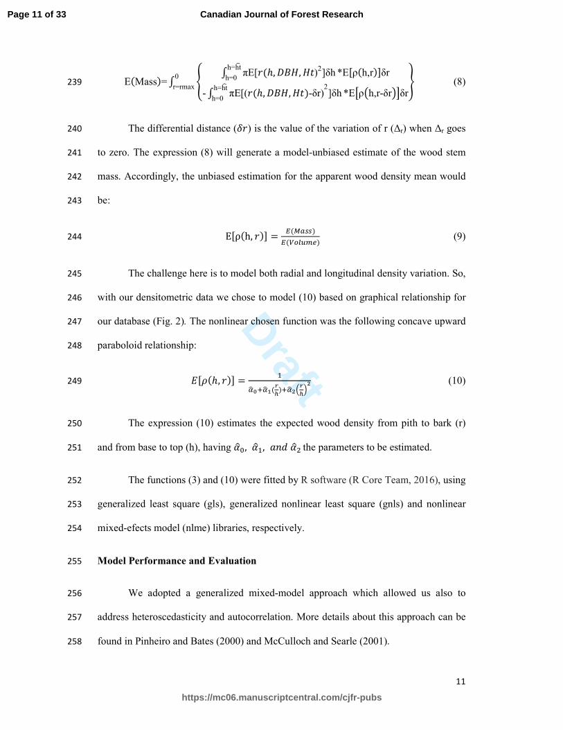
r=rmax (8) 239
The differential distance (%�) is the value of the variation of r (∆r) when ∆r goes 240
to zero. The expression (8) will generate a model-unbiased estimate of the wood stem 241
mass. Accordingly, the unbiased estimation for the apparent wood density mean would 242
be: 243
E[ρ(h, �)] = N(����)N(� ����) (9) 244
The challenge here is to model both radial and longitudinal density variation. So, 245
with our densitometric data we chose to model (10) based on graphical relationship for 246
our database (Fig. 2). The nonlinear chosen function was the following concave upward 247
paraboloid relationship: 248
�[�(ℎ, �)] = 0OPQROPS(JT)ROPU1JT2U (10) 249
The expression (10) estimates the expected wood density from pith to bark (r) 250
and from base to top (h), having VW*, VW0, 8XYVW#the parameters to be estimated. 251
The functions (3) and (10) were fitted by R software (R Core Team, 2016), using 252
generalized least square (gls), generalized nonlinear least square (gnls) and nonlinear 253
mixed-efects model (nlme) libraries, respectively. 254
Model Performance and Evaluation 255
We adopted a generalized mixed-model approach which allowed us also to 256
address heteroscedasticity and autocorrelation. More details about this approach can be 257
found in Pinheiro and Bates (2000) and McCulloch and Searle (2001). 258
Page 11 of 33
https://mc06.manuscriptcentral.com/cjfr-pubs
Canadian Journal of Forest Research

Draft
12
The evaluation criteria used were Root Mean Square Error (RMSE) and 259
Coefficient of Determination (R2), presented in (11) and (12). After improving the 260
models by generalized mixed approach the Akaike Information Criterion (AIC) 261
(Sakamoto et al. 1986) and Likelihood Ratio Test (LRT) were used to evaluate the 262
model improvements. The expressions for these are shown in (13) and (14). 263
264
Z7[� = \∑ (]^_]W^)U`̂aS(b_c) (11) 265
Z# = ∑ (]dP _]e)U`̂aS∑ (]^_]e)U`̂aS ∗ 100 (12) 266
�hi = −2�(lm/o) + 2Xc�C (13) 267
pZq = 2ln(ptu#ptu0) In these formulas yi is the observed value for the ith observation, oWv is the 268
estimated value, n is the number of total observation, p is the number of parameters in 269
the model, oe is the mean of the observed values, �(lm/o) is the natural logarithm of the 270
profiled likelihood for the vector parameter lm as a function of the observed values for y, 271
Lik1 is the likelihood value for the restricted model and Lik2 is the likelihood value for 272
the general model. Under the null hypothesis that the restricted model is more adequate, 273
the distribution for LRT is χ2 with k2-k1 degrees of freedom. 274
275
Results 276
Fitting taper and apparent density functions 277
Page 12 of 33
https://mc06.manuscriptcentral.com/cjfr-pubs
Canadian Journal of Forest Research

Draft
13
Taper (3) and density (10) functions were fitted in order to model volume and 278
mass. Table 1 summarizes the statistics for the trees selected for taper and apparent 279
density measurements. The source of variation among plants for both taper and apparent 280
density databases are from genetic and environmental factors. Environmental factors 281
such as competition index, fertilization, pest and disease and seedling quality are 282
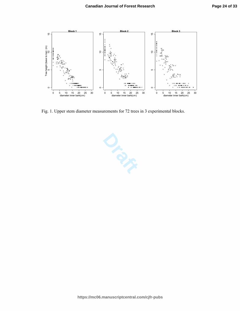
determinant source that explain the variation among the sampled trees. The upper stem 283
diameter measurements for the 72 sample trees, within three blocks, are displayed in 284
Fig. 1. As is apparent, the diameter at the base of trees varies from 15 to about 30 cm 285
and stem height varies from 6 to 15 meters. 286
Fig. 1. 287
The apparent density relationships with the ratio between radius, from pith to 288
bark, and height, from base to top, also including a loess smooth pattern, are displayed 289
in Fig. 2. The first remark is an observed decrease trend follows by an increase of the 290
apparent density when the ratio between radius and height increases. 291
Fig.2. 292
A better representation, including both radial and longitudinal density variation 293
for each tree, can be observed in Fig. 3, in which kriging geostatistical techniques were 294
applied to model the bidirectional variation. Also called Gaussian process regression, 295
with this technique it is possible to interpolate, or estimate, the density values in the 296
stem positions where the wood samples were not collected. As shown, the density, in 297
general, increases from pith to bark and from base to top.. 298
Parameter estimates and model statistics for taper function (3) and apparent 299
density function (10) are shown in Table 2. In both functions, the p-values for all 300
parameters were significant, considering α=0.05 (or 5%), ratifying the capacity of these 301
Page 13 of 33
https://mc06.manuscriptcentral.com/cjfr-pubs
Canadian Journal of Forest Research

Draft
14
models to explain the observed variation in stem volume and density within the stem. 302
When modeling stem taper, heteroscedasticity and autocorrelation was also modeled, 303
using the gls function from nlme R package (Pinheiro and Bates 2000). The Akaike 304
Information Criterion (AIC) decreases from -2188 to -3030, having a likelihood ratio 305
test value of 846 and p-value <0.0001, meaning that the heteroscedastic and 306
autocorrelated model had better performance than a reduced model assuming 307
homoscedastic and independent observations. 308
Fig. 3 309
Fig. 4 depicts, for taper equation, the improvement in the residual distribution 310
after modeling heteroscedasticity and autocorrelation. For apparent density function, 311
due to the height variation between trees and within each tree, heteroscedasticity and 312
autocorrelation were also modeled by considering the model as a two-level mixed-313
effect: tree level and height position level within tree level (Pinheiro and Bates 2000). 314
The AIC values before and after modeling were, respectively, -1701 and -2513, 315
generating a likelihood ratio test value of 828 and p-value <0.0001. Fig. 5 shows a 316
centered in zero and constant residual distribution within and among trees after 317
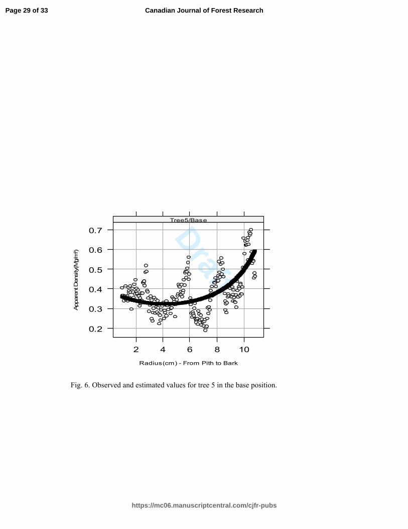
heteroscedasticity and autocorrelation modeling. A better resolution of the curvilinear 318
U-shape observed and estimated apparent density for tree 5 in the base position is 319
shown in Fig. 6. 320
321
Fig. 4. 322
323
Fig. 5. 324
325
Page 14 of 33
https://mc06.manuscriptcentral.com/cjfr-pubs
Canadian Journal of Forest Research

Draft
15
Fig. 6. 326
Estimating mass 327
Density varying from base to top 328
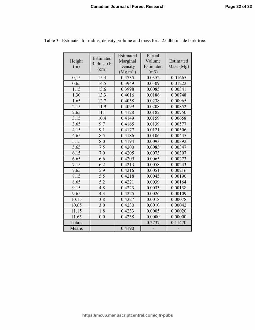
In order to exemplify the stem biomass assessment, the functions (3) and (10), 329
after fitting, were used to estimate the partial volume and mass of a sample tree, picked 330
among 72 harvested trees, with dbh inside bark of 25 cm and a total height of 11.65 m 331
(Table 3). The radius values, for each height position, were estimated by the taper 332
function. The density estimates were called marginal because its estimate used as 333
independent variables the height position and the external values of inside bark radius 334
for each height position. The apparent wood density, Mg.m-3, decreases from 0.4735, at 335
height of 0.15 m, to 0.3949, at height of 0.65 m. After that, the density increases until 336
the top of the tree, reaching 0.4238. The average density, stem volume and stem mass 337
were, respectively, 0.4190 Mg.m-3, 0.2734 m3 and 0.1147 Mg. A common practice is to 338
multiply the dbh density value (0.4016 Mg.m-3) with stem volume (0.2737 m3) in order 339
to estimate the stem mass. If we do so, the estimated mass is 0.1099 Mg and, compared 340
to 0.1147 Mg, which demonstrates a bias of 4.18%. 341
342
Density varying from base to top and from pith to bark. 343
Also for a 25 cm dbh and 11.65 m height tree, the fitted functions (3) and (10) 344
were substituted into the function (7), with ∆=2.5 cm, in order to generate a more 345
precise mass estimation. This procedure subdivided the tree into 4 shells and a core 346
stem. The shell thickness and the core stem radius at breast height were 2.5 cm, 347
increasing to the tree base and decreasing to the tree top, following the sigmoidal-shape 348
taper function estimates. The results are displayed in Table 4. The outer shell, from 20 349
Page 15 of 33
https://mc06.manuscriptcentral.com/cjfr-pubs
Canadian Journal of Forest Research

Draft
16
to 25 cm of dbh, represents roughly 40% of the total volume and mass. This percentage 350
decreases about 10% for each inner shell and for core stem. The estimated stem volume 351
was 0.2737 m3, which is the same value in Table 3, showing consistent estimates for 352
each shell and for stem core. The estimated stem mass was 0.1131 Mg. This value was 353
estimated by the sum of the mass for each shell and core stem. That is, base to top and 354
pith to bark density values were multiplied by each volume value to generate the stem 355
mass. Compared to the mass value estimated by taking the outer density from base to 356
top, 0.1147 Mg (Table 3), the bias is 1.4%. This value increases with the density 357
variation in both from base to top and from pith to bark. The mean density, estimated 358
by expression (9), was 0.4132 Mg.m-3. In the sample tree, this value is located at heights 359
around 2.5m, 2.0m, 1.5m, 1.0m, and 0.5m for the first, second, third, fourth shell and 360
core stem, respectively. The stem mass also was estimated using the double integral, 361
with limit of ∆r goes to 0, following expression (8). The estimated value was 0.1128 362
Mg, which is very close to the value estimated by summing, with ∆r=2.5 cm (0.1131 363
Mg), and the bias was 0.26%. Taking in account the stem volume, 0.2737 cubic meters, 364
the mean density was 0.4121 Mg.m-3, which is a slightly smaller than the estimated 365
value in expression (7). 366
367
Discussion 368
Taper and density functions 369
The relatively small variation in dbh and height in our sample trees is due to the 370
young plantation age, about 4.7 years old. In apparent density database, the minimum 371
threshold dbh was fixed at 15 cm, since logs will be our final gross product. The greater 372
vertical and horizontal variation of the observed apparent density values are due to 373
Page 16 of 33
https://mc06.manuscriptcentral.com/cjfr-pubs
Canadian Journal of Forest Research
Draft
17
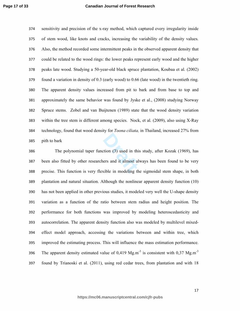
sensitivity and precision of the x-ray method, which captured every irregularity inside 374
of stem wood, like knots and cracks, increasing the variability of the density values. 375
Also, the method recorded some intermittent peaks in the observed apparent density that 376
could be related to the wood rings: the lower peaks represent early wood and the higher 377
peaks late wood. Studying a 50-year-old black spruce plantation, Koubaa et al. (2002) 378
found a variation in density of 0.3 (early wood) to 0.66 (late wood) in the twentieth ring. 379
The apparent density values increased from pit to bark and from base to top and 380
approximately the same behavior was found by Jyske et al., (2008) studying Norway 381
Spruce stems. Zobel and van Buijtenen (1989) state that the wood density variation 382
within the tree stem is different among species. Nock, et al. (2009), also using X-Ray 383
technology, found that wood density for Toona ciliata, in Thailand, increased 27% from 384
pith to bark 385
The polynomial taper function (3) used in this study, after Kozak (1969), has 386
been also fitted by other researchers and it almost always has been found to be very 387
precise. This function is very flexible in modeling the sigmoidal stem shape, in both 388
plantation and natural situation. Although the nonlinear apparent density function (10) 389
has not been applied in other previous studies, it modeled very well the U-shape density 390
variation as a function of the ratio between stem radius and height position. The 391
performance for both functions was improved by modeling heteroscedasticity and 392
autocorrelation. The apparent density function also was modeled by multilevel mixed-393
effect model approach, accessing the variations between and within tree, which 394
improved the estimating process. This will influence the mass estimation performance. 395
The apparent density estimated value of 0,419 Mg.m-3 is consistent with 0,37 Mg.m-3 396
found by Trianoski et al. (2011), using red cedar trees, from plantation and with 18 397
Page 17 of 33
https://mc06.manuscriptcentral.com/cjfr-pubs
Canadian Journal of Forest Research

Draft
18
years old. This value would be close to 0.4 Mg.m-3 in apparent density, instead specific 398
gravity, due to 12% of humidity. 399
400
Mass estimation 401
When the stem mass was estimated taking in account the density variation from 402
base to the top of the tree, the average estimated density was found at approximately 5.0 403
meters of height, about 43% of the total height. Pérez-Cruzado and Rodríguez-Soalleiro 404
(2009), studying Eucalyptus nittens, found that the average basic density occurs at a 405
relative height of 30–35% along the stem. Compared to the mass estimated by using the 406
apparent density value at dbh, the bias generated was 4,2%. This is a significant value 407
compared to, for example, forest sample error, which could be, in some situation, 408
smaller than 5%. Indeed, the bias will be directly related to the variation of the base-to-409
top apparent density and when the apparent density mean value is located far from dbh 410
position. Greater variation, in this case, implies greater bias. 411
When stem mass was estimated considering the density variations from base 412
to top and form pith to bark, considering the radius variation as a discrete approach 413
(∆=2.5 cm), the bias was 1,4%, compared to the mass estimated accounted just with 414
base to top density variation. Again, the bias would be correlated to the stem density 415
variation, as opposed to assuming constant density presumably from its value at breast 416
height. 417
418
Conclusions 419
In general, the apparent density values increased from base to top and from the 420
pith to the bark for each tree, in a nonlinear U-shape trend. The proposed system of 421
Page 18 of 33
https://mc06.manuscriptcentral.com/cjfr-pubs
Canadian Journal of Forest Research

Draft
19
equations fitted very well the tree taper and the tree density variation. Compared to the 422
traditional method, which the density values at dbh are used to estimate the stem mass, 423
the bias estimation was reduced by accessing the density variation from the base to the 424
top of the tree. Also, the estimation of mass was improved by modeling the density 425
variation from both base to top and pith to bark. The model performance was improved 426
by using the generalized linear and nonlinear mixed-effects approach. The system can 427
be used to estimate stem volume, density and mass for every red cedar tree a least 5 428
years old, at the study location, having dbh and total height measurements. As a future 429
study suggestion, using older tree and different sites database would generate a more 430
practical application system for this and other plant species. 431
432
Acknowledgements 433
The authors thank to CNPq and Fapemig, the Brazilian and Minas Gerais State research 434
sponsors, respectively. 435
436
References 437
Behre, C.E. 1927. Form-class taper curves and volume tables and their application. 438
Journal of Agricultural Research 35(8): 673-744. 439
Chidester G.H., McGovern I.N., McNaughton G.C. 1938. Comparison of sulfite pulps 440
from fast grown loblolly, shortleaf, longleaf and slash pines. Paper Tr J 107, 441
Tappi Sec: 32-35 442
Clutter, J.L. 1980. Development of taper functions from variable-top merchantable 443
volume equations. Forest Science 26(1):117-120. 444
Page 19 of 33
https://mc06.manuscriptcentral.com/cjfr-pubs
Canadian Journal of Forest Research
Draft
20
Demaerschalk, J.P. 1973. Integrated systems for the estimation of tree taper and 445
volume. Canadian Journal of Forest Research. 3(90):90-94. 446
Downes G.M., Hudson I.L., Raymond C.A., Dean G.H., Michell A.J., Schimleck L.R., 447
Evans R., Muneri A. 1997. Sampling plantation eucalypts for wood and fibre 448
properties, CSIRO Publishing, Melbourne, 1997. 449
Edmonds, J. 1993. The potential value of Toona species (Meliaceae) as multipurpose 450
and plantation trees in Southeast Asia. The Commonwealth 451
ForestryReview, 72(3), 181-186. Retrieved from 452
http://www.jstor.org/stable/42616713 453
Frederick, D. J., Madgwick H. A. I., Oliver, G. R. 1982. Wood basic density and 454
moisture content of young Eucalyptus regnans grown in New Zealand. New 455
Zealand Journal of Forestry Science 12(3): 49. 456
Furnival, George M. 1961. An index for comparing equations used in constructing 457
volume tables. Forest Science. 7: 337-341. 458
Gregoire, T.G. and O. Schabenberger. 1996. A Non-linear mixed-effects model to 459
predict cumulative bole volume of standing trees. Journal of Applied Statistics 460
23(2&3):257-271. 461
Gregoire, T.G. ,Schabenberger, O., Kong F. 2000. Prediction from an Integrated 462
Regression Equation: A Forestry Application. Biometrics 56. 414-419. 463
Heitz, P., Valencia, R., Wright, S. J. 2013. Strong radial variation in wood density 464
follows a uniform pattern in two neotropical rain forests. Functional Ecology. 465
Höjer, A. G. 1903. Bihang till fr. loven: Om vӓra barrskogar. Stockholm. 466
Hua P., Edmonds J.M. 2008. Toona (Endlicher) M. Roemer, Fam. Nat. Syn. Monogr. 1: 467
131. 1846. In: Flora of China, vol. 11: Oxalidaceae through Aceraceae. St Louis, 468
MO, USA: Missouri Botanical Garden, 112-115. 469
Page 20 of 33
https://mc06.manuscriptcentral.com/cjfr-pubs
Canadian Journal of Forest Research
Draft
21
INMET. 2016. Climatological station net. Brazilian Meteorological Institute. (accessed 470
in 07/05/2016 - http://www.inmet.gov.br). 471
Jonson, T.1910. Taxatoriska undersökningar om skogsträdens form. I. Granens 472
Stamform. Skogsvardsför. Tidskr. 8 (11): 285-328, illus. 473
Jyske, T., Mäkinen, H., Saranpää, P. 2008. Wood density within norway spruce stems. 474
Silva Fennica 42(3) 475
Köppen, W. 1900. Versuch einer klassifikation der klimate, vorzugsweise nach ihren 476
Beziehungen zur Pflanzenwelt. Geographische Zeitschrift 6, 657–679. 477
Koubaa A., Zhangb, S.Y.T. and Maknic S. 2002. Defining the transition from 478
earlywood to latewood in black spruce based on intra-ring wood density profiles 479
from X-ray densitometry. Ann. For. Sci. 59 511–518. 480
Kozak, A., D.D. Munro, and J.H.G. Smith. 1969. Taper functions and their application 481
in forest inventory. The Forestry Chronicle 45:278-283. 482
Krige, Danie G. 1951. A statistical approach to some basic mine valuation problems on 483
the Witwatersrand. J. of the Chem., Metal. and Mining Soc. of South 484
Africa. 52 (6): 119–139. 485
Luxford, R. F., Markwardt, L.J. 1932. The strength and related properties of redwood. 486
USDA Technical Bulletin No. 305. Washington, D.C. 487
Matheron, G. 1962. Traité de géostatistique appliquée. Editions Technip. 488
489
McCulloch, C.E. and Searle, S.R. 2001. Generalized, Linear, and Mixed Models, 490
Wiley, New York. 491
Nock, C.A., Geihofer, D., Grabner M., Baker,P.J., Bunyavejchewin S. and Hietz, P. 492
2009. Wood density and its radial variation in six canopy tree species differing in 493
shade-tolerance in western Thailand. Annals of Botany 118:1-10. 494
Page 21 of 33
https://mc06.manuscriptcentral.com/cjfr-pubs
Canadian Journal of Forest Research
Draft
22
Parresol, B.R., and Thomas, C.E. 1989. A density-integral approach to estimating stem 495
biomass. For. Ecol. Manage. 26: 285-297. 496
Pérez-Cruzado C. and Rodríguez-Soalleiro R. 2009. Improvement in accuracy of 497
aboveground biomass estimation in Eucalyptus nitens plantations: Effect of bole 498
sampling intensity and explanatory variables. Forest Ecology and Management. 499
261. 2016-2028. 500
QMS (QUINTEK MEASUREMENT SYSTEMS). 1999. Tree ring analyzer users guide 501
- Model QTRS-01X. Knoxville.72 p. 502
Quilhó, T., Pereira, H. 2001. Within and between tree variation of bark content and 503
wood density of Eucalyptus globulus in commercial plantations. Iawa Journal, 504
Vol. 22 (3), 2001: 255–265. 505
Raymond, C.A. and Joe, B. 2007. Patterns of basic density variation for Pinus 506
radiata grown in south-west slopes region of New South Wales, Australia. New 507
Zealand Journal of Forestry Science 37(1): 81–95. 508
Ribeiro Jr., P.J. & Diggle, P.J. 2001. geoR: A package for geostatistical analysis. R-509
NEWS, Vol 1, No 2, 15-18. ISSN 1609-3631. 510
Romagnoli, M., Cavalli, D., Spina, S. 2014. Chestnut wood quality. BioResources 9(1). 511
R Core Team (2016). R: A language and environment for statistical computing. R 512
Foundation for Statistical Computing, Vienna, Austria. URL https://www.R-513
project.org/. 514
Rueda R., Williamson G. B. 1992. Radial and vertical wood specific gravity 515
in Ochroma pyramidale (Cav. ex Lam.) Urb. (Bombacaceae). Biotropica 24:512–516
518. 517
Sakamoto, Y., Ishiguro, M. and Kitagawa, G. 1986. Akaike Information Criterion 518
Statistics, Reidel, Dordrecht, Holland. 519
Page 22 of 33
https://mc06.manuscriptcentral.com/cjfr-pubs
Canadian Journal of Forest Research

Draft
23
Schiffel, A. 1905. Form und inhalt der lärche. Mitt. Forstl. Versuchsw. Österr., Heft 31, 520
122 p., illus. 521
Schumacher, F.X. 1926. A Method of measuring form quotient of standing trees. 522
Journal of Forestry 24:552-554. 523
Trianoski, R., Iwakiri, S., De Matos, J.L.M. 2011. Potential use of planted fast-growing 524
species for production of particleboard. Journal of Tropical Forest Science, 311-525
317. 526
Vader, J. 1987. Red cedar: the tree of Australia’s history. Reed. NSW. pp. 200. 527
Wiemann, M. C., and Williamson,G.B. 1989a. Radial gradients in the specific gravity 528
of wood in some tropical and temperate trees. Forest Science 35 : 197 – 210 . 529
Zobel, B.J., van Buijtenen, J. P.1989 . Wood variation: Its causes and control. Spring 530
Verlag, New York. 531
Page 23 of 33
https://mc06.manuscriptcentral.com/cjfr-pubs
Canadian Journal of Forest Research
Draft
Fig. 1. Upper stem diameter measurements for 72 trees in 3 experimental blocks.
o
o
o
o
o
o
o
o
o
o
o
o
o
o
o
o
o
o
o
o
o
o
o
o
o
o
o
o
o
o
o
o
o
o
o
o
o
o
o
o
o
o
o
o
o
o
o
o
o
o
o
o
o
o
o
o
o
o
o
o
o
o
o
o
o
o
o
o
o
o
o
o
o
o
o
o
o
o
o
o
o
o
o
o
o
o
o
o
o
o
o
o
o
o
o
o
o
o
o
o
o
o
o
o
oo
o
o
o
o
o
o
o
o
o
o
o
o
oo
o
o
o
o
o
o
o
o
o
o
o
o
o
o
o
o
o
o
o
o
o
o
o
o
o
o
o
o
o
o
o
o
o
o
o
o
o
o
o
o
o
o
o
o
o
o
o
o
o
o
o
o
o
o
o
o
o
o
o
o
o
o
o
o
o
o
o
o
o
o
o
o
o
o
o
o
o
o
o
o
0 5 10 15 20 25 30
05
10
15
diameter inner bark(cm)
Tre
e h
eig
ht (b
ase to top)
(m
)
Block 1
o
o
o
o
o
o
o
o
o
o
o
o
o
o
o
o
o
o
o
o
o
o
o
o
o
o
o
o
o
o
o
o
o
o
o
o
o
o
o
o
o
o
o
o
o
o
o
o
o
o
o
o
o
o
o
o
o
o
o
o
o
o
o
o
o
o
o
o
o
o
o
o
o
o
o
o
o
o
o
o
o
o
o
o
o
o
o
o
o
o
o
o
o
o
o
o
o
o
o
o
o
o
o
o
o
o
o
o
o
o
o
o
o
o
o
o
o
o
o
o
o
o
o
o
o
o
o
o
o
o
o
o
o
o
o
o
o
o
o
o
o
o
o
o
o
o
o
o
o
o
o
o
o
o
o
o
o
o
o
o
o
o
o
o
o
o
o
o
o
o
o
o
o
o
o
o
o
o
o
o
o
o
o
o
o
o
o
o
o
o
o
o
o
o
o
o
o
o
o
o
0 5 10 15 20 25 30
05
10
15
diameter inner bark(cm)
Block 2
o
o
o
o
o
o
o
o
o
o
o
o
o
o
o
o
o
o
o
o
o
o
o
o
o
o
o
o
o
o
o
o
o
o
o
o
o
o
o
o
o
o
o
o
o
o
o
o
o
o
o
o
o
o
o
o
o
o
o
o
o
o
o
o
o
o
o
o
o
o
o
o
o
o
o
o
o
o
o
o
o
o
o
o
o
o
o
o
o
o
o
o
o
o
o
o
o
o
o
o
o
o
o
o
o
o
o
o
o
o
o
o
o
o
o
o
o
o
o
o
o
o
o
o
o
o
o
o
o
o
o
o
o
o
o
o
o
o
o
o
o
o
o
o
o
o
o
o
o
o
o
o
o
o
o
o
o
o
o
o
o
o
o
o
o
o
o
o
o
o
o
o
o
o
o
o
0 5 10 15 20 25 30
05
10
15
diameter inner bark(cm)
Block 3
Page 24 of 33
https://mc06.manuscriptcentral.com/cjfr-pubs
Canadian Journal of Forest Research

Draft
Fig.2. Variation of the apparent density as a function of the ratio between radius and
height for 6 sample trees with a loess smoother line to portray the pattern of the
relationship.
0.3
0.4
0.5
0.6
0.7
0.8
0 20 40 60
Tree 1 Tree 2
0 20 40 60
Tree 3
Tree 4
0 20 40 60
Tree 5
0.3
0.4
0.5
0.6
0.7
0.8Tree 6
Radius(cm)/Height(m)
Appare
nt
Density(M
g/m
3)
Page 25 of 33
https://mc06.manuscriptcentral.com/cjfr-pubs
Canadian Journal of Forest Research

Draft
Figure 3. Kriging of observed apparent density for sample trees
Page 26 of 33
https://mc06.manuscriptcentral.com/cjfr-pubs
Canadian Journal of Forest Research

Draft
Fig. 4. Residual distribution before (A) and after (B) heteroscedasticity and
autocorrelation modeling for taper model.
(A)
Fitted Taper Values (r/dbh)²)
Sta
ndard
ized r
esid
uals
-4
-2
0
2
4
0.0 0.1 0.2 0.3 0.4
Ѫ
ѪѪ
ѪѪ
ѪѪѪ
ѪѪ
Ѫ
Ѫ
Ѫ
ѪѪ
Ѫ
Ѫ
Ѫ
Ѫ
ѪѪ
ѪѪѪ
Ѫ
ѪѪ
ѪѪ
ѪѪ
Ѫ
Ѫ
Ѫ
Ѫ
ѪѪ
ѪѪѪ
ѪѪ
ѪѪ
ѪѪѪѪ
Ѫ
Ѫ
Ѫ
Ѫ
ѪѪѪ
ѪѪѪ
ѪѪ
ѪѪ
Ѫ
ѪѪ
ѪѪѪ
ѪѪѪ
Ѫ
ѪѪѪ
ѪѪ
ѪѪ
ѪѪ
Ѫ
Ѫ
ѪѪѪ
Ѫ
ѪѪ
ѪѪѪѪ
ѪѪ
ѪѪ
ѪѪѪѪ
Ѫ
Ѫ
ѪѪ
Ѫ
Ѫ
ѪѪѪ
Ѫ
ѪѪ
ѪѪѪѪ
Ѫ Ѫ
ѪѪ
Ѫ
ѪѪѪѪ
Ѫ
ѪѪѪ
Ѫ
ѪѪѪ
Ѫ
Ѫ
Ѫ
ѪѪѪѪ
Ѫ Ѫ
Ѫ
Ѫ
Ѫ
ѪѪ
ѪѪ
Ѫ
ѪѪ
ѪѪ
ѪѪ
Ѫ
Ѫ
ѪѪ
ѪѪѪѪ
Ѫ
Ѫ
ѪѪ
ѪѪ
ѪѪѪ
ѪѪ
Ѫ
ѪѪ
ѪѪѪ
Ѫ
ѪѪ
ѪѪ
ѪѪ
Ѫ
Ѫ
ѪѪѪѪѪ
Ѫ
Ѫ
ѪѪ
ѪѪ
ѪѪ
ѪѪ
Ѫ
Ѫ
ѪѪ
ѪѪѪ
Ѫ
Ѫ
ѪѪ
Ѫ
ѪѪ
ѪѪ
ѪѪ
ѪѪ
ѪѪ
ѪѪ
Ѫ
ѪѪ
ѪѪ
Ѫ ѪѪѪ
ѪѪ
Ѫ
ѪѪ
Ѫ
Ѫ
ѪѪ
ѪѪѪѪ
Ѫ
ѪѪ
ѪѪ
ѪѪ
Ѫ
Ѫ
Ѫ
Ѫ
ѪѪ
ѪѪ
Ѫ
Ѫ
ѪѪ
Ѫ
ѪѪѪ
Ѫ
Ѫ
ѪѪ
ѪѪ
ѪѪѪ
Ѫ
ѪѪ
ѪѪ
ѪѪ
Ѫ
Ѫ
ѪѪ
ѪѪ
ѪѪ
Ѫ
ѪѪѪ
ѪѪѪѪ
Ѫ
ѪѪѪ
ѪѪ
ѪѪѪ
Ѫ
ѪѪ
ѪѪѪ
ѪѪ
Ѫ
ѪѪ
ѪѪ
ѪѪ
Ѫ
Ѫ
Ѫ
ѪѪ
Ѫ
ѪѪ
Ѫ
ѪѪ
ѪѪѪ
ѪѪ Ѫ
ѪѪ
ѪѪ
ѪѪѪ
Ѫ
ѪѪѪ
ѪѪѪ
Ѫ
Ѫ
ѪѪ
ѪѪѪ
ѪѪ
ѪѪ
Ѫ
ѪѪ
ѪѪѪ
Ѫ
ѪѪ
ѪѪѪѪѪ
Ѫ
Ѫ
ѪѪѪѪ
Ѫ
ѪѪ
ѪѪ
ѪѪ
ѪѪ
Ѫ ѪѪ
Ѫ
ѪѪ
ѪѪѪ
ѪѪ
Ѫ
ѪѪѪѪ
Ѫ
Ѫ
ѪѪѪѪ
ѪѪ
Ѫ
Ѫ
Ѫ
ѪѪ
Ѫ
ѪѪ
Ѫ
Ѫ
ѪѪ
ѪѪ
Ѫ
ѪѪ
Ѫ
ѪѪ
Ѫ
ѪѪѪѪ
Ѫ
ѪѪ
ѪѪ
ѪѪѪ
Ѫ
Ѫ
Ѫ
ѪѪ
ѪѪѪ
Ѫ
ѪѪѪ
ѪѪ
ѪѪ
ѪѪ
ѪѪ
ѪѪѪ
ѪѪѪ
ѪѪѪѪѪ
Ѫ
Ѫ
Ѫ
Ѫ
ѪѪ
ѪѪ
ѪѪѪ
Ѫ
Ѫ
ѪѪѪ
Ѫ
ѪѪѪѪ
ѪѪѪ
ѪѪѪ
Ѫ
Ѫ
Ѫ
Ѫ
ѪѪѪѪ
ѪѪ
ѪѪ
Ѫ
Ѫ
ѪѪ
ѪѪ
ѪѪѪ
ѪѪѪ
ѪѪѪѪ
Ѫ ѪѪѪ
ѪѪ
ѪѪѪ
ѪѪ
Ѫ
ѪѪ
ѪѪ
Ѫ
(B)
Fitted Taper Values (r/dbh)²
Sta
ndard
ized r
esid
uals
-4
-2
0
2
4
0.0 0.1 0.2 0.3 0.4
Ѫ
ѪѪѪ
Ѫ
ѪѪ
ѪѪ
ѪѪѪ
ѪѪ
ѪѪ
Ѫ
ѪѪѪ
ѪѪѪ
ѪѪ
ѪѪ
ѪѪ
ѪѪ
Ѫ
Ѫ
Ѫ
ѪѪѪ
ѪѪѪ
ѪѪѪѪ
Ѫ
Ѫ
Ѫ Ѫ
ѪѪѪ
Ѫ
ѪѪ
Ѫ
ѪѪѪѪ
Ѫ
Ѫ
Ѫ
Ѫ
ѪѪѪѪѪ
Ѫ
ѪѪ
Ѫ
ѪѪѪ
ѪѪ
ѪѪ
ѪѪ
Ѫ
Ѫ
Ѫ
Ѫ
ѪѪ
ѪѪѪ
Ѫ
Ѫ
Ѫ
Ѫ Ѫ
ѪѪѪѪѪ
ѪѪ
Ѫ
ѪѪѪ
ѪѪѪ
Ѫ
Ѫ
ѪѪѪ
ѪѪѪ
Ѫ Ѫ
ѪѪѪ
Ѫ
ѪѪѪ
Ѫ
ѪѪѪ
Ѫ
ѪѪ
Ѫ
Ѫ
Ѫ
ѪѪ
Ѫ
ѪѪ
Ѫ ѪѪ
ѪѪ
Ѫ
Ѫ
Ѫ
Ѫ
ѪѪѪ
ѪѪ
Ѫ
Ѫ
Ѫ
Ѫ
ѪѪ
ѪѪ
Ѫ
ѪѪ
Ѫ
ѪѪѪ
ѪѪѪ
Ѫ
ѪѪ
ѪѪѪ
ѪѪ
Ѫ Ѫ
ѪѪ
ѪѪ
Ѫ
ѪѪ
Ѫ
ѪѪѪ
Ѫ
ѪѪ
Ѫ
ѪѪ
ѪѪ
Ѫ
ѪѪ Ѫ
ѪѪ
Ѫ
Ѫ
Ѫ
ѪѪ Ѫ
ѪѪ
Ѫ
Ѫ
Ѫ
Ѫ
Ѫ Ѫ
ѪѪ
Ѫ
ѪѪ
Ѫ
ѪѪѪ
ѪѪѪ
Ѫ
Ѫ ѪѪѪ
Ѫ
ѪѪ
Ѫ
Ѫ
Ѫ
Ѫ
Ѫ
ѪѪ
Ѫ
ѪѪ
Ѫ
ѪѪ
ѪѪ
Ѫ
Ѫ
Ѫ
Ѫ
Ѫ
ѪѪ
ѪѪ
Ѫ
Ѫ
ѪѪѪ
Ѫ
ѪѪѪ
ѪѪ
ѪѪѪ
Ѫ
ѪѪ
Ѫ
Ѫ
ѪѪѪ
Ѫ
Ѫ
Ѫ
Ѫ
Ѫ
ѪѪ
ѪѪ
Ѫ
Ѫ
ѪѪѪѪ
ѪѪѪ
Ѫ
ѪѪѪ
ѪѪѪ
ѪѪ
Ѫ
Ѫ
ѪѪ
ѪѪ
Ѫ
Ѫ
Ѫ
Ѫ
ѪѪ
ѪѪ
Ѫ
Ѫ
Ѫ
Ѫ
ѪѪ
Ѫ
Ѫ
Ѫ
Ѫ
Ѫ
ѪѪ
ѪѪ
Ѫ
ѪѪ Ѫ
ѪѪ
ѪѪѪ
Ѫ
ѪѪ
ѪѪѪ
ѪѪѪ
Ѫ
Ѫ
ѪѪѪ
Ѫ
Ѫ
Ѫ
Ѫ
ѪѪѪѪ
ѪѪѪ
Ѫ
Ѫ
ѪѪ
ѪѪ
Ѫ
Ѫ
Ѫ
Ѫ
ѪѪѪ
Ѫ
Ѫ
Ѫ
ѪѪ
ѪѪ
Ѫ
Ѫ
ѪѪ
Ѫ ѪѪ
ѪѪѪ
ѪѪ
Ѫ ѪѪѪѪѪ
Ѫ
Ѫ
ѪѪ
ѪѪѪѪ
ѪѪ
Ѫ
Ѫ
Ѫ
ѪѪ
Ѫ
Ѫ
Ѫ
ѪѪ
ѪѪ
ѪѪ
Ѫ
Ѫ
ѪѪ
ѪѪ
ѪѪ
ѪѪ
ѪѪ
ѪѪѪ
Ѫ
ѪѪ
Ѫ
Ѫ
Ѫ
Ѫ
Ѫ
ѪѪ
ѪѪ
Ѫ
ѪѪѪ
Ѫ
Ѫ
ѪѪѪ
ѪѪѪ
ѪѪ
ѪѪ
ѪѪѪѪѪ
Ѫ
Ѫ
Ѫ
Ѫ
Ѫ
ѪѪ
Ѫ
ѪѪ Ѫ
ѪѪ
Ѫ
Ѫ
Ѫ
ѪѪ
Ѫ
ѪѪѪ
ѪѪ
ѪѪ
ѪѪѪ
ѪѪ
Ѫ
Ѫ
ѪѪѪ
Ѫ
ѪѪ
ѪѪѪ
Ѫ
ѪѪ
Ѫ
ѪѪ
ѪѪѪ
ѪѪѪѪ
Ѫ
ѪѪ Ѫ
ѪѪѪ
ѪѪ
ѪѪ
ѪѪ
Ѫ
ѪѪ
ѪѪ
Ѫ
Page 27 of 33
https://mc06.manuscriptcentral.com/cjfr-pubs
Canadian Journal of Forest Research

Draft
-3
-2
-1
0
1
2
3
0.40 0.45 0.50 0.55 0.60
Tree 1 Tree 2
0.40 0.45 0.50 0.55 0.60
Tree 3
Tree 4
0.40 0.45 0.50 0.55 0.60
Tree 5
-3
-2
-1
0
1
2
3
Tree 6
Apparent Density Fitted Values (Mg/m3)
Sta
ndard
ized r
esid
uals
Fig. 5. Standardized residuals versus fitted apparent density by tree.
Page 28 of 33
https://mc06.manuscriptcentral.com/cjfr-pubs
Canadian Journal of Forest Research
Draft
Fig. 6. Observed and estimated values for tree 5 in the base position.
Radius(cm) - From Pith to Bark
Appare
nt D
ensity(M
g/m
³)
0.2
0.3
0.4
0.5
0.6
0.7
2 4 6 8 10
Tree5/Base
Page 29 of 33
https://mc06.manuscriptcentral.com/cjfr-pubs
Canadian Journal of Forest Research

Draft
Table 1 – Descriptive statistics for 72 trees used on fitting taper function and 6 trees for
measuring x-ray apparent wood density.
Statistics
Variables for Taper Variables for Apparent Density
DBH
(cm)
Height
(m)
Volume
(m3)
DBH
(cm)
Height
(m)
Volume
(m3)
Minimum 8.8 6.3 0.02 15.0 9.1 0.06
Average 18.3 10.7 0.09 17.7 10.9 0.09
Maximum 25.4 13.6 0.15 22.8 13.6 0.15
Standard
Deviation 3.0 1.6 0.03 2.8 1.7 0.03
Page 30 of 33
https://mc06.manuscriptcentral.com/cjfr-pubs
Canadian Journal of Forest Research

Draft
Table 2. Estimated parameters and its statistics for taper and density function.
Taper Function
Parameter Estimated
Value
Standard
Error t - value Pr(>|t|)
β0 0.38425 0.00627 61.3 <0.0001
β1 -0,82719 0.03448 -23.9 <0.0001
β2 0,546438 0.05882 9.3 <0.0001
β3 0,1036911 0.029617 -3.5 0.0005
RMSE
(cm.cm-2
) 0.0591 - - -
R2(%) 94.18 - - -
Apparent Density Function
α0 2.30498 0.099096 23.26 <0.0001
α1 0.01898 0.006011 3.15 0.0160
α2 -0.000443 0.000088 -5.04 <0.0001
RMSE
(Mg.m-3
) 0.0888 - - -
Page 31 of 33
https://mc06.manuscriptcentral.com/cjfr-pubs
Canadian Journal of Forest Research
Draft
Table 3. Estimates for radius, density, volume and mass for a 25 dbh inside bark tree.
Height
(m)
Estimated
Radius o.b.
(cm)
Estimated
Marginal
Density
(Mg.m-3
)
Partial
Volume
Estimated
(m3)
Estimated
Mass (Mg)
0,15 15.4 0.4735 0.0352 0.01665
0.65 14.5 0.3949 0.0309 0.01222
1.15 13.6 0.3998 0.0085 0.00341
1.30 13.3 0.4016 0.0186 0.00748
1.65 12.7 0.4058 0.0238 0.00965
2.15 11.9 0.4099 0.0208 0.00852
2.65 11.1 0.4128 0.0182 0.00750
3.15 10.4 0.4149 0.0159 0.00658
3.65 9.7 0.4165 0.0139 0.00577
4.15 9.1 0.4177 0.0121 0.00506
4.65 8.5 0.4186 0.0106 0.00445
5.15 8.0 0.4194 0.0093 0.00392
5.65 7.5 0.4200 0.0083 0.00347
6.15 7.0 0.4205 0.0073 0.00307
6.65 6.6 0.4209 0.0065 0.00273
7.15 6.2 0.4213 0.0058 0.00243
7.65 5.9 0.4216 0.0051 0.00216
8.15 5.5 0.4218 0.0045 0.00190
8.65 5.2 0.4221 0.0039 0.00164
9.15 4.8 0.4223 0.0033 0.00138
9.65 4.3 0.4225 0.0026 0.00109
10.15 3.8 0.4227 0.0018 0.00078
10.65 3.0 0.4230 0.0010 0.00042
11.15 1.8 0.4233 0.0005 0.00020
11.65 0.0 0.4238 0.0000 0.00000
Totals 0.2737 0.11470
Means 0.4190 - -
Page 32 of 33
https://mc06.manuscriptcentral.com/cjfr-pubs
Canadian Journal of Forest Research

Draft
Table 4. Volume and mass estimated for each shell for a 25 dbh inside bark tree.
Volume
(m3)
Mass
(Mg)
Volume
(m3)
Mass
(Mg)
Volume
(m3)
Mass
(Mg)
Volume
(m3)
Mass
(Mg)
Volume
(m3)
Mass
(Mg)
Volume
(m3)
Mass
(Mg)
0,15 0,0128 0,0061 0,0099 0,0048 0,0071 0,0038 0,0042 0,0018 0,0011 0,0004 0,0352 0,0169
0,65 0,0115 0,0045 0,0089 0,0035 0,0062 0,0025 0,0036 0,0015 0,0007 0,0003 0,0309 0,0123
1,15 0,0102 0,0041 0,0079 0,0032 0,0055 0,0022 0,0031 0,0013 0,0005 0,0002 0,0272 0,0110
1,65 0,0091 0,0037 0,0070 0,0028 0,0048 0,0020 0,0026 0,0011 0,0003 0,0001 0,0238 0,0097
2,15 0,0081 0,0033 0,0062 0,0025 0,0042 0,0017 0,0021 0,0009 0,0002 0,0001 0,0208 0,0086
2,65 0,0072 0,0030 0,0054 0,0023 0,0036 0,0015 0,0018 0,0007 0,0001 0,0001 0,0182 0,0075
3,15 0,0064 0,0027 0,0048 0,0020 0,0031 0,0013 0,0015 0,0006 0,0000 0,0000 0,0159 0,0066
3,65 0,0057 0,0024 0,0042 0,0018 0,0027 0,0011 0,0013 0,0005 0,0139 0,0058
4,15 0,0050 0,0021 0,0037 0,0015 0,0024 0,0010 0,0011 0,0004 0,0121 0,0051
4,65 0,0044 0,0019 0,0033 0,0014 0,0021 0,0009 0,0009 0,0004 0,0106 0,0045
5,15 0,0039 0,0017 0,0029 0,0012 0,0018 0,0008 0,0007 0,0003 0,0093 0,0039
5,65 0,0035 0,0015 0,0025 0,0011 0,0016 0,0007 0,0006 0,0002 0,0083 0,0035
6,15 0,0031 0,0013 0,0023 0,0010 0,0015 0,0006 0,0004 0,0002 0,0073 0,0031
6,65 0,0028 0,0012 0,0020 0,0009 0,0014 0,0006 0,0002 0,0001 0,0065 0,0027
7,15 0,0025 0,0011 0,0019 0,0008 0,0013 0,0006 0,0001 0,0000 0,0058 0,0024
7,65 0,0023 0,0010 0,0017 0,0007 0,0011 0,0005 0,0051 0,0022
8,15 0,0021 0,0009 0,0016 0,0007 0,0008 0,0003 0,0045 0,0019
8,65 0,0019 0,0008 0,0015 0,0006 0,0004 0,0002 0,0039 0,0016
9,15 0,0018 0,0008 0,0014 0,0006 0,0001 0,0000 0,0033 0,0014
9,65 0,0017 0,0007 0,0009 0,0004 0,0026 0,0011
10,15 0,0015 0,0006 0,0003 0,0001 0,0018 0,0008
10,65 0,0010 0,0004 0,0010 0,0004
11,15 0,0003 0,0001 0,0003 0,0001
11,65 0,0000 0,0000 0,0000 0,0000
Totals 0,1091 0,0457 0,0802 0,0338 0,0517 0,0223 0,0240 0,0100 0,0031 0,0013 0,2737 0,1131
TotalsShell 1
(20-25 cm dbh)
Shell 2
(15-20 cm dbh)
Shell 3
(10-15 cm dbh)
Shell 4
(5-10 cm dbh)
Core Stem
(5 cm dbh)Height
(m)
Page 33 of 33
https://mc06.manuscriptcentral.com/cjfr-pubs
Canadian Journal of Forest Research