Embed Size (px)
Citation preview

Scholars' Mine Scholars' Mine
Doctoral Dissertations Student Theses and Dissertations
Fall 2011
Integrated computational intelligence and Japanese candlestick Integrated computational intelligence and Japanese candlestick
method for short-term financial forecasting method for short-term financial forecasting
Takenori Kamo
Follow this and additional works at: https://scholarsmine.mst.edu/doctoral_dissertations
Part of the Operations Research, Systems Engineering and Industrial Engineering Commons
Department: Engineering Management and Systems Engineering Department: Engineering Management and Systems Engineering
Recommended Citation Recommended Citation Kamo, Takenori, "Integrated computational intelligence and Japanese candlestick method for short-term financial forecasting" (2011). Doctoral Dissertations. 1908. https://scholarsmine.mst.edu/doctoral_dissertations/1908
This thesis is brought to you by Scholars' Mine, a service of the Missouri S&T Library and Learning Resources. This work is protected by U. S. Copyright Law. Unauthorized use including reproduction for redistribution requires the permission of the copyright holder. For more information, please contact [email protected].


INTEGRATED COMPUTATIONAL INTELLIGENCE AND JAPANESE
CANDLESTICK METHOD FOR SHORT-TERM FINANCIAL FORECASTING
by
TAKENORI KAMO
A DISSERTATION
Presented to the Faculty of the Graduate School of the
MISSOURI UNIVERSITY OF SCIENCE AND TECHNOLOGY
In Partial Fulfillment of the Requirements for the Degree
DOCTOR OF PHILOSOPHY
In
ENGINEERING MANAGEMENT
2011
Approved
Cihan H. Dagli, Advisor
Venkata Allada
Elizabeth Cudney
Suzanna Long
Gregory Gelles

2011
Takenori Kamo
All Rights Reserved

iii
ABSTRACT
This research presents a study of intelligent stock price forecasting systems using
interval type-2 fuzzy logic for analyzing Japanese candlestick techniques. Many
intelligent financial forecasting models have been developed to predict stock prices, but
many of them do not perform well under unstable market conditions. One reason for
poor performance is that stock price forecasting is very complex, and many factors are
involved in stock price movement. In this environment, two kinds of information exist,
including quantitative data, such as actual stock prices, and qualitative data, such as stock
traders’ opinions and expertise. Japanese candlestick techniques have been proven to be
effective methods for describing the market psychology. This study is motivated by the
challenges of implementing Japanese candlestick techniques to computational intelligent
systems to forecast stock prices. The quantitative information, Japanese candlestick
definitions, is managed by type-2 fuzzy logic systems. The qualitative data sets for the
stock market are handled by a hybrid type of dynamic committee machine architecture.
Inside this committee machine, generalized regression neural network-based experts
handle actual stock prices for monitoring price movements. Neural network architecture
is an effective tool for function approximation problems such as forecasting.
Few studies have explored integrating intelligent systems and Japanese
candlestick methods for stock price forecasting. The proposed model shows promising
results. This research, derived from the interval type-2 fuzzy logic system, contributes to
the understanding of Japanese candlestick techniques and becomes a potential resource
for future financial market forecasting studies.

iv
ACKNOWLEDGMENTS
I would like to express my deepest appreciation to all of the individuals whose
help and support made this dissertation possible. I would especially like to offer my
gratitude to my advisor, Dr. Cihan H. Dagli, who has given me continuous guidance,
encouragement, and advice.
I am deeply grateful to my committee, Dr. Venkata Allada, Dr. Elizabeth Cudney,
Dr. Suzanna Long, and Dr. Gregory Gelles, for their valuable suggestions and perceptive
comments. I also thank my colleagues from the Smart Engineering Systems Laboratory.
I enjoyed intellectually stimulating, yet entertaining discussions with all of you.
I am sincerely thankful to all of my friends. Your warm hearts have always
encouraged and supported my life. You also treated me like one of your family
members. Sometimes, I have become your son, grandson, or brother. I will never forget
your kindness, thoughtfulness, and support. Finally and most importantly, I thank my
family in Japan for their infinite support, encouragement, and love that made this
endeavor successful.

v
TABLE OF CONTENTS
Page
ABSTRACT ....................................................................................................................... iii
ACKNOWLEDGMENTS ................................................................................................. iv
LIST OF ILLUSTRATIONS .............................................................................................. x
LIST OF TABLES ........................................................................................................... xiii
SECTION
1. INTRODUCTION ...................................................................................................... 1
1.1. OVERVIEW ....................................................................................................... 1
1.2. RESEARCH MOTIVATION AND OBJECTIVES ........................................... 3
1.3. ORGANIZATION .............................................................................................. 5
2. LITERATURE REVIEW ........................................................................................... 7
2.1. DEMAND OF FORECASTING ........................................................................ 7
2.2. FORECASTING IN FINANCE ......................................................................... 9
2.2.1. Statistical Methods for Time Series Forecasting .................................... 10
2.2.2. Neural Networks ..................................................................................... 12
2.2.2.1 Backpropagation .........................................................................12
2.2.2.2 Recurrent neural networks ..........................................................15
2.2.2.3 Radial basis function neural networks ........................................17
2.2.2.4 Generalized regression neural networks .....................................18
2.2.3. Hybrid Approach ................................................................................... 20
2.3. DATA TYPES .................................................................................................. 22
2.3.1. Qualtative Data vs. Quantiative Data ..................................................... 22
2.3.2. Trading Volume vs. Non-Trading Volume ............................................ 24
2.3.3. Data Periods ........................................................................................... 24
2.4. FORECASTING METHODS: STATISTICAL VS.
NEURAL NETWORK APPROACHES .......................................................... 25
2.5. MARKET CONDITIONS AND FORECASTING .......................................... 27
2.6. JAPANESE CANDLESTICK CHART TECHNIQUES.................................. 27
2.6.1. History of the Candlestick Chart Techniques ......................................... 27

vi
2.6.2. Basic Terms of Candlestick Chart Techniques ...................................... 29
2.7. FUZZY LOGIC ................................................................................................ 29
2.7.1. Fuzzy Logic for Forecasting ................................................................... 30
2.7.2. Type-1 Fuzzy Logic and Type-2 Fuzzy Logic ....................................... 32
2.7.3. Interval Type-2 Fuzzy Logic .................................................................. 32
2.8. SUMMARY ...................................................................................................... 34
3. TOOLS FOR HYBRID COMPUTATIONS ............................................................ 36
3.1. NEURAL NETWORKS ................................................................................... 36
3.1.1. Background ............................................................................................ 36
3.1.2. Basic Structure of Neural Networks ....................................................... 36
3.1.3. Learning Processof Neural Networks ..................................................... 38
3.1.4. Strength of Neural Networks .................................................................. 38
3.2. COMMITTEE MACHINE ............................................................................... 40
3.2.1. Background ............................................................................................ 40
3.2.2. Structure of a Committee Machine ........................................................ 40
3.2.3. Learning Process .................................................................................... 44
3.2.4. Strength of a Committee Machine .......................................................... 45
3.3. FUZZY LOGIC ................................................................................................ 45
3.3.1. Background ............................................................................................ 45
3.3.2. Type-1 Fuzzy Logic System ................................................................... 46
3.3.3. Type-2 Fuzzy Logic System ................................................................... 48
3.3.4. Strength of Type-2 Fuzzy Logic ............................................................ 52
4. CANDLESTICK CHART TECHNIQUES .............................................................. 54
4.1. BUILDING A CANDLESTICK CHART ........................................................ 54
4.1.1. Standard Candlesticks ............................................................................ 54
4.1.2. White Candlesticks and Black Candlesticks .......................................... 54
4.1.2.1 White candlestick ........................................................................55
4.1.2.2 Black candlestick ........................................................................55
4.1.3. Non-Standard Candlesticks .................................................................... 56
4.2. SINGLE LINE CANDLESTICK PATTERNS ................................................ 56
4.2.1. Long Candlesticks (Dai yo sen/Dai inn sen) .......................................... 57

vii
4.2.2. Short Candlesticks (Sho yo sen/Sho inn sen) ......................................... 58
4.2.3. Long Upper Shadow Candlesticks (Uwa kage yo sen/
Uwa kage inn sen) .................................................................................. 58
4.2.4. Long Lower Shadow Candlesticks (Shimo kage yo sen/Shimo kage
inn sen) ................................................................................................... 59
4.2.5. Doji Candlestick (Doji) .......................................................................... 60
4.3. APPLICATION OF A SINGLE CANDLESTICK .......................................... 61
4.3.1. Marubozu Candlesticks (Dai yo sen no marubozu/Dai inn sen no
marubozu) ............................................................................................... 61
4.3.2. Black Closing Marubozu Candlestick (Dai inn sen no ohbiki bozu) ..... 62
4.3.3. White Closing Marubozu Candlestick (Dai yo sen no ohbiki bozu) ...... 62
4.3.4. Black Opening Marubozu Candlestick (Dai inn sen no
yoribike bozu)......................................................................................... 62
4.3.5. White Opening Marubozu Candlestick (Dai yo sen no
yoritsuke bozu) ....................................................................................... 63
4.3.6. Spinning Top Candlesticks (Sho yo sen no gokusen koma/
Sho inn sen no gokusen koma) ............................................................... 64
4.3.7. Dragonfly Doji Candlesticks (Tombo doji) ............................................ 65
4.3.8. Gravestone Doji Candlestick (Tohba doji) ............................................. 65
4.3.9. Long-Legged Doji Candlestick (Juji) ..................................................... 66
4.3.10. Paper Umbrella Candlesticks (Shimo kage yo sen karakasa/
Shimo kage inn sen karakasa) .............................................................. 66
4.3.11. Hanging Man Candlestick (Kubitsuri) ................................................. 67
4.3.12. Hammer Candlesticks (Tonkachi) ........................................................ 67
4.4. MULTIPLE LINE CANDLESTICK PATTERNS ........................................... 68
4.4.1. Market Trend and Multiple Line Candlestick Patterns .......................... 69
4.4.2. Englufing Pattern (Tsutsumi) ................................................................. 69
4.4.3. Harami Pattern (Harami) ........................................................................ 69
4.4.4. Star Pattern (Hoshi) ................................................................................ 71
4.4.5. Piercing Line Pattern (Kirikomi) ............................................................ 73
4.4.6. Dark Cloud Cover Pattern (Kabuse) ...................................................... 73
4.4.7. Morning Star Pattern (San kawa ake no myojo) .................................... 75
4.4.8. Evening Star Pattern (San kawa yoi no myojo) ..................................... 75

viii
4.4.9. Three White Soldiers, Advanced Block, and Deliberation Patterns
(Aka sanpei, Saki zumari, and Shian boshi) ........................................... 76
4.3.10. Three Black Crows, Identical Three Crows, and Three Black
Bozu Patterns (Sanba garazu, Doji sanba garasu, and Bozu sanba)..... 78
4.4.11. White Candlestick Harami Pattern (Yo no yo harami) ........................ 80
4.4.12. Black Candlestick Harami Pattern (Inn no inn harami) ....................... 80
5. EARLY SOLUTION APPROACHES ..................................................................... 82
5.1. INTRODUCTION ............................................................................................ 82
5.2. GENERALIZED REGRESSION NEURAL NETWORKS ............................. 82
5.2.1. Strength of Generalized Regression Neural Networks ........................... 82
5.2.2. Weakness of Generalized Regression Neural Networks ........................ 82
5.3. EXPERTS AND GATING NETWORKS ....................................................... 83
5.3.1. A Gating Network for Controlling Experts ............................................ 83
5.3.2. Weakness of Experts and the Gating Network Relationship ................. 83
5.4. HAVNET-BASED PATTERN RECOGNITION ............................................ 84
5.4.1. HAVENET ............................................................................................. 84
5.4.2. Strength of HAVNET-Based Pattern Recognition ................................. 84
5.4.3. HAVNET for Candlestick Pattern Recognition ..................................... 84
6. PROPOSED MODELS ............................................................................................ 86
6.1. DATA DESCRIPTION AND DATA SOURCES ............................................ 86
6.2. CANDLESTICK TECHNIQUE IMPLEMENTATION .................................. 86
6.3. MODEL 1 - EXPERIMENTING WITH CANDLESTICK TECHNIQUES ... 87
6.3.1. Model 1 Description ............................................................................... 87
6.3.2. Model 1 Experiment Setup ..................................................................... 89
6.4. MODEL 2 - EXPERIMENTING WITH FUZZY LOGIC ............................... 90
6.4.1. Model 2 Description ............................................................................... 90
6.4.2. Model 2 Experiment Setup ..................................................................... 93
6.5. MODEL 3 - EXPERIMENTING WITH TYPE-2 FUZZY LOGIC ................. 95
6.5.1. Model 3 Description ............................................................................... 95
6.5.2. Model 3 Experiment Setup ..................................................................... 97
7. EXPERIMENTAL RESULTS ............................................................................... 100
7.1. MODEL 1 ....................................................................................................... 100

ix
7.1.1. Model 1 Results .................................................................................... 100
7.1.2. Model 1 Review ................................................................................... 100
7.2. MODEL 2 ....................................................................................................... 102
7.2.1. Model 2 Results .................................................................................... 102
7.2.2. Model 2 Review ................................................................................... 102
7.3. MODEL 3 ....................................................................................................... 108
7.3.1. Model 3 Results .................................................................................... 108
7.3.2. Model 3 Review ................................................................................... 109
8. CONCLUSIONS .................................................................................................... 112
APPENDICES
A. MATLAB SCRIPTS FOR MAIN DATA FLOW TRANSACTION
PROGRAM .......................................................................................................... 118
B. HISTORICAL STOCK PRICE DATA SOURCES ............................................. 136
BIBLIOGRAPHY ........................................................................................................... 140
VITA .............................................................................................................................. 155

x
LIST OF ILLUSTRATIONS
Figure Page
3.1. Basic Architecture of Neural Networks .................................................................... 37
3.2. Typical Structure of Neural Networks ...................................................................... 38
3.3. Static Structure of a Committee Machine ................................................................. 41
3.4. Committee Machine with a Gating Network Mixture of Experts ............................. 41
3.5. Committee Machine with a Gating Network Hierarchical Mixture of Experts ........ 42
3.6. Type-1 Fuzzy Logic System .................................................................................... 46
3.7. Data Flow Direction and Inference Process .............................................................. 47
3.8. Type-2 Fuzzy Logic System ..................................................................................... 48
3.9. Footprint of Uncertainty (FOU) and Membership Functions ................................... 49
3.10. Example of Firing Interval to Rule Output FOU .................................................... 51
3.11. Type-2 FLS with Type-Reduction and Defuzzification ......................................... 51
4.1. White Candlestick ..................................................................................................... 55
4.2. Black Candlestick ..................................................................................................... 56
4.3. Long Candlesticks ( White - Dai yo sen and Black - Dai inn sen) ........................... 58
4.4. Short Candlesticks (White - Sho yo sen and Black - Sho inn sen) ........................... 58
4.5. Long Upper Shadow Candlesticks
(White- Uwa kage yo sen and Black - Uwa kage inn sen) ....................................... 59
4.6. Long Lower Shadow Candlesticks
(White - Shimo kage yo sen and Black - Shimo kage inn sen)................................. 60
4.7. Doji Candlestick (Doji) ............................................................................................. 60
4.8. Marubozu Candlesticks (White - Dai yo sen no marubozu and Black -
Dai inn sen no marubozu) ......................................................................................... 61
4.9. Black Closing Marubozu Candlestick (Dai inn sen no ohbiki bozu)........................ 62
4.10. White Closing Marubozu Candlestick (Dai yo sen no ohbiki bozu) ...................... 63
4.11. Black Opening Marubozu Candlestick (Dai inn sen no yoritsuke bozu)................ 63
4.12. White Opening Marubozu Candlestick (Dai yo sen no yoritsuke bozu) ................ 64
4.13. Spinning Top Candlesticks (Koma) (White - Sho yo sen no gokusen koma
and Black - Sho inn sen no gokusen koma) ............................................................ 64
4.14. Doragonfly Doji Candlesticks (Tombo doji) .......................................................... 65

xi
4.15. Gravestone Doji Candlestick (Tohba doji) ............................................................. 65
4.16. Long-Legged Doji Candlestick (Juji) ..................................................................... 66
4.17. Paper Umbrella Candlesticks (White - Shimo kage yo sen karakasa and
Black - Shimo kage inn sen karakasa) .................................................................... 67
4.18. Hanging Man Candlestick (Kubitsuri) .................................................................... 67
4.19. Hammer Candlesticks (Tonkachi) .......................................................................... 68
4.20. Englufing Pattern (Tsutsumi) .................................................................................. 70
4.21. Harami Pattern (Harami)......................................................................................... 70
4.22. Star Pattern (Hoshi)................................................................................................. 72
4.23. Cross Star Pattern (Yori bike doji).......................................................................... 72
4.24. Shooting Star Pattern (Nagare boshi) ..................................................................... 73
4.25. Piercing Line Pattern (Kirikomi) ............................................................................ 74
4.26. Dark Cloud Cover Pattern (Kabuse) ....................................................................... 74
4.27. Morning Start Pattern (San kawa ake no myojo) .................................................... 76
4.28. Evening Star Pattern (San kawa yoi no myojo) ...................................................... 76
4.29. Three White Soldiers Pattern (Aka sanpei or Shiro sanpei) ................................... 77
4.30. Three White Soldiers - Advanced Block Pattern (Saki Zumari) ............................ 78
4.31. Three White Soldiers - Deliberation Pattern (Shian boshi) .................................... 78
4.32. Three Black Crows Pattern (Sanba garasu) ............................................................ 79
4.33. Three Black Crows Pattern (Doji sanba garasu) ..................................................... 80
4.34. Three Black Bozu Pattern (Bozu sanba) ................................................................. 80
4.35. White Candlestick Harami Pattern (Yo no yo harami) ........................................... 81
4.36. Black Candlestick Harami Pattern (Inn no inn harami) .......................................... 81
6.1. Model 1 with Candlestick Method ............................................................................ 88
6.2. Inside Gating Network for Model 1 .......................................................................... 88
6.3. Structure of Model 2 ................................................................................................. 91
6.4. Candlestick Pattern Elements ................................................................................... 91
6.5. Fuzzy Logic Systems for Model 2 ............................................................................ 93
6.6. Membership Function Plots ...................................................................................... 94
6.7. Structure of Model 3 ................................................................................................. 96
6.8. Data Flow for Candlestick Pattern Identification ..................................................... 99

xii
7.1. Result of Exxon Mobil between March 23, 2004 and April 30, 2004 .................... 101
7.2. Candlestick Chart of Exxon Mobil between March 23, 2004 and April 30, 2004 . 102
7.3. Results of Bank of America in a Line Chart .......................................................... 103
7.4. Results in a Line Chart between March 1, 2006 and June 28, 2006 ...................... 104
7.5. Results in a Line Chart between April 20, 2006 and May 19, 2006 ...................... 105
7.6. Candlestick Chart (Bank of America) between April 20, 2006 and
May 19, 2006 ......................................................................................................... 106
7.7. Results in a Line Chart between March 1, 2006 and March 31, 2006 .................... 107
7.8. Candlestick Chart (Bank of America) between March 1, 2006 and
March 31, 2006 ....................................................................................................... 108
7.9. Candlestick Chart (General Electric) between August 2, 2010 and
September 28, 2010 ................................................................................................ 109
7.10. Price Movement of General Electric between August 2, 2010 and
September 28, 2010 .............................................................................................. 110

xiii
LIST OF TABLES
Table Page
3.1. Inference Process Information .................................................................................. 47
3.2. Four Sources of Uncertainties ................................................................................... 53
6.1. Additional Candlestick Patterns for Model 3............................................................ 97
7.1. Results of Model 1 .................................................................................................. 100
7.2. Results of Model 1 and Model 2 ............................................................................. 103
7.3. Results of Model 2 and Model 3 ............................................................................. 108
7.4. Results of General Electric between August 2, 2010 and September 28, 2010 ...... 110

1. INTRODUCTION
1.1. OVERVIEW
Investment in the world’s financial market is a common practice of many
institutions, business organizations, and individual households throughout the world.
One of the common investments is in the stock market. Each investor hopes that an
investment in the stock market will be successful and will increase the value of his or her
assets. To aid in this goal, countless financial techniques and applications are currently
being developed for forecasting the stock market.
The recent technological advancements of computers, computer applications, and
Internet technologies have significantly impacted the financial investment environment.
For example, the Internet has made it possible not only for financial service organizations
to access market data and information, but also ordinary public investors. In addition,
personal computers and applications allow everyone to see the up-to-date price
movement of stocks and to create individual investment strategies. The tools available
for the only professional traders became accessible to many household investors today.
The technology also made it possible to many investors for researching and purchasing
various kinds of financial instruments through online. The common stocks are the
popular financial instrument, yet a type of derivative product, like options, can also trade
through online in real-time. The numbers of investors increased with the spread of
accessibility to the technologies. As a result, the financial investment environment is
becoming more and more various styles and kinds of investors came into the trading to
look for the opportunity, and the rules of trading practice has been changing rapidly. The

2
only rule that has not been changed is that all investors look for the profit from the
trading financial instruments.
Today, many financial technical methods are available for investors to improve
their profits. One such technical method is the forecasting technique using a computer-
based model. Neural networks-based model is one of them. In this technique, investors
train a neural network to manipulate a market and use its simulation for investment
guides. Financial service organizations are starting to accept the advantages of computer-
based financial models to predict the future condition of the market.
Despite the advancements in technology, many traditional forecasting techniques
and tools are still valid and widely used today. One of them is candlestick analysis. This
technique was developed in Japan in the 1700s for trading and exchanging the
commodity rice. This ancient financial technical analysis is a popular technique for
predicting the market movement in Japan. Today, financial analysts around the world are
becoming aware of the usefulness of this technique and are adapting it into their
investment strategies.
It is important to note that Japanese candlestick analysis is an approximate
reasoning of forecasting prices in the financial market. The candlestick patterns are too
imprecise and complex for static computer models, and they require human-like
flexibilities for analysis. A system of fuzzy logic can focus on modeling problems
characterized by imprecise or ambiguous information. Therefore, fuzzy logic is a useful
tool for understanding and recognizing the candlestick patterns.
The efficiency of the candlestick chart in a fuzzy logic-based hybrid model
becomes a desirable advantage in forecasting the market and economy—which many

3
financial organizations would like to have. This combination of candlestick chart
analysis techniques and a hybrid model brings benefits to many types of financial
research.
1.2. RESEARCH MOTIVATION AND OBJECTIVES
It is time-consuming and expensive for financial institutions to train financial
experts and traders to watch all companies listed in all financial markets. There is a limit
to what one trader can follow and study. Also, it is difficult to pass on the knowledge of
well-trained and experienced experts and traders to newcomers because this process of
transferring knowledge is different from simply handing out a how-to manual. Such
manuals do not provide experts’ insight, comprehension, or skills acquired from
experience. In addition, the remaining years before the trained experts and traders retire
may be short, and the time needed to regain the investment made in training expenses
may be uncertain. To solve these problems, a hybrid intelligent system must be
developed to observe the stock market and give appropriate signs for trading decisions.
This system also will allow future generations to learn from current traders.
Developing the best intelligent forecasting system that produces the maximum
profit is the ideal goal for many researchers and investors. However, this is a difficult
task. Some of today’s researchers question the efficient market hypothesis that has been
a popular theory and indicate that the inefficiencies of the market are clear.
Before developing the forecasting model with Japanese candlestick methods,
various available techniques were examined for feasibility in financial forecasting. One
is neural network-based forecasting. The observation from the neural network models

4
was that individual neural network architectures have their own limitations; it is
necessary to add techniques to overcome these limitations. After this observation, the
experiment involving the existing model developed by Disorntetiwat (2000) was
performed. His model uniquely represented the behaviors of the international financial
markets. However, it also presented several difficulties, one of which was the processing
of the input data. His model could not perform well when the market indices rapidly
shifted up and down. A detailed analysis found that this committee machine-based model
actually does not function well under such market conditions. Then, the possibility arose
of applying a new approach within the model, the Japanese candlestick chart technique.
Representing the candlestick chart was a complicated task. Many Japanese
traders and investors use the candlestick chart system and analyze the pattern visually.
Therefore, the first approach was to process the candlestick patterns like human traders
do. The development of candlestick pattern images was successful; however, detecting
the images correctly and examining the patterns proved more difficult. The pattern and
image recognition application developed by Chafin (1999) was used for this purpose.
This application program had performed well with three-dimensional images. All of the
candlestick images are simple, two-dimensional images, so processing them was believed
to be an easy task. However, the identification of candlestick patterns was not successful.
Therefore, new approaches toward identifying candlestick patterns are tested and
discussed in this dissertation.
The Japanese candlestick chart technique is new to many well-trained traders.
Books discussing this technique describe that the Japanese candlestick patterns show both
quantitative information, such as market trend movements, and qualitative information,

5
such as market psychology. In any given financial market condition, it cannot be
concluded that an efficient market hypothesis exists. All traders are looking for trading
strategies that adapt to market conditions. The Japanese candlestick chart techniques
could be the solution for which they are looking. However, they have not yet applied it
to their trading strategies and taken advantage of this unique method. Therefore,
implementing Japanese candlestick chart techniques in a hybrid intelligent system could
become one potential method for trading strategies in the future.
In this research, first the performance and effectiveness of Japanese candlestick
chart techniques are investigated. Then, a basic model for this technique is developed to
seek the system’s optimal method and architecture. Finally, the hybrid forecasting
system using the candlestick technique method is presented to evaluate the performance
of the system.
This dissertation aims to develop a candlestick chart-based model for stock price
forecasting and then to evaluate its effectiveness. This candlestick chart-based model is a
hybrid model that combines the efficiency of neural networks and the strengths of
candlestick chart techniques. In addition, type-2 fuzzy logic systems process ambiguous
candlestick pattern definitions. The performance of this model is compared with other
models to evaluate its efficiency. For comparison, stock price data from randomly
selected companies are used.
1.3. ORGANIZATION
This dissertation encompasses the following sections. Section 1 provides an
introduction of the overall dissertation, including an overview of the research and

6
intelligent systems as well as a list of research objectives. Section 2 presents the
literature review, which supports the techniques and methods implemented in the study as
well as research from other scholars. Section 3 gives the tools used to develop the study
models for the research. Section 4 introduces the Japanese candlestick chart techniques,
which gives you the definitions of patterns. Section 5 discusses experimentation of the
existing techniques that were possible candidates for the research model. Section 6
describes the systems and data for the study models. Section 7 summarizes the
experiments and results from the models. Finally, Section 8 concludes the study and
presents possible future work.

7
2. LITERATURE REVIEW
2.1. DEMAND OF FORECASTING
Since the civilization started in the world, people were curious about future events
and related phenomena. They tried to figure out how the future events were linked with
the universe and the surroundings. People observed the space and developed the
astrology, feng shui, fortune telling, and so on to predict the future of the societies,
cultures, and the individual lives.
In today’s modern society, people still use the natural phenomena to predict the
future. In the mid western states in the United States, people forecast the severity of the
winter in each weeks looking at the woolly worms’ 13 color bands. The same people
also predict the amount of snow from the persimmon’s seeds whether they are the spoon
shaped or the folk shaped. In Japan, people look at the location of the bird nests on the
tree to predict the amount of rain during the rainy season, and the location of the mantis’
eggs on the tree to forecast the amount of snow. In China, the government observes the
animals’ behavior to predict the earthquake.
The society in any countries and cultures search for the answer to many
occurrences and incidents. Then, they endeavor to find the correlation with the
phenomena so that they understand the way to predict the future.
Forecast is the estimate process of future events. Estimating the unknown
situation and predicting the future occurrence are the important activities for reducing the
risk of the future plans. The failure of any plan becomes a cost. To minimize the cost,
the various kinds of forecasting models are developed.

8
Weather forecast is one of the popular demands in this area. Lai, Braun, Zhang,
Wu, Ma, Sun, Yang (2004) studied the weather forecasting in the east coast of China.
They collected several data that related to the weathers from many regions of China to
find the correlation of those data. Their model focused on forecasting the temperatures
and rainfalls. Hansen and Nelson (1997) developed a model to forecast the state tax
revenue in Utah. The estimation of the state revenue is critical for budgeting the
maintenance and improvement of the state infrastructure and the state education. The
wave forecast model for seas is important for the safety of the shipping transportation
(Tuomi and Sarkanen, 2008). Their new model forecast the several wave conditions and
extended the length of forecast from the current forecasting models. The new model
improved the overall forecasting system for the naval safety. In the similar study area,
Parker of National Ocean Service, NOAA (1986) had conducted the forecasting of the
water level and circulation. In the same organization, Salman (2004) presented the
forecasting models for maintenance work load for weather forecasting systems and
equipment in Alaska. The analysis of forecasting uncertain hotel room demand and
revenue management was conducted by Rajopadhye, Ghalia, Wang, Baker and Eister
(1999). The model was for forecasting the next day’s room demand. However, their
model did not create a significant impact on forecasting the room demand in a hotel.
After the investigation of their results and errors, the authors concluded they needed
further research with other forecasting methods and tools. In 2000, Ghalia and Wang
improved the same model for estimating the hotel room demand with addition of
flexibility of fuzzy logic systems.

9
Some of the examples of forecasting models are: The electric energy consumption
forecast model (Baczynski and Parol, 2004), the trend analysis for long term financial
prediction model (Kuwabara and Watanabe, 2006), semiconductor manufacturing
forecast (Chittari and Raghavan, 2006), short term traffic flow forecasting with support
vector machine (Sun, Wang, and Pan, 2008), neural network prediction model for a
psychiatric purpose (Linstron and Boye, 2005), Occupational disease incidence forecast
(Huang, Yu, and Zhao, 2000), and many other kinds of models are studied by scholars
and researchers. In any case, they tested their model to find the optimized solution and
efficiency to reduce the cost of operations and activities.
2.2. FORECASTING IN FINANCE
Financial service firms, the industry, the government, and individual investors and
many other organizations need to manage the finance to operate their businesses. In
financial fields, more and more organization dependent on advanced instrument and
computer technologies to institute and maintain competitiveness in a global and local
economies (Trippi and Turban, 1996). The various financial forecast applications are
built to support today’s competitive environment.
Financial forecasting like stock market prediction and price movement of stocks
and other financial products are complex and dynamic. The numbers of models in the
financial forecasting field are developed by researchers and scholars using their
knowledge to develop and improve the performance of their models. Many methodology
and techniques are applied in their models. However, their models still have various
problems and challenges.

10
2.2.1. Statistical Methods for Time Series Forecasting. There are several
conventional methods that have been applied to the forecasting models. These models
are generally traditional statistical basis. Chang and Tsai (2002a) mentioned about the
six traditional statistical models; simple exponential, Holt-Winters smoothing, Regression
method, Causal regression, time series method, and Box and Jenkins. These statistical
methods are either to execute through means of extrapolating a value at a time based on
the equations and formulas of the forecasting models, or to observe the data that fit to the
models, or to identify the characteristics of distributions and periodic variations (Chang
and Tsai, 2002a). The authors pointed out the dilemma of these methods. For example,
the forecasting models with Holt Winters smoothing, Regression method, or Box and
Jenkins method normally require numerous observed data to find the corresponding
relationships in the data. This nature is not practical for short-term forecasting.
Lee, Yang, and Park (1991) discuss about the autoregressive moving average
(ARMA) in their research. The ARMA is a widely accepted method for constructing the
short term forecasting models. The procedure of ARMA is achieved with the trial and
error basis iterations and tentativeness that depends on autocorrelation function and
partial autocorrelation function that introduced by Box and Jenkins in 1976 (Lee, Yang,
and Park, 1991). However, the analysis of these patterns is difficult, and many scholars
and researchers look for other alternative approaches to build time series forecasting
models. Many of these time series forecasting modeling methods need the process of
pattern recognition, but they cannot deal with the process of pattern recognition
effectively (Lee, Yang, and Park, 1991).

11
A time series is generally stationary as its generating process is time invariant
(Virili and Freisleben, 2000). According to the research of Virili and Freisleben (2000),
Medeiros and Veiga (2000, 2005), and so on, the real life economic time series are rarely
stationary and non stationary, nonlinear or chaotic behavior cannot be captured by linear
statistical time series models. Because the regularities of the financial time series are
usually covered with noise and that makes it nonlinear and non stationary behavior
(Schwaerzel and Rosen, 1997). They mentioned about the Taylor (1986) concluded that
many financial time series forecasting have non-random behavior. Based on the Taylor’s
testing and examination on his financial time series models, the random walk hypothesis
does not appear valid for many financial time series.
Patel and Marwala (2006) also mentioned that if the random walk hypothesis is
true, the stock prices on the stock market was set without any influence at all and move
purely unpredictable manner. Many statistical time series models are stood on the
stationary time series process like exponential smoothing, generalized regression, and
ARMA and so on (Li , Liu, Le and Wang, 2005). However, the financial forecasting
models have to deal with non-stationary behavior of the financial market. Therefore,
artificial neural network received a huge attention for building financial forecasting
models.
Several researchers investigated the performance of statistical methods and neural
networks. Nagarajan, Wu, Liu and Wang (2005) discussed about the prediction of future
price in foreign exchanges. Their research concluded that the neural networks could
predict the exchange rates with low mean square errors. They also mentioned that the
neural network itself was not suitable for making consistent profits from the trading, but

12
the hybrid model with some statistical methods generated better results. Schwaerzel and
Rosen (1997) also discussed about the single neural network system and the ensemble
neural network system. Single neural network systems could perform well in many
financial forecasting models. However, an ensemble of neural networks will perform
better than any individual neural network (Shwaerzel and Rosen, 1997). They
demonstrated their model using the currency rate forecasting against the US dollars in
daily manner. They compared single neural network and ensemble neural networks, and
concluded the ensemble neural network design lowers the prediction errors.
2.2.2. Neural Networks. Neural networks have been widely used for scientific
prediction models in the forecasting the future occurrence. The traditional statistical
forecasting methods, such as a time series approach and regression analysis, do not fit
well in nonlinear behavior models such as stock market forecasting (Xiong, Yong, Shi,
Chen, and Liang, 2005). Therefore, neural network techniques have become a popular
approach for developing forecasting models in the financial field.
2.2.2.1 Backpropagation. One popular type is the backpropagation approach,
and many backpropagation-based models have been developed. However, many of these
models share the dilemma that the output of the network lies away from the target
(Hagan, Emuth, and Beal, 1996). This is because backpropagation has features such as
slow convergence and local minimization (Hagan, Emuth, and Beal, 1996).
Characteristics of backpropagation were studied in Tan and Wittig’s (1993)
research. They used Ford Motor Company’s stock prices to examine the behavior of
backpropagation. They discuss how the number of neurons in the hidden layer depends
on the researchers. They mentioned Freisleben (1992) suggest a single hidden layer be

13
used where the number of neurons in the hidden layer has a multiple number of inputs
minus one. Baum and Haussler (1989) proposed the number of neurons in the hidden
layer should be j=me/(n+z), where j is the number of neurons in the hidden layer, m is the
number of data points in the training set, e is the error, n is the number of inputs and z is
the number of outputs. Baum and Haussler’s proposal for the hidden layer is heavily
depend on the error rate and was not suite for Tan and Wittig’s model (1993).
The momentum and learning rate are the keys for the good results with a
backpropagation based models. Tan and Wittig (1993) followed the Freisleben’s (1992)
suggestion of 0.7. Higher momentum values converge faster, but it becomes unstable
after reaching a minimum while smaller momentum values tend to take longer to
converge and tend to fall into the local minima frequently (Tan and Wittig, 1993). The
learning rate is important factor for the balanced results in terms of accuracy, speed of
convergence and stability (Tan and Wittig, 1993). Their model used the learning rate of
0.5 out of the range between 0 and 1.
In their conclusion, they mentioned several elements of backpropagation and their
results. One reason was that one of their models’ poor forecasting rate maybe the
addition of input noise. They say the price data has enough noise already, and the
additional noise into the model failed to enhance the learning capability (Tan and Wittig,
1993). For the structure of the backpropagation, a model with less training passes
produced the better forecasting results in their case, and the best predictor for the
tomorrow’s price is the immediate past price. They also mentioned about the activation
function. They tested sigmoid function and Gaussian function in backpropagation. They
concluded there was no significant advantage using Gaussian function over the sigmoid

14
function (Tan and Wittig, 1993). The authors did not mention the spread of the Gaussian
function, and the input data may not be captured well by the Gaussian function in their
backpropagation model.
The stock price analysis and prediction was studied by Cheung, Ng, and Lam
(2000). One of their models used a backpropagation technique to evaluate the intraday
trading and the daily trading. They concluded the backpropagation model was unstable
compare to the other models, such as a radial basis function based model. In other words,
the results by the backpropagation model could be the best at a moment, but it could be
the worst right after the moment. All depends on the input parameters and the numbers
of training passes. Backpropagation is one of the popular neural network techniques, yet
the performance stability is the issue of building backpropagation based models. Like
Tan and Wittig research, Cheung, Ng, and Lam concluded the backpropagation model
with fewer training passes produced the better results.
Other researches related to the backpropagation neural networks are: The
currency exchange rate forecasting with backpropagation neural networks was studied by
Refenes, Azema-Barac, and Karoussos (1992). The problems of backpropagation neural
networks were discussed extensively in the paper. Phua, Zhu and Koh (2003) examined
the major international stock exchange indices with their model. They experimented
using the unique approach of direct use of indices as input data. Forecasting of the bond
market from weekly financial data by the backpropagation was studied by Kane and
Milgram (1994). The pattern matching method with backpropagation neural network was
proposed for detecting the trading points was studied by Chang, Fan, and Liu (2009).
The prediction of business cycles was performed by Oh and Han (2001).

15
2.2.2.2 Recurrent neural networks. Recurrent neural networks have an
advantage over handling the data with relationship in time. The feedback feature of the
recurrent neural network made it possible to work on the time relations. Khoa,
Sakakibara, and Nishikawa (2006) mentioned that recurrent neural networks use not only
the input data, but also on their own time lagged values. In their paper, they compared
the backpropagation neural network based model and recurrent neural network based
models. They tested their models for predicting the Standard and Poor 500 index, and
examine the maximizing the profit. Their recurrent neural network was structured
simple. They concluded the feature of recurrent neural networks, time capture
capabilities, improved the over al results of their prediction model than the back
propagation based model. However, the training structure of recurrent neural networks is
basically the same as the backpropagation. Therefore, the recurrent neural network
trainings have typical dilemma, local minima problem, learning rate settings, the over
fitting problems. They tried to avoid the over fitting problem with the early stopping of
training.
The study presented by Connor and Atlas (1991) noted some advantages of the
recurrent network based models. They built the forecasting model for power load in the
Seattle and Tacoma regions in the United States to investigate the performance of the
models. They discussed the recurrent neural networks that have the ability to approximate
for stochastic process with moving average components, and this was a reason that the
recurrent neural networks performed better than feed forward networks.
Roman and Jameel (1996) also compared the backpropagation neural networks
with the recurrent neural networks based models. Their model was developed for

16
maximizing the profit from a portfolio of over several stock markets. Like Khoa,
Sakakibara, and Nishikawa, the recurrent neural network based model produced the
better results than the backpropagation based model. However, Roman and Jameel noted
the difference between their two models was not so significant. They assume that the lag
time of the recurrent neural networks is only a week, and the one week period may not
contain enough information to improve the prediction accuracy large enough against the
backpropagation based model.
Stock price pattern recognition by the recurrent neural network methods was
examined by Kamijo and Tanigawa (1990). The first section of Tokyo Stock Exchange
was used for extracting the stock price patterns. During the three year of testing period,
sixteen of particular stock price pattern were correctly extracted by their recurrent neural
network models.
Stock price forecasting and river flow forecasting with recurrent network is
examined by Pattamavorakun (2007a). The research was mainly for searching the
optimal number of hidden nodes for the best forecasting results. The same authors also
discussed about the optimal training algorithm for recurrent neural networks in a different
paper (Pattamavorakun, 2007b). The river flow data from two different rivers was used
in the forecasting model.
More recurrent neural networks related works have accomplished. Forecasting
the stock trend of IBM, Apple computer, and Motorola was performed with recurrent
neural networks, and tried to search the investment opportunities (Saad, Prokhoroov, and
Wunsch, 1996). Recurrent neural network based model was used for forecasting the
economic cycle (Chen and Xu, 1998). The forecasting models for the price trend of stock

17
index future (Chi, Chen, Cheng, 1999). Financial prediction and trading via
reinforcement learning and soft computing (Li, 2005).
2.2.2.3 Radial basis function neural networks. Radial basis function neural
networks are efficient for developing the forecasting models (Chang and Tsai, 2002b;
Chen, Cowan, and Grant, 1991; Karayiannis, Balasubaramanian, and Malki, 2003;
Xiong, et al., 2005). One reason is that the radial basis function neural network is good at
handling the nonlinear system by the simple topological structure of the networks (Yan,
Wang, Yu and Li, 2005). The radial basis function neural networks consist of Gaussian
radial basis function in the network.
Forecasting the next day closing prices of several international stock exchanges is
demonstrated by Patel and Marwala (2006). The Dow Jones Industrial Average,
Johannesburg Stock Exchange, All Share, Nasdaq 100 and Nikkei 225 stock average
indices were sampled to investigate the performance of their models. They examined
both multi-layer perceptron and radial basis function neural networks and discussed the
results from both models. Both neural networks are practical for forecasting models
because the networks have the capability of classifying the nonlinear relationships and
the outstanding universal approximators (Patel and Marwala, 2006). They examined the
type of input data and the numbers of hidden nodes for the best performance. At the end,
there was no significant comparison between these two neural networks architectures, but
the authors opened up the committee machine techniques for the better performance.
The comparison of radial basis function neural networks and backpropagation
neural networks was studied by Yan, Wang, Yu and Li (2005). Their models were
developed not only for financial forecasting systems, but also for the electric load

18
forecasting systems. The data from the Shanghai stock exchange market was used for
financial forecasting. Electric power load data from a city electric power administration
was used for forecasting the electric power load. The location of the city was not
specified. Both models forecast the next day’s values. The results shows that the radial
basis function neural networks based model outperformed the traditional backpropagation
neural network based models for both stock market forecasting and electric power load
forecasting.
2.2.2.4 Generalized regression neural networks. One of the networks that
consist of a radial basis layer in its network architecture is a generalized regression neural
network. The network architecture of this type of neural network has a radial basis layer
as the first layer and a special linear layer, usually a perceptron network, as the second
layer. The network does not require an iterative training procedure, and it approximates
any arbitrary function between the input and output vectors (Yidirim and Cigizoglu,
2002). This generalized regression neural network is useful for function approximation.
The networks can approximate a continuous function to an arbitrary accuracy (Demuth
and Beale, 2001).
As noted above, generalized regression neural networks are similar to the radial
basis function neural networks. The performance of them depends on the application.
Heimes and van Heuveln (1998) discussed the strength and weakness of these two neural
networks in their paper. The main difference between radial basis function neural
networks and generalized regression neural networks is the use of output later (Heimes
and van Heuveln, 1998). The output layer of the generalized regression neural networks

19
does the weighted averaging. The output layer of the radial basis function neural
networks does the weighted summation.
The generalized regression neural network is best for applications that may need
to store all the independent and dependent training data (Heimes and van Heuveln, 1998).
Therefore, generalized regression neural networks are good for stock market prediction
application. On the other hand, radial basis function neural networks may be preferred to
the control systems and computational efficiency applications (Heimes and van Heuveln,
1998).
They also examined the input data and spread. When the input data values
become too large, the performance of generalized regression neural networks becomes
poor. Likewise the input data values become too small, the performance of generalized
regression neural networks become poor. The reason is the generalized regression neural
network cannot handle the data in the edge of the data map. To cover the edge of the data
map, the large spread can be used. However, the larger spread acts like the averaging the
data, and the overall performance of generalized regression neural networks becomes
poor again.
Guo, Xiao and Shi (2008) built their generalized regression neural network based
forecasting models for Shanghai composite index. They used the closing data of the
Shanghai composite index as input data for the networks. The output from the network
was the next day’s closing price of the Shanghai Composite Index. They examined the
spread of the networks and performance. As Heimes and van Heuveln mentioned in their
paper, the results from Guo, Xiao and Shi (2008) also showed the same. When the
spread becomes larger, the error becomes larger. When the spread becomes smaller, the

20
error also becomes larger. Therefore, it is necessary to find the optimal spread to develop
the efficient generalized regression neural networks.
2.2.3. Hybrid Approach. The hybrid approach usually combines two or more
methods to overcome the difficulty of solving a problem. There are many forecasting
models built with hybrid approach. Many of them are the combination of unique learning
algorithms and neural networks or other computational approaches (Castillo and Melin,
2007; Chen, Hsu, and Hu, 2008; Junyou, 2007; Lin, Juan and Chen, 2007; Marzi and
Turnbull, 2007; Yunos, Shamsuddin, and Sallehuddin, 2008). Committee Machine is a
one of the ways to achieve this goal. The committee machines are good at solving a
complex problem to divide into several tasks. If the tasks are still complicated, these
tasks can be divided into smaller tasks that are simple and easy to deal with. Then, each
expert in the committee machine takes care of the assigned simple task. Solomantine
(2005) discussed about the splitting of training set and the combining output for
committee machine models in his research.
Ensemble averaging is a simple committee machine approach. The problem is
split into several assignments and joined at the end to provide the final solution. The
study of stock market movement and the price direction analysis was successful with this
technique (Disorntetiwat and Dagli, 2000). In this study, the trend direction of Standard
and Poor 500 index and international currencies exchange rate was analyzed. The input
data was sorted out based on the categories, high, low, closing prices and so on, and
assigned to each expert. Each expert uses the generalized regression neural networks to
take care of the data. The results from each expert are combined to make the final
solution that was the forecast of next day closing index. The model also applied for

21
forecasting the exchange rate. In both cases, the ensemble averaging technique achieved
the successful forecasting results.
The mixture of experts type of committee machine was applied to the price
prediction model for power systems in New England (Guo and Luh, 2004). The mixture
of experts is that the input space is divided into several regions based on the input data.
The model also used a gating network that acts as a negotiator between the experts. For
forecasting the price of power systems, both multi-layer perceptron and radial basis
function neural networks were investigated. Both neural network architectures
performed well with the mixture of experts committee machines for forecasting the price.
The actual results demonstrated that they performed better than the single network based
model. The authors also discussed about the application of the gating networks. The
usage of the gating network made a big difference for the forecasting results. In general,
the results produced by the committee machine with gating networks were better than the
ones by the ensemble averaging. However, the results produced by the ensemble
averaging became better than the one generated by the committee machine with gating
networks. The authors analyzed and concluded this occurrence as follow. One is when
both models produced relatively close prediction results, and the weight generated by the
gating network make it worse the final outcome. The other one is when the model
performed well with the change from one network to another network, the weight
assignment by the gating network did not react fast enough. This happened twice during
the period of experiment data (Guo and Luh, 2004).

22
2.3. DATA TYPES
The characteristics of the input data types greatly impact the results of
forecasting, which faces challenges in finding the rules and mechanisms behind the data
(Cristea and Okamoto, 1998). There is always uncertainty concerning random data and
predictability. The first section investigates the use of qualitative and quantitative data
for prediction models. The second section discusses the impact of the trading volume in
forecasting models.
2.3.1. Qualitative Data vs. Quantitative Data. The forecasting model
developed by Yoon and Swales (1991) included qualitative data as a part of the input
data. This data came from the companies’ annual reports. Their model predicts the
firms’ stock price performance rather than the stock prices themselves. For example,
Company A can be classified as a well-performing firm or a poorly-performing firm on
the basis of its stock price.
The researchers focused on the presidents’ letters to stockholders in the annual
reports as a source of qualitative data. The qualitative content analysis technique they
used classified and tallied recurring themes that were identified by similar words or
phrases (Yoon and Swales, 1991). This qualitative content analysis is popular among the
social science fields, and Yoon and Swales adapted the techniques for their model.
Their model had an average 77.5% success rate for categorizing the companies.
Unfortunately, Yoon and Swales focused primarily on their model’s neural network
performance and provided only a limited discussion of the qualitative data and qualitative
data extraction from the firms’ presidents’ letters. However, they stated that qualitative

23
data can provide neglected sources of valuable information to the investors in their
research (Yoon and Swales, 1991).
Sagar and Lee (1999) of Singapore also investigated the effect of using qualitative
data in their stock price forecasting model. The qualitative data used in their models
were retrieved from stock news group articles in Singapore. Their model was developed
to predict the next day’s stock price of three companies that are listed in the Singapore
Stock Exchange (SES).
The news group articles were analyzed with a program, Natural Language
Processing (NLP), developed at the University of Durham in the United Kingdom. The
NLP program explores the input sentences in free, natural language and stores the
meanings as an appropriate representation. The data generated by the NLP program were
used with the historical stock data as input data for their neural network-based forecasting
models. The author opined that the NLP program’s qualitative data extraction was good.
However, adding this data did not significantly impact the final forecasting results. The
authors concluded that the NLP program’s information extraction from the newsgroup
articles still had limitations. Improving the results would require improvements in the
NLP program. Upon the publication of their research, their forecasting model did not
show any better results with the qualitative input data than without it.
Sagar and Lee examined and proved that a correlation existed between newsgroup
articles and the movement of stock prices in their models. Their research showed that
qualitative information could be integrated as input data for financial forecasting models
in the future.

24
2.3.2. Trading Volume vs. Non-Trading Volume. The impact of trading
volume on the forecasting model’s performance was explored in Wang, Phua and Lin’s
study in 2003. The selection of input data is an important factor affecting the accuracy of
neural network forecasting, and trading volume is considered a fundamental piece of data
(Wang, Phua, and Lin, 2003). The daily stock indices of the S&P 500 and Dow Jones
Industrial Average were used as input data for their neural network-based model.
In their study, Wang, Phua and Lin focused on the benefit of using trading volume
as one piece of the data input into their stock market forecasting model, especially in
tandem with stock prices. They discussed several studies related to trading volume and
forecasting. Gallant, Rossi and Tauchen (1992) discussed stock prices and volume,
claiming that a relationship exists between the two and that this relationship may be
important for stock price establishment. Brooks (1998) discussed market volatility and
trading volume in his study. He examined several statistical models, including the one
explored in Gallant, Rossi and Tauchen’s study. He concluded that those models provide
only modest improvements in the results. It remains uncertain whether trading volume
improves the forecasting of stock prices (Wang, Phua, Lin, 2003).
The authors also noted that Kanas and Yannopoulos’ (2001) study indicated that
trading volume is one element for forecasting the market and is practical for long-term
forecasting. Wang, Phua and Lin concluded that the implementation of trading volume
did not improve short-term forecasting performance.
2.3.3. Data Periods. The forecasting data period is also a noteworthy point.
According to Virili and Freisleben (2000), Hatanaka’s research (1996) showed that the
US economic time series is different from each different time window. They stated that

25
―the shortest post-war series are much easier to analyze and interpret than the full
historical record, which includes the first part of the century‖ (Virili and Freisleben,
2000). The authors noted that the data is rather non-stationary with a more complex time
dependency. The data also includes noise and biases, so some kind of trade-off must be
considered. Preprocessing the data is important. However, it is not always
straightforward, and it is advisable to use all the available knowledge for constructing
forecasting models (Virili and Freisleben, 2000).
2.4. FORECASTING METHODS: STATISTICAL VS. NEURAL NETWORK
APPROACHES
As mentioned previously, there are numerous methods and tools for forecasting.
Researchers and scholars have varying views regarding these methods. In this section,
the remarks of many authors are discussed.
Many statistical methods, such as the autoregressive moving average, Box and
Jenkins methods, exponential smoothing, and so on, work well with linear and stationary
conditions (Li, Liu, Le and Wang, 2005). In other words, the traditional statistical
methods have to uncover whether the data system is linear or nonlinear, the appropriate
order of functions for prediction, and how to test the fitness of the forecasting model
(Chang and Tsai, 2002a).
Schwaerzel and Rosen (1997) indicated that forecasting financial time series
depends on strong empirical regularities in observations; however, such regularities are
usually masked by noise and exhibit nonlinear and non-stationary behaviors. Many
researchers cite the Random Walk Hypothesis, which, in terms of financial forecasting,
hypothesizes that the stock market is purely random and unpredictable. In other words,

26
price changes occur without any influence from past prices (Patel and Marwala, 2006).
On the other hand, the Efficient Market Hypothesis theorizes that markets incorporate all
available information, and price adjustment occurs immediately when new information is
available (Patel and Marwala, 2006). If both theories are true, the market would react
and balance itself, and there is no advantage in predicting stock performance. Patel and
Marwala claim that there is considerable evidence that the Random Walk Hypothesis
does not work, and many studies related to this issue have been presented in academia.
The authors also suggest that stock prices are largely influenced by investors’
expectations, and many investors believe that past prices do affect future prices.
Neural networks become an attractive method because they maintain flexibility
and forceful pattern recognition capabilities even when the structure of the data system is
not known (Medeiros and Veiga, 2000, 2005). However, Virili and Freisleben note that
non-stationary time series can be somewhat problematic for neural networks. Their study
shows that, in order to obtain better forecasting results, neural networks may be needed to
preprocess the data to remove non-stationary series before those data are applied to the
networks. This issue pertains to the generalization capability because neural networks
cannot predict accurately the out-of-range data used for data normalization (Virili and
Freisleben, 2000; Chang and Tsai, 2002a). Data generalization is the key to overcoming
this issue. Many researchers and scholars still prefer neural networks over the traditional
statistical methods for forecasting time series models because neural networks have an
advantage in mapping noisy, non-stationary, and chaotic time series (Li, Liu, Le, and
Wang, 2005).

27
2.5. MARKET CONDITIONS AND FORECASTING
Many researchers and scholars have concluded that neural network-based models
work better than the traditional statistical models because neural networks can deal with
the non-stationary nature of the markets. In addition, they prefer certain features of
neural networks, such as their nonlinearity, input-output mapping, and adaptivity
(Haykin, 1999). However, these features cannot defeat the nature of the market. In
reality, there is no universal forecasting model that meets the demands of all kinds of
forecasting.
Every forecasting model is unique. Forecasting researchers present many
distinctive examples and sole cases to demonstrate the performance of their models.
Whether their models use neural networks or traditional statistical methods, they depend
on historical data to forecast the future. As Virili and Freisleben (2000) mentioned
regarding Hatanaka’s study, the data set for forecasting is rarely perfect because it is
difficult to believe that the ideal market condition exists. This is why forecasting models
fail when market conditions change. To deal with these changes and to overcome
forecasting failures, new sets of rules are required. In other words, new forecasting
methods could support changes in market conditions and generate new forecasting
results.
2.6. JAPANESE CANDLESTICK CHART TECHNIQUES
2.6.1. History of the Candlestick Chart Techniques. The candlestick chart was
originally developed by Munehisa Honma in the 1700s. He had been using historical

28
data of exchanging rice in the Dojima Rice Exchange in Osaka to analyze the rice market
since the 1600s (Nison, 2001).
During the 1700s, more than 1,300 rice dealers and traders lived in Japan. The
Dojima Rice Exchange had already started to trade future contracts during this period,
which was the first future contract trading in institutionalized exchange in the world. As
expected, rice brokerage became very complex and competitive, and traders needed to
have some kind of market analysis and technical strategies to win among the other rice
dealers (Nison, 2001).
Munehisa Honma was one of the successful dealers in this period. He studied
several factors that affect the price of rice, such as the yearly weather, rice production
areas and locations, harvest season, and demand and supply of rice. Also, he collected
and analyzed historical data of the price of rice before and after the Dojima Rice
Exchange was established. His analytical skills led to the development of candlesticks,
and further analysis of candlestick patterns became the foundation of today’s candlestick
chart techniques (Nison, 2001).
This oldest type of chart system is believed to show the emotion of a market, and
it is useful in determining the future trend of a market (Nison, 2001). The western bar
chart has four components—open, high, low, and close—as does a candlestick chart.
However, the candlestick chart is highly graphical, and the formations and patterns of
candlesticks are named based on the market condition at that moment ((Nison, 2001).
Since the 1800s, Japanese traders have been using the candlestick chart for their trading,
and this has given great weight to the market psychology.

29
2.6.2. Basic Terms of Candlestick Chart Techniques. The sources of the
names, the definitions, and the appearances of candlesticks and their patterns described in
this section are based on Japanese Candlestick Charting Techniques by Steve Nison
(2001), Candle Power by Gregory Morris (1992), and other literature from Japan as well
as Internet websites. However, because the candlesticks and the candlestick pattern
techniques are originally from Japan, the English interpretation of them depends on the
authors. Therefore, the Japanese names have been added after the English translation for
accuracy. The appearances of the candlesticks and their patterns are typical. Some
authors prefer to use the colors red and black instead of white and black when drawing
candlesticks. In this dissertation, the latter feature was used to draw the candlesticks.
2.7. FUZZY LOGIC
The idea of fuzzy logic was introduced in Fuzzy Sets by Lotfi Zadeh in 1965 (Lin
and Lee, 1996). Since then, much fuzzy logic research has been published in various
fields of study such as medicine, transportation, manufacturing, economics, and
forecasting. The Berkeley Initiative in Soft Computing reported the appearance of more
than 237,000 publications with the word ―fuzzy‖ as of March 2011. Some examples of
relevant research articles follow. Wang, Tang, Li and Qiu (2009) attempted to apply the
fuzzy theory for quality management where precise processing is the main focus. Geng,
Liu and Huang (2010) implemented fuzzy logic in their oil drilling prediction model.
They concluded that fuzzy logic improved the prediction results better than a neural
network-based model. Mondal and Rajan (2004) applied fuzzy logic to process medical
images, detecting their edges and reconstructing them. The original fuzzy logic is

30
sometimes referred to as type-1 fuzzy logic. However, this type of fuzzy logic may not
handle uncertainties well. The idea of type-1 fuzzy logic was expanded to develop type-2
fuzzy logic, which can handle uncertainties (Zadeh, 1975; Mendel, 2001). The first part
of this section focuses on fuzzy logic and forecasting, and the remainder focuses on type-
2 fuzzy logic systems.
2.7.1. Fuzzy Logic for Forecasting. Rahamneh, Reyalat, Sheta and Aljahdali
(2010) presented a forecasting model for the Amman stock exchange. The results of their
fuzzy logic forecasting model were compared with their neural network-based model.
Both models produced similar results, but the paper did not provide details about why the
results were similar. The possible cause may be due to the limited number of fuzzy rules
and inputs in their model. Wang and Zhao (2004) mentioned that fuzzy logic requires
more rules for solving complex problems. These two authors developed a rainfall
forecasting model for the Zhejian Province in China. Wang and Wang (1993),
researchers in a power system industry in China, introduced the usefulness of the fuzzy
logic system for short-term forecasting. They suggested that short-term forecasting
models should be simple and fast to meet customers’ demands. Their paper presents the
power system load forecasting model. The power industry needs to forecast daily power
load changes for both weekdays and weekends. Several elements affect the power
demands; for example, weather changes initiate significant impacts within a short period
of time. The authors concluded that their fuzzy logic-based model was more efficient
and calculated the forecasting results faster than a conventional backpropagation model.
Castillo and Melin (2001) developed a model in which the parameter values for fuzzy
membership are calculated by neural networks. The simulation result from their hybrid

31
forecasting model that contains neural networks and fuzzy logic was compared with the
result from a traditional statistical model. Their paper indicated that their hybrid
approach produced better results because of the training capabilities of neural networks.
Also, they concluded that the knowledge representation capability of fuzzy logic was an
important advantage for forecasting. Kurniawan (2010) combined neural networks and
an interval type-2 fuzzy logic to forecast electrical load. He used a hybrid type of
backpropagation algorithm for the training method. Therefore, this model might suffer
from the local minima issue. Wang and Wang (1993) mentioned a similar issue in their
paper. Kurniawan applied type-2 fuzzy logic to overcome two issues, change of learning
rate and variance for backpropagation training. The author implemented interval type-2
fuzzy logic and found the results acceptable. A prediction model for the exchange rate
between Mexican pesos and US dollars was presented by de los Angeles Hernandez
Medina and Mendez (2006). Their approach is similar to Kurniawan’s model except that
it uses a singleton interval type-2 fuzzy logic system for backpropagation of neural
networks. The output is the daily exchange rate between Mexican pesos and US dollars.
Their model trains the exchange rate directly and compares the results with a type-1
fuzzy logic-based model. Bajestani and Zare (2009) presented an interval type-2 fuzzy
logic-based forecasting model for predicting the Taiwan Stock Index. Their step-by-step
descriptions of constructing their model are very helpful for understanding how they
implemented the linguistic values. They noted that type-2 fuzzy logic made it possible to
use more observational data for forecasting in a linguistic manner (Bajestani and Zare,
2009).

32
2.7.2. Type-1 Fuzzy Logic and Type-2 Fuzzy Logic. Type-2 fuzzy logic was
introduced by Zadeh in 1975. The basic difference between the two fuzzy logic systems
is that the type-1 fuzzy logic system has crisp membership functions, while the type-2
fuzzy logic system has fuzzy membership functions. Membership functions are usually
defined by the experts and are based on their intuition and knowledge (Tizhoosh, 2005).
Therefore, a problem occurs during the assignment of a membership for type-1 fuzzy
logic systems because the intuition and knowledge of experts are not the same. In other
words, there is no one crisp or clear answer from the experts. However, the membership
functions of type-2 fuzzy logic systems are fuzzy themselves (Mendel and John, 2002).
Therefore, type-2 fuzzy logic systems are useful when type-1 fuzzy logic systems are not
able to directly model such uncertainties (Tizhoosh, 2005).
2.7.3. Interval Type-2 Fuzzy Logic. Mendel of the University of Southern
California, along with his colleagues and students, intensively discussed simplifying
type-2 fuzzy logic systems (Karnik and Mendel, 1998, 2001; Mendel, 2001, 2007, 2007;
Mendel and John, 2002; Mendel, John, and Liu, 2006; and Wu and Mendel, 2001, 2002).
Many researchers study this group’s publications regarding type-2 fuzzy logic and regard
them as having built type-2 fuzzy logic-based models. Mendel and his research group’s
approaches to interval type-2 fuzzy logic have become almost common practice for many
scholars today.
Mendel (2001) discussed two kinds of approaches for type-2 fuzzy logic systems.
One is to construct fuzzy models from nothing. In other words, the model is totally
independent from type-1 fuzzy logic. The other approach partially depends on the type-1
fuzzy logic design. Many researchers prefer the latter approach because the partially

33
dependent approaches require less computational costs than the totally independent
approaches (Zarandi, Neshar, Turksen, and Rezasee, 2007). There is a trade-off in design
flexibility with low computational costs. However, partially dependent type-2 fuzzy
logic systems perform better than type-1 fuzzy logic systems (Wu and Tan, 2004).
Zarandi et al. (2007) presented the stock market analysis with interval type-2 fuzzy logic.
They selected a stock price of an automotive manufacturer and used input data of the
opening price, price channel, price changes, and so on to forecast the output data of the
closing price. They concluded that the proposed model improved the forecasting results
better than a type-1 fuzzy logic-based model. In fact, Wu and Mendel (2002) indicated
that forecasting is one of the most appropriate situations in which to apply type-2 fuzzy
logic systems.
In this dissertation, the studies by Mendel’s group were used as a reference for
building interval type-2 fuzzy logic systems. Type-2 Fuzzy Sets and Systems: An
Overview (Mendel, 2007) is a good introduction to type-2 fuzzy sets and systems.
Uncertainty Bounds and Their Use in the Design of Interval Type-2 Fuzzy Logic Systems
(Wu and Mendel, 2002) provides good descriptions of fuzzy memberships for interval
type-2 fuzzy logic systems. Interval Type-2 Fuzzy Logic Systems Made Simple (Mendel,
John, and Liu, 2004) provides good instructions for constructing an interval type-2 fuzzy
logic system-based model. Many of this group’s ideas were implemented in the final
model presented in this dissertation.

34
2.8. SUMMARY
This section started with the nature of forecasting, and presented the several
financial forecasting tools and techniques that many researchers and scholars are
interested in. From this section, it is possible to observe that researchers have been
trying to improve their forecasting models to achieve their goals. However, some models
have the issues in developing the forecasting models because of the financial market
environment. Some researchers develop the forecasting model based on the efficient
market hypothesis. Some do not. Today, the efficient market hypothesis is not popular
due to the several factors. For example, investment strategies perform well in a certain
environment, but the same strategies also perform badly in other environments. Because
of this fact, the quantitatively, fundamentally, and technically-based methods tend to fail
in a certain environments.
Many forecasting models do not contain the qualitative information that would
help about predicting the future. A new approach, the Japanese candlestick techniques is
believed to have qualitative information, such as the market psychology. Therefore,
Japanese candlestick techniques can become a unique tool for developing financial
forecasting models.
Unfortunately, there is not many forecasting researches have been done with the
candlestick chart techniques. One reason can be due to the ambiguous definition of
candlestick patterns. Fuzzy logic introduced by Zadeh has an ability to handle
ambiguous definition of Japanese candlestick patterns.
Since the introduction of fuzzy logic, type-1 fuzzy logic has been successfully
applied to develop models. However, it has limited capabilities to handle data

35
uncertainties (Mendel, 2007). Linguistic data is one of them because the words can mean
different things to different people (Mendel, 2007). Defining candlestick chart patterns
by stock traders and experts is the same aspect. Every trader’s candlestick pattern
readings are different. Therefore, type-2 fuzzy logic’s ability to handle ambiguous
information becomes valuable. Type-2 fuzzy logic based-models demonstrate positive
effect toward managing uncertain data.
In this section, existing financial forecasting techniques and tools were
investigated and explored.

36
3. TOOLS FOR HYBRID COMPUTATIONS
3.1. NEURAL NETWORKS
3.1.1. Background. The first neural network research was done in the 1940s by
Warren McCulloch and Walter Pits; they demonstrated that the networks of artificial
neurons could compute any arithmetic or logical function (Hagan, 1995). The father of
cognitive psychobiology, D.O. Hebb, first introduced the physiological learning rule for
synaptic modification, and his study became influential to later work in learning and
adaptive computational model development (Green, 2007; Harnad, 1985). In the 1950s,
Frank Rosenblatt introduced perceptron networks (Haykin, 1999). Rosenblatt’s work on
the pattern recognition problem with perceptron was considered to be the first artificial
neural network. In the 1980s, the foundation of recurrent networks was discovered by
physicist John Hopfield (Haykin, 1999). About the same time, the backpropagation
algorithm, which is the most popular learning algorithm today, was introduced by David
Ramelhart and James McClelland. Later, the radial basis functions, which are
alternatives to multi-layered perceptrons, were developed by Broomhead and Lowe
(Haykin, 1999).
3.1.2. Basic Structure of Neural Networks. A neural network is a simple
mathematical model composed of biological neurons. Input to the neural network is
considered to be the signal received at the neurons. The summation of the inputs and
activation function is considered to be the neuron’s cell body. Output from the neural
network is considered to be the signal out of the axon. Figure 3.1 describes the
relationships of these elements.

37
In the figure, x represents the input, w represents the weight, b represents the bias,
y represents the output, ∑ represents the summation, and φ represents the activation
function of a neural network. The input of the network is composed of the attributes that
are related to the problem and the output solution. The output is the solution to a
problem, and it is calculated by the network. The weight is a key element in a neural
network, and it represents the relative strength of the input. The weight is adjusted
during the network learning. Then, the input multiplied by the weight goes through the
summation. Finally, the activation function calculates the level of input and decides the
output. The relationship of this activation function can be a linear or non-linear function.
In mathematical terms, the above structure is described as
)( bwxy . (1)
Several activation functions exist. For example, the threshold function is a type
of linear function, and the sigmoid function is a type of non-linear function. A specific
activation function is selected to meet the specifications of a certain problem. Neural
networks can be single-layered or multi-layered. The layers between the input and output
w
w
w
w
w x
x
x
x
x
∑ φ y
b
Figure 3.1. Basic Architecture of Neural Networks

38
layers are called hidden layers. A typical structure of a neural network is shown in
Figure 3.2.
3.1.3. Learning Process of Neural Networks. The most significant feature of a
neural network is its ability to learn and adapt to the environment, thus improving its
performance. The learning process of a neural network starts from assigning random
weights; the outputs and the target value are the error generated by the networks. Then
this process is repeated until the error becomes zero or reaches acceptable values of
errors. Many algorithms exist for the learning process. Choosing the learning algorithms
depends on the problem to be solved, and each algorithm has advantages of its own
(Haykin, 1999).
3.1.4. Strength of Neural Networks. A neural network has several advantages
compared with the conventional computation system. The following characteristics are
Input Layer Hidden Layer Output
Layer Figure 3.2. Typical Structure of Neural Networks

39
important to neural networks (Haykin, 1999; Trippi and Turban, 1996; Hammerstorm,
1993).
Nonlinearity. A neural network itself is made with an interconnection of non-
linear neurons. In addition, nonlinearity means the network expands. Therefore, the
input data for a neural network do not need to be formalized.
Input-Output Mapping. A neural network develops input and output map
boundaries as its own by training whether the boundaries are linear or non-linear. In
other words, the network learns from previous examples to build an input-output
mapping for a problem.
Adaptivity. With continuous training, a neural network constantly learns and
adapts to the environment. This means that a neural network can handle minor changes
in the environment and produce the output accordingly.
Evidential Response. Training networks make it possible to generate the
probabilities in rules. Therefore, with training a neural network can select the appropriate
output based on the generated probabilities.
Fault Tolerance. Multi-nodes in a network make it possible to run the networks
even if a few nodes are damaged. In other words, a neural network will not have a
catastrophic failure.
VLSI Implementability. A network can handle noisy, incomplete, or unknown
input, and it will produce a reasonable output. In such a case, the network takes less time
in per-case processing than the traditional system because the network can handle the
available data for a problem all at once.

40
3.2. COMMITTEE MACHINE
3.2.1. Background. Nilsson’s network structure, which a layer of basic
perceptron in the first layer and a vote-taking perceptron in the second layer, was the
origin of committee machine architecture (Yang and Luo, 2005). A key feature of a
committee machine is the principle of divide-and-conquer; a complex task is solved by
dividing it into a number of simple tasks, and then combining them to make one final
solution (Haykin, 1999). In 1991, a mixture of experts for a complex mapping function
was introduced by Jacobs, Jordan, Norman, and Hanton. A mixture of experts consists of
a number of supervised modules called experts networks, and a gating network is used as
a mediator amoung the expert networks. The role of a gating network can be considered
as a classifier (Haykin, 1999).
3.2.2. Structure of a Committee Machine. A committee machine is one of the
effective methods used to solve a complex problem. A complicated problem is divided
into several simple tasks. The tasks are computed by the individual experts, and the
experts generate their own results based on their assigned regions. The combination of
results from the experts becomes the final decision for the problem. Two classes of
committee machines exist: (1) a static structure committee machine, and (2) a dynamic
structure committee machine. Figure 3.3 shows a static structure of a committee
machine.
The experts in a committee machine can be incorporated with gating networks,
which in turn become a dynamic structure of a committee machine. The gating network is
a mediator for the experts, and it usually locates after the experts (Haykin, 1999). Two
kinds of dynamic structures exist: (1) a mixture of experts, and (2) a hierarchical mixture

41
of experts. The architecture of a mixture of experts model has one gating network that
handles the experts’ answers for the assigned tasks. The architecture of a hierarchical
mixture of experts has a number of gating networks on several levels to deal with the
outputs from the experts at the various stages. Figure 3.4 represents a mixture of experts.
yk(n)
y3(n)
y2(n)
y1(n)
Expert 1
Expert 2
. . . . .
Input x(n)
Expert 3
Combiner
∑
Output
y(n)
Expert K
Figure 3.3. Static Structure of a Committee Machine
yk(n)
y3(n)
y2(n)
y1(n)
Expert 1
Expert 2
. . . . .
Expert 3
Comb
iner
∑
Output
y(n)
Expert K
Gating
Network
Input x(n)
Figure 3.4. Committee Machine with a Gating Network Mixture of Experts

42
Several layers of gating networks are placed for a hierarchical mixture of experts
model. There can be any number of levels in the hierarchy. The principle of divide-and-
conquer, in which the input space is divided into subspaces, is the same, and several
gating networks are arranged and assigned to the regrouped and redistributed experts.
Figure 3.5 shows an example of a hierarchical mixture of experts with two layers of
gating networks.
Figure 3.5. Committee Machine with a Gating Network Hierarchical Mixture of Experts
Second-Level Gating Networks
yk(n)
y3(n)
y2(n)
y1(n)
Expert 1.1
Expert 2.1
. . . . .
Expert 3.1
Combiner
∑
Expert K.1
Gating
Network 1
Input x(n)
yk(n)
y3(n)
y2(n)
y1(n)
Expert 1.2
Expert 2.2
. . . . .
Expert 3.2
Combiner
∑
Output
y(n)
Expert K.2
Gating
Network 2
Gating
Network
First-Level Gating
Networks
Combiner
∑

43
A gating network is a mediator for all the experts. Each expert produces the best
output in its assigned regions. However, the outputs from the experts are not the final
overall output. The gating network investigates the output from each expert, and then the
network negotiates the outputs from them. For example, the gating network has a single
layer of K neurons, and each of them is assigned to work with a specific expert. The
gating network’s neurons are non-linear. The overall output y for a mixture of experts is
shown in equation (2) (Haykin, 1999).
K
k
kk ygy1
, k = 1,2,….K (2)
in which gk represents the activation functions. This variable is defined as:
K
j
j
kk
u
ug
1
exp
exp, (3)
where uk is the inner product of the input vector x and synaptic weight vector ak, as
defined in equation (4).
xau T
kk k = 1,2,…,K (4)
The function shown in equation (3) is called the soft-max is part of one of five
activation functions. The activation function gk can be obtained in several ways,
including the following five examples (Min and Mitra, 2001):
1. Sum-norm: Normalize the gating network parameter, the inner product uk, by the
norm of the sum.
K
j
jkk uug1
(5)
2. Distance-norm: Normalize the inner product by the Euclidean norm.

44
22
1 ..., ikijkjkkk uuuuug (6)
3. Average: Average the inner product divided by the number of neurons K.
Kug kk (7)
4. Max-norm: Normalize the inner product by the maximum uk.
kjkk uuu max (8)
5. Soft-max: Normalize the inner product by an exponential mapping function.
K
j
jkij uug1
expexp (9)
As shown above, the activation function in the gating network does not have fixed
values, does not learn, and makes decisions by assigning weights to each output
generated by the experts (Min and Mitra, 2001).
3.2.3. Learning Process. Input data are distributed to the experts to calculate
and generate subspace outputs. Then, the subspace outputs are combined to produce an
overall output. To improve the performance of any learning algorithm, a boosting can be
used. In a boosting, experts are trained on data sets with entirely different distributions
(Haykin, 1999). Three different ways of boosting can be applied to the network: boosting
by filtering, boosting by sub-sampling, and boosting by reweighing (Haykin, 1999). The
subspace can be divided further into smaller pieces to reduce the subspace complexity.
In this case, more experts are assigned to handle smaller pieces.
A gating network is also a key to improving the overall performance of a
committee machine. It acts as a mediator among the expert networks so that different
experts can get the desired response (Haykin, 1999). In addition, in a hierarchical
mixture of experts model, an expert network lower down in the hierarchical tree may fail

45
to perform a job. However, the gating network can help the experts to perform better in
the next iteration (Haykin, 1999).
3.2.4. Strength of a Committee Machine. A committee machine can handle a
problem that may be impossible to solve in a simple model. It can also solve a complex
problem without losing insight of the problem while remaining accurate (Haykin, 1999).
This is achieved by the divide-and-conquer strategy that is fundamental to a committee
machine.
3.3. FUZZY LOGIC
3.3.1. Background. The original fuzzy logic, type-1 fuzzy logic, was proposed
by Lotfi Zadeh in his paper Fuzzy Sets in 1965. His concept is good at conducting basic
human reasoning and decision making with uncertain information. Many applications
based on type-1 fuzzy logic have been utilized successfully (The Berkeley Initiative in
Soft Computing [BISC], 2011). The performance of fuzzy logic systems depends on the
membership functions, rules, and fuzzy inference systems (Lin and Lee, 1996).
However, type-1 fuzzy logic has a limited ability to develop and manage data
uncertainties (Mendel, 2007).
Later, in 1975, Zadeh introduced another paper, The concept of a linguistic
variable and its application to approximate reasoning-1, which extended type-1 fuzzy
logic theory to type-2 fuzzy logic theory (Mendel, 2007). Type-2 fuzzy logic can handle
uncertainties that type-1 fuzzy logic cannot. In spite of Zadeh’s proposal of type-2 fuzzy
logic, Mendel’s introduction of the footprint of uncertainty established the groundwork of
type-2 fuzzy logic (Wang, Wang, Bai, Chen, and Sun, 2010).

46
3.3.2. Type-1 Fuzzy Logic System. A standard type-1 fuzzy logic system has
four elements, a fuzzifier, an inference engine, a rule section, and an output processor.
Crisp input data travel through the fuzzifier to become fuzzy input sets. The fuzzy input
sets move to the inference engine to produce fuzzy output sets based on rules. The fuzzy
output sets move into the output processor section that has a defuzzifier to produce the
final output in the form of crisp data. Figure 3.6 shows the diagram of a type-1 fuzzy
logic system.
The crisp input data becomes a fuzzy set after moving through a fuzzifier. The
type-1 fuzzy set, A, is expressed as
}|))(,{( UxxxA A , (10)
where )(xA is a degree of membership function of x in A , and U is a universe of
discourse. A fuzzy set is a set without a crisp, clearly defined boundary. A membership
function describes how the input space is mapped, and it can contain elements with only a
partial degree of membership (Fuzzy, 2009). The rule section is for formulating the data
Output
Processor
Defuzzifier
Fuzzifier
Inference
Rules
Crisp
inputs
Fuzzy input sets Fuzzy output sets
Crisp
outputs
Figure 3.6. Type-1 Fuzzy Logic System

47
mapping. IF-THEN rules are used for this purpose. During the inference engine process,
the input data becomes the output data based on the rules and membership functions.
After this process, the fuzzy output sets are defuzzified to produce crisp output data.
Figure 3.7 and Table 3.1 describe the data flow direction and inference process.
Table 3.1. Inference Process Information
Process Information
Process 1 The input numbers are crisp and limited to a specific range.
Process 2 All rules are evaluated in parallel using fuzzy reasoning.
Process 3 The results from the rules are combined and defuzzified.
Process 4 The output result is a crisp number.
Process 1 Process 2 Process 3 Process 4
Data Flow Direction
Figure 3.7. Data Flow Direction and Inference Process
Input 1
Input 2
Input 3
Rule 1
Rule 2
Rule 3
Rule 4
Σ Output

48
3.3.3. Type-2 Fuzzy Logic System. Type-2 fuzzy logic systems are similar to
type-1 fuzzy logic systems. The important difference between the two is the output
processing. The diagram of a type-2 fuzzy logic system in Figure 3.8 shows the basic
process. Crisp input data sets are fuzzified based on the type-2 membership functions.
The fuzzy input data sets are processed in the inference engine with IF-THEN rules to
generate type-2 fuzzy output sets. The type-2 fuzzy sets need to convert to type-1 fuzzy
output sets via a process called a type reducer. After this process, the type-1 fuzzy output
sets are defuzzified to become crisp output sets.
Similar to the type-1 fuzzy set described in equation (10), the type-2 fuzzy set, A~
,
is expressed as (Mendel and John, 2002),
]}1,0[,|)),(),,{((~
~ xAJuXxuxuxA (11)
Type-
reduced set
(Type-1)
Fuzzifier
Inference
Rules
Output
Processor
Crisp
inputs
Fuzzy
input sets
Fuzzy
output sets
Crisp
outputs
Figure 3.8. Type-2 Fuzzy Logic System
Defuzzifier
Type-
Reducer

49
in which 0 ≤ ),(~ uxA
≤ 1. ),(~ uxA
is a type-2 membership function, where Xx and
]1,0[xJu . xJ is a primary membership of A~
, where ]1,0[xJ for Xx . The
uncertainty in the primary membership of a type-2 fuzzy set consists of a bounded region
of the footprint of uncertainty (FOU). Figure 3.9 shows an example footprint of
uncertainty.
The upper membership function (UMF) and lower membership function (LMF)
are two type-1 membership functions that form the boundaries of the footprint of
uncertainty of A~
.
There are two approaches for type-2 fuzzy logic systems. One is a primary
membership function with an uncertain mean. The other is a membership function with
u
1
0 x
FOU( A~
) FOU( A~
)
Figure 3.9. Footprint of Uncertainty (FOU) and Membership Functions
UMF( A~
) UMF( A
~)
LMF( A~
)

50
an uncertain standard deviation. Equation (12) shows a Gaussian primary membership
function with an uncertain mean, and equation (13) shows a Gaussian primary
membership function with an uncertain standard deviation.
2
2
1exp)(
mxxA
21,mmm (12)
2
2
1exp)(
mxxA
21, (13)
A Gaussian primary membership function with an uncertain standard deviation
has simpler upper and lower membership functions than a Gaussian primary membership
function with an uncertain mean. Upper and lower membership functions for a Gaussian
primary membership function with an uncertain mean have to analyze the membership
functions segment by segment. The model proposed in this research contains a Gaussian
primary membership function with an uncertain standard deviation.
For generating the output, the footprints of uncertainty from the upper and lower
membership functions are shown in Figure 3.10. A triangular membership function is
shown in this figure for illustration purposes. For the proposed model, the type-2 fuzzy
logic system’s input and antecedent operations are mainly minimum t-norms, as shown in
the figure.
Type-reduction and defuzzification become the last processes. There are many
types of this kind of process. For the proposed model with the type-2 fuzzy logic system,
a center-of sets defuzzification process (Mendel, 2007) is used, as illustrated in Figure
3.11.

51
FL(x’)
µLF2(x’2)
FOU (µF(y))
FOU (F1)
X1
µUF1(x’1)
FU(x’)
X2
min
X’1
X’2
y FOU (F2) µUF2(x’2)
min
µLF1(x’1)
Figure 3.10. Example of Firing Interval to Rule Output FOU
Type-Reduction
)(xfj
Input
x
)(xfj
Upper
FL
Lower
FL
Up to M
Fired Rules
(j= 1, … M)
Type-
Reduction
Algorithms
)(xy
)(xyl
)(xyr
Average
process
Firing Level (FL) Defuzzification
Figure 3.11. Type-2 FLS with Type-Reduction and Defuzzification

52
3.3.4. Strength of Type-2 Fuzzy Logic. Type-2 fuzzy logic sets are complex and
difficult to handle because of their multi-dimensional nature (Mendel and John, 2002).
That is, type-2 fuzzy membership grades themselves are type-1 fuzzy sets or higher-level
fuzzy sets. However, type-2 fuzzy logic systems are very useful when it is difficult to
determine an exact membership function for a fuzzy set because of uncertainties (Karnik,
Mendel, and Liang, 1999). Mendel and John (2002) discussed the sources of
uncertainties associated with type-1 fuzzy logic systems, indicating that at least four
sources of uncertainties exist that type-1 fuzzy logic systems cannot model directly. The
main reason is the difference of membership functions between type-1 and type-2 fuzzy
systems. In type-1 fuzzy logic systems, membership functions are type-1 fuzzy sets, and
in type-2 fuzzy logic systems, membership functions are type-2 fuzzy sets. Table 3.2
shows the four sources of uncertainties in type-1 fuzzy logic systems that Mendel and
John mentioned in their paper. Because of these uncertainties, fuzzy logic systems based
on type-2 fuzzy sets are robust for directly modeling a broad range of uncertainties that
can occur in rule-based fuzzy logic systems (Mendel, 2001). In other words, the type-1
fuzzy logic system is good when the membership of an element cannot be set as 0 or 1
(Karnik and Mendel, 1998).

53
Table 3.2. Four Sources of Uncertainties
Meanings of the
words
The meanings of the words that are used in the antecedents
and consequents of rules can cause uncertainty because
words mean different things to different people.
Information
from a group of
experts
Experts in a group do not always agree on information and
knowledge used for rule making.
Fuzzy logic
system itself
Measurements that activate a fuzzy logic system might be
noisy and uncertain.
Data The data that are used to tune the parameters of a fuzzy logic
system might be noisy.

54
4. CANDLESTICK CHART TECHNIQUES
4.1. BUILDING A CANDLESTICK CHART
The opening, high, low, and closing data are required for drawing candlesticks.
Candlesticks can be drawn for any type of trading time frame. When the daily data are
used, each individual candlestick shows the market movement for a single day, and the
candlestick chart becomes a daily chart. When the weekly data are used, each individual
candlestick shows the market movement for a single week, and the chart becomes a
weekly chart. Also, for intraday trading, the candlesticks can be 1-minute-based, 5-
minute-based, 10-minute-based, and so on for intraday charts.
4.1.1. Standard Candlesticks. A standard candlestick has three elements: a real
body, an upper shadow line, and a lower shadow line. First, the difference of the opening
price and the closing price is drawn as a rectangle. This rectangle is called the real body
of a candlestick. Next, the straight bars above and below this rectangle are called shadow
lines. The shadow line above the rectangle is called the upper shadow line, and the upper
end of this line becomes the high price. The shadow line below the rectangle is called the
lower shadow line, and the bottom end of this line is the low price. All standard
candlesticks have a real body, an upper shadow line, and a lower shadow line.
4.1.2. White Candlesticks and Black Candlesticks. The two kinds of standard
candlesticks are white candlesticks and black candlesticks. The names of these
candlesticks are from the color of the real body or the rectangular part of the candlestick.
White candlesticks have an empty rectangle or white color. Black candlesticks have a
filled rectangle or black color.

55
4.1.2.1. White candlestick. When the closing price is higher than the opening
price, it becomes a white candlestick, which is drawn with a non-filled rectangular box as
shown in Figure 4.1. The bar above the rectangular box is the upper shadow, which
represents the difference between the closing price and high price of the trading. The
rectangular box is called the white real body. The bar below the rectangular box is the
lower shadow, which represents the difference between the opening price and low price
of the trading. Normally, a white candlestick is a signal of the bullish sign of the market.
4.1.2.2. Black candlestick. When the closing price is lower than the opening
price, it becomes a black candlestick, which is drawn with a filled rectangular box as
shown in Figure 4.2. The bar above the rectangular box is the upper shadow, which
represents the difference between the opening price and high price of the trading. The
rectangular box is called the black real body. The bar below the rectangular box is the
lower shadow, which represents the difference between the closing price and low price of
the trading. Normally, a black candlestick represents the bearish sign of the market.
Figure 4.1. White Candlestick
High
Close
Open
Low
Real
Body
Lower
Shadow
Upper
Shadow

56
4.1.3. Non-Standard Candlesticks. Not all candlesticks fall into the standard
candlestick category. Some of them have no real body, some of them have no upper
shadow line, some of them have no lower shadow line, and so on. When the opening
price and closing price are the same, there is no rectangle in a candlestick. In this case,
the real body is expressed as a horizontal bar instead of a rectangle. When the high price
becomes the same as the opening price for a black candlestick or the closing price for a
white candlestick, there is no upper shadow line. Therefore, there is no vertical line
above the rectangle. When the low price becomes the same as the opening price for a
white candlestick or the closing price for a black candlestick, there is no lower shadow
line. In other words, there is no vertical line below the rectangle. Non-standard
candlesticks appear when two or more data in the candlestick have the same value. One
example is when the opening price and the closing price are the same for the candlestick.
4.2. SINGLE LINE CANDLESTICK PATTERNS
A single line candlestick is one individual candlestick, and a single line
candlestick is the foundation of the candlestick chart analysis. A single line candlestick
Figure 4.2. Black Candlestick
High
Open
Close
Low
Real
Body
Lower
Shadow
Upper
Shadow

57
can be a daily candlestick, a weekly candlestick, or a monthly candlestick that depending
on the type of data. For example, a daily basis candlestick chart consists of a series of
daily-based single line candlesticks that require daily data of the opening, high, low, and
closing prices. A weekly basis candlestick chart consists of a series of weekly-based
single line candlesticks, that require weekly data of the opening, high, low, and closing
prices. In any case, a single line candlestick represents the market condition and situation
as well as the psychology of the market at a specific moment. For instance, a single line
candlestick for a daily-based candlestick chart tells the daily based market reaction, and a
single line candlestick for a weekly basis candlestick chart tells the weekly-based market
reaction. The basics of single line candlestick patterns and their applications are
described below with their typical appearances of candlesticks. These candlestick
patterns become the foundation of the candlestick chart.
4.2.1. Long Candlesticks (Dai yo sen/Dai inn sen). Long Candlesticks, as
shown in Figure 4.3, have a long real body due to the large difference between the
opening price and closing price. The real body can be white or black, and it represents
the large price movement in trading. A Long White Candlestick has a very strong bullish
meaning, and a Long Black Candlestick has a very strong bearish meaning. In Japanese,
dai means ―large,‖ yo translates to ―positive,‖ inn translates to ―negative,‖ and sen
translates to ―line.‖

58
4.2.2. Short Candlesticks (Sho yo sen/Sho inn sen). Short Candlesticks, as
shown in Figure 4.4, have a short real body due to the small difference between the
opening price and closing price. The real body can be white or black, and it represents
the small price movement in trading. A Short White Candlestick has a weak bullish
meaning, and a Short Black Candlestick has a weak bearish meaning. Usually, this
candlestick line appears when the market is balancing and adjusting the price. In
Japanese, sho translates to ―small.‖
4.2.3. Long Upper Shadow Candlesticks (Uwa kage yo sen/Uwa kage inn
sen). Long Upper Shadow Candlesticks, as shown in Figure 4.5, have a long upper
shadow line because of the large difference between the high price and closing price for a
Figure 4.3. Long Candlesticks (White – Dai yo sen and Black – Dai inn sen)
Figure 4.4. Short Candlesticks (White – Sho yo sen and Black – Sho inn sen)

59
Long Upper Shadow White Candlestick, and between the high price and opening price
for a Long Upper Shadow Black Candlestick. The size of the real body is small because
there is a small difference between the opening price and closing price. Usually the
length of the upper shadow line is greater than the size of the real body. A Long Upper
Shadow White Candlestick represents a weak bullish meaning, and a Long Upper
Shadow Black Candlestick represents a weak bearish meaning. These candlesticks
appear when the market loses confidence. In Japanese, uwa translates to ―upper,‖ and
kage translates to ―shadow.‖
4.2.4. Long Lower Shadow Candlesticks (Shimo kage yo sen/Shimo kage inn
sen). Long Lower Shadow Candlesticks, as shown in Figure 4.6, have a long lower
shadow line due to the large difference between the low price and opening price for the
Long Lower Shadow White Candlestick, and between the low price and closing price for
the Long Lower Shadow Black Candlestick. The size of the real body is small, which
means there is a small difference between the opening price and closing price. Usually,
the length of the lower shadow line is greater than the size of the real body. Both Long
Lower Shadow White Candlesticks and Long Lower Shadow Black Candlesticks
Figure 4.5. Long Upper Shadow Candlesticks (White - Uwa kage yo sen and Black -
Uwa kage inn sen)

60
represent a strong reversal meaning, and they appear when the market movement
changes. In Japanese, shimo translates to ―lower.‖
4.2.5. Doji Candlestick (Doji). A Doji Candlestick, as shown in Figure 4.7, has
no real body because the opening price and closing price are the same. This is a special
kind of candlestick, and it seldom appears on the candlestick chart. When a Doji
candlestick appears at the top or bottom of the market, this candlestick can give a hint of
the market trend reversal. In Japanese, doji translates to the ―same.‖
Figure 4.6. Long Lower Shadow Candlesticks (White - Shimo kage yo sen and
Black - Shimo kage inn sen)
Figure 4.7. Doji Candlestick (Doji)

61
4.3. APPLICATION OF A SINGLE CANDLESTICK
Application of a Single Line Candlestick: In reality, the actual candlestick chart
contains more than the above basic candlestick patterns to present the condition of the
market at every moment. However, most of them are based on the single line
candlesticks in the previous section. In this section, the single line candlestick patterns
have similar appearances and description as the basic single line candlestick patterns.
The figures below show the typical appearances of the candlesticks. When a real body is
shown as a gray color in the figure, the real body can be either black or white. In this
case, the size of the real body and the length of the upper and lower shadows become
more important than the color of the real body.
4.3.1. Marubozu Candlesticks (Dai yo sen no marubozu/ Dai inn sen no
marubozu). Marubozu Candlesticks, as shown in Figure 4.8, have long real bodies with
either no shadow line or little shadow lines on both sides of the candle. A White
Marubozu denotes a bullish sign of the market or a bearish reversal sign of the market. A
Black Marubozu indicates a bearish sign of the market or a bullish reversal sign of the
market. In Japanese, Marubozu translates to ―nothing around the body.‖
Figure 4.8. Marubozu Candlesticks (White - Dai yo sen no marubozu and Black - Dai
inn sen no marubozu )

62
4.3.2. Black Closing Marubozu Candlestick (Dai inn sen no ohbike bozu). A
Black Closing Marubozu Candlestick, as shown in Figure 4.9, has no shadow line on the
closing end of the real body. This happens when the closing price and low price are the
same, in other words, when there is no lower shadow but there is a long black real body.
This is a sign for the bearish market condition. In Japanese, Ohbike translates to
―closing‖ of the market.
4.3.3. White Closing Mazubozu Candlestick (Dai yo sen no ohbike bozu). A
White Closing Marubozu Candlestick, as shown in Figure 4.10, has no shadow line on
the closing end of the real body. This happens when the closing price and high price are
the same, in other words, when there is no upper shadow but there is a long white real
body. This is a sign for the bullish market condition.
4.3.4. Black Opening Marubozu Candlestick (Dai inn sen no yoritsuke bozu).
A Black Opening Marubozu Candlestick, as shown in Figure 4.11, has no shadow line on
the opening end of the real body. This happens when the opening price and high price
are the same, in other words, when there is no upper shadow but there is a long black real
Figure 4.9. Black Closing Marubozu Candlestick (Dai inn sen no ohbike bozu)

63
body. This is a sign for the bearish market condition. In Japanese, yoritsuke translates to
―opening‖ of the market.
4.3.5. White Opening Mazubozu Candlestick (Dai yo sen no yoritsuke bozu).
A White Opening Marubozu Candlestick, as shown in Figure 4.12, has no shadow line on
the closing end of the real body. This happens when the opening price and low price are
the same, in other words, when there is no lower shadow but there is a long white real
body. This is a sign for the bullish market condition.
Figure 4.11. Black Opening Marubozu Candlestick (Dai inn sen no yoritsuke bozu)
Figure 4.10. White Closing Marubozu Candlestick (Dai yo sen no Ohbike bozu )

64
4.3.6. Spinning Top Candlesticks (Sho yo sen no gokusen koma/Sho inn sen
no gokusen koma). Spinning Top Candlesticks, as shown in Figure 4.13, have a small
real body with a long upper shadow line and a long lower shadow line. The real body
can be white or black, which is a sign of indecision between a bullish and bearish market.
Usually, this kind of candlestick appears when there is not much movement in the price,
and the price stays in a certain range for a while. In Japanese, gokusen translates to
―small line,‖ and koma translates to ―spinning tops.‖
Figure 4.12. White Opening Marubozu Candlestick (Dai yo sen no yoritsuke bozu)
Figure 4.13. Spinning Top Candlesticks (Koma) (White - Sho yo sen no gokusen
koma and Black - Sho inn sen no gokusen koma)

65
4.3.7. Dragonfly Doji Candlesticks (Tombo doji). Dragonfly Doji Candlesticks,
as shown in Figure 4.14, have no real body, but there is a long lower shadow line. This
happens when the opening price and high price are the same or almost the same. This
candlestick pattern indicates a market reversal. In Japanese, tombo translates to
―dragonfly.‖
4.3.8. Gravestone Doji Candlestick (Tohba doji). A Gravestone Doji
Candlestick, as shown in Figure 4.15, has no real body, but there is a long upper shadow
line. This happens when the opening price and low price are the same. This candlestick
pattern is a sign of reversal or the holding of the price at one level. In Japanese, tohba
translates to ―gravestone.‖
Figure 4.14. Dragonfly Doji Candlesticks (Tombo doji)
Figure 4.15. Gravestone Doji Candlestick (Tohba doji)

66
4.3.9. Long-Legged Doji Candlestick (Juji). A Long-Legged Doji Candlestick,
as shown in Figure 4.16, has no real body, but there is a long upper shadow line and a
long lower shadow line. This happens when the opening price and closing price are the
same, but when the high price and low price are far from the opening price. This
candlestick appears when the market is resisting a movement upward or downward. In
Japanese, juji translates to ―cross.‖
4.3.10. Paper Umbrella Candlesticks (Shimo kage yo sen karakasa/Shimo
kage inn sen karakasa). Paper Umbrella Candlesticks, as shown in Figure 4.17, have a
small real body and a long lower shadow line but no upper shadow line. This happens
when the opening price drops to the low price, but the price comes back to near the
opening price when the market closes. This candlestick is a strong reversal sign of the
market. When the market is in a downward trend, a Paper Umbrella Candlestick tells the
end of the bearish market. However, when the market is in an upward trend, this
candlestick tells the end of the bullish market and a price drop is waiting. In Japanese,
karakasa translates to ―paper umbrella.‖
Figure 4.16. Long-Legged Doji Candlestick (Juji )

67
4.3.11. Hanging Man Candlestick (Kubitsuri). A Hanging Man Candlestick,
as shown in Figure 4.18, is a special kind of Paper Umbrella Candlestick that appears in
the bullish market, and the real body can be black or white. A Hanging Man Candlestick
can become a sign of the end of a bullish market. In Japanese, Kubitsuri translates to
―hanging‖ or ―decapitation.‖ The Hanging Man Candlestick is a reversal sign of the
market.
4.3.12. Hammer Candlesticks (Tonkachi). A Hammer Candlestick, as shown
in Figure 4.19, has a small real body and a long upper shadow. This is another special
Figure 4.17. Paper Umbrella Candlesticks (White - Shimo kage yo sen karakasa
and Black - Shimo kage inn sen karakasa )
Figure 4.18. Hanging Man Candlestick (Kubitsuri)

68
kind of Paper Umbrella Candlestick, and the real body can be black or white. When a
Hammer Candlestick appears during the bearish market, this can become a sign for the
end of the downward trend. When a Hammer Candlestick appears during the bullish
market, this can become a sign for the end of the uptrend. In Japanese, Tonkachi
translates to ―hammer.‖ A Hammer Candlestick is a reversal sign of the market.
4.4. MULTIPLE LINE CANDLESTICK PATTERNS
Multiple Line Candlesticks: Multiple line candlesticks consist of at least two
candlesticks to make a pattern. Within each multiple line candlestick pattern, each
candlestick represents a separate day for the daily charts or a separate week for the
weekly charts. When a pattern requires two candlestick lines for the daily time frame, the
first candlestick, the left-hand one, becomes the first day, and the second candlestick, the
right-hand one, becomes the second day candlestick. The pattern created with these two
candlesticks gives a hint to the future market condition.
Figure 4.19. Hammer Candlesticks (Tonkachi)

69
4.4.1. The Market Trend and Multiple Line Candlestick Patterns. In general,
many traders are interested in determining when the market is going to top out or bottom
out. Multiple line candlestick patterns provide signs for each situation. Multiple line
candlesticks signal reversal signs of the market, and they usually appear around the top or
bottom of a market trend. When one of these signs appears during an upward trend or
downward trend, these candlesticks can become a sign of a market trend reversal.
4.4.2. Engulfing Pattern (Tsutsumi). Of the multiple-line candlestick patterns,
the Engulfing-Tsutsumi pattern, as shown in Figure 4.20, has a candlestick that
completely engulfs the previous candlestick. The first candlestick can be any type of
candlestick, but the second candlestick’s real body must be bigger than the entire
previous candlestick. In other words, the high and low prices of the first candlestick must
fit inside the second candlestick’s real body.
For a downward trend, as shown in the left-hand side of Figure 4.20, the first
candlestick’s real body must be black and the second candlestick’s real body must be
white. For an upward trend, as shown in the right-hand side of Figure 4.20, the first
candlestick’s real body must be white and the second candlestick’s real body must be
black.
When an engulfing candlestick pattern appears after a long, continuous upward
trend or downward trend, it becomes the important reversal point of the market. In
Japanese, tsutsumi translates to ―covering up, overlaying, and engulfing.‖
4.4.3. Harami Pattern (Harami). The Harami pattern, as shown in Figure 4.21,
first has a candlestick with a long body, followed by a candlestick that is smaller than the
first candlestick’s real body. When the market is in a downward trend, as shown in the

70
left-hand side of Figure 4.21, a black candlestick appears first and a white candlestick
appears next. When the market is in an upward trend, as shown in the right-hand side of
the Figure 4.21, a white candlestick appears first and a black candlestick appears next.
This pattern is not a strong reversal sign, but it sometimes appears as a change of the
market trend. The smaller second candlestick may become a Doji candlestick. In this
case, it is called a Harami Cross. In Japanese, harami translates to ―woman’s
pregnancy.‖ The first large candlestick represents a mother, and the second small
candlestick represents a baby in her stomach.
Figure 4.20. Engulfing Pattern (Tsutsumi)
Figure 4.21. Harami Pattern (Harami)

71
4.4.4. Star Pattern (Hoshi). The Star pattern, as shown in Figure 4.22, is a
special kind of Spinning Top Candlestick that appears right after a long candlestick, and
the color of the real body can be black or white. Depending on the source, this special
kind of Spinning Top Candlestick is also called a Star Candlestick. When this pattern
appears in an upward trend, the high price of the long candlestick must be lower than the
Star Candlestick’s low price. When this pattern appears in a downward trend, the low
price of the long candlestick must be higher than the Star Candlestick’s high price. In
other words, there must be a space between the first candlestick and the second
candlestick. This space is called a mado, ana, or ku in Japanese, which is defined as a
―window,‖ ―hole,‖ or ―sky‖ in English. In Japanese, hoshi translates to a ―star.‖
The Spinning Top Candlestick, or Star Candlestick, appears away from the price
region of the previous candlestick. When both the Long Candlestick and the Star
Candlestick are white in an upward trend, the Star Candlestick becomes a strong bullish
sign. When a Black Star Candlestick appears after a Long White Candlestick in an
upward trend, this indicates the occurrence of some selling, but a strong bullish sign often
remains. When a White Star Candlestick appears after a Long Black Candlestick in a
downward trend, that implies the occurrence of some buying, but a bearish sign often
remains. When both the Long Candlestick and the Star Candlestick are black in a
downward trend, this becomes a sign of further selling.
As shown in Figure 4.23, when there is no real body, in other words, when the
candlestick becomes a Doji candlestick, the Star pattern becomes the Cross Star pattern
or Yori Bike Doji in Japanese. As shown in Figure 4.24, when the upper shadow line or
lower shadow line becomes longer, it is called the Shooting Star pattern or Nagare Boshi

72
in Japanese. The long shadow line is looked at as a shooting star’s tail. The Cross Star
pattern and the Shooting Star pattern are similar to the interpretation of the Star
Candlestick pattern.
Figure 4.22. Star Pattern (Hoshi)
Figure 4.23. Cross Star Pattern (Yori bike doji)

73
4.4.5. Piercing Line Pattern (Kirikomi). The Piercing Line pattern, as shown
in Figure 4.25, appears when the market is in a downward trend. The first candlestick
has a long black real body, and the second candlestick has a long white real body.
Normally, the second white candlestick does not have an upper shadow line, and the
closing price is higher than the center of the previous black candlestick’s real body. This
pattern shows quite a strong reversal sign. In Japanese, Kirikomi translates to ―cutting
into‖ or ―piercing into.‖
4.4.6. Dark Cloud Cover Pattern (Kabuse). The Dark Cloud Cover pattern, as
shown in Figure 4.26, appears when the market is in an upward trend. The first
candlestick is a white candlestick with a long real body, and the second candlestick has a
black real body. The second black candlestick’s opening price is higher than the high
price of the previous white candlestick, but the closing price drops inside the previous
Figure 4.24. Shooting Star Pattern (Nagare boshi)

74
candlestick’s white real body. This is a bearish sign. In Japanese, kabuse translates to
―covering up.‖
Figure 4.25. Piercing Line Pattern (Kirikomi)
Figure 4.26. Dark Cloud Cover Pattern (Kabuse)
75
4.4.7. Morning Star Pattern (San kawa ake no myojo). The Morning Star
pattern, as shown in Figure 4.27, must have three candlesticks. The first candlestick has
a black candlestick with a long real body, the second candlestick is a Star Candlestick,
and the third candlestick is a white candlestick with a long real body. When this pattern
appears at the bottom of a trend, it is said to be a reversal sign. In Japanese, san kawa is
defined as ―three lines,‖ and ake in Japanese translates to the ―morning.‖ Myojo is
―Venus shining in the early morning sky,‖ as if the first Long Black Candlestick
represents the darkness of the night, and at dawn, Venus is shining to perceive the next
day’s sunshine. The Star Candlestick can be the Doji Candlestick with short shadow
lines.
4.4.8. Evening Star Pattern (San kawa yoi no myojo). The Evening Star
pattern, as shown in Figure 4.28, also must have three candlesticks. The first candlestick
is a white candlestick with a long real body, the second candlestick is a Star Candlestick,
and the third candlestick is a black candlestick with a long real body. When this pattern
appears at the top of a trend, it is said to be a bearish sign and the end of an upward trend.
In Japanese, yoi translates to the ―evening.‖ The interpretation of this pattern is the
opposite of the Morning Star pattern. The first white candlestick represents as a nice
sunny day. However, when Venus appears in the evening sky, that star notifies the
coming of the night. A Star Candlestick can be a Doji Candlestick with short shadow
lines.

76
4.4.9. Three White Soldiers, Advanced Block, and Deliberation Patterns
(Aka sanpei, Saki zumari, and Shian boshi). The Three White Soldiers pattern, as
shown in Figure 4.29, has three white candlesticks that appear consecutively in an
upward trend. The closing price of the white candlestick must be higher than the
previous candlestick’s closing price. The opening price of the white candlestick also
Figure 4.27. Morning Star Pattern (San kawa ake no myojo)
Figure 28. Evening Star Pattern (San kawa yoi no myojo)

77
must be higher than the previous candlestick’s opening price. This pattern indicates a
very strong bullish sign. The third white candlestick holds the key to the strength of the
market. When the lower shadow line of the third candlestick is long as shown in Figure
4.29, it still possesses a strong bullish trend. This pattern is called Aka Sanpei or Shiro
Sanpei in Japanese, translates to ―Red Soldiers‖ or ―White Solders‖ in English. As
shown in Figure 4.30, when the third candlestick has an upper shadow line, the strength
of pulling up the price becomes weak. This is called saki zumari in Japanese, or
―Advanced Block‖ in English. As shown in Figure 4.31, when the third candlestick is a
Star Candlestick, the buying power of the market becomes weak and it needs a caution
for the change of the trend. Basically, this is still a sign of a bullish market. This
candlestick pattern is called shian boshi in Japanese, or ―Deliberation‖ in English.
Figure 4.29. Three White Soldiers Pattern (Aka sanpei or Shiro sanpei)

78
4.4.10. Three Black Crows, Identical Three Crows, and Three Black Bozu
Patterns (Sanba garasu, Doji sanba garasu, and Bozu sanba). Three Black Crows, as
shown in Figure 4.32, is a candlestick pattern that has three black candlesticks in a
downward trend. In this pattern, all three candlesticks decline consecutively; in other
words, the next day’s opening price is lower than the previous day’s opening price, and
the next day’s closing price is lower than the previous day’s closing price. In Japanese,
Figure 4.30. Three White Soldiers – Advanced Block Pattern (Saki zumari)
Figure 4.31. Three White Soldiers – Deliberation Pattern (Shian boshi)

79
Sanba translates to ―three birds,‖ and garasu translates to the ―black crows.‖ The
Identical Three Crows pattern, as shown in Figure 4.33, is a special Three Black Crow
pattern in which the opening price of the second day’s candlestick has the same or almost
the same price as the previous day’s closing price. Then, the opening price of the third
candlestick has the same or almost the same price as the previous day’s closing price. In
Japan, the crows are usually a bad sign of the future. The Three Black Crows pattern
figuratively signals a bad bearish sign of the future market. When there is no lower
shadow line on each of the three black candlesticks, as shown in Figure 4.34, it is called
Three Black Bozu. In Japanese, the Bozu translates to ―Buddhism monk.‖ When a
monk wears his surplice, a funeral is usually held. Figuratively, when three such monks
appear, the market is guided to a funeral. In other words, this is a very weak sign for the
market, and the trend may still continue downward.
Figure 4.32. Three Black Crows Pattern (Sanba garasu)

80
4.4.11. White Candlestick Harami Pattern (Yo no yo harami). The White
Candlestick Harami pattern, as shown in Figure 4.35, appears when the opening price is
higher than the previous day’s opening price, but the closing price is lower than the
previous day’s closing price. When this pattern appears during an upward trend, this may
be a sign of the end of an upper trend.
4.4.12. Black Candlestick Harami Pattern (Inn no inn harami). In the Black
Candlestick Harami pattern, as shown in Figure 4.36, the first black candlestick has a
large real body, and the second black candlestick’s real body stays inside the first
Figure 4.33. Identical Three Crows Pattern (Doji sanba garasu)
Figure 4.34. Three Black Bozu Pattern (Bozu sanba)

81
candlestick’s real body. In other words, the opening price of the second day is lower than
that of the first day, but the closing price of the second candlestick is higher than that of
the first day. Likewise, the third black candlestick’s real body stays inside the second
candlestick. Also, as in the first two candlesticks, the opening price of the third
candlestick is lower than that of the second candlestick, and the closing price of the third
candlestick is higher than that of the second candlestick. The third black candlestick
signals the end of a downward trend in the market.
Figure 4.35. White Candlestick Harami Pattern (Yo no yo harami )
Figure 4.36. Black Candlestick Harami Pattern (Inn no inn harami)

82
5. EARLY SOLUTION APPROACHES
5.1. INTRODUCTION
This section explains the study of existing techniques implemented in the
candlestick-based stock market forecasting models. Originally, these techniques were
considered to be part of the forecasting model because of the uniqueness and efficiency
they presented. However, after the implementation of these techniques, some were found
to be useful while others were not promising. This section discusses and summarizes the
implementation of the existing techniques applied for an experimental model.
5.2. GENERALIZED REGRESSION NEURAL NETWORKS
5.2.1. Strength of Generalized Regression Neural Networks. Disorntetiwat’s
(2000) study of forecasting the financial market showed that it is best to let one
Generalized Regression Neural Network (GRNN) handle only one category or one data
set. In this way, the spread of the data region can be minimized. This works best for a
popular non-linear activation function of the radial basis layer in GRNNs.
5.2.2. Weakness of Generalized Regression Neural Networks. The architecture
of a GRNN is similar to the Radial Basis Function (RBF). In a GRNN, the first layer is a
Gaussian radial basis activation function. This radial basis layer’s activation function is
radbas(n) = e-n2
, which produces a bell-shaped curve plot (Demuth, 2001). When the
radial basis function is very steep, the input vectors that are close to the target vectors
give a much larger output than the other neurons. When the radial basis function
becomes smoother, several neurons react to an input vector, and the response may
become like a weighted average between all the target vectors (Demuth, 2001).

83
Therefore, if the regions of the data set are spread too widely, then the data points located
near the edge of the bell-shaped curve or outside the curve cannot act as important
factors. This is a significant downside of GRNN, and it was for this reason that
Disorntetiwat’s models did not perform well when the market became volatile.
5.3. EXPERTS AND GATING NETWORKS
5.3.1. A Gating Network for Controlling Experts. A gating network acts as a
mediator for all the experts in a committee machine. The gating network investigates the
output from each expert and then negotiates them. A gating network screens out or
modifies the best output generated by each expert for the final output. In this way, the
final output is refined, which generates improved final results.
5.3.2. Weaknesses of Experts and the Gating Network Relationship. The
selection of experts for the model becomes important for making rules in a gating
network. As the number of experts increases, so does the significance of selecting the
experts. In other words, the rules in the gating network should give a certain level of
assignment to each expert. If the gating network never assigns rules to certain experts,
then the existence of those experts in the network becomes meaningless. Therefore, an
investigation of the relationship between each expert and the gating network is
recommended. A hierarchical mixture of experts with layers of gating networks can be
used to overcome this kind of problem.

84
5.4. HAVNET-BASED PATTERN RECOGNITION
5.4.1. HAVNET. HAVNET is an abbreviated name for the Hausdorff-Voronoi
Network. HAVNET was developed to process complex images, such as 3-D object
recognition. Chafin and Dagli’s (1999) HAVNET-based model rotates the images,
extracts the edge features, and then tests the scales during the image feature extracting
process. The feature information extracted from the images by Chafin and Dagli’s model
is organized in a form that is convenient for isolating the individual objects that comprise
the image. The isolated and consolidated features are then combined into sets that
become candidate objects for recognition. When the feature set gives the highest degree
of similarity, image recognition occurs (Chafin and Dagli, 1999).
5.4.2. Strength of HAVNET-Based Pattern Recognition. This HAVNET-
based model is useful for processing complex images and their pattern recognitions.
When using Chafin’s model, a complex image is decomposed into several features. The
object is recognized based on the feature extracted. Chafin’s HAVNET-based program
was used and tested for image recognition of people’s faces (Chafin and Dagli, 1999;
Chafin, Dagli, and Mitchell, 1999).
5.4.3. HAVENET for Candlestick Pattern Recognition. Under Chafin’s
supervision, five candlestick patterns were generated and pictured in bitmap format for
the image recognition experiment. During the image feature extracting process, the
program rotated the candlestick pattern images, extracted the edge features, and tested the
scales. The results were interesting because all of the candlestick patterns were 2-D
black and white images drawn with straight lines and rectangles. Therefore, they
contained few complexities or unique features, so Chafin’s model tended to categorize

85
most of the images into similar objects. For example, a Morning Star candlestick pattern
and an Evening Star candlestick pattern fell into very similar candidate objects, but in
reality they are very different. A Morning Star candlestick pattern indicates a bullish
reversal, or a bottom reversal pattern, while an Evening Star candlestick pattern indicates
a bearish reversal, or a top reversal pattern.
In the image recognition experiment, the number of candlesticks in one image
was increased to increase the complexity of the images. However, doing so produced
insignificant results. In the worst case, the images of the market’s upward trend and
downward trend fell into a similar object category.
Chafin’s HAVNET-based image recognition is useful for complex 3-D images.
However, very simple 2-D images, such as images of candlestick patterns, do not contain
enough distinct features and therefore cause errors in experiments instead of producing
better results. Therefore, Chafin’s model could not differentiate the candlestick pattern
images to a high enough level to be useful (Chafin and Dagli, 1999; Chafin, Dagli, and
Mitchell, 1999).

86
6. PROPOSED MODELS
6.1. DATA DESCRIPTION AND DATA SOURCES
All of the proposed forecasting models use historical stock data obtained from the
Yahoo finance website. The daily stock data used to train and test the models consist of
opening price, high price, low price, and closing price. Five trading days is considered
one week, and the testing data is grouped on a weekly basis.
The companies are selected randomly from several fields of industries. The
model forecasts the next day’s stock price for those companies’ quotes. Those forecasted
prices are compared with the actual historical data of those companies’ stock prices.
6.2. CANDLESTICK TECHNIQUE IMPLEMENTATION
To develop the candlestick charts for the randomly selected companies, the same
daily stock data consisting of opening price, high price, low price, and closing price are
used. The previous day’s candlestick patterns are used for forecasting. In other words,
the candlestick patterns used for daily forecasting are different each day.
For Model 1, basic, single candlesticks are used. Either the white candlestick or
the black candlestick is generated on a daily basis. The previous day’s candlestick
pattern is used for forecasting. Model 2 follows the same pattern of generating a white or
black candlestick on a daily basis for forecasting purposes. In addition, the relative sizes
of candlesticks are compared weekly to represent the strengths and weaknesses of the
market influences. Candlestick pattern recognition was performed using type-1 fuzzy
logic systems. For Model 3, the single-line and multiple-line candlestick patterns

87
described in Section 4 are implemented for forecasting the next day’s stock prices. Type-
2 fuzzy logic systems are utilized for identifying those candlestick patterns.
6.3. MODEL 1 – EXPERIMENTING WITH CANDLESTICK TECHNIQUES
6.3.1. Model 1 Description. The purpose of developing Model 1 is to test the
computational feasibility of candlestick techniques for financial forecasting. As
mentioned in a previous section, candlestick pattern image recognition presents
challenges, and the actual data consisting of the stocks’ opening price, high price, low
price, and closing price are used to create the candlestick patterns.
The simple architecture of a committee machine, a hierarchical mixture of
experts, is used for building the models. The structure of Model 1 is illustrated in Figure
6.1. The historical data are the inputs for each expert. Each expert is generalized
regression neural network (GRNN)-based and handles one dataset. For example, a
dataset containing the opening price goes to Expert 1 to generate the output y1. Outputs
from each GRNN-based expert are investigated by the gating network. This architecture
is illustrated below.
In the gating network, the candlestick patterns are identified. Based on their
classification, the rules and weight ratios are generated for each expert’s outputs. After
the experts’ outputs are adjusted with this gating network, they are combined to produce
the overall output, which is the next day’s forecasted closing price. The structure of the
inside gating network is illustrated in Figure 6.2. For this experimental model, three
elements of candlestick patterns are implemented.

88
Here is an example of the basic rules of the candlestick method implemented for
this model. This process is handled in the gating network. The following example is
based on the color of a single candlestick:
Y4(n)
y3(n)
y2(n)
y1(n)
GRNN 1
GRNN 2
GRNN 3
Combiner
∑ Next Day’s Price
y(n)
GRNN 4
Gating Network
(Candlestick Method)
Historical
Data x(n)
Figure 6.1. Model 1 with Candlestick Method
Figure 6.2. Inside Gating Network for Model 1
Historical
Data Size Identification
Color Identification
Shadow Identification
Rules and Weight Ratios
for Each Expert

89
if the real body of a candlestick is white,
then the market is bullish.
if the real body of a candlestick is black,
then the market is bearish.
if the real body of a candlestick is doji (not white, not black),
then the market is neutral.
The decision made by the gating network is applied to each expert to produce the
overall output. The performance of Model 1 is compared with a simple GRNN-based
forecasting model. The difference between the two models is the existence of the gating
network. Model 1 implements candlestick techniques, while the GRNN-based model
does not.
6.3.2. Model 1 Experiment Setup. Both models forecast the next day’s stock
price for the following companies’ quotes: Exxon Mobil (XOM), General Electric (GE),
General Motors (GM), Google (GOOG), Microsoft (MSFT), and Wells Fargo (WFC).
The period of historical data used for the experiment is April 15, 2002, through March
31, 2006. This period contains 1000 trading days. To forecast Google’s stock prices,
because its IPO date was August 19, 2004, the data between August 19, 2004, and March
31, 2006, were used.
For training the neural networks, the previous five days are used. The testing data
are grouped on a weekly basis. The candlestick patterns are generated on a daily basis
using the daily stock quotes of each company. Because single candlestick patterns are
used for Model 1, the previous day’s candlestick pattern is used for forecasting. Three

90
kinds of candlestick patterns are implemented in Model 1 due to the experimental
purposes. The outputs of both models are compared with the actual data, and the
performance of the model is evaluated based on the mean squared error (Kamo and
Dagli, 2006).
6.4. MODEL 2 - EXPERIMENTING WITH FUZZY LOGIC
6.4.1. Model 2 Description. Model 2 is built to test fuzzy logic and the Japanese
candlestick techniques. In reality, the Japanese candlestick method is a perception-based
technique, and precision is not essential. The implementation of candlestick methods in
Model 1 actually improves financial forecasting. However, the way in which the
Japanese candlestick technique is implemented in Model 1 is with crisp, not fuzzy, data
sets. Model 2 implements the Japanese candlestick method with fuzzy logic. Fuzzy logic
provides a wide variety of concepts and techniques to represent knowledge that is
uncertain or imprecise (Zadeh, 1992).
The architecture of Model 2 is based on a hierarchical mixture of expert
committee machines that is similar to Model 1. However, Model 2 uses an IF-THEN
fuzzy logic rule-based fuzzy logic system for candlestick pattern recognition. Figure 6.3
shows the illustration of the architecture of Model 2. The elements of candlestick
patterns identified inside a fuzzy logic-based system are shown in Figure 6.4.

91
Each element is identified with a fuzzy expression; for example, real body A is
big and white, real body B is small and white, upper shadow A is very short, and so on.
Each element is now assigned to the membership function with a specific range; IF-
THEN rules evaluate those elements. The results generated by the rules are combined
Figure 6.3. Structure of Model 2
yk(n)
y3(n)
y2(n)
y1(n)
Expert 1
Expert 2
. . . . .
Expert 3
Combiner
∑ Output
y(n)
Expert K
Weight Generator
Input x(n)
Candlestick
Pattern Elements
Fuzzy Logic Based System
Real bodies (body colors and sizes)
Upper shadow lines (line lengths)
Lower shadow lines (line lengths)
Input data
Figure 6.4. Candlestick Pattern Elements

92
and produce a crisp number, which indicates the strength of the market and is assigned to
each expert as a weight.
The overall fuzzy logic system is shown in Figure 6.5. Fuzzy expressions
generated from the first section are moved to the next section to apply the rules. The
results generated from the rules move to the combiner to help produce price strength and
weakness as output. This output then is applied to each expert to generate the final result.
The fuzzy logic systems use standard IF-THEN rules to formulate the conditions
of the elements. For example, when only one element of a candlestick pattern is applied
to one fuzzy rule,
If the real body size is very large,
then the stock strength is very strong.
When more than one element is considered for a candlestick pattern, more than one rule
is applied:
If the real body size is very small and the upper and lower shadow lines are long,
then the stock strength is neutral.

93
6.4.2. Model 2 Experiment Setup. Model 2 uses the following five companies’
daily stock quotes to forecast the next day’s closing stock prices: Hewlett-Packard
(HPQ), Bank of America (BAC), Ford (F), DuPont (DD), and Yahoo (YHOO). The
period of historical data used for the experiment is October 1, 2001, through September
18, 2007. This period contains a total of 1500 trading days.
The previous five days are used to train networks for generalized regression
neural networks (GRNN) in each expert. Each expert handles only one category of the
data set.
Candlestick patterns are generated on a daily basis. Because single candlestick
patterns are used for the models, the previous day’s candlestick becomes a priority for
forecasting the next day’s stock quote.
Figure 6.5. Fuzzy Logic Systems for Model 2
Data Flow
Real body
Upper shadow lines
Lower shadow lines
Rule 1: If real body is very small,
upper shadow line is very short . . .
Rule 2: If real body is small, upper
shadow line is very short . . .
Rule 1: If real body is average, upper
shadow line is very short . . .
……
Combiner
Σ
Output
(stock
strength)

94
The author consults a table lookup for the fuzzification of the input; that is, the
membership functions for fuzzy sets are developed by the experts’ experiences and
knowledge. Each candlestick element falls into a single membership or multiple
memberships. The membership function type used for this experiment is a Gaussian-
based membership function, which is not complex and is suitable for this experiment.
The membership functions are developed using the Fuzzy Logic Toolbox of MATLAB.
As an example, plots of the membership function are shown in Figure 6.6.
Figure 6.6. Membership Function Plots
For the fuzzy membership function, the inputs range between 0 and the universe
of discourse. In Figure 6.6, the input range is between 0 and 5. The linguistic values big,
small, long, short, and so on are based on the previous five days’ candlestick pattern
observations. The results from the fuzzy logic process in a hybrid gating network, the
weight, is calculated and assigned to the experts.

95
The performance of Model 2 is compared with that of Model 1. The outputs of
both models are compared to the actual stock quotes, and the performance of the models
is evaluated based on the mean squared error (Kamo & Dagli, 2008).
6.5. MODEL 3 - EXPERIMENTING WITH TYPE-2 FUZZY LOGIC
6.5.1. Model 3 Description. Model 3 extends Japanese candlestick pattern
recognition through the use of type-2 fuzzy logic systems. Model 2 proved that the fuzzy
logic system is good at handling ambiguous Japanese candlestick pattern definitions.
However, Model 2 uses a type-1 fuzzy logic system, which has crisp membership
functions that may not be able to utilize the candlestick pattern definitions because all
experts and traders have their own perceptions and comprehensions. That is, the crisp
membership functions of type-1 fuzzy logic systems are not suitable for representing
differences in knowledge among a group of experts and traders. For this reason, type-2
fuzzy membership functions are implemented for Japanese candlestick pattern
recognition for Model 3.
The architecture of Model 3 is an advanced version of Model 2. Figure 6.7 shows
the diagram of the architecture of Model 3. Model 3 has a committee machine task
system that divides the stock price monitoring tasks. In this system, actual opening, high,
low, and closing prices are monitored each day of forecasting. Also, based on the
monitoring process, the system generates a proposed set of price elements for forecasting
for final processing.

96
Model 3 also contains a fuzzy logic system, which is used to conduct candlestick
patterns. As mentioned above, a type-2 fuzzy logic system is implemented in Model 3.
In the fuzzy logic system, a preparation of candlestick pattern recognition with type-2
Input
Data
Final Processing
Combiner Output
Committee Machine Task System
Can
dle
stic
k F
undam
enta
l
Dat
a P
roce
ssin
g
Can
dle
stic
k P
atte
rn
Rec
ognit
ion
Can
dle
stic
k P
atte
rn
Cla
ssif
icat
ion
Pri
ori
tize
Can
dle
stic
k
Pat
tern
s
Str
ength
rat
e
gen
erat
or
Fuzzy Logic System
Figure 6.7. Structure of Model 3
Sto
ck P
rice
Monit
or
Exper
t/A
gen
t
Fore
cast
ing S
tock
Pri
ce E
lem
ents
Pro
pose
d S
tock
Pri
ce E
lem
ents

97
fuzzy logic is performed after the fundamental data for processing candlestick patterns
are categorized and processed based on user needs. Once candlestick patterns are
recognized, they then are classified and prioritized to generate stock price strength for
final processing. In the final processing combiner, results from both systems are
combined to produce a final output set. The final output set consists of daily forecasted
stock prices.
For this experiment, more candlestick patterns are added in Model 3 for
investigating the performance of fuzzy membership functions and overall forecasting
results. Table 6.1 shows the complex candlestick patterns that Model 3 can handle.
Table 6.1. Additional Candlestick Patterns for Model 3
Marubozu Black Closing Marubozu White Closing Marubozu
Black Opening Marubozu White Opening Marubozu Spinning Top
Dragonfly Doji Gravestone Doji Long-Legged Doji
Paper Umbrella Hanging Man Hammer Man
Engulfing Harami Star
Piercing Line Dark Cloud Cover Morning Star
Evening Star Three White Soldiers Three Black Crows
6.5.2 Model 3 Experiment Setup. The five companies’ daily stock quotes are
used for forecasting the next day’s closing stock price in Model 3. The five companies
include Bank of America (BAC), General Electric (GE), Google (GOOG), Monsanto
(MON), and Toyota (TM). The period of historical data used for this experiment is

98
between March 3, 2008, and February 28, 2011. There are 756 trading days in this
period.
The committee machine task system contains the experts that are based on
generalized regression neural networks (GRNN). There are five training days for
generalized regression neural networks. Experts monitor their own localized regions to
avoid the problem of data spread. These experts monitor the stock price movement and
produce the proposed daily forecasting prices.
The candlestick patterns were generated on a daily basis. Because Model 3 can
manage multiple, complex candlestick patterns, a few candlestick patterns are stored until
just prior to the forecasting day. Candlestick pattern and chart analysis books are
consulted for the definitions of candlestick patterns (Nison, 2001, Morris, 1992), which
are applied to develop membership functions for type-2 fuzzy logic systems. Interval
type-2 fuzzy logic, which has secondary membership functions that are zero or one, is
used for Model 3. One type of primary membership function is a primary membership
function with an uncertain standard deviation. In other words, the primary membership
functions have fixed mean values.
An example of the basic data flow for a candlestick pattern identification process
in a pattern composed of two candlesticks is shown in Figure 6.8. If a third candlestick
exists in the pattern, a third candlestick pattern identification should be added after the
second candlestick pattern identification process, which will occur before processing the
candlestick relationships.
Each box in the figure above contains the fuzzy rules to accomplish the task. The
number of rules depends upon the type of candlestick pattern identification.

99
The performance of Model 3 is compared with that of Model 2. The outputs of
both models are compared to the actual stock quotes, and the performance of the models
is evaluated based on the mean squared error.
1st Candlestick
Identification
2nd
Candlestick
Identification
Relationships of
Candlesticks
Market Trend
Analysis
All Required
Elements
Processing
Pattern
Identification
and Strength
Figure 6.8. Data Flow for Candlestick Pattern Identification

100
7. EXPERIMENTAL RESULTS
7.1. MODEL 1
7.1.1. Model 1 Results. The results from Model 1 and a simple, generalized
regression neural network-based model are shown in Table 7.1 below. The results are in
mean squared error.
Table 7.1. Results of Model 1
Simple GRNN Model
Hybrid Approach with
Candlestick Techniques
(Model 1)
Exxon Mobil (XOM) 0.2634 0.2134
General Electric (GE) 0.1397 0.1274
General Motors (GM) 0.4102 0.3232
Google (GOOG) 37.48 28.22
Microsoft (MSFT) 0.0962 0.0918
Wells Fargo (WFC) 0.1938 0.1898
7.1.2. Model 1 Review. The results of Model 1 for forecasting Exxon Mobil are
used for reviewing the performance of Model 1. The graph presented in Figure 7.1 below
shows part of Exxon Mobil’s actual price movement and the prices forecasted by both
Model 1 and a simple, generalized regression neural network model. The time period
displayed in this graph is between January 2004 and April 2004. During this period,
especially between March 23 and April 30, the hybrid model demonstrated a faster
reaction to the market than the simple, generalized regression neural network model.

101
Model 1 reacted more quickly because the candlestick information took effect. The same
time period for the candlestick chart is shown in Figure 7.2 below. On the candlestick
chart, between x = 70 and x = 80, there are two candlesticks without a real body. This is
called a doji candlestick pattern, and it means that the market became neutral. After that,
a relatively large, black candlestick appeared, indicating that the end of the bull market
began around x = 20. The network caught this change and took action to adjust the
forecasting decision made by the experts. Then, the overall output was pulled down to
lower the forecasted price.
The candlestick chart between x = 55 and x = 70 also contains a large, black
candlestick. However, the network considered the market unstable and did not adjust
much toward the experts’ decisions. In fact, very few differences exist between the
forecasting data generated by the simple model and Model 1.
38
39
40
41
42
43
44
45
1/27/
2004
2/3/2
004
2/10/
2004
2/17/
2004
2/24/
2004
3/2/2
004
3/9/2
004
3/16/
2004
3/23/
2004
3/30/
2004
4/6/2
004
4/13/
2004
4/20/
2004
Actual Hybrid Model Simple Model
Figure 7.1. Result of Exxon Mobil between March 23, 2004, and April 30, 2004

102
7.2. MODEL 2
7.2.1 Model 2 Results. The results from Model 2 and Model 1 are shown in
Table 7.2 below in mean squared error. Model 2 produced better forecasting results than
Model 1. Figure 7.3 shows the forecasting result for Bank of America (BAC) in the line
chart. The y-axis represents the price, and the x-axis shows the trading date.
7.2.2 Model 2 Review. Figure 7.4 shows each model’s forecasting results for
Bank of America between March 1, 2006, and June 28, 2006. The forecasting result
generated by Model 2 produced smoother line curves than Model 1 because the hybrid
gating network contains fuzzy rules that can see the market conditions in the same way in
which traders watch price movements. For example, Model 1 does not have fuzzy
Figure 7.2. Candlestick Chart of Exxon Mobil between March 23, 2004, and April
30, 2004
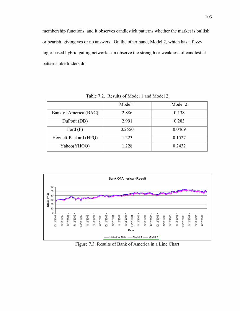
103
membership functions, and it observes candlestick patterns whether the market is bullish
or bearish, giving yes or no answers. On the other hand, Model 2, which has a fuzzy
logic-based hybrid gating network, can observe the strength or weakness of candlestick
patterns like traders do.
Table 7.2. Results of Model 1 and Model 2
Model 1 Model 2
Bank of America (BAC) 2.886 0.138
DuPont (DD) 2.991 0.283
Ford (F) 0.2550 0.0469
Hewlett-Packard (HPQ) 1.223 0.1527
Yahoo(YHOO) 1.228 0.2432
Bank Of America - Result
0
10
20
30
40
50
60
10/1
2/2
001
1/1
2/2
002
4/1
2/2
002
7/1
2/2
002
10/1
2/2
002
1/1
2/2
003
4/1
2/2
003
7/1
2/2
003
10/1
2/2
003
1/1
2/2
004
4/1
2/2
004
7/1
2/2
004
10/1
2/2
004
1/1
2/2
005
4/1
2/2
005
7/1
2/2
005
10/1
2/2
005
1/1
2/2
006
4/1
2/2
006
7/1
2/2
006
10/1
2/2
006
1/1
2/2
007
4/1
2/2
007
7/1
2/2
007
Date
Sto
ck P
rice
Historical Data Model 1 Model 2
Figure 7.3. Results of Bank of America in a Line Chart

104
Bank of America: March 1, 2006 - June 30, 2006
0
10
20
30
40
50
60
3/1/
2006
3/8/
2006
3/15
/2006
3/22
/2006
3/29
/2006
4/5/
2006
4/12
/2006
4/19
/2006
4/26
/2006
5/3/
2006
5/10
/2006
5/17
/2006
5/24
/2006
5/31
/2006
6/7/
2006
6/14
/2006
6/21
/2006
6/28
/2006
Date
Pri
ce
Historical Price Model 1 Model 2
Figure 7.4. Results in a Line Chart between March 1, 2006, and June 28, 2006
When the market does not display much movement, both models produce
smoother lines. However, Model 1, the simple, gating network-based model, still
produces a slightly rougher line movement. Figure 7.5 shows the results of the two
models for Bank of America from April 20, 2006, to May 19, 2006. During this period,
there was no significant movement in the market, and both models performed fairly well.
However, Model 2 produced a smoother curve line than Model 1. Figure 7.6 shows the
candlestick chart for the same period.
Closer observation reveals slight movement of the line in the result of Model 1
around April 28, 2006 (Figure 7.5). When x = 20 in Figure 7.6, a few black candlesticks
appeared, and Model 1 considered this to be significant. The black candlestick is a sign
of bearish market conditions. Due to this black candlestick pattern, Model 1 determined
the stock price to be falling and sent its decision to the experts to generate the final

105
output. However, one large, white candlestick also appeared in the middle of the run of
black candlesticks. Model 2 took this white candlestick appearance into account when
generating the forecasting prices. The white candlestick is a sign of a bullish market
condition. Therefore, the forecasting data of Model 1 is lower than that of Model 2 after
April 30, 2006. As shown in Figure 7.5, the forecasting price result from Model 1 did
not show an upward trend in movement until a few white candlesticks appeared at the
beginning of May, x = 30 in Figure 13.
Bank Of America Result: April 20, 2006 - May 19, 2006
0
10
20
30
40
50
60
4/20
/2006
4/22
/2006
4/24
/2006
4/26
/2006
4/28
/2006
4/30
/2006
5/2/
2006
5/4/
2006
5/6/
2006
5/8/
2006
5/10
/2006
5/12
/2006
5/14
/2006
5/16
/2006
5/18
/2006
Date
Pri
ce
Historical Price Model 1 Model 2
Figure 7.5. Results in a Line Chart between April 20, 2006, and May 19, 2006
As illustrated in Figure 7.7, Model 1 was not stable, and the forecasted price line
moved up and down rapidly. On the other hand, Model 2 demonstrated a smooth price
movement, and the forecasted price line moved along the actual historical data. Model 1,
the simple, gating network-based model, cannot see the relative size of candlesticks well.

106
Also, the simple gating network makes YES or NO type crisp decisions, so there is less
flexibility. Therefore, Model 1’s simple gating network cannot send ambiguous weight
decisions to the experts, so the overall output is far from the actual historical prices.
Figure 7.6. Candlestick Chart (Bank of America) between April 20, 2006, and May 19,
2006
Model 2, the hybrid gating network-based model, however, can see the relative
sizes of candlesticks and generate flexible decisions due to its use of fuzzy membership
functions. The membership functions control the weight decisions from the gating
network based on the relative size of the candlestick patterns. For example, the relatively
large, white candlestick, which appeared around x = 10 in Figure 7.8, became a bullish
sign, and Model 2 decided that the stock price could go up. Several white candlesticks
appeared after x=10 in Figure 7.8. However, the black candlestick and the doji
candlestick, which appeared between x=10 and x=20 in Figure 15, show the hesitation of
the stock prices, and the fuzzy logic-based gating network decided not to raise the stock
price any further. The fuzzy membership function considers the black candlestick to be a

107
negative sign in regards to stock price movement. However, the black candlestick is not
significantly large. Therefore, the hybrid gating network did not decide that the stock
price was falling and did not send ―a stock price is going down‖ decision to the experts.
Actually, the hybrid gating network sent the decision ―the stock price might have a
chance of going down‖ to the experts.
Bank of America: March 1, 2006 - March 31, 2006
40
41
42
43
44
45
46
47
48
3/1/
2006
3/3/
2006
3/5/
2006
3/7/
2006
3/9/
2006
3/11
/2006
3/13
/2006
3/15
/2006
3/17
/2006
3/19
/2006
3/21
/2006
3/23
/2006
3/25
/2006
3/27
/2006
3/29
/2006
3/31
/2006
DAta
Pri
ce
Historical Data Model 1 Model 2
Figure 7.7. Results in a Line Chart between March 1, 2006, and March 31, 2006

108
Figure 7.8. Candlestick Chart (Bank of America) between March 1, 2006, and March 31,
2006
7.3. MODEL 3
7.3.1. Model 3 Results. The results from Model 3 and Model 2, in mean squared
error, are shown in Table 7.3. Model 3 produced better results than Model 2, and the
results fall into satisfactory ranges.
Table 7.3. Results of Model 2 and Model 3
Model 2 Model 3
Bank of America (BAC) 0.9358 0.8235
General Electric (GE) 0.2144 0.1918
Google (GOOG) 83.85 80.92
Monsanto (MON) 4.963 4.634
Toyota (TM) 2.293 2.215

109
7.3.2. Model 3 Review. Figure 7.9 shows the candlestick chart of General
Electric between August 2, 2010, and September 28, 2010. The y-axis represents the
price, and the x-axis represents the trading date. Between x=40 and x=50, a morning star
candlestick pattern appears. This represents a market reversal pattern. Figure 7.10 shows
the line chart of actual historical quotes and the forecasting prices generated by Models 2
and 3. As indicated in Figure 7.10, Model 3 identified the morning star candlestick
pattern and reacted accordingly. Table 7.4 shows the forecasting results of both Models 2
and 3 for General Electric during the same time period, between August 2, 2010, and
September 28, 2010. Model 3, an interval type-2 fuzzy logic system-based model,
produced better results than Model 2, a type-1 fuzzy logic system-based model.
Figure 7.9. Candlestick Chart (General Electric) between August 2, 2010, and September
28, 2010

110
13
13.5
14
14.5
15
15.5
16
16.5
17
8/2/
2010
8/9/
2010
8/16
/201
0
8/23
/201
0
8/30
/201
0
9/6/
2010
9/13
/201
0
9/20
/201
0
Date
Pri
ce ($
)
Historical Type-1 Type-2
Figure 7.10. Price Movement of General Electric between August 2, 2010, and
September 28, 2010
Table 7.4. Results of General Electric between August 2, 2010, and
September 28, 2010
Type-2 Fuzzy Logic System
Type-1 Fuzzy Logic
System
General Electric(GE)
0.0158 0.0413
The period between August 2, 2010, and September 28, 2010, was selected for the
investigation because of the appearance of a morning star candlestick pattern.
Membership functions of type-1 fuzzy logic are crisp. Therefore, Model 2 could not
recognize the small, white candlestick pattern that appeared between x=40 and x=50.
Model 3 tracked the trend of the market during this time period as a downward trend.
When a large, white candlestick pattern appeared just before x=50, it checked the

111
candlestick patterns backward to see if this pattern had any meaning. Model 3 identified
a small, white candlestick pattern on a previous day as a star candlestick pattern. Also,
just before the appearance of this star candlestick pattern, there was a black candlestick.
So, Model 3 checked the overall relationships of these candlestick patterns and market
trends to decide that there was a morning star candlestick pattern in this time period, and
it adjusted the forecasting price.

112
8. CONCLUSIONS
This research explores computational financial forecasting using the candlestick
pattern technique to represent qualitative forecasting. Fuzzy associative memories
manage the ambiguous definitions of candlestick patterns for forecasting. The results
indicate that candlestick pattern technique-based forecasting works better than traditional
forecasting that has been studied and modeled in practice. This research will serve as a
foundation for future studies of computational financial forecasting using the Japanese
candlestick technique.
This dissertation filled gaps in the literature pertaining to understanding
qualitative representations of financial forecasting that uses the candlestick chart
technique and implementing a process of representing the qualitative information of
candlestick patterns using fuzzy associative memories. This research contributes to the
literature by exploring how fuzzy associative memories represent ambiguous candlestick
pattern definitions and influence the model’s performance.
Li’s research presented in Financial Prediction and Trading via Reinforcement
Learning and Soft Computing (2005) discussed quantitative statement-based financial
forecasting systems that help investors make decisions. Chavaranakul’s financial
research, The Development of Hybrid Intelligent Systems for Technical Analysis-Based
Equivolume Charting (2007), used a volume adjusted moving average, neuro-fuzzy-
based genetic algorithm to improve trading performance. Both Li and Chavaranakul’s
studies contain qualitative decision-making procedures, and their findings indicate that
quantitative representation can improve financial forecasting decisions. However, their
studies do not discuss the candlestick chart technique, which also represents financial

113
forecasting qualitatively. Therefore, this dissertation becomes the first introduction of a
candlestick pattern technique-based approach to represent computational financial
forecasting qualitatively.
The qualitative approach was accomplished with fuzzy associative memories
representing candlestick pattern definitions. The forecasting results given by the fuzzy
associative memories can all be expressed qualitatively, such as stock prices rising,
falling, and remaining neutral. The qualitative representation basis of this model does not
tell the exact price changes of stocks, and these qualitative results are not practical for
comparing the performance of different models. Therefore, the qualitative results were
defuzzified to produce quantitative results for comparison purposes.
An additional point related to fuzzy associative memories surrounds the types of
fuzzy membership functions involved. Based on a finding of the final proposed model
consisting of type-2 fuzzy membership functions, higher-order fuzzy membership
functions recognized candlestick patterns better than lower-order fuzzy membership
functions, such as type-1 fuzzy membership functions, which could not detect complex
candlestick patterns well.
This dissertation also makes the following contributions to the literature:
Discussions of the fundamental issues in traditional time series-based
financial forecasting and neural network-based financial forecasting that
led to this research.
Comprehensive descriptions and definitions of candlestick patterns that
can be used for real-world financial forecasting situations.

114
A new, systematic approach for constructing a fuzzy logic system-based
forecasting model with committee machine architecture.
A study of HAVNET-based pattern recognition software usage for
candlestick pattern recognition and comments.
Establishment of fuzzy associative memories that represent ambiguous
candlestick pattern definitions in qualitative representations. Linguistic
values represent the visual appearances of candlestick patterns and charts,
such as ―long real body,‖ ―small real body,‖ ―medium-length upper
shadow line,‖ ―short-length lower shadow line,‖ and so on.
The current investigation was limited by the knowledge and expertise regarding
the representation of candlestick pattern definitions from available publications. The
authors of those publications are real financial traders. However, there are many other
investment traders and experts of candlestick chart techniques. Their individual opinions
and views toward the interpretation of and financial strategies benefitting from the
candlestick chart technique are not reflected in this research. The proposed model is
designed to present the standardized, candlestick pattern definition-based forecasting
systems. However, the model is flexible and adaptable to those individual perspectives.
In addition, the proposed models are for forecasting the next day’s stock prices. The use
of candlestick pattern techniques for other financial products and long-term financial
investment is not examined because the models must be examined in a controlled
environment for comparison purposes. Therefore, it is recommended that further
research be undertaken in these areas as well.

115
The following recommendations for further research are based on the findings of
this study:
Research Validation with Models for Real-World Settings. The
models developed in this research are examined and evaluated with the
fuzzy associative memories and rules developed from publications related
to the use of the candlestick chart technique for investment. Real stock
traders and investors may have different views, knowledge, and
experiences than those discussed in these publications. Therefore, it is
interesting to evaluate those real-world financial investors’ and traders’
expertise and knowledge through fuzzy associative memory and rules.
The models developed in this study are flexible and adaptive so that
differences in their strategies and rules can be managed. The broad views
and knowledge of type-2 fuzzy membership functions are particularly
adaptable.
Extension of Type-2 Fuzzy Logic. The extensive research regarding
interpretations of candlestick patterns using general type-2 fuzzy logic is
interesting because the proposed model was limited to processes with
interval type-2 fuzzy logic-based secondary membership functions. This
technique can be extended to higher-order general type-2 fuzzy
membership functions. The general type-2 fuzzy membership functions
provide broad flexibility in interpreting not only candlestick pattern
definitions but also the rules and knowledge that real-world investors and
stock traders apply to their own investment strategies.

116
Type-2 fuzzy membership functions handle ambiguity and
uncertainty well because the membership functions have multi-
dimensional spaces. More research is required to determine the
appropriate parameters for standard deviations and mean values. If the
multi-dimensional spaces are too wide, then the results could remain
undetermined. If the spaces are too narrow, then there could be no
difference between type-1 and type-2 membership functions.
Higher-Order Committee Machines. One feature of committee
machines that is useful for managing issues of large data sets is that they
can divide a large system into smaller systems to solve a complex
problem. Candlestick pattern recognition is controlled by one large
system in the current research. Dividing this large system into smaller
systems is interesting but challenging work, especially when general type-
2 fuzzy membership functions are introduced to represent the ambiguous
definitions of candlestick patterns, which requires searching for
appropriate algorithms for combining small, partitioned systems.
Japanese Candlestick Chart Techniques for Other Financial
Products. Current research reveals that the Japanese candlestick chart
technique works well for daily stock price forecasting. However, no study
investigates forecasting other financial products with candlestick chart
techniques. The potential use of candlestick chart techniques to forecast
foreign stock exchange markets, stock option markets, and foreign
currency exchange markets should be explored. The change of forecasting

117
areas would necessitate changing the time frames of candlesticks because
other financial products require different investment strategies. For the
currency exchange market, day trading is the popular approach, and it
prefers minute-based candlestick charts for trading strategies. On the
other hand, long-term investment management prefers multi-day, weekly,
and monthly candlestick charts for forecasting stock prices.
Computational financial forecasting using the candlestick pattern technique is still
new. Much research in relevant areas must still be conducted to study financial
forecasting with this Japanese candlestick chart technique.

118
APPENDIX A.
MATLAB SCRIPTS FOR MAIN DATA FLOW TRANSACTION PROGRAM

119
clear all;
%%%%%%%%%%%%%%%%%%%%%%%%%%%%%%%%%%%%%%%%%%%
%%% Selecting an Excel File and Channel the file with MATLAB %%%
%%%%%%%%%%%%%%%%%%%%%%%%%%%%%%%%%%%%%%%%%%%
File = 'appl1.xls';
%%%%%%%%%%%%%%%%%%%%%%%%%%%%%%%%%%%%%%%%%%%
channel = ddeinit('excel',File);
%%%%%%%%%%%%%%%%%%%%%%%%%%%%%%%%%%%%%%%%%%%
%%% Each Columns of EXCEL %%%
%%%%%%%%%%%%%%%%%%%%%%%%%%%%%%%%%%%%%%%%%%%
% col 1 = Date
% col 2 = Open price
% col 3 = High price
% col 4 = Low price
% col 5 = Close price
% col 6 = trading volume
% row 1 & 2 = Label
% row 3 = data starts
%%%%%%%%%%%%%%%%%%%%%%%%%%%%%%%%%%%%%%%%%%%
%%% Numbers of DATA (Not Input) %%%
%%%%%%%%%%%%%%%%%%%%%%%%%%%%%%%%%%%%%%%%%%%
num_start = 2;
num_end = 50; %original 504
num_row = num_end - num_start;
num_input = 5;
% Last row = End of the data = 600
% the number of row = 600-2 = 598
avg_can = 3; % this number must be less than num_input
% numbers of candles used for averaging
%%%%%%%%%%%%%%%%%%%%%%%%%%%%%%%%%%%%%%%%%%%
%%% Retreive the DATA
%%%%%%%%%%%%%%%%%%%%%%%%%%%%%%%%%%%%%%%%%%%
Data = ddereq(channel,'r2c2:r1000c6'); %% always check the size

120
Open = Data(1:num_row,1);
High = Data(1:num_row,2);
Low = Data(1:num_row,3);
Close = Data(1:num_row,4);
Vol = Data(1:num_row,5);
% All Combined Matrix
A = [Open High Low Close Vol];
%%%%%%%%%%%%%%%%%%%%%%%%%%%%%%%%%%%%%%%%%%%
%%% For Finding Candlestick Elements
%%%%%%%%%%%%%%%%%%%%%%%%%%%%%%%%%%%%%%%%%%%
[Body_Size, Color, Doji, C_of_RB]= Candle_Basic(Open,Close,num_row);
Body_Size;
Body_Size = abs(Body_Size);
Color;
Doji;
C_of_RB;
%# of data checking: = # of data should be the same as # of "num_row"
%num_Body_Size = size(Body_Size); % checking the size of array
%%%%% previous setting
% Candle_Size;
% Candle_Size = abs(Candle_Size);
% Color;
% Doji;
% Table_Candle_Basic = [Body_Size Color C_of_RB];
[Up_Shadow_L, Low_Shadow_L, C_of_Up_Shadow, C_of_Low_Shadow] ...
= Shadow_Basic(Open,High,Low,Close,Body_Size,num_row);
Up_Shadow_L;
Low_Shadow_L;
C_of_Up_Shadow;
C_of_Low_Shadow;
%# of data checking: = # of data should be the same as # of "num_row"
%num_Up_Shadow_L = size(Up_Shadow_L);
% Table_Shadow_Basic ...
% = [Up_Shadow_L Low_Shadow_L C_of_Up_Shadow C_of_Low_Shadow];
%%%%%%%%%%%%%%%%%%%%%%%%%%%%%%%%%%%%%%%%%%%

121
%%%% Market Trend Line
%%%%%%%%%%%%%%%%%%%%%%%%%%%%%%%%%%%%%%%%%%%
%
% This market trend line is calculated from the day before forecasting
% day. In other words, if the forecasting day is A, then trend line is
% from day (A-1). Trend_5 is calculated based on days of (A-1, A-2,
% A-3, A-4, and A-5), Trend_3 is w/ days of (A-1, A-2, and A-3).
% Trend line is good at checking the average movement of the price.
% Not the same as Moving Average (MA)
[C_Trend_2, C_Trend_3, C_Trend_4, C_Trend_5, ...
O_Trend_2, O_Trend_3, O_Trend_4, O_Trend_5, ...
C_of_RB_Trend_2, C_of_RB_Trend_3, C_of_RB_Trend_4, C_of_RB_Trend_5] ...
= Trend_Basic(Open, Close, C_of_RB, num_row);
C_Trend_2;
C_Trend_3;
C_Trend_4;
C_Trend_5;
O_Trend_2;
O_Trend_3;
O_Trend_4;
O_Trend_5;
C_of_RB_Trend_2;
C_of_RB_Trend_3;
C_of_RB_Trend_4;
C_of_RB_Trend_5;
%# of data checking: = # of data should be the same as # of "num_row"
% num_C_Trend_2 = size(C_Trend_2);
% num_C_Trend_3 = size(C_Trend_3);
% num_C_Trend_4 = size(C_Trend_4);
% num_C_Trend_5 = size(C_Trend_5);
% Table_C_Trend_Basic = [C_Trend_2 C_Trend_3 C_Trend_4 C_Trend_5];
% Table_O_Trend_Basic = [O_Trend_2 O_Trend_3 O_Trend_4 O_Trend_5];
% Table_C_of_RB_Trend_Basic = ...
% [C_of_RB_Trend_2 C_of_RB_Trend_3 C_of_RB_Trend_4 C_of_RB_Trend_5];
%%%%%%%%%%%%%%%%%%%%%%%%%%%%%%%%%%%%%%%%%%%
%%%% Market Trend Line ID (Positive or Negative)
%%%%%%%%%%%%%%%%%%%%%%%%%%%%%%%%%%%%%%%%%%%
% [C_Trend_ID, C_of_RB_ID] = Trend_ID(num_row, Close, C_of_RB);

122
%
% C_Trend_ID;
% C_of_RB_ID;
%%%%%%%%%%%%%%%%%%%%%%%%%%%%%%%%%%%%%%%%%%%
%%%% Checking Up Trend based on closing price (positive trend - upward)
[Up_Close_Trend_3, Up_Close_Trend_4, Up_Close_Trend_5, ...
Up_Close_Trend_6, Up_Close_Trend_7] ...
= Trend_Close_Up(num_row, Close);
Up_Close_Trend_3;
Up_Close_Trend_4;
Up_Close_Trend_5;
Up_Close_Trend_6;
Up_Close_Trend_7;
%size(Up_Close_Trend_3)
%size(Up_Close_Trend_4)
%size(Up_Close_Trend_5)
%size(Up_Close_Trend_6)
%size(Up_Close_Trend_7)
%%% Test
%Table_Close_Trend = [Up_Close_Trend_3 Up_Close_Trend_4]
%%%%%%%%%%%%%%%%%%%%%%%%%%%%%%%%%%%%%%%%%%%
%%%% Checking Up Trend based on closing price (Negative trend - downward)
[Down_Close_Trend_3, Down_Close_Trend_4, Down_Close_Trend_5, ...
Down_Close_Trend_6, Down_Close_Trend_7] ...
= Trend_Close_Down(num_row, Close);
Down_Close_Trend_3;
Down_Close_Trend_4;
Down_Close_Trend_5;
Down_Close_Trend_6;
Down_Close_Trend_7;
%size(Down_Close_Trend_3)
%size(Down_Close_Trend_4)
%size(Down_Close_Trend_5)
%size(Down_Close_Trend_6)
%size(Down_Close_Trend_7)
%%% Test

123
%Table_Close_Trend = [Up_Close_Trend_3 Up_Close_Trend_4]
%%%%%%%%%%%%%%%%%%%%%%%%%%%%%%%%%%%%%%%%%%%
%%%% Checking Up Trend based on center of real body (CRB)
%%%% Positive trend (upward trend)
[Up_C_RB_Trend_3, Up_C_RB_Trend_4, Up_C_RB_Trend_5, ...
Up_C_RB_Trend_6, Up_C_RB_Trend_7] = Trend_C_RB_Up(num_row, C_of_RB);
Up_C_RB_Trend_3;
Up_C_RB_Trend_4;
Up_C_RB_Trend_5;
Up_C_RB_Trend_6;
Up_C_RB_Trend_7;
% size(Up_C_RB_Trend_3)
% size(Up_C_RB_Trend_4)
% size(Up_C_RB_Trend_5)
% size(Up_C_RB_Trend_6)
% size(Up_C_RB_Trend_7)
%%%%%%%%%%%%%%%%%%%%%%%%%%%%%%%%%%%%%%%%%%%
%%%% Checking Up Trend based on center of real body (CRB)
%%%% Negative trend (downward trend)
[Down_C_RB_Trend_3, Down_C_RB_Trend_4, Down_C_RB_Trend_5, ...
Down_C_RB_Trend_6, Down_C_RB_Trend_7] ...
= Trend_C_RB_Down(num_row, C_of_RB);
Down_C_RB_Trend_3;
Down_C_RB_Trend_4;
Down_C_RB_Trend_5;
Down_C_RB_Trend_6;
Down_C_RB_Trend_7;
% size(Down_C_RB_Trend_3)
% size(Down_C_RB_Trend_4)
% size(Down_C_RB_Trend_5)
% size(Down_C_RB_Trend_6)
% size(Down_C_RB_Trend_7)
%%%%%%%%%%%%%%%%%%%%%%%%%%%%%%%%%%%%%%%%%%%
%%%% Moving Average for Closing Price per body size
[Avg_Body_Size_3, Avg_Body_Size_4, Avg_Body_Size_5, ...
Avg_Body_Size_6, Avg_Body_Size_7, MA_Close_3, MA_Close_4, ...

124
MA_Close_5, MA_Close_6, MA_Close_7, MA_Close_3_Dir, ...
MA_Close_4_Dir, MA_Close_5_Dir, MA_Close_6_Dir, MA_Close_7_Dir] ...
= MA_Close(num_row, Close, Body_Size);
Avg_Body_Size_3;
Avg_Body_Size_4;
Avg_Body_Size_5;
Avg_Body_Size_6;
Avg_Body_Size_7;
MA_Close_3;
MA_Close_4;
MA_Close_5;
MA_Close_6;
MA_Close_7;
MA_Close_3_Dir;
MA_Close_4_Dir;
MA_Close_5_Dir;
MA_Close_6_Dir;
MA_Close_7_Dir;
% size(Avg_Body_Size_4);
% size(MA_Close_4);
% size(MA_Close_7_Dir);
%%%%%%%%%%%%%%%%%%%%%%%%%%%%%%%%%%%%%%%%%%%
%%%% Moving Average for Center of real body Price per body size
[MA_C_RB_3, MA_C_RB_4, MA_C_RB_5, MA_C_RB_6, MA_C_RB_7,
MA_C_RB_3_Dir, ...
MA_C_RB_4_Dir, MA_C_RB_5_Dir, MA_C_RB_6_Dir, MA_C_RB_7_Dir] ...
= MA_C_RB(num_row, C_of_RB, Body_Size);
MA_C_RB_3;
MA_C_RB_4;
MA_C_RB_5;
MA_C_RB_6;
MA_C_RB_7;
MA_C_RB_3_Dir;
MA_C_RB_4_Dir;
MA_C_RB_5_Dir;
MA_C_RB_6_Dir;
MA_C_RB_7_Dir;

125
% size(MA_C_RB_7)
% size(MA_C_RB_7_Dir)
%%%%%%%%%%%%%%%%%%%%%%%%%%%%%%%%%%%%%%%%%%%
%%%% Candlestick Pattern Identification Section
%%%%%%%%%%%%%%%%%%%%%%%%%%%%%%%%%%%%%%%%%%%
%%%%%%%%%%%%%%%%%%%%%%%%%%%%%%%%%%%%%%%%%%%
%%%% Basic Candlestick Identification
%%%%%%%%%%%%%%%%%%%%%%%%%%%%%%%%%%%%%%%%%%%
%% Body_Ratio is for checking if the candlestick is long or short
%% 4 day average body size (devided by 4 days data)
[Avg_Body_Size, Body_Ratio, Body_Ratio_12, Avg_Body_Size10, ...
Body_Ratio10]= Body_Ratio(num_row, Body_Size);
Avg_Body_Size;
Body_Ratio;
Body_Ratio_12;
Avg_Body_Size10;
Body_Ratio10;
% size(Body_Ratio10);
%# of data checking: = # of data should be the same as # of "num_row"
% num_Body_Ratio = size(Body_Ratio)
%%%%%%%%%%%%%%%%%%%%%%%%%%%%%%%%%%%%%%%%%%%
%% Shadow_Ratio is for checking if the candlestick has long shadows or
%% short shadows.
%% 4 days Average (divided by 4 days data)
[Avg_Up_Shadow_L, Avg_Low_Shadow_L, Up_Shadow_Ratio, ...
Low_Shadow_Ratio, Up_Low_Shadow_Ratio, Low_Up_Shadow_Ratio]= ...
Shadow_Ratio(num_row, Up_Shadow_L, Low_Shadow_L);
Avg_Up_Shadow_L;
Up_Shadow_Ratio;
Avg_Low_Shadow_L;
Low_Shadow_Ratio;
Up_Low_Shadow_Ratio;
Low_Up_Shadow_Ratio;
% b = size(Up_Low_Shadow_Ratio)

126
%# of data checking: = # of data should be the same as # of "num_row"
% num_Up_Shadow_Ratio = size(Up_Shadow_Ratio)
% table format for testing
% a = [Up_Low_Shadow_Ratio Low_Up_Shadow_Ratio];
%%%%%%%%%%%%%%%%%%%%%%%%%%%%%%%%%%%%%%%%%%%
%% Body_Shadow_Ratio is for checking the balance of candlestick upper
%% shadow and lower shadow and real body
[U_Shadow_Body_Ratio, L_Shadow_Body_Ratio, ...
U_Shadow_Avg_Body_Ratio, L_Shadow_Avg_Body_Ratio] = ...
Shadow_Body_Ratio(num_row, Up_Shadow_L, Low_Shadow_L, Body_Size, ...
Color, Avg_Body_Size);
U_Shadow_Body_Ratio;
L_Shadow_Body_Ratio;
U_Shadow_Avg_Body_Ratio;
L_Shadow_Avg_Body_Ratio;
% table format for testing
% a = [Up_Shadow_L Body_Size U_Shadow_Body_Ratio
U_Shadow_Avg_Body_Ratio];
%# of data checking: = # of data should be the same as # of "num_row"
%num_U_Shadow_Body_Ratio = size(U_Shadow_Body_Ratio)
% checking the size of array
% Table_Shadow_Body_Ratio = ...
% [U_Shadow_Body_Ratio L_Shadow_Body_Ratio ...
% U_Shadow_Avg_Body_Ratio L_Shadow_Avg_Body_Ratio];
%%%%%%%%%%%%%%%%%%%%%%%%%%%%%%%%%%%%%%%%%%%
%%%% Single Candlestick Identification
%%%%%%%%%%%%%%%%%%%%%%%%%%%%%%%%%%%%%%%%%%%
%%%%%%%%%%%%%%%%%%%%%%%%%%%%%%%%%%%%%%%%%%%
%% MaruBozu Candlestick Pattern - Identification - Fuzzy
[Marubozu_rate] = Marubozu_Fuzz(num_row, U_Shadow_Avg_Body_Ratio, ...
L_Shadow_Avg_Body_Ratio, Body_Ratio);
Marubozu_rate;
% size(Marubozu_rate)

127
% for testing
% body_table = [Body_Ratio Up_Shadow_L Low_Shadow_L Marubozu_rate];
%%%%%%%%%%%%%%%%%%%%%%%%%%%%%%%%%%%%%%%%%%%
%% Closing Marubozu
[C_Marubozu_rate] = C_Marubozu_Fuzz(num_row, U_Shadow_Avg_Body_Ratio, ...
L_Shadow_Avg_Body_Ratio, Color, Body_Ratio);
C_Marubozu_rate;
% body_table = [Color Body_Ratio Up_Shadow_L Low_Shadow_L C_Marubozu_rate];
%%%%%%%%%%%%%%%%%%%%%%%%%%%%%%%%%%%%%%%%%%%
%% Opening Marubozu
[O_Marubozu_rate] = O_Marubozu_Fuzz(num_row, U_Shadow_Avg_Body_Ratio, ...
L_Shadow_Avg_Body_Ratio, Color, Body_Ratio);
O_Marubozu_rate;
% body_table = [Color Body_Ratio Up_Shadow_L Low_Shadow_L O_Marubozu_rate];
%%%%%%%%%%%%%%%%%%%%%%%%%%%%%%%%%%%%%%%%%%%
%% Spinning Top (Koma)
%
[Spin_Tops_rate] = Spin_Tops_Fuzz(num_row, Up_Shadow_L, ...
Low_Shadow_L, Body_Ratio, Body_Size);
Spin_Tops_rate;
% body_table = [Color Up_Shadow_L Low_Shadow_L Body_Size Body_Ratio ...
% Spin_Tops_rate];
%%%%%%%%%%%%%%%%%%%%%%%%%%%%%%%%%%%%%%%%%%%
%% Doji - All types of Doji Patterns including
%% Long Legged Doji, Gravestone Doji, and Dragonfly Doji
[Long_Leg_Doji_rate, Gravestone_Doji_rate, Dragonfly_Doji_rate] = ...
Doji_fuzz(num_row, Body_Ratio, Up_Shadow_Ratio, Low_Shadow_Ratio);
Long_Leg_Doji_rate;
Gravestone_Doji_rate;
Dragonfly_Doji_rate;
%ignore the first 4 numbers(outputs)

128
%%%%%%%%%%%%%%%%%%%%%%%%%%%%%%%%%%%%%%%%%%%
%% Paper Umbrella
[Paper_Umbrella_rate] = Paper_Umbrella_fuzz(num_row, Body_Ratio, ...
L_Shadow_Body_Ratio);
Paper_Umbrella_rate;
% Avg_Up_Shadow_L;
% Up_Shadow_Ratio;
% Avg_Low_Shadow_L;
% Low_Shadow_Ratio;
% Up_Low_Shadow_Ratio;
% Low_Up_Shadow_Ratio;
%
% Up_Shadow_L;
% Low_Shadow_L;
% Up_Low_Shadow_Ratio;
% Low_Up_Shadow_Ratio;
%%%% for testing purpose, all below commented
%%%%%%%%%%%%%%%%%%%%%%%%%%%%%%%%%%%%%%%%%%%
%% MULTIPLE-COMBO CANDLESTICK PATTERNS
%%%%%%%%%%%%%%%%%%%%%%%%%%%%%%%%%%%%%%%%%%%
%%%%%%%%%%%%%%%%%%%%%%%%%%%%%%%%%%%%%%%%%%%
%% Engulfing Patterns
[Engluf_Down_fuzz_rate] = Engulf_Down_fuzz(num_row, Color, Body_Size, ...
Open, Close, Body_Ratio_12, ...
Down_C_RB_Trend_6, Down_C_RB_Trend_7, MA_C_RB_6_Dir,
MA_C_RB_7_Dir);
Engluf_Down_fuzz_rate;
% %size(Engluf_Down_fuzz_rate)
[Engluf_Up_fuzz_rate] = Engulf_Up_fuzz(num_row, Color, Body_Size, ...
Open, Close, Body_Ratio_12, ...
Up_C_RB_Trend_6, Up_C_RB_Trend_7, MA_C_RB_6_Dir, MA_C_RB_7_Dir);
Engluf_Up_fuzz_rate;
%size(Engluf_Up_fuzz_rate);

129
%%%%%%%%%%%%%%%%%%%%%%%%%%%%%%%%%%%%%%%%%%%
%% Piercing Patterns
[Piercing_fuzz_rate] = Piercing_fuzz(num_row, Color, Body_Size, ...
Open, Close, Low, C_of_RB, Body_Ratio, Body_Ratio10, ...
Down_C_RB_Trend_6, Down_C_RB_Trend_7, MA_C_RB_6_Dir,
MA_C_RB_7_Dir);
Piercing_fuzz_rate;
size(Piercing_fuzz_rate);
%%%%%%%%%%%%%%%%%%%%%%%%%%%%%%%%%%%%%%%%%%%
%% Dark Cloud Cover Patterns
[Dark_Cloud_fuzz_rate] = Dark_Cloud_fuzz(num_row, Color, Body_Size, ...
Open, Close, High, C_of_RB, Body_Ratio, Body_Ratio10, ...
Up_C_RB_Trend_6, Up_C_RB_Trend_7, MA_C_RB_6_Dir, MA_C_RB_7_Dir);
Dark_Cloud_fuzz_rate;
% size(Dark_Cloud_fuzz_rate);
%%%%%%%%%%%%%%%%%%%%%%%%%%%%%%%%%%%%%%%%%%%
%% Morning_Star Patterns
[Morning_Star_fuzz_rate] = Morning_Star_fuzz(num_row, Color, ...
Body_Size, Open, Close, Low, C_of_RB, Body_Ratio_12, ...
Body_Ratio, Body_Ratio10, ...
Down_C_RB_Trend_6, Down_C_RB_Trend_7, MA_C_RB_6_Dir,
MA_C_RB_7_Dir);
Morning_Star_fuzz_rate;
%size(Morning_Star_fuzz_rate);
%%%%%%%%%%%%%%%%%%%%%%%%%%%%%%%%%%%%%%%%%%%
%% Evening Star Patterns
[Evening_Star_fuzz_rate] = Evening_Star_fuzz(num_row, Color, ...
Body_Size, Open, Close, Low, C_of_RB, Body_Ratio_12, ...
Body_Ratio, Body_Ratio10, ...
Up_C_RB_Trend_6, Up_C_RB_Trend_7, MA_C_RB_6_Dir, MA_C_RB_7_Dir);
Evening_Star_fuzz_rate;

130
% size(Evening_Star_fuzz_rate);
%%%%%%%%%%%%%%%%%%%%%%%%%%%%%%%%%%%%%%%%%%%
%% White Solders Patterns
[White_Soldiers_fuzz_rate] = White_Soldiers_fuzz(num_row, Color, ...
Body_Size, Open, Close, Low, High, C_of_RB, ...
Body_Ratio, Body_Ratio10, Up_Shadow_L, ...
Down_C_RB_Trend_6, Down_C_RB_Trend_7, MA_C_RB_6_Dir,
MA_C_RB_7_Dir);
White_Soldiers_fuzz_rate;
% % size(White_Soldiers_fuzz_rate)
%%%%%%%%%%%%%%%%%%%%%%%%%%%%%%%%%%%%%%%%%%%
%% Black Crows Patterns
[Black_Crows_fuzz_rate] = Black_Crows_fuzz(num_row, Color, ...
Body_Size, Open, Close, Low, High, C_of_RB, ...
Body_Ratio, Body_Ratio10, Low_Shadow_L, ...
Up_C_RB_Trend_6, Up_C_RB_Trend_7, MA_C_RB_6_Dir, MA_C_RB_7_Dir);
Black_Crows_fuzz_rate;
% size(Black_Crows_fuzz_rate)
%%%%%%%%%%%%%%%%%%%%%%%%%%%%%%%%%%%%%%%%%%%
%%% Prep for combination/weights generation
%%%% when it's up trend (reversal sign from bull to bear)
[wt_B_Marubozu_rate wt_C_B_Marubozu_rate wt_O_B_Marubozu_rate ...
wt_Long_Leg_Doji_rate wt_Gravestone_Doji_rate ...
wt_Dragonfly_Doji_rate wt_Paper_Umbrella_rate ...
wt_Engluf_Up_fuzz_rate wt_Dark_Cloud_fuzz_rate ...
wt_Evening_Star_fuzz_rate wt_Black_Crows_fuzz_rate ...
ct_B_Marubozu_rate ct_C_B_Marubozu_rate ct_O_B_Marubozu_rate ...
ct_Long_Leg_Doji_rate ct_Gravestone_Doji_rate ...
ct_Dragonfly_Doji_rate ct_Paper_Umbrella_rate ...
ct_Engluf_Up_fuzz_rate ct_Dark_Cloud_fuzz_rate ...
ct_Evening_Star_fuzz_rate ct_Black_Crows_fuzz_rate] ...
= wt_bear(num_row, Color, Marubozu_rate, C_Marubozu_rate, ...
O_Marubozu_rate, Long_Leg_Doji_rate, Gravestone_Doji_rate, ...
Dragonfly_Doji_rate, Paper_Umbrella_rate, Engluf_Up_fuzz_rate, ...
Dark_Cloud_fuzz_rate, Evening_Star_fuzz_rate, Black_Crows_fuzz_rate);

131
wt_B_Marubozu_rate;
wt_C_B_Marubozu_rate;
wt_O_B_Marubozu_rate;
wt_Long_Leg_Doji_rate;
wt_Gravestone_Doji_rate;
wt_Dragonfly_Doji_rate;
wt_Paper_Umbrella_rate;
wt_Engluf_Up_fuzz_rate;
wt_Dark_Cloud_fuzz_rate;
wt_Black_Crows_fuzz_rate;
ct_B_Marubozu_rate;
ct_C_B_Marubozu_rate;
ct_O_B_Marubozu_rate;
ct_Long_Leg_Doji_rate;
ct_Gravestone_Doji_rate;
ct_Dragonfly_Doji_rate;
ct_Paper_Umbrella_rate;
ct_Engluf_Up_fuzz_rate;
ct_Dark_Cloud_fuzz_rate;
ct_Black_Crows_fuzz_rate;
% size(wt_Gravestone_Doji_rate);
% size(Dark_Cloud_fuzz_rate);
% size(wt_O_Marubozu_rate);
% size(ct_Gravestone_Doji_rate);
% size(ct_Dark_Cloud_fuzz_rate);
% size(ct_Black_Crows_fuzz_rate);
%%%% when it's down trend (reversal sign from bear to bull)
[wt_W_Marubozu_rate wt_C_W_Marubozu_rate ...
wt_O_W_Marubozu_rate wt_Spin_Tops_rate wt_Engluf_Down_fuzz_rate ...
wt_Piercing_fuzz_rate wt_Morning_Star_fuzz_rate ...
wt_White_Soldiers_fuzz_rate ...
ct_W_Marubozu_rate ct_C_W_Marubozu_rate ct_O_W_Marubozu_rate ...
ct_Spin_Tops_rate ct_Engluf_Down_fuzz_rate ct_Piercing_fuzz_rate ...
ct_Morning_Star_fuzz_rate ct_White_Soldiers_fuzz_rate] ...
= wt_bull(num_row, Color, Marubozu_rate, C_Marubozu_rate, ...
O_Marubozu_rate, Spin_Tops_rate, Engluf_Down_fuzz_rate, ...
Piercing_fuzz_rate, Morning_Star_fuzz_rate, White_Soldiers_fuzz_rate);
wt_W_Marubozu_rate;
wt_C_W_Marubozu_rate;

132
wt_O_W_Marubozu_rate;
wt_Spin_Tops_rate;
wt_Engluf_Down_fuzz_rate;
wt_Piercing_fuzz_rate;
wt_Morning_Star_fuzz_rate;
wt_White_Soldiers_fuzz_rate;
ct_W_Marubozu_rate;
ct_C_W_Marubozu_rate;
ct_O_W_Marubozu_rate;
ct_Spin_Tops_rate;
ct_Engluf_Down_fuzz_rate;
ct_Piercing_fuzz_rate;
ct_Morning_Star_fuzz_rate;
ct_White_Soldiers_fuzz_rate;
% size(wt_O_W_Marubozu_rate);
% size(wt_Engluf_Down_fuzz_rate);
% size(wt_Piercing_fuzz_rate);
% size(wt_Morning_Star_fuzz_rate);
% size(wt_White_Soldiers_fuzz_rate);
% size(ct_C_W_Marubozu_rate);
% size(ct_Morning_Star_fuzz_rate);
% size(ct_White_Soldiers_fuzz_rate);
% size(ct_Spin_Tops_rate);
%%%%%%%%%%%%%%%%%%%%%%%%%%%%%%%%%%%%%%%%%%%
%%%%% forecasting control system
[wt_down wt_up wt_side] = wt_gen(num_row, wt_B_Marubozu_rate, ...
wt_C_B_Marubozu_rate, wt_O_B_Marubozu_rate, ...
wt_Long_Leg_Doji_rate, wt_Gravestone_Doji_rate, ...
wt_Dragonfly_Doji_rate, wt_Paper_Umbrella_rate, ...
wt_Engluf_Up_fuzz_rate, wt_Dark_Cloud_fuzz_rate, ...
wt_Evening_Star_fuzz_rate, wt_Black_Crows_fuzz_rate, ...
ct_B_Marubozu_rate, ct_C_B_Marubozu_rate, ct_O_B_Marubozu_rate, ...
ct_Long_Leg_Doji_rate, ct_Gravestone_Doji_rate, ...
ct_Dragonfly_Doji_rate, ct_Paper_Umbrella_rate, ...
ct_Engluf_Up_fuzz_rate, ct_Dark_Cloud_fuzz_rate, ...
ct_Evening_Star_fuzz_rate, ct_Black_Crows_fuzz_rate, ...
wt_W_Marubozu_rate, wt_C_W_Marubozu_rate, wt_O_W_Marubozu_rate, ...
wt_Spin_Tops_rate, wt_Engluf_Down_fuzz_rate, wt_Piercing_fuzz_rate, ...
wt_Morning_Star_fuzz_rate, wt_White_Soldiers_fuzz_rate, ...
ct_W_Marubozu_rate, ct_C_W_Marubozu_rate, ct_O_W_Marubozu_rate, ...
ct_Spin_Tops_rate, ct_Engluf_Down_fuzz_rate, ct_Piercing_fuzz_rate, ...
ct_Morning_Star_fuzz_rate, ct_White_Soldiers_fuzz_rate, ...

133
Up_C_RB_Trend_6, Up_C_RB_Trend_7, ...
Down_C_RB_Trend_6, Down_C_RB_Trend_7, MA_C_RB_6_Dir,
MA_C_RB_7_Dir);
wt_down;
wt_up;
wt_side;
% size(wt_down)
% size(wt_up)
% size(wt_side)
%%%%%%%%%%%%%%%%%%%%%%%%%%%%%%%%%%%%%%%%%%%
%%%% Neural Networks
%%%%%%%%%%%%%%%%%%%%%%%%%%%%%%%%%%%%%%%%%%%
% For Recurrent Networks
% [RNN_S, RNN_C] = Recurrent(Open, High, Low, Close, Candle_Size, ...
% Color, Doji, num_row, num_input);
%
% For Generalized Regression Neural Networks
[S_GRNN_Result] = S_GRNN(Open, High, Low, Close, Vol, num_row, num_input);
S_GRNN_Result;
% wk1write('GRNN_Result1.wk1',S_GRNN_Result); % Record the GRNN Result
% [GRNN_S, GRNN_C] = S_GRNN(Open, High, Low, Close, Candle_Size, ...
% Color, Doji, num_row, num_input);
% Adaptive Neural Networks
% [Result_Adapt] = Adapt(Open, High, Low, Close, Vol, Candle_Size, Color,...
% Doji);
%
%%%%%%%%%%%%%%%%%%%%%%%%%%%%%%%%%%%%%%%%%%%
%%%% Joining Neural Networks and Candles
%%%%%%%%%%%%%%%%%%%%%%%%%%%%%%%%%%%%%%%%%%%
[Forecast_GRNN Forecast_Data] = ForecastGRNN(num_input, avg_can, ...
S_GRNN_Result, Candle_Size, Color, Doji);

134
Forecast_GRNN;
Forecast_Data;
wk1write('Forecast_GRNN.wk1',Forecast_GRNN);% Record Forecasted GRNN Result
wk1write('Forecast_Data.wk1',Forecast_Data);% Record Forecasted Data
%%%%%%%%%%%%%%%%%%%%%%%%%%%%%%%%%%%%%%%%%%%
%%%% Fuzzy Logic 1
%%%%%%%%%%%%%%%%%%%%%%%%%%%%%%%%%%%%%%%%%%%
[Forecast_Fuzz_comp] = Forecast_Fuzzy_Comp(num_row, S_GRNN_Result, ...
wt_down, wt_up, wt_side);
Forecast_Fuzz_comp;
size(Forecast_Fuzz_comp);
wk1write('Forecast_Fuzz_comp.wk1',Forecast_Fuzz_comp);
% Record Forecasted Data
[Forecast_Data_Fuzz Fuzz_Center_List] ...
= Forecast_Fuzzy_Basic(num_input, avg_can, S_GRNN_Result, ...
Candle_Size, Color, Doji);
Forecast_Data_Fuzz;
Fuzz_Center_List;
wk1write('Forecast_Data_Fuzz.wk1',Forecast_Data_Fuzz);
% Record Forecasted Data
wk1write('Fuzz_Center_List.wk1',Fuzz_Center_List);
% record data
%%%%%%%%%%%%%%%%%%%%%%%%%%%%%%%%%%%%%%%%%%%
%%% Mean Squared Error Report for GRNN
%%%%%%%%%%%%%%%%%%%%%%%%%%%%%%%%%%%%%%%%%%%
[MSE_Forecast_Data MSE_Forecast_GRNN Data_Counter] = Result_Ck(Close, ...
avg_can, Forecast_Data, Forecast_GRNN);
MSE_Forecast_Data;
MSE_Forecast_GRNN;
Data_Counter
wk1write('MSE_Forecast_Data.wk1',MSE_Forecast_Data);
% Record Forecasted GRNN Result
wk1write('MSE_Forecast_GRNN.wk1',MSE_Forecast_GRNN);
% Record Forecasted Data

135
%%%%%%%%%%%%%%%%%%%%%%%%%%%%%%%%%%%%%%%%%%%
%%% Mean Squared Error Report for Fuzzy logic
%%%%%%%%%%%%%%%%%%%%%%%%%%%%%%%%%%%%%%%%%%%
[MSE_Forecast_Fuzz] = Result_Ck_F(Close, avg_can, Forecast_Data_Fuzz);
MSE_Forecast_Fuzz;
wk1write('MSE_Forecast_Fuzz.wk1',MSE_Forecast_Fuzz);
% Record Forecasted Fuzz Result
%%%%%%%%%%%%%%%%%%%%%%%%%%%%%%%%%%%%%%%%%%%
%%% Mean Squared Error Report for Fuzzy logic
%%%%%%%%%%%%%%%%%%%%%%%%%%%%%%%%%%%%%%%%%%%
[MSE_Forecast_Fuzz_Comp] = Result_Ck_F_Comp(Close, avg_can, ...
Forecast_Fuzz_comp);
MSE_Forecast_Fuzz_Comp
size(MSE_Forecast_Fuzz_Comp)
wk1write('MSE_Forecast_Fuzz_Comp.wk1',MSE_Forecast_Fuzz_Comp);
% record data

136
APPENDIX B.
HISTORICAL STOCK PRICE DATA SOURCES

137
Model 1 Experiment Data References
Exxon Mobil (XOM): April 15, 2002 through March 31, 2006.
http://finance.yahoo.com/q/hp?s=XOM+Historical+Prices
General Electric (GE): April 15, 2002 through March 31, 2006.
http://finance.yahoo.com/q/hp?s=GE+Historical+Prices
Google (GOOG): August 19, 2004 through March 31, 2006.
http://finance.yahoo.com/q/hp?s=GOOG+Historical+Prices
Microsoft (MSFT): April 15, 2002 through March 31, 2006.
http://finance.yahoo.com/q/hp?s=MSFT+Historical+Prices
Wells Fargo (WFC): April 15, 2002 through March 31, 2006.
http://finance.yahoo.com/q/hp?s=WFC+Historical+Prices
Model 2 Experiment Data References
Hewlett-Packard (HPQ): October 1, 2001 through September 18, 2007.
http://finance.yahoo.com/q/hp?s=HPQ+Historical+Prices

138
Bank of America (BAC): October 1, 2001 through September 18, 2007.
http://finance.yahoo.com/q/hp?s=BAC+Historical+Prices
Ford (F): October 1, 2001 through September 18, 2007.
http://finance.yahoo.com/q/hp?s=F+Historical+Prices
DuPont (DD): October 1, 2001 through September 18, 2007.
http://finance.yahoo.com/q/hp?s=DD+Historical+Prices
Yahoo (YHOO): October 1, 2001 through September 18, 2007.
http://finance.yahoo.com/q/hp?s=YHOO+Historical+Prices
Model 3 Experiment Data References
Bank of America (BAC): March 3, 2008 and February 28, 2011.
http://finance.yahoo.com/q/hp?s=BAC+Historical+Prices
General Electric (GE): March 3, 2008 and February 28, 2011.
http://finance.yahoo.com/q/hp?s=GE+Historical+Prices

139
Google (GOOG): March 3, 2008 and February 28, 2011.
http://finance.yahoo.com/q/hp?s=GOOG+Historical+Prices
Monsanto (MON): March 3, 2008 and February 28, 2011.
http://finance.yahoo.com/q/hp?s=MON+Historical+Prices
Toyota (TM): March 3, 2008 and February 28, 2011.
http://finance.yahoo.com/q/hp?s=TM+Historical+Prices

140
BIBLIOGRAPHY
Asar, A., & McDonald, J. (1994). A specification of neural network applications in the
load forecasting problem. Control Systems Technology, IEEE Transaction on, 2(2), 135-
141.
Atiya, A., Talaat, N., & Shaheen, S. (1997). An efficient stock market forecasting model
using neural networks. Neural Networks, 1997., International Conference on, 4, 2112-
2115.
Azzam-ul-Asar, J., McDonald, J., & Kahn, M. (1992). A specification of neural network
applications in the load forecasting problem. Control Applications, 1992., First IEEE
Conference on, 1, 577-582.
Baba, N., & Kozaki, M. (1992). An intelligent forecasting system of stock price using
neural networks. Neural Networks, 1992. IJCNN., International Join Conference on, 1,
371-377.
Baczynski, D., & Parol, M. (2004). Influence of artificial neural network structure on
quality of short-term electric energy consumption forecast. Generation, Transmission and
Distribution, IEEE Proceedings, 151(2), 241-245.
Bajestani, N. & Zare, A. (2009). Application of optimized Type 2 Fuzzy time series to
forecast Taiwan stock index. Computer, Control and Communication, 2009. IC4 2009.
2nd International Conference on, 1-6.
Balaji, P., Srinivasan, D., & Chen-Kheng, T. (2008). Coordination in distributed multi-
agent system using type-2 fuzzy decision systems. Fuzzy Systems, 2008. IEEE
International Conference on, 2291-2298.
Barnes, M., Flitman, A., & Ting, K. (2002). Australian All Ordinaries Index: re-examine
the utilities of the explanatory variables using three different measures. Neural
Information Processing, 2002. ICONIP '02 Proceedings of the 9th International
Conference on, 5, 2335-2339.
Baum, E.B., & Haussler, D. (1989). What size net gives valid generalization. Advanced
in Neural Information Processing Syst., 1, 81-90.
Bishop, C.M. (1993). Neural network validation: an illustration from the monitoring of
multi-phase flows. Artificial Neural Networks, Third International Conference on, 41-
45.
Bishop, C.M. (1994). Novelty detection and neural network validation. Vision, Image and
Signal Processing, IEEE Proceedings, 141 (4), 217-222.

141
Brauner, E., Dayhoff, J., Sun, X., & Hormby, S. (1997). Neural network training
techniques for a gold trading model. Computational intelligence for financial
engineering, 1997., Proceedings of the IEEE/IAFE 1997, 57-63.
Brooks, C. (1998). Predicting Stock Index Volatility: Can Market Volume Help? Journal
of Forecasting, 17, 59-80.
Bunn, D.W. (2000). Forecasting Loads and Prices in Competitive Power Markets.
Proceedings of the IEEE, Vol. 88, No2, February 2000.
Cao, Y., Wang, W., & Qin, Z. (2007). A Multi-agent Supported Adaptive Mobile
Collaborative Service Platform. Natural Computation, 2007. ICNC 2007.
Third International Conference on, 5, 331-335.
Castillo, O., & Melin, P. (2001). Simulation and forecasting complex financial time series
using neural networks and fuzzy logic. Systems, Man, and Cybernetics, 2001 IEEE
International Conference on, 4, 2664-2669.
Castillo, O., & Melin, P. (2007). Comparison of Hybrid Intelligent Systems, Neural
Networks and Interval Type-2 Fuzzy Logic for Time Series Prediction. Neural Networks,
2007. IJCNN 2007. International Joint Conference on, 3086-3091.
Chafin, R., & Dagli, C. (1999). A biological inspired connectionist model for image
feature extraction in 2D pattern recognition. Neural Networks, 1999, IJCNN '99.
International Joint Conference on, 4, 2704-2709.
Chafin, R., Dagli, C., & Mitchell, R. (1999). Mixed-language development tool for
HAVNET research. Proceedings, SPIE 3722, 198.
Chan, K.C., Gup, B.E., & Pan, M. (1997). International Stock market Efficiency and
Integration: A Study of Eighteen Nations. Journal of Business Finance & Accounting,
24(6), 803-813.
Chang, B., & Tsai, S. (2002a). Forecasting short-term stock price indexes - an integrated
predictor vs. neural network predictor. TENCON '02. Proceedings. 2002 IEEE Region 10
Conference on Computers, Communications, Control and Power Engineering, 2, 817-
820.
Chang, B., & Tsai, S. (2002b). Forecasting non-periodic short-term series-radial basis
function neural network approach. Systems, Man and Cybernetics, 2002 IEEE
International Conference on, 6, 4.
Chang, P.C., Fan, C.Y., and Liu, C.H. (2009). Integrating a piecewise linear
representation method and a neural network model for stock trading points prediction.
Systems, Man, and Cybernetics, Part C: Applications and Reviews, IEEE Transaction on,
39, 80-92.

142
Chavarnakul, T., (2007). The development of Hybrid Intelligent Systems for Technical
Analysis based Equivolume Charting. University of Missouri–Rolla. Rolla, Missouri,
USA.
Chen, A., Hsu, Y., & Hu, K. (2008). A Hybrid forecasting Model for Foreign Exchange
Rate Based on a Multi-neural Network. Natural computation, 2008. ICNC '08. Fourth
International Conference on, 5, 293-298.
Chen, J., & Xu, D. (1998). An economic forecasting system based on recurrent neural
networks. Systems, Man and Cybernetics, 1998. 1998 IEEE International Conference on,
2, 1762-1767.
Chen, S., Cowan, C.F.N., & Grant, P.M. (1991). Orthogonal least squares learning
algorithm for radial basis function networks. Neural Networks, IEEE Transactions on. 2(
2), 302-309
Chen, T. Cao, M, & Shi, Q. (2008). Component-based Network Protocol Architecture
for Multi-core. Networking, Architecture, and Storage, 2008. NAS '08. International
Conference on, 189-190
Cheung, W., Ng, H., & Lam, K. (2000). Intraday stock price analysis and prediction.
Management of innovation and technology, 2000. ICMIT 2000. Proceedings of the 2000
IEEE International Conference on, 1, 47-52.
Chi, S., Chen, H., & Cheng, C. (1999). A forecasting approach for stock index future
using grey theory and neural networks. Neural Networks, 1999. IJCNN '99. International
Joint Conference on, 6, 3850-3855.
Chittari, P., & Raghavan, S. (2006). Support Vector based Demand Forecasting for
Semiconductor Manufacturing. Semiconductor Manufacturing, 2006 ISSM 2006. IEEE
International Symposium on, 261-264.
Chou, S., Yang, C., Chan, C., & Lai, F. (1996). A rule-based neural stock trading
decision support system. Computational Intelligence for financial Engineering, 1996.,
Proceedings of the IEEE/IAFE 1996 conference on, 148-154.
Connor, J., & Atlas, L. (1991). Recurrent neural networks and time series prediction.
Neural networks, 1991., IJCNN-91-Seattle International Joint Conference on, 1, 301-
306.
Cristea, A.I., & Okamoto, (1998). T. Energy function construction and implementation
for stock exchange prediction NNs. Knowledge-Based Intelligent Electronic Systems,
1998. Proceedings KES '98. 1998 Second International Conference on, 3, 403-410.

143
de los Angeles Hernandez Medina, M., & Mendez., G.M. (2006). Modeling and
Prediction of the MXNUSD Exchange Rate Using Interval Singleton Type-2 fuzzy Logic
systems. Fuzzy Systems, 2006 IEEE International Conference on, 2350-2308.
Demuth, H., & Beale, M. (2001). Neural Network Toolbox; for use with MATLAB
version 4. The Mathworks, Inc.
Disorntetiwat, P. (2001). Global Stock Index Forecasting Using Multiple Generalized
Regression Neural Networks with a Gating Network. University of Missouri - Rolla,
Rolla, MO, USA.
Disorntetiwat, P., & Dagli, C. (2000). Simple ensemble-averaging model based on
generalized regression neural network in financial forecasting problems. Adaptive
systems for Signal Processing, Communications, and Control symposium 2000. AS-
SPCC. The IEEE 2000, 477-480.
Fama, E., & French, K. (1988). Permanent and Temporary Components of Stock Prices.
Journal of Political Economy, 96(2), 246-273.
Fox, J. (2002). Is the market Rational? No, say the experts. But neither are you -- so
don't go thinking you can outsmart it. Fortune magazine. Retrieved from
http://money.cnn.com/magazines/fortune/fortune_acrhive/2002/12/09/333473/index.htm
Freisleben, B. (1992). Stock Market Prediction with Backpropagation Networks.
Industrial and Engineering Applications of Artificial Intelligence and Expert systems; 5th
International Conference, IEA/AIE 92, 451-460.
Fuzzy Logic Toolbox User's Guide. (2009). The MathWorks, Inc. Available from
http://www.mathworks.com
Gallant, A., Rossi, P., & Tauchen, G. (1992). Stock Price and Volume. The review of
financial studies, 5(2), 199-242.
Gao, D., Kinouchi, Y., Ito, K., & Zhao, X. (2003). Time Series identifying and modeling
with neural networks. Neural Networks, 2003. Proceedings of the International Join
Conference on, 4, 2454-2459.
Geng, X., Liu, B., and Huang, X. (2010). Study on Oil Drilling Prediction Based on
Improved FNN Method. Computational and Information Sciences (ICCIS). 2010
International Conference on, 450-453.
Ghalia, B., & Wang, P. (2000). Intelligent system to support judgmental business
forecasting: the case of estimating hotel room demand. Fuzzy Systems, IEEE Transaction
on, 8, 380-397.

144
Gong, D., Xu, S., & Xiaoyan, S. (2001). Research on fast training algorithm for recurrent
neural network. Industrial Electronics, 2001. Proceedings. ISIE 2001. IEEE International
Symposium on, 1, 446-448.
Gontar, Z., & Hatziargyriou, N. (2001). Short term load forecasting with radial basis
function network. Power Tech Proceedings, 2001 IEEE Porto, 2001, 3, 4.
Green, C. (2007). Classics in the History of Psychology. Retrieved from
http://psychclassics.yorku.ca/Hebb/
Guo, J., & Luh, P. (2004). Improving market clearing price prediction by using a
committee machine of neural networks. Power Systems, IEEE Transactions on, 19(4),
1867-1876.
Guo, X., Xiao, Y., & Shi, J. (2008). An empirical research of forecasting model based on
the generalized regression neural network. Automation and Logistics, 2008. ICAL 2008.
IEEE International Conference on, 2950-2955.
Hagan, M.T., Demuth, H.B., & Beal, M. (1996). Neural Network Design. PWS
Publishing Co.
Hansen, J., & Nelson, R. (1997). Neural networks and traditional time series methods: a
synergistic combination in state economic forecasts. Neural networks, IEEE Transaction
on, 8(4), 863-873.
Harnad, S. (1985). D.O. Hebb, Father of Cognitive Psychobiology 1904-1985. Retrieved
from http://www.princeton.edu/~harnad/hebb.html
Harrald, P.G. & Kamstra, M. (1997). Evolving artificial neural networks to combine
financial forecasts. Evolutionary Computation, IEEE Transaction on, 1(1), 40-52.
Hatanaka, M. (1996). Time-series Based Econometrics. Oxford University Press, NY.
Haykin, S. (1999). Neural Networks, Second Edition. Prentice-Hall.
Heimes, F., & van Heuveln, B. (1998). The normalized radial basis function neural
network. Systems, Man, and cybernetics, 1998. 1998 IEEE International Conference on,
2, 1609-1614.
Heng, E., Srinivasan, D., & Liew, A. (1998). Short term load forecasting using genetic
algorithm and neural networks. Energy Management and Power Delivery, 1998.
Proceedings of EMPD '98. 1998 International Conference on., 2, 576-581.
Hiemstra, C., & Jones. J. (1994). Testing for Linear and Nonlinear Granger Causality in
the Stock Price - Volume Relation. The Journal of Finance, 49 (5), 1639-1664.

145
Hippert, H.S., Pedreira, C.E., & Souza, R.C. (2000). Combining Neural Networks and
ARIMA Models for Hourly Temperature Forecast. IEEE 2000.
Hoya, T. (2004). Notion of intuition and attention modeled by a hierarchically arranged
generalized regression neural network. System, Man, and Cybernetics, Part B:
Cybernetics, IEEE Transactions on, 34(1), 200-209.
Huang, Z., Yu, D., & Zhao, J. (2000). Application of neural networks with linear and
nonlinear weights in occupational disease incidence forecast. Circuits and systems, 2000.
IEEE APCCAS 2000. The 2000 IEEE Asia-Pacific Conference on, 383-386.
Iizaka, T., Matsui, T., & Fukuyama, Y. (2002). A novel daily peak load forecasting
method using analyzable structured neural network. Transmission and Distribution
Conference and Exhibition 2002: Asia Pacific. IEEE/PES, 1, 394-399.
Johansson, U., Konig, R., & Niklasson, L. (2005). Automatically Balancing Accuracy
and Comprehensibility in Predictive Modeling. Information Fusion, 2005 8th
International Conference on, 2, 1554-1560.
Joung, J.G., & Zhang, B.T. (2001). Actively searching for committees of RBF networks
using Bayesian evolutionary computation. Evolutionary Computation, 2001. Proceedings
of the 2001 Congress on. 2001, 1, 3723-377.
Junyou, B. (2007). Stock Price forecasting using PSO-Trained neural Networks.
Evolutionary computation, CEC 2007 IEEE Congress on, 2879-2885.
Kaastra, I., & Boyd, M. (1996). Designing a neural network for forecasting financial and
economic time series. Neurocomputing, 10, 215-236.
Kabu no Tatsujin. (2001). Stock Data Bank, Inc. Available from
http://www.sevendata.co.jp
Kamijo, K., & Tanigawa, T. (1990). Stock price pattern recognition - a recurrent neural
network approach. Neural Networks, 1990., IJCNN International Joint Conference on, 1,
215-221.
Kamo, T., & Dagli, C. (2006). Hybrid Approach: Neural Networks and Japanese
Candlestick Method for Financial Forecast. ASME, 795-800.
Kamo, T., & Dagli, C. (2007). Fuzzy Logic-Based Japanese Candlestick Pattern
Recognition and Financial Forecast. ASME, 267-272.
Kamo, T., & Dagli, C. (2009). Hybrid approach to the Japanese candlestick method for
financial forecasting. Expert Systems with Applications, 36, 5023-5030.

146
Kanas, A., & Yannopoulos A. (2001). Comparing linear and nonlinear forecasts for stock
returns. International Review of Economics and Finance, 10, 383-398.
Kane, R., & Milgram, M. (1994). Financial forecasting and rules extraction from trained
networks. Neural networks, 1994. IEEE World Congress on computational Intelligence.,
1994 IEEE International Conference on, 5, 3190-3195.
Karayiannis, N.B., & Randolph-Gips, M.M. (2000). Reformulated radial basis neural
networks with adjustable weighted norms. Neural Networks, 2000. IJCNN 2000
Proceedings of the IEEE-INNS-ENNS International Joint Conference on., 3, 608-613.
Karayiannis, N.B., & Weiqun Mi. (1997). Growing radial basis neural networks. Neural
Networks International Conference on. 9-12 June 1997.3, 1406-1411.
Karayiannis, N.B., Balasubramanian, M., & Malki, H.A. (2003). Evaluation of cosine
radial basis function neural networks on electric power load forecasting. Neural
Networks, 2003. Proceedings of the International Joint Conference on. 3. 2100 - 2105.
Karnik, N., & Mendel, J. (1998). Introduction to Type-2 Fuzzy Logic Systems.
Karnik, N., & Mendel, J. (2001). Centroid of a type-2 fuzzy set. Information Science 132,
195-220.
Karnik, N., Mendel, J., & Liang, Q. (1999). Type-2 Fuzzy Logic Systems. IEE
Transaction on Fuzzy Systems, 7, 643-650.
Khoa, N., Sakakibara, K., & Nishikawa, I. (2006). Stock Price Forecasting using Back
Propagation Neural Network with Time and Profit Based Adjusted Weight Factors.
SICE-ICASE, 2006. International Joint Conference, 5484-5488.
Kim, K., Youn, H., & Kang, Y. (2000). Short-Term Load Forecasting for Special Days in
Anomalous Load Conditions Using Neural Networks and Fuzzy Inference Method. IEEE
Transactions on, Power Systems, 15(2).
Klir, G.J. (1995). Fuzzy Logic. Potentials, IEEE, 14(4), 10-15.
Kung, C., Devaney, M., Huang, C., & Kung, C. (1998). An adaptive power system load
forecasting scheme using a genetic algorithm embedded neural network. Instrumentation
and Measurement Technology Conference, 1998. IMTC/98. Conference Proceedings.
IEEE, 1, 308-311.
Kurniawan, T. (2010). Electrical load time series data forecasting using interval type-2
fuzzy logic system. Computer Science and Information Technology (ICCSIT), 2010 3rd
IEEE International Conference on, 5, 527-531.

147
Kuwabara, M., & Watanabe, N. (2006). A fuzzy trend model for long-term financial time
series and its identification. Fuzzy Information Processing Society, 2006. NAFIPS 2006.
Annual meeting of the North American, 478-483.
Lai, L.L., Braun, H., Zhang, Q.P., Wu, Q., Ma, Y.N., Sun, W.C., & Yang, L. (2004).
Intelligent weather forecast. Machine Learning and cybernetics, 2004. Proceedings of
2004 International Conference on, 7, 4216-4221.
Langer, K. & Bodendorf, F. (1994). A system architecture for flexible, knowledge-based,
multimedia CBT-applications. Multi-Media Engineering Education Proceedings, 1994.,
IEEE First International Conference on, 20-29.
Lee, K., Yang, J., & Park, S. (1991). Neural Network-based time series modeling:
ARMA model identification via ESACF Approach. Neural Networks, 1991. 1991 IEEE
International Joint Conference on, 1, 232-236.
Li, C., Yi, J., & Zhao, D. (2008). A Novel Type-Reduction Method for Interval Type-2
Fuzzy Logic Systems. Fuzzy Systems and Knowledge Discovery, 2008. FKD '08. Fifth
International Conference on, 1, 157-161
Li, H. (2005). Financial Prediction and Trading via reinforcement learning and soft
computing. University of Missouri-Rolla, Rolla, Missouri, USA.
Li, W., Liu, J., Le, J., & Wang, X. (2005). The financial time series forecasting based on
proposed ARMA-GRNN model. Machine Learning and Cybernetics, 2005. Proceedings
of 2005 International Conference on, 4, 2005-2009.
Liang, H., & Li, G. (2004). An adaptive BP-network approach to short term load
forecasting. Electric Utility Deregulation, Restructuring and Power Technologies, 2004.
(DRPT 2004). Proceedings of the 2004 IEEE International Conference on, 2, 505-509.
Lin, C.T., & Lee, C.S.G. (1996). Neuro-Fuzzy Systems: a neuro-fuzzy synergism to
intelligent systems. Prentice-Hall.
Lin, H., Juan, Y., & Chen, A. (2007). Hybrid Intelligent Trading approach XCS Neural
Network Model for Taiwan Stock Index Trend Forecasting. Convergence Information
Technology, 2007. International Conference on, 1408-1416.
Linstrom, K.R., & Boye, A.J. (2005). A neural network prediction model for a
psychiatric application. Computational Intelligence and Multimedia Applications, 2005.
Sixth International Conference on, 36-40.
Liu, F. (2006). An Efficient Centroid Type Reduction Strategy for General type-2 Fuzzy
Logic System.

148
Lo, A.W. (2004). The Adaptive Markets Hypothesis: Market Efficiency from an
Evolutionary Perspective. MIT Solan School, 50 Memorial Drive, E52-432, Cambridge,
MA 02142-1347. Retrieved from http://web.mit.edu/alo/www/Papers/JPM2004.pdf
Masters, T. & Land, W. (1997). A new training algorithm for the general regression
neural network. Systems, Man, and Cybernetic, 1997. 'Computational Cybernetics and
Simulations'., 1997 IEEE International Conference on, 3, 1990-1994.
Medeiros, M., & Veiga, A. (2000). A hybrid linear-neural model for time series
forecasting. Neural Networks, IEEE Transactions on, 11(6), 1402-1412.
Medeiros, M., & Veiga, A. (2005). A flexible coefficient smooth transition time series
model. Neural Networks, IEEE Transactions on, 16(1), 97-113.
Mendel, J. (2007). Advanced in type-2 fuzzy sets and systems. Information Sciences,
177, 84-110.
Mendel, J., & John, B. (2002). Type-2 Fuzzy Sets Made Simple.
Mendel, J., John, R., & Liu, F. (2006). Interval Type-2 Fuzzy Logic System Made
Simple. Fuzzy Systems, IEEE Transaction on, 14, 808-821.
Mendel, J.M. (2001). On the importance of interval sets in type-2 fuzzy logic systems.
IFSA World Congress and 20th NAFIPS International Conference, 3, 1647-1652.
Mendel, J.M. (2001). Uncertain rule-based fuzzy logic systems: introduction and new
directions. Prentice-Hall, Inc.
Mendel, J.M. (2007). Type-2 fuzzy sets and systems: an overview. Computational
Intelligence Magazine, IEEE., 2(1), 20-29.
Min, C., Srinivasan, D., & Cheu, R.L. (2003). Cooperate, hybrid agent architecture for
real-time Traffic signal control. Systems, Man and Cybernetics, Part1: Systems and
Humans, IEEE Transactions on, 33(5), 597-607.
Min, S., & Mitra, B. (2001). Gating Improves Neural Network Performance. Neural
Networks, 2001. Proceedings. IJCNN '01. International Joint Conference on, 3, 2159-
2164.
Mondal, P., and Rajan, K. (2004). Fuzzy rule based image reconstruction for PET.
Systems, Man and Cybernetics. 2004 IEEE International Conference on, 3. 3028-3032.
Morris, G.L. (1992). Candle Power: Advanced Candlestick Pattern Recognition and
Filtering Techniques for Trading Stocks and Futures. Probus Publishing Company.

149
Nagarajan, V., Wu., Y., Liu, M., and Wang, Q.G. (2005). Forecast studies for financial
markets using technical analysis. Control and automation. ICCA '05. International
Conferenace on, 1, pp. 259-264.
Nison, S., (2001). Japanese candlestick charting techniques: a contemporary guide to the
ancient investment techniques of the Far East, Second Edition. New York Institute of
Finance.
Nugroho, A.S., Kuroyanagi, S., & Iwata, A. (2000). Fog Forecasting Using Self Growing
Neural Network "CombNet-II" -A Solution for Imbalanced Training Sets Problem-.
IEEE 2000.
Oh, K., & Han, I. (2001). An Intelligent clustering forecasting system based on change-
point detection and artificial neural networks: application to financial economics. System
sciences, 2001. Proceedings of the 34th annual Hawaii International Conference on, 8.
Onoda, T. (1993). Next day's peak load forecasting using an artificial neural network.
Neural Networks to Power System, 1993. ANNPS '93., Proceedings of the Second
International forum on Applications of, 284-289.
Onoda, T. (1994). Next day peak load forecasting using an artificial neural network with
modified backpropagation learning algorithm. Neural Networks, 1994. IEEE World
Congress on Computational Intelligence.,1994 IEEE International Conference on, 6,
3766-3769.
Osborne, M. (1977). Seniority Logic: A Logic for a Committee Machine. Computers,
IEEE Transactions on. December 1977. Volume c-26, Issue 12, 1302-1306.
Parker, B. (1986). Application of Real-Time Data Systems to the Forecasting of Water
Level and Circulation. Ocean, 18, 1401-1406.
Patel, P., & Marwala, T. (2006). Forecasting closing price indices using neural networks.
Systems, Man and Cybernetics, 2006. SMC '06. IEEE International Conference on, 3,
2351-2356.
Pattamavorakun, S. (2007a). Determination the Number of Hidden Nodes of Recurrent
Neural Networks for River flow and Stock Price forecasting. Software Engineering
Research, Management & Applications, 2007. SERA 2007. 5th ACIS International
Conference on, 184-194.
Pattamavorakun, S. (2007b). New Developments on Recurrent Neural Networks
Training. Software Engineering Research, Management & Applications, 2007. SERA
2007. 5th ACIS International Conference on, 169-176.

150
Phua, P., Zhu, X., & Koh, C. (2003). Forecasting stock index increments using neural
networks with trust region methods. Neural Networks, 2003. Proceedings of the
International Joint Conference on, 1, 260-265.
Qi, M. (2002). Forecasting real time financial series. Neural Networks, 2002. IJCNN '02.
Proceedings of the 2002 International Joint Conference on, 1, 377-381.
Rahamneh, Z., Reyalat, M., Sheta, A., & Aljahdali, S. (2010). Forecasting stock
exchange using soft computing techniques. Computer Systems and Applications
(AICCSA), 2010 IEEE/ACS International Conference on, 1-5.
Rajopadhye, M., Ghalia, M., Wang, P., Baker, T., & Eister, C. (1999). Forecasting
uncertain hotel room demand. American Control Conference, 1999. Proceedings on the
1999, 3, 1925-1929.
Ranaweera, D.K., Hubele, N.F., & Papalexopoulos, A.D. (1995). Application of radial
basis function neural network model for short-term load forecasting. Generation,
Transmission and Distribution, IEEE Proceedings., Jan 1995. 142(1), 45-50.
Refenes, A. Azema-Barac, M. & Karoussos, S. (1992). Currency exchange rate
forecasting by error backpropagation. System Sciences, 1992. Proceedings of the Twenty-
firth Hawaii International Conference on, 4, 504-515.
Roman, J., & Jameel, A. (1996). Backpropagation and recurrent neural networks in
financial analysis of multiple stock market returns. System Sciences, 1996., Proceedings
of the Twenty-Ninth Hawaii International Conference on, 2, 454-460.
Ross, T.J. (1995). Fuzzy logic with engineering applications. McGraw-Hill, Inc.
Ruggiero Jr., M.A. (2006). Neural networks: Where are they now? Futures, Highline
Media. 52-55.
Saad, E., Prokhorov, D., & Wunsch, D. (1996). Advanced neural network training
methods for low false alarm stock trend prediction. Neural Networks, 1996., IEEE
International Conference on, 4, 2021-2026.
Sager, V.K., & Lee, C.K. (1999). A neural stock price predictor using qualitative and
quantitative data. Neural Information Processing, 1999. Proceedings. ICONIP '99. 6th
International conference on, 2, 831-835.
Salman, I. (2004). Forecasting model for maintenance work load with seasonal
components. Reliability and Maintainability, 2004 Annual Symposium - RAMS, 514-520.
Schaffner, C., & Schroder, D. (1993). An application of general regression neural
network to nonlinear adaptive control. Power electronics and applications, 1993., Fifth
European Conference on, 4, 219-224.

151
Schwaerzel, R., & Rosen, B. (1997). Improving the accuracy of financial time series
prediction using ensemble networks and high order statistics. Neural Networks, 1997.,
International Conference on, 4, 2045-2050.
Schwarts, D.G., & Klir, G.J. (1992). Fuzzy Logic flowers in Japan. Spectrum, IEEE,
29(7), 32-35.
Senjyu, T., Takara, H., Uezato, K., & Funabashi, T. (2002). One-hour-ahead load
forecasting using neural network. Power Systems, IEEE Transaction on, 17(1), 113-118.
Sharif, S., & Taylor, J. (2000). Real-time load forecasting by artificial neural networks.
Power Engineering Society Summer Meeting, 2000. IEEE, 1, 496-501.
Solomatine, D. (2005). Local and hybrid learning models in forecasting natural
phenomena. Neural Networks, 2005. IJCNN '05. Proceedings. 2005 IEEE International
Joint Conference on, 3, 1716-1721.
Solomatine, D.P., & Siek, M.B.L.A. (2004). Semi-optimal hierarchical regression models
and ANNs. Neural Networks, 2004. Proceeding. 2004 IEEE International Joint
Conference on, 2, 25-29.
Specht, D. (1991). A general regression neural network. Neural Networks, IEEE
Transaction on, 2(6), 568-576.
Summer, L.H.(1986). Does the Stock Market Rationally Reflect Fundamental Values?
Journal of Finance, 41(3), 596-601.
Sun, Z., Wang, Y., & Pan, J. (2008). Feature selection to traffic flow forecasting.
Intelligent Control and automation, 2008. WCICA 2008. 7th World Congress on, 2864-
2869.
Sun, Z., Wang, Y., & Pan, J. (2008). Short-term traffic flow forecasting based on
clustering and feature selection. Neural Networks, 2008. IJCNN 2008. (IEEE World
Congress on Computational Intelligence). IEEE International Joint Conference on, 577-
583.
Tan, C., & Wittig, G. (1993). A study of the parameters of a backpropagation stock price
prediction model. Artificial Neural Networks and Expert Systems 1993, Proceedings.,
First New Zealand International Two-Stream Conference on, 288-291.
Tang, H.M., Lyu, M.R., & King, I. (2003). Face recognition committee machines:
dynamic vs. static structures. Image Analysis and Processing, 2003. Proceedings. 12th
International Conference on, 121-126.
Taylor, S. (1986). Modelling Financial Time Series. John Wiley & Sons Ltd.

152
The Berkeley Initiative in Soft Computing. (2011). Statistics on the Impact of Fuzzy
Logic. Retrieved from http://www.cs.berkeley.edu/~zadeh/stimfl.html
Tizhoosh, H. (2005). Image thresholding using type II fuzzy sets. Pattern Recognition,
38, 2363-2372.
Trippi, R., & Turban, E. (1996). Neural Networks in Finance and Investing. McGraw-
Hill.
Tuomi, L., & Sarkanen, A. (2008). Wave forecasts for the Baltic Sea using ECMWF
wind fields as forcing data. US/EU-Baltic Int’l Symposium, 2008 IEEE/OES, 1-8.
Virili, F., & Freisleben, B. (2000). Nonstationarity and data preprocessing for neural
network predictions of an economic time series. Neural Networks, 2000. IJCNN 2000,
Proceedings of the IEEE-INNS-ENNS International Joint Conference on, 5, 129-134.
Wang, J., & Leu, J. (1996). Stock market trend prediction using ARIMA-based neural
networks. Neural Networks, 1996., IEEE International Conference on, 4, 2160-2165.
Wang, L., Tang, J., Li, Q., and Qiu, D. (2009). Fuzzy theory application in quality
management. Control and Decision Conference. 2925-2929.
Wang, P., & Wang, G. (1993). Power system load forecasting with ann and fuzzy logic
control. TENCON' 93 Proceedings. Computer, Communication, Control and Power
Engineering. 1993 IEEE Region 10 Conference on. 5, 359-362.
Wang, W., & Zhao, X. (2004). A new model of fuzzy neural networks and its application.
Intelligent Control and Automation, 2004. WCICA 2004. Fifth World Congress on, 3,
2022-2024.
Wang, X., Phua, P.K.H., & Lin, W. (2003). Stock market prediction using neural
networks: Does trading volume help in short-term prediction? Neural Networks, 2003.
Proceedings of the International Join Conference on, 4, 2438-2442.
Wang, Z., Wang, Q., Bai, M., Chen, Z., & Sun, Z. (2010). Further exploration on
relationship between crisp sets and fuzzy sets. Computer and Automation Engineering,
2010 the 2nd International Conference on, 2, 609-613.
Weigend, A., & Gershendeld, N. (1994). Time Series Prediction: Forecasting the Future
and Understanding the Past. Addison-Wesley Publishing Company.
Wu, H., & Mendel, J. (2001). Introduction to Uncertainty Bounds and their use in the
design of interval type-2 fuzzy logic systems. Fuzzy Systems, 2001. The 10th IEEE
International Conference on, 2, 662-665.

153
Wu, H., & Mendel, J. (2002). Uncertainty Bounds and their use in the design of interval
type-2 fuzzy logic systems, Fuzzy Systems, IEEE Transaction on, 10, 622-639.
Xiang, S., & Yong, N. (2006). Recurrent Neural Network with Kernel Feature Extraction
for Stock Prices Forecasting. Computational Intelligence and Security, 2006
International Conference on, 1, 903-907.
Xiong, Q., Yong, S., Shi, W., Chen, J., & Liang, Y. (2005). The Research of Forecasting
Model Based on RBF Neural Network. Neural Networks and Brain 2005 ICNN&B ’05
International Conference on., 2, 1032-1035.
Xu, J., Shou, Y., & Li, H. (2008). Short-term traffic flow forecasting method based on
interval type-2 fuzzy neural network. Control Conference, 2008. CCC 2008. 27th
Chinese. 406-410.
Yahoo! Finance - Business Finance, Stock Market, Quotes, News. Available from
http://finance.yahoo.com/
Yan, X., Wang, Z., Yu, S., & Li, Y. (2005). Time series forecasting with RBF neural
network. Machine Learning and cybernetics, 2005. Proceedings of 2005 International
Conference on, 8, 4680-4683.
Yang, J., & Luo, S. (2005). Hybrid committee machine for incremental learning. Neural
Networks and Brain 2005, ICNN&B ’05 International Conference on. 1, 391-395.
Yang, Y., Zheng, G., & Liu, D. (2001). BP-GA mixed algorithms for short-term load
forecasting. Info-Tech and Info-net, 2001. Proceedings, ICII 2001 - Beijing. 2001
International Conferences on, 4, 334-339.
Yidrim, T., & Cigizoglu, H.K. (2002). Comparison of generalized regression neural
network and MLP performances on hydrologic data forecasting. Neural Information
Processing, 2002., ICONIP ’02., Proceedings of the 9th International Conference on., 5,
2488-2491.
Yiwen, Y., Guizhong, L., & Zhang, Z. (2000). Stock market trend prediction based on
neural networks, multiresolution analysis and dynamical reconstruction. Computational
Intelligence for Financial Engineering, 2000. Proceedings of the IEEE/IAFE/INFORMS
2000 conference on, 155-156.
Yoon, Y, & Swales, G. (1991). Predicting stock price performance: a neural network
approach. System Sciences, 1991. Proceedings of the Twenty-Fourth Annual Hawaii
International Conference on, 4, 156-162.
Yunos, Z., Shamsuddin, S., & Sallehuddin, R. (2008). Data Modeling for Kuala Lumpur
Composite Index with ANFIS. Modeling & Simulation, 2008. AICMS 08. Second Asia
International conference on, 609-614.

154
Zadeh, L.A. (1975). The concept of a linguistic variable and its application to
approximate reasoning-1. Information Science, 8, 199-249.
Zadeh, L.A. (1983). Commonsense Knowledge Representation Based on Fuzzy Logic.
Computer, 16(10), 61-65.
Zadeh, L.A. (1988). Fuzzy Logic. Computer, 21(4), 83-93.
Zadeh, L.A. (1994). Soft Computing and Fuzzy Logic. Software, IEEE, 11(6), 48-56.
Zadeh, L.A. (1996). Fuzzy Logic = Computing with Words. Fuzzy Systems, IEEE
Transaction on, 4(2), 103-111.
Zarandi, M., Neshar, E., Turksen, I. & Rezaee, B. (2007). A type-2 Fuzzy Model for
Stock Market Analysis. Fuzzy System Conference, 2007. Fuzzy-IEEE 2007. IEEE
International, 1-6.
Zhang, B., & Joung, J. (1999). Time series prediction using committee machines of
evolutionary neural trees. Evolutionary Computation, 1999. CEC '99 Proceedings for the
1999 Congress on, 1.
Zheng, J. Jiang, Y., & Yan, H. (2006). Committee Machines with Ensembles of
Multilayer Perceptron for the Support of Diagnosis of Heart Diseases. Communications,
Circuits and Systems Proceedings, 2006 International Conference on, 3, 2046-2050.
Zorkadis, V.P., & Karras, D.A. (2005). Improved spam e-mail filtering based on
committee machines and information theoretic feature extraction. Neural Networks, 2005.
IJCNN’05 Proceedings. 2005 IEEE International Joint Conference on, 1, 179-184.

155
VITA
Takenori Kamo was born on April 23, 1970 in Japan. He received his Bachelor
of Science Degree in Civil Engineering from the University of Missouri-Rolla (now
Missouri University of Science and Technology) in the year 1997. He graduated with a
Master of Science degree in Engineering Management from the University of Missouri-
Rolla in 1999. He received his Doctor of Philosophy Degree from the Missouri
University of Science and Technology in Engineering Management in 2011.