Integrated approach to model decomposed flow hydrograph using artificial neural network and conceptual techniques

Integrated approach to model decomposed flow hydrograph using

artificial neural network and conceptual techniques

Ashu Jaina,*, Sanaga Srinivasulub

aAssistant Professor, Department of Civil Engineering, Indian Institute of Technology, Kanpur 208 016, IndiabAssociate Professor, Center for Spatial Information Technology, Institute of Post Graduate Studies and Research,

Jawaharlal Nehru Technological University, Hyderabad-500 028, India

Received 2 August 2004; revised 2 April 2005; accepted 11 May 2005

Abstract

This paper presents the findings of a study aimed at decomposing a flow hydrograph into different segments based on physical

concepts in a catchment, and modelling different segments using different technique viz. conceptual and artificial neural

networks (ANNs). An integrated modelling framework is proposed capable of modelling infiltration, base flow,

evapotranspiration, soil moisture accounting, and certain segments of the decomposed flow hydrograph using conceptual

techniques and the complex, non-linear, and dynamic rainfall-runoff process using ANN technique. Specifically, five different

multi-layer perceptron (MLP) and two self-organizing map (SOM) models have been developed. The rainfall and streamflow

data derived from the Kentucky River catchment were employed to test the proposed methodology and develop all the models.

The performance of all the models was evaluated using seven different standard statistical measures. The results obtained in this

study indicate that (a) the rainfall-runoff relationship in a large catchment consists of at least three or four different mappings

corresponding to different dynamics of the underlying physical processes, (b) an integrated approach that models the different

segments of the decomposed flow hydrograph using different techniques is better than a single ANN in modelling the complex,

dynamic, non-linear, and fragmented rainfall runoff process, (c) a simple model based on the concept of flow recession is better

than an ANN to model the falling limb of a flow hydrograph, and (d) decomposing a flow hydrograph into the different segments

corresponding to the different dynamics based on the physical concepts is better than using the soft decomposition employed

using SOM.

q 2005 Elsevier B.V. All rights reserved.

Keywords: Artificial neural networks; Rainfall runoff modelling; Hydrologic modelling; Conceptual models; Self-organizing networks; Black

box and gray-box models

0022-1694/$ - see front matter q 2005 Elsevier B.V. All rights reserved.

doi:10.1016/j.jhydrol.2005.05.022

* Corresponding author. Tel.: C91 512 259 7411; fax: 91 512 259

7395.

E-mail address: [email protected] (A. Jain).

1. Introduction

Modelling of a flow hydrograph from a catchment

subjected to rainfall is of prime importance in water

resources management and design activities such as

flood control and management, and design of various

Journal of Hydrology 317 (2006) 291–306

www.elsevier.com/locate/jhydrol

http://www.elsevier.com/locate/jhydrol

A. Jain, S. Srinivasulu / Journal of Hydrology 317 (2006) 291–306292

hydraulic structures. Traditionally, the water

resources researchers and hydrologists have relied

on conventional modelling techniques, either deter-

ministic models that consider the physics of the

underlying process, or systems theoretic/black-box

models that do not, for the purpose of flow hydrograph

modelling. The deterministic models use the basic

laws of physics, e.g. equations of mass, energy, and

momentum, to describe the movement of water, and

the resulting system of partial differential equations is

then solved numerically at all points in a two or a three

dimensional grid representation of the catchment.

Alternatively, conceptual rainfall-runoff (CRR)

models can be employed, wherein, instead of using

the equations of mass, energy, and momentum to

describe the process of water movement, a simplified,

but a plausible conceptual representation of the

underlying physics is adopted. These representations

frequently involve several inter-linked storages and

simplified budgeting procedures, which ensure that at

all times a complete mass balance is maintained

among all the inputs, outputs, and inner storage

changes. However, these models require a large

quantity of good quality data, sophisticated computer

programs for calibration using rigorous optimisation

techniques, and a detailed understanding of the

underlying physical process. Recently, Artificial

Neural Networks (ANNs) have been proposed as

the efficient tools for modelling and prediction. In the

context of hydrology, ANNs have been used as the

black-box models (Bishop, 1995), wherein, an attempt

is made to develop a relationship between input and

output variables using the available data without

considering the underlying physical processes. How-

ever, some recent studies have shown that the ANNs

are not purely black box models and it is possible to

shed some light on the hydrological processes

inherent in an ANN if its architectural features are

explored further (Wilby et al., 2003; Jain et al., 2004;

and Sudheer and Jain, 2004). ANNs are supposed to

possess the capability to reproduce the unknown

relationship existing between a set of input explana-

tory variables (e.g. rainfall and past runoff) of the

system and the output variables (e.g. runoff),

(Chakraborty et al., 1992). Many studies have

demonstrated that the ANNs are efficient in modelling

the rainfall-runoff process (Zhu et al., 1994; Smith and

Eli, 1995; Minns and Hall, 1996; Shamseldin, 1997;

Dawson and Wilby, 1998; Campolo et al., 1999;

Tokar and Markus, 2000; Abrahart and See, 2000;

Birikundavyi et al., 2002; Jain and Indurthy, 2003,

and Jain and Srinivasulu, 2004).

Most of the ANN applications reported in literature

attempt to model the complex, dynamic, non-linear,

and fragmented rainfall-runoff process represented in

a flow hydrograph, using a single ANN. However, the

runoff response of a catchment, represented in the

different segments of a flow hydrograph, is produced

by the different physical processes ongoing in a

catchment. For example, the rising limb of a flow

hydrograph is the result of the gradual release of water

from the various catchment storage elements due to

gradual repletion of the storages when the catchment

is subjected to the rainfall input. The characteristics of

a rising limb of the flow hydrograph (size, shape,

slope, etc.) are influenced by varying infiltration

capacities, catchment storage characteristics, and the

nature of the input i.e. intensity and duration of the

rainfall, and not so much by the climatic factors such

as temperature and evapotranspiration etc. For

example, a steeper rising limb indicates a smaller

catchment that is steeply sloped and receiving high

rainfall intensities of shorter duration. On the other

hand, a flatter rising limb indicates large catchment

that is mildly sloped and receiving moderate or low

rainfall intensities of large durations. The falling limb

of a flow hydrograph is the result of the gradual

release of water from the catchment after the rainfall

input has stopped, and is influenced more by the

storage characteristics of the catchment and the

climatic characteristics to some extent. Steep falling

limbs indicate smaller water-holding capacities of

catchment while flatter falling limbs indicate higher

water-holding capacities of the catchments. There-

fore, the use of a single ANN to represent the input

output mapping of the whole hydrograph may not be

as efficient and effective as compared to developing

two different mappings representing the two limbs of

the flow hydrograph. In fact, the physical processes in

the catchment responsible in producing the initial

segment of the rising limb (R1) are different than the

physical processes responsible in producing the latter

segment of the rising limb (R2) close to the peak

discharge (see Fig. 1). Similarly, the same may hold

true for the falling limb of the flow hydrograph

where the initial segment (F1) is more influenced by

R1

R2

F1

F2

F3

Time

Flow

Fig. 1. Decomposition of a Flow Hydrograph.

A. Jain, S. Srinivasulu / Journal of Hydrology 317 (2006) 291–306 293

the surface flow, the middle segment (F2) is

dominated by the interflow, and the lower segment

(F3) is dominated by the base flow.

Some researchers have used statistical techniques

to decompose the data corresponding to flow

hydrograph in an attempt to achieve better perform-

ance in flow forecasting. Arnold et al. (1995) used

automated base flow separation and recession ana-

lyses techniques to decompose the total flow into

surface flow and base flow. Spongberg (2000) used

spectral analysis with digital filters for base flow

separation. Labat et al. (2001) reported that classical

correlation and spectral analyses cannot detect

varying relationships in catchments characterized by

high degree of heterogeneity with multi-dimensional

temporal and spatial hydrologic behaviour. They used

wavelet transforms to identify varying characteristics

in the rainfall and runoff data from the Pyrenees

catchment in France. Some other studies employing

wavelet transforms for hydrograph and runoff time

series analysis include Smith et al. (1998); Labat et al.

(2000); Liu et al. (2003), and Anctil and Tape (2004).

Zhang and Govindaraju (2000) reported that the

rainfall-runoff mapping in a catchment can be

fragmented or discontinuous having significant vari-

ations over the input space because of the functional

relationships between rainfall and runoff being quite

different for the low, medium, and high magnitudes of

streamflow. In order to capture such fragmented

relationships, they proposed a modular neural network

(MNN) by decomposing the complex rainfall-runoff

mapping problem into several simple problems, each

of which can be solved using a simple ANN. They

found the performance of the developed MNN to be

better than that of a fully connected feed-forward

network. Furundzic (1998) used a self-organizing map

(SOM) classifier to decompose the input output space

into three classes. Abrahart and See (2000) used data

splitting techniques to divide the whole data set into

different number of clusters using SOM. They also

used adjacent differences in river flow levels to

achieve better clustering. They concluded that the

partitioning of data based on season used by them

resulted in better ANN model performance as

compared to ARMA and other ANN models

developed using the same data set. Hsu et al. (2002)

also proposed a self-organizing linear output map

(SOLO) for hydrologic modelling and analysis using

ANNs. Most of these studies using data decomposing

techniques for improved hydrological modelling have

focused on either statistical or soft decomposing

methods. However, the efforts in using the decompo-

sition techniques based on physical processes in a

catchment to partition the input output data space and

develop models for different segments of the rainfall-

runoff process have been limited.

Further, most of the ANN models for rainfall-

runoff process reported in literature have used total

rainfall in the input vector. However, for the same

value of the total rainfall one may get a very wide

variation in the effective rainfall values, depending on

the antecedent moisture conditions (Kumar and

Minocha, 2001). Recently, Jain and Srinivasulu

(2004) have proposed a new class of models called

gray-box models capable of incorporating conceptual

components in the ANN models. This was achieved

by modelling the infiltration process using the Green-

Ampt equations, modelling soil-moisture accounting,

evapotranspiration, and base flow using conceptual

techniques, computing the effective rainfall at each

time step, and then including the effective rainfall in

the input vector in the ANN model. Such an approach

not only forms a strong basis of including the physics

in the ANN models but also reduces errors in the

runoff forecasts due to the varying antecedent

moisture and initial conditions of the catchment.

The objectives of the study presented in this paper

are to (a) decompose the rainfall runoff data

associated with a flow hydrograph into different

Input Layer Hidden Layer Output Layer

X1

X2

X3

Fig. 2. Structure of a Feed-Forward Multi-Layer Perceptron.


segments corresponding to different dynamics based

on the physical concepts, (b) explore the possibility of

developing an integrated modelling framework

capable of exploiting the advantages of the conceptual

and ANN techniques for flow hydrograph modelling,

(c) develop the multi-layer perceptron (MLP) type

ANN models for the decomposed flow hydrograph,

(d) decompose the rainfall runoff data space into

different classes using the self-organizing neural

networks and develop an MLP model for each class,

and (e) evaluate the performance of the proposed

methodologies and developed models using a variety

of statistical measures. This paper begins with a brief

description of the ANNs followed by the details of the

systematic development of the integrated models for

decomposed flow hydrographs, and the SOM models

before discussing the results, and making the

concluding remarks.

2. Artificial neural networks

The ANNs are mathematical models of the human

brain, which attempt to exploit the massively parallel

local processing and the distributed storage properties

believed to exist in the human brain (Zurada, 1997). In

the last couple decades or so, the ANN technique, also

called parallel distributed processing, has received a

great deal of attention as a tool of computation by

many researchers and scientists. An ANN is a highly

interconnected network of many simple processing

units called ‘neurons’ or ‘neurodes’. The neurons

having similar characteristics are grouped in one

single layer. For example, the neurons in an input

layer receive the input from an external source, and

transmit the same to a neuron in an adjacent layer,

which could either be a hidden layer or an output

layer. Each neuron in an ANN is also capable of

comparing an input to a threshold value. The input

vector presented to an ANN should be normalized

between 0 and 1. The ANN stores the information

captured from the input vector as the ‘strengths of the

connections’ between the neurons. The most com-

monly used ANN in engineering applications is a

feed-forward MLP as shown in Fig. 2. In this figure,

each neuron is represented by a circle and each

connection by a line. The feed-forward MLP shown in

the Fig. 2 consists of three layers: an input layer

consisting of three neurons, a hidden layer also

consisting of three neurons, and an output layer

consisting of one neuron. The hidden and output

layers also include a bias neuron (not shown). In a

feed-forward MLP, the inputs presented to the

neurons in an input layer are propagated in a forward

direction and the output vector is calculated through

the use of a non-linear function called the activation

function. The activation function should be continu-

ous, differentiable, and bounded from above and

below. Then, knowing the output, the error at the

output layer from an ANN can be computed. The

computed error is then back propagated through the

network and the ‘connection strengths’ are updated

using some training mechanism such as the ‘gener-

alized delta rule’ (Rumelhart et al., 1986). This

process of the feed-forward calculations and back-

propagation of the errors is repeated until an

acceptable level of convergence is reached. This

whole process is known as the training of an ANN.

Once the network has been trained, it can be tested

using the testing data set it has never seen before.

Once trained and tested, an ANN can be used for

prediction.

The MLP described above employs what is called a

‘supervised training algorithm’ for training. Another

class of ANN models that employ an ‘unsupervised

training method’ is called a self organizing neural

network. The most famous self organizing neural

network is the Kohonen’s self organizing map (SOM)

classifier, which divides the input space into a desired

number of classes. The output from a SOM is

topologically ordered in the sense that the nearby

neurons in the output layer correspond to a similar

input. A SOM attempts to map a set of input vector xk

in an N-dimensional input space on to an array of


neurons, normally one or two dimensional, such that

any topological relationship among the xk patterns are

preserved and are represented by the network in terms

of a spatial distribution of the neuron activity.

Selection of the number of output neurons determines

the resolution of the output map. The Kohonen

network’s ability to transform the input relationships

into the spatial neighborhoods in the output neurons

makes important applications such as classification,

feature mapping, and feature extraction, etc. The

learning in a SOM is based on the concept of

clustering of the input data. For the classification of

the input vectors, the clustering is meant to be the

grouping of the similar objects and separation of the

dissimilar ones. No a-priori knowledge is assumed to

be available regarding the membership of an input in a

particular class. Rather, gradually detected character-

istics and a history of the training are used to assist the

network in defining the classes and the possible

boundaries between them. Once the classification of

the data has been achieved using a SOM classifier, the

separate feed-forward MLP models can be developed

by considering the data for each class using the

supervised training methods (Rumelhart et al., 1986).

0.0

0.2

0.4

0.6

0.8

1.0

0 4 8 12 16 20

Lag (Day)

Aut

o-co

rrel

atio

n

Fig. 3. Auto-correlation Plot of Runoff Series.

3. Model development

The transformation of a sequence of total rainfalls

into a series of flow hydrographs is an extremely

complex, dynamic, non-linear, and fragmented pro-

cess, which involves various components of the

hydrologic cycle and physical variables consisting

of a high degree of spatial and temporal variability.

Past attempts at developing the rainfall-runoff models

have focused on the conceptual and ANN techniques

in isolation. This paper makes an attempt to develop a

modelling framework capable of exploiting the

advantages of both the techniques by incorporating

the conceptual components of a hydrologic process in

an ANN rainfall-runoff model. This is achieved

through (a) computing the infiltration using the

Green Ampt equations, (b) using the law of

conservation of mass for continuously updating the

soil moisture storage, (c) using the Haan (1972)

method of computing the daily expected evapotran-

spiration, (d) using the concept of flow recession to

model the segments of a flow hydrograph, and (e)

using the force fitting behavior of an ANN to capture

the complex, dynamic, non-linear, and fragmented

rainfall-runoff process. The details of the infiltration

modelling and soil moisture accounting (SMA)

procedure adopted in this study are not provided

here and can be found in Jain and Srinivasulu (2004).

Once the infiltration at each time step is known, the

effective rainfall can be computed by simply

subtracting the incremental infiltration from the total

rainfall at each time step. The input vector to all the

ANN models investigated in this study was selected

based on the cross-, auto-, and partial auto-correlation

analyses for the dependence of the past effective

rainfalls and the flow values on the present flow value.

The results of these analyses are shown in Fig. 3

through Fig. 5. As a result of this analysis, the

significant input variables were found to be the

effective rainfalls at time steps t, t-1, and t-2 (Pt, Pt-

1, and Pt-2) and the flow values in the past at time steps

t-1 and t-2 (Qt-1 and Qt-2) in order to model the flow

value at time t (Qt). In this study, two types of

integrated ANN models of the rainfall-runoff process,

namely, the MLP models and the SOM models, have

been developed.

3.1. The MLP models

The MLP models were developed by dividing the

effective rainfall and runoff data associated with flow

hydrographs into the different segments correspond-

ing to the different dynamics. This approach of

decomposing a flow hydrograph is based on the

concept that the different segments of a flow

hydrograph are produced by the different physical

0

0.2

0.4

0.6

0.8

1

0 1 2 3 4 5 6 7 8

Lag (Day)

Cro

ss-c

orre

latio

n

Fig. 4. Cross-correlation Plot of Rainfall-Runoff Series.


processes in a catchment. Once the effective rainfall

runoff data associated with the different segments of a

flow hydrograph have been obtained, different

techniques can be used to model the different

segments of a flow hydrograph. In this study, five

different MLP models have been developed that differ

in the manner in which the different segments of a

flow hydrograph are modelled. The first model

(Model-I), which can be considered as the bench

mark or the base model for comparison purposes,

models the whole flow hydrograph using a single

ANN, the second model (Mode-II) decomposes a flow

hydrograph into two segments, a rising limb and a

falling limb, and then models each of them using two

separate ANNs. The third model (Model-III) is same

as the Model-II on the rising limb but models the

falling limb using the concept of flow recession. The

model-III was developed to assess the relative

performance of the ANN and deterministic techniques

of flow recession in modelling the falling limb of a

flow hydrograph. The fourth model (Model-IV) is

0 4 8 12 16 20

Lag (Day)

Par

tial a

uto-

corr

elat

ion

–0.6

–0.4

–0.2

0.0

0.2

0.4

0.6

0.8

1.0

Fig. 5. Partial auto-correlation Plot of Runoff Series.

same as the Model-III on the rising limb, and further

decomposes the falling limb into two segments. The

first segment of the falling limb after the peak, which

is dominated by the surface flow and interflow (F1CF2 in Fig. 1), is modelled using an ANN technique,

and the second segment, which is dominated by the

base flow (F3 in Fig. 1), is modelled using a

conceptual technique. The fifth model (Model-V) is

same as the Model-IV on the falling limb, and

decomposes the rising limb also into two segments.

The first segment of the rising limb consisting of the

initial portion (R1), which is characterized by the

higher infiltration capacities and drier catchment

storage conditions, is modelled using a conceptual

technique, and the second segment consisting of the

latter portion of the rising limb (R2) characterized by

the soil moisture and catchment conditions close to

the saturation, is modelled by an ANN technique. A

brief summary of the structures of various models, the

associated input variables, the number of data points,

and descriptive statistics in each class, are presented

in Table 1. The following sections provide the details

of the procedure of developing the MLP models.

3.2. Decomposition of the flow hydrograph

Since the rising and falling limbs in a flow

hydrograph are produced by the different physical

processes in a catchment, the first step in decompos-

ing a flow hydrograph can be to separate the data into

two categories corresponding to the rising and falling

limbs, respectively. This can be achieved by breaking

the flow hydrographs using the peak flow value for

each flow hydrograph where the slope of the flow

hydrograph changes sign. The effective rainfall and

runoff data before the peak from all the flow

hydrographs in a calibration set can be clubbed

together for the rising limb, and the data after the peak

of all the flow hydrographs can be clubbed together

for modelling the falling limb. The next step is to sub-

divide the data on the rising limb (or the falling limb)

corresponding to the different dynamics into different

classes. The question(s) that need to be answered are:

in how many segments the rising limb (or the falling

limb) should be divided into and how? Answering

such question(s) is not simple as it would depend upon

the hydrologic and climatic characteristics associated

in a catchment. This task can be made simple by

Table 1

Details of neural network models

Model Portion Architecture Number of Data Statistics(x, s) Input Variables

Model-I 5-4-1 4747 (146.7, 238.8) P(t), P(t-1), P(t-2), Q(t-1), and Q(t-2)

Model-II Rising 5-4-1 1783 (233.5, 330.3) P(t), P(t-1), P(t-2), Q(t-1), and Q(t-2)

Falling 3-3-1 2963 (94.4, 135.7) P(t), Q(t-1), and Q(t-2)

Model-III Rising 5-4-1 1783 (233.5, 330.3) P(t), P(t-1), P(t-2), Q(t-1), and Q(t-2)

Falling Recession 2963 (94.4, 135.7) Q(t-1), and Q(t-2)

Model-IV Rising 5-4-1 1783 (233.5, 330.3) P(t), P(t-1), P(t-2), Q(t-1), and Q(t-2)

Falling-I 3-3-1 1189 (198.5, 164.4) P(t), Q(t-1), and Q(t-2)

Falling-II Recession 1774 (25.3, 20.1) Q(t-1), and Q(t-2)

Model-V Rising-I Inverse Recession 182 (8.2, 2.1) Q(t-1), and Q(t-2)

Rising-II 5-4-1 1601 (259.0, 339.4) P(t), P(t-1), P(t-2), Q(t-1), and Q(t-2)

Falling-I 3-3-1 1189 (198.5, 164.4) P(t), Q(t-1), and Q(t-2)

Falling-II Recession 1774 (25.3, 20.1) Q(t-1), and Q(t-2)

SOM(3) High 5-4-1 693 (537.8, 384.2) P(t), P(t-1), P(t-2), Q(t-1), and Q(t-2)

Medium 3-3-1 1061 (195.5, 127.6) P(t), Q(t-1), and Q(t-2)

Low 4-3-1 2993 (38.8, 50.9) P(t), P(t-1), Q(t-1), and Q(t-2)

SOM(4) High 5-4-1 409 (678.9, 426.3) P(t), P(t-1), P(t-2), Q(t-1), and Q(t-2)

Medium-I 4-3-1 704 (280.4, 157.4) P(t), P(t-1), Q(t-1), and Q(t-2)

Medium-II 3-3-1 1089 (136.7, 104.4) P(t), Q(t-1), and Q(t-2)

Low 3-3-1 2545 (28.4, 34.3) P(t), Q(t-1), and Q(t-2)


choosing a flow value on the rising limb (or the falling

limb) and calculating certain error statistics in

predicting the flow hydrographs. In the present

study, the rising and falling limbs were divided into

two segments each using a trial and error method to

minimize three error statistics, namely, t-statistic,

NMBE, and NRMSE (explained later), in predicting

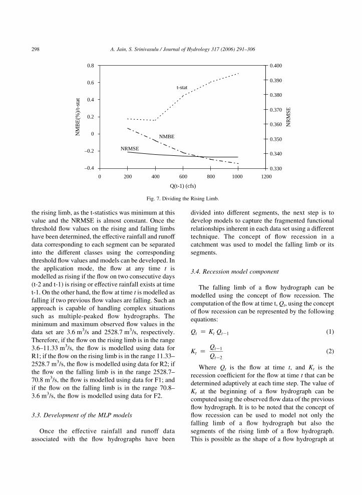
the flow hydrographs. Figs. 6 and 7 show the plots of

–3.50

–3.00

–2.50

–2.00

–1.50

–1.00

–0.50

0.00

0.50

1.00

1.50

2.00

0 2000 4000 6000 8000

Q(t-1) (c

NM

BE

(%)/

t-st

at

t-stat

NMBE

Fig. 6. Dividing the

these error statistics for different levels of the flow

value for dividing the falling limb and the rising limb,

respectively. It can be noted from the Fig. 6 that a flow

value of 70.8 m3/s (or 2500 ft3/s) is the most suitable

for dividing the falling limb as most of the error

curves converge to a minimum at this flow value.

Similarly, the Fig. 7 indicates that a flow value of

11.33 m3/s (400 ft3/s) is suitable to divide the data on

10000 12000 14000 16000

fs)

0.330

0.340

0.350

0.360

0.370

0.380

0.390

0.400

NR

MSENRMSE

Falling Limb.

–0.4

–0.2

0

0.2

0.4

0.6

0.8

0 200 400 600 800 1000 1200

Q(t-1) (cfs)

NM

BE

(%)/

t-st

at

0.330

0.340

0.350

0.360

0.370

0.380

0.390

0.400

NR

MSE

t-stat

NMBE

NRMSE

Fig. 7. Dividing the Rising Limb.


the rising limb, as the t-statistics was minimum at this

value and the NRMSE is almost constant. Once the

threshold flow values on the rising and falling limbs

have been determined, the effective rainfall and runoff

data corresponding to each segment can be separated

into the different classes using the corresponding

threshold flow values and models can be developed. In

the application mode, the flow at any time t is

modelled as rising if the flow on two consecutive days

(t-2 and t-1) is rising or effective rainfall exists at time

t-1. On the other hand, the flow at time t is modelled as

falling if two previous flow values are falling. Such an

approach is capable of handling complex situations

such as multiple-peaked flow hydrographs. The

minimum and maximum observed flow values in the

data set are 3.6 m3/s and 2528.7 m3/s, respectively.

Therefore, if the flow on the rising limb is in the range

3.6–11.33 m3/s, the flow is modelled using data for

R1; if the flow on the rising limb is in the range 11.33–

2528.7 m3/s, the flow is modelled using data for R2; if

the flow on the falling limb is in the range 2528.7–

70.8 m3/s, the flow is modelled using data for F1; and

if the flow on the falling limb is in the range 70.8–

3.6 m3/s, the flow is modelled using data for F2.

3.3. Development of the MLP models

Once the effective rainfall and runoff data

associated with the flow hydrographs have been

divided into different segments, the next step is to

develop models to capture the fragmented functional

relationships inherent in each data set using a different

technique. The concept of flow recession in a

catchment was used to model the falling limb or its

segments.

3.4. Recession model component

The falling limb of a flow hydrograph can be

modelled using the concept of flow recession. The

computation of the flow at time t, Qt, using the concept

of flow recession can be represented by the following

equations:

Qt Z Kt QtK1 (1)

Kt ZQtK1

QtK2

(2)

Where Qt is the flow at time t, and Kt is the

recession coefficient for the flow at time t that can be

determined adaptively at each time step. The value of

Kt at the beginning of a flow hydrograph can be

computed using the observed flow data of the previous

flow hydrograph. It is to be noted that the concept of

flow recession can be used to model not only the

falling limb of a flow hydrograph but also the

segments of the rising limb of a flow hydrograph.

This is possible as the shape of a flow hydrograph at


the beginning of the rising limb (R1) can be assumed

to be close to the mirror image of the flow hydrograph

at the final segment of the falling limb (F3).

3.5. ANN model component

A feed-forward multi-layer perceptron (MLP) type

ANN with the ‘generalized delta rule’ (Rumelhart

et al., 1986) as the training algorithm was employed

for the development of all the five MLP models. While

developing an MLP model, the primary objective is to

arrive at the optimum architecture to capture the

relationship among the various input and output

variables. All the MLP models developed in this

study consisted of three layers; an input layer, a hidden

layer, and an output layer. The task of identifying the

number of neurons in the input and output layers is

simple as it is dictated by the input and output

variables involved in the problem. In this study,

the neurons in the input layer represented Pt, Pt-1, Pt-2,

Qt-1, and Qt-2, while the only neuron in the output layer

represented Qt. The rainfall and runoff data were

scaled in the range of 0 and 1 using a linear

transformation in this study. The number of neurons

in the hidden layer (N) is determined using a trial and

error procedure by varying N in the range of 1 to 20

and examining a wide variety of statistical measures

during training for each N to select the best value of N.

The final architecture of the MLP model can be

selected based on the performance of each MLP in

terms of certain error statistics (described later). The

value of a learning coefficient of 0.01 and a

momentum correction factor of 0.075, and the

unipolar sigmoid activation function was used to

train all the MLP models. The problem of over-

parameterisation and ensuring against under-training/

over-training was handled by using a wider variety of

error statistics (described later) during training of the

ANN models. Once the training of the MLP models

was completed, they were validated using the testing

data set that they had not seen before.

3.6. The SOM models

In order to test the proposed methodology of

decomposing a flow hydrograph based on physical

concepts and develop different models for the

different segments, another type of ANN models

called the self-organizing map (SOM) models, were

developed. In this study, a one-dimensional Koho-

nen’s SOM model that employs an unsupervised

training algorithm to decompose the effective rainfall

runoff data into the different classes, was used. A

training method similar to the one adopted by

Abrahart and See (2000) was used to train the SOM

models developed in this study. The SOM training

starts by initializing the weight vector and normal-

isation of input vectors. The winning neuron was

selected based on competitive learning and similarity

clustering. The similarity rule of Euclidian distance is

the most popular method and was used in this study.

The weights of the winner neuron and its neighbours

were updated using Kohonen’s rule. The procedure

was repeated by presenting all input vectors and

convergence was achieved by fine tuning the learning

rate and the size of the neighbourhood. The values of

learning rate and neighbourhood distance of 0.9 and

0.2 were finally employed in this study to achieve

convergence in ordering and tuning phases. Two

different SOM models were developed: the first one,

called the SOM(3) model, explored the possibility of

three classes of the rainfall runoff mappings, and the

second one, called the SOM(4) model, explored for

the possibility of four classes of the rainfall runoff

mappings in the input output space. Once the input

output space was divided into the different classes

using a SOM classifier, the data from each class were

used to develop separate MLP models using the

supervised training method discussed earlier. The

optimum architecture of each MLP model based on

SOM, the number of patterns used to train, descriptive

statistics (mean and standard deviation) and the

associated input variables are presented in Table 1.

It may be noted that the SOM classifications

correspond to different magnitude flows e.g. low,

medium, and high based on the descriptive statistic in

terms of mean.

4. Study area and data

The data derived from the Kentucky River

catchment were employed to train and test all the

models developed in this study. The Kentucky River

catchment, shown in Fig. 8, encompasses over 4.4

million acres (17,820 km2) of the state of Kentucky.

Fig. 8. Kentucky River Catchment.


Forty separate counties lie either completely or

partially within the boundaries of the catchment.

The Kentucky River is the sole source for the several

water supply companies of the state. There is a series

of fourteen Locks and Dams on the Kentucky River,

which are owned and operated by the US Army Corps

of Engineers. The drainage area of the Kentucky

River at Lock and Dam 10 (LD10) near Winchester,

Kentucky is approximately 10,240 km2 and the time

of concentration of the catchment is approximately

two days. The data used in this study include the

average daily streamflow (m3/s) from Kentucky River

at LD10, and the daily average rainfall (mm) from the

five rain gauges (Manchester, Hyden, Jackson,

Heidelberg, and Lexington Airport) scattered

throughout the Kentucky River catchment (see the

Fig. 8). A total length of the data of 26-years (1960–

1989 with data in some years missing) was available.

The data were divided into two sets: a training data set

consisting of the daily rainfall and flow data for


thirteen years (1960–1972), and a testing data set

consisting of the daily rainfall and flow data of

thirteen years (1977–1989).

5. Model performance

The performance of all the models developed in

this study was evaluated using seven different

standard statistical measures. These are average

absolute relative error (AARE), threshold statistic

(TS), Pearson coefficient of correlation (R), Nash-

Sutcliffe efficiency (E), normalized mean bias error

(NMBE), normalized root mean square error

(NRMSE), and coefficient of persistence (Eper). All

of these statistics are unbiased in nature as they use

the error statistic relative to the observed values in

some form or the other. The TS and AARE statistics

have been used by the authors extensively in the past

(Jain et al., 2001; Jain and Ormsbee, 2002; Jain and

Indurthy, 2003; and Jain and Ormsbee, 2004). The

NMBE statistic indicates an over-estimation or under-

estimation in the estimated values of the physical

variables being modelled, and provides the infor-

mation on the long-term performance. The NRMSE

statistics provides the information for short-term

performance of a model by allowing a term by term

comparison of the actual differences between the

estimated and observed values. The Eper statistic is

used to evaluate the quality of a model in comparison

of a persistence model. The equations to compute the

AARE, TS, NMBE, NRMSE, and Eper statistics only

are provided here and the equations of calculating the

R and E statistics can be found in a standard text.

AARE Z1

N

XN

tZ1

QOðtÞKQPðtÞ

QOðtÞ

��X 100% (3)

TSx Znx

N!100% (4)

NMBE Z1N

PNtZ1ðQPðtÞKQOðtÞÞ1N

PNtZ1 QOðtÞ

X 100% (5)

NRMSE Z1N

PNtZ1ðQPðtÞKQOðtÞÞ2

� �1=2

1N

PNtZ1 QOðtÞ

(6)

Eper Z 1 K

PNtZ1ðQPðtÞKQOðtÞÞ2PN

tZ1ðQOðtÞKQOðt K1ÞÞ2(7)

Where QO(t) is the observed flow at time t, QO(t-1)

is the observed flow at time t-1, QP(t) is the predicted

flow at time t, nx is the total number of flow data points

predicted in which the absolute relative error (ARE) is

less than x%, and N is the total number of flow data

points predicted. The threshold statistic for the ARE

levels of 1, 5, 25, 50, and 100% were computed in

this study.

The TS and AARE statistics measure the ‘effec-

tiveness’ of a model in terms of its ability to

accurately predict flow from a calibrated model. The

other statistics, R, E, NMBE, and NRMSE, quantify

the ‘efficiency’ of a model in capturing the extremely

complex, dynamic, non-linear, and fragmented rain-

fall-runoff relationships. A model that is ‘effective’ in

accurately predicting the flow, and ‘robust’ or

‘efficient’ in capturing the complex relationship

among the various input and output variables involved

in a particular problem, is considered the best.

6. Results and discussions

The results in terms of the various statistical

measures during training and testing are presented in

Tables 2 and 3, respectively. It can be noticed from

the Table 2 that the performance of various models

during training becomes better as we move down the

table from the Model-I to the Model-V. Among the

MLP models, the best values of the AARE, R, E,

NMBE, NRMSE, and Eper statistics of 23.85%,

0.9780, 0.9570, K0.08, 0.338, and 0.743, respect-

ively, were obtained from the Model-V. Also, more

than 95% of the predicted flow values from the

Model-V had ARE less than 100% (see TS100 in

Table 2). These results show that the Model-V was the

best MLP model during training. Further, the

performance of both the SOM models is marginally

better than the Model-V in terms of the AARE, some

TS, R, E, NRMSE, Eper statistics but is worse in terms

of the NMBE and other TS statistics. Thus, the

performance of both the Model-V and SOM models is

comparable during training. Further, within the SOM

models, the SOM(4) model performed better than the

SOM(3) model indicating that the rainfall runoff data

Table 2

Performance evaluation statistics during training

Model TS1 TS5 TS25 TS50 TS100 AARE R E NMBE(%) NRMSE Eper

MLP Models

Model-I 3.20 14.17 51.67 69.37 82.19 54.97 0.9770 0.9545 1.68 0.347 0.736

Model-II 2.63 12.92 50.29 67.45 80.17 61.28 0.9764 0.9531 1.87 0.353 0.722

Model-III 6.76 27.79 72.19 85.00 92.65 31.66 0.9607 0.9215 K1.75 0.456 0.536

Model-IV 6.11 25.20 71.87 85.55 92.60 31.90 0.9777 0.9560 0.10 0.342 0.740

Model-V 6.25 26.70 74.71 88.55 95.40 23.85 0.9780 0.9570 K0.08 0.338 0.743

SOM Models

SOM(3) 4.63 21.36 70.00 88.39 97.85 23.22 0.9793 0.9591 0.21 0.328 0.759

SOM(4) 4.27 22.06 72.27 90.89 98.44 20.80 0.9804 0.9612 0.12 0.320 0.772


from the Kentucky River catchment possibly consist

of four classes corresponding to the different

dynamics. This finding is in line with dividing a

flow hydrograph into four segments corresponding to

the different dynamics while developing the inte-

grated ANN rainfall runoff models.

Observing the performance of various models

during testing also showed a similar trend. The

Model-V performed better than the remaining models

in terms of the effectiveness in predicting flow values

accurately as can be seen from the TS and AARE

statistics in the Table 3. For example, the best AARE

value of 21.63% was obtained from the Model-V, and

in 97.62% of the predicted cases from the Model-V,

ARE values were less than 100%. Although the

Model-I was marginally better in terms of the R, E,

NRMSE, and Eper statistics, and the Model-II was

better in terms of the NMBE statistics during testing,

their capability in effectively predicting the flow

accurately was extremely poor (see the TS and AARE

statistics in the Table 3). The efficiency of the Model-

V in modelling a rainfall-runoff process in terms of

the R, E, NRMSE, and Eper statistics was comparable

Table 3

Performance evaluation statistics during testing

Model TS1 TS5 TS25 TS50 TS100 A

MLP Models

Model-I 2.94 14.51 54.93 69.80 80.15 65

Model-II 2.85 12.98 52.96 68.98 79.22 72

Model-III 7.73 31.23 73.02 85.48 92.16 36

Model-IV 6.47 25.67 67.29 83.44 91.80 39

Model-V 7.01 28.07 72.34 89.62 97.62 21

SOM Models

SOM(3) 4.29 20.75 63.06 83.43 94.81 28

SOM(4) 2.59 13.73 61.75 86.17 97.61 26

to the other models. It is apparent that the SOM

models do not perform as well during testing as they

did during training. Among themselves, the SOM(4)

model performed better than the SOM(3) model in

terms of some TS and AARE statistics, and

comparable in terms of the others.

A model that is both ‘efficient’ in modelling and

‘effective’ in predicting accurately is preferred over a

model that is the most efficient in modelling and not

very effective in predicting flow accurately. There

seems to be a trade off among the two different

capabilities of a model, therefore, the final model

structure needs to be selected based on the optimum

trade off desired depending on the application of the

model. For example, a daily flow forecasting model is

suitable for the operational purposes for managing the

various water resources projects, therefore, a model

with good ‘efficiency’ in modelling and very good

‘effectiveness’ in predicting flow accurately is

desirable. Considering these issues, the Model-V is

deemed to be the best model for forecasting daily flow

in the Kentucky River catchment. The performance of

the Model-V during testing in the graphical form in

ARE R E NMBE (%) NRMSE Eper

.71 0.9700 0.9406 K0.19 0.389 0.689

.28 0.9696 0.9398 K0.02 0.393 0.681

.45 0.9571 0.9150 K2.44 0.466 0.549

.56 0.9684 0.9376 2.22 0.398 0.674

.63 0.9678 0.9366 0.65 0.402 0.684

.59 0.9680 0.9367 K2.24 0.401 0.665

.51 0.9620 0.9100 9.63 0.478 0.523

0

500

1000

1500

2000

2500

3000

0 500 1000 1500 2000 2500 3000

Observed flow (m3/sec)

Pred

icte

d fl

ow (

m3 /

sec)

Fig. 9. Scatter Plot of Observed and Predicted Flow from Model -V.


terms of the observed and predicted flows as a scatter

plot is shown in the Fig. 9, and the observed and

predicted flow for a sample year (1988) is shown in

the Fig. 10. These figures confirm that the Model-V is

able to predict the flow values very accurately. It is

worth mentioning that the Model-V is able to predict

the flow accurately for all magnitudes (e.g. low,

medium, and high) as indicated by the uniform spread

around the ideal line in Fig. 9.

Further, comparing the performances of the

Model-II and the Model-III, it was found that

modelling the falling limb using the concept of flow

0

500

1000

1500

0 50 100 150

Tim

Flow

(m

3 /se

c)

Fig. 10. Observed and Predicted Fl

recession is a better approach than modelling the

falling limb using an ANN technique in terms of the

effectiveness in prediction but not necessarily in terms

of the efficiency in modelling. That is, an ANN

technique is good in the efficient modelling while a

conceptual technique of flow recession is good in

predicting the flow values more accurately. Therefore,

an approach that is based on a combination of these

two techniques for modelling the falling limb may

yield a better model performance. This is verified by

comparing the results obtained from the Model-III

and the Model-IV that are same of the rising limb but

differ in the manner of modelling the falling limb. The

model that decomposed the falling limb into two

segments, and modelled initial segment dominated by

the surface flow and interflow using an ANN

technique and the latter segment dominated by the

base flow using a deterministic technique (the Model-

IV) was able to achieve good ‘efficiency’ in modelling

(advantage of the Model-II) and good ‘effectiveness’

in prediction (advantage of the Model-III). Therefore,

decomposing the falling limb of a flow hydrograph

into two segments and employing an integrated

approach of using the different techniques to model

the different segments is a better approach than using

a single technique to model the whole falling limb.

Further, comparing the performance of the Model-IV

and the Model-V, which are same on the falling limb

but differ in the manner of modelling the rising limb, it

200 250 300 350

e in days

Observed flow

Predicted flow

ow from Model-V for 1988.


can be noted that the Model-V performs better than

the Model-IV in terms of most of the statistics during

both the training and the testing data sets. This

suggests that decomposing the rising limb into two

segments and employing an integrated approach to

model the initial segment of the rising limb (R1),

which is dominated by the infiltration capacities, drier

soil moisture and catchment storage conditions, using

a conceptual technique, and latter segment of the

rising limb (R2) characterized by the soil moisture and

catchment storage conditions close to saturation using

an ANN technique, is a better approach than using a

single technique to model the whole rising limb of a

flow hydrograph.

The ANNs are powerful tools of modelling and

forecasting the non-linear systems such as a flow

hydrograph. Therefore, an integrated approach of

using the ANN and conceptual techniques coupled

with the decomposition of a larger problem into the

smaller simpler ones can be quite ‘effective and

efficient’ and needs to be explored further. However,

one question which arises is that why an integrated

approach coupled with a decomposition method is

able to perform better than the approach using a single

technique or modelling the whole hydrograph. One

possible reason may be that, mathematically, approxi-

mating one complex function in place of the two or

more simpler functions of varying natures (due to the

different physical processes responsible for them)

gives a numerically averaged result, and can be biased

towards one type of function. Thus, approximating the

two or more different rainfall runoff relationships (e.g.

the high, medium, and low magnitude flows corre-

sponding to the different dynamics) using a single

function approximator (an ANN) may, in fact, cause

high errors in estimating either the high magnitude

flows, the medium magnitude flows, or the low

magnitude flows. Hsu et al. (1995) found that the

ANN models under-predicted the low flows and over-

predicted the medium flows. Sajikumar and Thanda-

veswara (1999); and Tokar and Markus (2000)

recently reported that the ANN models they

developed were not able to learn the rainfall-runoff

relationships properly for the low flows having the

target values close to zero. This has also been the

experience of the authors in using the ANNs for

rainfall runoff modelling (Jain and Srinivasulu, 2004).

In light of such findings, the integrated approach

proposed in this study can be extremely useful in

developing efficient models of the complex, dynamic,

and non-linear rainfall-runoff process that are also

quite effective in accurately predicting flow hydro-

graphs from a catchment.

7. Summary and conclusions

This paper presents the findings of a study aimed at

developing an integrated approach for the flow

hydrograph modelling by embedding the components

of a hydrologic process modelled using the conceptual

technique in an artificial neural network (ANN)

model, and modelling the decomposed flow hydro-

graph using a combination of the ANN and conceptual

techniques. The genesis of the study presented in this

paper is based on the concept that the different

segments of a flow hydrograph are the results of the

different physical processes in a catchment and need

the different techniques for modelling. In this study,

five MLP type and two SOM type ANN rainfall runoff

models were developed. All the ANN models

employed the effective rainfall computed using the

conceptual techniques and the past flow values as the

input variables. The rainfall and streamflow data

derived from the Kentucky River catchment were

employed to test the proposed methodology and

develop all the models investigated in this study.

Seven different standard statistical measures were

employed to evaluate the performance of each model

structure investigated in this study. The following

conclusions can be drawn from this study:

1. An integrated modelling framework capable of

exploiting the strengths of the ANN and concep-

tual techniques to model different segments of a

decomposed flow hydrograph can be a better

alternative than adopting either a purely concep-

tual or a purely black box approach for the

hydrologic modelling in terms of both ‘efficiency’

in modelling and ‘effectiveness’ in accurately

predicting flows.

2. The results obtained in this study indicate that the

rainfall runoff relationships in a large catchment

may consist of three or four different mappings

corresponding to the different dynamics of the

underlying physical processes.


3. Modelling the falling limb of a flow hydrograph

using the concept of flow recession is a better

approach than using an ANN in predicting the flow

values accurately.

4. Decomposing the rising limb or the falling limb of

the flow hydrograph into two segments and

employing an integrated approach of using the

different techniques to model different segments is

a better approach than using a single technique to

model the whole rising limb or the whole falling

limb.

5. The superiority of the Model-V over the SOM

models indicates that dividing the rainfall runoff

data space into the different classes corresponding

to the different dynamics based on the physical

concepts is better than relying on the self

organizing neural networks for classification.

6. The methodology proposed in this study is able to

capture the different dynamics inherent in the low,

medium, and high magnitude flows using the

decomposing techniques to overcome some of the

problems of under-and over-prediction of certain

magnitude flows reported by others (Hsu et al.,

1995; Sajikumar and Thandaveswara, 1999; Tokar

and Markus, 2000; and Jain and Srinivasulu, 2004)

The authors believe that no study is complete in

itself and there is always a scope for improvements.

The study presented in this paper developed the

conceptual components of the hydrologic process and

the ANN rainfall runoff models using spatially

aggregated rainfall taken from five different rain-

gauges scattered throughout a large catchment. The

spatial averaging of the distributed rainfall tends to

dampen the dynamic effects inherent in the rainfall-

runoff relationship that is distributed in nature. Ideally,

a distributed hydrologic model and an ANN rainfall

runoff model that employs the individual rainfalls from

the different raingauges scattered throughout a large

catchment need to be developed to have more

confidence in the findings of such studies. However,

a distributed approach to hydrologic modelling would

significantly complicate the solution procedures.

Another issue that needs to be explored further is the

manner of decomposing a flow hydrograph. This was

achieved by using physical concepts to decompose the

rising and falling limbs of a flow hydrograph into two

segments each using a trial and error method to

minimize errors in predicting the flow hydrographs.

One can analyze different flow hydrographs of varying

magnitudes from a catchment more closely and deduce

certain patterns and rules based on physical concepts

that can be employed in decomposing a flow

hydrograph. Further, a possibility of achieving

improved model performance by dividing rising and

falling limbs of a flow hydrograph into further finer

segments and develop integrated models remains to be

explored. It is hoped that the future research efforts will

focus on the use of the proposed integrated techniques

for modelling decomposed flow hydrograph in other

catchments of varying hydrological and climatic

conditions to strengthen the findings of this study.

References

Abrahart, R.J., See, L., 2000. Comparing neural network and

autoregressive moving average techniques for the provision of

continuous river flow forecasts in two contrasting catchments.

Hydrol. Process. 14, 2157–2172.

Anctil, F., Tape, D.G., 2004. An exploration of artificial neural

network rainfall-runoff forecasting combined with wavelet

decomposition. J. Env. Eng. Sci. 3 (1), S121–S128.

Arnold, J.G., Allen, P.M., Muttiah, R., Bernhardt, G., 1995.

Automated base flow separation and recession analysis

techniques. Ground Water 33 (6), 1010–1018.

Birikundavyi, S., Labib, R., Trung, H.T., Rousselle, J., 2002.

Performance of neural networks in daily streamflow Forecast-

ing. J. Hydrol. Eng., ASCE 7 (5), 392–398.

Bishop, C.M., 1995. Neural Networks for Pattern Recognition.

Clarendon Press, Oxford, UK.

Campolo, M., Andreussi, P., Soldati, A., 1999. River flood

forecasting with neural network model. Water Resour. Res. 35

(4), 1191–1197.

Chakraborty, K., Mehrotra, K., Mohan, C.K., Ranka, S., 1992.

Forecasting the behaviour of the multivariate time series using

neural networks. Neural Networks 5, 961–970.

Dawson,D.W.,Wilby,R.,1998.Anartificialneuralnetworkapproach

to rainfall-runoff modeling. Hydrol. Sci. J. 43 (1), 47–65.

Furundzic, D., 1998. Application example of neural networks for

time series analysis: rainfall runoff modeling. Signal Process.

64, 383–396.

Haan, C.T., 1972. A water yield model for small watersheds. Water

Resour. Res. 8 (1), 58–69.

Hsu, K.L., Gupta, H.V., Sorooshian, S., 1995. Artificial neural

network modeling of the rainfall-runoff process. Wat. Resour.

Res. 31 (10), 2517–2530.

Hsu, K.L., Gupta, H.V., Gao, X., Sorooshian, S., Imam, B., 2002.

Self-organizing linear output map (SOLO): an artificial neural

network suitable for hydrologic modeling and analysis. Water

Resour. Res. 38 (12), 1302 (doi:10.1029/2001WR000795).


Jain, A., Ormsbee, L.E., 2002. Evaluation of short-term water

demand forecast modeling techniques: conventional methods

versus AI. J. Am. Water Works Assoc. 94 (7), 64–72.

Jain, A., Indurthy, S.K.V.P., 2003. Comparative analysis of event

based rainfall-runoff modeling techniques-deterministic, stat-

istical, and artificial neural networks’. J. Hydrol. Engg., ASCE 8

(2), 1–6.

Jain, A., Ormsbee, L.E., 2004. An evaluation of the available

techniques for estimating missing fecal coliform data. J. Am.

Water Resour. Assoc. 40 (6), 1617–1630.

Jain, A., Srinivasulu, S., 2004. Development of effective and

efficient rainfall-runoff models using integration of determinis-

tic, real-coded GA, and ANN techniques. Water Resour. Res. 40

(4) (W04302, doi:10.1029/2003WR002355).

Jain, A., Varshney, A.K., Joshi, U.C., 2001. Short-term water

demand forecast modeling at IIT Kanpur using artificial neural

networks. Water Resour. Manage. 15 (5), 299–321.

Jain, A., Sudheer, K.P., Srinivasulu, S., 2004. Identification of

physical processes inherent in artificial neural network rainfall

runoff models? Hydrol. Process. 118 (3), 571–581.

Kumar, A., Minocha, K., 2001. Discussion on rainfall runoff

modeling using artificial neural networks. J. Hydrol. Eng.,

ASCE 6 (2), 176–177.

Labat, D., Ababou, R., Mangin, A., 2000. Rainfall-runoff relations

for Karstic springs. Part II: continuous wavelet and discrete

orthogonal multiresolution. J. Hydrol. 238 (3–4), 149–178.

Labat, D., Ababou, R., Mangin, A., 2001. Introduction of wavelet

analyses to rainfall-runoff relationship for a Karstic basin: The

case of Licq-Atherey Karstic system, France. Ground Water 39

(4), 605–615.

Liu, S.Y., Quan, X.Z., Zhang, Y.C., 2003. Application of wavelet

transform in runoff sequence analysis. Progr. Nat. Sci. 13 (7),

546–549.

Minns, A.W., Hall, M.J., 1996. Artificial neural networks as rainfall

runoff models. Hydrol. Sci. J. 41 (3), 399–417.

Rumelhart, D.E., Hinton, G.E., Williams, R.J., 1986. Learning

representations by back-propagating errors. Nature 323,

533–536.

Sajikumar, N., Thandaveswara, B.S., 1999. A non-linear rainfall-

runoff model using an artificial neural network. J. Hydrol. 216,

32–55.

Shamseldin, A.Y., 1997. Application of a neural network technique

to rainfall-runoff modeling. J. Hydrol. 199, 272–294.

Smith, J., Eli, R.N., 1995. Neural network models of the rainfall

runoff process. ASCE J. Res. Plan. Manage. 121, 499–508.

Smith, L.C., Turcotte, D.L., Isacks, B.L., 1998. Streamflow

characterization and feature detection using a discrete wavelet

transform. Hydrol. Process. 12 (2), 233–249.

Spongberg, M.E., 2000. Spectral analysis of base flow separation

with digital filters. Water Resour. Res. 36 (3), 745–752.

Sudheer, K.P., Jain, A., 2004. Explaining the internal behavior of

artificial neural network river flow models. Hydrol. Process. 118

(4), 833–844.

Tokar, A.S., Markus, M., 2000. Precipitation runoff modeling using

artificial neural network and conceptual models. J. Hydrol. Eng.,

ASCE 5 (2), 156–161.

Wilby, R.L., Abrahart, R.J., Dawson, C.W., 2003. Detection of

conceptual model rainfall-runoff processes inside an artificial

neural network. Hydrol. Sci. J. 48 (2), 163–181.

Zhang, B., Govindaraju, S., 2000. Prediction of Watershed Runoff

using Bayesian Concepts and Modular Neural Networks. Water

Resour. Res. 36 (3), 753–762.

Zhu, ML, Fujita, M, Hashimoto, N, 1994. Application of neural

networks to runoff prediction. In: Hippel, K.W. et al. (Ed.),

Stochastic and Statistical Methods in Hydrology and Environ-

mental Engineering. Kluwer Academic, Norwell, MA, pp. 205–

216.

Zurada, M.J., 1997. An Introduction to Artificial Neural Systems.

Jaico Publishing House, Mumbai, India, in arrangement with

West Publishing Company, St Paul, Minnesota.

Documents

Integrated approach to model decomposed flow hydrograph using artificial neural network and conceptual techniques