Embed Size (px)
Citation preview

Instrumental Variables I
IVs are not magic
1. Review: Problems that extra variables and experiments don’t solve. 1a. Discussing omitted variable bias in VSPs
2. IV vs. Measurement Error
3. IV vs. Selection Bias: Selection in Military Service & Draft Lottery – Angrist (1990)
4. Wald Estimator
5. IV and Overidentification

1. Review: Pop. Parameters - What did
your sample regression aspire to estimate?
Sample Population
1. CEF
y = Xb + e, x’e=0 2. BLP
3. Causal Effect
4. Linear Causal Effect
5. Perfectly specified equation model including all relevant variables
In principle #4 and #5 yield identical population parameters for β1
if Cov (x1, ε | β2’x2) = 0, i.e., no omitted variable bias.

1. Review: Problems that extra
variables and experiments don’t solve. Solution
Problem
Add the omitted
var.
experiment instrument
1. Forgot X2
2. Selection
3. Meas. Err.
4. Misspecification
5. Heterogeneity
6. Endogeneity/
Simultaneity
Good omitted variables, experimental data and instruments are all hard to find.
Where do control functions and matching fit?

1a. Discussing omitted variable bias in VSP e.g. selection bias & reconstruction spending (CERP, JPE 2011)
-30
36
Vio
lence
-100 -50 0 50 100CERP
coef = .015, (robust) se = .004, t = 3.9
CERP w/controls
-30
36
Vio
lence
-100 -50 0 50 100CERP
coef = -.009, (robust) se = .004, t = -2.2
CERP in FD, 2004-08
-30
36
Vio
lence
-100 -50 0 50 100CERP
coef = -.018, (robust) se = .006, t = -3.0
CERP in FD, 2007-08

Discussing omitted variable bias:
reporting results ------ 2004-2008 ------
Incidents per
1000 (1) (2) (3) (4) (5) (6)
Basic controls Y Y
Time controls Y Y Y Y
First
differences Y Y Y
Pre-existing
trend (∆vt-1) Y Y
District specific
trends Y
CERP per
Capita
0.0213*** 0.0147*** 0.0115*** -0.00945** -0.0111** -0.0110**
(0.004) (0.0038) (0.0040) (0.0043) (0.0043) (0.0046)
Pre-existing
trend (∆vt-1)
0.195** 0.192**
(0.080) (0.087)
Constant 0.361*** 0.306** 0.262** 0.217*** -0.124*** 0.0890**
(0.085) (0.13) (0.10) (0.046) (0.041) (0.042)
Observations 1040 1000 1000 936 832 832
R-squared 0.08 0.25 0.33 0.17 0.21 0.21
MSPE (10-fold
CV) 3.52 3.05 2.81 4.77 4.95 5.25
TABLE 4
Violent Incidents
on CERP
Spending
(Berman,
Shapiro, Felter
JPE, August
2011)
Robust standard errors in parentheses, clustered by district. Results are robust to clustering by governorate instead. Regressions weighted by estimated population. Basic
controls include sect, unemployment, and income variables (as in Table 3). Time controls include year indicators and their interaction with Sunni vote share (as in Table 3).
District specific trends are district effects in a differenced specification. Basic controls are dropped from first-differenced specifications as they do not vary on a semi-
annual basis. *** significant at 1% level; ** significant at 5% level; * significant at 10% level
The limits of adding more variables and of
experiments
Adding the extra variables is expensive or
impossible
Experiments are often expensive, unethical
or impossible
- even when possible they are a lot of work
(see McIntosh course)

2. Instrumental Variables vs.
Measurement Error yi = β0 + β1x*i + εi
x*i not observed. The best we can do is observe a noisy measure of x*..
xi = x*i + vi , Cov (v,x*)=0, Cov(ε,x*)=0, Cov(v, ε)=0 “classical” measurement error assumptions
Rewrite as an omitted variable.. yi = β0 + β1 (xi – v) + εi
= β0 + β1xi - β1v + εi , (L)
yi = β0 + β1 xi + ui (S), Cov(x,u) ≠ 0
..and use OVB formula to solve
b1s = b1
L + b21 b2L
2. IV. vs. Meas. Error: Solution
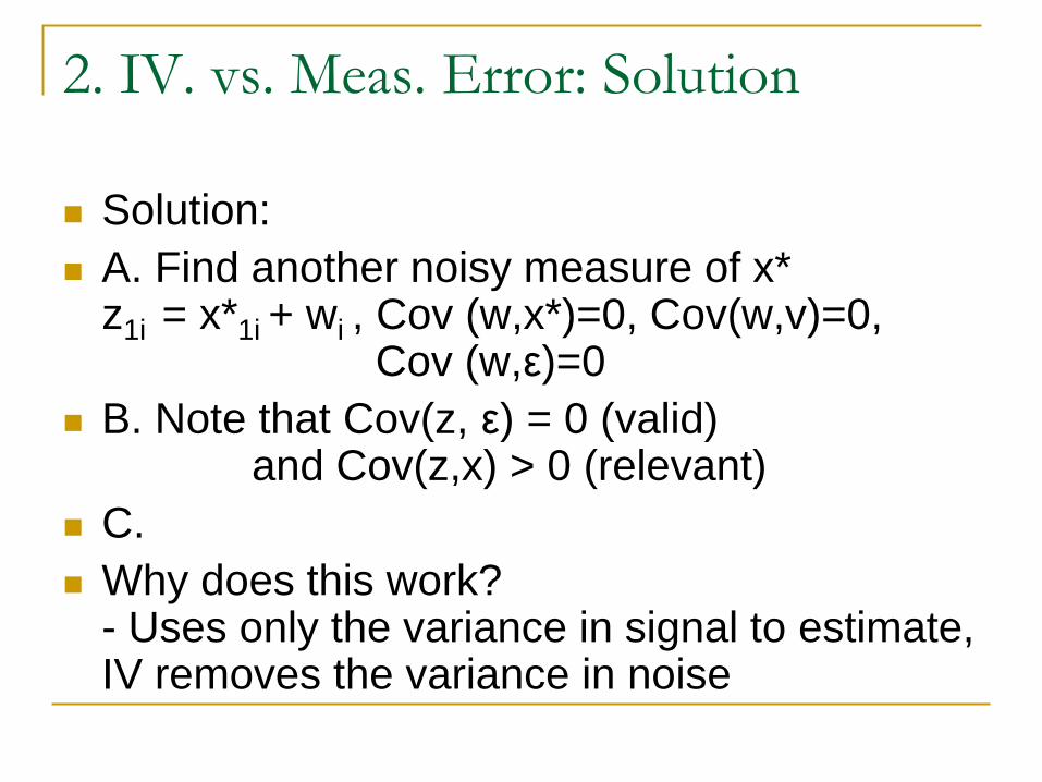
Solution:
A. Find another noisy measure of x* z1i = x*1i + wi , Cov (w,x*)=0, Cov(w,v)=0, Cov (w,ε)=0
B. Note that Cov(z, ε) = 0 (valid) and Cov(z,x) > 0 (relevant)
C.
Why does this work? - Uses only the variance in signal to estimate, IV removes the variance in noise

2. IV. Vs. Meas. Error – Returns to
Schooling in Twinsville Sample
Orley Ashenfelter and Alan Krueger set up a
booth at the annual Twinsville Twins festival
in 1991 and surveyed identical and fraternal
twins.
They were really looking for fixed-effects
estimates but they happened to ask the twins
to report each other’s schooling

2. IV. Vs. Meas. Error – Returns to
Schooling, Twinsville Data, AER 1994

2. IV. Vs. Meas. Error – Returns to
Schooling
Note: GLS is Seemingly Unrelated Regression (SUR)
3. IV vs. Selection Bias: Military Service
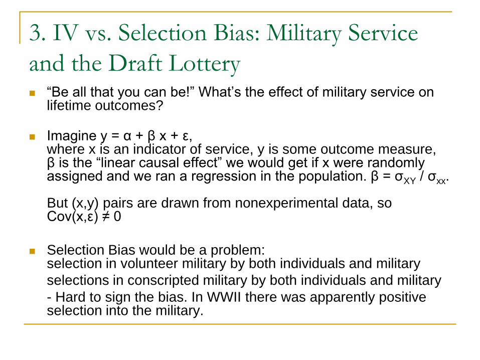
and the Draft Lottery “Be all that you can be!” What’s the effect of military service on
lifetime outcomes?
Imagine y = α + β x + ε, where x is an indicator of service, y is some outcome measure, β is the “linear causal effect” we would get if x were randomly assigned and we ran a regression in the population. β = ζXY / ζxx. But (x,y) pairs are drawn from nonexperimental data, so Cov(x,ε) ≠ 0
Selection Bias would be a problem: selection in volunteer military by both individuals and military
selections in conscripted military by both individuals and military
- Hard to sign the bias. In WWII there was apparently positive selection into the military.

3. IV vs. Selection Bias: Draft Lottery
Draft lottery over birthdates instituted in 1967
for 1950 birth cohort.
Someone pulled a ball with a birthdate on it
from a rotating bin with 365 balls, on national
TV.
z є (0,1) Cov(z, ε) = 0, Cov(z,x) > 0
Everyone with that birthdate was draft eligible
but not all eligibles ended up serving (e.g.,
Bill Clinton was z=1 but x=0.)

3. IV vs. Selection: Draft Lottery

Differences in Earnings w/ trend
removed [Reduced Form]

4. Wald Estimator
For a simple regression with a binary
instrument the IV estimator simplifies to a
Wald (1940) estimator.
IV estimator can also be interpreted as the
ratio of reduced form to first stage, in this
simple regression case.
Which variance (subpopulation) provides
identifying information?
(Forest Gump, Bill Clinton, groaners)

Effect of Eligibility on Service [1st Stage]
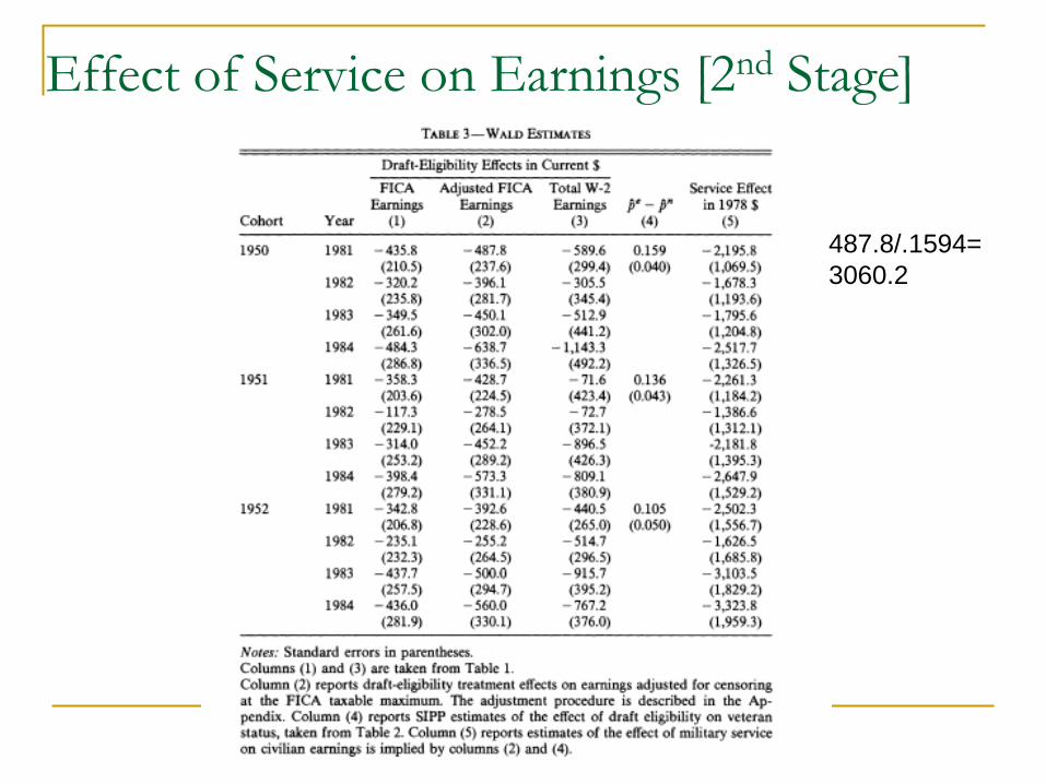
Effect of Service on Earnings [2nd Stage]
487.8/.1594=
3060.2

5. Efficient IV
estimates
and over-
identification
statistics
• Table 3 has multiple consistent
estimates, so
1) you can estimate more efficiently
by combining estimates, and
2) you can test a necessary condition
for validity.
OID interpretation and intuition

The Validity Oath
The only way that z can be correlated with y
is through its effect on x.
GI bill, generalizability
Draft avoidance behavior, Canada
What to do? OID tests

More clever IVs:

Next Time.. How we started worrying
about weak instruments and what to do
about it.
Angrist, Joshua and Alan B. Krueger (1991), "Does Compulsory School Attendance Affect Schooling?" Quarterly Journal of Economics, 106, 979-1014.
Bound, John, David Jaeger and Regina Baker, (1995) "Problems with Instrumental Variables Estimation when the Correlation Between the Instruments and the Endogenous Explanatory Variables is Weak," Journal of the American Statistical Association, 90 (June): 443-450.
Instrumental Variables II
Weak Instruments
1. Review: The attraction of IV
2. IV vs. Heterogeneity Bias: Compulsory Schooling, birth quarter and earnings – Angrist & Krueger (1991)
3. Weak instrument bias in two flavors
4. Protection against weak instrument bias
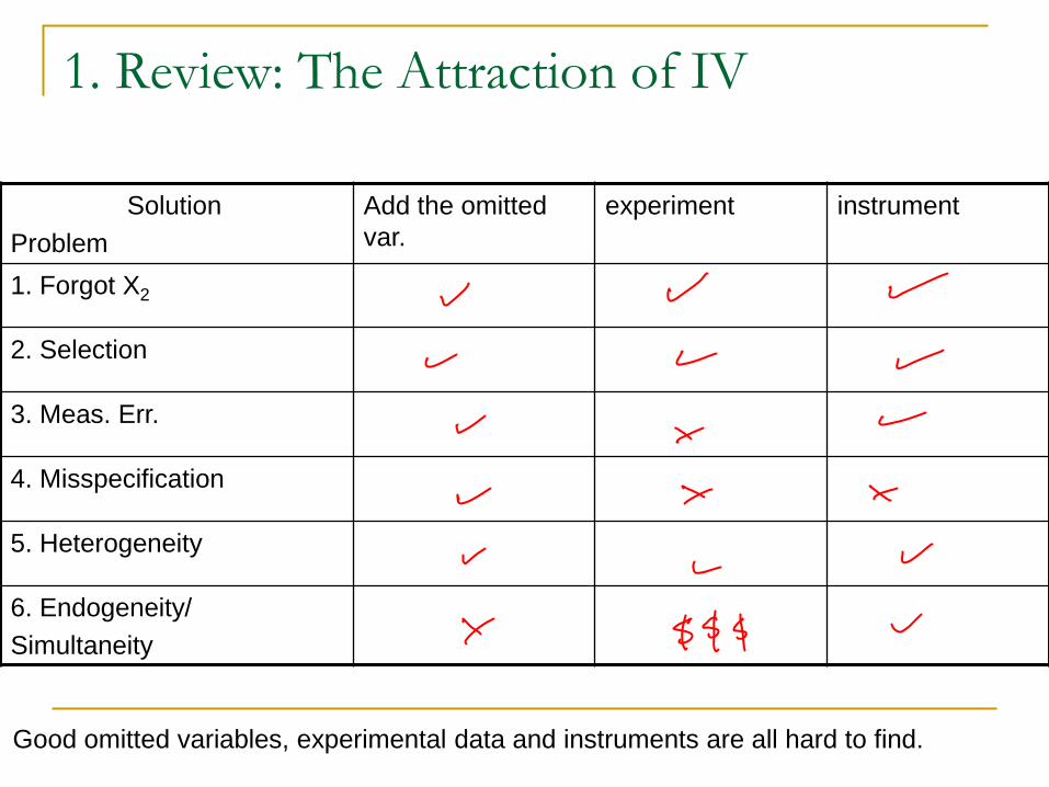
1. Review: The Attraction of IV
Solution
Problem
Add the omitted
var.
experiment instrument
1. Forgot X2
2. Selection
3. Meas. Err.
4. Misspecification
5. Heterogeneity
6. Endogeneity/
Simultaneity
Good omitted variables, experimental data and instruments are all hard to find.

1. Review: The attraction of IV
Sample Population
1. CEF
y = Xb + e, x’e=0 2. BLP
b ols 3. Causal Effect
4. Linear Causal Effect
5. Perfectly specified equation model including all relevant variables
bIV=(z’x)-1z’y has no interpretation as a predictor

2. IV vs. Heterogeneity Bias: Compulsory Schooling, birth
quarter and earnings – Angrist & Krueger (1991)
School boards have age at
entry requirements.
States have compulsory
schooling laws according to
age.
So a one-day difference in
birthdate can create a one
year difference in lifetime
schooling.

And it works..

Quarter of birth and schooling
completed

So here’s an instrument for ability in the
“Mincer” regression
yi = β0 + β1xi + X2 β2 + ai + εi
x1 – schooling, y – log(earnings)
The human capital wage regression (“Mincer” regression) is the foundation of human capital theory.
Yet we worry about bias due to unobserved ability, which is potentially correlated with schooling, Cov(x1,a)
z – quarter of birth, is a valid instrument if Cov(z, ε) = 0, i.e., quarter of birth affects earnings only through its’ effect on schooling. From Figure I we know that it’s relevant.

Reduced form: Do 1st quarter babies have
lower earnings (as adults)?

Wald Estimates

Two stage least squares

TSLS estimates:

Possible Validity Problems:
Why might quarter of birth be correlated with the residual in the earnings equation?
Age at entry and earnings
Season of birth and earnings
These seem like 2nd order problems,
OID tests don’t raise any red flags .. so we can stop worrying about ability bias in earnings equations and proudly claim that estimated returns to education are causal, right?

3. Weak instrument bias in IV estimators
The graduate labor class at the University of Michigan does replication exercises. (Moderately short papers).
Regina Baker and David Jaeger manage to replicate the results (Angrist and Krueger shared the data).
But two things bother them and Prof. Bound: (Tables 1 and 2).

Small Sample Bias of IV Estimators
Worry #1: The results are imprecise and unstable when the controls and instrument
sets change.

Small Sample Bias of IV Estimators
Worry #2:
The results become
precise and stable
only when the first
stage F tests cannot
reject coefficients
which are jointly
zero.
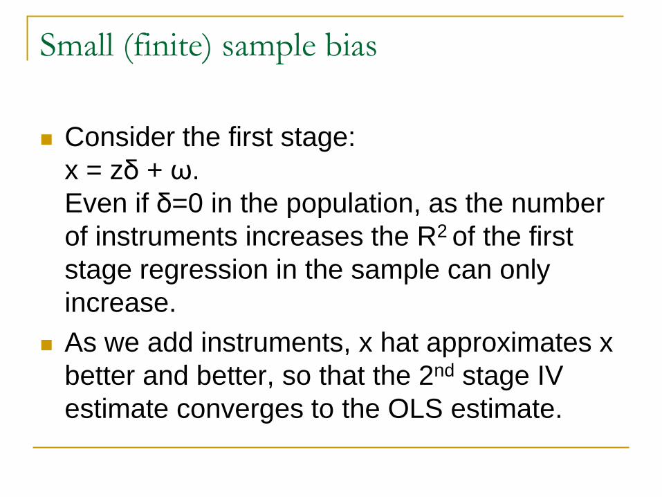
Small (finite) sample bias
Consider the first stage:
x = zδ + ω.
Even if δ=0 in the population, as the number
of instruments increases the R2 of the first
stage regression in the sample can only
increase.
As we add instruments, x hat approximates x
better and better, so that the 2nd stage IV
estimate converges to the OLS estimate.

Simulation with a random instrument
As an illustration, B,B and J
estimated the IV coefficient with
a randomly assigned Z so that
δ=0 by construction.
They did a great job reproducing
the OLS estimate.

Flavor #2:
Weak Instruments when the IV is almost,
but not quite, valid
• Is the cure worse than the disease?
• OLS bias vs. IV bias
• What looks like a second order Cov(z, ε) can create a
first order inconsistency if Cov(z,x) is small.

4. What to do about weak instruments?
First Stage F tests on the marginal excluded
instrument or sets of instruments
First Stage R2