Instrumental variable models for discrete outcomes · 2009-08-18 · Instrumental Variable Models for Discrete Outcomes 3 comparison with the single equation instrumental variable

Instrumental variable models for discrete outcomes Andrew Chesher

The Institute for Fiscal Studies Department of Economics, UCL cemmap working paper CWP30/08

Instrumental Variable Models for Discrete Outcomes

Andrew Chesher�

CeMMAP and UCL

Revised July 3rd 2009

Abstract. Single equation instrumental variable models for discrete out-comes are shown to be set not point identifying for the structural functions thatdeliver the values of the discrete outcome. Bounds on identi�ed sets are derivedfor a general nonparametric model and sharp set identi�cation is demonstratedin the binary outcome case. Point identi�cation is typically not achieved byimposing parametric restrictions. The extent of an identi�ed set varies withthe strength and support of instruments and typically shrinks as the support ofa discrete outcome grows. The paper extends the analysis of structural quan-tile functions with endogenous arguments to cases in which there are discreteoutcomes.

Keywords: Partial identi�cation, Nonparametric methods, Nonadditivemodels, Discrete distributions, Ordered choice, Endogeneity, Instrumental vari-ables, Structural quantile functions, Incomplete models.

JEL Codes: C10, C14, C50, C51.

1. Introduction

This paper gives results on the identifying power of single equation instrumentalvariables (IV) models for a discrete outcome, Y , in which explanatory variables, X,may be endogenous. Outcomes can be binary, for example indicating the occurrenceof an event; integer valued - for example recording counts of events; or ordered - forexample giving a point on an attitudinal scale or obtained by interval censoring ofan unobserved continuous outcome. Endogenous and other observed variables can becontinuous or discrete.

The scalar discrete outcome Y is determined by a structural function thus:

Y = h(X;U)

and it is identi�cation of the function h that is studied. Here X is a vector ofpossibly endogenous variables, U is a scalar continuously distributed unobservablerandom variable, normalised marginally uniformly distributed on the unit intervaland h is restricted to be weakly monotonic, normalised non-decreasing and càglàd inU .

There are instrumental variables, Z, excluded from the structural function h, andU is distributed independently of Z for Z lying in a set . X may be endogenousin the sense that U and X may not be independently distributed. This is a single

�Department of Economics, University College London, Gower Street, London WC1E 6BT, UK.Telephone: +442076795857. Email: [email protected].

1

Instrumental Variable Models for Discrete Outcomes 2

equation model in the sense that there is no speci�cation of structural equationsdetermining the value of X. In this respect the model is incomplete.

There could be parametric restrictions. For example the function h(X;U) couldbe speci�ed to be the structural function associated with a probit or a logit modelwith endogenous X, in the latter case:

h(X;U) = 1hU >

�1 + exp(X 0�)

��1iU � Unif(0; 1)

with U potentially jointly dependent with X but independent of instrumental vari-ables Z which are excluded from h. The results of this paper apply in this case. Untilnow instrumental variables analysis of binary outcome models has been con�ned tolinear probability models.

The central result of this paper is that the single equation IV model set identi�esthe structural function h. Parametric restrictions on the structural function do nottypically secure point identi�cation although they may reduce the extent of identi�edsets.

Underpinning the identi�cation results are the following inequalities:

for all � 2 (0; 1) and z 2 : Pra[Y � h(X; �)jZ = z] � �Pra[Y < h(X; �)jZ = z] < �

(1)

which hold for any structural function h which is an element of an admissible structurethat generates the probability measure indicated by Pra.

In the binary outcome case these inequalities sharply de�ne the identi�ed set ofstructural functions for the probability measure under consideration in the sense thatall functions h, and only functions h, that satisfy these inequalities for all � 2 (0; 1)and all z 2 are elements of the observationally equivalent admissible structureswhich generate the probability measure Pra.

When Y has more than two points of support the model places restrictions onstructural functions additional to those that come from (1) and the inequalities de�nean outer region1, that is a set within which lies the set of structural functions identi�edby the model. Calculation of the sharp identi�ed set seems infeasible when X iscontinuous or discrete with many points of support without additional restrictions.Similar issues arise in some of the models of oligopoly market entry discussed in Berryand Tamer (2006).

When the outcome Y is continuously distributed (in which case h is strictlymonotonic in U) both probabilities in (1) are equal to � and with additional com-pleteness restrictions, the model point identi�es the structural function as set out inChernozhukov and Hansen (2005) where the function h is called a structural quantilefunction. This paper extends the analysis of structural quantile functions to cases inwhich outcomes are discrete.

Many applied researchers facing a discrete outcome and endogenous explanatoryvariables use a control function approach. This is rooted in a more restrictive com-plete, triangular model which can be point identifying but the model�s restrictionsare not always applicable. There is a brief discussion in Section 4 and a detailed

1This terminology is borrowed from Beresteanu, Molchanov and Molinari (2008).


comparison with the single equation instrumental variable model in Chesher (2009).A few papers take a single equation IV approach to endogeneity in parametric

count data models, basing identi�cation on moment conditions.2 Mullahy (1997) andWindmeijer and Santos Silva (1997) consider models in which the conditional expec-tation of a count variable given explanatory variables, X = x, and an unobservedscalar heterogeneity term, V = v, is multiplicative: exp(x�) � v, with X and Vcorrelated and with V and instrumental variables Z having a degree of independentvariation. This IV model can point identify � but the �ne details of the functionalform restrictions are in�uential in securing point identi�cation and the approach,based as it is on a multiplicative heterogeneity speci�cation, is not applicable whendiscrete variables have bounded support.

The paper is organised as follows. The main results of the paper are given inSection 2 which speci�es an IV model for a discrete outcome and presents and dis-cusses the set identi�cation results. Section 3 presents two illustrative examples; onewith a binary outcome and a binary endogenous variable and the other involves aparametric ordered-probit-type problem. Section 4 discusses alternatives to the setidentifying single equation IV model and outlines some extensions including the casearising with panel data when there is a vector of discrete outcomes.

2. IV models and their identifying power

This Section presents the main results of the paper. Section 2.1 de�nes a singleequation instrumental variable model for a discrete outcome and develops the prob-ability inequalities which play a key role in de�ning the identi�ed set of structuralfunctions. In Section 2.2 theorems are presented which deliver bounds on the set ofstructural functions identi�ed by the IV model in theM > 2 outcome case and sharpidenti�cation in the binary outcome case. Section 2.3 discusses the identi�cationresults with brief comments on: the impact of support and strength of instrumentsand discreteness of outcome on the identi�ed set, sharpness, and local independencerestrictions.

2.1. Model. The following two restrictions de�ne a model, D, for a scalar discreteoutcome.

D1. Y = h(X;U) where U 2 (0; 1) is continuously distributed and h is weaklymonotonic (normalized càglàd, non-decreasing) in its last argument. X is avector of explanatory variables. The codomain of h is some ascending sequencefymgMm=1 which is independent of X. M may be unbounded. The function h isnormalised so that the marginal distribution of U is uniform.

D2. There exists a vector Z such that Pr[U � � jZ = z] = � for all � 2 (0; 1) andall z 2 .

A key implication of the weak monotonicity condition contained in RestrictionD1 is that the function h(x; u) is characterized by threshold functions fpm(x)gMm=0

2See the discussion in Section 11.3.2 of Cameron and Trivedi (1988).


as follows:

for m 2 f1; : : : ;Mg: h(x; u) = ym if and only if pm�1(x) < u � pm(x) (2)

with, for all x, p0(x) � 0 and pM (x) � 1. The structural function, h, is a non-decreasing step function, the value of Y increasing as U ascends through thresholdswhich depend on the value of the explanatory variables, X, but not on Z.

Restriction D2 requires that the conditional distribution of U given Z = z beinvariant with respect to z for variations within . If Z is a random variable and isits support then the model requires that U and Z be independently distributed. ButZ is not required to be a random variable. For example values of Z might be chosenpurposively, for example by an experimenter, and then is some set of values of Zthat can be chosen.

Restriction D1 excludes the variables Z from the structural function h. Thesevariables play the role of instrumental variables with the potential for contributing tothe identifying power of the model if they are indeed �instrumental�in determiningthe value of the endogenous X. But the model D places no restrictions on the wayin which the variables X, possibly endogenous, are generated.

Data are informative about the conditional distribution function of (Y;X) givenZ for Z = z 2 , denoted by FY XjZ(y; xjz). Let FUXjZ denote the joint distributionfunction of U and X given Z. Under the weak monotonicity condition embodied inthe model D an admissible structure Sa � fha; F aUXjZg with structural function h

a

delivers a conditional distribution for (Y;X) given Z, F aY XjZ , as follows.

F aY XjZ(ym; xjz) = FaUXjZ(p

am(x); xjz); m 2 f1; : : : ;Mg (3)

Here the functions fpam(x)gMm=0 are the threshold functions that characterize thestructural function ha as in (2) above.

Distinct structures admitted by the model D can deliver identical distributions ofY and X given Z for all z 2 . Such structures are observationally equivalent and themodel is set, not point, identifying because within a set of admissible observationallyequivalent structures there can be more than one distinct structural function. Thiscan happen because on the right hand side of (3) certain variations in the functionspam(x) can be o¤set by altering the sensitivity of F

aUXjZ(u; xjz) to variations in u and

x so that the left hand side of (3) is left unchanged.Crucially the independence restriction D2 places limits on the variations in the

functions pam(x) that can be so compensated and results in the model having nontrivialset identifying power. A pair of probability inequalities place limits on the structuralfunctions which lie in the set identi�ed by the model. They are the subject of thefollowing Theorem.

Theorem 1. Let Sa � fha; F aUXjZg be a structure admitted by the model D deliveringa distribution function for (Y;X) given Z, F aY XjZ , and let Pra indicate probabilities


calculated using this distribution. The following inequalities hold.

For all z 2 and � 2 (0; 1):

8<:Pra[Y � ha(X; �)jZ = z] � �

Pra[Y < ha(X; �)jZ = z] < �

(4)

Proof of Theorem 1. For all x each admissible ha(x; u) is càglàd for variations inu, and so for all x and � 2 (0; 1):

fu : ha(x; u) � ha(x; �)g � fu : u � �g

fu : ha(x; u) < ha(x; �)g � fu : u � �g

which lead to the following inequalities which hold for all � 2 (0; 1) and for all x andz.

Pra[Y � ha(X; �)jX = x;Z = z] � F aU jXZ(� jx; z)

Pra[Y < ha(X; �)jX = x;Z = z] < F aU jXZ(� jx; z)

Let F aXjZ be the distribution function of X given Z associated with F aY XjZ . Using thisdistribution to take expectations over X given Z = z on the left hand sides of theseinequalities delivers the left hand sides of the inequalities (4). Taking expectationssimilarly on the right hand sides yields the distribution function of U given Z = zassociated with F aU jZ(� jz) which is equal to � for all z 2 and � 2 (0; 1) under theconditions of model D.

2.2. Identi�cation. Consider the model D, a structure Sa = fha; F aUXjZg ad-mitted by it, and the set ~Sa of all structures admitted by D and observationallyequivalent to Sa. Let ~Ha be the set of structural functions which are components ofstructures contained in ~Sa. Let F aY XjZ be the joint distribution function of (Y;X)given Z delivered by the observationally equivalent structures in the set ~Sa.

The model D set identi�es the structural function generating F aY XjZ - it must

be one of the structural functions in the set ~Ha. The inequalities (4) constrain thisset as follows: all structural functions in the identi�ed set ~Ha satisfy the inequalities(4) when they are calculated using the probability distribution F aY XjZ , conversely noadmissible function that violates one or other of the inequalities at any value of z or� can lie in the identi�ed set. Thus the inequalities (4) in general de�ne an outerregion within which ~Ha lies. This is the subject of Theorem 2.

When the outcome Y is binary the inequalities do de�ne the identi�ed set, thatis, all and only functions that satisfy the inequalities (4) lie in the identi�ed set ~Ha.This is the subject of Theorem 3. There is a discussion of sharp identi�cation in thecase when Y has more than two points of support in Section 2.3.3.

Theorem 2. Let Sa be a structure admitted by the model D and delivering thedistribution function F aY XjZ . Let S� � fh�; F

�UXjZg be any observationally equivalent

structure admitted by the model D. Let Pra indicate probabilities calculated using the


distribution function F aY XjZ . The following inequalities are satis�ed.

For all z 2 and � 2 (0; 1):

8<:Pra[Y � h�(X; �)jZ = z] � �

Pra[Y < h�(X; �)jZ = z] < �

(5)

Proof of Theorem 2. Let Pr� indicates probabilities calculated using F �Y XjZ . Be-cause the structure S� is admitted by model D, Theorem 1 implies that for all z 2 and � 2 (0; 1):

Pr�[Y � h�(X; �)jZ = z] � �

Pr�[Y < h�(X; �)jZ = z] < �Since Sa and S� are observationally equivalent, F �Y XjZ = F

aY XjZ and the inequalities

(5) follow on substituting �Pra� for �Pr��.

There is the following Corollary whose proof, which is elementary, is omitted.

Corollary. If the inequalities (5) are violated for any (z; �) 2 �(0; 1) then h� =2 ~Ha.

The consequence of these results is that for any probability measure F aY XjZ gen-erated by an admissible structure the set of functions that satisfy the inequalities (5)contains all members of the set of structural functions ~Ha identi�ed by the model D.When the outcome Y is binary the sets are identical, a sharpness result which followsfrom the following Theorem.

Theorem 3 If Y is binary and h�(x; u) satis�es the restrictions of the model Dand the inequalities (5) then there exists a proper distribution function F �UXjZ suchthat S� = fh�; F �UXjZg satis�es the restrictions of model D and is observationallyequivalent to structures Sa that generate the distribution F aY XjZ .

A proof of Theorem 3 is given in the Annex. The proof is constructive. For agiven distribution F aY XjZ and each value of z 2 and each structural function h�

satisfying the inequalities (5) a proper distribution function F �UXjZ is constructedwhich respects the independence condition of Restriction D2 and has the propertythat at the chosen value of z the pair fh�; F �UXjZg deliver the distribution functionF aY XjZ at that value of z.

2.3. Discussion.

2.3.1. Intersection bounds. Let ~Ia(z) be the set of structural functions sat-isfying the inequalities (5) for all � 2 (0; 1) at a value z 2 . Let ~Ha(z) denote the setof structural functions identi�ed by the model at z 2 , that is ~Ha(z) contains thestructural functions which lie in those structures admitted by the model that deliverthe distribution F aY XjZ for Z = z. When Y is binary ~Ia(z) = ~Ha(z) and otherwise~Ia(z) � ~Ha(z).The identi�ed set of structural functions, ~Ha, de�ned by the model given a dis-

tribution F aY XjZ is the intersection of the sets ~Ha(z) for z 2 , and because for


each z 2 , ~Ia(z) � ~Ha(z) the identi�ed set is a subset of the set de�ned by theintersection of the inequalities (5), thus:

~Ha � ~Ia =

8><>:h� : for all � 2 (0; 1)0B@ min

z2Pra[Y � h�(X; �)jZ = z] � �

maxz2

Pra[Y < h�(X; �)jZ = z] < �

1CA9>=>; (6)

with ~Ha = ~Ia when the outcome is binary.The set ~Ia can be estimated by calculating (6) using an estimate of the distribution

of FY XjZ . Chernozhukov, Lee and Rosen (2008) give results on inference in thepresence of intersection bounds. There is an illustration in Chesher (2009).

2.3.2. Strength and support of instruments. It is clear from (6) that thesupport of the instrumental variables, , is critical in determining the extent of anidenti�ed set. The strength of the instruments is also critical.

When instrumental variables are good predictors of some particular value of theendogenous variables, say x�, the identi�ed sets for the values of threshold crossingfunctions at X = x� will tend to be small in extent. In the extreme case of perfectprediction there can be point identi�cation.

For example, suppose X is discrete with K points of support, x1; : : : ; xK , andsuppose that for some value z� of Z, P [X = xk� jZ = z�] = 1. Then the values of allthe threshold functions at X = xk� are point identi�ed and, for m 2 f1; : : : ;Mg:3

pm(xk�) = P [Y � mjZ = z�]: (7)

2.3.3. Sharpness. The inequalities of Theorem 1 de�ne the identi�ed set whenthe outcome is binary. When Y has more than two points of support there may existadmissible functions that satisfy the inequalities but do not lie in the identi�ed set.This happens when for a function, that satis�es the inequalities, say h�, it is notpossible to �nd an admissible distribution function F �UXjZ which, when paired withh�, delivers the �observed�distribution function F aY XjZ . In the three or more outcomecase it is not possible, without further restriction, to characterise the identi�ed setof structural functions using inequalities involving only the structural function; thedistribution of observable variables, FUXjZ , must feature as well. Section 3.1.3 givesan example based on a 3 outcome model.

When X is continuous it is not feasible to compute the identi�ed set without

3This is so because

P [Y � mjZ = z�] =KXk=1

P [U � pm(xk)jxk; z�]P [X = xkjz�] = P [U � pm(xk�)jxk� ; z�];

the second equality following because of perfect rediction at z�. Because of the independence restric-tion and the uniform marginal distribution normalisation embodied in Restriction D2, for any valuep:

p = P [U � pjz�] =KXk=1

P [U � pjxk; z�]P [X = xkjz�] = P [U � pjxk� ; z�]

which delivers the result (7) on substituting p = pm(xk�).


additional restrictions because in that case FUXjZ is in�nite dimensional . A similarsituation arises in the oligopoly entry game studies in Ciliberto and Tamer (2009).Some progress is possible when X is discrete but if there are many points of supportfor Y and X then computations are infeasible without further restriction. Chesherand Smolinski (2009) give some results using parametric restrictions.

2.3.4. Discreteness of outcomes. The degree of discreteness in the distrib-ution of Y a¤ects the extent of the identi�ed set. The di¤erence between the twoprobabilities in the inequalities (4) which delimit the identi�ed set is the conditionalprobability of the event: (Y;X) realisations lie on the structural function. This isan event of measure zero when Y is continuously distributed. As the support of Ygrows more dense then as the distribution of Y comes to be continuous the maximalprobability mass (conditional on X and Z) on any point of support of Y will pass tozero and the upper and lower bounds will come to coincide.

However, even when the bounds coincide there can remain more than one ob-servationally equivalent structural function admitted by the model. In the absenceof parametric restrictions this is always the case when the support of Z is less richthan the support of X. The continuous outcome case is studied in Chernozhukovand Hansen (2005) and Chernozhukov, Imbens and Newey (2007) where complete-ness conditions are provided under which there is point identi�cation of a structuralfunction.

2.3.5. Local independence. It is possible to proceed under weaker indepen-dence restrictions, for example: P [U � � jZ = z] = � for � 2 �L, some restricted setof values of � , and z 2 . It is straightforward to show that, with this amendment tothe model, Theorems 1 and 2 hold for � 2 �L from which results on set identi�cationof h(�; �) for � 2 �L can be developed.

3. Illustrations and elucidation

This Section illustrates results of the paper with two examples. The �rst has a binaryoutcome and a discrete endogenous variable which for simplicity in this illustrationis speci�ed as binary. It is shown how the probability inequalities of Theorem 2deliver inequalities on the values taken by the threshold crossing function which de-termine the binary outcome. In this case it is easy to develop admissible distributionsfor unobservables which, taken with each member of the identi�ed set, deliver theprobabilities used to construct the set.

The second example employs a restrictive parametric ordered-probit-type modelsuch as might be used when analysing interval censored data or data on orderedchoices. This example demonstrates that parametric restrictions alone are not su¢ -cient to deliver point identi�cation. By varying the number of �choices�the impacton set identi�cation of the degree of discreteness of an outcome is clearly revealed.In both examples one can clearly see the e¤ect of instrument strength on the extentof identi�ed sets.


3.1. Binary outcomes and binary endogenous variables. In the �rst exam-ple there is a threshold crossing model for a binary outcome Y with binary explana-tory variable X, which may be endogenous. An unobserved scalar random variableU is continuously distributed, normalised Uniform on (0; 1) and restricted to be dis-tributed independently of instrumental variables Z. The model is as follows.

Y = h(X;U) ��0 ; 0 < U � p(X)1 ; p(X) < U � 1 ; U k Z 2 ; U � Unif(0; 1)

The distribution of X is restricted to have support independent of U and Z with2 distinct points of support: fx1; x2g.

The values taken by p(X) are denoted by �1 � p(x1) and �2 � p(x2). Theseare the structural features whose identi�ability is of interest. Here is a shorthandnotation for the conditional probabilities about which data are informative.

�1(z) � P [Y = 0 \X = x1jz] �2(z) � P [Y = 0 \X = x2jz]

�1(z) � P [X = x1jz] �2(z) � P [X = x2jz]

The set of values of � � f�1; �2g identi�ed by the model for a particular distri-bution of Y and X given Z = z 2 is now obtained by applying the results givenearlier. There is a set associated with each value of z in and the identi�ed set forvariations in z over is the intersection of the sets obtained at each value of z. Thesharpness of the identi�ed set is demonstrated by a constructive argument.

3.1.1. The identi�ed set. First, expressions are developed for the probabili-ties that appear in the inequalities (4) which, in this binary outcome case, de�ne theidenti�ed set. With these in hand it is straightforward to characterise the identi�edset. The ordering of �1 and �2 is important and in general is not restricted a priori.

First consider the case in which �1 � �2. Consider the event fY < h(X; �)g. Thisoccurs if and only if h(X; �) = 1 and Y = 0, and since h(X; �) = 1 if and only ifp(X) < � there is the following expression.

P [Y < h(X; �)jz] = P [Y = 0 \ p(X) < � jz] (8)

So far as the inequality p(X) < � is concerned there are three possibilities: � � �1,�1 < � � �2 and �2 < � . In the �rst case p(X) < � cannot occur and the probability(8) is zero. In the second case p(X) < � only if X = x1 and the probability (8) istherefore

P [Y = 0 \X = x1jz] = �1(z):

In the third case p(X) < � whatever value X takes and the probability (8) is therefore

P [Y = 0jz] = �1(z) + �2(z):


The situation is as follows.

P [Y < h(X; �)jz] =

8<:0 ; 0 � � � �1�1(z) ; �1 < � � �2�1(z) + �2(z) ; �2 < � � 1

The inequality P [Y < h(X; �)jZ = z] < � restricts the identi�ed set because in eachrow above the value of the probability must not exceed any value of � in the intervalto which it relates and in particular must not exceed the minimum value of � in thatinterval. The result is the following pair of inequalities.

�1(z) � �1 �1(z) + �2(z) � �2 (9)

Now consider the event fY � h(X; �)g. This occurs if and only if h(X; �) = 1when any value of Y is admissible or h(X; �) = 0 and Y = 0. There is the followingexpression.

P [Y � h(X; �)jz] = P [Y = 0 \ � � p(X)jz] + P [p(X) < � jz]

Again there are three possibilities to consider: � � �1, �1 < � � �2 and �2 < � .In the �rst case � � p(X) occurs whatever the value of X and

P [Y � h(X; �)jz] = �1(z) + �2(z)

in the second case � � p(X) when X = x2 and p(X) < � when X = x1, so

P [Y � h(X; �)jz] = �1(z) + �2(z)

while in the third case p(X) < � whatever the value taken by X so

P [Y � h(X; �)jz] = 1:

The situation is as follows.

P [Y � h(X; �)jz] =

8<:�1(z) + �2(z) ; 0 � � � �1�1(z) + �2(z) ; �1 < � � �21 ; �2 < � � 1

The inequality P [Y � h(X; �)jZ = z] � � restricts the identi�ed set because in eachrow above the value of the probability must at least equal all values of � in the intervalto which it relates and in particular must at least equal the maximum value of � inthat interval. The result is the following pair of inequalities.

�1 � �1(z) + �2(z) �2 � �1(z) + �2(z) (10)

Bringing (9) and (10) together gives, for the case in which Z = z, the part of theidenti�ed set in which �1 � �2, which is de�ned by the following inequalities.

�1(z) � �1 � �1(z) + �2(z) � �2 � �1(z) + �2(z) (11)


The part of the identi�ed set in which �2 � �1 is obtained directly by exchange ofindexes, thus:

�2(z) � �2 � �1(z) + �2(z) � �1 � �1(z) + �2(z) (12)

and the identi�ed set for the case in which Z = z is the union of the sets de�nedby the inequalities (11) and (12). The resulting set consists of two rectangles in theunit square, one above and one below the 45� line, oriented with edges parallel to theaxes. The two rectangles intersect at the point �1 = �2 = �1(z) + �2(z).

There is one such set for each value of z in and the identi�ed set for � � (�1; �2)delivered by the model is the intersection of these sets. The result is not in generala connected set, comprising two disjoint rectangles in the unit square, one strictlyabove and the other strictly below the 45� line. However with a strong instrumentand rich support one of these rectangles will not be present.

3.1.2 Sharpness. The set just derived is precisely the identi�ed set - that is,for every value � in the set a distribution for U given X and Z can be found which isproper and satis�es the independence restriction, U k Z, and delivers the distributionof Y given X and Z used to de�ne the set. The existence of such a distribution isnow demonstrated.

Consider some value z and a value �� f��1; ��2g with, say, ��1 � ��2, whichsatis�es the inequalities (11), and consider a distribution function for U given X andZ, F �U jXZ . The proposed distribution is piecewise uniform but other choices could bemade. De�ne values of the proposed distribution function as follows.

F �U jXZ(��1jx1; z) � �1(z)=�1(z) F �U jXZ(�

�1jx2; z) � (��1 � �1(z)) =�2(z)

F �U jXZ(��2jx1; z) � (��2 � �2(z)) =�1(z) F �U jXZ(�

�2jx2; z) � �2(z)=�2(z)

(13)The choice of values for F �U jXZ(�

�1jx1; z) and F �U jXZ(�

�2jx2; z) ensures that this

structure is observationally equivalent to the structure which generated the condi-tional probabilities that de�ne the identi�ed set.4 The proposed distribution respectsthe independence restriction because the implied probabilities marginal with respectto X are independent of z, as follows.

P [U � ��1jz] = �1(z)F �U jXZ(��1jx1; z) + �2(z)F �U jXZ(�

�1jx2; z) = ��1

P [U � ��2jz] = �1(z)F �U jXZ(��2jx1; z) + �2(z)F �U jXZ(�

�2jx2; z) = ��2

It just remains to determine whether the proposed distribution of U given X andZ = z is proper, that is has probabilities lying in the unit interval and respectingmonotonicity. Both F �U jXZ(�

�1jx1; z) and F �U jXZ(�

�2jx2; z) lie in [0; 1] by de�nition.

The other two elements lie in the unit interval if and only if

�1(z) � ��1 � �1(z) + �2(z)

�2(z) � ��2 � �1(z) + �2(z)4This is because for j 2 f1; 2g, �j(z) � P [Y = 0jxj ; z] = P [U � �j jX = xj ; Z = z].


which both hold when ��1 and ��2 satisfy the inequalities (11). The case under consid-

eration has ��1 � ��2 so if the distribution function of U given X and Z = z is to bemonotonic, it must be that the following inequalities hold.

F �U jXZ(��1jx1; z) � F �U jXZ(�

�2jx1; z)

F �U jXZ(��1jx2; z) � F �U jXZ(�

�2jx2; z)

Manipulating the expressions in (13) yields the result that these inequalities aresatis�ed if:

��1 � �1(z) + �2(z) � ��2which is assured when ��1 and �

�2 satisfy the inequalities (11). There is a similar

argument for the case ��2 � ��1.This argument above applies at each value z 2 so it can be concluded that for

each value �� in the set formed by intersecting sets obtained at each z 2 thereexists a proper distribution function F �U jXZ with U independent of Z which, combinedwith that value delivers the probabilities used to de�ne the sets.

3.1.3 Numerical example.. The identi�ed sets are illustrated using proba-bility distributions generated by a structure in which binary Y � 1[Y � > 0] andX � 1[X� > 0] are generated by a triangular linear equation system which deliversvalues of latent variables Y � and X� as follows.

Y � = a0 + a1X + "

X� = b0 + b1Z + �

Latent variates " and � are jointly normally distributed conditional on an instrumentalvariable Z. �

"�

�jZ � N

��00

�;

�1 rr 1

��Let � denote the standard normal distribution function. The structural equation

for binary Y is as follows:

Y =

�0 , 0 < U � p(X)1 , p(X) < U � 1

with U � �(") � Unif(0; 1) and U k Z and p(X) = �(�a0 � a1X) with X 2 f0; 1g.Figure 1 shows identi�ed sets when the parameter values generating the proba-

bilities are: a0 = 0, a1 = 0:5, b0 = 0, b1 = 1, r = �0:25, for which:

p(0) = �(�a0) = 0:5 p(1) = �(�a0 � a1) = 0:308

and z takes values in � f0;�75;�:75g.Pane (a) in Figure 1 shows the identi�ed set when z = 0. It comprises two

rectangular regions, touching at the point p(0) = p(1) but otherwise not connected.In the upper rectangle p(1) � p(0) and in the lower rectangle p(1) � p(0). Thedashed lines intersect at the location of p(0) and p(1) in the structure generating


the probability distributions used to calculate the identi�ed sets. In that structurep(0) = 0:5 > p(1) = 0:308 but there are observationally equivalent structures lyingin the rectangle above the 45� line in which p(1) > p(0).

Pane (b) in Figure 1 shows the identi�ed set when z = :75 - at this instrumentalvalue the range of values of p(1) in the identi�ed set is smaller than when z = 0 butthe range of values of p(0) is larger. Pane (c) shows the identi�ed set when z = �:75 -at this instrumental value the range of values of p(1) in the identi�ed set is larger thanwhen z = 0 and the range of values of p(0) is smaller. Pane (d) shows the identi�edset (the solid �lled rectangle) when all three instrumental values are available.

The identi�ed set is the intersection of the sets drawn in Panes (a) - (c). Thestrength and support of the instrument in this case is su¢ cient to eliminate thepossibility that p(1) > p(0). If the instrument were stronger (b1 � 1) the solid �lledrectangle would be smaller and as b1 increased without limit it would contract to apoint. For the structure used to construct this example the model achieves �pointidenti�cation at in�nity� because the mechanism generating X is such that as Zpasses to �1 the value of X becomes perfectly predictable.

Figure 2 shows identi�ed sets when the instrument is weaker, achieved by settingb1 = 0:3 . In this case even when all three values of the instrument are employedthere are observationally equivalent structures in which p(1) > p(0).5

3.2. Three valued outcomes. When the outcome has more than two points ofsupport the inequalities of Theorem 1 de�ne an outer region within which the setof structural functions identi�ed by the model lies. This is demonstrated in a threeoutcome case:

Y = h(X;U) �

8<:0 ; 0 < U � p1(X)1 ; p1(X) < U � p2(x)2 ; p2(X) < U � 1

; U kZ 2 ; U � Unif(0; 1)

with X binary, taking values in fx1; x2g as before.The structural features whose identi�cation is of interest are now:

�11 � p1(x1) �12 � p1(x2) �21 � p2(x1) �22 � p2(x2)

and the probabilities about which data are informative are:

�11(z) � P [Y = 0 \X = x1jz] �12(z) � P [Y = 0 \X = x2jz]�21(z) � P [Y � 1 \X = x1jz] �22(z) � P [Y � 1 \X = x2jz]

(14)

and �1(z) and �2(z) as before.Consider putative values of parameters which fall in the following order.

�11 < �12 < �22 < �21

5 In supplementary material more extensive graphical displays are available.


0.0 0.2 0.4 0.6 0.8 1.0

0.0

0.2

0.4

0.6

0.8

1.0

(a): z = 0

p(0)

p(1)

0.0 0.2 0.4 0.6 0.8 1.00.

00.

20.

40.

60.

81.

0

(b): z = .75

p(0)

p(1)

0.0 0.2 0.4 0.6 0.8 1.0

0.0

0.2

0.4

0.6

0.8

1.0

(c): z = .75

p(0)

p(1)

0.0 0.2 0.4 0.6 0.8 1.0

0.0

0.2

0.4

0.6

0.8

1.0

(d): z ε {0, .75,.75}

p(0)

p(1)

Figure 1: Identi�ed sets with a binary outcome and binary endogenous variable asinstrumental values, z, vary. Strong instrument (b1 = 1). Dotted lines intersectat the values of p(0) and p(1) in the distribution generating structure. Panes (a) -(c) show identi�ed sets at each of 3 values of the instrument. Pane (d) shows theintersection (solid area) of these identi�ed sets. The instrument is strong enough andhas su¢ cient support to rule out the possibility p(1) > p(0).


0.0 0.2 0.4 0.6 0.8 1.0

0.0

0.2

0.4

0.6

0.8

1.0

(a): z = 0

p(0)

p(1)

0.0 0.2 0.4 0.6 0.8 1.00.

00.

20.

40.

60.

81.

0

(b): z = .75

p(0)

p(1)

0.0 0.2 0.4 0.6 0.8 1.0

0.0

0.2

0.4

0.6

0.8

1.0

(c): z = .75

p(0)

p(1)

0.0 0.2 0.4 0.6 0.8 1.0

0.0

0.2

0.4

0.6

0.8

1.0

(d): z ε {0, .75,.75}

p(0)

p(1)

Figure 2: Identi�ed sets with a binary outcome and binary endogenous variable asinstrumental values, z, vary. Weak instrument (b1 = 0:3). Dotted lines intersectat the values of p(0) and p(1) in the distribution generating structure. Panes (a) -(c) show identi�ed sets at each of 3 values of the instrument. Pane (d) shows theintersection (solid area) of these identi�ed sets. The instrument is weak and thereare observationally equivalent structures in which p(1) > p(0).


The inequalities of Theorem 1 place the following restrictions on the ��s.

�11(z) < �11 � �11(z) + �12(z) < �12 � �21(z) + �12(z) (15a)

�11(z) + �22(z) < �22 � �21(z) + �22(z) < �21 � �21(z) + �2(z) (15b)

However, when determining whether it is possible to construct a proper distributionFUXjZ exhibiting independence of U and Z and delivering the probabilities (14) it isfound that the following inequality is required to hold

�22 � �12 � �22(z)� �12(z)

and this is not implied by the inequalities (15).This inequality and the inequality

�21 � �11 � �21(z)� �11(z)

are required when the ordering �11 < �21 < �12 < �22 is considered. However in thecase of the ordering �11 < �12 < �21 < �22 the inequalities of Theorem 1 guaranteethat both of these inequalities hold. So, if there were the additional restriction thatthis latter ordering prevails then the inequalities of Theorem 1 would de�ne theidenti�ed set.6

3.3. Ordered outcomes: a parametric example. In the second example Yrecords an ordered outcome in M classes, X is a continuous explanatory variableand there are parametric restrictions. The model used in this illustration has Ygenerated as in an ordered probit model with speci�ed threshold values c0; : : : ; cMand potentially endogenous X. The unobservable variable in a threshold crossingrepresentation is distributed independently of Z which varies across a set of instru-mental values, . This sort of speci�cation might arise when studying ordered choiceusing a ordered probit model or when employing interval censored data to estimatea linear model, in both cases allowing for the possibility of endogenous variation inthe explanatory variable. In order to allow a graphical display just two parametersare unrestricted in this example. In many applications there would be other freeparameters, for example the threshold values.

The parametric model considered states that for some constant parameter value� � (�0; �1),

Y = h(X;U ;�) U k Z 2 U � Unif(0; 1)

where, for m 2 f1; : : : ;Mg, with � denoting the standard normal distribution func-tion:

h(X;U ;�) = m; if: �(cm�1 � �0 � �1X) < U � �(cm � �0 � �1X)

and c0 = �1, cM = +1 and c1; : : : ; cM�1 are speci�ed �nite constants. The notation

6There are six feasible permutations of the ��s of which three are considered in this Section, theother three being obtained by exchange of the second index.


h(X;U ;�) makes explicit the dependence of the structural function on the parameter�

For a conditional probability function FY jXZ and a conditional density fXjZ andsome value � the probabilities in (4) are:

Pr[Y � h(X; � ;�)jZ = z] =MXm=1

Zfx :h(x;� ;�)=mg

FY jXZ(mjx; z)fXjZ(xjz)dx (16)

Pr[Y < h(X; � ;�)jZ = z] =MXm=2

Zfx :h(x;� ;�)=mg

FY jXZ(m� 1jx; z)fXjZ(xjz)dx (17)

In the numerical calculations the conditional distribution of Y and X given Z = zis generated by a structure of the following form.

Y � = a0 + a1X +W X = b0 + b1Z + V�WV

�jZ � N

��00

�;

�1 suvsuv svv

��Y = m; if: cm�1 < Y � cm; m 2 f1; : : : ;Mg

Here c0 � �1, cM � 1 and c1; : : : ; cM�1 are the speci�ed �nite constants employedin the de�nition of the structure and in the parametric model whose identifying poweris being considered.

The probabilities in (16) and (17) are calculated for each choice of � by numericalintegration.7 Illustrative calculations are done for 5 and 11 class speci�cations withthresholds chosen as quantiles of the standard normal distribution at equispacedprobability levels. For example in the 5 class case the thresholds are ��1(p) forp 2 f:2; :4; :6; :8g, that is f�:84;�:25; :25; :84g. The instrumental variable rangesover the interval � [�1; 1] , the parameter values employed in the calculations are:

a0 = 0; a1 = 1 ; b0 = 0; suv = 0:6; svv = 1

and the value of b1 is set to 1 or 2 to allow comparison of identi�ed sets as the strengthof the instrument, equivalently the support of the instrument, varies.

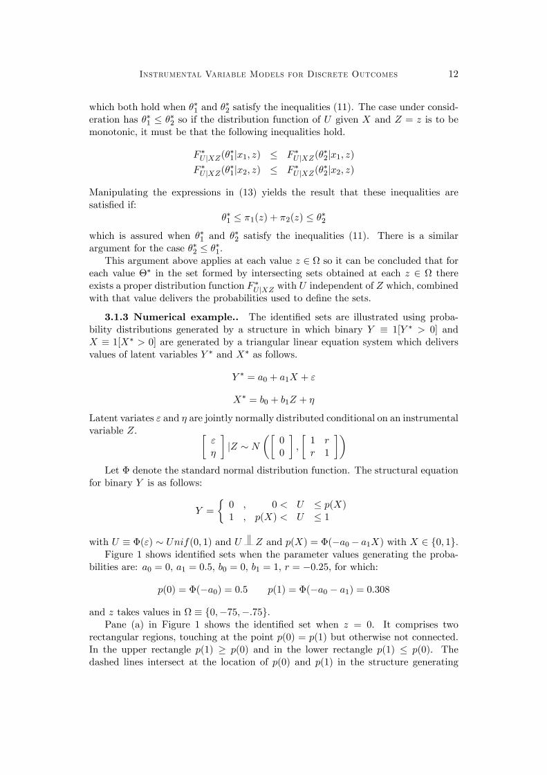
Figure 3 shows the set de�ned by the inequalities of Theorem 1 for the interceptand slope coe¢ cients, �0 and �1 in a 5 class model. The dark shaded set is obtainedwhen the instrument is relatively strong (b1 = 2). This set lies within the set obtainedwhen the instrument is relatively weak (b1 = 1). Figure 4 shows identi�ed sets(shaded) for these weak and strong instrument scenarios when there are 11 classesrather than 5. The 5 class sets are shown in outline. The e¤ect of reducing the

7The integrate procedure in R (Ihaka and Gentleman (1996)) was used to calculate probabilities.Intersection bounds over z 2 Z were obtained as in (6) using the R function optimise. The resultingprobability inequalties were inspected over a grid of values of � at each value of � considered, a valuebeing classi�ed as out of the identi�ed set as soon as a value of � was encountered for which therewas violation of one or other of the inequaltites (6). I am grateful to Konrad Smolinski for developingand programming a procedure to e¢ ciently track out the boundaries of the sets.


discreteness of the outcome is substantial and there is a substantial reduction in theextent of the set as the instrument is strengthened.

The sets portrayed here are outer regions which contain the sets identi�ed by themodel. The identi�ed sets are computationally challenging to produce in this con-tinuous endogenous variable case. Chesher and Smolinski (2009) investigate feasibleprocedures based on discrete approximations.

4. Concluding remarks

It has been shown that, when outcomes are discrete, single equation IV models do notpoint identify the structural function that delivers the discrete outcome. The modelshave been shown to have partial identifying power and set identi�cation results havebeen obtained. Identi�ed sets tend to be smaller when instrumental variables arestrong and have rich support and when the discrete outcome has rich support. Im-posing parametric restrictions reduces the extent of the identi�ed sets but in generalparametric restrictions do not deliver point identi�cation of the values of parameters.

To secure point identi�cation of structural functions more restrictive models arerequired. For example, specifying recursive structural equations for the outcome andendogenous explanatory variables and restricting all latent variates and instrumentalvariables to be jointly independently distributed produces a triangular system modelwhich can be point identifying.8 This is the control function approach studied inBlundell and Powell (2004), Chesher (2003) and Imbens and Newey (2009). Therestrictions of the triangular model rule out full simultaneity (Koenker (2005), Section8.8.2) such as arises in the simultaneous entry game model of Tamer (2003). Anadvantage of the single equation IV approach set out in this paper is that it allowsan equation-by-equation attack on such simultaneous equations models for discreteoutcomes, avoiding the need to deal directly with the coherency and completenessissues they pose.

The weak restrictions imposed in the single equation IV model lead to partialidenti�cation of deep structural objects which complements the many developmentsin the analysis of point identi�cation of the various average structural features studiedin for example Heckman and Vytlacil (2005).

There are a number of interesting extensions. For example the analysis can beextended to the multiple discrete outcome case such as arises in the study of paneldata. Consider a model for T discrete outcomes each determined by a structuralequation as follows:

Yt = ht(X;Ut); t = 1; : : : ; T

where each function ht is weakly increasing and càglàd for variations in Ut and eachUt is a scalar random variable normalised marginally Unif(0; 1) and U � fUtgTt=1and instrumental variables Z 2 are independently distributed. In practice therewill often be cross equation restrictions, for example requiring each function ht to bedetermined by a common set of parameters.

8But not when endogenous variables are discrete, Chesher (2005).


1.0 0.5 0.0 0.5 1.0

0.0

0.5

1.0

1.5

2.0

2.5

α0

α1

weak instrumentstrong instrument

Figure 3: Outer regions within which lie identi�ed sets for an intercept, �0, andslope co¢ cient, �1, in a 5 class ordered probit model with endogenous explanatoryvariable. The dashed lines intersect at the values of a0 and a1 used to generate thedistributions employed in this illustration.


1.0 0.5 0.0 0.5 1.0

0.0

0.5

1.0

1.5

2.0

2.5

α0

α1

weak instrumentstrong instrument

Figure 4: Outer regions within which lie identi�ed sets for an intercept, �0, andslope co¢ cient, �1, in a 11 class ordered probit model with endogenous explanatoryvariable. Outer regions for the 5 class model displayed in Figure 3 are shown inoutline. The dashed lines intersect at the values of a0 and a1 used to generate thedistributions employed in this illustration.


De�ne h � fhtgTt=1 and � � f� tgTt=1 and:

C(�) � Pr"T\t=1

(Ut � � t)#

which is a copula since the components of U have marginal uniform distributions. Anargument along the lines of that used in Section 2.1 leads to the following inequalitieswhich hold for all � 2 [0; 1]T and z 2 .

Pr

"T\t=1

(Yt � ht(X; � t))jZ = z#� C(�)

Pr

"T\t=1

(Yt < ht(X; � t))jZ = z#< C(�)

These can be used to delimit the sets of structural function and copula combinationsfh;Cg identi�ed by the model.

Other extensions arise on relaxing restrictions maintained so far. For exampleit is straightforward to generalise to the case in which exogenous variables appearin the structural function. In the binary outcome case additional heterogeneity, W ,independent of instruments Z, can be introduced if there is a monotone index restric-tion, that is if the structural function has the form h(X�;U;W ) with h monotonic inX� and in U . This allows extension to measurement error models in which observed~X = X +W . This can be further extended to the general discrete outcome case if amonotone index restriction holds for all threshold functions.

Acknowledgements

I thank Victor Chernozhukov, Martin Cripps, Russell Davidson, Simon SokbaeLee, Arthur Lewbel, Charles Manski, Lars Nesheim, Adam Rosen, Konrad Smolin-ski and Richard Spady for stimulating comments and discussions and referees forvery helpful comments. The support of the Leverhulme Trust through grants tothe research project Evidence Inference and Inquiry and to the Centre for Micro-data Methods and Practice (CeMMAP) is acknowledged. The support for CeMMAPgiven by the UK Economic and Social Research Council under grant RES-589-28-0001 since June 2007 is acknowledged. This is a revised and corrected version ofthe CeMMAP Working Paper CWP 05/07, �Endogeneity and Discrete Outcomes�.The main results of the paper were presented at an Oberwolfach Workshop on March19th 2007 Detailed results for binary response models were given at a conference inhonour of the 60th birthday of Peter Robinson at the LSE, May 25th 2007. I amgrateful for comments at these meetings and at subsequent presentations of this andrelated papers.


References

Beresteanu, Arie, Molchanov, Ilya and Francesca Molimari (2008): �SharpIdenti�cation Regions in Games,�CeMMAP Working Paper, CWP15/08.Berry, Steven and Elie Tamer (2006): �Identi�cation in Models of OligopolyEntry,� in Advances in Economics and Econometrics: Theory and Applications:Ninth World Congress, vol 2, R. Blundell, W.K. Newey and T. Persson, eds, Cam-bridge University Press.Chernozhukov, Victor And Christian Hansen (2005): �An IV Model of Quan-tile Treatment E¤ects,�Econometrica, 73, 245-261.Chernozhukov, Victor, Imbens, Guido W., and Whitney K. Newey (2007):�Instrumental Variable Estimation of Nonseparable Models,�Journal of Economet-rics, 139, 4-14.Chernozhukov, Victor, Lee, Sokbae And Adam Rosen (2008): �IntersectionBounds: Estimation and Inference,�unpublished paper, presented at the cemmap -Northwestern conference on Inference in Partially Identi�ed Models with Applications,London, March 27th 2008.Chesher, Andrew D., (2003): �Identi�cation in nonseparable models,�Economet-rica, 71, 1405-1441.Chesher, Andrew D.,(2009): �Single Equation Endogenous Binary Response Mod-els,�CeMMAP Working Paper, CWP16/09.Chesher, Andrew D., and Konrad Smolinski (2009): �Set Identifying Endoge-nous Ordered Response Models,�in preparation.Ciliberto, Federico and Elie Tamer (2009): �Market Structure and MultipleEquilibria in Airline Markets,�forthcoming in Econometrica.Heckman, J.J., and E. Vytlacil (2005): �Structural Equations, Treatment Ef-fects, and Econometric Policy Evaluation,�Econometrica, 73, 669-738.Ihaka, Ross, and Robert Gentleman (1996): �R: A language for data analysisand graphics,�Journal of Computational and Graphical Statistics, 5, 299-314.Imbens, Guido W., and Whitney K. Newey (2009): �Identi�cation and estima-tion of triangular simultaneous equations models without additivity,�forthcoming inEconometrica.Koenker, R.W., (2005): Quantile Regression. Econometric Society Monograph No.38. Cambridge University Press, Cambridge.Mullahy, John (1997): �Instrumental variable estimation of count data models:applications to models of cigarette smoking behavior,� Review of Economics andStatistics, 79, 586-593.Tamer, Elie (2003): �Incomplete Simultaneous Discrete Response Model with Mul-tiple Equilibria,�Review of Economic Studies, 70, 147-165.Windmeijer, Frank A.G., and João M.C. Santos Silva: (1997): �Endogeneityin count data models: an application to demand for health care,�Journal of AppliedEconometrics, 12, 281-294.


Annex

Proof of Theorem 3. Sharp set identi�cation for binary outcomes

The proof proceeds by considering a structural function h(x; u), that: (i) is weaklymonotonic non-decreasing for variations in u, (ii) is characterised by a thresholdfunction p(x), and (iii) satis�es the inequalities of Theorem 1 when probabilities arecalculated using a conditional distribution FY XjZ .

A proper conditional distribution FUXjZ is constructed such that U and Z are in-dependent and with the property that the distribution function generated by fh; FUXjZgis identical to FY XjZ used to calculate the probabilities in Theorem 1.

Attention is directed to constructing a distribution for U conditional on bothX and Z, FU jXZ . This is combined with FXjZ , the (identi�ed) distribution of Xconditional on Z implied by FY XjZ , in order to obtain the required distribution of(U;X) conditional on Z.

The construction of FUXjZ is done for a representative value, z, of Z. The argu-ment of the proof can be repeated for any z such that the inequalities of Theorem 1are satis�ed. It is helpful to introduce some abbreviated notation. At many pointsdependence on z is not made explicit in the notation.

Let denote the support of X conditional on Z. Y is binary taking values infy1; y2g. De�ne conditional probabilities as follows.

�1(x) � Pr[Y = y1jx; z]

�1 � Pr[Y = y1jz] =Z�1(x)dFXjZ(xjz)

and �2(x) � 1 � �1(x), �2 � 1 � �1 and note that dependence of , �1(x), �2(x),etc., on z is not made explicit in the notation.

A threshold function p(x) is proposed such that

Y =

�y1 ; 0 � U � p(x)y2 ; p(x) < U � 1

and this function satis�es some inequalities to be stated. The threshold function is acontinuous function of x and does not depend on z.

De�ne the following functions which in general depend on z.

u1(v) = min(v; �1) u2(v) = v � u1(v)

De�ne sets as follows:

X(s) � fx : p(x) = sg X[s] � fx : p(x) � sg

and let � denote the empty set. De�ne

s1(v) � mins

(s :

Zx2X[s]

�1(x)dFXjZ(xjz) = u1(v))


and:

s2(v) � mins

(s :

Zx2X[s]

�2(x)dFXjZ(xjz) = u2(v))

and de�ne functions �1(v; x) and �2(v; x).

�1(v; x) ��1(x) ; x 2 X[s1(v)]0 ; x =2 X[s1(v)]

�2(v; x) ��2(x) ; x 2 X[s2(v)]0 ; x =2 X[s2(v)]

For a structural function h(x; u) characterized by the threshold function p(x) andfor a probability measure that delivers �1(x) and FXjZ , a distribution function FU jXZis de�ned as

FU jXZ(ujx; z) � �(u; x) � �1(u; x) + �2(u; x)

where z is the value of Z upon which there is conditioning at various points in thede�nition of �(u; x).

Consider functions p that satisfy the inequalities of Theorem 1 which in this binaryoutcome case can be expressed as follows.

for all u 2 (0; 1) :Z

p(x)<u

�1(x)dFXjZ(xjz) < u � �1 +Z

p(x)<u

�2(x)dFXjZ(xjz) (A1)

It is now shown that:

1. for all x and any z the distribution function �(u; x) is proper: (a) �(0; x) = 0,(b) �(1; x) = 1, (c) for v0 > v �(v0; x) � �(v; x).

2. there is an independence property:

for all uZx2

�(u; x)dFXjZ(xjz) = u

3. if p satis�es the inequalities (A1) then there is an observational equivalenceproperty: for all x

�(p(x); x) = �1(x):

(1a). Proper distribution: �(0; x) = 0.

By de�nition u1(0) = u2(0) = 0 and so s1(0) = s2(0) = 0. Therefore X[s1(0)] =X[s2(0)] = � which implies that, for all x, �1(0; x) = �2(0; x) = 0 and so �(0; x) = 0.

(1b). Proper distribution: �(1; x) = 1.

By de�nition u1(1) = �1, so s1(1) is the smallest value of s such that X[s] = so s = maxx2 p(x). With X[s1(1)] = it is assured that �1(1; x) = �1(x) for all x.

By de�nition: u2(1) = �2, so s2(1) is the smallest value of s such that X[s] = .With X[s2(1)] = it is assured that �2(1; x) = �2(x) for all x. So, for all x,�(1; x) = �1(x) + �2(x) = 1.


(1c). Proper distribution: nondecreasing �(u; x).

Since u1(v) and u2(v) are nondecreasing functions of v, so are s1(v) and s2(v). Itfollows that for v0 > v

X[s1(v0)] � X[s1(v)] X[s2(v

0)] � X[s2(v)]

and so for all x�1(v

0; x) � �1(v; x) �2(v0; x) � �2(v; x)

and it follows that the sum of the functions, �(v; x), is a nondecreasing function of v.

(2). Independence.

By de�nitionZx2

�1(v; x)dFXjZ(xjz) =Z

x2X[s1(v)]

�1(x)dFXjZ(xjz) = u1(v)

Zx2

�2(v; x)dFXjZ(xjz) =Z

x2X[s2(v)]

�2(x)dFXjZ(xjz) = u2(v)

and so Zx2

�(v; x)dFXjZ(xjz) = u1(v) + u2(v) = v

which does not depend upon z.

(3). Observational equivalence.

This requires that for all x: �(p(x); x) = �1(x) which is true if for all x: (a)�1(p(x); x) = �1(x) and (b) �2(p(x); x) = 0. Each equation is considered in turn.The inequalities (A1) come into play.

(a) �1(p(x); x) = �1(x).Since for all u Z

p(x)<u

�1(x)dFXjZ(xjz) < u

there exists �(u) > 0 such thatZp(x)<u+�(u)

�1(x)dFXjZ(xjz) = u

for all u � �1.It follows that s1(v) > v for all v which implies X[v] � X[s1(v)] and in particular

X(v) � X[s1(v)].For some value of x, x�, de�ne p� � p(x�). Then for p� 2 (0; 1),

X(p�) � fx : p(x) = p�g � X[p�] � X[s1(p�)]:


Recall that �1(v; x) is equal to �1(x) for all x 2 X[s1(v)]. It has been shown that forany p�, all x such that p(x) = p� lie in the set X[s1(p�)] and so �1(p

�; x�) = �1(x�)and there is the result �1(p(x); x) = �1(x).

(b) �2(p(x); x) = 0.Recall X(v) � fx : p(x) = vg. It is required to show that X(v) \ X[s2(v)] is

empty for all v.Since u2(v) = 0 for v � �1, s2(v) = 0 for v � �1 and X[s2(v)] = � for v � �1.

Therefore, for v � �1

X(v) \X[s2(v)] = X(v) \ � = �.

From (A1) there is the following inequality.Zp(x)<v

�2(x)dFXjZ(xjz) � v � �1

For v > �1, the constraint implies that there exists (v) � 0 such thatZp(x)<v� (v)

�2(x)dFXjZ(xjz) = v � �1

and, since for v > �1

s2(v) � mins

(s :

Zp(x)<s

�2(x)dFXjZ(xjz) = v � �1

)

it follows that s2(v) < v. It follows that for v > �1, X(v) \ X[s2(v)] = � becausewith s2(v) < v:

fx : p(x) < s2(v)g \ fx : p(x) = vg = �

De�ne p� = p(x�). Then for p� 2 (0; 1), X(p�) \X[s2(p�)] = � so �2(p�; x�) = 0and there is the result, for all x, �2(p(x); x) = 0:

Documents

Instrumental variable models for discrete outcomes · 2009-08-18 · Instrumental Variable Models for Discrete Outcomes 3 comparison with the single equation instrumental variable