instructor Matteo Pozzi - Carnegie Mellon University

Lec. 0212735: Urban Systems Modeling Probability

12735: Urban Systems Modeling

instructor: Matteo Pozzi

1

Probability

Lec. 02


outline

‐ what is probability;‐ discrete and continuous random variables;‐ distribution of random variables, functions of random variables;‐ first and second moments of random variables;‐ uni‐variate distribution models: normal, log‐normal, exponential;‐ multiple random variables;‐ joint, marginal, conditional distributions; ‐ multi‐variate distribution models.

2


PART I

uni‐variate distribution models

3


probability

4

P Probability of event A.

P Probability of event B.

P ∨ Probability of event A or event B.

P , Probability of event A and event B.

P ∨ P P P ,P ∨ 1 ⇒ P 1 P

∨

,

http://earthquake.usgs.gov/regional/nca/ucerf/

Venn diagram

P ∨P P

If P , 0Disjoint events:

0 P ∙ 1


what is probability?

5

http://www.digii.eu/2011/20110703‐15‐holiday‐in‐campervan‐to‐italy‐and‐france/20110712‐leaning‐tower‐of‐pisa/sx19774‐marijn‐pushing‐down‐leaning‐tower‐of‐pisa‐italyjpg

10%

90%

https://userexperience.jux.com/#791734

P lim→

#

frequentist viewstochastic process:

estimate probability by a finite sample

P :

Bayesian probability

‘degree of belief’ in event

rational agent: set of consistent beliefs

with probability calculuswith decision making


random variables

6

realityit evolves deterministically.

perceptionincomplete observations, incomplete understanding of the system dynamics.

probability is a complete representation of incomplete knowledge.

value[number]

random variable[distribution]

0 5 100

0.2

0.4

x

p(x)

0 5 10x

3.25


from events (and experiments) to random variables

7

http://commons.wikimedia.org/wiki/File:Dice.png

6 possible outcomes

http://forum.skyscraperpage.com/showthread.php?t=183620 Venn diagram

Ensemble:

for event , we can define as a binary random variable:

1 w. p. P 0 w. p. P 1 P

; ;

1

4

2 3

5 6

Venn diagram

random variable

domaindistribution

complete set of mutually exclusive events

We assign numerical values (in ) to each possible outcome of an experiment.

experiment on a discrete domain


discrete random variables

8

1 2 3 40

0.05

0.1

0.15

0.2

0.25

0.3

0.35

X

P(X

)

1

18% 29% 38% 15%

≜ P 0

∀ : P , 0mutually exclusive outcomescomplete setP ∨ ⋯∨ 1

3 1 2 3 85%

normalized

1, 2, 3, 4

1 2 3 40

0.5

1

X

F(X

)

≜ P

positive

probability distribution:

cumulative probability distribution:

, , . . , discrete domain

example


continuous random variables

9

[Bishop, 2006]

0

1

Probability Density Function

≜ lim→

P ∈ , ΔΔ

P ∈ , Δ ≅ Δ

P ∈ ,Cumulative Density Function

≜ P ∈ ∞,

∈ 0,1

0 P ∈ ,

normalized:

non‐negative:P ∈ ,


expectation and moments

10

Expectation of function of a random variable

discrete continuous

Linearity of expectation

x

p(x)

, f(x

)

p(x)f(x)

proof

expectation of a constant is the constant itself

original variable: variable derived by deterministic function:mean of derived variable :


expectation and moments

11

≜ ≜

≜ var

≜

First moment (mean value) [ i.e. expectation for ]

Second moment around the mean (aka variance)

coefficient of variation


discrete continuous

discrete continuous

standard deviation

x

p(x)

x

p(x)

≜ → from linearity of expectation

Linear transformation of a random variable

x

p(x)

, f(x

)

p(x)f(x)


characterization of a random variable

12

0 5 10 150

50

xo

E [

(x -

x o)2 ]

Chebyshev’s inequality

P1≜

2 2 3 4

50% 25% 11% 6.2%

mode: ≜ argmax

median: : 50%

mean as “best guess” for expected norm‐2 error:

argmin

0 5 10 15

0

0.05

0.1

0.15

0.2

0.25

0.3

0.35

p(x)

mode mean

mean std

0

0.5

1

x

F(x) median Relation between

moments and tails:


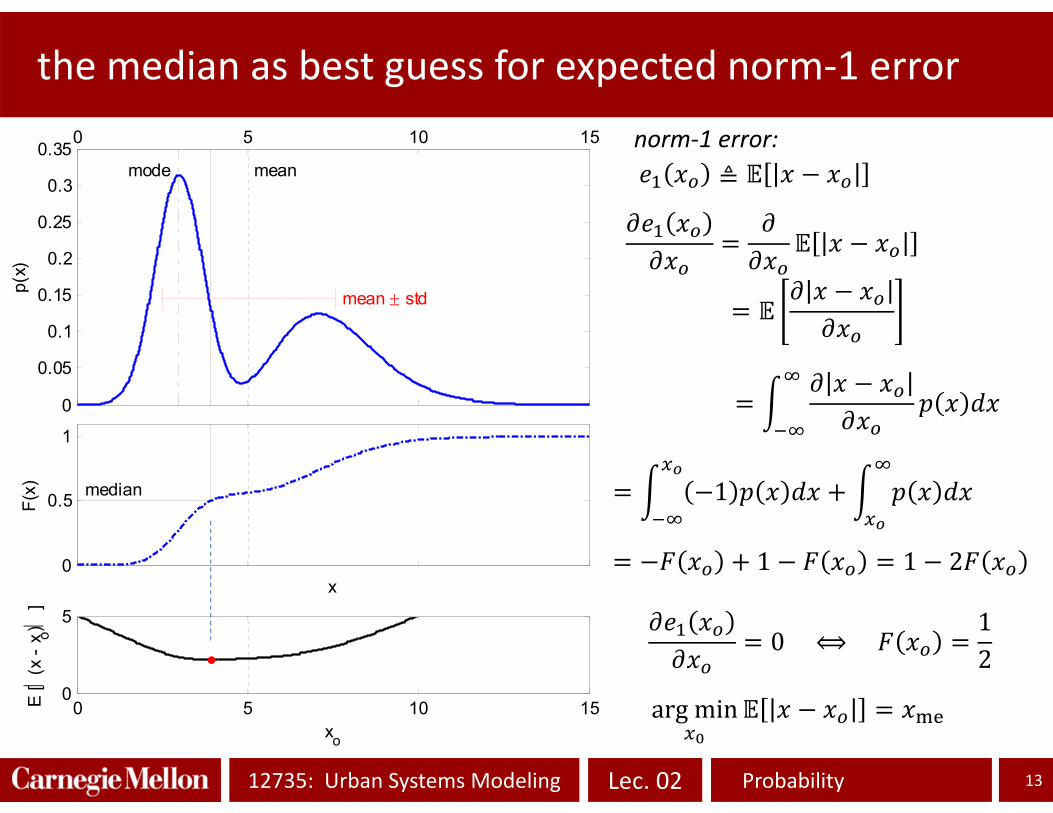
the median as best guess for expected norm‐1 error

13

0 5 10 15

0

0.05

0.1

0.15

0.2

0.25

0.3

0.35

p(x)

mode mean

mean std

0

0.5

1

x

F(x) median

0 5 10 150

5

xo

E [

(x -

x o) ]

≜

1

1 1 2

0 ⟺ 12

norm‐1 error:

argmin


transformation of random variables

14

,,

′

≜

x

p x(x) ,

Fx(x

)

0

1

x

z

z = f(x)

x = f -1(z) = g(z)

px(x)

Fx(x)

)

)

random variable

transformation

: monotonically increasing

new random variable

P ∈ ∞, P ∈ ∞,

taking derivative:

inverse

note that:

equal probability:

pz(z) , Fz(z)

z

pz(z)

Fz(z)


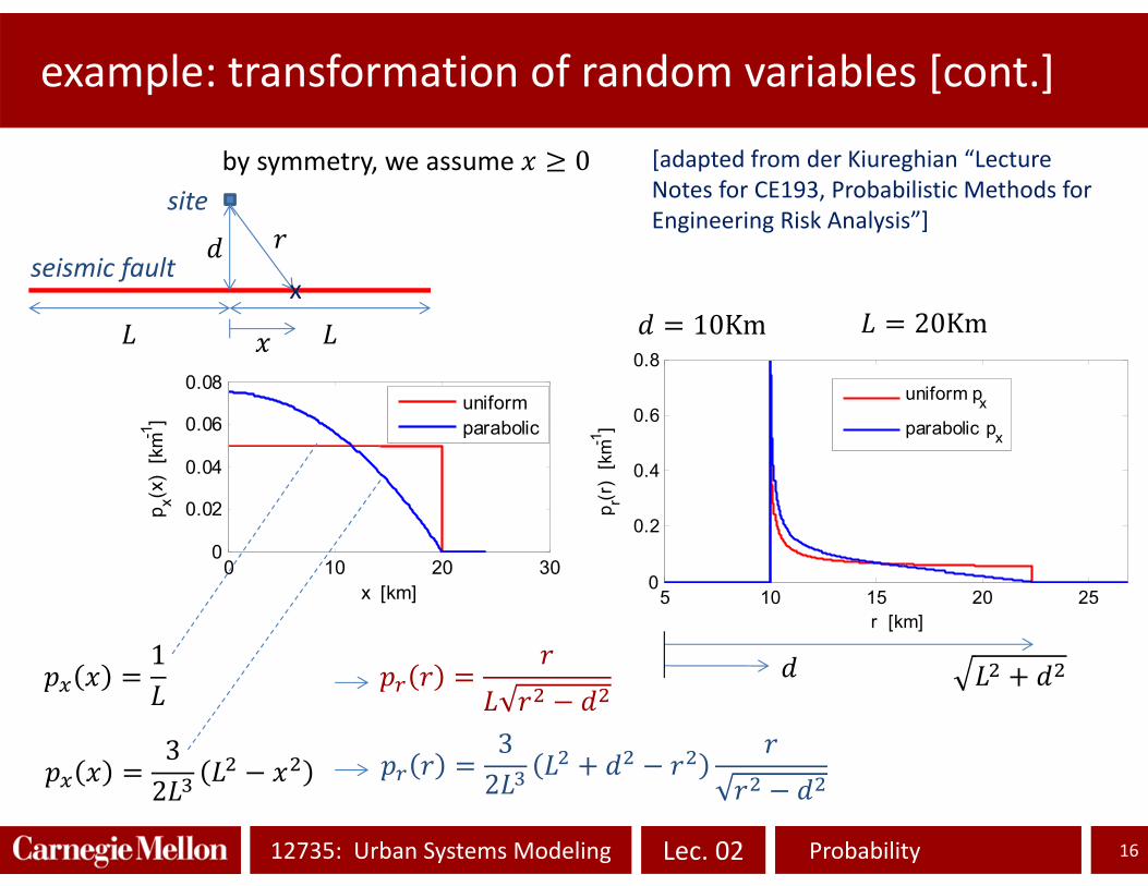
example: transformation of random variables

15

′

∈ 0,

1

32 0 otherwise

0 10 20 300

0.02

0.04

0.06

0.08

x [km]

p x(x)

[km-1

]

uniformparabolic

seismic fault

site

x

epicenter position source to site distance

by symmetry, we assume 0

32


example: transformation of random variables [cont.]

16

20Km10Km

5 10 15 20 250

0.2

0.4

0.6

0.8

r [km]p r(r

) [k

m-1]

uniform px

parabolic px

[adapted from der Kiureghian “Lecture Notes for CE193, Probabilistic Methods for Engineering Risk Analysis”]

32

0 10 20 300

0.02

0.04

0.06

0.08

x [km]

p x(x)

[km-1

]

uniformparabolic

seismic fault

site

x

by symmetry, we assume 0

1

32


normal distribution

17

; , ≜12

exp12 ; , 0

; , 1; , ⇒ ; varx

p(x)

2

‐ Symmetrical distribution (around the mean);‐ : position‐ : uncertainty

‐ mean = mode = median [= ]

Pdf:

http://en.wikipedia.org/wiki/Normal_distribution


normal distribution [cont.]

18

log ; ,12

0

0.5

1

x

F(x)

2

x

p(x)

2

log

[p(x

)] Φ ; , ≜ ; ,

; , ≜12

exp12 ; , 0

; , 1; , ⇒ ; var

Pdf:

Cdf:

Φ ; ,12

Φ ; ,12

12 Φ ; ,

anti‐symmetry

parabola in log‐scale


standard normal distribution

19

′

Φ12

exp 2

-3 -2 -1 0 1 2 30

0.5

1

z

(z

)

; , ≜12

exp12Pdf:

transformation:

12

exp 2 ; 0,1

Φ ≜ Φ ; 0,1

standard normal pdf:

standard normal cdf:

Φ ; , Φtrasformation for cdf:

≜12

exp 2

-3 -2 -1 0 1 2 3

0

0.1

0.2

0.3

0.4

z

(z)


linear transformation of a normal random variable

20

′

1

; , ≜1

2exp

12

Pdf:

linear transf.:

1

2exp

12

1

-2 0 2 4 6 8 100

0.5

1

x, y

F x(x),

F y(y)

-2 0 2 4 6 8 10

0

0.1

0.2

0.3

0.4

x, y

p x(x),

p y(y)

=0 ; =1=1 ; =1.5=2 ; =2

; ,

the linear transformation of a normal RV is still a normal RV. The transformation of the parameters follows the rule of transformation for first and second moment.


log‐normal distribution

21

explog

1

12

exp12 log 0

0 0≜ ln ; ,

exp 2

; ,12

exp12

exp 1

ln 1 ≅ ; ln 2 ≅ ln -1 0 1 2

x

p x(x) ,

Fx(x

)

=E(x)

1

0

x

y

y = exp(x)x = log(y)

0

1

2

3

4

5

py(y) , Fy(y)

y

E(y)exp()

1

0

var exp 1 exp 2

moments:

approximation: ≪ 1 → ≅ exp ; ≅

inverse relations:


log‐normal distributiont [cont.]

22

explog

1

12

exp12 log 0

0 0≜ ln ; ,

; ,12

exp12

‐ Asymmetrical distribution;‐ only positive values are

possible.‐ For small cov ( 1), log‐

normal is similar to normal.

Φ

‐ Cumulative distribution:0 1 2 3 4 5 6 7 8 9 10

0

0.1

0.2

0.3

0.4

0.5

0.6

0.7

z

p(z)

=2, =0.1=1, =0.5=1, =1.5

2 2.2 2.4 2.6 2.8 3 3.2 3.4 3.6 3.8 40

2

4

z

p(z)

logn, =1, =0.05norm, =exp()=2.72, ==0.136


0 5 10 15

0

0.05

0.1

0.15

0.2

0.25

p(y)

[m

-1]

0 5 10 150

0.5

1

y [m]

F(y)

0 5 10 15

0

0.05

0.1

0.15

0.2

0.25

p(y)

[m

-1]

0 5 10 150

0.5

1

y [m]

F(y)

example: design of a levee

23

: height of water level ln ; , 6m var 2m11m: height of barrier P ?

1 Φlog

2.1%

33.3% ln 1 32.4% ln 2 1.74 ln 1.79

P 1

Find ∗: P ∗ 5%∗ exp ∙ Φ 1

: st. normal: normal

: log‐normal9.71m

2.1%5.0%

http://www.zmescience.com/ecology/environmental‐issues/levees‐at‐work‐against‐mississippi‐flood‐4234323/

∗


exponential distribution

24

-1 0 1 2 3 4 50

0.2

0.4

0.6

0.8

1

x []

p(x)

, F

(x)

p(x)F(x)

1 exp 00 0

; ≜ exp 00 0

Pdf:

Cdf:

1

1

var1

moments:

1application: if events occurs following a Poisson process with rate , then the inter‐arrival time is exponential with .


PART II

multi‐variate distribution models

25


joint, marginal, conditional probability

26

Two random variables: and .

example: : force applied to a structure during an exceptional event.: damage experienced by a structure

what is , [marginal probability] e.g. what is the prob. of high force?what is , [joint probability] e.g. what is the prob. of high force

AND mild damage?what is [conditional probability] e.g. what is the prob. of severe

damage GIVEN low force?what is [conditional probability] e.g. what is the prob. of high force

GIVEN high damage?

the pair , : is a complete representation of this small “world”.

queries:

Y ′severe damage′ X ′low force′X ′low force′, Y ′severe damage′

X ′low force′

conditional probability :

marginal probability :

Y ′severe damage′ X ′low force′, Y ′severe damage′ ⋯X ′high force′, Y ′severe damage′

mutually exclusive events


Y 1 Y 2 Y 3 Y 4 Y 5 Y 6 Y 1 Y 2 Y 3 Y 4 Y 5 Y 6

X 1 2.1% 5.6% 4.2% 3.5% 2.1% 0.7% 18.2% 11.5% 30.8% 23.1% 19.2% 11.5% 3.8% 100%X 2 2.8% 4.9% 7.0% 6.3% 4.9% 2.8% 28.7% 9.8% 17.1% 24.4% 22.0% 17.1% 9.8% 100%X 3 1.4% 4.2% 9.1% 12.6% 7.0% 3.5% 37.8% 3.7% 11.1% 24.1% 33.3% 18.5% 9.3% 100%X 4 0.7% 1.4% 2.8% 3.5% 4.9% 2.1% 15.4% 4.5% 9.1% 18.2% 22.7% 31.8% 13.6% 100%

7.0% 16.1% 23.1% 25.9% 18.9% 9.1%

X 1 30.0% 34.8% 18.2% 13.5% 11.1% 7.7%X 2 40.0% 30.4% 30.3% 24.3% 25.9% 30.8%X 3 20.0% 26.1% 39.4% 48.6% 37.0% 38.5%X 4 10.0% 8.7% 12.1% 13.5% 25.9% 23.1%

100% 100% 100% 100% 100% 100%

probability tables

27

,

,: tables, dimension

: vector, dimension 1

: vector, dimension 1

Joint probability:

,,

, 0 ,,

1

Marginal probability:

Conditional probability:, ,

,


Y 1 Y 2 Y 3 Y 4 Y 5 Y 6 Y 1 Y 2 Y 3 Y 4 Y 5 Y 6

X 1 2.1% 5.6% 4.2% 3.5% 2.1% 0.7% 18.2% 11.5% 30.8% 23.1% 19.2% 11.5% 3.8% 100%X 2 2.8% 4.9% 7.0% 6.3% 4.9% 2.8% 28.7% 9.8% 17.1% 24.4% 22.0% 17.1% 9.8% 100%X 3 1.4% 4.2% 9.1% 12.6% 7.0% 3.5% 37.8% 3.7% 11.1% 24.1% 33.3% 18.5% 9.3% 100%X 4 0.7% 1.4% 2.8% 3.5% 4.9% 2.1% 15.4% 4.5% 9.1% 18.2% 22.7% 31.8% 13.6% 100%

7.0% 16.1% 23.1% 25.9% 18.9% 9.1%

relations between probability tables

28

,

,

,product (chain) rule

definition of conditional

1

, ∑ ,1[ proof:

jointmarginalconditional

jointmarginal

conditional

]

“everything follows from the joint”

“you can build the joint…”


12

34

12

34

56

0

0.02

0.04

0.06

0.08

0.1

0.12

Y

X

P(X

,Y)

12

34

12

34

56

0

0.05

0.1

0.15

0.2

0.25

0.3

Y

XP

(Y

X)

relations among joint, marginal, conditional probability

29

,,

1

,,

,

1 2 3 40

0.2

X

P(X

)

1 2 3 4 5 60

0.1

0.2

Y

P(Y

)

,

1


Rules: sum, product, Bayes’ formula

30

,

Sum Rule

Product [chain] Rule,

Conditional≜

,

,

X Y

X Y

Bayes’ Rule

arc reversal

models for ,

: force : damage

products

damage force

force

force damage

e.g.: input

vulnerabilityinference


independency

31

: number of leaves on a tree in Japan

http://entertainmentguide.local.com/meaning‐japanese‐tree‐art‐10785.html

: number of cracks on the R. Clemente Bridge

http://en.wikipedia.org/wiki/File:Pittsburgh_Tenth_Street_Bridge_from_Bluff_downsteam.JPG

⟺

⟺ independent of :

,

,

the joint derives by the marginal probs.

X Y


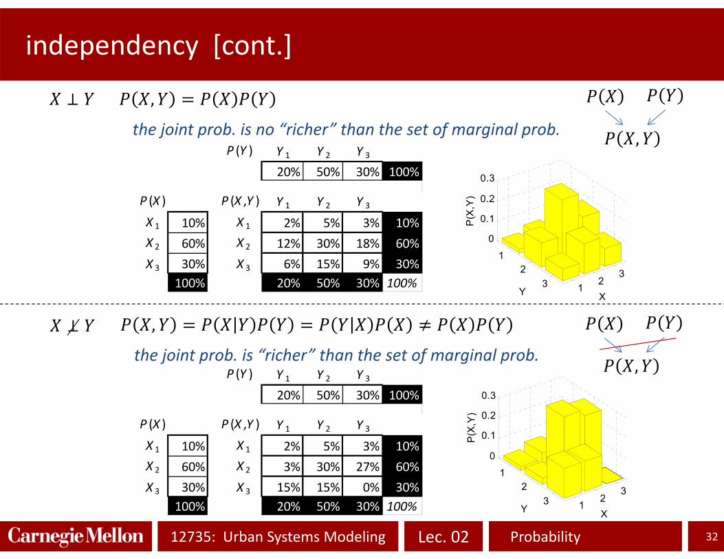
P (Y ) Y 1 Y 2 Y 3

20% 50% 30% 100%

P (X ) P (X ,Y ) Y 1 Y 2 Y 3

X 1 10% X 1 2% 5% 3% 10%X 2 60% X 2 3% 30% 27% 60%X 3 30% X 3 15% 15% 0% 30%

100% 20% 50% 30% 100%

P (Y ) Y 1 Y 2 Y 3

20% 50% 30% 100%

P (X ) P (X ,Y ) Y 1 Y 2 Y 3

X 1 10% X 1 2% 5% 3% 10%X 2 60% X 2 12% 30% 18% 60%X 3 30% X 3 6% 15% 9% 30%

100% 20% 50% 30% 100%

independency [cont.]

32

,

,

,

,the joint prob. is “richer” than the set of marginal prob.

the joint prob. is no “richer” than the set of marginal prob.

12

3

12

3

0

0.1

0.2

0.3

XY

P(X

,Y)

12

3

12

3

0

0.1

0.2

0.3

XY

P(X

,Y)


O,G ¬O,GE,G 0.6% 2.4% 3%¬E,G 1.4% 15.6% 17%

2% 18%

O,¬G ¬O,¬GE,¬G 2.4% 9.6% 12%¬E,¬G 5.6% 62.4% 68%

8% 72%

example of risk assessment with binary rand. var.s

33

E 15%O 10%

E O 2 E 30%

E, O E O O 30%10% 3%

E, O E E, O 15% 3% 12%

G 20% independent of Electricity, Oil

E, O O E, O 10% 3% 7%

E, O O E, O 90% 12% 78%

E 1 E 85%O 1 O 90%

E, O, G E, O G 62.4%

O ¬OE 3% 12% 15%¬E 7% 78% 85%

10% 90%

1 E, O, G 37.6%

G 1 G 80%

Shortage ofElectricity

Oil

reliability:dependency:

1 E, O 22%

GasReliability:

, , G, G

, , G, G

same results using P ∨ P P P ∙ P


curse of dimensionality

34

⋮

: 1, … ,

: 1, … ,

: 1, … ,⋮

# ∙ ⋯∙

number of “bins” for each dimension

∀ : 20

[Bishop, 2006]

→ # 201 2 3 4 5 6 7

101

103

105

107

109

# rv.s

# X


multivariate continuous distributions

35

x1

x 2

0 0.2 0.4 0.6 0.8 10

0.1

0.2

0.3

0.4

0.5

0.6

0.7

0.8

0.9

1

, ≜ lim→

P ∈ , Δ , ∈ , ΔΔ

joint distribution:

00.2

0.40.6

0.81

0

0.5

10

2

4

6

8

10

12

x1x2

p(x 1,x

2)

contour plot:zero on the borders

, 0

, 1

positive

normalizedmaximum


multivariate continuous distributions [cont.]

36

00.2

0.40.6

0.81

0

0.5

10

2

4

6

8

10

12

p(x2)

x1

p(x1,x2=0.45)p(x1=0.35,x2)

x2

p(x1)

p(x 1,x

2)

x1

x 2

0 0.2 0.4 0.6 0.8 10

0.1

0.2

0.3

0.4

0.5

0.6

0.7

0.8

0.9

1

, , 0

, 1

,

,

, ,

marginal distributions:joint distribution:

conditional:contour plot:

positive

normalized


multivariate continuous conditional distributions

37

00.2

0.40.6

0.81

0

0.5

10

2

4

6

8

x1x2

p(x 2

x 1)

00.2

0.40.6

0.81

0

0.5

10

1

2

3

4

5

x1x2

p(x 1

x 2)

, ,conditional:

, , 0

, 1

,

,

marginal distributions:joint distribution:

positive

normalized


independency

38

, chain rule, it always holds

⇒ , ⇒

[⟺ ]

x1

x 2

0 0.2 0.4 0.6 0.8 10

0.1

0.2

0.3

0.4

0.5

0.6

0.7

0.8

0.9

1

00.2

0.40.6

0.81

0

0.5

10

2

4

6

8

10

p(x2)

x1

p(x1,x2=0.17)p(x1=0.225,x2)

x2

p(x1)

p(x 1,x

2)

contour plot:


independency [cont.]

39

, chain rule, it always holds

⇒ , ⇒

[⟺ ]

0

0.5

1

0

0.5

10

0.5

1

1.5

2

2.5

3

x1x2

p(x 2

x 1)

0

0.5

1

0

0.5

10

0.5

1

1.5

2

2.5

3

x1x2

p(x 1

x 2)


expectation, first and second moments

40

≜ , ,


continuous [same for discrete]

Linearity of expectation still holds

≜

≜

, ,

≜ var

≜ var

≜

first and second moments

covariance

0 if ⇢ ; ⇢ ;0 if ⇢ ; ⇢ ;

sign of covariance

if a function depends on only, we can compute using the marginal on .


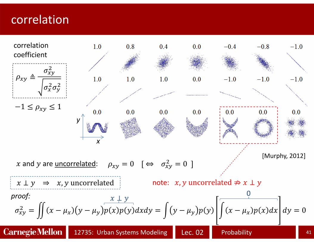
correlation

41

≜

1 1

[Murphy, 2012]

correlationcoefficient

x

y

0 ⇔ 0and are uncorrelated:

⇒ , uncorrelated

0

note: , uncorrelated ⇏

0proof:


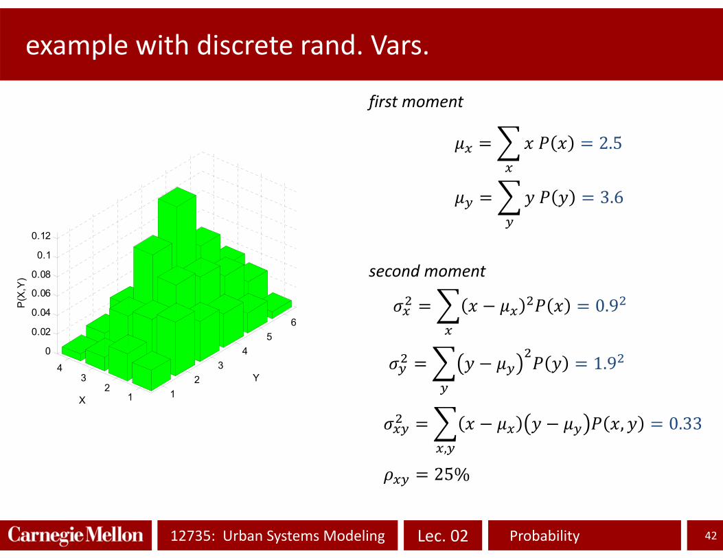
example with discrete rand. Vars.

42

12

34

12

34

56

0

0.02

0.04

0.06

0.08

0.1

0.12

Y

X

P(X

,Y)

25%

0.9

,,

0.33

2.5

3.6

1.9

first moment

second moment


vector notation, moments for multivariate rand. vars.

43

, , … ,⋮

⋮

≜ ;

……

⋮ ⋮ ⋱ ⋮…

00

… 0… 0

⋮ ⋮0 0

⋱ ⋮…

11

……

⋮ ⋮ ⋱ ⋮… 1

00

… 0… 0

⋮ ⋮0 0

⋱ ⋮…

vector of rv.s joint probability

dimension: 1

⟶ 1

first moment: mean vector

second moment: covariance matrix

«correlation matrix»diagonal matrix of standard deviation

positive and normalized

variance on the diagonal

covariance out the diagonal

1


expectation for multi‐variate rand. var.s

44

Expectation of function of a vector of random variables

continuous

Linearity of expectation

≜ →

Linear transformation

: ⟶

dimension: ∶ 1 :

: 1

≜

≜

proofs for linear transformation:

∶∶ 1


expectation for multi‐variate rand. var.s

45

≜ → 0

Linear uni‐variate function (hyper‐plane): ⟶

properties of covariance matrix:

symmetry: positive definiteness: ∀ ∈ : 0

x1

x 2

0 0.5 10

0.5

1

x1

x 2

0 0.5 10

0.2

0.4

0.6

0.8

1

00.5

1

0

0.5

1-5

0

5

x1x2

y

≜ →

Linear transformation


refereces

46

on wikipedia:Probability interpretations ‐ Frequentist probability ‐ Probability axioms ‐Bayesian probability ‐ Random variable ‐ Normal distribution ‐ Log‐normal distribution ‐ Exponential distribution ‐ Joint probability distribution ‐ Conditional probability ‐ Marginal distribution ‐ Independence (probability theory)

Kroese D.P., A Short Introduction to Probability, Downloadable form www.maths.uq.edu.au/~kroese/asitp.pdf

MacKay, D. (2003). Information Theory. Inference and Learning Algorithms. Cambridge University Press. Downloadable from http://www.inference.phy.cam.ac.uk/mackay/itila/ch2, pg.22‐32

Pictures from:Bishop, C. (2006). Pattern Recognition and Machine Learning. SpringerMurphy, K. (2012). Machine Learning, a probabilistic perspective. MIT press.


MW Matlab ‐ commands

47

sum(v) : sum of the components of vector ‘v’.

p=normpdf(y,mu,sigma) : normal pdf, with mean mu and st.dev. sigma, at y.F=normcdf(y,mu,sigma) : normal cdf, with mean mu and st.dev. sigma, at y.p=pdf(‘logn’,y,lambda,zeta) : log‐normal pdf, with parameters lambda and zeta, at y.F=cdf(‘logn’,y,lambda,zeta) : log‐normal cdf, with parameters lambda and zeta, at y.z=norminv(F) : inverse standard normal cdf, computed at F.

bar(v) : bar plot of vector ‘v’. bar3(M) : bar plot of matrix ‘M’. plot(vx,vy) : plot of lines connecting points in vectors ‘vx’ (x‐coordinates) and ‘vy’ (y‐

coord.)surf(vx,vy,M) : surface plot of grid with x‐coordinates (‘vx’) and y‐coordinates (‘vy’),

defined in matrix ‘M’.contour(vx,vy,M) : surface plot of grid with x‐coordinates (‘vx’) and y‐coordinates (‘vy’),

defined in matrix ‘M’.

Documents

instructor Matteo Pozzi - Carnegie Mellon University