On Institutional Trading and Behavioral Bias

Sugato Chakravarty Purdue University

812 West State Street West Lafayette, IN 47906 Phone: (1) 765 494 6427

Email: Sugato@purdue.edu

and

Rina Ray University of Colorado Denver

1475 Lawrence St Denver, CO 80202

Phone: (1) 303 315 8465 Email: rina.ray@ucdenver.edu

Keywords: behavioral bias, institutional investors, liquidity, skill, transaction cost

JEL Code: G02, G11, G23

___________________________________

We would like to thank Byoung-min Kim for his enthusiastic research and computational assistance. We also thank V. Ravi Anshuman, S.G. Badrinath, Jonathan Bauchet, Bidisha Chakrabarty, Lee Cohen, Werner De Bondt (discussant), Pankaj Jain, Christine Jiang, Huseyin Gulen, Ron Laschever, Sandra Mortal, Srinivasan Rangan, Tom McInish, Shashidhar Murthy, Venky Panchapagesan, Chuck Trzcinka, Rob Van Ness, Bonnie Van Ness, the Fogelman finance area doctoral students, as well as the doctoral students at Memphis, Old Miss and IIM Bangalore, the seminar participants at Purdue, the University of Connecticut, the University of Memphis, Wilfrid Laurier University, the Indian Institute of Management at Bangalore and, in for their comments.

1  

Abstract

Are institutional investors skilled at short-term trading or do they trade too much? Using historical cost

method, two recent studies provide contradictory answers to this question. The first suggests that

institutions are skilled and earn 26-34 basis points higher benchmark-adjusted returns for their buy trades

than sell trades. The second argues that the institutional fund managers earn -57 to -225 basis points

benchmark-adjusted return on their short-term trades and investors in these funds would have been better

off had these managers traded less. When we use a marked-to-market based fair value method – instead of

the historical cost method – for measuring fund manager skills, we find that institutional managers make

economically insignificant -4 to +9 basis points net profit on their short-term portfolio of buy – sell

transactions. The negative net marked-to-market profit comes exclusively from trades with 1-day holding

period. We find no evidence of overconfidence, biased self-attribution, or disposition effect among

institutional investors. Pension fund managers outperform money managers. Institutions engage in short-

term trades despite earning net zero return for liquidity, tax-minimization, risk-management, and window-

dressing reasons. Among these non-profit maximizing rational motives for trading, liquidity trading motive

is the strongest.

2  

Are institutional traders skilled or do they trade too much? Why do institutional investors trade equities

and how much trading constitutes too much? We expect institutions to trade primarily in order to maximize

risk-adjusted net portfolio return and when marginal benefit from trading exceeds the marginal cost,

including the opportunity cost of not trading and passively holding a market or benchmark portfolio.1 If

portfolio managers are able to do that, we infer that the managers are skilled at trading. Indeed, Puckett

and Yan (2011) find a large number of representative institutions – both money managers and pension fund

managers – earned 26 to 34 basis points higher benchmark-adjusted return after transaction cost on their

buy trades than on their sell trades within the quarter from 1999 to 2005. They take this as evidence of

“interim” trading-skill for institutions. Chakrabarty, Moulton, and Trzcinka (2017), on the other hand,

present starkly different results – raw (benchmark-adjusted) return of -82 to -337 ( -57 to -225) basis points

before transaction cost for trades with 1-day to 3-month holding period between 1999 and 2009. Both these

studies use the “historical cost” based accounting method for measuring fund manager performance.

A vast accounting and finance literature exist on the superior reliability and value-relevance of the

marked-to-market based “fair-value” accounting method over the “historical cost” method for valuation of

available for sell financial securities. Proponents of fair value method argue that gains and losses in fair

value securities are value relevant; that the fair value estimates are less biased and more informative than

the historical cost based estimates; and that fair value estimates of securities held by banks provide

significant explanatory power over security values estimated based on historical cost but the reverse is not

true (Barth (1994), Dietrich et. al. (2001), Hirst et al. (2004), Bleck and Liu (2007), Muller et al. (2015)).

The opponents argue that marked-to-market based accounting method transmits mixed signals about value

in certain cases, especially when hedging with derivatives (Gigler et al. (2007), Makar et al. (2013)), causes

pro-cyclical leverage and/or lending resulting in further deterioration of market condition and financial

instability in a low-liquidity environment (Allen and Carletti (2009)), exacerbates feedback-trading (Bhat

et al. (2011)), and can introduce behavioral biases, e.g. sub-optimal hedging decision in an experimental

set-up (Chen et al. (2013)). Both methods have a large number of defenders as well as critiques although

the numbers tend to be highly skewed towards the desirability of the fair value method.2

                                                            1 Just as we expect elite alpine skiers to plan and ski in a tight line when the benefit of doing so, i.e. a faster time and a higher probability of securing a place on the podium, exceeds the cost, i.e. probability of not finishing or of an injury. How spectacular they appear to the audience on the slope and on TV are tertiary considerations. 2 Among other proponents and/or defenders of fair value method against its critiques are, for e.g., Bernard et. al. (1995), Nelson (1996), Ahmed et al. (2006), Bleck and Liu (2007), Laux and Leuz (2010), Badertscher et al. (2012), Linsmeier (2013), Arora et. al. (2014), Choi et al. (2015), Ellul et al. (2015), Israeli (2015), Bratten et al. (2016), Demerjian et al. (2016), Laux (2016), Xie (2016), Amel-Zadeh et al. (2017), and Laux and Rauter (2017). Among the critiques of fair value method are, for e.g. Kirschenheiter (1997), Bhat et al. (2011), Datta and Zhang (2001), Plantin et al. (2008), Dong et al. (2014), and Chircop and Novotny-Farkas (2016).

3  

One can argue that a fair-value method based performance evaluation of an institutional fund

manager provides a more reliable measure of skill than the realized performance measure based on

historical cost method. The accounting literature has established the superior reliability and value relevance

of the fair value method over historical cost method and the minor concerns related to mixed signals and

the sub-optimal outcome or potential behavioral bias related to hedging with derivatives are far less relevant

for equity trades of the institutional fund managers.3 Fair value method also allows us to measure a

manager’s performance at random hypothetical liquidation points. The advantage of such random

hypothetical liquidation points is that these are less susceptible to manipulation by the fund managers. The

second advantage is that at any specific realized liquidation point, the manager could have been subject to

both liquidity demand from investors and specific market conditions – both in terms of direction and

volatility – just as our alpine skiers might be subject to specific wind or visibility conditions that can change

within a short period of time.

We use the full sample of the institutions between 1999 and 2012 and observe that institutions

break-even in their mark-to-market adjusted portfolio holdings over short horizon (1-day to 4-week);

transaction cost adjusted buy trades earn economically insignificant -4 to +9 basis points higher marked-

to-market return than transaction cost adjusted sell trades. The negative net return is observed exclusively

for those trades with a hypothetical holding period of 1-day. If the results we report are accurate, i.e.

institutional investors break-even but do not make economically significant profits net of trading cost on

their hypothetical short term trades, then the relevant question is, why do institutions execute short-term

trades? Institutional investors may trade for liquidity reasons, to rebalance their portfolios, for risk-

management purpose, for tax-minimization reasons, or for window dressing. Equity trading could also be

part of a more complex strategy involving other assets. For instance, a long equity position could be part

of a more complex transaction such as an arbitrage using futures and spot market or writing a covered call.

Trading can also be used to signal the clients that the portfolio manager is devising an active strategy and

executing these strategies rather than engaging in passive indexing. Trading may also occur to cultivate a

beneficial relationship with the broker such that institutional investors with such relationship get

preferential allocation of assets, e.g. undervalued shares from specific corporate events such as initial public

offerings (e.g. Pollock, Porad, and Wade (2004), Reuter (2006), Nimalendran, Ritter, and Zhang (2007),

Goldstein, Irvine, and Puckett (2011)). In presence of these complex multi-asset trades and a diverse set of

                                                            3 The evidence presented skews towards the advantage of fair-value method based on its superior reliability due to higher quality information content, value relevance, and lower bias. Most recent literature argues that concerns about procyclicality and overleveraging risk are overstated or studies raising these concerns suffer from methodological or inference problems. Some concerns about using fair value method for specific cases, e.g. for hedging application may hold but the outcome – either positive or negative – can depend on ex-post managerial behavior.  

4  

non-profit maximization motives, it is not enough to suggest that institutions trade too much because their

equity trades fail to generate trading cost adjusted net profits. Hence, fund managers can find value in

equity trading rather than passively holding a portfolio even when the trade return from the equity portfolio

is close to zero or even slightly negative after adjusting for trading costs. Unfortunately, lack of appropriate

data currently makes it difficult to test for many of these motives.

In addition to the rational reasons for trading, institutions might trade because of behavioral biases

among which are overconfidence, biased self-attribution, and the disposition effect. Overconfident

individuals have a greater subjective belief in their abilities and skills than supported by objective

assessment of performance. Self-attribution bias occurs when someone attributes successful outcomes to

her own skill but blames unsuccessful outcomes on bad luck. The disposition effect is the propensity

displayed by investors to sell stocks that have gained in value too quickly and to hold on to stocks that have

lost value for too long.4 Our goal in this paper is not to provide a comprehensive set of tests to eliminate

all possible alternative hypotheses for trading beyond profit maximizing. Rather, we have a more modest

goal of testing the hypotheses that institutional investors trade due to systematic behavioral biases after

controlling for as many of the alternative rational motivations for trading, including profit maximization,

as possible.

Odean (1999) observes excessive trading among individuals with discount brokerage accounts and

shows that these investors trade excessively because they are overconfident. A reasonable conclusion from

his findings is that individual investors, in general, are overconfident traders. It is unclear, however,

whether other investor groups, such as institutional investors, might also be overconfident.5 Griffin and

Tversky (1992) report that when predictability is low, as in the securities markets, the experts may be more

prone to overconfidence than novices.6 This would suggest that unlike the individual investors, institutions

                                                            4 While the first formal analysis of the disposition effect is attributed to Sheffrin and Statman (1985), the concept first appears in Schlarbaum, Lewellen, and Lease (1978), who use data from 2,500 individual brokerage house customers between 1964-1970 and find that the individual investors in their sample beat the market by 5 per cent per year and that about 60% of their trades result in a profit. Schlarbaum et al. raise the possibility that the investors’ observed performance could be an outcome of a “disposition to sell the winners and hold on to the losers.” However, they dismiss this possibility in favor of an explanation based on the stock picking skills of these investors. Empirical evidence on the disposition effect is provided by Lakonishok and Smidt (1986), Odean (1998), Heath, Huddart and Lang (1999), and Grinblatt and Keloharju (2001), among others. 5 Odean (1999) suggests that excessive institutional trading might result from overconfidence (see, also, Ben-David and Doukas (2006) and Cremers and Pareek (2011)).   6Graham, Harvey, and Huang (2009) report a positive relation between competence and trading frequency where competence is a function of the investors’ gender, education, income, and total investments. Using experimental evidence, Lichtenstein, Fischhoff, and Phillips (1982) show that the more difficult the task the greater the observed overconfidence while Weber and Camerer (1998)’s laboratory experiments yield opposite results. Participants are significantly more likely to realize gains relative to losses while buying and selling multiple risky stocks over multiple trading rounds. Bodnaruk and Simonov (2015) show that financial experts such as mutual fund managers do not exhibit lower behavioral biases in private portfolios decisions.

5  

or the professional investors, who are considered to be the “experts”, might fit the category of overconfident

investors. On the other hand, there is a sizable body of the literature that conclude that institutions are, in

fact, rational informed traders, i.e., not overconfident as an investor class (see, for example, Badrinath,

Kale, and Noe (1995), Sias and Starks (1997), Chakravarty (2001), Sias, Starks, and Titman (2006), Parrino,

Sias, and Starks (2003), among others). Hence, the evidence on whether institutional investors are

overconfident, remains inconclusive.

We contribute to this strand of literature in two ways. First, we attempt to directly test for multiple

biases that might cause excessive trading. Second, we use high frequency data that allows us to approximate

the marked-to-market value of any hypothetical transaction over several different short horizons. Low

frequency quarterly data used in analyzing trading behavior of, and behavioral biases among, U.S.

institutions can lead to misleading conclusions. For e.g., changes in quarterly holdings data do not capture

intra-quarter transactions where funds might purchase and sell or sell and repurchase the same stock within

the same quarter. In addition, studies with quarterly holdings data typically assume that all trades occur at

the end of the quarter but in reality they could occur at any time within the quarter. Thus, researchers

employing such data are restricted in their ability to identify superior trading skills if trades are motivated

by short term information and if such opportunities dissipate quickly. We use a large proprietary database

of daily institutional trades in NYSE/AMEX stocks from ANcerno Ltd (formerly Abel Noser) over a period

of 1999 through the first quarter of 2012 - over 31 million stock level institutional transactions spanning

over 1,100 distinct institutions and involving over 3,300 distinct stocks - to test our behavioral bias

hypotheses.

We find no evidence of trades driven by overconfidence in our institutional trading data; the stocks

they buy perform significantly better than the stocks they sell.7 The average difference between returns

from a buy and a hypothetical sell transaction – used for the purpose of marking to market – ranges from

0.033% over a 1-day horizon, 0.072% over a 1-week horizon, and 0.092% over a 2-week horizon, and

0.087% over a 4-week horizon. This effect is stronger for smaller stocks where it is easier for institutional

investors to earn trading profit based on their information. The effect is also stronger when we exclude

trades motivated by liquidity, tax-minimization, window-dressing, or risk-management reasons. Hence, we

conclude that institutional trades, although only break-even or have economically insignificant positive net

                                                             7 The theoretical models of investor overconfidence (see for example, Daniel, Hirschleifer and Subrahmanyan (DHS, 1998), Odean (1998), and Gervais and Odean (2001)) rely on two important assumptions grounded in psychology. The first is that the investors are prone to overestimating the precision of their private information. This would lead to an overconfident investor concluding she has private information when in fact she has none or that she has high precision information when in fact she has poor quality information. Such divergences between her beliefs and reality would imply that her buy trades would, in fact, underperform her sell trades.  

6  

return on a marked-to-market basis, do not reflect overconfidence. Among institutional investors, neither

money managers nor pension fund managers suffer from overconfidence. Pension fund managers,

however, outperform the money managers. Relative to the latter, they do better with their purchases than

their sales especially for 1-day to 1-week horizon. Over a 1-week trading horizon the difference in marked-

to-market return between their buys and sells is 0.105%.

If investors suffer from biased self-attribution then we would observe a positive correlation between

lagged market returns and contemporaneous institutional buys. Using daily institutional level vector

autoregressions and bootstrapping, to allow correlated trades across institutions, we find no significant

correlation between our measures of (contemporaneous) daily institutional trading volume or turnover and

lagged market returns that would suggest that institutions are unduly influenced by market movements, or

overconfident because of self-attribution bias. Finally, we estimate a similar VAR model at the daily stock

level, with bootstrapping, in order to examine if institutions display any disposition effects in their trading

pattern. Specifically, if institutions suffered from the disposition effect we would expect a positive

correlation between lagged stock returns and contemporaneous institutional sells. Here, too, we find no

significant correlation between the two.

In sum, our results show that in our dataset and sample period, using a marked-to-market method

based “fair-value” accounting, institutions expect to break-even on their short term trades. This implies

that even if our sample institutions were forced to engage in short term trades for rational reasons such as

need for liquidity, risk-management, tax-minimization, or window-dressing, they would break-even or earn

economically insignificant positive or negative net return. They would neither make small positive net

profit of 30 basis points after transaction cost nor would they incur huge losses to the tune of -57 to -225

basis points before transaction cost, as measured by the historical-cost based approach, and reported by

Pucket and Yan (2011) and Chakrabarty, Moulton, and Trzcinka (2017), respectively. It is hard to explain

why such large losses reported in the latter work exists in equilibrium. When we eliminate the trades most

likely to be driven by liquidity motives, the expected short-term performance of the institutional fund

managers improve significantly. We also conclude that institutional traders do not suffer from

overconfidence, biased self-attribution, or disposition effect in their trading. Intuitively, we can explain the

findings related to the lack of behavioral bias if we believe that experience, or the level of investor

sophistication, attenuates any such biases associated with trading.8

                                                            8 Our research and findings also add to the body of literature on informed trading by institutions exemplified by Barclay and Warner (1993), Hasbrouck (1995), Keim and Madhavan (1995), Chakravarty (2001), Alexander and Peterson (2007), among others. 

7  

2. Data

We obtain high frequency institutional trading data from January 1999 to March 2012 from

ANcerno Ltd. ANcerno is well known for providing consulting services to institutional investors through

monitoring their equity trading costs. ANcerno collects data from their (institutional) customers and

provides practitioners and academics detailed information on executed institutional trades such as client

code, client manager code, ticker, cusip, side, execution price, closing price, date, volume, and commission

fee. Several important recent studies have used this data set which perhaps attests to its growing importance

in the research community.9

ANcerno data are ideally suited to answer our questions because it identifies the exact date and

execution price of each institutional transaction and allows us to distinguish the trades of one institution

from another, both in the cross section and over time, by using the unique institution identifier. The dataset

also allows us to classify the traders by type of institutions such as mutual fund or pension fund, among

others. Puckett and Yan (2011) and Franzoni and Plazzi (2013) estimate that ANcerno institutions account

for 10% - a significant fraction - of all institutional trading volume. They argue that ANcerno’s data have

several appealing features for academic research. First, the characteristics of stocks held and traded by

ANcerno’s institutions are not significantly different from the characteristics of stocks held and traded by

the average 13F institution. Second, given the data provider is focused on transaction cost analysis, and

not on institutional performance, there should not be any misrepresentation bias from self-reporting. Third,

the data are released in monthly batches and not updated after their release which makes them unlikely to

suffer from survivorship bias. Finally, the dataset include trades that occurred only after the client became

a client of ANcerno, which would make them free of any backfill bias.

Each observation within the dataset represents an execution of a specific order to buy or sell stock,

by a given manager of an institution, in a given day. There could be several such executions by that

institution in that same stock within that same day (representing both buy and sell orders) by the same, or

different, account managers for that institution. We aggregate institutional data into daily stock level

institutional transactions for all of our tests. Ticker and cusip are used to identify the stock traded. Side

indicates a buy or a sell. For price and volume, ANcerno provides not only an execution price and its volume

for a particular trade or transaction within a single observation level, but also a volume-weighted execution

price and volume for the entire order. ANcerno also lists the commission fee for each execution. For our

empirical analysis, we use all the information above, in order to calculate an average institutional round-

                                                            9 Among the studies that have used the ANcerno data to examine various questions related to institutional trading include Bethel, Hu, and Wang (2009), Chemmanur, He, and Hu (2009), Goldstein, Irvine, Kandel, and Wiener (2009), Hu (2009), Goldstein, Irvine, and Puckett (2010), Puckett and Yan (2011), and Anand, Irvine, Puckett, and Venkataraman (2012), among others. 

8  

trip trading cost. We also obtain the daily returns on stocks that institutional investors buy or sell from

CRSP.

We subject the data to a screening process in order to minimize potential errors in our analysis.

Specifically, we delete transactions under 100 shares and $1.00 trading price following Keim and

Madhavan (1997) and Hu (2009). Following Anand, Irvine, Puckett, and Venkataraman (2012), we

eliminate stocks’ tickets with volume greater than the stocks’ CRSP volume on the same execution date.

Furthermore, we focus attention only on common stocks in the ANcerno data set that are listed in the NYSE

or AMEX and that are also included in the CRSP daily data base.10 In case of multiple transactions by the

same institution in the same stock on a given day, we simply aggregate such transactions separately on the

buy and sell side and calculate the corresponding daily average volume weighted buy and sell prices. Thus,

each institution in our data has only one daily buy and sell transaction record in a given stock from January

1999 to March 2012.

Our final sample (spanning January, 1999 – March, 2012) has 31,212,162 stock level institutional

transactions spanning 1,137 distinct institutions involving 3,388 distinct stocks. Of these, 16,125,820

institutional transactions are for buys and 15,086,342 are for sells. Table 1 provides a year by year

breakdown of our data in terms of the number of institutions, the average number of distinct stocks traded

by an institution in a given year, and the average number of account managers per institution. We see that

the average number of stocks traded tapers down from 1999 through 2002 before starting to pick back up

again until about 2007 before going down significantly over the following years until 2011. The number of

institutions captured in the data also shows a high in 1999 followed by an increase from 2000 through 2002,

and a decline from 2006 through 2011. Overall, these trends are broadly consistent with the

contemporaneous macroeconomic conditions prevailing in the economy.

3. Empirical Analysis

3.1. Overconfidence - Average Institutional Returns following Purchases and Sales

The primary goal in this section is to test whether institutional investors are overconfident traders.

We do so by estimating the difference between the average marked-to-market return on stocks bought and

the average returns to those stocks sold by institutional investors over trading horizons of (1) one day; (2)

one week; (3) two weeks; (4) three weeks; and (5) one month.11 Consistent with Odean (1999), we expect

                                                            10 See Statman, Thorley, and Vorkink (2006) for an explanation on restricting the focus only on the NYSE/AMEX listed common stocks.  11 While Odean (1999) used longer return horizons (4 month, 1 year, and 2 years) because of the retail trades he examined, an earlier version of Chakrabarty, Moulton, and Trzcinka (2017) report that 96% of all institutions represented in the ANcerno database executed round trip trades within one month or less. Therefore, we restrict our attention to institutional trading horizons of one month or less.  

9  

that institutional investors that are not overconfident would earn a greater return on their purchases relative

to their sales over the trading horizons that we consider. Stated differently, if institutions were

overconfident as a trader group, their purchases would fare worse than their sales.

Following Odean (1999), we calculate the average returns to stocks bought (sold) by institutional

investors over the different time horizons:

,∑ ∏ ,

1,

In addition, we calculate average abnormal returns to stocks bought (sold) by institutional investors

over the various time horizons:

AR ,∑ ∏ 1 , , 1

where N is number of buying (selling) transactions, T is institutional holding period (time horizons of

trading days subsequent to buying (selling) transactions, and , is CRSP daily return for stock j

corresponding to institutional transaction i on day r after transaction day t, and , is CRSP daily value

weighted market return corresponding to institutional transaction i on day r after transaction day t. In order

to calculate the return using ANcerno data, we initially construct the integrated daily stock level institutional

data through the data integration process. This process allows our data to match with CRSP daily return for

cumulative return , ) and cumulative market return ( , computations. Using CRSP return, we

calculate the cumulative returns and cumulative abnormal returns to stocks bought (sold) by institutional

investors over various horizons of trading days ( ∏ 1 , ∏ 1 ,

, . Then, we calculate the average returns and average abnormal marked-to-market returns

corresponding to the stocks bought (sold).12 The abnormal returns account for the possibility that some of

the institutional gains associated with their purchases versus their sales might, in fact, be market gains

unrelated to institutional strategy, consistent with the discussion in Bagehot (1971).

Panel A of Table 2 presents our findings related to the average raw marked-to-market returns

associated with stocks that institutions bought and those that institutions sold over the various trading

horizons between 1-day and 1-month. Under the assumption that different institutional trading strategies

are independent of one another, the average difference marked-to-market returns between institutional buys

and sells is 0.033% over a 1-day holding period; 0.072% over a 1-week holding period; 0.092% over a 2-

week holding period; 0.076% over a 3-week holding period; and 0.087% over a 1-month holding period.

Overall, institutional buy transactions perform better than the sells over these various trading horizons.

                                                            12 Odean (1999) proposes that one begin the return computation the day after a purchase or sale. Therefore, we select the second day after a purchase or sell as day one for our return calculations.

10  

Therefore, institutions do not appear to be trading excessively based on our defined hurdle for overconfident

investors. Our results are consistent with the experimental evidence provided by Budescu and Du (2007)

that decision makers’ probabilistic judgements about future stock prices at different confidence intervals

are internally consistent and coherent, albeit slightly miscalibrated. Panel B of Table 2 reports the marked-

to-market-adjusted abnormal returns for the buy and sell trades and the results are almost identical for

transactions under 2-week horizon and stronger for longer horizon.

3.1.1. Counterfactual Experiment – Are Institutional Investors Skilled?

Next, we do a thought experiment. How would the institutions have fared had they picked random

stocks of similar size and market-to-book ratio from the CRSP Universe? Specifically, for each stock

purchased or sold by any institution, we randomly draw (with replacement) a replacement stock from the

universe of CRSP stocks of the same size decile and same book-to-market quintile as the original stock.

We then calculate the 1-day, 1-week, 2-week, 3-week, and 1-month returns subsequent to the date of

purchase or sale. The ensuing average returns for these replacement stocks (assumed to be purchased or

sold over the same dates as the stocks they replaced) are then computed. We repeat the process described

above 1,000 times to generate 1,000 subsequent average returns for each institution over these various time

horizons. Then we calculate the average of those average subsequent returns per institution.13

The results are provided in Table 3 and show that the size and market-to-book matched but

randomly drawn bootstrapped sample results from the CRSP have worse buy – sell performance than the

actual trades undertaken by the institutions in the ANcerno data. The bootstrapping results show that had

institutional investors randomly drawn stocks matched to size and market-to-book ratio of the stocks they

actually traded, they would have had poorer performance. This points to some trading skills among the

average institutional traders in our sample.

3.1.2. Institutional Transaction Cost including Price Impact

A greater hurdle of institutional overconfidence (or lack thereof) or skill is one where the stocks

that institutions buy outperform those they sell net of trading costs. There are several factors that make

capturing institutional trading costs more challenging than those associated with retail investors examined

by Odean (1999). Traditional measures like bid ask spreads are inappropriate as institutional trades are

                                                            13 The bootstrapping process is a computing intensive process involving 1,000 iterations. Each iteration involves a random selection of a replacement stock and a return calculation. There are total 31,212,162 observations (16,125,820 buys and 15,086,342 sells) corresponding to the daily institutional level trades, and we randomly draw a replacement stock for each observation from the universe of CRSP stocks of the same size decile and same book-to-market quintile as the original stock (a total 50 categories). The average number of stocks in each category is 117. Then we calculate the return on each replacement stock over the various time horizons. To repeat this process 1,000 times took over 2-weeks to complete in a powerful workstation with multiple processors. For robustness, we also ran a similar bootstrapping involving 5,000 iterations and did not observe material changes in our estimates relative to what we formally report.

11  

large and take a while to fill. Moreover the true costs to an institutional trader might also include

administrative costs of working an order as well as the opportunity costs of missed trades. Following

previous works on institutional trading costs (see, for example, Keim and Madhavan (1997), Jones and

Lipson (2001) and Chakravarty, Panchapagesan and Wood (2005)), we examine costs that can be explicitly

measured, namely commissions and price impact.

Unlike commissions which are straightforward and reported in the data as a dollar value associated

with a given institutional transaction, the price impact of a trade – the deviation of the transaction price

from the unperturbed price that would prevail had the trade not occurred – is arguably difficult to measure.14

At the very least, the measure should be such that it is least influenced by the trade itself. Keim and

Madhavan (1997) discuss at length the importance of this issue. Following extant literature (see, for

instance, Odean (1999) and Chakravarty, Panchapagesan and Wood (2005)), we characterize institutional

trading costs as a sum of their commission costs (reported in the data) and the price impact of their trades.

Consistent with Chakravarty et al. (2005), we use two of the most popular ways to define the unperturbed

price: (1) the value weighted average trade price (VWAP) during the day associated with an order; and (2)

the prevailing stock price at the time of the order placement.15 Specifically, we measure the percentage

deviation of the value weighted average execution price for each order from each of the three above

benchmark prices. We multiply the deviation by -1 for sell orders to ensure that measures trading costs

appropriately for buy and sell orders.

Table 4 presents our findings. We see that the price impact of institutional buys varies from 0.13%

for the VWAP approach to 0.14% using the previous day’s closing price. Similarly price impact for

institutional sells range from -0.05% for the placement price approach to -0.11% for the VWAP approach.

The commissions are 0.11% for buys and 0.12% for sells. Collectively, our estimate of the total round trip

institutional trading costs range from 0.24% to 0.32% and are consistent with Puckett and Yan (2011) and

prior literature.

For a 3-week hypothetical holding period, which gives us overall results most similar to the results

reported in Puckett and Yan (2011), the buy minus sell portfolio breaks even ( 0 to 8 basis point profit) on

a marked-to-market basis after transaction cost instead of making a 34 basis point profit in Puckett and Yan

(2011). Yet these differences are much smaller and we can’t draw a conclusion that the institutions lose

money over short-term trade even before subtracting transaction cost as inferred in Chakrabarty, Moulton,

and Trzcinka (2017). Table 5 presents the details of the marked-to-market buy and sell portfolio

                                                            14 In order to compute the commission component of round trip trading cost, we scale a dollar value of commissions paid by the total principal value of the institutional transaction from ANcerno data. 15 We do not use the closing price of the stock from the day before the trade because that measure is more relevant for those who use low-frequency daily data.  

12  

performance net of transaction cost for all the different holding periods. Except for 1-day holding period

where such trades are most likely to be driven by liquidity needs, the remaining net returns are marginally

positive.

3.2 Biased Self-attribution

The second hypothesis about excessive trading due to behavioral reasons is that the investors suffer

from biased self-attribution. Self-attribution bias occurs when someone attributes successful outcomes to

her own skill but blames unsuccessful outcomes on bad luck. An implication of biased self-attribution is

that the confidence of the investor should grow when the public information is in agreement with her

information but should not decline proportionately when public information contradicts her private

information. Put differently, biased self-attribution would cause the degree of overconfidence and the level

of trading to vary with the realized market returns. So far, we have taken a micro approach to investigating

for possible institutional overconfidence by comparing the marked-to-market returns associated with a

given institution’s stock buys and sells over various time horizons. In this section, we take our analysis a

step further and explore whether self-attribution bias might potentially be displayed by institutional

investors on a market wide, or macro, basis.

Our data allows us to directly investigate the (potential) connection between institutional buying

turnover and lagged stock market returns and, thereby, to produce a precise test of whether, as a group,

institutions might display a self-attribution bias. Our empirical framework is based on a time series model

and built on the aggregated daily observations of all institutional trading within the ANcerno data.

Specifically, we use vector autoregressions (VAR) and impulse response functions to test specific

implications of how institutional trading activity might relate to lagged market returns. Our Vector Auto

Regression (VAR) model is as follows:

Y

where Yt is an n·1vector of period t observations of endogenous variables such as institutional (buying and

selling) turnover, and market return; Xt is a vector of period t observations of the exogenous variables such

as market volatility and et is an n·1 residual vector. Operationally, our daily-level VAR model with the

relevant variables looks as follows:

ibturnisturnsretmret

αααα

A

ibturnisturnsretmret

disvol

e ,e ,e ,e ,

13  

The endogenous variable, institutional buy turnover (ibturn) is calculated daily by the sum of the

volume of all stocks bought by the ANcerno institutions normalized by each stock’s outstanding share

volume. Institutional sell turnover (isturn) is similarly calculated daily by dividing the ANcerno

institutional selling volume in each stock in the data normalized by the stock’s outstanding share volume.

The third endogenous variable, taken from the CRSP daily files, is the daily value-weighted market return

(mret). The daily stock return is specified by sret. The exogenous variable is given by: dispersion (dis), the

daily average standard deviation of the stock returns and market volatility (vol). Based on the AIC and SIC

criteria, we choose to estimate the VAR model with 10 daily lags for the endogenous variables and 2 daily

lags for the exogenous variables. We also conduct a Phillips and Perron unit root test to check if the

institutional turnover measures exhibit any non-stationarity over time. In almost all of the cases, the tests

reject the null of non-stationarity at the 5% level or better. Therefore, we use the institutional turnover as

is (without detrending) in our daily VAR estimations.16

Our goal is to estimate the VAR model specified above on an institution by institution basis. We

have 851 separate estimations of the VAR model corresponding to the 851 distinct institutions over the

period covered in our data. Recall that if institutions as a group suffer from biased self-attribution we would

expect to see a high market return followed by a spike in institutional buy volume. In order words, we

would expect a positive correlation between current institutional buy turnover and lagged market returns.

If we do not see such activity, we should reject the null hypothesis of biased self-attribution by institutions.

However, it is also likely that the daily institutional trading strategies are correlated with one another

especially since they are (at least partially) trading in the same/similar stocks. In that case, estimating the

VAR model on an institution by institution basis is likely to provide inflated standard errors which would

adversely impact the power of our tests.

We therefore conduct a daily VAR-bootstrap estimation on the lines of Runkle (1987) and used

subsequently by STV (2006). To do so, we first conduct 851 distinct VAR estimations for each institution.

We then store the estimated coefficients and the fitted residuals. Since we have three endogenous variables,

we create a T x 4 matrix of random variables corresponding to each institution where T is the number of

trading days associated with each institution. Since we require each institution to have at least 50 days of

transactions, the minimum value of T is 50. Furthermore, each institution has a different T x 4 matrix

because each has a different number of trading days. Therefore, each column for the time vector T in the

matrix has a different size. After creating this matrix, we randomly select only one fitted residual with

                                                            16 The average market return is 0.02%; the average daily individual stock level returns is -0.09%; the average market volatility is 2.67%; and the average stock dispersion is 2.46%.

14  

replacement from each column of the T vector. We then consistently apply the randomly selected fitted

residuals to all of the 851 institutions.17 We repeat this process a total of 1,000 times.

Table 6 presents the results from the VAR estimations. For brevity, we simply present the

coefficient estimates of interest: The lagged market returns corresponding to the endogenous variables,

ibturnt and isturnt.18 There is no evidence of biased self-attribution by institutional investors. The lagged

market returns in the ibturnt equation are statistically insignificant. In fact, the isturnt equation estimates

show that there is evidence of short term institutional selling in underperforming markets. Taken together,

we find no evidence of institutional biased self-attribution.

3.3. The Disposition Effect

The return-volume causal link can also provide evidence on the third behavioral hypothesis about

disposition effect, which captures the desire of investors to realize investment gains by selling stocks that

have recently appreciated in value but to delay selling of stocks that have depreciated in value. The

Disposition Effect, first defined by Sheffrin and Statman (1985), is the propensity displayed by investors

to sell stocks that have gained in value too soon and to hold on to stocks that have lost value for too long.

The observable (and, therefore, testable) part of the disposition effect relates to only one side of the trade:

the sell side. This is different from investor overconfidence and biased self-attribution that we have

examined before which relate to primarily the buy side of the market. Furthermore, while overconfidence

and biased self-attribution can be thought of as pertaining to trading in general, the disposition effect

describes investor attitudes toward specific stocks in their portfolios.19 Past empirical evidence on the

disposition effect is provided by Lakonishok and Smidt (1986), among others. They find seasonal variation

in trading volume and past performance. Trading volume is abnormally high for past losers in December

and past winners in January, thereby leading to the inference of tax-inefficient sell and disposition effect.

In this section, we formally test whether institutions display any significant disposition effect with

regard to their trading in specific stocks. To do so, we use the same VAR model we employed in the

previous section since biased self-attribution also explains an (institutional) investor’s current trade based

on past returns with one important caveat: that the disposition effect is stock specific. Therefore, we

                                                            17 For a numerical example to better understand what is going on, suppose there are only two institutions. Institution A has 50 days of daily trading while B has 100 days of daily trading. Therefore, we have two error terms over the first 50 columns (from column T1 to column T50) and one error term over the last 50 columns (from column T51 to column T100). This is so because institution A has 50 estimated coefficients for each variable and 50 fitted residuals while institution B has 100 estimated coefficients for each variable and 100 fitted residuals. Then we randomly select one residual out of the two and apply this residual to both models for generating simulated values for institutional turnover, market return, and individual stock return to replace the original values. Next, we estimate the VAR with these simulated values which comprises a single iteration of the bootstrapping process.  18 The full estimation details are available on request. 19 The disposition effect can be interpreted as non-rational because an investor is giving up on the realization of tax benefits of realizing losses immediately and incurring the taxes associated with realizing gains too soon.    

15  

investigate the potential relationship between current institutional turnover in a given stock and the stock’s

past return. If institutions displayed a significant disposition effect, we would expect to see a high stock

return followed by a spike in institutional sell volume in that stock. In other words, we would expect a

positive correlation between current institutional sell turnovers and lagged stock returns. If we do not see

such activity, we should reject the null hypothesis of the (presence of) institutional disposition effect.

Specifically, we perform the VAR estimations on a stock-by-stock basis and capturing trades by

all institutions in our data in that stock on a given day. We also allow for the institutional trades to be

correlated with each other which, in turn, imply that the daily stock returns might be correlated with each

other. To ensure that this correlation does not adversely inflate the standard errors of the VAR coefficient

estimates, we bootstrap the stock level estimations 1,000 times following the same procedure that described

in the last section, with the institution level estimations.

Table 7 presents the results from the VAR estimations. Once again, we simply present the

coefficient estimates of interest: The lagged market returns corresponding to the endogenous variables,

ibturnt and isturnt. Examining the ibturnt model, we see that the coefficients of the lagged stock returns are

mostly negative and statistically significant implying that institutions buy underperforming stocks in the

immediate aftermath. From the isturnt model, we see that the lagged stock level returns (up to 10 lags or

10 trading days) are mostly statistically insignificant. While the stock returns corresponding to lags 5 and

7 are statistically significant, these coefficients have a negative sign implying that institutions are selling

underperforming stocks relatively quickly rather than holding on to them.

Collectively, we find that institutions actively rebalance their portfolios by both buying and selling

underperforming stocks in the short term and that there is no evidence of an institutional disposition effect.

These findings resonate with Scherbina and Jin (2010) who find that following changes in fund

management, new mutual fund managers tend to sell off the loser stocks in the fund’s portfolio. The

tendency is even stronger after controlling for the trades of other mutual funds without manager changes

that hold the same stocks. O’Connell and Teo (2009) also do not find evidence of the disposition effect

among large institutions in the foreign exchange markets. Rather, these investors are more likely to sell a

currency after experiencing losses.20

While we do not provide a direct test of prospect theory by Kahneman and Tversky (1979), Barberis

and Xiong (2009) provide results that when measured over realized gain and loss from a transaction,

predictions from prospect theory are similar to the disposition effect.21 Shefrin and Statman (1985) and

                                                            20 Feng and Seasholes (2005) examine the disposition effect among Chinese investors and find that trading experience among investors attenuates the disposition effect.  21 The testable predictions of prospect theory can be sensitive to model parameters. Liu, Tsai, Wang, and Zhu (2010) provide evidence that after prior wins (losses) traders take more (less) risk while Smith, Levere, and Kurtzman (2009) provide contradictory evidence that experienced poker players play less cautiously after a big loss even though both

16  

Odean (1998) argue that the disposition effect could arise due to the prospect theory preference of certain

investors given utility is concave over realized gains and convex over realized losses.22 Based on survey

data, Bodnaruk and Simonov (2016) show that mutual fund managers with higher aversion to losses also

display a stronger disposition effect.

Hence, our test of disposition effect could also provide evidence on whether institutional investors

suffer from behavioral bias originating in prospect theory and we find no such evidence.

3.4. Why then Do the Institutions Trade over Short Horizon?

It is possible that a fraction of institutional trading activity may be driven by motives other than

generating profits such as a pure liquidity trades or a desire to reduce portfolio risk exposure by moving to

lower risk stocks. Accordingly, we attempt to eliminate such motives for trading and keep only those

transactions that are most likely motivated by a pure desire to make profits by a given institution.

Specifically, we eliminate: (1) stocks repurchased within three weeks of the sale of the same (so as to

eliminate a potential liquidity related reason for trade);23 (2) purchases where the size decile of the

purchased stock is greater than the size decile of the sold stock (eliminating the potential of moving to a

lower risk stock); (3) stocks sold in December and purchased by the same institution in January (thereby

eliminating the potential tax-loss selling and window-dressing motivation).24 The remaining observations

are a good approximation of institutional trades that are purely profit motivated.

Table 8 provides the results. We see that the stocks institutional investors buy for the sole purpose

of profit-maximization outperform the stocks they sell over a 1 day, 1-week, 2-week, 3-week, and 1-month

intervals. The average difference between the marked-to-market return for institutional buys and sells for

the purpose of profit maximization is 0.02% over a 1-day holding period; 0.11% over a 1-week holding

period; 0.21% over a 2-week holding period; 0.19% over a 3-week holding period; and 0.19% over a 1-

month holding period. Thus, the overall differences between the marked-to-market returns for institutional

buys and sells for profit-maximization motive are much larger than those of the main results. Hence, a

reasonable inference is that institutional investors often engage in trading despite earning close to zero

statistically insignificant positive net return for rational reasons unrelated to profit maximization such as

                                                            studies claim that the findings are consistent with prospect theory. Using data from financial and real estate gains Massa and Simonov (2005) also find that prior gains (losses) increase (reduce) risk-taking. They reject the prospect theory hypothesis in favor of house-money effect or standard utility theory. 22 Henderson (2012) provides a model to formally establish a link between prospect theory and the disposition effect and suggest that investors will sell at a loss when the asset has a sufficiently low Sharpe ratio. 23 By imposing this condition, we also eliminate most if not all of the tax loss motivation for trading in the December/January period. Sialm and Starks (2012) shows that mutual funds with taxable investors consider tax-consequence of their investment decisions. 24 For detailed discussions on tax-loss selling, January-effect, and window-dressing see Keim (1983), Roll (1983), De Bondt and Thaler (1985), and Lakonishok et. al. (1991). Odean (1999) follows a similar approach in his study of individual investors with retail brokerage accounts.

17  

liquidity, risk-management, and tax-minimization and window-dressing.

When do we expect the need for liquidity the greatest? Undoubtedly, during the economic

contractions there is a greater need for liquidity to finance consumption. If so, we expect to see an

asymmetric results. During an economic contraction, this buy-sell difference would be predominantly

driven by the sell transactions.

To further investigate this, we use the US Business Cycle Expansions and Contractions as defined

by the National Bureau of Economic Research and available from the NBER website. Specifically, within

the period covered by the ANcerno data, the NBER-defined contraction cycle lasts from: March 2001 to

November 2001; and again from December 2007 to June 2009; while the expansion cycles are from January

1999 to March 2001; from November 2001 to December 2007; and again from June 2009 to March 2012.

Table 9 presents our findings. Panel A (the expansion cycle) accounts for 82.2% of total transactions in our

sample (25,671,170 transactions executed by 1,089 institutions) while Panel B (the contraction cycle)

accounts for the remaining 17.8% (5,540,942 transactions executed by 642 institutions).

We find that the stocks that institutional investors buy outperform the stocks they sell both in the

expansion and contraction cycles. The average difference in marked-to-market return between institutional

buys and sells during the expansion (contraction) cycle is 0.033% (0.031%) over a 1-day holding period;

0.059% (0.127%) over a 1-week holding period; 0.066% (0.203%) over a 2-week holding period; 0.043%

(0.210%) over a 3-week holding period; and 0.056% (0.210%) over a 1-month holding period. Marked-to-

market institutional returns following both purchases and sales over the contraction cycles are mostly

negative but institutional sales generate greater negative returns relative to the institutional buys for all of

the horizons examined. Possible explanations points towards a liquidity-driven selling motive by the

institutions. This is consistent with the findings by Sialm, Starks, and Zhang (2015) that during the

contraction cycle many pension fund clients move out of equity to fixed income assets. Institutional sell

may also be originate from asset liquidation by some clients to finance their consumption needs.

Large cap stocks display higher trading volume, lower volatility, and greater liquidity than small

cap stocks. Is it possible that institutions might be differentially biased towards small cap stocks relative to

larger stocks and that it might influence how they trade? 25 To investigate this, we divide the institutional

transactions into three categories based on stock size (market cap) quintile. Specifically, for each year

beginning with 1999, we calculate the market capitalization of each NYSE/Amex listed common stocks

present in the CRSP universe based on its closing price on the last trading day of the previous year (for

example, for 1999, we use the closing price of the stocks on December 31, 1998 if it was a trading day).

                                                            25 Blume and Keim (2012) document trends in the growth of institutional stock ownership using their 13F holdings and find that institutions have increased their holdings of smaller stocks and decreased their holdings of larger stocks from 1980 through 2010.  

18  

We then create size based quintiles for the CRSP stocks and merge the ANcerno and CRSP datasets for

each year to obtain the quintile information for the stocks traded by the ANcerno institutions.

Table 10 presents our findings. Institutional buys outperform the sells on a marked-to-market basis

over 1-day to 2-week horizon, especially for small stocks. In the relatively longer investment horizons of

3- and 4-weeks, however, the institutions perform better with large stocks. Given, information based trades

are more likely to take place over shorter horizon, this is consistent with the intuition that institutions have

better stock-picking or information based trading skills for small stocks than for larger stocks, especially in

recent years. The superior institutional performance for the large cap stocks over horizons greater than 2-

week points towards either sales of small stocks motivated by risk management reasons or lower liquidity

for smaller stocks.26

Different type of institutions may have different liquidity or window-dressing needs. ANcerno

provides two broad classifications of institutional investors in their data set: Money Managers and Pension

Fund Managers. Lakonishok, Shleifer, Thaler, and Vishny (LSTV, 1991) investigate the investment

strategies of pension fund managers and show that they tend to oversell stocks that have performed poorly

in the recent past. LSTV conclude that pension fund managers appear to “window dress” their portfolios.

Thus, it is possible that pension fund managers could be trading excessively relative to the money managers.

On the other hand, using the same dataset as we do, Hu et. al. (2014) find no specific evidence of window

dressing by institutions.

One challenge is performing this analysis, however, is that ANcerno provided this information on

institutional type only over a limited period (from July, 2009, to September, 2011). Therefore, we can

identify the type of institution unambiguously only for those institutions that transacted within this two year

window. However, we also observe that each institution in the data appears to have a unique identification

code which does not change over time. Therefore, we are able to extrapolate the information about

institutional types over this shorter time period to trades made by the same institutions over earlier (and

later) time periods. Table 11 presents the findings. We find that while both money managers and pension

fund managers do better with their purchases than their sales over the various time intervals, pension fund

managers outperform the money managers especially over 1-day to 1-week horizon where the difference

in marked-to-market return between their buys and sells is 0.050% to 0.105%.27 These findings are

consistent with either greater short-term liquidity demand by money managers or more effective window

                                                            26 For a detailed discussion about potential causes of risk-shifting by mutual fund managers and the relation to manager skill, see for e.g., Brown, Harlow, and Starks (1996) and Huang, Sialm, and Zhang (2011), among others. 27 In unreported tests, we also replicate Table 11 for only the two years where ANcerno explicitly identified the manager types. These are qualitatively similar to the results we report here.

19  

dressing by pension fund managers.28

These results survive a battery of robustness checks. Some details are provided in the internet

appendix.29

4. Conclusions

What the optimal level of trading should be and how much trading is too much has been the subject

of much debate. A related question is whether traders possess specific skills and if not, what could be the

reasons for “excessive trading”. While the results for retail traders have been unambiguous, there is a lack

of consensus among scholars regarding institutional traders on these two questions. In this paper, using a

large, high frequency, transaction level, representative dataset, we attempt to answer some of these

questions.

We find that the marked-to-market returns of the stocks that institutions buy are higher than such

returns on the stocks that institutions sell. This effect is stronger for smaller stocks over shorter horizon

where it is easier for institutional investors to earn trading profit based on their information. Yet, after

transaction cost, intuitional investors on average earn economically insignificant positive marked-to-market

return over a horizon of 1-day to 4-week. This raises the question why then do the institutional investors

trade? We test several hypotheses and fail to find any evidence of behavioral biases, specifically

overconfidence, biased-self-attribution, and disposition effect among institutional investors. The evidence

is consistent with trading for liquidity reasons although some of the trades could also be motivated by risk-

management and window-dressing or tax minimization reasons. Further analysis suggests that among

these, liquidity demand could be responsible for much of the short-term trades, especially during the

contraction cycle.

Our results should be interpreted with caution. If institutional investors over- or under- react to

news – because of overconfidence or other behavioral biases – and such over- or under- reaction can be

measured or corrected only over long horizon, our tests, which are based on a short-horizon of up to four

weeks, will be unable to detect it.

                                                            28 An alternative explanation could be that that pension fund clients have longer investment horizon and lower short term liquidity needs. If some of the short term institutional trades are driven by liquidity reasons, then we expect pension fund managers to perform better than mutual funds for the short-term trades. 29 Additional robustness results are available upon request.

 

20  

Reference

Ahmed, A.S., Cilic, E., Lobo, G.J., 2006, Does recognition vs. Disclosure Matter? Evidence of Value- Relevance of Bank’s Recognized and Disclosed Derivative Financial Instruments, the Accounting Review, 81, 567-588.

Alexander, G.J., Peterson, M.A., 2007. An analysis of trade-size clustering and its relation to stealth trading. Journal of Financial Economics 84, 435-471.

Allen, F., and E. Carletti, Marked-to-Market Accounting and Liquidity Pricing, 2008, Journal of Accounting and Economics, 45, 358-378.

Amel-Zadeh, A., Barth, M, and Landsman, W.R., 2017, The Contribution of Bank Regulation and Fair Value Accounting to Procyclical Leverage, Review of Accounting Studies, 22, 1423-1454.

Anand, A., Irvine, P., Puckett, A., Venkataraman, K., 2012. Performance of institutional trading desks: an analysis of persistence in trading costs. Review of Financial Studies 25, 557-598.

Arora, N., Richardson, S., Tuna, I., 2014, Asset Reliability and Security Prices: Evidence from Credit Markets, Review of Accounting Studies, 19, 363-395.

Badertscher, B.A., Burks,J.J., Easton,P.D., 2012, A Convenient Scapegoat: Fair Value Accounting by Commercial Banks during the Financial Crisis, the Accounting Review, 87, 59–90.

Badrinath, S.G., Kale, J.R., Noe, T.H., 1995. Of shepherds, sheep, and the cross-autocorrelations in equity returns. Review of Financial Studies 8, 401-430.

Bagehot, W., 1971, The Only Game in Town, Financial Analysts Journal, 27, 12-22. Barberis, N., and Xiong, W. (2009). What Drives the Disposition Effect? An Analysis of a Long-Standing

Preference-Based Explanation. Journal of Finance, 64, 751-784. Barclay, M.J., Warner, J.B., 1993. Stealth trading and volatility: Which trades move prices? Journal of

Financial Economics 34, 281-305. Barth, M., 1994, Fair Value Accounting: Evidence from Investment Securities and the Market Valuation

of Banks, the Accounting Review, 69, 1-25 Ben-David, I., Doukas, J.A., 2006. Overconfidence, trading volume, and the disposition effect: evidence

from the trades of institutional investors. Working Paper, Graduate School of Business, The University of Chicago.

Bernard, V.L., Merton, R.C., and Palepu, K.G., 1995, Mark-to-market Accounting for Banks and Thrifts: Lessons from the Danish Experience, Journal of Accounting Research, 33, 1-32.

Bethel, J.E., Hu, G., Wang, Q., 2009. The market for shareholder voting rights around mergers and acquisitions: evidence from institutional daily trading and voting. Journal of Corporate Finance 15, 129-145.

Bhat, G., Frankel, R., and Martin, X., 2011, Panacea, Pandora’s Box, or Placebo: Feedback in Bank Mortgage-backed Security Holdings and Fair Value Accounting, Journal of Accounting and Economics, 52, 153-173.

Bleck, A., and Liu, X., 2007, Market Transparency and the Accounting Regime, Journal of Accounting Research, 45, 229-256.

Blume, M.E., Keim, D.B., 2012. Institutional investors and stock market liquidity: trends and relationships. Available at SSRN 2147757.

Bratten, B., Causholli, M., Khan, U., 2016, Usefulness of Fair Values for Predicting Banks’ Future Earnings: Evidence from Other Comprehensive Income and its Components, Review of Accounting Studies, 21, 280-315.

Brown, K.C., Van Harlow, W., Starks, L.T., 1996. Of tournaments and temptations: an analysis of managerial incentives in the mutual fund industry, Journal of Finance 51, 85-110.

Bodnaruk, A. and Simonov, A., 2015, Do financial experts make better investment decisions? Journal of Financial Intermediation, 24, 514-536.

Bodnaruk, A. and Simonov, A., 2016, Loss-Averse Preferences, Performance, and Career Success of Institutional Investors, Review of Financial Studies, 29, 3140 – 3176.

21  

Budescu, D., and Du, N., 2007, Coherence and Consistency of Investors’ Probabilistic Judgments, Management Science, 53, 1731-1744.

Chakrabarty, B., Moulton, P.C., Trzcinka, C., 2017. The Performance of Short-term Institutional Trades, Journal of Financial and Quantitative Analysis, 52, 1403-1428.

Chakravarty, S., 2001. Stealth-trading: Which traders’ trades move stock prices? Journal of Financial Economics 61, 289-307.

Chakravarty, S., Panchapagesan, V., Wood, R.A., 2005. Did decimalization hurt institutional investors? Journal of Financial Markets 8, 400-420.

Chemmanur, T.J., He, S., Hu, G., 2009. The role of institutional investors in seasoned equity offerings. Journal of Financial Economics 94, 384-411.

Chen, W., Tan, H., and Wang, E.Y., 2013, Fair Value Accounting and Managers’ Hedging Decisions, Journal of Accounting Research, 51, 67-103.

Chircop, J., and Novotny-Farkas, 2016, The Economic Consequences of Extending the Use of Fair Value Accounting in Regulatory Capital Calculations, Journal of Accounting and Economics, 62, 183-203.

Choi, J.J., Mao, C.X., and Upadhyay, A.D., 2015, Earnings Management and Derivative Hedging with Fair Valuation: Evidence from the Effects of FAS 133, the Accounting Review, 90, 1437-1467.

Cremers, M., Pareek, A., 2011. Can overconfidence and biased self-attribution explain the momentum, reversal and share issuance anomalies? evidence from short-term institutional investors, Working Paper, Yale School of Management.

Daniel, K., Hirshleifer, D., Subrahmanyam, A., 1998. Investor psychology and security market under- and over- reactions. Journal of Finance 53, 1839-1885.

Datta, S., and Zhang, X., 2002, Revenue Recognition in a Multiperiod Agency Setting, Journal of Accounting Research, 40, 67-83.

De Bondt, Werner F.M., and Thaler, Richard, 1985, Does the Stock Market Overreact? Journal of Finance, 40, 793-805

Demerjian, P.R., Donovan, J., and Larson, C.R., 2016, Fair Value Accounting and Debt Contracting: Evidence from Adoption of SFAS 159, Journal of Accounting Research, 54, 1041-1076.

Dietrich., J.R., Harris, M.S., Muller, K.A., 2001, The Reliability of Investment Property Fair Value Estimates, Journal of Accounting and Economics, 125-158.

Dong, M., Ryan, S., and Zhang, X, 2014, Preserving Amortized Costs within a Fair-Value-Accounting Framework: Reclassification of Gains and Losses on Available-for-Sale Securities upon Realization, Review of Accounting Studies, 19, 242-280.

Easley, D., O'hara, M., How Much Trading Volume is too Much, Cornell University working paper, 2016. Ellul,A.,Jotikasthira,C.,Lundblad,C.,Wang,Y.,2015, Is Historical Cost Accounting a Panacea? Market

Stress, Incentive Distortion and Gains Trading, Journal of Finance, 70, 2489–2537. Feng, L., Seasholes, M., 2005. Do investor sophistication and trading experience eliminate behavioral

biases in financial markets? Review of Finance, 9, 305-351. Franzoni, F., Plazzi, A., 2013. Do Hedge Funds Provide Liquidity? Evidence from their trades. Social

Science Research Network. Gervais, S., Odean, T., 2001. Learning to be overconfident. Review of Financial Studies 14, 1-27. Gigler, F., kanodia, C., and Venugopalan, R., 2007, Assessing the Information Content of Mar-to-Market

Accounting with Mixed Attributes; The Case of Cash Flow Hedges, Journal of Accounting Research, 45, 257-276.

Goldstein, M.A., Irvine, P., Kandel, E., Wiener, Z., 2009. Brokerage commissions and institutional trading patterns. Review of Financial Studies 22, 5175-5212.

Goldstein, M.A., Irvine, P., Puckett, A., 2011. Purchasing IPOs with commissions. Journal of Financial and Quantitative Analysis 46, 1193-1225.

Graham, J.R., Harvey, C.R., and Huang, H., 2009, Investor Competence, Trading Frequency, and Home Bias, Management Science, 55, 1094-1106.

22  

Griffin, J.R., Tversky, A., 1992. The weighing of evidence and the determinants of confidence, Cognitive psychology 24, 411-435.

Grinblatt, M., Keloharju, M., 2001. What makes investors trade? Journal of Finance, 56, 589-616. Guercio, D.D. and Tkac, P.A. (2002) ‘The Determinants of the Flow of Funds of Managed Portfolios:

Mutual Funds vs. Pension Funds’, Journal of Financial and Quantitative Analysis, 37, 523–557 Hasbrouck, J., 1995. One security, many markets: determining the contributions to price discovery. Journal

of Finance 50, 1175–1199. Heath, C., Huddart, S., Lang, M., 1999. Psychological factors and stock option exercise, Quarterly Journal

of Economics, 114, 601-627. Henderson, V., 2012, Prospect Theory, Liquidation, and the Disposition Effect, Management Science, 58,

445-460. Hirst, D.E., Hopkins, P.E., and Wahlen, J.M., 2004, Fair Value, Income Measurement, and Bank Analysts’

Risk and Valuation Judgments, the Accounting Review, 79, 453-472. Hu, G., 2009. Measures of implicit trading costs and buy-sell asymmetry. Journal of Financial Markets 12,

418-437. Hu, G., McLean, R.D., Pontiff, J. and Wang, Q., 2014, The Year-End Trading Activities of Institutional

Investors: Evidence from Daily Trades, Review of Financial Studies, 27, 1593-1614. Huang, J., Sialm, C., and Zhang, H., 2011, Risk-Shifting and Mutual Fund Performance, Review of

Financial Studies, 24, 2575-2616. Israeli, D., 2015, Recognition vs. Disclosure: Evidence from Fair Value of Investment Property, Review of

Accounting Studies, 20, 1457-1503. Jones, Charles, and Marc Lipson, 2001, Sixteenths: Direct Evidence on Institutional Trading Costs, Journal

of Financial Economics 59, 253-278. Kahneman, D., and Tversky, A. (1979). Prospect Theory: An Analysis of Decision under Risk.

Econometrica, 47(2), 263-291. Keim, D., 1983. Size Related Anomalies and Stock Return Seasonality: Further Empirical Evidence.

Journal of Financial Economics, 12, 13-32. Keim, D., Madhavan, A., 1995. Anatomy of the trading process: empirical evidence on the behavior of

institutional traders. Journal of Financial Economics 37, 371–399. Keim, D.B., Madhavan, A., 1997. Transaction costs and investment style: an inter-exchange analysis of

institutional equity trades. Journal of Financial Economics 46, 265-292. Kirschenheiter, M., 1997, Information Quality and Correlated Signals, Journal of Accounting Research, 35,

43-59. Lakonishok, J., Smidt, S., 1986. Volume for winners and losers: taxation and other motives for stock

trading, Journal of Finance, 41, 951-974. Lakonishok, J., Shleifer, A., Thaler, R., Vishny, R., 1991. Window dressing by pension fund managers.

National Bureau of Economic Research No. w3617. Laux, C., 2016, The Economic Consequences of Extending the Use of Fair Value Accounting in Regulatory

Capital Calculations: A Discussion, Journal of Accounting and Economics, 62, 204-208. Laux, C., and Rauter, T., 2017, Procyclicality of U.S. Bank Leverage, Journal of Accounting Research, 55,

237-273. Lichtenstein, S., Fischhoff, B., Phillips, L.D., 1982. Calibration of probabilities: The state of the art to 1980,

in: Kahneman D., Slovic P., Tversky A. (Ed.), Judgment under uncertainty: Heuristics and biases. Cambridge Univ. Press, Cambridge, pp.306-334.

Linsmeier, T.J., 2013, A Standard Setter’s Framework for Selecting Between Fair Value and Historical Cost Measurement Attributes: A Basis for Discussion of “Does Fair Value Accounting for Nonfinancial Assets Pass the market Test?” Review of Accounting Studies, 18, 776-782.

Liu, Y., Tsai, C., Wang, M., and Zhu, N., 2010, Prior Consequence and Subsequent Risk Taking: New Field Evidence from the Taiwan Futures Exchange, Management Science, 56, 606-620.

Makar, S., Wang, L., Alam, P., 2013, The Mixed Attribute Model in SFAS 133 Cash Flow Hedge Accounting: Implications for Market Pricing, Review of Accounting Studies, 18, 66-94.

23  

Massa, M. and Simonov, A., 2005, Behavioral Biases and Investments, Review of Finance, 9, 483-507 Müller, M.A., Riedl, E.J., Selhorn, T., 2015, Recognition vs. Disclosure of Fair Values, the Accounting

Review, 90, 2411-2447 Nimalendran, M., Ritter, J. R., & Zhang, D. (2007). Do today's trades affect tomorrow's IPO allocations?

Journal of Financial Economics, 84(1), 87-109. Nelson, K.K., 1996, Fair Value Accounting for Commercial Banks: An Empirical Analysis of SFAS No.

107, the Accounting Review, 71, 161-182 O’Connell, P. G. J., Teo, M., 2009. Institutional investors, past performance and dynamic loss aversion.

Journal of Financial and Quantitative Analysis, 44, 155-188. Odean, T., 1998. Are investors reluctant to realize their losses? Journal of finance 53, 1775-1798. Odean, T., 1999. Do investor trade too much? American Economic Review 89, 1279-1298. Parrino, R, Sias, R.W., Starks, L.T., 2003. Voting with their feet: institutional ownership changes around

forced CEO turnover. Journal of Financial Economics 68, 3-46. Pollock, T. G., Porac, J. F., & Wade, J. B. (2004). Constructing deal networks: Brokers as network

“architects” in the US IPO market and other examples. Academy of Management Review, 29(1), 50-72

Plantin, G., Sapra, H., and Shin, H.S., 2008, Marking-to-Market: Panacea or Pandora’s Box? Journal of Accounting Research, 46, 435-460.

Puckett, A., Yan, X., 2011. The interim trading skills of institutional investors. Journal of Finance 66, 601-633.

Roll, Richard, Vas ist das: The Turn of the Year Effect and the Return Premia for Small Firms, 1983, Journal of Portfolio Management, 10, 18-28.

Reuter, J. (2006). Are IPO allocations for sale? Evidence from mutual funds. Journal of Finance, 61(5), 2289-2324.

Runkle, D.E., 1987. Vector Autoregressions and Reality. Journal of Business & Economic Statistics 5, 437-442.

Scherbina, A., Jin, L., 2010, Inheriting Losers, Review of Financial Studies 24, 786-820. Schlarbaum, G. G., Lewellen, W.G., and Lease, R.C., 1978. Realized returns on common stock investments.

Journal of Business, 51, 299-325 Shefrin, H., Statman, M., 1985. The disposition to sell winners too early and ride losers too long: theory

and evidence. Journal of Finance 40, 777-790. Sialm, C. and Starks, L., 2012, Mutual Fund Tax Clientele, Journal of Finance, 67, 1397-1422. Sialm, C. and Starks, L., and Zhang, H., 2015, Defined Contribution Pension Plans: Mutual Fund Asset

Allocation Change, American Economic Review: Papers and Proceedings 2015, 105, 432-436. Sias, R.W., Starks, L.T., 1997. Return autocorrelation and institutional investors. Journal of Financial

Economics 46, 103-131. Sias, R.W., Starks, L.T., Titman, S., 2006. Changes in institutional ownership and stock returns: assessment

and methodology. Journal of Business 79, 2869-2910. Smith, G., Levere, M., Kurtzman, R., 2009, Poker Player Behavior After Big Wins and Big Losses,

Management Science, 55, 1547-1555. Statman, M., Thorley, S., Vorkink, K., 2006. Investor overconfidence and trading volume. Review of

Financial Studies 19, 1531-1565. Weber, M., and Camerer, C.F., 1998. The disposition effect in securities trading: an experimental analysis.

Journal of Economic Behavior and Organization 33, 167-184. Xie, B., 2016, Does Fair Value Accounting Exacerbate the Procyclicality of Bank Lending, Journal of

Accounting Research, 54, 235-274

24  

Table 1: Descriptive Statistics for ANcerno Institutional Trading Data ANcerno collects information about institutional transactions in batches by its institutional clients. Although institution identification codes (clientcode) are unique both in cross-section and over time, institution manager codes (clientmgrcode) are not. However, within a batch, institution manager codes are unique. The minimum period of a batch is a month in the ANcerno data. Therefore, we calculate the number of institution managers during each month, and then divide the number of institution managers by the number of institutions over that month. Then we average this average on an annual basis. The study uses institutional transaction data from January/1999 to March/2012.

Year Number of Stocks

Traded by Institutions

Number of

Institutions

Average Number of

Account Managers

per Institution

1999 2,071 379 9

2000 1,992 269 11

2001 1,802 299 18

2002 1,689 426 18

2003 1,745 400 23

2004 1,769 405 25

2005 1,782 376 23

2006 1,757 397 24

2007 1,734 373 33

2008 1,625 326 34

2009 1,505 315 30

2010 1,455 310 30

2011 1,450 264 44

2012 1,363 3 111

25  

Table 2: Average Returns Following Purchases and Sales by ANcerno Institutions Average returns to stocks bought (sold) by institutional investors over the various time horizons:

R ,∑ ∏ 1 ,

1

Average abnormal returns to stocks bought (sold) by institutional investors over the various time horizons is:

AR ,∑ ∏ 1 , , 1

where N is number of buying (selling) transactions, T is institutional holding period (time horizons of trading days subsequent to buying (selling) transactions, , is CRSP daily return for stock j corresponding to institutional transaction i on day r after transaction day t, and , is CRSP daily value weighted market return corresponding to institutional transaction i on day r after transaction day t. In order to calculate the return using ANcerno data, we initially construct the integrated daily stock level institutional data through the data integration process. This process allows our data to match with CRSP daily return for cumulative return , ) and cumulative market return ( , computations. Using CRSP return, we calculate the cumulative returns and cumulative abnormal returns to stocks bought (sold) by institutional investors over various horizons of trading days ( ∏ 1 , ∏ 1 ,

, . Then, we calculate the average returns and average abnormal returns corresponding to the stocks bought (sold). Statistical significance is indicated by *** for 1% level, ** for 5% level, and * for 10% level.

Panel A: Raw Return - All Transactions

N 1 day 1 week 2 week 3 week 4 week

Purchases 16,125,820 0.069 0.243 0.438 0.625 0.836

Sales 15,086,342 0.036 0.171 0.346 0.549 0.749

Difference 0.033*** 0.072*** 0.092*** 0.076*** 0.087***

Panel B: Abnormal (Market-adjusted) Return - All Transactions

N 1 day 1 week 2 week 3 week 4 week

Purchases 16,125,820 0.045 0.145 0.240 0.327 0.422

Sales 15,086,342 0.006 0.068 0.145 0.237 0.328

Difference 0.039*** 0.077*** 0.095*** 0.090*** 0.094***

26  

Table 3: Average Returns Following Purchases and Sales (Bootstrapped Sample) For each stock bought or sold by any of ANcerno institutions, we bootstrap or randomly draw (with replacement) a replacement stock from the universe of CRSP stocks of the same size decile and same book-to-market quintile as the original stock in our transaction data from ANcerno. The average returns for stocks bought (sold) by institutional investors over the various time horizons:

R ,∑ ∏ 1 ,

1

where N is number of buying (selling) transactions, T is institutional holding period (time horizons of trading days subsequent to buying (selling) transactions, and , is CRSP daily return for stock j corresponding to institutional transaction i on day r after transaction day t. In order to calculate the return using ANcerno data, we initially construct the integrated daily stock level institutional data through the data integration process. This process allows my data to match with CRSP daily return for cumulative return , ). Using CRSP return, we calculate the cumulative returns to stocks bought (sold) by institutional investors over various horizons of trading days (∏ 1 , . Then, we calculate the average returns to the stocks bought (sold). The subsequent average returns for the replacement stocks (assumed to be purchased or sold over the same dates as the stocks they replaced) are then computed. We repeat the above process 1,000 times to generate 1,000 subsequent average returns for each institution over these various time horizons. Statistical significance is indicated by *** for 1% level, ** for 5% level, and * for 10% level.

Raw Return – Bootstrapped Sample from CRSP Universe

N 1 day 1 week 2 week 3 week 4 week

Purchases 16,125,820 0.047 0.209 0.422 0.636 0.872

Sales 15,086,342 0.055 0.215 0.410 0.632 0.851

Difference 0.008*** 0.005*** 0.013*** 0.004*** 0.021***

27  

Table 4: Average Institutional Trading Cost for Buy and Sale Trades. The average daily round-trip cost consists of a commission component and a price impact component. For the commission component of transaction costs, we calculate a dollar value of commissions paid scaled by the total principal value of the institutional transaction from ANcerno data. The price impact component of transaction costs is computed by the deviation of the value-weighted average trade price (the transaction price) from the unperturbed price as follows:

PriceImpact Side ∙P P

P

where P1 is each institution's value-weighted average daily trade price for each stock, P0 is unperturbed price, and Side is a variable that equals 1 for a buying transaction and equals -1 for a selling transaction. We use two unperturbed prices:(1) the value-weighted average price across all trades over all days over which the decision was executed (VWAP); and (2) the price at placement time when the broker receives the ticket (Placement Price).

Unperturbed Price

Price Impact Commission Total Round-Trip Cost (%)

Purchases Sales Purchases Sales VWAP 0.1254 -0.1123 0.1079 0.1211 0.2421

Placement Price 0.1388 -0.0513 0.1079 0.1211 0.3165 Average 0.1321 -0.0818 0.1079 0.1211 0.2793

28  

Table 5: Average Returns Following Purchases and Sales Net of Transaction Cost Average returns to stocks bought (sold) by institutional investors over the various time horizons:

R ,∑ ∏ 1 ,

1

where N is number of buying (selling) transactions, T is institutional holding period (time horizons of trading days subsequent to buying (selling) transactions, and , is CRSP daily return for stock j corresponding to institutional transaction i on day r after transaction day t. In order to calculate the return using ANcerno data, we initially construct the integrated daily stock level institutional data through the data integration process. This process allows our data to match with CRSP daily return for cumulative return , ) and cumulative market return ( , computations. Using CRSP return, we calculate the cumulative returns to stocks bought (sold) by institutional investors over various horizons of trading days (∏ 1 , . Then, we calculate the average returns and average abnormal returns corresponding to the stocks bought (sold). Statistical significance is indicated by *** for 1% level, ** for 5% level, and * for 10% level. The average daily round-trip cost consists of a commission component and a price impact component. For the commission component of transaction costs, we calculate a dollar value of commissions paid scaled by the total principal value of the institutional transaction from ANcerno data. The price impact component of transaction costs is computed by the deviation of the value-weighted average trade price (the transaction price) from the unperturbed price as follows:

PriceImpact Side ∙P P

P

where P1 is each institution's value-weighted average daily trade price for each stock, P0 is unperturbed price, and Side is a variable that equals 1 for a buying transaction and equals -1 for a selling transaction. We use two unperturbed prices:(1) the value-weighted average price across all trades over all days over which the decision was executed (VWAP); and (2) the price at placement time when the broker receives the ticket (Placement Price).

Panel A: Return Net of Transaction Cost based on VWAP

N 1 day 1 week 2 week 3 week 4 week

Purchases 16,125,820 -0.1643 0.0097 0.2047 0.3917 0.6027

Sales 15,086,342 -0.1974 -0.0624 0.1126 0.3156 0.5156

Difference 0.0331*** 0.0721*** 0.0921*** 0.0761*** 0.0871***

Panel B: Return Net of Transaction Cost Based on Placement Price

N 1 day 1 week 2 week 3 week 4 week

Purchases 16,125,820 -0.1777 -0.0037 0.1913 0.3783 0.5893

Sales 15,086,342 -0.1364 -0.0014 0.1736 0.3766 0.5766

Difference -0.0413*** -0.0023*** 0.0177*** 0.0017*** 0.0127***

29  

Table 6: Vector Autoregression (VAR) Estimations for Overconfidence based on the Institutional Transaction Data Sorted at the Daily Institutional Level The table reports results of the overconfidence tests based on the total 851 individual institution VAR on buy turnover (ibturn), sell turnover (isturn), institutional stock return(ret), and market return (mret) with 10 daily lags and two lags of the exogenous variables, volatility (vol) and dispersion (disp), mean coefficients and significance levels (p-value) are calculated. The p-values are calculated by bootstrapped standard errors from 1,000 iterations. The null hypothesis is the mean coefficient estimate across all institutions is zero.

Lagged Market Return

mrett-1 mrett-2 mrett-3 mrett-4 mrett-5 mrett-6 mrett-7 mrett-8 mrett-9 mrett-10

ibturnt

Mean

Coeff 6.2E-5 -0.0006 0.0003 0.0002 0.0008 -0.0008 -8.5E-5 0.0002 -0.0009 -0.0001

Mean

SE 0.0004 0.0004 0.0005 0.0004 0.0003 0.0004 0.0004 0.0004 0.0003 0.0004

p-value 0.8867 0.1096 0.6116 0.6282 0.0133 0.0272 0.8129 0.5998 0.0025 0.7321

isturnt

Mean

Coeff -3.3E-5 0.0005 -0.0002 0.0008 -0.0007 -0.0017 -4.3E-5 0.0014 -0.0005 0.0001

Mean

SE 0.0004 0.0005 0.0003 0.0003 0.0003 0.0004 0.0004 0.0003 0.0004 0.0004

p-value 0.9286 0.3018 0.5723 0.0188 0.0097 <.0001 0.9075 <.0001 0.1471 0.7334

 

30  

Table 7: Vector Autoregression (VAR) Estimations for Disposition Effect based on the Institutional Transaction Data Sorted at the Daily Stock Level The table reports results of the disposition effect test. Based on the total 2,272 individual security VAR on buy turnover (ibturn), sell turnover (isturn), stock return (ret), and market return (mret) with 10 daily lags and two lags of the exogenous variables, volatility (vol) and dispersion (disp), mean coefficients and significance levels (p-value) are calculated. For brevity, we just present here a part of the whole table involving only the buy/sell turnover and stock returns. The p-values are calculated by bootstrapped standard errors from 1,000 iterations. The null hypothesis is the mean coefficient estimate across all institutions is zero.

Lagged Security Return

rett-1 rett-2 rett-3 rett-4 rett-5 rett-6 rett-7 rett-8 rett-9 rett-10

ibturnt

Mean

Coeff -0.0002 -0.0002 7.0E-5 -7.4E-6 -0.0002 -9.5E-6 9.8E-5 -0.0001 7.6E-5 3.4E-5

Mean

SE 5.2E-5 3.4E-5 6.8E-5 4.8E-5 6.3E-5 4.1E-5 4.5E-5 5.7E-5 4.1E-5 6.9E-5

p-value <.0001 <.0001 0.3079 0.8785 0.0002 0.8189 0.0307 0.0641 0.0624 0.6287

isturnt

Mean

Coeff -4.5E-5 0.0001 -0.0001 0.0002 -0.0002 7.7E-5 -0.0004 -4.7E-5 -9.1E-5 9.6E-5

Mean

SE 0.0002 0.0001 0.0001 0.0001 3.7E-5 6.9E-5 0.0001 4.2E-5 9.4E-5 8.4E-5

p-value 0.7916 0.2685 0.2840 0.0839 <.0001 0.2682 0.0017 0.2551 0.3357 0.2510

 

31  

Table 8: Average Returns Following Purchases and Sales – Transactions Exclusively for Profit Motive We investigate the average returns associated with transactions for the purpose of making profitable trades. In this study, we eliminate the liquidity motivation (buybacks within three weeks of sales), moving to low risk stocks (size decile of purchase more than size decile of sale), and tax-loss selling motivation (sales on December and the same stock purchase by the same institution on January). Statistical significance is indicated by *** for 1% level, ** for 5% level, and * for 10% level.

Transactions Exclusively for the Purpose of Making Profits

N 1 day 1 week 2 week 3 week 4 week

Purchases 8,801,918 0.056 0.227 0.431 0.559 0.794

Sales 7,862,233 0.034 0.116 0.224 0.409 0.602

Difference 0.022*** 0.111*** 0.207*** 0.190*** 0.192***

32  

Table 9: Average Returns Following Purchases and Sales - Business Cycle Effect Panel A and B in Table 6 is partitioned based on market business cycles. According to the National Bureau of Economic Research, the contraction cycle is from March 2001 to November 2001 and from December 2007 to June 2009 while the expansion cycle is from January 1999 to March 2001, from November 2001 to December 2007, and June 2009 to March 2012 (we only consider available periods from ANcerno data). Panel A (extension cycle) accounts for 82.2% of total transactions in our sample (25,671,170 transactions out of 31,212,162 transactions) while Panel B (contraction cycle) accounts for 17.8% of total transactions in our sample (5,540,992 transactions out of 31,212,162transactions). Statistical significance is indicated by *** for 1% level, ** for 5% level, and * for 10% level.

Panel A: Transactions of Institutional Investors - Expansion Cycle

N 1 day 1 week 2 week 3 week 4 week

Purchases 13,279,200 0.083 0.337 0.620 0.896 1.20

Sales 12,391,970 0.049 0.278 0.555 0.854 1.15

Difference 0.033*** 0.059*** 0.066*** 0.043*** 0.056***

Panel B: Transactions of Institutional Investors - Contraction Cycle

N 1 day 1 week 2 week 3 week 4 week

Purchases 2,846,620 0.006 -0.193 -0.411 -0.642 -0.87

Sales 2,694,372 -0.025 -0.320 -0.613 -0.852 -1.08

Difference 0.031*** 0.127*** 0.203*** 0.210*** 0.210***

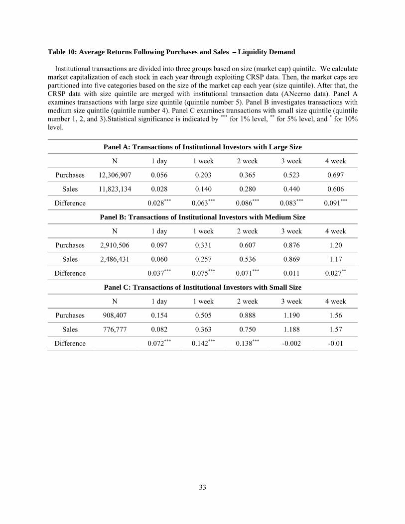
33  

Table 10: Average Returns Following Purchases and Sales – Liquidity Demand Institutional transactions are divided into three groups based on size (market cap) quintile. We calculate market capitalization of each stock in each year through exploiting CRSP data. Then, the market caps are partitioned into five categories based on the size of the market cap each year (size quintile). After that, the CRSP data with size quintile are merged with institutional transaction data (ANcerno data). Panel A examines transactions with large size quintile (quintile number 5). Panel B investigates transactions with medium size quintile (quintile number 4). Panel C examines transactions with small size quintile (quintile number 1, 2, and 3).Statistical significance is indicated by *** for 1% level, ** for 5% level, and * for 10% level.

Panel A: Transactions of Institutional Investors with Large Size

N 1 day 1 week 2 week 3 week 4 week

Purchases 12,306,907 0.056 0.203 0.365 0.523 0.697

Sales 11,823,134 0.028 0.140 0.280 0.440 0.606

Difference 0.028*** 0.063*** 0.086*** 0.083*** 0.091***

Panel B: Transactions of Institutional Investors with Medium Size

N 1 day 1 week 2 week 3 week 4 week

Purchases 2,910,506 0.097 0.331 0.607 0.876 1.20

Sales 2,486,431 0.060 0.257 0.536 0.869 1.17

Difference 0.037*** 0.075*** 0.071*** 0.011 0.027**

Panel C: Transactions of Institutional Investors with Small Size

N 1 day 1 week 2 week 3 week 4 week

Purchases 908,407 0.154 0.505 0.888 1.190 1.56

Sales 776,777 0.082 0.363 0.750 1.188 1.57

Difference 0.072*** 0.142*** 0.138*** -0.002 -0.01

34  

Table 11: Performance of Mutual Funds vs Pension Funds Panel A investigates transactions of money managers, and Panel B examines transactions of pension fund managers. ANcerno data provide a unique identification code for each institution both in cross-section and over time. However, ANcerno data provide an identification code for institution type (money manager and pension sponsor) in only limited period (from July/2009 to September/2011). Therefore, we can identify the institution type for only institutions which made transactions from July/2009 to September/2011. However, since each institution has a unique identification code over time, if the institutions with transactions from July/2009 to September/2011 made transaction in other period, we can identify the institution type for the institutions. Statistical significance is indicated by *** for 1% level, ** for 5% level, and * for 10% level.

Panel A: Transactions of Money Managers

N 1 day 1 week 2 week 3 week 4 week

Purchases 7,328,337 0.051 0.210 0.418 0.625 0.855

Sales 7,119,728 0.043 0.168 0.341 0.567 0.778

Difference 0.008*** 0.042*** 0.077*** 0.057*** 0.077***

Panel B: Transactions of Pension Fund Managers

N 1 day 1 week 2 week 3 week 4 week

Purchases 3,373,137 0.077 0.240 0.413 0.587 0.785

Sales 3,120,262 0.026 0.135 0.328 0.512 0.703

Difference 0.050*** 0.105*** 0.085*** 0.075*** 0.082***

35  

Internet Appendix

On Institutional Trading and Behavioral Bias

36  

Internet Appendix A.1 – Additional Robustness

As a robustness check, we eliminate all transactions of the same stock on a given side (buy versus

sell) within a 20-day period (1-calendar month) ensuring that there is only one institutional transaction in a

given stock on a given side within this window. We do this to remove any instances overlapping returns

of the same stock transacted by either different accounts within a given institutional account, or across

distinct institutions. If there are multiple instances of institutions trading a given stock on a given side we

only keep the earliest such occurrence. In so doing, we create a non-overlapping sample of stock returns

associated with institutional trading on a given side and a given month in order to remove any potential

correlation in stock returns across time and re-estimate the returns over the same time periods. Appendix

Table A.1 reports the results and shows that institutional buys do even better than institutional sells over

the different time horizons.

We also examine if our findings above might be driven by the relatively fewer larger and busier

institutions. We focus our attention on the top 10% (as well as the bottom 90%) – based on trading

frequency as well as trading volume – of the institutional investors. Appendix Table A.2 presents the results

corresponding to the most active institutions in our data where activity is measured by trade frequency. For

comparison, we also present our findings for the remaining 90% of our institutions. We find that neither

the top 10% nor the remaining 90% of institutional investors trade excessively and are therefore not

overconfident by our definition over a time horizon of 1-day, 1-week, 2-weeks, 3-weeks and 1- month. The

average difference between institutional buys and sells for the top 10% of institutional investors who trade

most is 0.016%, 0.047%, 0.073%, 0.056%, and 0.068%, over the trading horizons of 1-day, 1-week, 2-

weeks, 3-weeks, and 1- month, respectively. For the remaining 90% of the institutions in our data, we see

a similar positive difference between buys and sells over the same trading horizons. 30 Thus, not

surprisingly, if we take out the top-decile of the institutions (with highest trading frequency) then the

remaining institutions perform even better.

Different institutions may trade the same stock in overlapping time periods and stock returns are

unlikely to be independent across time. Our bootstrapped results presented in Table 3 should alleviate this

concern.31

Are institutions relatively overconfident traders over periods of economic expansion relative to

periods of economic downturns? It might be reasonable to expect that when stocks are more likely to move

                                                            30 In unreported findings, we estimate similar numbers for institutions classified by trading volume in place of trading frequency. 31 We bootstrap the empirical distribution of the differences in returns for stocks purchased and sold by different institutions in our dataset over the entire sample period. This empirical distribution is generated under the assumption that subsequent returns to stocks bought and sold by the various institutions are drawn from the same underlying distribution. 

37  

upwards than down, as would be the case during periods of economic expansion, that institutions might

display a level of overconfidence which they would not at other times.32 Our macroeconomic cycle results

presents in Table 9 contradict this hypotheses. Institutional buys perform better than the sells during the

contraction cycle and this is predominantly driven by the liquidity motivated sells during economic

downturns.

For our transaction cost calculation, we also use the closing price of that stocks purchased or sold

on the last trading day before the actual trade as the unperturbed price and our results are almost identical.

                                                            32 In an article in the Wall Street Journal in May, 2006, entitled “Behind Surging Stock Market: Old Fashioned Economic Boom,” author E.S. Browning writes: “….Instead, an economic rebound has sent corporate profits to an 11th consecutive quarter of double-digit gains, the longest streak since at least the 1950s. Surprisingly strong growth in the economy and corporate profits has shaken stocks out of their doldrums. The Dow Jones Industrial Average is now within sight of its record close. Unlike the great 1990s bull market, which was sustained by a wave of new technology, this one has the feel of an old-fashioned economic boom, the type investors saw in the 1950s and 1960s. What many thought would be a limited rebound created by Chinese industrial demand has turned into a long-running story as once-unloved sectors such as commodity producers and oil drillers continue to thrive. Helping fuel the U.S. stock surge are once-skeptical investors, who are now funneling money into the market in the hope of getting in on a lengthier boom.”

38  

Internet Appendix A.2 - Supplementary Literature

While theoretical research by Kyle (1985), Glosten and Milgrom (1985), and Easley and O’Hara

(1987) laid the foundation for the impact of trades by informed traders on market depth and the

informativeness of prices, exactly who these informed traders might be has not been specified by this line

of research. That void was filled by Sias and Starks (1997) and Chakravarty (2001), among others, who

provide evidence to support the notion that institutions are smart/informed traders. Intuition suggests that

institutions should not suffer from behavioral biases that have been attributed to individual investors. The

former are expected to act rationally due to their education, training, and better tools at their disposal. Along

those lines, Dhar and Zhu (2006) report that the propensity to sell winners, and the reluctance to sell losers,

is significantly lower for individuals that are wealthier and work in professional occupations.

Daniel, Hirshleifer, and Subrahmanyam (1998) argue that overconfident investors overreact to

private information and underreact to public information.33 They show that such overconfidence driven

trades will, on average, have lower profits because they are exposed to increased volatility as well as

increased trading volume, which increases transaction cost. Gervais and Odean (2001) develop a

multiperiod model of traders learning to become overconfident in the early stages of their career as they

take too much credit for their successes and take appropriate credit for failures. With experience the

overconfidence declines. They also show that overconfident traders trade aggressively, which increases the

expected trading volume as well as volatility.34 , 35 Van den Steen (2011) provides a model in which

Bayesian-rational agents overweight (underweight) information for which they overestimate

(underestimate) the precision, resulting in an overestimation of the precision of the final estimate.

An important intuition from the theoretical literature is that investor overconfidence is developed

over time through a confirmation process of signals. Specifically, in some explicit instances, investors’

private information might be confirmed by how things subsequently emerge in the public domain.

Therefore, if prior private information turns out to be true through revelation of such information in the

                                                            33 De Bondt and Thaler (1985) provide some of the earliest evidence of stock market overreaction to news based on behavioral or psychological bias of the market participants. Using monthly stock data from 1930 to 1975, they show that portfolios of past losers outperform the portfolios of past winners. This suggests an overreaction to news and subsequent adjustment. 34 Kyle and Wang (1997) have argued that overconfident investors generate higher profits than their rational counterparts through more aggressive trading since overconfident investors have a relatively small window within which to obtain, interpret, and act on information signals. Similarly, Benos (1998) argues that overconfident investors could make higher profits than rational traders because they have a first mover advantage through aggressive trading. 35 Odean (1998) develops a methodology to examine investor disposition effects based on gains and losses that are realized versus those on paper and then calculate two metrics on the proportion of gains and losses realized. He finds strong evidence of the disposition effect among retail brokerage clients.  

39  

public domain later, investor confidence is increased. This is another version of the biased self-attribution

leading to overconfidence.

Odean (1999) empirically examines a proprietary sample of individual investor trades and finds

that the profits from stock purchases do not exceed profits from sales even after ignoring trading costs. His

findings support the notion that individual investors overestimate both the precision of information and

their abilities to interpret the same information. In contrast, Statman, Thorley, and Vorkink (STV, 2006)

approach the issue of investor confidence (and, in particular, about investors’ biased self-attribution) from

a macro standpoint by examining the proposition that when investors are overconfident about their

valuation and trading skills we should see relatively high trading volumes. With biased self-attribution,

trading volume should (positively) vary with past market returns. With market level monthly data from

CRSP between 1962 and 2001, STV indeed show that share turnover is positively related to the lagged

market returns for many months. They also show that this positive relationship holds for individual stock

turnover as well which STV interpret as evidence of the disposition effect. Calvet, Campbell, and Sodini

(2009) find strong evidence for disposition effect among Swedish households but less so for mutual funds.

Using retail brokerage data from the US, Ivkovic and Weisbenner (2009) provide contradictory evidence

that individual investors are reluctant to sell funds that have appreciated in value but willing to sell funds

that have lost value. Kumar and Lim (2008) provide evidence that disposition effect is weak among

individual investors when investment decisions are narrowly framed, as measured by clustered trade.

Although Odean (1999) and STV (2006) examine small investors with a retail brokerage account,

researchers have also investigated the link between institutional trading and possible overconfidence but

the results are inconclusive. Grinblatt and Keloharju (2001) find the presence of the disposition effect

among all classes of investors, including individuals and institutions, in the Finnish market. They report

that financial institutions appear to be more willing to liquidate larger losses. Locke and Mann (2005) find

that professional futures traders at the CME hang on to losses significantly longer than gains, thus

displaying disposition effect. Coval and Shumway (2005) provide similar evidence from the CBOT. Using

data from a discount brokerage, Dhar and Zhu (2006) find that wealthier individuals, and those employed

in professional occupations, and frequent traders are less susceptible to display the disposition effect. Using

data from Korean stock index futures Choe and Eom (2009) find that institutions and foreign investors are

less susceptible to disposition effect than individual investors and experienced and sophisticated traders are

also associated with a smaller effect. Barber, Lee, Liu and Odean (2009) find support for the disposition

effect among individuals, corporations, and dealers but not for mutual funds and foreign investors in the

Taiwan Stock Exchange.

Ben-David and Doukas (2006) provide evidence that in presence of ambiguous information

investors become overconfident and trade more frequently even while incurring losses from their trades.

40  

Cremers and Pareek (2011) exploit the short stock holding duration as a proxy for overconfidence and

consistent with the predictions of Daniel, Hirschleifer, and Subrahmanyam (1998), they find that the

presence of short term institutional investors can help explain increases in idiosyncratic volatility because

overconfident investors overreact to private information and underreact to public information.36

Using proprietary data from the United Kingdom and the US, Annaert, Heyman, Vanmaele, and

Van Osselaer (2008) find that mutual fund managers are not overconfident, and are not associated with the

disposition effect. Chuang and Susmel (2011) provide evidence that institutional investors are

overconfident, but less so than individual investors because institutional investors are more informed.

Yung, Sun, and Rahman (2012) find that private information is likely to be associated with high turnover

in stocks with low institutional ownership, consistent with overconfident investor hypothesis. Using

account level data on the TAIFEX from 2001-2006, Chou and Wang (2011) conclude that domestic

institutions display an overconfidence bias but not a disposition bias and individual investors display both

biases.

While these empirical works make important contributions to the literature on behavioral bias

among investors, the evidence on the subject is mixed and many of them (especially those investigating

institutional trading in the US markets) rely on quarterly holdings data. There are obvious problems of

inferring institutional trades from their holdings data as has been effectively argued by Puckett and Yan

(2011). Specifically they point to two important limitations. First, changes in quarterly holdings data do

not capture intra-quarter transactions where funds might purchase and sell or sell and repurchase the same

stock. Second, quarterly holdings do not identify the exact timing or the execution price of the trades.

Specifically, studies with quarterly holdings data typically assume that all trades occur at the end of the

quarter but in reality they could occur at any time within the quarter. Thus researchers employing such data

are severely restricted in their ability to identify superior trading skills if trades are motivated by short term

information and such opportunities dissipate quickly (see also Kothari and Warner (2001)) and likely to

overestimate behavioral biased. By contrast, we use high frequency institutional transactional data that

bypass the problems associated with quarterly data and are well suited to answer transactional level

questions.

                                                            36 They make an additional assumption that institutional investors are more likely to be overconfident than the less experienced individual investors.

41  

Internet Appendix A.3 - Difference between the current work and those of Puckett and Yan (2011) and Chakrabarty, Moulton, and Trzcinka (2017)

The works that most closely resemble ours are by Puckett and Yan (2011) and Chakrabarty, Moulton,

and Trzcinka (2017), henceforth PY and CMT, respectively. In this section, we explain how our work,

specifically, methodology and measurements, sample, results, and conclusions align with or differ from

these two works.

As we have explained in the introduction, the most significant difference between our work and those

of PY and CMT is the method for measuring an institutional manager’s performance. We use fair value

accounting method, which is more likely to track the net asset value (NAV) of a fund, and is more reliable

and value-relevant for financial securities. PY and CMT use historical cost method of calculating security

price change and fund manager performance. Historical cost method requires inventory matching based on

certain assumptions that fair value accounting does not. This major difference in methodology can

contribute to different outcome measurement and conclusions.

PY use buy minus sell performance after adjusting for Daniel, Grinblatt, Titman, and Wermers (1997),

or DGTW adjusted return for the full sample of 3,816 funds from the ANcerno dataset for the sample period

of 1999-2005. Given the difficulty of matching inventory of a specific stock in a portfolio to specific buy

and sell transactions, these authors match sell transactions to the nearest preceding buy transactions (or

last-in-first-out or LIFO method of inventory management) within the quarter, when such transactions

occur, or assume a sell transaction at the end of the quarter. CMT use 1,186 funds present for at least five

or more years in the ANcerno data universe of 4,053 funds for a sample period of 1999-2009 and present

raw and DGTW-adjusted return using first-in-first-out or FIFO method. These authors define short-term

trade as those transactions with a holding period of three months or less.

Our sample period is 1999-2011 and we use raw return from the sample (ANcerno transaction

universe) as well as return from a size- and market-to-book ratio- matched bootstrapped sample (with

replacement) from the CRSP universe. Instead of using either LIFO or FIFO method of inventory matching,

we use the marked-to-marked based fair value method of available for sale financial asset valuation over a

hypothetical holding horizon from 1-day to 4-week. We use this window based on our belief that

information based and short term profit motivated transactions primarily occurs within a short horizon.

Thus, our measure of return is based on a marked-to-market portfolio value used by the futures exchanges

for the purpose of calculating margin balance in a trader’s account. We acknowledge the possibility that

the observed timing or price of the buy or sell transactions may not accurately reflect the time and price the

fund manager intended for the transaction because of execution uncertainty with limit orders and price

uncertainty with market orders.

42  

PY find that institutional investors earn +67 (- 06) basis points DGTW adjusted equally-weighted

return on buy (sell) transactions. Therefore, their equally weighted buy-sell portfolio earns economically

and statistically significant profits after transaction cost. CMT find that institutions earn -0.82% to -3.37%

raw return over a 1-day to 3-month holding period. Thus, these two works differ in their conclusions not

only about the direction of short-term institutional trading performance (profit vs. loss) but also about the

magnitude of the absolute performance.

Our results, obtained using fair value method, are consistent with the findings by CMT that institutions

do not make an economically significant profit on their short term trade, as reported by PY. Our results,

however, do not support the huge short-term underperformance of institutional traders measured by CMT.

We conclude that institutions break-even on their short term trades; they neither make economically

significant profit to infer that that they are skilled at short term trading, nor do they make huge amount of

losses due to agency problem or behavioral bias. We find that institutions earn -16 to +60 basis points on

their buy transactions and -20 to +52 basis points for the sell transactions after transaction cost over 1-day

to 4-week holding period. Thus, institutions earn +3 to +9 basis points more on their short-term buy trades

than their sell trades after transaction cost and these results are vastly different than the estimate of -1.0%

to -5.2% average loss reported by CMT on the short-term trades of institutional investors. Our results for

institutional short-term buy minus sell portfolio returns are in a range that could potentially justify such

trades for a variety of reasons, including liquidity-driven trades. In contrast, it is hard to justify why in

equilibrium the labor market for asset managers would tolerate such large losses as reported by CMT. This

is especially true in light of the conclusion by CMT that the “excessive trading” is due to either the desire

of fund managers to “look active,” which is an agency problem based rational explanation, or “recency

bias,” which is a behavioral bias, of the managers. The first is a contracting problem and the last is a

problem of lack of awareness and education and the effects of both can be attenuated. So why do these

problems continue to exist, and more important, contribute to such large losses?

CMT acknowledge that in the full sample that PY and we use will contain more short-term trades.

They also state that their results are qualitatively similar in the full ANcerno sample than those presented

in their paper and the results are also qualitatively similar when they use holding period of 1-month or less

to define short-term trade. Yet, we expect institutional performance to be worse if we include a higher

proportion of short term trades and redefine short term trades from trades with holding horizon of less than

3-month to less than 1-month.37

                                                            37 They suggest that for most of their analysis their results are similar using either FIFO or LIFO method.

   

43  

For buy trades, our average raw returns in the ANcerno sample and the bootstrapped returns from the

CRSP universe are similar to those in magnitude for the DGTW-adjusted returns reported by PY for the

holding period longer than 1-week but lower for a lower holding-period. The difference in our conclusion

is primarily driven by the sell side of the analysis. In PY, the DGTW-adjusted raw return for the sell side

is -03 to -06 basis points. We find that for a 3-week holding period, which gives us overall results most

similar to the results reported in PY, the buy minus sell portfolio breaks even ( 0 to 8 basis point profit)

rather than making a 34 basis point profit. Yet these differences are not as large as those between the results

of PY and CMT. Unlike the latter, we can’t draw a strong conclusion that the institutions lose money over

short-term trade. Our results suggest significant heterogeneity in raw return for the buy and sell transactions

depending on the different hypothetical holding period ranging from -16 to +60 basis points for buy

transactions and -20 to +52 basis points for the sell transactions over 1-day to 4-week holding period.

A second major difference between PY and CMT is that pension funds perform better than money

managers in the first work and the opposite is true for the latter work. This finding by CMT is surprising

given pension fund managers have longer investment horizon and are subject to less pressure to engage in

liquidity-driven trades due to lower liquidity demand from their clients over shorter horizon. These

conclusions are also inconsistent with the literature that suggests that pension fund managers, and the clients

of pension funds are more sophisticated and use superior performance metrics than mutual funds with retail

and mixed clientele (Guercio and Tkac (2002)). Hence, pension fund managers are more likely to generate

superior performance than mutual funds (Bauer, Cremers, and Frehen (2010)) and are more likely than the

mutual funds to be penalized by clients for poor performance (Guercio and Tkac (2002)).38 We find that

pension funds perform better than money managers over shorter investment horizon and our results are

consistent with PY.

To summarize, our results support neither the conclusions of PY that institutions are skilled at short-

term trading and make a modest profit from these trades after transaction cost, nor those of CMT that short-

term institutional trades are driven by agency problem or behavioral biased and these trades incur huge

losses even before transaction costs. In general, despite methodological differences, our results are closer

in magnitude to those reported by PY than the ones reported by CMT. We do not do any further tests of

persistence of this non-performance “performance.”

Instead, a logical follow-up, and the broader, question we then ask is why institutions trade in the short

term. One of the most frequently used explanations is that the institutions suffer from behavioral biases.

We provide a vector autoregression (VAR) and impulse response based method to directly test for three

                                                            38 Using bias-free data from US pension funds, Bauer, Cremers, and Frehen (2010) report that after expense and trading cost, the abnormal return earned by US pension funds are close to zero or slightly positive, a superior performance than has been reported for mutual funds.  

44  

specific behavioral biases: overconfidence, biased-self-attribution, and disposition effect. We find no

evidence of any of these biases.

Once we have eliminated the common behavioral biases, as a next step, we separate out trades

motivated by alternative rational reasons for trading beyond profit maximization and repeat our analysis.

We conclude that institutions engage in short term trading activities despite earning close to zero net return

after transaction cost for rational reasons such as liquidity, risk management, tax-minimization, or window

dressing. There may be other rational reasons for undertaking these trades such as a desire to cultivate a

stronger relationship with the brokerage houses in order to receive favorable allocation of undervalued

assets such as IPO shares that we have not tested for. Due to data limitation we also cannot test whether

these equity transactions are part of a broader trading strategy, e.g. arbitrage involving futures market or

writing covered call.

CMT also provide robustness checks and/or discuss behavioral biases such as disposition effect or

overconfidence. For overconfidence, they find that funds that have high DGTW-adjusted return in the base

period do not engage in more short-term trades contemporaneously and in the next four semiannual periods

and conclude that institutional investors do not display biased self-attribution driven overconfidence. They

do not test for disposition effect directly but conclude that their results are not consistent with disposition

effect either. CMT rule out these two behavioral biases. They provide evidence that the institutions would

have performed better had they held on to their losses and hence these loss making sales were not to “cut

further losses.” 39 Using these eliminations, they conclude that the motivation for loss making trade could

either be rational, i.e. to “look active,” or behavioral and attributed to a “recency bias”, where individuals

overweight the most recent experiences while making decisions.

Literature suggests that pension fund clients seem not to flock to recent winners and hence pension

fund managers are also less likely to display behavioral biases (Guercio and Tkac (2002)). If pension fund

managers have lower propensity to suffer from behavioral biases, we expect them to perform better than

mutual fund managers. This is what we find while CMT find the opposite. In addition, if institutions

engage in loss making trades to look active, mutual funds are more likely to be under pressure to look active

and perform worse than the pension funds. CMT find the opposite. Our results that pension funds perform

better than mutual funds on short term trades are consistent with the “trading for liquidity” reasons

hypothesis. This is because we expect mutual funds to have more frequent outflow unrelated to fund

performance and due to liquidity (or risk-shifting) need of clients than pension funds and hence the mutual

fund managers are more likely to engage in trades for liquidity reasons. We also observe that during

economic contraction cycle, the underperformance of buy minus sell portfolio is driven almost exclusively

                                                            39 This does not rule out the alternative hypothesis that the capital that was freed up from the loss-making transactions might have performed better on a different (unobserved) investment choice relative to the “do nothing alternative.”

45  

by the sell transactions. As investors demand liquidity perhaps to finance consumption or for risk-shifting

reasons during such periods, this is another evidence of liquidity-driven trade hypothesis.

In summary, although some of our basic results fall within the very wide spectrum of those

contradictory results reported in PY and CMT, due to the difference in magnitude, our conclusions on short-

term trading performance differ from both these works. Although some of our conclusions on behavioral

bias, or lack thereof, for institutional traders may be similar to those in CMT, we provide direct and more

systematic tests for all the behavioral biases that we reject. We conclude that institutions engage in short

term trading activities despite earning close to zero net return, after transaction cost, for rational reasons

such as liquidity, risk management, tax-minimization, or window dressing. Although our results suggest

that managers engaging in short-term trading are likely to earn zero net return or even lose a few basis

points from these trades, for the vast majority of the cases – except for window dressing – those trades are

in response to real constraints or frictions and welfare implications of these trades are minimal. Thus, our

results and conclusions can survive the equilibrium argument.

46  

Reference: Annaert, J., Heyman, D., Vanmaele, M., Van Osselaer, S., 2008. Disposition bias and overconfidence in

institutional trades. Working Paper, Belgium. Bauer, R., Cremers, M., and Frehen, R., 2010, Pension Fund Performance and Costs: Small is Beautiful,

working paper, Tilburg University. Benos, A.V., 1998. Aggressiveness and survival of overconfident traders. Journal of Financial Markets 1,

353-383. Calvet, L. E., Campbell, J.Y., Sodini, P., 2009. Fight or flight? Portfolio rebalancing by individual investors,

Quarterly Journal of Economics, 124, 301-348. Choe, H., and Eom, Y., 2009. The disposition effect and investment performance in the futures market,

Journal of Futures Markets, 29, 496-522. Chou, R.K., Wang, Y.Y., 2011. A test of the different implications of the overconfidence and disposition

hypotheses. Journal of Banking & Finance 35, 2037-2046. Chuang, W., and Susmel, R., 2011. Who is the more overconfident trader? Individual vs. institutional

investors, Journal of Banking and Finance, 35, 1626-1644. Coval, J.D., Shumway, T., 2005. Do behavioral biases affect prices? Journal of Finance, 60, 1-34. Dhar, R., Zhu, N., 2006. Up close and personal: An individual level analysis of the disposition effect,

Management Science 52, 726-740. Easley, D., O'hara, M., 1987. Price, trade size, and information in securities markets. Journal of Financial

Economics 19, 69-90. Glosten, L.R., Milgrom, P.R., 1985. Bid, ask and transaction prices in a specialist market with

heterogeneously informed traders. Journal of financial economics 14, 71-100. Ivković, Z. and Weisbenner, S., 2009, Individual investor mutual fund flows, Journal of Financial

Economics 92, 223-237 Kothari, S. P., Warner, J.B., 2001. Evaluating mutual fund performance. Journal of Finance, 56, 1985-

2010. Kumar, A., and Lim, A.S., 2008, How Do Decision Frames Influence the Stock Investment Choice of

Individual Investors, Management Science, 54, 1052-1064. Kyle, A.S., 1985. Continuous Auctions and Insider Trading. Econometrica, 53, 1315-1335. Kyle, A.S., Wang, F.A., 1997. Speculation duopoly with agreement to disagree: can overconfidence survive

the market test? Journal of Finance 52, 2073-2090. Locke, P.R., Mann, S.C., 2005. Professional trader discipline and trade disposition. Journal of Financial

Economics 76, 401-444. Van den Steen, E., 2011, Overconfidence by Bayesian-Rational Agents, Management Science, 57, 884-896. Yung, K., Sun, Q., Rahman, H., 2012. Trading volume and overconfidence with differential information,

and heterogeneous investors. Journal of Behavioral Studies in Business 5, 1-31.

47  

Internet Appendix Table A.1: Average Returns Following Purchases and Sales - after Removing Overlapping Returns We create a subsample of institutional buys and sells such that there is only one (the earliest) instance of an institutional transaction of a given stock on a given side (buy or sell) in a 20 day period (1 calendar month). Average returns to stocks bought (sold) by institutional investors over the various time horizons is:

R ,∑ ∏ 1 ,

1

where N is number of buying (selling) transactions, T is institutional holding period (time horizons of trading days subsequent to buying (selling) transactions, and , is CRSP daily return for stock j corresponding to institutional transaction i on day r after transaction day t. In order to calculate the return using ANcerno data, we initially construct the integrated daily stock level institutional data through the data integration process. This process allows our data to match with CRSP daily return for cumulative return , ). Using CRSP return, we calculate the cumulative returns to stocks bought (sold) by institutional investors over various horizons of trading days (∏ 1 , . Then, we calculate the average returns to the stocks bought (sold). Statistical significance is indicated by *** for 1% level, ** for 5% level, and * for 10% level.

Transactions of Institutional Investors with One Month Interval

N 1 day 1 week 2 week 3 week 4 week

Purchases 2,804,835 0.062 0.147 0.301 0.489 0.758

Sales 2,908,818 0.005 0.058 0.183 0.367 0.598

Difference 0.057*** 0.089*** 0.117*** 0.121*** 0.160***

48  

Internet Appendix Table A.2: Average Returns Following Purchases and Sales Based on Trade Frequency and Trading Volume Panel A investigates the transactions made by the top 10% of the institutional investors in the sample who make the greatest number of trades. Panel B examines the transactions conducted by the remaining 90% of the institutional investors in the sample who trade least. Statistical significance is indicated by *** for 1% level, ** for 5% level, and * for 10% level.

Panel A: The 10 Percent of Institutional Investors Who Trade Most Frequently

N 1 day 1 week 2 week 3 week 4 week

Purchases 12,092,406 0.061 0.231 0.435 0.626 0.842

Sales 11,022,952 0.046 0.184 0.361 0.570 0.774

Difference 0.016*** 0.047*** 0.073*** 0.056*** 0.068***

Panel B: The 90 Percent of Institutional Investors Who Trade Least Frequently

N 1 day 1 week 2 week 3 week 4 week

Purchases 4,033,414 0.092 0.280 0.450 0.621 0.820

Sales 4,063,390 0.010 0.135 0.306 0.493 0.681

Difference 0.082*** 0.145*** 0.144*** 0.128*** 0.139***