arX

iv:0

711.

3280

v2 [

astr

o-ph

] 2

6 M

ar 2

008

Chaotic behavior in the accretion disk

LIU Lei∗ and HU Fei

Institute of Atmospheric Physics, Chinese Academy of Sciences, Beijing 100029, China

(Dated: February 6, 2020)

Abstract

The eccentric luminosity variation of quasars is still a mystery. Analytic results of this behavior

ranged from multi-periodic behavior to a purely random process. Recently, we have used nonlinear

time-series analysis to analyze the light curve of 3C 273 and found its eccentric behavior may

be chaos [L. Liu, Chin. J. Astron. Astrophys. 6, 663 (2006)]. This result induces us to look

for some nonlinear mechanism to explain the eccentric luminosity variation. In this paper, we

propose a simple non-linear accretion disk model and find it shows a kind of chaotic behavior

under some circumstances. Then we compute the outburst energy △F , defined as the difference of

the maximum luminosity and the minimum luminosity, and the mean luminosity 〈F 〉. We find that

△F ∼ 〈F 〉α in the chaotic domain, where α ≈ 1. In this domain, we also find that 〈F 〉 ∼ M0.5,

where M is the mass of central black hole. These results are confirmed by or compatible with some

results from the observational data analysis [A. J. Pica and A. G. Smith, Astrophys. J. 272, 11

(1983); M. Wold, M. S. Brotherton and Z. Shang, Mon. Not. R. Astron. Soc. 375, 989 (2007)].

PACS numbers: 98.54.Aj, 98.62.Mw, 05.45.-a

∗Electronic address: liulei@mail.iap.ac.cn; Also at Graduate University of the Chinese Academy of Sciences,

Beijing 100049, China

1

I. INTRODUCTION

Since the discovery of quasar in 1963 [1], the luminosity variation has played an important

role in our understanding of its nature. Although it has been subjected to extensive analysis,

there is no generally accepted method of extracting the information in the light curve.

Results of analysis of the light curve ranged from multi-periodic behavior [2, 3, 4, 5] to

a purely random process [6, 7, 8]. On the basis of these analysis, many theories which

ranged from periodic mechanisms [5, 9, 10] to superimposed random events such as the so-

called Christmas tree model [11], have been proposed. Then whatever does this seemingly

random light curve tell us? Could this seeming randomness be some behavior other than

multi-periodic or purely random?

Also in 1963, Edward Lorenz published his monumental work entitled Deterministic Non-

periodic Flow [12]. In this paper, he found a strange behavior which can appear in a de-

terministic non-linear dissipative system, which seems random and unpredictable, and is

called Chaos. Chaotic behavior is not multi-periodic because it has a continuous spectrum.

Useful information can not always be extracted from the power spectrum of chaotic sig-

nal. On the other hand chaotic behavior is not random either because it can appear in a

completely deterministic system. The concept of attractor is often used when describing

chaotic behaviors. As the dissipative system evolves in time, the trajectory in state space

may head for some final region called attractor. The attractor may be an ordinary Euclidean

object or a fractal [13] which has a non-integer dimension and often appears in the state

space of a chaotic system. For many practical systems, we may not know in advance the

required degrees of freedom and hence can not measure all the dynamic variables. How can

we discern the nature of the attractor from the available experimental data? Packard et al.

[14] introduced a technique which can be used to reconstruct state-space attractor from the

time series data of a single dynamical variable. Moreover, the correlation integral algorithm

subsequently introduced by Grassberger and Procaccia [15] can be used to determine the

dimension of the attractor embedded in the new state space. These techniques constitute a

useful diagnostic method of chaos in practical systems.

Therefore, the above-mentioned diagnostic methods have been used to analyze the light

curve of 3C 273, and it has been found that the eccentric luminosity variation of 3C 273

may be a kind of chaotic behavior [16]. This result tells us that non-linear may play a

2

very important role in the nature of quasar. Then whatever role does the non-linear play?

Could the non-linear mechanisms help us understand the eccentric behavior in the luminosity

variation of quasars?

For the sake of keys, we in this paper propose a simple non-linear accretion disk (NAD)

model, by borrowing basic ideas from the standard accretion disk (SAD) [17, 18]. We then

find that with some parameters the disk shows a kind of chaotic behavior. Although our

model is based on the SAD, there are two main differences between them. First, SAD is

a stable disk which can not be used to explain the eccentric luminosity variation. Second,

SAD uses the complex differential equations of fluid dynamics to describe its evolution and

NAD uses iterated equations. The latter simplifies the problem to a great degree. In the

following sections, you will see very simple non-linear terms can produce extremely complex

light curves. What’s more, NAD is more natural than many other models on luminosity

variation because our world is a non-linear world and the NAD aims to explore the non-

linear effects on the quasar. Overall, our results provide a new view of the nature of the

eccentric luminosity variation and may be helpful in the future study of quasars.

II. DESCRIPTION OF THE CHAOTIC ACCRETION DISK MODEL

There are always two kinds of factors which can be classified by their contrary contribu-

tions to the behavior of the non-linear chaotic systems. For example, in the famous Logistic

model [19], one factor is related with the plenty food and/or space etc., and the other is

related with the overpopulation and disease. The formal can make the population grow, and

the latter can make the population decrease. The interaction of the two factors can lead

to the chaotic variation of the population under some circumstances. The other example

is the Lorenz model [12]. In this model, the two kinds of contrary factors are the heating

of the earth, and the viscous stresses and the gravity. The heating of the earth can make

the air rise. However the viscous stresses and the gravity always prevent the air rising. The

interaction between them will lead to the chaotic behavior of the air.

We note that the standard accretion disk (SAD) also has two kinds of contrary factors

as in the above models. On the one hand, the viscous stresses will make the gas rotate

slowly around the black hole. On the other hand, the gas in the disk will flow towards black

hole, for its centrifugal force and gravity is not in equilibrium due to viscous stresses. The

3

gravitational potential energy will convert to the kinetic energy on the process of flowing

towards the black hole which makes the gas rotate fast. Thus the viscous stresses and the

gravity are the two contrary factors in the SAD. This is the start point of our non-linear

accretion disk (NAD) model. By borrowing these basic ideas, we now construct the NAD

model as follows.

We consider an accretion disk which has only two layers of gas, as in Fig. 1. It is supposed

that (a) the thickness of each layer is very small that the tangential velocity in each layer

is slightly different from its average tangential velocity. That is to say, we only need one

velocity to describe the circular motion of one layer; (b) the height of disk H is very small

that the motion is almost two-dimensional; (c) the average tangential velocity of outer layer

is a constant and equals its average Kepler’s velocity V . Due to the viscous stresses, the

average tangential velocity of inner layer u does not equal its average Kepler’s velocity U ,

and is a time variable; (d) the inner layer interacts with outer layer by viscous stresses, but

it does not interact with black hole; (e) during small interval △τ , the mass △m flows across

any circle (all the centers of circles are on the center of black hole) is the same. If U2 > u2,

the centrifugal force is less than the gravity and the gas will flow towards black hole. Define

△m > 0 in such a case. If U2 < u2, the gas will flow far from the black hole and △m < 0.

When U2 = u2, △m = 0. Thus, we simply suppose that △m ∝ U2 − u2; (f) there is a

boundary layer between outer layer and inner layer. The thickness of this boundary layer

h is very small comparing with the radius r of the inner layer’s outer edge. When gas in

the outer layer flows across the boundary layer, the average tangential velocity will change

from V to U ; (g) Any relativistic effect is not considered here. All above are the basic

assumptions of our NAD model.By these assumptions, the equations of motion are derived

as follows.

At the nth moment, the viscous stresses acting on the inner layer is,

fn = 2πrHµun − V

h,

where un is the average tangential velocity of inner layer at the nth moment and µ is the

viscosity. Then we have,

2πrHµun − V

h= m

un − un+1−

△τ,

where m is the mass of inner layer, un+1− is the average tangential velocity of inner layer at

(n + 1)th moment due to the action of viscous stresses, and △τ is the time interval between

4

u

V

r △m △m △m

FIG. 1: The NAD model. The black dot at the centre of this figure represents a black hole and the

shadow region is the boundary layer. Broad arrays represent the flow of mass towards black hole.

nth and (n + 1)th moments. Thus it can be obtained that,

un+1− = un −

2πrHµ△τ

hm(un − V ). (1)

When un2 < U2, the mass △mn in inner layer will flow into black hole, which causes

the same mass to flow across boundary layer into inner layer. When the gas flows across

boundary layer, its velocity will change from V to U . According to the assumption (e),

△mn

m= C

(

1−un

2

U2

)

(2)

where C is a dimensionless parameter. At the (n + 1)th moment, the average tangential

velocity due to the flow of mass towards black hole is

un+1+ =

(m−△mn)un +△mnU

m= un + (U − un)

△mn

m.

According to Eq. (2), we have

un+1+ = un + C

(

1−un

2

U2

)

(U − un). (3)

When un2 > U2, there is only mass flowing out of inner layer, which will not change the

average tangential velocity of inner layer. Thus,

un+1+ = un. (4)

Finally, the average tangential velocity of inner layer at the (n + 1)th moment is

un+1 = un+1+ + un+1

− − un.

5

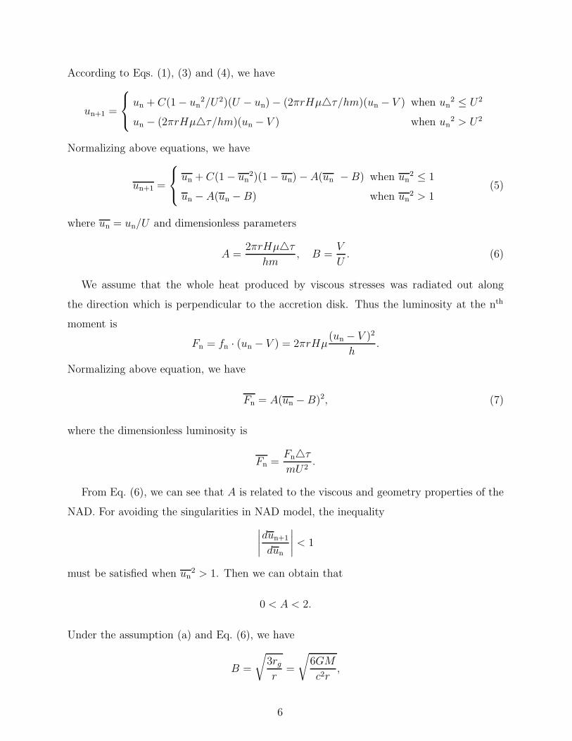
According to Eqs. (1), (3) and (4), we have

un+1 =

un + C(1− un2/U2)(U − un)− (2πrHµ△τ/hm)(un − V ) when un

2 ≤ U2

un − (2πrHµ△τ/hm)(un − V ) when un2 > U2

Normalizing above equations, we have

un+1 =

un + C(1− un2)(1− un)−A(un −B) when un

2 ≤ 1

un − A(un − B) when un2 > 1

(5)

where un = un/U and dimensionless parameters

A =2πrHµ△τ

hm, B =

V

U. (6)

We assume that the whole heat produced by viscous stresses was radiated out along

the direction which is perpendicular to the accretion disk. Thus the luminosity at the nth

moment is

Fn = fn · (un − V ) = 2πrHµ(un − V )2

h.

Normalizing above equation, we have

Fn = A(un − B)2, (7)

where the dimensionless luminosity is

Fn =Fn△τ

mU2.

From Eq. (6), we can see that A is related to the viscous and geometry properties of the

NAD. For avoiding the singularities in NAD model, the inequality

∣

∣

∣

∣

dun+1

dun

∣

∣

∣

∣

< 1

must be satisfied when un2 > 1. Then we can obtain that

0 < A < 2.

Under the assumption (a) and Eq. (6), we have

B =

√

3rgr

=

√

6GM

c2r,

6

where rg is the Schwarzschild radius, c is the velocity of light and M is the mass of the black

hole. Clearly, B is related to the mass of the black hole and the geometry properties of the

NAD and

0 < B < 1.

The parameter C can also be related to some physical quantities. The distance that the

mass △m at the outer edge of inner layer travels towards black hole during △τ is,

△s =U2 − u2

2r△τ 2.

Then we can be obtained that

△m

m=

πρHU2△τ 2

m(1− u2). (8)

Comparing Eqs. (8) with (2), we find that

C =πρHU2△τ 2

m=

U2△τ 2

r2=

c2△τ 2

6r2.

We can see that C is only related to the geometry properties of the NAD. Here we assume

that the mass of inflow or outflow during △t do not exceed the mass of the inner layer, that

is,

− 1 <△mn

m< 1. (9)

For the inequality △mn/m < 1 is always satisfied when un2 ≤ 1, we choose

0 < C < 1

in the following discussion. From above discussions, we can see that only A is related to the

viscous property of NAD, and only B is related to the mass of black hole. Thus by tuning

corresponding parameter, we can easily know the effect of the variation of some physical

property on the behavior of the NAD and its light curve. Some results are given in the

following sections.

III. RESULTS

In this section, some properties of our model will be discussed by numerical computation.

First,we will discuss the long-term chaotic behavior of NAD with different viscous properties.

7

0.8 1.0 1.2 1.4 1.6 1.8 2.0

-1.0

-0.5

0.0

0.5

1.0

u

/ U

A

(a)

0.8 1.0 1.2 1.4 1.6 1.8 2.0

0

1

2

3

F /

mU

2

A

(b)

1000 1020 1040 1060 1080 1100-0.4

-0.3

-0.2

-0.1

0.0

0.1

0.2

0.3

0.4

u n / U

n

(c)

1000 1020 1040 1060 1080 11001.0

1.2

1.4

1.6

1.8

2.0

2.2

2.4

2.6

2.8

3.0

F n /

mU

2

n

(d)

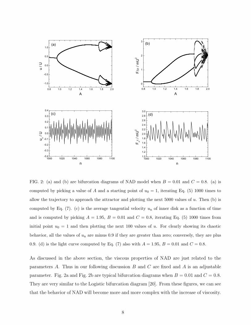
FIG. 2: (a) and (b) are bifurcation diagrams of NAD model when B = 0.01 and C = 0.8. (a) is

computed by picking a value of A and a starting point of u0 = 1, iterating Eq. (5) 1000 times to

allow the trajectory to approach the attractor and plotting the next 5000 values of u. Then (b) is

computed by Eq. (7). (c) is the average tangential velocity un of inner disk as a function of time

and is computed by picking A = 1.95, B = 0.01 and C = 0.8, iterating Eq. (5) 1000 times from

initial point u0 = 1 and then plotting the next 100 values of u. For clearly showing its chaotic

behavior, all the values of un are minus 0.9 if they are greater than zero; conversely, they are plus

0.9. (d) is the light curve computed by Eq. (7) also with A = 1.95, B = 0.01 and C = 0.8.

As discussed in the above section, the viscous properties of NAD are just related to the

parameters A. Thus in our following discussion B and C are fixed and A is an adjustable

parameter. Fig. 2a and Fig. 2b are typical bifurcation diagrams when B = 0.01 and C = 0.8.

They are very similar to the Logistic bifurcation diagram [20]. From these figures, we can see

that the behavior of NAD will become more and more complex with the increase of viscosity.

8

-2.0 -1.6 -1.2 -0.8 -0.4 0.0

-1.2

-0.8

-0.4

0.0

D=0.88639+/-0.00293

Log 10

Cor

(R)

Log10R

correlation integral of un

(e)

-2.0 -1.6 -1.2 -0.8 -0.4 0.0

-1.5

-1.0

-0.5

0.0

D=0.96886+/-6.0365E-4

Log 10

Cor

(R)

Log10R

correlation integral of Fn

(f)

FIG. 3: (e) and (f) are correlation integrals when A = 1.95, B = 0.01 and C = 0.8. They are

computed by using 5000 data after 1000 iterations as in Fig. 2(a)–(d), and the corresponding

correlation dimension is given in each plot.

Specially, there is a piece of vague area on the right side of each figure. The behavior of u in

Fig. 2a (or F in Fig. 2b) in this area will be chaotic. Fig. 2c is the evolution of the average

tangential velocity u of the inner layer and Fig. 2d is the light curve generated by NAD

model. Both of them are plotted when A = 1.95,B = 0.01,C = 0.8, with which the system

shows a kind of chaotic behavior. Here we must note that the choice of the parameters is

not arbitrary. Any choice of the parameters should guarantee that Eq. (9) must be satisfied.

By many numerical computations, we find that when A is greater than about 1.9 and C is

greater than about 0.6, Eq. (9) is satisfied and the luminosity is chaotic.

The correlation integral [15] is also used to analyze our model. Let X1, X2, . . . , XN be

samples of a physical variable (u or F in our model) at the ith moment, i = 1, 2, . . . ,N. The

correlation integral is defined as

Cor(R) =1

N(N− 1)

N∑

i=1

N∑

j=1,j 6=i

θ(R− |Xi −Xj|),

where θ(x) is the Heaviside function,

θ(x) =

1 x ≥ 0

0 x < 0.

In Ref. 15, they have studied many chaos models and found that

Cor(R) ∝ RD,

9

0.7 0.8 0.9 1 1.1 1.2 1.3−1.4

−1.2

−1

−0.8

−0.6

−0.4

−0.2

0

0.2

0.4

Log ⟨ F ⟩

Log

∆ F

FIG. 4: The outburst energy △F as a function of the mean luminosity Fm. Here, we choose four

groups of parameters. In each group, parameters A and C are fixed, whereas B varies in the interval

(0, 1), so long as the light curve is chaotic and Eq. (9) is satisfied. The samples of the light curve are

produced as in Fig. 2 and the results are plot with lines and different symbols. The corresponding

parameters and the slope of the line α are given as follows. Point, A = 1.95, C = 0.8, α ≈ 0.93; cross,

A = 1.97, C = 0.8, α ≈ 0.96; plus, A = 1.98, C = 0.8, α ≈ 0.97; star, A = 1.98, C = 0.6, α ≈ 0.97.

where D is called correlation dimension. Strictly D is not the dimension of the attractor,

but is very close to it. According to chaos and non-linear dynamics, if an attractor for a

dissipative system has a non-integer dimension, then the attractor is a chaotic attractor [20].

Therefore, the correlation integral is a useful diagnostic tool of chaos. However, itself does

not have any physical meaning. Fig. 3e and Fig. 3f are typical results of correlation integral

when A = 1.95, B = 0.01, C = 0.8. From these results, we can see that attractors in the

state space of u and F are indeed chaotic attractors.

We then discuss the relationship of the outburst energy and the mean luminosity. The

outburst energy △F is defined as the difference between maximum luminosity F (max) and

minimum luminosity F (min), that is,

△F = F (max)− F (min).

This definition is the same as in Ref. 21. Here, we fix the parameters A and C and compute

the luminosity with different B. For a guarantee of satisfying Eq. (9) and the chaotic

10

0 0.05 0.1 0.15 0.2 0.25 0.3 0.352

2.2

2.4

2.6

2.8

3

3.2

3.4

3.6

B

⟨ F ⟩

FIG. 5: The mean luminosity as a function of the parameter B. The parameters, the samples of

the light curve and the corresponding symbols are the same as Fig. 4. The line in the plot is

〈F 〉 = 4.3B + 2.

behavior in the light curve, we choose A > 1.9 and C > 0.6, as was stated above. Then we

compute the outburst energy and and the mean luminosity 〈F 〉, and find that

△F ∼ 〈F 〉α, (10)

where α ≈ 1, as in Fig. 4. This result is very similar with the observational facts found in

the Fig. 7 of Ref. 21, where they found that for most sources it appears that the outburst

energy scales with the mean luminosity. Additionally, we should note that B is related to

the mass of the black hole. Thus this find suggests that the mass of black hole may not

affect the nature of the properties of the luminosity variation. Quasars with big black holes

will obey the same rules of the luminosity variation as the small ones. By fixing A and C,

the relationship of mean luminosity and the mass of black hole is also discussed. We find

that the mean luminosity scales with B, as in Fig. 5. With Eq. (6), we can conclude that,

〈F 〉 ∼ M1/2. (11)

Combining Eq.(10) with Eq. (11), we immediately obtain that,

△F ∼ Mβ , (12)

11

where β ≈ 1/2. Ref. 22 have reported that it is evident that the sources displaying largest

variability amplitudes have, on average, higher black hole masses, although there is no linear

relationship between them. Eq. (12) is compatible with their results.

IV. DISCUSSION AND CONCLUSION

In this paper we propose a non-linear accretion disk model (NAD) which can be used to

describe the chaotic behavior observed in the light curve of quasar 3C 273 [16]. We note

that the tangential velocity of accretion disk is influenced by two factors. One is the viscous

stresses and the other is the flow of mass towards black hole. Under some circumstances, one

of them may reduce the velocity and the other may increase it. Because of non-linear, the

winner of gaining upper hand among them always vary with time. Then a kind of irregular

oscillation of accretion disk would come out. It finally leads to the chaotic luminosity

variation.

Although any complex multi-periodic mechanism and unnatural random event is not

included, very simple non-linear terms in our model can also produce extremely complex

behavior of the accretion disk. Meanwhile, for understanding the underlying non-linear na-

ture of the chaotic behavior of the light curve, we ignore many physical details, including

some may be very important to the behavior of the quasars. For example, the effects of

the thermodynamics [23], the interaction between the inner edge of the inner layer and the

black hole [24], and the details of the dynamics happening in the boundary layer are not

considered here. Additionally, we use the iterated equations instead of the complex equa-

tions of fluid dynamics. All above-mentioned facts simplify the problem greatly. However,

the simplification does not weaken the validity of our model on explaining the eccentric

luminosity variation. The model can shows two rules in the chaotic domain. One is the

outburst energy △F ∼ 〈F 〉α, where 〈F 〉 is the mean luminosity and α ≈ 1; the other is

〈F 〉 ∼ M0.5, where M is the mass of central black hole. There rules are confirmed by or

compatible with the observational data analysis [21, 22].

The standard accretion disk model (SAD) is always be recognized as a standard picture

of the AGNs, for it can produce extreme energy that be observed in the AGNs [25]. Our

NAD model just borrows the basic idea of the SAD. Thus, we conclude that the chaotic

behavior presenting in NAD model can be seen in many eccentric light curves of the AGNs.

12

Some authors have reported that other AGNs may have chaotic behavior in their eccentric

light curves [26]. However, we hope that there will be more evidences to support or oppose

the assertions of our model, especially the quantitative rules predicted in this paper.

Overall, our results reveal that the non-linear plays a key role in the cause of the eccen-

tric luminosity variation of quasars. The omnipresent non-linear is very important in our

understanding of this complex world, as chaos and non-linear dynamics tells us. Thus it is

nature to study the luminosity variation of quasars from the view of non-linear. And we

hope chaos and non-linear dynamics may be helpful in the further study of quasars.

Acknowledgments

LIU Lei thanks Professor Meng Ta-Chung for his kind help to understand the chaos and

non-linear dynamics. Many thanks go to Dr. CHENG Xue-Ling, GUO Long, ZHU Li-Lin

and DING Heng-Tong for helpful discussions and ZHU Yan for improving the plot. This

research is supported by the National Nature Science Foundation of China under Grant No.

40405004.

13

[1] H. J. Smith and D. Hoffleit, Nature 198, 650 (1963).

[2] W. E. Kunkel, Astron. J. 72, 1341 (1967).

[3] I. Jurkevich, Astrophys. Space Sci. 13, 154 (1971).

[4] A. Sillanpaa, S. Haarala, and T. Korhonen, Astron. Astrophys. Suppl. Ser. 72, 347 (1988).

[5] R. G. Lin, Chin. J. Astron. Astrophys. 1, 245 (2001).

[6] T. Manwell and M. Simon, Astron. J. 73, 407 (1968).

[7] J. Terrell and K. H. Olsen, Astrophys. J. 161, 399 (1970).

[8] G. G. Fahlman and T. J. Ulrych, Astrophys. J. 201, 277 (1975).

[9] Z. Abraham and G. E. Romero, Astron. Astrophys. 344, 61 (1999).

[10] G. E. Romero et al., Astron. Astrophys. 360, 57 (1999).

[11] R. L. Moore et al., Astrophys. J. 260, 415 (1982).

[12] E. N. Lorenz, J. Atmos. Sci. 20, 130 (1963).

[13] J. Feder, Fractal (Plenum, New York, 1988).

[14] N. H. Packard, J. P. Crutchfield, and J. D. Farmer, Phys. Rev. Lett. 45, 712 (1980).

[15] P. Grassberger and I. Procaccia, Phys. Rev. Lett. 50, 346 (1983).

[16] L. Liu, Chin. J. Astron. Astrophys. 6, 663 (2006).

[17] N. I. Shakura and R. A. Sunyaev, Astron. Astronphys. 24, 337 (1973).

[18] J. E. Pringle, Ann. Rev. Astron. Astrophys. 19, 137 (1981).

[19] R. M. May, Nature 261, 459 (1976).

[20] R. C. Hilborn, Chaos and Nonlinear Dynamics (Oxford Univ. Press, Oxford, 1994).

[21] A. J. Pica and A. G. Smith, Astrophys. J. 272, 11 (1983).

[22] M. Wold, M. S. Brotherton, and Z. Shang, Mon. Not. R. Astron. Soc. 375, 989 (2007).

[23] R. Narayan and I. Yi, Astrophys. J. 428, L13 (1994).

[24] J. H. Krolik and J. F. Hawley, Astrophys. J. 573, 754 (2002).

[25] D. Lynden-Bell, Nature 223, 690 (1969).

[26] R. Misra et al., Astrophys. J. 643, 1134 (2006).

14