Embed Size (px)
Citation preview
A single proportionMultiple proportions
Analyzing Proportions
Maarten L. Buis
Institut für SoziologieEberhard Karls Universität Tübingen
www.maartenbuis.nl
Maarten L. Buis Analyzing Proportions
A single proportionMultiple proportions
The problem
I A proportion is bounded between 0 and 1,
this means that:I the effect of explanatory variables tends to be non-linear,
andI the variance tends to decrease when the mean gets closer
to one of the boundaries.I This makes linear regression unattractive.
Maarten L. Buis Analyzing Proportions
A single proportionMultiple proportions
The problem
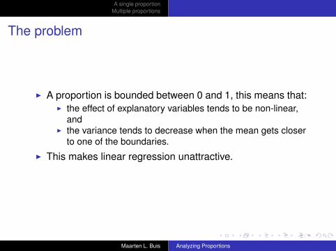
I A proportion is bounded between 0 and 1, this means that:
I the effect of explanatory variables tends to be non-linear,and
I the variance tends to decrease when the mean gets closerto one of the boundaries.
I This makes linear regression unattractive.
Maarten L. Buis Analyzing Proportions
A single proportionMultiple proportions
The problem
I A proportion is bounded between 0 and 1, this means that:I the effect of explanatory variables tends to be non-linear,
and
I the variance tends to decrease when the mean gets closerto one of the boundaries.
I This makes linear regression unattractive.
Maarten L. Buis Analyzing Proportions
A single proportionMultiple proportions
The problem
I A proportion is bounded between 0 and 1, this means that:I the effect of explanatory variables tends to be non-linear,
andI the variance tends to decrease when the mean gets closer
to one of the boundaries.
I This makes linear regression unattractive.
Maarten L. Buis Analyzing Proportions
A single proportionMultiple proportions
The problem
I A proportion is bounded between 0 and 1, this means that:I the effect of explanatory variables tends to be non-linear,
andI the variance tends to decrease when the mean gets closer
to one of the boundaries.I This makes linear regression unattractive.
Maarten L. Buis Analyzing Proportions
A single proportionMultiple proportions
Solutions
I model the distribution of the dependent variable(s) witheither
I a beta distribution, betafitI a zero/one inflated beta distribution, zoibI a Dirichlet distribution, dirifit
I model how the mean proportion relates to explanatoryvariables using
I a fractional logit, glmI a fractional multinomial logit, fmlogit
Maarten L. Buis Analyzing Proportions
A single proportionMultiple proportions
Solutions
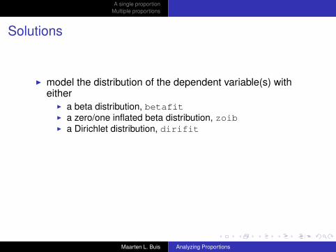
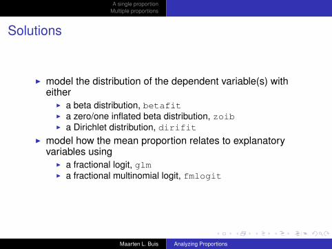
I model the distribution of the dependent variable(s) witheither
I a beta distribution, betafitI a zero/one inflated beta distribution, zoibI a Dirichlet distribution, dirifit
I model how the mean proportion relates to explanatoryvariables using
I a fractional logit, glmI a fractional multinomial logit, fmlogit
Maarten L. Buis Analyzing Proportions
A single proportionMultiple proportions
Outline
A single proportion
Multiple proportions
Maarten L. Buis Analyzing Proportions
A single proportionMultiple proportions
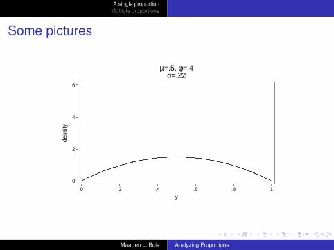
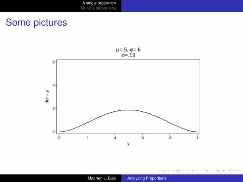
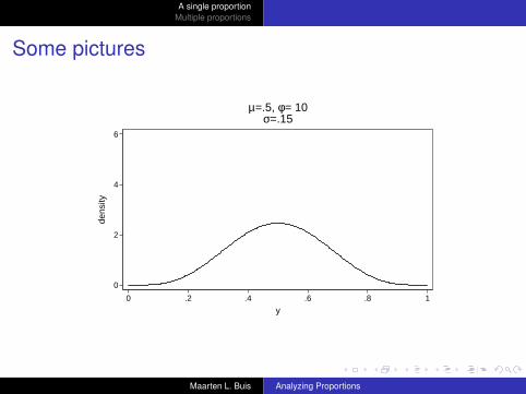
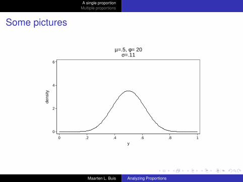
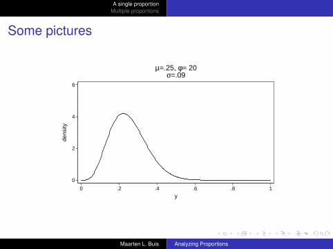
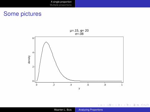
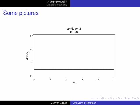
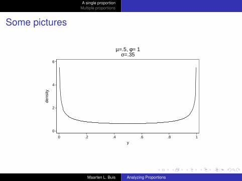
the beta distribution
I A flexible distribution bounded between 0 and 1 (excluding0 and 1)
I Two parameters: the mean and a scale parameter.I The variance is a function of the mean and the scale
parameter: the variance is largest when the mean is 0.5.
Maarten L. Buis Analyzing Proportions
A single proportionMultiple proportions
the beta distribution
I A flexible distribution bounded between 0 and 1 (excluding0 and 1)
I Two parameters: the mean and a scale parameter.
I The variance is a function of the mean and the scaleparameter: the variance is largest when the mean is 0.5.
Maarten L. Buis Analyzing Proportions
A single proportionMultiple proportions
the beta distribution
I A flexible distribution bounded between 0 and 1 (excluding0 and 1)
I Two parameters: the mean and a scale parameter.I The variance is a function of the mean and the scale
parameter:
the variance is largest when the mean is 0.5.
Maarten L. Buis Analyzing Proportions
A single proportionMultiple proportions
the beta distribution
I A flexible distribution bounded between 0 and 1 (excluding0 and 1)
I Two parameters: the mean and a scale parameter.I The variance is a function of the mean and the scale
parameter: the variance is largest when the mean is 0.5.
Maarten L. Buis Analyzing Proportions
A single proportionMultiple proportions
Some pictures
0
2
4
6
dens
ity
0 .2 .4 .6 .8 1
y
µ=.5, φ= 4σ=.22
Maarten L. Buis Analyzing Proportions
A single proportionMultiple proportions
Some pictures
0
2
4
6
dens
ity
0 .2 .4 .6 .8 1
y
µ=.5, φ= 6σ=.19
Maarten L. Buis Analyzing Proportions
A single proportionMultiple proportions
Some pictures
0
2
4
6
dens
ity
0 .2 .4 .6 .8 1
y
µ=.5, φ= 10σ=.15
Maarten L. Buis Analyzing Proportions
A single proportionMultiple proportions
Some pictures
0
2
4
6
dens
ity
0 .2 .4 .6 .8 1
y
µ=.5, φ= 20σ=.11
Maarten L. Buis Analyzing Proportions
A single proportionMultiple proportions
Some pictures
0
2
4
6
dens
ity
0 .2 .4 .6 .8 1
y
µ=.25, φ= 20σ=.09
Maarten L. Buis Analyzing Proportions
A single proportionMultiple proportions
Some pictures
0
2
4
6
dens
ity
0 .2 .4 .6 .8 1
y
µ=.15, φ= 20σ=.08
Maarten L. Buis Analyzing Proportions
A single proportionMultiple proportions
Some pictures
0
2
4
6
dens
ity
0 .2 .4 .6 .8 1
y
µ=.5, φ= 2σ=.29
Maarten L. Buis Analyzing Proportions
A single proportionMultiple proportions
Some pictures
0
2
4
6
dens
ity
0 .2 .4 .6 .8 1
y
µ=.5, φ= 1σ=.35
Maarten L. Buis Analyzing Proportions
A single proportionMultiple proportions
betafit
I Fits a beta distribution, where the mean and scaleparameter are functions of explanatory variables
I Various types of partial and marginal effects: dbetafitI Can be installed by typing in Stata ssc installbetafit
Maarten L. Buis Analyzing Proportions
A single proportionMultiple proportions
betafit
I Fits a beta distribution, where the mean and scaleparameter are functions of explanatory variables
I Various types of partial and marginal effects: dbetafit
I Can be installed by typing in Stata ssc installbetafit
Maarten L. Buis Analyzing Proportions
A single proportionMultiple proportions
betafit
I Fits a beta distribution, where the mean and scaleparameter are functions of explanatory variables
I Various types of partial and marginal effects: dbetafitI Can be installed by typing in Stata ssc installbetafit
Maarten L. Buis Analyzing Proportions
A single proportionMultiple proportions
example
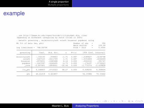
. use http://fmwww.bc.edu/repec/bocode/c/citybudget.dta, clear(Spending on different categories by Dutch cities in 2005)
. betafit governing , mu(minorityleft noleft houseval popdens) nolog
ML fit of beta (mu, phi) Number of obs = 394Wald chi2(4) = 109.99
Log likelihood = 768.06704 Prob > chi2 = 0.0000
governing Coef. Std. Err. z P>|z| [95% Conf. Interval]
minorityleft -.102143 .059603 -1.71 0.087 -.2189627 .0146768noleft .1047123 .0611709 1.71 0.087 -.0151804 .2246049
houseval .2970051 .0483488 6.14 0.000 .2022432 .391767popdens -.1247097 .0262695 -4.75 0.000 -.176197 -.0732223
_cons -2.607601 .0856001 -30.46 0.000 -2.775374 -2.439828
/ln_phi 4.168403 .0715323 58.27 0.000 4.028202 4.308604
phi 64.61219 4.621857 56.15986 74.33662
Maarten L. Buis Analyzing Proportions
A single proportionMultiple proportions
example
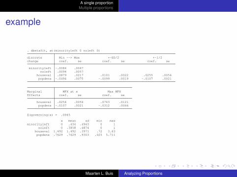
. dbetafit, at(minorityleft 0 noleft 0)
discrete Min --> Max +-SD/2 +-1/2change coef. se coef. se coef. se
minorityleft -.0084 .0047noleft .0094 .0057
houseval .0879 .0217 .0101 .0022 .0255 .0056popdens -.0494 .0075 -.0099 .0019 -.0107 .0021
Marginal MFX at x Max MFXEffects coef. se coef. se
houseval .0254 .0056 .0743 .0121popdens -.0107 .0021 -.0312 .0066
E(governing|x) = .0945
x mean sd min maxminorityleft 0 .434 .4963 0 1
noleft 0 .3858 .4874 0 1houseval 1.492 1.492 .3971 .72 3.63popdens .7629 .7629 .9303 .025 5.711
Maarten L. Buis Analyzing Proportions

A single proportionMultiple proportions
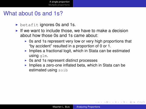
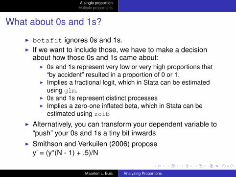
What about 0s and 1s?
I betafit ignores 0s and 1s.I If we want to include those, we have to make a decision
about how those 0s and 1s came about:I 0s and 1s represent very low or very high proportions that
“by accident” resulted in a proportion of 0 or 1.I Implies a fractional logit, which in Stata can be estimated
using glm.I 0s and 1s represent distinct processesI Implies a zero-one inflated beta, which in Stata can be
estimated using zoib
I Alternatively, you can transform your dependent variable to“push” your 0s and 1s a tiny bit inwards
I Smithson and Verkuilen (2006) proposey’ = (y*(N - 1) + .5)/N
Maarten L. Buis Analyzing Proportions

A single proportionMultiple proportions
What about 0s and 1s?
I betafit ignores 0s and 1s.
I If we want to include those, we have to make a decisionabout how those 0s and 1s came about:
I 0s and 1s represent very low or very high proportions that“by accident” resulted in a proportion of 0 or 1.
I Implies a fractional logit, which in Stata can be estimatedusing glm.
I 0s and 1s represent distinct processesI Implies a zero-one inflated beta, which in Stata can be
estimated using zoib
I Alternatively, you can transform your dependent variable to“push” your 0s and 1s a tiny bit inwards
I Smithson and Verkuilen (2006) proposey’ = (y*(N - 1) + .5)/N
Maarten L. Buis Analyzing Proportions

A single proportionMultiple proportions
What about 0s and 1s?
I betafit ignores 0s and 1s.I If we want to include those, we have to make a decision
about how those 0s and 1s came about:
I 0s and 1s represent very low or very high proportions that“by accident” resulted in a proportion of 0 or 1.
I Implies a fractional logit, which in Stata can be estimatedusing glm.
I 0s and 1s represent distinct processesI Implies a zero-one inflated beta, which in Stata can be
estimated using zoib
I Alternatively, you can transform your dependent variable to“push” your 0s and 1s a tiny bit inwards
I Smithson and Verkuilen (2006) proposey’ = (y*(N - 1) + .5)/N
Maarten L. Buis Analyzing Proportions
A single proportionMultiple proportions
What about 0s and 1s?
I betafit ignores 0s and 1s.I If we want to include those, we have to make a decision
about how those 0s and 1s came about:I 0s and 1s represent very low or very high proportions that
“by accident” resulted in a proportion of 0 or 1.
I Implies a fractional logit, which in Stata can be estimatedusing glm.
I 0s and 1s represent distinct processesI Implies a zero-one inflated beta, which in Stata can be
estimated using zoib
I Alternatively, you can transform your dependent variable to“push” your 0s and 1s a tiny bit inwards
I Smithson and Verkuilen (2006) proposey’ = (y*(N - 1) + .5)/N
Maarten L. Buis Analyzing Proportions
A single proportionMultiple proportions
What about 0s and 1s?
I betafit ignores 0s and 1s.I If we want to include those, we have to make a decision
about how those 0s and 1s came about:I 0s and 1s represent very low or very high proportions that
“by accident” resulted in a proportion of 0 or 1.I Implies a fractional logit, which in Stata can be estimated
using glm.
I 0s and 1s represent distinct processesI Implies a zero-one inflated beta, which in Stata can be
estimated using zoib
I Alternatively, you can transform your dependent variable to“push” your 0s and 1s a tiny bit inwards
I Smithson and Verkuilen (2006) proposey’ = (y*(N - 1) + .5)/N
Maarten L. Buis Analyzing Proportions
A single proportionMultiple proportions
What about 0s and 1s?
I betafit ignores 0s and 1s.I If we want to include those, we have to make a decision
about how those 0s and 1s came about:I 0s and 1s represent very low or very high proportions that
“by accident” resulted in a proportion of 0 or 1.I Implies a fractional logit, which in Stata can be estimated
using glm.I 0s and 1s represent distinct processes
I Implies a zero-one inflated beta, which in Stata can beestimated using zoib
I Alternatively, you can transform your dependent variable to“push” your 0s and 1s a tiny bit inwards
I Smithson and Verkuilen (2006) proposey’ = (y*(N - 1) + .5)/N
Maarten L. Buis Analyzing Proportions
A single proportionMultiple proportions
What about 0s and 1s?
I betafit ignores 0s and 1s.I If we want to include those, we have to make a decision
about how those 0s and 1s came about:I 0s and 1s represent very low or very high proportions that
“by accident” resulted in a proportion of 0 or 1.I Implies a fractional logit, which in Stata can be estimated
using glm.I 0s and 1s represent distinct processesI Implies a zero-one inflated beta, which in Stata can be
estimated using zoib
I Alternatively, you can transform your dependent variable to“push” your 0s and 1s a tiny bit inwards
I Smithson and Verkuilen (2006) proposey’ = (y*(N - 1) + .5)/N
Maarten L. Buis Analyzing Proportions
A single proportionMultiple proportions
Fractional logit
I 0s and 1s occur through the same process as the otherproportions
I Only models the mean, this means:I less sensitive to errors in other parts of the model, e.g. the
variance, butI not suitable when interest is in other quantities than the
mean, e.g. the varianceI Can be estimated with glm in combination with thelink(logit) family(binomial) robust options.
Maarten L. Buis Analyzing Proportions
A single proportionMultiple proportions
Fractional logit
I 0s and 1s occur through the same process as the otherproportions
I Only models the mean, this means:
I less sensitive to errors in other parts of the model, e.g. thevariance, but
I not suitable when interest is in other quantities than themean, e.g. the variance
I Can be estimated with glm in combination with thelink(logit) family(binomial) robust options.
Maarten L. Buis Analyzing Proportions
A single proportionMultiple proportions
Fractional logit
I 0s and 1s occur through the same process as the otherproportions
I Only models the mean, this means:I less sensitive to errors in other parts of the model, e.g. the
variance, but
I not suitable when interest is in other quantities than themean, e.g. the variance
I Can be estimated with glm in combination with thelink(logit) family(binomial) robust options.
Maarten L. Buis Analyzing Proportions
A single proportionMultiple proportions
Fractional logit
I 0s and 1s occur through the same process as the otherproportions
I Only models the mean, this means:I less sensitive to errors in other parts of the model, e.g. the
variance, butI not suitable when interest is in other quantities than the
mean, e.g. the variance
I Can be estimated with glm in combination with thelink(logit) family(binomial) robust options.
Maarten L. Buis Analyzing Proportions
A single proportionMultiple proportions
Fractional logit
I 0s and 1s occur through the same process as the otherproportions
I Only models the mean, this means:I less sensitive to errors in other parts of the model, e.g. the
variance, butI not suitable when interest is in other quantities than the
mean, e.g. the varianceI Can be estimated with glm in combination with thelink(logit) family(binomial) robust options.
Maarten L. Buis Analyzing Proportions
A single proportionMultiple proportions
example
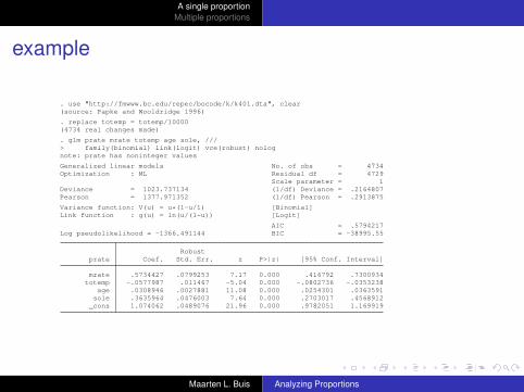
. use "http://fmwww.bc.edu/repec/bocode/k/k401.dta", clear(source: Papke and Wooldridge 1996)
. replace totemp = totemp/10000(4734 real changes made)
. glm prate mrate totemp age sole, ///> family(binomial) link(logit) vce(robust) nolognote: prate has noninteger values
Generalized linear models No. of obs = 4734Optimization : ML Residual df = 4729
Scale parameter = 1Deviance = 1023.737134 (1/df) Deviance = .2164807Pearson = 1377.971352 (1/df) Pearson = .2913875
Variance function: V(u) = u*(1-u/1) [Binomial]Link function : g(u) = ln(u/(1-u)) [Logit]
AIC = .5794217Log pseudolikelihood = -1366.491144 BIC = -38995.55
Robustprate Coef. Std. Err. z P>|z| [95% Conf. Interval]
mrate .5734427 .0799253 7.17 0.000 .416792 .7300934totemp -.0577987 .011467 -5.04 0.000 -.0802736 -.0353238
age .0308946 .0027881 11.08 0.000 .0254301 .0363591sole .3635964 .0476003 7.64 0.000 .2703017 .4568912_cons 1.074062 .0489076 21.96 0.000 .9782051 1.169919
Maarten L. Buis Analyzing Proportions
A single proportionMultiple proportions
example
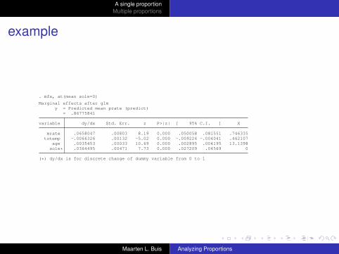
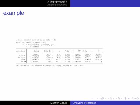
. mfx, at(mean sole=0)
Marginal effects after glmy = Predicted mean prate (predict)
= .86775841
variable dy/dx Std. Err. z P>|z| [ 95% C.I. ] X
mrate .0658047 .00803 8.19 0.000 .050058 .081551 .746335totemp -.0066326 .00132 -5.02 0.000 -.009224 -.004041 .462107
age .0035453 .00033 10.69 0.000 .002895 .004195 13.1398sole* .0364495 .00471 7.73 0.000 .027209 .04569 0
(*) dy/dx is for discrete change of dummy variable from 0 to 1
Maarten L. Buis Analyzing Proportions
A single proportionMultiple proportions
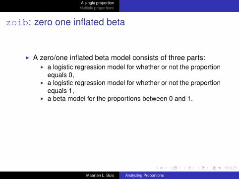
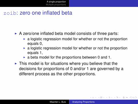
zoib: zero one inflated beta
I A zero/one inflated beta model consists of three parts:I a logistic regression model for whether or not the proportion
equals 0,I a logistic regression model for whether or not the proportion
equals 1,I a beta model for the proportions between 0 and 1.
I This model is for situations where you believe that thedecisions for proportions of 0 and/or 1 are governed by adifferent process as the other proportions.
Maarten L. Buis Analyzing Proportions
A single proportionMultiple proportions
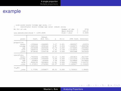
example
. zoib prate mrate totemp age sole, ///> oneinflate( mrate totemp age sole) robust nolog
ML fit of oib Number of obs = 4734Wald chi2(4) = 136.47
Log pseudolikelihood = -1293.6594 Prob > chi2 = 0.0000
Robustprate Coef. Std. Err. z P>|z| [95% Conf. Interval]
proportionmrate .1524644 .0466905 3.27 0.001 .0609527 .243976totemp -.0265332 .0092522 -2.87 0.004 -.0446673 -.0083992
age .0216248 .0020206 10.70 0.000 .0176645 .0255852sole .0604715 .0376378 1.61 0.108 -.0132972 .1342402_cons .8738362 .0354738 24.63 0.000 .8043088 .9433636
oneinflatemrate .7935556 .0653962 12.13 0.000 .6653814 .9217297totemp -.1416409 .0354509 -4.00 0.000 -.2111235 -.0721584
age .020835 .003494 5.96 0.000 .0139869 .0276832sole .9044132 .0654829 13.81 0.000 .7760692 1.032757_cons -1.472011 .0702084 -20.97 0.000 -1.609617 -1.334405
ln_phi_cons 1.77591 .0358677 49.51 0.000 1.705611 1.84621
Maarten L. Buis Analyzing Proportions
A single proportionMultiple proportions
example
. mfx, predict(pr) at(mean sole = 0)
Marginal effects after zoiby = Proportion (predict, pr)
= .85369833
variable dy/dx Std. Err. z P>|z| [ 95% C.I. ] X
mrate .0566366 .00679 8.34 0.000 .043326 .069947 .746335totemp -.0100315 .00208 -4.83 0.000 -.014104 -.005959 .462107
age .0034952 .00031 11.37 0.000 .002893 .004098 13.1398sole* .053115 .0047 11.31 0.000 .043908 .062322 0
(*) dy/dx is for discrete change of dummy variable from 0 to 1
Maarten L. Buis Analyzing Proportions
A single proportionMultiple proportions
example
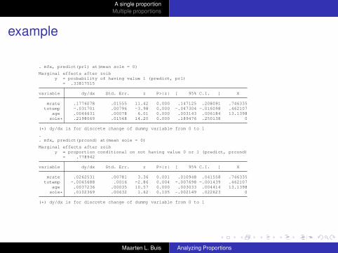
. mfx, predict(pr1) at(mean sole = 0)
Marginal effects after zoiby = probability of having value 1 (predict, pr1)
= .33817515
variable dy/dx Std. Err. z P>|z| [ 95% C.I. ] X
mrate .1776078 .01555 11.42 0.000 .147125 .208091 .746335totemp -.031701 .00796 -3.98 0.000 -.047304 -.016098 .462107
age .0046631 .00078 6.01 0.000 .003143 .006184 13.1398sole* .2198069 .01548 14.20 0.000 .189476 .250138 0
(*) dy/dx is for discrete change of dummy variable from 0 to 1
.
. mfx, predict(prcond) at(mean sole = 0)
Marginal effects after zoiby = proportion conditional on not having value 0 or 1 (predict, prcond)
= .778942
variable dy/dx Std. Err. z P>|z| [ 95% C.I. ] X
mrate .0262531 .00781 3.36 0.001 .010948 .041558 .746335totemp -.0045688 .0016 -2.86 0.004 -.007698 -.001439 .462107
age .0037236 .00035 10.57 0.000 .003033 .004414 13.1398sole* .0102369 .00632 1.62 0.105 -.002149 .022623 0
(*) dy/dx is for discrete change of dummy variable from 0 to 1
Maarten L. Buis Analyzing Proportions
A single proportionMultiple proportions
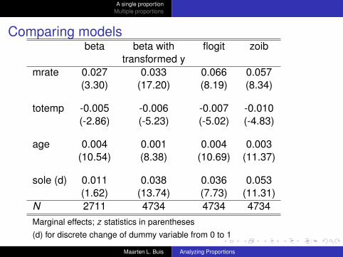
Comparing modelsbeta beta with flogit zoib
transformed ymrate 0.027 0.033 0.066 0.057
(3.30) (17.20) (8.19) (8.34)
totemp -0.005 -0.006 -0.007 -0.010(-2.86) (-5.23) (-5.02) (-4.83)
age 0.004 0.001 0.004 0.003(10.54) (8.38) (10.69) (11.37)
sole (d) 0.011 0.038 0.036 0.053(1.62) (13.74) (7.73) (11.31)
N 2711 4734 4734 4734Marginal effects; z statistics in parentheses(d) for discrete change of dummy variable from 0 to 1
Maarten L. Buis Analyzing Proportions

A single proportionMultiple proportions
Outline
A single proportion
Multiple proportions
Maarten L. Buis Analyzing Proportions
A single proportionMultiple proportions
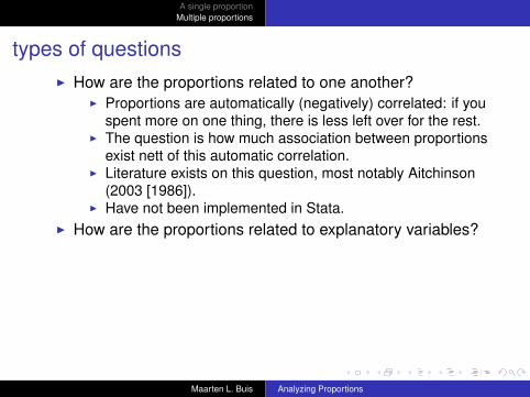
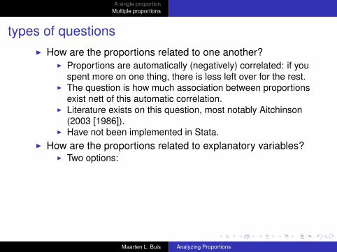
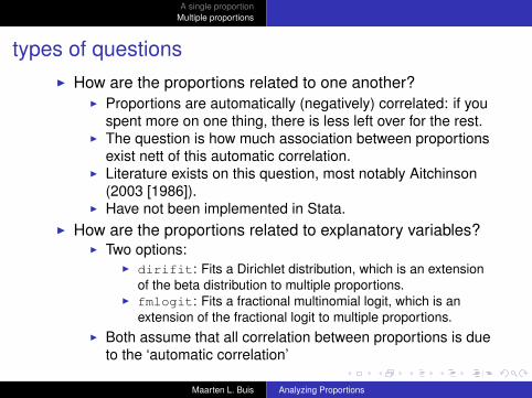
types of questionsI How are the proportions related to one another?
I Proportions are automatically (negatively) correlated: if youspent more on one thing, there is less left over for the rest.
I The question is how much association between proportionsexist nett of this automatic correlation.
I Literature exists on this question, most notably Aitchinson(2003 [1986]).
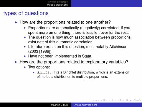
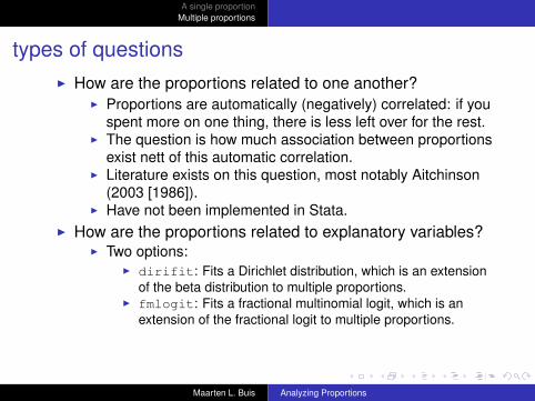
I Have not been implemented in Stata.I How are the proportions related to explanatory variables?
I Two options:I dirifit: Fits a Dirichlet distribution, which is an extension
of the beta distribution to multiple proportions.I fmlogit: Fits a fractional multinomial logit, which is an
extension of the fractional logit to multiple proportions.I Both assume that all correlation between proportions is due
to the ‘automatic correlation’
Maarten L. Buis Analyzing Proportions
A single proportionMultiple proportions
types of questionsI How are the proportions related to one another?
I Proportions are automatically (negatively) correlated: if youspent more on one thing, there is less left over for the rest.
I The question is how much association between proportionsexist nett of this automatic correlation.
I Literature exists on this question, most notably Aitchinson(2003 [1986]).
I Have not been implemented in Stata.
I How are the proportions related to explanatory variables?I Two options:
I dirifit: Fits a Dirichlet distribution, which is an extensionof the beta distribution to multiple proportions.
I fmlogit: Fits a fractional multinomial logit, which is anextension of the fractional logit to multiple proportions.
I Both assume that all correlation between proportions is dueto the ‘automatic correlation’
Maarten L. Buis Analyzing Proportions
A single proportionMultiple proportions
types of questionsI How are the proportions related to one another?
I Proportions are automatically (negatively) correlated: if youspent more on one thing, there is less left over for the rest.
I The question is how much association between proportionsexist nett of this automatic correlation.
I Literature exists on this question, most notably Aitchinson(2003 [1986]).
I Have not been implemented in Stata.I How are the proportions related to explanatory variables?
I Two options:I dirifit: Fits a Dirichlet distribution, which is an extension
of the beta distribution to multiple proportions.I fmlogit: Fits a fractional multinomial logit, which is an
extension of the fractional logit to multiple proportions.I Both assume that all correlation between proportions is due
to the ‘automatic correlation’
Maarten L. Buis Analyzing Proportions
A single proportionMultiple proportions
types of questionsI How are the proportions related to one another?
I Proportions are automatically (negatively) correlated: if youspent more on one thing, there is less left over for the rest.
I The question is how much association between proportionsexist nett of this automatic correlation.
I Literature exists on this question, most notably Aitchinson(2003 [1986]).
I Have not been implemented in Stata.I How are the proportions related to explanatory variables?
I Two options:
I dirifit: Fits a Dirichlet distribution, which is an extensionof the beta distribution to multiple proportions.
I fmlogit: Fits a fractional multinomial logit, which is anextension of the fractional logit to multiple proportions.
I Both assume that all correlation between proportions is dueto the ‘automatic correlation’
Maarten L. Buis Analyzing Proportions
A single proportionMultiple proportions
types of questionsI How are the proportions related to one another?
I Proportions are automatically (negatively) correlated: if youspent more on one thing, there is less left over for the rest.
I The question is how much association between proportionsexist nett of this automatic correlation.
I Literature exists on this question, most notably Aitchinson(2003 [1986]).
I Have not been implemented in Stata.I How are the proportions related to explanatory variables?
I Two options:I dirifit: Fits a Dirichlet distribution, which is an extension
of the beta distribution to multiple proportions.
I fmlogit: Fits a fractional multinomial logit, which is anextension of the fractional logit to multiple proportions.
I Both assume that all correlation between proportions is dueto the ‘automatic correlation’
Maarten L. Buis Analyzing Proportions
A single proportionMultiple proportions
types of questionsI How are the proportions related to one another?
I Proportions are automatically (negatively) correlated: if youspent more on one thing, there is less left over for the rest.
I The question is how much association between proportionsexist nett of this automatic correlation.
I Literature exists on this question, most notably Aitchinson(2003 [1986]).
I Have not been implemented in Stata.I How are the proportions related to explanatory variables?
I Two options:I dirifit: Fits a Dirichlet distribution, which is an extension
of the beta distribution to multiple proportions.I fmlogit: Fits a fractional multinomial logit, which is an
extension of the fractional logit to multiple proportions.
I Both assume that all correlation between proportions is dueto the ‘automatic correlation’
Maarten L. Buis Analyzing Proportions
A single proportionMultiple proportions
types of questionsI How are the proportions related to one another?
I Proportions are automatically (negatively) correlated: if youspent more on one thing, there is less left over for the rest.
I The question is how much association between proportionsexist nett of this automatic correlation.
I Literature exists on this question, most notably Aitchinson(2003 [1986]).
I Have not been implemented in Stata.I How are the proportions related to explanatory variables?
I Two options:I dirifit: Fits a Dirichlet distribution, which is an extension
of the beta distribution to multiple proportions.I fmlogit: Fits a fractional multinomial logit, which is an
extension of the fractional logit to multiple proportions.I Both assume that all correlation between proportions is due
to the ‘automatic correlation’
Maarten L. Buis Analyzing Proportions
A single proportionMultiple proportions
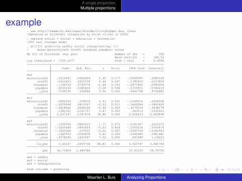
example. use http://fmwww.bc.edu/repec/bocode/c/citybudget.dta, clear(Spending on different categories by Dutch cities in 2005)
. replace social = social + education + recreation(395 real changes made)
. dirifit governing safety social urbanplanning, ///> muvar(minorityleft noleft houseval popdens) nolog
ML fit of Dirichlet (mu, phi) Number of obs = 392Wald chi2(12) = 189.54
Log likelihood = 1725.1477 Prob > chi2 = 0.0000
Coef. Std. Err. z P>|z| [95% Conf. Interval]
mu2minorityleft .1215461 .0900454 1.35 0.177 -.0549397 .2980319
noleft .0423453 .0925709 0.46 0.647 -.1390903 .2237809houseval -.104733 .0729776 -1.44 0.151 -.2477665 .0383004popdens .0030234 .0385816 0.08 0.938 -.0725951 .0786419
_cons .7199195 .129466 5.56 0.000 .4661708 .9736682
mu3minorityleft .0492506 .078676 0.63 0.531 -.1049516 .2034528
noleft -.2055446 .0813187 -2.53 0.011 -.3649264 -.0461629houseval -.4818642 .0694126 -6.94 0.000 -.6179105 -.3458179popdens .1282351 .0331747 3.87 0.000 .063214 .1932563
_cons 2.237157 .1187476 18.84 0.000 2.004415 2.469898
mu4minorityleft .1530504 .0863215 1.77 0.076 -.0161367 .3222375
noleft -.0205669 .0891623 -0.23 0.818 -.1953218 .1541879houseval -.1563326 .070531 -2.22 0.027 -.2945709 -.0180943popdens .1285933 .0354878 3.62 0.000 .0590385 .1981481
_cons .9378096 .1247067 7.52 0.000 .693389 1.18223
/ln_phi 3.60327 .0405736 88.81 0.000 3.523747 3.682792
phi 36.71809 1.489786 33.91125 39.75726
mu2 = safetymu3 = socialmu4 = urbanplanning
base outcome = governing
Maarten L. Buis Analyzing Proportions

A single proportionMultiple proportions
example
. ddirifit, at(minorityleft 0 noleft 0 )
discrete Min --> Max +-SD/2 +-1/2change coef. se coef. se coef. se
governingminorityleft -.0078 .0066
noleft .0099 .0074houseval .0937 .0233 .0115 .0024 .0293 .0062popdens -.0461 .0115 -.0087 .0027 -.0093 .0029
safetyminorityleft .0072 .0088
noleft .0257 .0096houseval .0926 .0254 .013 .003 .0333 .0077popdens -.0792 .0152 -.0149 .0035 -.0159 .0037
socialminorityleft -.0159 .0114
noleft -.0527 .012houseval -.264 .0304 -.0366 .0045 -.0935 .0114popdens .0865 .0251 .0164 .0042 .0174 .0045
urbanplann~gminorityleft .0165 .0097
noleft .0171 .0102houseval .0777 .0265 .0121 .0033 .0309 .0085popdens .0387 .0219 .0073 .0034 .0078 .0036
Maarten L. Buis Analyzing Proportions

A single proportionMultiple proportions
example
Marginal MFX at xEffects coef. se
governinghouseval .0293 .0061popdens -.0093 .0029
safetyhouseval .0334 .0077popdens -.0159 .0037
socialhouseval -.0937 .0115popdens .0174 .0045
urbanplann~ghouseval .031 .0085popdens .0078 .0035
E(governing|x) = .0993E(safety|x) = .175E(social|x) = .5032E(urbanplann~g|x) = .2225
x mean sd min maxminorityleft 0 .4337 .4962 0 1
noleft 0 .3878 .4879 0 1houseval 1.483 1.483 .3902 .72 3.63popdens .7839 .7839 .9408 .025 5.711
Maarten L. Buis Analyzing Proportions
A single proportionMultiple proportions
example
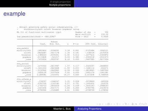
. fmlogit governing safety social urbanplanning, ///> eta(minorityleft noleft houseval popdens) nolog
ML fit of fractional multinomial logit Number of obs = 392Wald chi2(12) = 232.02
Log pseudolikelihood = -480.22927 Prob > chi2 = 0.0000
RobustCoef. Std. Err. z P>|z| [95% Conf. Interval]
eta_safetyminorityleft .1893804 .0596091 3.18 0.001 .0725486 .3062121
noleft .0826287 .0617178 1.34 0.181 -.038336 .2035934houseval -.1389243 .0555301 -2.50 0.012 -.2477614 -.0300872popdens .0115828 .021217 0.55 0.585 -.0300018 .0531673
_cons .7472656 .0920767 8.12 0.000 .5667985 .9277326
eta_socialminorityleft .1274304 .0813587 1.57 0.117 -.0320297 .2868905
noleft -.1631202 .0843848 -1.93 0.053 -.3285114 .002271houseval -.5152946 .0849965 -6.06 0.000 -.6818845 -.3487046popdens .1456129 .0257634 5.65 0.000 .0951176 .1961081
_cons 2.289081 .1415551 16.17 0.000 2.011638 2.566524
eta_urbanp~gminorityleft .234597 .1064367 2.20 0.028 .0259849 .443209
noleft .0302709 .1142185 0.27 0.791 -.1935932 .254135houseval -.1766753 .0856439 -2.06 0.039 -.3445343 -.0088163popdens .1601436 .0417171 3.84 0.000 .0783796 .2419076
_cons .9790566 .1526485 6.41 0.000 .6798709 1.278242
Maarten L. Buis Analyzing Proportions
A single proportionMultiple proportions
example
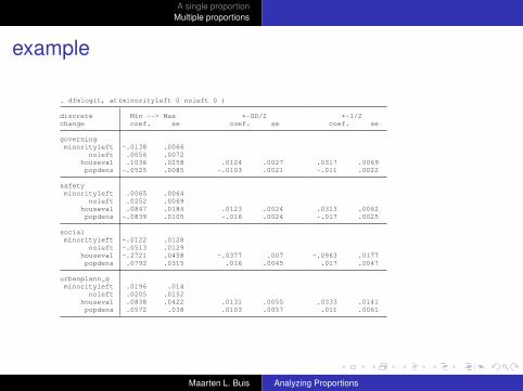
. dfmlogit, at(minorityleft 0 noleft 0 )
discrete Min --> Max +-SD/2 +-1/2change coef. se coef. se coef. se
governingminorityleft -.0138 .0066
noleft .0056 .0072houseval .1036 .0258 .0124 .0027 .0317 .0069popdens -.0525 .0085 -.0103 .0021 -.011 .0022
safetyminorityleft .0065 .0064
noleft .0252 .0069houseval .0847 .0184 .0123 .0024 .0313 .0062popdens -.0839 .0105 -.016 .0024 -.017 .0025
socialminorityleft -.0122 .0128
noleft -.0513 .0129houseval -.2721 .0458 -.0377 .007 -.0963 .0177popdens .0792 .0315 .016 .0045 .017 .0047
urbanplann~gminorityleft .0196 .014
noleft .0205 .0152houseval .0838 .0422 .0131 .0055 .0333 .0141popdens .0572 .038 .0103 .0057 .011 .0061
Maarten L. Buis Analyzing Proportions
A single proportionMultiple proportions
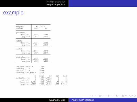
example
Marginal MFX at xEffects coef. se
governinghouseval .0317 .0065popdens -.011 .0024
safetyhouseval .0314 .0061popdens -.017 .0026
socialhouseval -.0966 .0178popdens .017 .0047
urbanplann~ghouseval .0335 .0139popdens .011 .006
E(governing|x) = .098E(safety|x) = .1699E(social|x) = .5046E(urbanplann~g|x) = .2276
x mean sd min maxminorityleft 0 .4337 .4962 0 1
noleft 0 .3878 .4879 0 1houseval 1.483 1.483 .3902 .72 3.63popdens .7839 .7839 .9408 .025 5.711
Maarten L. Buis Analyzing Proportions
Summary
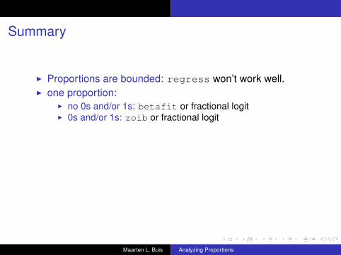
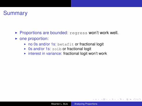
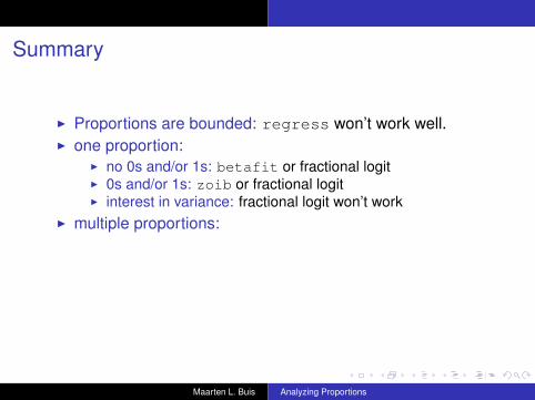
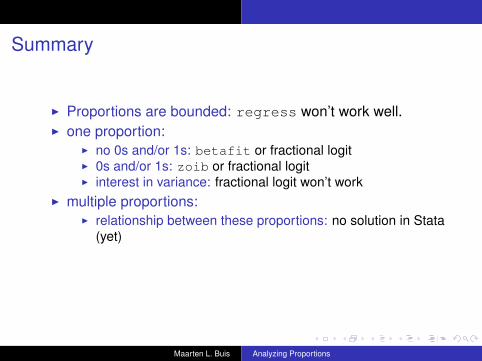
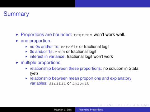
I Proportions are bounded: regress won’t work well.
I one proportion:I no 0s and/or 1s: betafit or fractional logitI 0s and/or 1s: zoib or fractional logitI interest in variance: fractional logit won’t work
I multiple proportions:I relationship between these proportions: no solution in Stata
(yet)I relationship between mean proportions and explanatory
variables: dirifit or fmlogit
Maarten L. Buis Analyzing Proportions
Summary
I Proportions are bounded: regress won’t work well.I one proportion:
I no 0s and/or 1s: betafit or fractional logitI 0s and/or 1s: zoib or fractional logitI interest in variance: fractional logit won’t work
I multiple proportions:I relationship between these proportions: no solution in Stata
(yet)I relationship between mean proportions and explanatory
variables: dirifit or fmlogit
Maarten L. Buis Analyzing Proportions
Summary
I Proportions are bounded: regress won’t work well.I one proportion:
I no 0s and/or 1s: betafit or fractional logit
I 0s and/or 1s: zoib or fractional logitI interest in variance: fractional logit won’t work
I multiple proportions:I relationship between these proportions: no solution in Stata
(yet)I relationship between mean proportions and explanatory
variables: dirifit or fmlogit
Maarten L. Buis Analyzing Proportions
Summary
I Proportions are bounded: regress won’t work well.I one proportion:
I no 0s and/or 1s: betafit or fractional logitI 0s and/or 1s: zoib or fractional logit
I interest in variance: fractional logit won’t workI multiple proportions:
I relationship between these proportions: no solution in Stata(yet)
I relationship between mean proportions and explanatoryvariables: dirifit or fmlogit
Maarten L. Buis Analyzing Proportions
Summary
I Proportions are bounded: regress won’t work well.I one proportion:
I no 0s and/or 1s: betafit or fractional logitI 0s and/or 1s: zoib or fractional logitI interest in variance: fractional logit won’t work
I multiple proportions:I relationship between these proportions: no solution in Stata
(yet)I relationship between mean proportions and explanatory
variables: dirifit or fmlogit
Maarten L. Buis Analyzing Proportions
Summary
I Proportions are bounded: regress won’t work well.I one proportion:
I no 0s and/or 1s: betafit or fractional logitI 0s and/or 1s: zoib or fractional logitI interest in variance: fractional logit won’t work
I multiple proportions:
I relationship between these proportions: no solution in Stata(yet)
I relationship between mean proportions and explanatoryvariables: dirifit or fmlogit
Maarten L. Buis Analyzing Proportions
Summary
I Proportions are bounded: regress won’t work well.I one proportion:
I no 0s and/or 1s: betafit or fractional logitI 0s and/or 1s: zoib or fractional logitI interest in variance: fractional logit won’t work
I multiple proportions:I relationship between these proportions: no solution in Stata
(yet)
I relationship between mean proportions and explanatoryvariables: dirifit or fmlogit
Maarten L. Buis Analyzing Proportions
Summary
I Proportions are bounded: regress won’t work well.I one proportion:
I no 0s and/or 1s: betafit or fractional logitI 0s and/or 1s: zoib or fractional logitI interest in variance: fractional logit won’t work
I multiple proportions:I relationship between these proportions: no solution in Stata
(yet)I relationship between mean proportions and explanatory
variables: dirifit or fmlogit
Maarten L. Buis Analyzing Proportions
References
Aitchison, J.The Statistical Analysis of Compositional Data.Caldwell, NJ: The Blackburn Press, 2003 [1986].
Ferrari, S.L.P. and Cribari-Neto, F.Beta regression for modelling rates and proportions.Journal of Applied Statistics, 31(7): 799–815, 2004.
Paolino, P.Maximum likelihood estimation of models with beta-distributed dependent variables.Political Analysis, 9(4): 325–346, 2001.
Papke, L.E. and Wooldridge, J.M.Econometric Methods for Fractional Response Variables with an Application to 401(k) Plan ParticipationRates.Journal of Applied Econometrics, 11(6):619–632, 1996.
Smithson, M. and Verkuilen, J.A better lemon squeezer? Maximum likelihood regression with beta-distributed dependent variables.Psychological Methods, 11(1):54–71, 2006.
Maarten L. Buis Analyzing Proportions