Inspecting the Mechanism:

Leverage and the Great Recession in the Eurozone∗

Philippe Martin and Thomas Philippon†

February 2015

Abstract

We provide a first comprehensive account of the dynamics of Eurozone countries from the creation of the

Euro to the Great recession. We model each country as an open economy within a monetary union and

analyze the dynamics of private leverage, fiscal policy and spreads. A parsimonious model can replicate

the time-series of nominal GDP, employment, and net exports of Eurozone countries between 2000 and

2012. We then ask how periphery countries would have fared with: (i) more conservative fiscal policies;

(ii) macro-prudential tools to control private leverage; (iii) a central bank acting earlier to limit financial

segmentation; and (iv) effective fiscal devaluation. To perform these counterfactual experiments, we use

U.S. states as a control group that did not suffer from a sudden stop. We find that periphery countries

could have stabilized their employment if they had followed more conservative fiscal policies during the

boom. This is especially true in Greece. For Ireland, however, given the size of the private leverage

boom, such a policy would have required buying back almost all of the public debt. Macro-prudential

policy would have been especially helpful in Ireland and Spain. However, in presence of a spending bias

in fiscal rules, macro-prudential policies would have led to less prudent fiscal policies in the boom. If

spreads had not spiked, employment would have been stabilized in all countries because they would not

have been constrained into fiscal austerity. Finally, a fall in export prices - through a fiscal devaluation

- would have enabled countries to attenuate the employment bust and to reduce their public debt.

∗We thank Nobu Kiyotaki, Fiorella De Fiore, Emi Nakamura, Vania Stavrakeva, Ivan Werning and Philip Lane for theirdiscussions, as well as Mark Aguiar, Olivier Blanchard, Giovanni Dell’Arricia, Gita Gopinath, Gianluca Violante, CaterinaMendicino, Mark Gertler, Virgiliu Midrigan and seminar participants at AEA, NY Fed, NYU, Harvard, Berkeley, Banquede France, CREI, ECB, Warwick, ESSIM-CEPR and the NBER for their comments. Joseba Martinez provided outstandingresearch assistance. We thank the Fondation Banque de France for financial support. Philippe Martin is also grateful to theBanque de France Sciences Po partnership for its financial support.†Sciences Po and CEPR, New York University, CEPR and NBER

1

The lesson to be learned from the crisis is that a currency union needs ironclad budget discipline

to avert a boom-and-bust cycle in the first place. Hans Werner Sinn (2010)

On the eve of the crisis (Spain) had low debt and a budget surplus. Unfortunately, it also had an

enormous housing bubble, a bubble made possible in large part by huge loans from German banks

to their Spanish counterparts. Paul Krugman (2012)

The situation of Spain is reminiscent of the situation of emerging economies that have to borrow

in a foreign currency...they can suddenly be confronted with a “sudden stop” when capital inflows

suddenly stop leading to a liquidity crisis. Paul de Grauwe (2012)

Countries which lost competitiveness prior to the crisis experienced the lowest growth after the

crisis. Lorenzo Bini Smaghi (2013)

These quotes illustrate the wide disagreement about the nature of the eurozone crisis. Some see the crisis as

driven by fiscal indiscipline, some emphasize excessive private leverage, while others focus on sudden stops

or competitiveness divergence due to fixed exchange rates. Most observers understand that all these “usual

suspects” have played a role, but do not offer a way to quantify their respective importance. In this context it

is difficult to frame policy prescriptions on macroeconomic policies and on reforms of the eurozone. Moreover,

given the scale of the crisis, understanding the dynamics of the Eurozone is one of the major challenge for

macroeconomics today. This requires a quantitative framework to identify the various mechanisms at play.

The ultimate goal of this paper is to perform counterfactual experiments. For instance, we want to

understand what would have happened to a particular country if it had run a different fiscal policy during

the boom years, or if the eurozone had figured out a way to prevent sudden stops. Our contribution is to

propose a model and an identification strategy to answer these questions. Needless to say, this is a difficult

task that requires several steps: (i) specify a model and collect the data; (ii) find an identification strategy;

(iii) run counterfactual experiments. This is what we do.

One feature of our analysis needs to be explained immediately to avoid confusion: we do not attempt

to explain the average dynamics of the currency union. Instead, we study the relative dynamics of each

country within the eurozone. Our model explains the impact of a sudden stop, say, on employment in Spain

versus employment in Germany. In our control group, we focus on the dynamics of each state within the

United States. This is how we identify our model and how we can make progress, but it is also obviously a

limitation of our analysis. We do not claim to have a fully structural analysis of the eurozone crisis, but we

claim that all the steps we take in this paper are necessary for such a structural analysis.

2

Our model focuses on three variables: private debt, fiscal policy, and funding costs. We analyze a

collection of small open economies in a monetary union. Each economy has an independent fiscal policy

and is populated by patient and impatient agents. Impatient agents borrow from patient agents but are

subject to a time-varying borrowing limit. Governments tax, spend, and borrow. Funding costs are linked

to private and public debt sustainability. Nominal wage are rigid so that changes in nominal expenditures

affect employment. Our first contribution is to show that this parsimonious model does a fairly good job

at replicating the dynamics of each individual eurozone country over the 13 years for which we have data.

More precisely, given the paths of private debt, government spending and interest rates from 2000 to 2012,

the model predicts the correct paths for GDP, employment, inflation, net exports, etc.

It is clear, however, that private debt, fiscal policy and funding costs are jointly endogenous. A key

challenge is then to identify structural shocks that give rise to the observed dynamics. For instance, we would

like to identify “sudden stop” shocks, and “private lending” shocks. But both shocks are going to affect interest

rates, private debt, and they will also affect fiscal policy and public debt via general equilibrium effects and

policy responses. Our key idea is to use the United States as a control group to help us identify shocks within

the eurozone. The U.S. experience is of great interest for us because of both its similarities and its differences

with the eurozone experience. A salient feature of the great recession in both the US and the eurozone is that

regions that have experienced the largest swings in household borrowing have also experienced the largest

declines in employment and output. Figure 1 illustrates this feature of the data, by plotting the change

in employment during the credit crunch (2007-2010) against the change in household debt-to-income ratios

during the preceding boom (2003-2007) for the largest US states and Eurozone countries.1

Until 2010, the American and European experiences look strikingly similar. This suggests both similar

shocks and similar structural parameters governing the endogenous propagation mechanism. A significant

difference between the two regions appears only after 2010 when several eurozone countries experience sudden

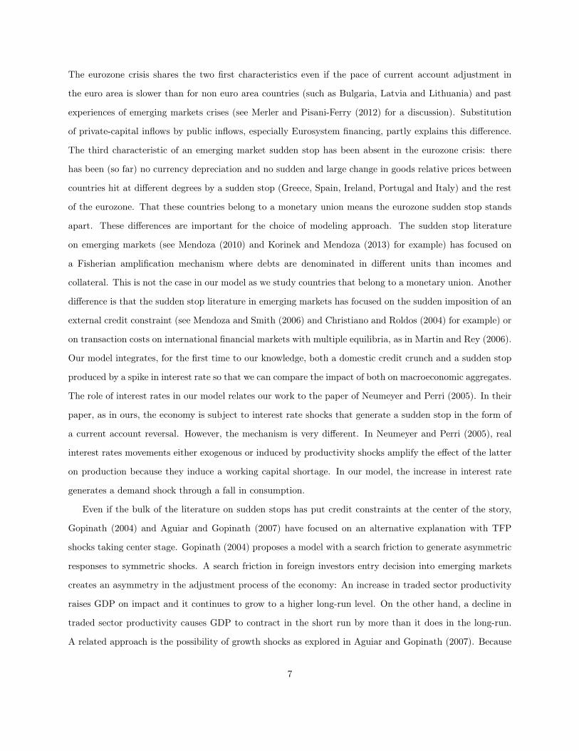
stops and sovereign debt crises.2 Consider for example Arizona and Ireland. Both had large increases in

household debt during the boom years. Figure 2 shows the evolutions of their employment rates relative to

2005. The boom-bust cycle is almost identical up to 2010 but diverges afterwards. A similar pattern emerges

when we compare Spain and Florida. Again, divergence is clear after 2010.1State level household debt for the US comes from the Federal Reserve Bank of New York, see Midrigan and Philippon

(2010). Nominal (wage) rigidities play an important role in our model. As noted in Midrigan and Philippon (2010), the patternof figure 1 is at odds with the predictions of standard models of financing frictions with flexible wages. Such models predictthat a tightening of borrowing constraints at the household level leads to a decline in consumption but, due to wealth effects,to an increase in the supply of labor.

2Sudden stops have been frequent in the 19th and 20th centuries but we do not know of any other historical example of asudden stop among countries or states inside a monetary union. See Accominotti and Eichengreen (2013).

3

Figure 1: First Stage of the Great Recession: Household Borrowing predicts Employment Bust in the USand the EZ

AZ

CA

FL

IL

MI

NJ

NV

NY

OH

PATX

USA

AUT

BEL

DEU

ESP

FIN

FRA GRE

IRL

ITA

NLD

PRT

−.0

6−

.04

−.0

20

.02

Change E

mp/P

op 2

007−

2009

−.1 .1 .3 .5Change Household Debt/GDP 2003−2007

Many states within the U.S. experienced large private leveraging/deleveraging cycle. This allows us to

identify debt dynamics that are not due to interest rate spreads, i.e., the private debt dynamics that would

have prevailed across the eurozone if it had not experienced a sudden stop. This is our most important

and novel identification strategy. Our other identifying assumptions are more standard. We assume a fiscal

rule that stabilizes employment and reacts to funding costs, and we introduce a country-specific spending

bias, which we called the “political economy” factor. Together with the fiscal rule, it predicts government

spending as a function of the state of the economy. We estimate a small (essentially zero) political economy

bias in some countries, such as Germany and Portugal, and a large one in some other countries, such as

Greece for instance. Finally, we think of “sudden stops” as a latent risk that grows after 2008 and we show

that it materializes in countries with high public and private debts, including implicit liabilities via bank

recapitalization needs. We use instrumental variables to estimate the impact of public and private debts on

the economy’s cost of fund.

Our “structural” model therefore features endogenous private debt, endogenous fiscal policy and endoge-

nous spreads. We show that this structural model fits the data fairly well. The critical advantage of the

structural model – compared to the model that takes as given the paths of private debt, government spending

and interest rates, as explained above – is that we can use the structural model to perform counterfactual

4

Figure 2: Employment Rates in Ireland, Arizona, Spain and Florida.−

.08

−.0

6−

.04

−.0

20

.02

2000 2004 2008 2012year

Ireland Arizona

Employment

−.0

6−

.04

−.0

20

.02

2000 2004 2008 2012year

Spain Florida

Employment

experiments. We perform four such experiments.

We first ask how countries would have fared if they had followed more conservative fiscal policies during

the boom. To do so, we shut down the “political economy spending bias” of the structural model. We find

that such policies lowered spreads and the need for fiscal austerity during the bust. We find that periphery

countries would then have stabilized their employment. This is especially true for Greece, and to a lesser

extent for Ireland and Spain. For Ireland, however, this more conservative policy would have entailed buying

back the entire stock of public debt, which seems implausible. This suggests that fiscal policy alone cannot

act as a stabilization tool in presence of a massive private credit boom. Most of these results are consistent

with many policy makers’ beliefs about the crisis, but we are the first to formalize and quantify them.

We then ask how these countries would have fared if they had conducted macro-prudential policies to

limit private leverage during the boom. This would have successfully stabilized employment, in part because

this would have decreased the need for bank recapitalization, leading to lower spreads and more room

for countercyclical fiscal policy. We also highlight a new interaction between macro-prudential and fiscal

policies. For a given political economy bias, a government would substitute public debt to private debt in

response to restrictive macro-prudential policy. This suggests a complementarity between fiscal rules and

macro-prudential rules.

In a third counterfactual, we find that if the ECB words and actions (Mario Draghi’s declaration “What-

ever it takes” and the OMT program) had come in 2008 rather than 2012 and had been successful in

reducing the spreads, the four countries would have been able to avoid the latest part of the employment

slump. Ireland’s employment, for instance, would have looked very much like Arizona’s in Figure (2). The

5

improvement comes from lower funding costs for the private sector and from less fiscal austerity. In Greece,

however, an unconditional OMT would have led to a return of high and unsustainable government spending.

This highlights the need for conditionality when central banks intervene.

In our last counterfactual, we let countries engineer a 10% fiscal devaluation in 2009 that generates a

boom in exports. We find that they would have experienced a shorter and milder bust and a smaller buildup

in public debt.

Relation to the literature

Our paper is related to three lines of research: (i) macroeconomic models with credit frictions, (ii)

monetary economics, (iii) sudden stops and sovereign defaults. We discuss the connections of our paper to

each topic. Following Bernanke and Gertler (1989), many macroeconomic papers introduce credit constraints

at the entrepreneur level (Kiyotaki and Moore (1997), Bernanke et al. (1999), or Cooley et al. (2004)). In all

these models, the availability of credit limits corporate investment. As a result, credit constraints affect the

economy by affecting the size of the capital stock. Curdia and Woodford (2009) analyze the implication for

monetary policy of imperfect intermediation between borrowers and lenders. Gertler and Kiyotaki (2010)

study a model where shocks that hit the financial intermediation sector lead to tighter borrowing constraints

for entrepreneurs. We model shocks in a similar way. The difference is that our borrowers are households,

not entrepreneurs, and, we argue, this makes a difference for the model’s cross-sectional implications. Models

that emphasize firm-level frictions cannot reproduce the strong correlation between household-leverage and

employment at the micro-level, unless the banking sector is island-specific, as in the small open economy

“Sudden Stop” literature (Chari et al. (2005), Mendoza (2010)). This “local lending channel” does not appear

to be operative across U.S. states, however, presumably because business lending is not very localized3. Our

framework is also related to heterogeneous-agent macroeconomic models such as Krusell and Smith (1998),

and models in the tradition of Campbell and Mankiw (1989), that feature impatient and patient consumers.

This type of models has been used by Gali et al. (2007) to analyze the impact of fiscal policy on consumption

and by Eggertsson and Krugman (2012) to analyze macroeconomic dynamics during the Great Recession.

Papers in the sudden stop literature have aimed at reproducing the stylized facts of these crises in emerging

markets. According to Korinek and Mendoza (2013) the key characteristics of a sudden stop are 1) a sharp,

sudden reversal in international capital flows, which is typically measured as a sudden increase in the current

account 2) a deep recessions and 3) sharp changes in relative prices, including exchange rate depreciations.3For instance, Mian and Sufi (2010) find that the predictive power of household borrowing remains the same in counties

dominated by national banks. It is also well known that businesses entered the recession with historically strong balanced sheetsand were able to draw on existing credit lines Ivashina and Scharfstein (2008).

6

The eurozone crisis shares the two first characteristics even if the pace of current account adjustment in

the euro area is slower than for non euro area countries (such as Bulgaria, Latvia and Lithuania) and past

experiences of emerging markets crises (see Merler and Pisani-Ferry (2012) for a discussion). Substitution

of private-capital inflows by public inflows, especially Eurosystem financing, partly explains this difference.

The third characteristic of an emerging market sudden stop has been absent in the eurozone crisis: there

has been (so far) no currency depreciation and no sudden and large change in goods relative prices between

countries hit at different degrees by a sudden stop (Greece, Spain, Ireland, Portugal and Italy) and the rest

of the eurozone. That these countries belong to a monetary union means the eurozone sudden stop stands

apart. These differences are important for the choice of modeling approach. The sudden stop literature

on emerging markets (see Mendoza (2010) and Korinek and Mendoza (2013) for example) has focused on

a Fisherian amplification mechanism where debts are denominated in different units than incomes and

collateral. This is not the case in our model as we study countries that belong to a monetary union. Another

difference is that the sudden stop literature in emerging markets has focused on the sudden imposition of an

external credit constraint (see Mendoza and Smith (2006) and Christiano and Roldos (2004) for example) or

on transaction costs on international financial markets with multiple equilibria, as in Martin and Rey (2006).

Our model integrates, for the first time to our knowledge, both a domestic credit crunch and a sudden stop

produced by a spike in interest rate so that we can compare the impact of both on macroeconomic aggregates.

The role of interest rates in our model relates our work to the paper of Neumeyer and Perri (2005). In their

paper, as in ours, the economy is subject to interest rate shocks that generate a sudden stop in the form of

a current account reversal. However, the mechanism is very different. In Neumeyer and Perri (2005), real

interest rates movements either exogenous or induced by productivity shocks amplify the effect of the latter

on production because they induce a working capital shortage. In our model, the increase in interest rate

generates a demand shock through a fall in consumption.

Even if the bulk of the literature on sudden stops has put credit constraints at the center of the story,

Gopinath (2004) and Aguiar and Gopinath (2007) have focused on an alternative explanation with TFP

shocks taking center stage. Gopinath (2004) proposes a model with a search friction to generate asymmetric

responses to symmetric shocks. A search friction in foreign investors entry decision into emerging markets

creates an asymmetry in the adjustment process of the economy: An increase in traded sector productivity

raises GDP on impact and it continues to grow to a higher long-run level. On the other hand, a decline in

traded sector productivity causes GDP to contract in the short run by more than it does in the long-run.

A related approach is the possibility of growth shocks as explored in Aguiar and Gopinath (2007). Because

7

of the income effect, a negative shock leads to a fall in consumption and an increase in the trade balance.

Aguiar and Gopinath (2007) do not study the response of the labor market but it is well known that income

effects tend move consumption and hours in opposite directions.

Shocks to trend TFP growth might be important in emerging markets, but they do not seem to explain

the dynamics of euro area countries over the past five years. With the exception of Greece, countries that

were hit by a sudden stop (Greece, Ireland, Italy, Spain, Portugal) are not those for which the reversal in

TFP growth is the largest between the boom and the bust periods and no correlation appears between the

differential in TFP growth (between the periods 2008-2012 and 2000-2007) and employment growth during

the bust (2008-2012) as illustrated by figure 30 in Appendix B.

Most closely connected to our paper is the work of Midrigan and Philippon (2010), Guerrieri and Loren-

zoni (2010) and Eggertsson and Krugman (2012) who also study the responses of an economy to a household-

level credit crunch. Consistent with our results, Mian and Sufi (2012) show that differences in the debt

overhang of households across U.S. counties partly explain why unemployment is higher in some regions

than others. Schmitt-Grohe and Uribe (2012) emphasize the role of downward wage rigidity in the Eurozone

recession. Our paper is also related to the literature on sovereign default (see Eaton and Gersovitz (1982),

Arellano (2008) and Mendoza and Yue (2012)) that models default as a strategic decision with a tradeoff

between gains from forgone repayment and the costs of exclusion from international credit markets. The ob-

jective of our paper however is to analyze how the sovereign default risk can affect the real economy through

the impact it can have on liquidity available to households. The paper by Corsetti et al. (2013) considers a

“sovereign risk channel,” through which sovereign default risk spills over to the rest of the economy, raising

funding costs in the private sector. Finally the paper is related to the recent research on fiscal multipliers at

the regional level (Nakamura and Steinsson (2014), Farhi and Werning (2013)).

In Section 1 we present the model and in section 2 we analyze its dynamic properties. 3 presents the

calibration exercise and compares the reduced form model predictions to the data. In Section 4, we present

the structural relations between private leverage, fiscal policy and sudden stops. These serve to conduct the

final exercise on counterfactual policies presented in section 5. Section 6 concludes.

1 Model

We model a currency union with several regions. We follow Gali and Monacelli (2008) and study a small

open economy that trades with other regions. Each region j produces a tradable domestic good and is

8

populated by households who consume the domestic good and a basket of foreign goods. Following Mankiw

(2000) and more recently Eggertsson and Krugman (2012), we assume that households are heterogenous in

their degree of time preference. More precisely, in region j, there is a fraction χj of impatient households,

and 1 − χj of patient ones. Patient households (indexed by i = s for savers) have a higher discount factor

than borrowers (indexed by i = b for borrowers): β ≡ βs > βb. Saving and borrowing are measured in units

of the common currency (euros).

1.1 Within period trade and production.

Consider household i in region j at time t. Within period, all households have the same log preferences over

the consumption of home (h), foreign goods (f), and labor supply:

ui,j,t = αj log

(Chi,j,tαj

)+ (1− αj) log

(Cfi,j,t

1− αj

)− ν (Ni,j,t)

With these preferences, households of region j spend a fraction αj of their income on home goods, and

1 − αj on foreign goods. The parameter αj measures how closed the economy is, because of home bias in

preferences or trade costs. The demand functions are then:

phj,tChi,j,t = αjXi,j,t,

pft Cfi,j,t = (1− αj)Xi,j,t.

where

Xi,j,t ≡ phj,tChi,j,t + pft Cfi,j,t

measures the spending of household i in region j in period t, phj,t is the price of home goods in country j and

pft is the price index of foreign goods. This gives the indirect utility

U (Xi,j,t, Pj,t) = log (Xi,j,t)− logPj,t − ν (Ni,j,t) ,

where the CPI of country j is logPj,t = αj log phj,t + (1− αj) log pfj,t, the PPI is phj,t, and the terms of trade

are pftphj,t

. Foreign demand for the home good also has a unit elasticity with respect to export price phj,t.

Production is linear in labor Nj,t and competitive, so phj,t = wj,t. Market clearing in the goods market

9

requires

Nj,t = χjChb,j,t + (1− χj)Chs,j,t +

Fj,tphj,t

+Gj,tphj,t

,

where Fj,t is foreign demand and Gj,t are nominal government expenditures. Note that we assume that the

government spends only on domestic goods. Define nominal domestic product as

Yj,t ≡ phj,tNj,t

and total private expenditures as

Xj,t ≡ χjXb,j,t + (1− χj)Xs,j,t.

It is useful to write the market clearing condition in nominal terms (in euros)

Yjt = αjXj,t + Fj,t +Gj,t. (1)

Each household supplies labor at the prevailing wage and receives wage income net of taxes (1− τj,t)wj,tNj,t.

They also receive transfers from the government Zj,t. We assume that wages are sticky and we ration the

labor market uniformly across households. This assumption simplifies the analysis because we do not need

to keep track separately of the labor income of patient and impatient households within a country. Not much

changes if we relax this assumption, except that we loose some tractability.4

1.2 Inter-temporal budget constraints

Let Bj,t be the face value of the debt issued in period t− 1 by impatient households and due in period t. It

will be convenient to define disposable income (after tax and transfers but before interest payments) as

Yj,t ≡ (1− τj,t)Yj,t + Zj,t.

The budget constraint of impatient households in countryj is then4In response to a negative shock, impatient households would try to work more. The prediction that hours increase more

for credit constrained households appears to be counter-factual however. One can fix this by assuming a low elasticity of laborsupply, which essentially boils down to assuming that hours worked are rationed uniformly in response to slack in the labormarket. Assuming that the elasticity of labor supply is small (near zero) also means that the natural rate does not depend onfiscal policy. In an extension we study the case where the natural rate is defined by the labor supply condition in the pseudo-steady state ν′

(n?i

)= (1− τj)

wj

xi,j. We can then ration the labor market relative to their natural rate: ni,j,t =

n?i (τ)∑

i n?i (τ)

nj,t

where n?i (τ) is the natural rate for household i in country. This ensures consistency and convergence to the correct long runequilibrium. Steady state changes in the natural rate are quantitatively small, however, so the dynamics that we study arevirtually unchanged. See Midrigan and Philippon (2010) for a discussion.

10

Bj,t+1

1 + rj,t+ Yj,t = Xb,j,t +Bj,t, (2)

where rj,t is the nominal cost of fund between t and t + 1. Notice that the budget constraint is written

without the possibility of default by the borrower. In such a case, and without taking into account issues of

market liquidity, the cost of fund is the same as the interest rate. When we discuss the model, we therefore

refer to rj,t as the interest rate. But when we turn to the data, it is obviously critical to remember that rj,t

is really meant to capture the cost of funds. We assume that interest rates are time-varying and potentially

country-specific. Borrowing is subject to the exogenous limit Bhj,t:

Bj,t ≤ Bhj,t. (3)

The savers budget constraint is:

Sj,t + Yj,t = Xs,j,t +Sj,t+1

1 + rj,t, (4)

so their Euler equation is1

Xs,j,t= Et

[β (1 + rj,t)

Xs,j,t+1

]. (5)

Note that financial markets clear in two ways in our model. For the impatient agents, given that they are

quantity constrained, interest rates do not affect their borrowing. For the patient agents, their saving is

determined by the interest rates through the Euler equation.

The government budget constraint is:

Bgj,t+1

1 + rj,t+ τj,tYjt = Gj,t + Zj,t +Bgj,t, (6)

where Bgj,t is public debt issued by government j at time t− 1.

1.3 Exports and foreign assets

Nominal exports are Fj,t and nominal imports are (1− αj)Xj,t since the government does not buy imported

goods while private agents spend a fraction 1− αj on foreign goods. So net exports are:

Ej,t = Fj,t − (1− αj)Xj,t. (7)

11

The net foreign asset position of the country at the end of period t, measured in market value, is:

Aj,t ≡ (1− χj)Sj,t+1

1 + rj,t− χj

Bhj,t+1

1 + rj,t−

Bgj,t+1

1 + rj,t. (8)

Adding up the budget constraints, we have the spending equation

Xj,t +Gj,t = Yj,t + χj

(Bhj,t+1

1 + rj,t−Bhj,t

)− (1− χj)

(Sj,t+1

1 + rj,t− Sj,t

)+

Bgj,t+1

1 + rj,t−Bgj,t (9)

Total spending (public and private) equals total income (nominal GDP) plus total net borrowing. If we

combine with the market clearing condition (1), we get the current account condition

CAj,t ≡ Aj,t −Aj,t−1 = Ej,t + rj,t−1Aj,t−1,

It will often be convenient to rewrite (9) with disposable income as

(1− αj) Yj,t = αjχj

(Bhj,t+1

1 + rj,t−Bhj,t

)− αj (1− χj)

(Sj,t+1

1 + rj,t− Sj,t

)+ Fj,t +

Bgj,t+1

1 + rj,t−Bgj,t. (10)

1.4 Employment and Inflation

The system above completely pins down the dynamics of nominal variables: Yj,t, Xi,j,t, etc. Employment

(real output) is given by

Nj,t =Yj,tphj,t

.

We need to specify the dynamics of inflation. Letting N? denote the natural rate of unemployment, we

assume the following Phillips curve:

phj,t − phj,t−1

phj,t−1

= κ (Nj,t −N?) (11)

1.5 Discussion of the main modeling assumptions

Our modeling choices are motivated by just one goal: to be able to identify the sources of the Great Recession

across eurozone countries. Any economic item that we feel is not strictly necessary has deliberately been left

out. One such items deserves an explicit discussion: housing.5

5We also ignore corporate investment but this is a lesser concern. First, for all firms (SMEs) that are credit constrained,we can simply add their debts to our constrained households’ debts since what matters is only the implied budget constraint.

12

Our model does not incorporate housing. Given the obvious importance of housing in explaining the rise

in household debt in some countries (namely Spain and Ireland), this might seem like a serious omission. We

have thought rather carefully about this issue. A previous version of our paper had an explicit housing sector,

but we decided to remove it to simplify our already rather lengthy paper. It is therefore important to explain

this modeling choice. In a nutshell, given the structure of our model, the downside of not including housing

explicitly is only that we fail to capture the dynamics of hours worked in construction relative to hours

worked in the rest of the economy. To preview of results, this means that we underestimate the boom-bust

cycle of employment in Spain. We argue that this is a small price to pay for a major simplification.

The economic intuition can be understood from the work of Midrigan and Philippon (2010). In their

model, the debt constraint comes from the usual collateral constraint. In equation (3), they use Bhj,t =

κQj,tHj,t where Qj,t and Hj,t are the price and quantity of housing, κ is a parameter (which can be time

varying if needed but this is immaterial for our discussion). If the supply of housing is fixed, i.e. if in

equilibrium Hj,t = Hj , then the dynamics of this economy are exactly the same as the dynamics of an

economy without housing where we exogenously impose Bhj,t = κQj,tHj . It is indeed easy to check that

both the first order conditions and the market clearing conditions are identical in the two economies. If the

quantity of housing is endogenous, then the equivalence obviously breaks down, but only in the labor market

clearing condition. The dynamics of GDP in units of the common currency are unchanged.6

2 Dynamic Properties of the Model

We now study the dynamics of a small open economy subject to four types of shocks: the borrowing limit

of the impatient households Bhj,t, foreign demand Fj,t, interest rates, and fiscal policy. We present some

simple impulse response functions to build intuition about the mechanics of the model. The details of

the assumptions and policy functions used to compute these impulse responses are in the Appendix A,

and Martinez and Philippon (2014) provide a more theoretical discussion of the same framework, and in

particular of the behavior of savers. Here we only mention one insight that is useful to interpret the impulse

responses. Saver’s spending (in euros) reacts neither to Bhj,t, nor to Gj,t nor to Zj,t, because shocks to these

variables affect the path of disposable income but not the net present value (in euros) of disposable income.

Other firms follow a q-equation similar to our Euler equation. There is only a quantitative difference in how we interpretthe inter-temporal elasticity given that spending on durable goods can be more sensitive to interest rates than spending onnon-durable goods.

6This equivalence holds in our model in particular because we have two fixed types: patient and impatient. It would nothold in the more advanced setup of Kaplan and Violante (2011). In that setup modeling housing would bring in new insights.In a model à la Campbell and Mankiw (1989) and Mankiw (2000), it does not.

13

As a result, these shocks affect the expenditures of impatient agents (that are effectively hand-to-mouth)

but not those of patient agents. Shocks to foreign demand or to interest rates, on the other hand, affect

the expenditures of patient agents. These results rely on the log preferences of Cole and Obstfeld (1991),

but they are convenient because they allow us to solve the nominal side of the model (all variables in euros)

independently of the Phillips curve, and we show later that they seem consistent with the data. Of course,

even when expenditures remain constant, real consumption changes because prices (wages) react to changes

in aggregate spending.

2.1 Scaling and Spreads

We assume that the variance of interest rates shocks is small and we linearize the Euler equation (5) as

Et [Xs,j,t+1] ≈ β (1 + rj,t)Xs,j,t. The equivalent equation for the monetary union as a whole is Et[X∗s,t+1

]≈

β (1 + r∗t )X∗s,t, where r∗t is the interest for the monetary union as a whole. We define the spread as:

1 + ρj,t ≡1 + rj,t1 + r∗t

We show in the Appendix A that if we scale all our variables by X∗s,t :

xs,j,t ≡Xs,j,t

X∗s,t(12)

Then we have

Et [xs,j,t+1] ≈ (1 + ρj,t)xs,j,t (13)

From now on we work with scaled variables (in lower case). For example, the patient budget constraint

becomes:

xs,j,t +β

1 + ρj,tsj,t+1 = sj,t + yj,t.

Finally, we maintain assumptions A1 throughout the paper

Assumptions A1.

• Et [fj,t+1] = fj,t,

• Et [ρj,t+1] = 0;

14

Assumptions A1 say that the shocks on foreign demand are permanent and spreads are iid. These two

conditions are assumed to hold throughout the paper. Note that we do not impose that the interest rate in

the currency union is iid, only that deviations for a particular country are expected to last one year.7

2.2 Impulse responses to shocks

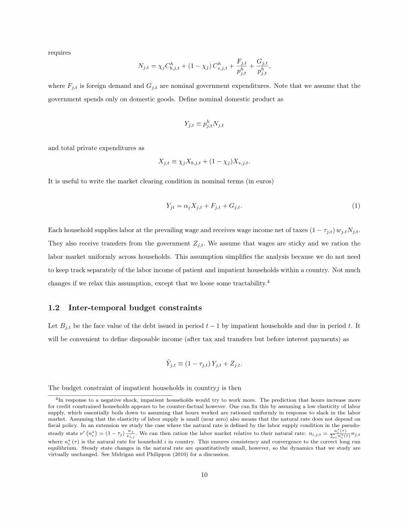
Figures (3), (4), (5) and (6) illustrate the impact of shocks to household debt (bhj,t), public spending (gj,t),

interest rates (rj,t) and foreign demand (fj,t).8

In Figure 3, an increase in household debt generates a boom in spending by impatient households,

employment and imports. Public debt falls but the net foreign asset position deteriorates. A fiscal expansion

(Figure 4) has qualitatively similar effects except that public debt increases. The multiplier for household

debt and government spending are increasing functions of αi and χi. A higher share of impatient agents in

the economy implies that an increase in disposable income has a larger impact on aggregate expenditures.

A higher share of spending on domestic goods reduces leakage through imports. Remember that patient

agents expenditures do not react to private or public debt changes.

An increase in interest rates (Figure 5) is very different because it induces patient households to save

more so it reduces their expenditures and generates a recession (fall in nominal GDP and in employment)

that obliges impatient households to reduce their spending. Imports fall and the net foreign asset position

improves. Because of lower tax revenues, the recession increases public debt. Finally, in Figure 6, an increase

in foreign demand permanently increases nominal GDP which induces patient households to increase their

saving. Spending of both patient and impatient households increase. The net foreign asset position improves.

Public debt falls because of higher tax revenues.7To be clear, this means that savers in our model anticipate spreads to last for one year. When we see in the data that

spreads remain high for 2 years in row, as in 2011 and 2012 for several countries, we interpret this as two negative shocks, whichseems consistent with the narrative of the crisis. For instance, concerns with bank liquidity created spreads in 2010. The ECBreacted by providing liquidity. But the relief was temporary because soon after investors became worried about sovereign riskand exit. Again, it took about a year for policy makers to find an appropriate response. We have also performed robustnesschecks to make sure that our results are not biased by this assumption (assuming for instance that investors anticipate spreadsto last for 2 years).

8For these impulse response functions, we use the following parameters: α = 0.75, χ = 0.5, r = 0.05, κ = 0.2, τ = 0.4. Prices,wages and employment are normalized to unity at time t = 0. The debt to income ratio is set at 60% for impatient householdsat time t = 0, so that the household debt to income ratio is 30%. The government debt to GDP ratio is set at 50% and the netforeign asset position over GDP is set at zero at time t = 0. The shock is a 20% increase of the variable at t = 1.

15

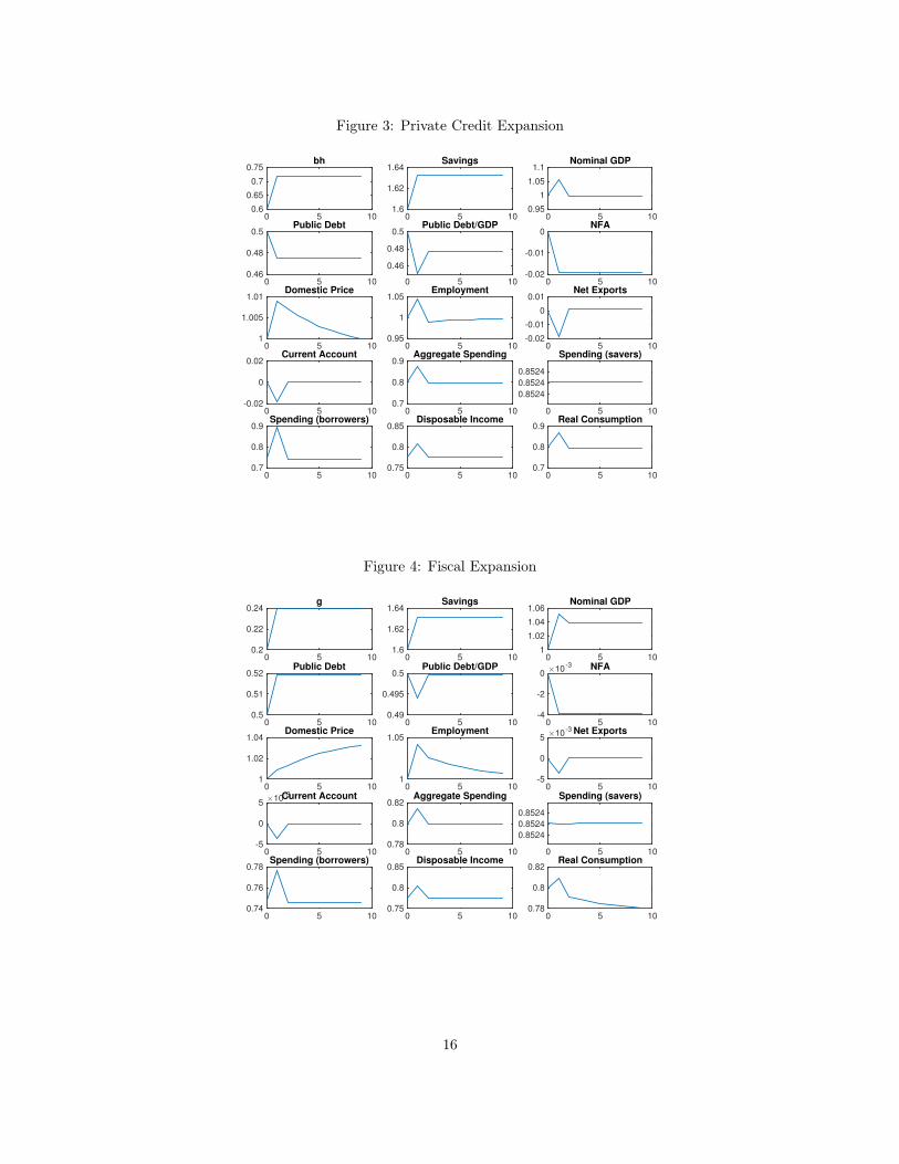
Figure 3: Private Credit Expansion

0 5 100.6

0.65

0.7

0.75bh

0 5 101.6

1.62

1.64Savings

0 5 100.95

1

1.05

1.1Nominal GDP

0 5 100.46

0.48

0.5Public Debt

0 5 10

0.46

0.48

0.5Public Debt/GDP

0 5 10-0.02

-0.01

0NFA

0 5 101

1.005

1.01Domestic Price

0 5 100.95

1

1.05Employment

0 5 10-0.02

-0.01

0

0.01Net Exports

0 5 10-0.02

0

0.02Current Account

0 5 100.7

0.8

0.9Aggregate Spending

0 5 10

0.8524

0.8524

0.8524

Spending (savers)

0 5 100.7

0.8

0.9Spending (borrowers)

0 5 100.75

0.8

0.85Disposable Income

0 5 100.7

0.8

0.9Real Consumption

Figure 4: Fiscal Expansion

0 5 100.2

0.22

0.24g

0 5 101.6

1.62

1.64Savings

0 5 101

1.02

1.04

1.06Nominal GDP

0 5 100.5

0.51

0.52Public Debt

0 5 100.49

0.495

0.5Public Debt/GDP

0 5 10

×10-3

-4

-2

0NFA

0 5 101

1.02

1.04Domestic Price

0 5 101

1.05Employment

0 5 10

×10-3

-5

0

5Net Exports

0 5 10

×10-3

-5

0

5Current Account

0 5 100.78

0.8

0.82Aggregate Spending

0 5 10

0.8524

0.8524

0.8524

Spending (savers)

0 5 100.74

0.76

0.78Spending (borrowers)

0 5 100.75

0.8

0.85Disposable Income

0 5 100.78

0.8

0.82Real Consumption

16

Figure 5: Interest rate shock

0 5 100.05

0.055

0.06rates

0 5 101.6

1.62

1.64Savings

0 5 100.98

1

1.02Nominal GDP

0 5 100.5

0.51

0.52Public Debt

0 5 100.5

0.51

0.52Public Debt/GDP

0 5 100

0.005

0.01NFA

0 5 100.996

0.998

1Domestic Price

0 5 100.98

1

1.02Employment

0 5 10-0.01

0

0.01Net Exports

0 5 10

×10-3

0

5

10Current Account

0 5 100.75

0.8

0.85Aggregate Spending

0 5 100.82

0.84

0.86Spending (savers)

0 5 100.73

0.74

0.75Spending (borrowers)

0 5 100.76

0.77

0.78Disposable Income

0 5 100.78

0.8

0.82Real Consumption

Figure 6: Foreign demand shock

0 5 100.2

0.22

0.24foreign

0 5 101.5

1.55

1.6Savings

0 5 101

1.1

1.2Nominal GDP

0 5 100.4

0.45

0.5Public Debt

0 5 100.3

0.4

0.5Public Debt/GDP

0 5 100

0.01

0.02NFA

0 5 101

1.1

1.2Domestic Price

0 5 101

1.1

1.2Employment

0 5 10-0.02

0

0.02Net Exports

0 5 10

×10-3

0

10

20Current Account

0 5 100.8

0.9

1Aggregate Spending

0 5 100.8

1

1.2Spending (savers)

0 5 100.6

0.8

1Spending (borrowers)

0 5 100.6

0.8

1Disposable Income

0 5 100.8

0.9

1Real Consumption

17

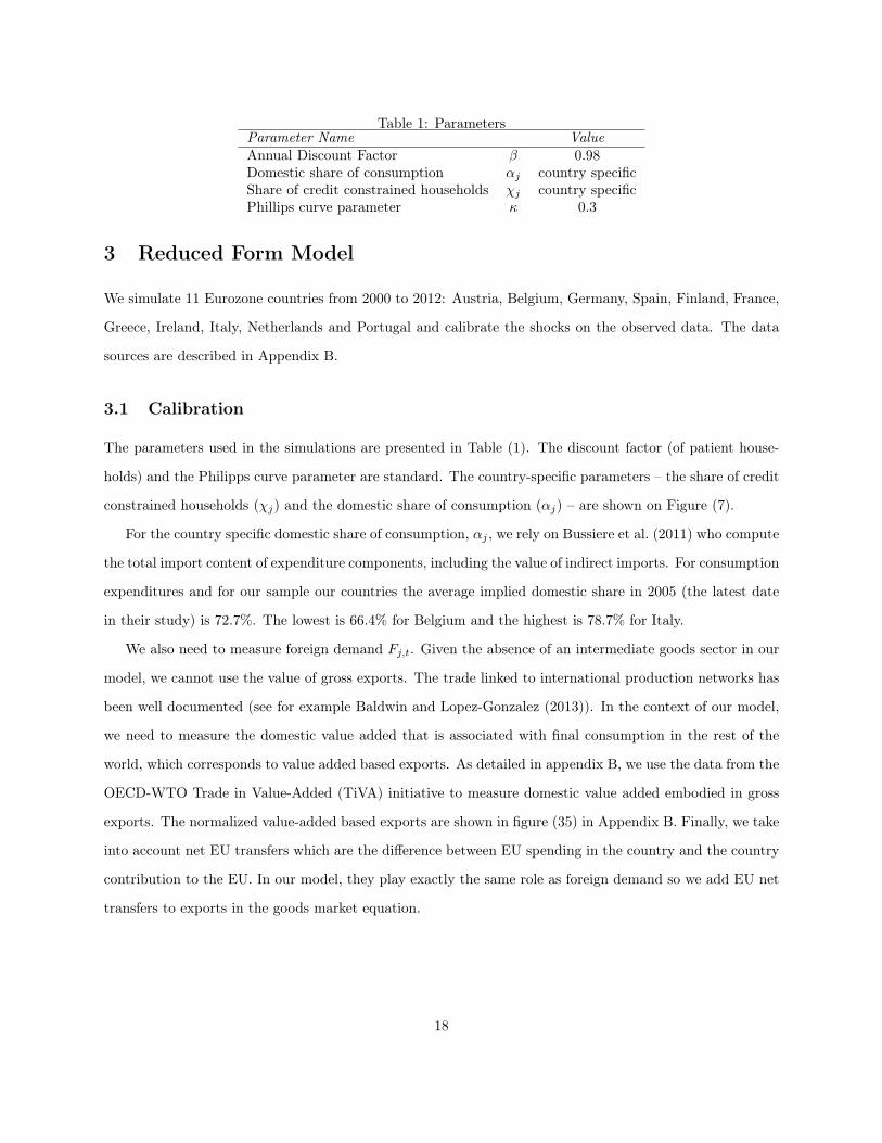
Table 1: ParametersParameter Name ValueAnnual Discount Factor β 0.98Domestic share of consumption αj country specificShare of credit constrained households χj country specificPhillips curve parameter κ 0.3

3 Reduced Form Model

We simulate 11 Eurozone countries from 2000 to 2012: Austria, Belgium, Germany, Spain, Finland, France,

Greece, Ireland, Italy, Netherlands and Portugal and calibrate the shocks on the observed data. The data

sources are described in Appendix B.

3.1 Calibration

The parameters used in the simulations are presented in Table (1). The discount factor (of patient house-

holds) and the Philipps curve parameter are standard. The country-specific parameters – the share of credit

constrained households (χj) and the domestic share of consumption (αj) – are shown on Figure (7).

For the country specific domestic share of consumption, αj , we rely on Bussiere et al. (2011) who compute

the total import content of expenditure components, including the value of indirect imports. For consumption

expenditures and for our sample our countries the average implied domestic share in 2005 (the latest date

in their study) is 72.7%. The lowest is 66.4% for Belgium and the highest is 78.7% for Italy.

We also need to measure foreign demand Fj,t. Given the absence of an intermediate goods sector in our

model, we cannot use the value of gross exports. The trade linked to international production networks has

been well documented (see for example Baldwin and Lopez-Gonzalez (2013)). In the context of our model,

we need to measure the domestic value added that is associated with final consumption in the rest of the

world, which corresponds to value added based exports. As detailed in appendix B, we use the data from the

OECD-WTO Trade in Value-Added (TiVA) initiative to measure domestic value added embodied in gross

exports. The normalized value-added based exports are shown in figure (35) in Appendix B. Finally, we take

into account net EU transfers which are the difference between EU spending in the country and the country

contribution to the EU. In our model, they play exactly the same role as foreign demand so we add EU net

transfers to exports in the goods market equation.

18

Figure 7: Share of credit constrained households (χj) and domestic share of consumption (αj)

AUT

BEL

DEU

ESP

FIN

FRA

GRE

IRL

ITA

NLD

PRT

.6.6

5.7

.75

.8alp

ha

.3 .4 .5 .6 .7chi

Share of Constrained Households For the country specific share of credit constrained borrowers, χj , we

use a measure by Mendicino (2014) based on the Eurosystem Household Finance and Consumption Survey

(HFCS).9 For each country, Mendicino (2014) computes the fraction of household with liquid assets below

two months of total households gross income to approximate the share of credit constrained households. The

average for our set of countries is 48% with a maximum of 64.8% for Greece and a minimum of 34.7% for

Austria. Ireland did not participate in the survey so for this country we use the average of the eurozone.

Note that bhj,t in the model is debt per impatient household so the counterpart to the empirical measure of

aggregate debt is χjbhj,t.

Cost of Fund The cost of fund ρj,t enters the Euler equation of unconstrained agents. It should represent

at the same time the expected return of savers, the borrowing cost of unconstrained borrowers, and the

funding cost of firms. The issue is that we only observe some interest rates, not expected returns or funding

costs. We use several interest rates: (i) yields on 10-year government bonds; (ii) loans rates for SMEs;

(iii) deposit rates; (iv) wholesale bank funding costs. In all cases we compute the difference between the

rate in country j and the median of the Eurozone in year t. Sovereign spreads are not expected returns,

however, because they include expected credit losses. On the other hand, we know from a huge literature9The survey took place in 2010. In Greece and Spain, the data were collected in 2009 and 2008-09 respectively. This

survey has been used recently by Kaplan et al. (2014) to quantify the share of hand-to-month households. They define theseas consumers who spend all of their available resources in every pay-period, and hence do not carry any wealth across periods.They argue that measuring this behavior using data on net worth (as consistent with heterogeneous-agent macroeconomicmodels ) is misleading because this misses what they call the wealthy hand-to-mouth households. These are households whohold sizable amounts of wealth in illiquid assets (such as housing or retirement accounts), but very little or no liquid wealth,and therefore consume all of their disposable income every period. They define hand-to-mouth consumers as those householdsin the survey whose average balances of liquid wealth are positive but equal to or less than half their earnings.

19

in finance that credit spreads create significant differences in funding costs. This is the basic point of all

models with distress costs, agency costs, debt overhang, safety premia, etc. For bank-dependent borrowers,

the funding costs of banks and the opportunity cost of lending are obviously critical. Both are tightly linked

to sovereign spreads. Banks almost never borrow more cheaply than their own sovereign, and debt overhang

in the banking sector makes it more attractive to invest in the debt of home sovereign.10 This suggests that

one could think of ρ as the common component of rates (i)-(iv). But in practice we are constrained by data

availability. The only rates consistently available for all years and all countries are the sovereign yield. We

find that the following transformation of the sovereign yields makes them comparable to the other rates:

ρ = ∆I∆<1% +∆− 1%

2I∆∈[1%,3%] +

∆− 3%

4I∆∈[3%,5%] +

∆− 5%

8I∆>5%,

where ∆ is the deviation of the yield from the Eurozone median and ρ is our measure of spreads in funding

costs. What this means is that, for the first 100 basis points, we treat the spread as a funding cost. This

is consistent with estimates of flight to quality towards German assets and liquidity risk premia. Then we

divide the spread by two, etc. Above 500 basis points, we assume that only 1/8th of the spread represent

funding costs. This filter creates funding costs that are comparable to the (limited) data we have on deposit

rates, SME rates, and wholesale funding costs. Our results are robust as long as we trim the large spreads,

otherwise the drop in consumption by savers is simply too large to be consistent with the data. Both the 10

year government bond spreads (the deviation of the yield from the Eurozone median) and ρ as measured in

the equation above are shown in figure (36) in appendix B.

Scaling In order to map the observed data into the model we scale the data in a manner consistent with

equation (12). We construct the following benchmark level of nominal GDP for country j at time t:

Yj,t ≡Yj,t0Nj,t0

Nt0Yt0

YtNtNj,t,

where t0 is the base year (2002 in our simulations), Y is GDP, N is population, and Yt and Nt denote

aggregate for the Eurozone. In words, the benchmark is the nominal GDP the country would have if it had

the same per-capita growth rate as the eurozone together with its actual population growth. The key point

is that the only country level time-varying variable that we take as exogenous is population growth. We10In the limit of a model à la Myers (1977), the bank may end up treating the entire yield as an expected return because it

only cares about the non-default state. See Philippon and Schnabl (2009) for a discussion of debt overhang.

20

than scale all our variables in euros by the benchmark GDP. For GDP itself, we define

yj,t ≡Yj,t

Yj,t

which is one in the base year. For sovereign debt, we define

bgj,t ≡Bgj,t

Yj,t,

which is the actual debt to GDP ratio for the base year, but then tracks the level of debt, as in the

model. This is important when we consider deleveraging. With large fiscal multipliers, a reduction in debt

might leave the debt to GDP ratio unchanged in the short run. Ratios might give a very misleading view of

deleveraging efforts. The normalized data for private and sovereign debt are shown in figure (33) in Appendix

B. Normalized public spending and transfers are shown (34). Note also that government spending is adjusted

for expenditures on bank recapitalization. For unit labor costs, we scale by the average unit labor cost in

the eurozone. For employment we use employment per capita and we take the deviation from the base year.

3.2 Reduced Form Simulations

In our reduced form simulations, we take as given the observed series for private debt (bhj,t), fiscal policy

(gj,t, zj,t, τj) and interest rate spreads (ρj,t). The reduced form model < is a mapping

< :(bhj,t, gj,t, zj,t, ρj,t

)−→

(bgj,t, yj,t, nj,t, pj,t, ej,t, ..

)(14)

The scaled data on observed shocks that serve to feed the model for each country are shown in figures (33),

(34), (36) and (35) in Appendix B. For each country, we simulate the path between 2001 and 2012 of nominal

GDP yj,t, employment nj,t, wages wj,t, net exports ej,t and public debt bgj,t.

It is important to emphasize that there is no degree of freedom in our simulations. There is no parameter

which is set to match any moment in the data. The model is entirely constrained by observable micro

estimates and by equilibrium conditions. The only parameter that we can adjust is the slope of the Phillips

curve κ but it does not affect the nominal GDP in euros, it only pins down the allocation of nominal GDP

between prices (unit labor cost) and quantities (employment).

Figures (8), (9), (10) show the simulated and observed nominal GDP, net exports and employment. The

reduced form model reproduces very well the cross sectional dynamics in the euro zone for nominal GDP

21

and net exports. In particular, it replicates well the boom and bust dynamics on nominal GDP and the

current account reversal for the crisis hit countries. For employment, the model does also well for the crisis

countries and for countries that were hit less severely.

Figure 8: Reduced Form Model, Nominal GDP

2001 2004 2008 2012

0.9

1

1.1

1.2

AUT

2001 2004 2008 2012

0.9

1

1.1

1.2

BEL

2001 2004 2008 2012

0.9

1

1.1

1.2

DEU

2001 2004 2008 2012

0.9

1

1.1

1.2

ESP

2001 2004 2008 2012

0.9

1

1.1

1.2

FIN

2001 2004 2008 2012

0.9

1

1.1

1.2

FRA

2001 2004 2008 2012

0.9

1

1.1

1.2

GRE

2001 2004 2008 2012

0.9

1

1.1

1.2

IRL

2001 2004 2008 2012

0.9

1

1.1

1.2

ITA

2001 2004 2008 2012

0.9

1

1.1

1.2

NLD

year2001 2004 2008 2012

0.9

1

1.1

1.2

PRT

data

reduced form model

22

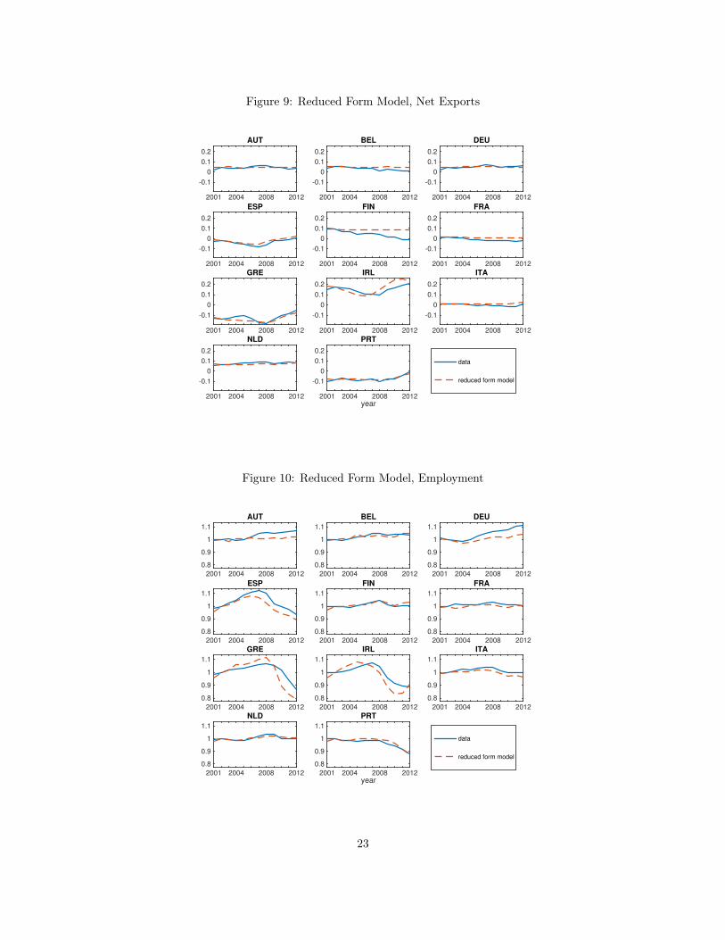
Figure 9: Reduced Form Model, Net Exports

2001 2004 2008 2012

-0.1

0

0.1

0.2

AUT

2001 2004 2008 2012

-0.1

0

0.1

0.2

BEL

2001 2004 2008 2012

-0.1

0

0.1

0.2

DEU

2001 2004 2008 2012

-0.1

0

0.1

0.2

ESP

2001 2004 2008 2012

-0.1

0

0.1

0.2

FIN

2001 2004 2008 2012

-0.1

0

0.1

0.2

FRA

2001 2004 2008 2012

-0.1

0

0.1

0.2

GRE

2001 2004 2008 2012

-0.1

0

0.1

0.2

IRL

2001 2004 2008 2012

-0.1

0

0.1

0.2

ITA

2001 2004 2008 2012

-0.1

0

0.1

0.2

NLD

year2001 2004 2008 2012

-0.1

0

0.1

0.2

PRT

data

reduced form model

Figure 10: Reduced Form Model, Employment

2001 2004 2008 2012

0.8

0.9

1

1.1

AUT

2001 2004 2008 2012

0.8

0.9

1

1.1

BEL

2001 2004 2008 2012

0.8

0.9

1

1.1

DEU

2001 2004 2008 2012

0.8

0.9

1

1.1

ESP

2001 2004 2008 2012

0.8

0.9

1

1.1

FIN

2001 2004 2008 2012

0.8

0.9

1

1.1

FRA

2001 2004 2008 2012

0.8

0.9

1

1.1

GRE

2001 2004 2008 2012

0.8

0.9

1

1.1

IRL

2001 2004 2008 2012

0.8

0.9

1

1.1

ITA

2001 2004 2008 2012

0.8

0.9

1

1.1

NLD

year2001 2004 2008 2012

0.8

0.9

1

1.1

PRT

data

reduced form model

23

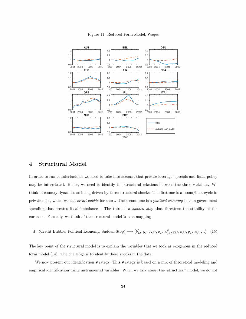
Figure 11: Reduced Form Model, Wages

2001 2004 2008 20120.9

1

1.1

1.2

AUT

2001 2004 2008 20120.9

1

1.1

1.2

BEL

2001 2004 2008 20120.9

1

1.1

1.2

DEU

2001 2004 2008 20120.9

1

1.1

1.2

ESP

2001 2004 2008 20120.9

1

1.1

1.2

FIN

2001 2004 2008 20120.9

1

1.1

1.2

FRA

2001 2004 2008 20120.9

1

1.1

1.2

GRE

2001 2004 2008 20120.9

1

1.1

1.2

IRL

2001 2004 2008 20120.9

1

1.1

1.2

ITA

2001 2004 2008 20120.9

1

1.1

1.2

NLD

year2001 2004 2008 2012

0.9

1

1.1

1.2

PRT

data

reduced form model

4 Structural Model

In order to run counterfactuals we need to take into account that private leverage, spreads and fiscal policy

may be interrelated. Hence, we need to identify the structural relations between the three variables. We

think of country dynamics as being driven by three structural shocks. The first one is a boom/bust cycle in

private debt, which we call credit bubble for short. The second one is a political economy bias in government

spending that creates fiscal imbalances. The third is a sudden stop that threatens the stability of the

eurozone. Formally, we think of the structural model = as a mapping

= : (Credit Bubble, Political Economy, Sudden Stop) −→(bhj,t, gj,t, zj,t, ρj,t; b

gj,t, yj,t, nj,t, pj,t, ej,t, ..

)(15)

The key point of the structural model is to explain the variables that we took as exogenous in the reduced

form model (14). The challenge is to identify these shocks in the data.

We now present our identification strategy. This strategy is based on a mix of theoretical modeling and

empirical identification using instrumental variables. When we talk about the “structural” model, we do not

24

mean that we have provided micro-foundations for every detail of the model. Given the range of data and

economic forces that we need to capture, this is not even remotely possible. But we mean that, either there

is an explicit theoretical equation, or there is an identified empirical equation that allows us to capture the

influence of one variable on the others.

4.1 Using the U.S. to Identify Private Debt Dynamics

We use the US as a control group to estimate leverage dynamics without sudden stops. More precisely, we

estimate the following model for deleveraging in a panel of U.S. states

bh,USj,t =

3∑k=1

αUSk bh,USj,t−k + εj,t

for t = 2008, .., 2012, j = 1, ..52, and bhj,t is household debt detrended exactly as in the Eurozone. The idea

is that these private leverage bubbles reflected various global and financial factors: low real rates, financial

innovations, regulatory arbitrage of the Basel rules by banks, real estate bubbles, etc. To a large extent

these forces were present both in Europe and in the US. The difference of course is that there was no sudden

stops within the US. Hence, we interpret the US experience as representative of a deleveraging outcome in

a monetary union without sudden stops.11

We then take the estimated coefficients αUSk and use them to construct predicted deleveraging in Eurozone

countries:

bhj,t =

K∑k=1

αUSk bh,j,t−k

for t = 2008, .., 2012 and j = 1..11. Figure 12 illustrates the results for California and Ireland. The model

predicts a somewhat slower deleveraging in Ireland than actually happened. This is also the case for other

countries that experienced a sudden stop.

We now posit the following structural equations. Private leverage in euro zone countries is given by:

bhj,t+1 = λh0 + bhj,t + λρ,hρj,t. (16)

Private leverage is equal to the prediction from the US experience plus the impact of the spread. The first

element of the private leverage, bhj,t, is interpreted as an exogenous shock. The second element, the impact

of the spread, is endogenous and is meant to capture various transmission channels. An obvious one is11We discuss differences in local fiscal policy in the Appendix.

25

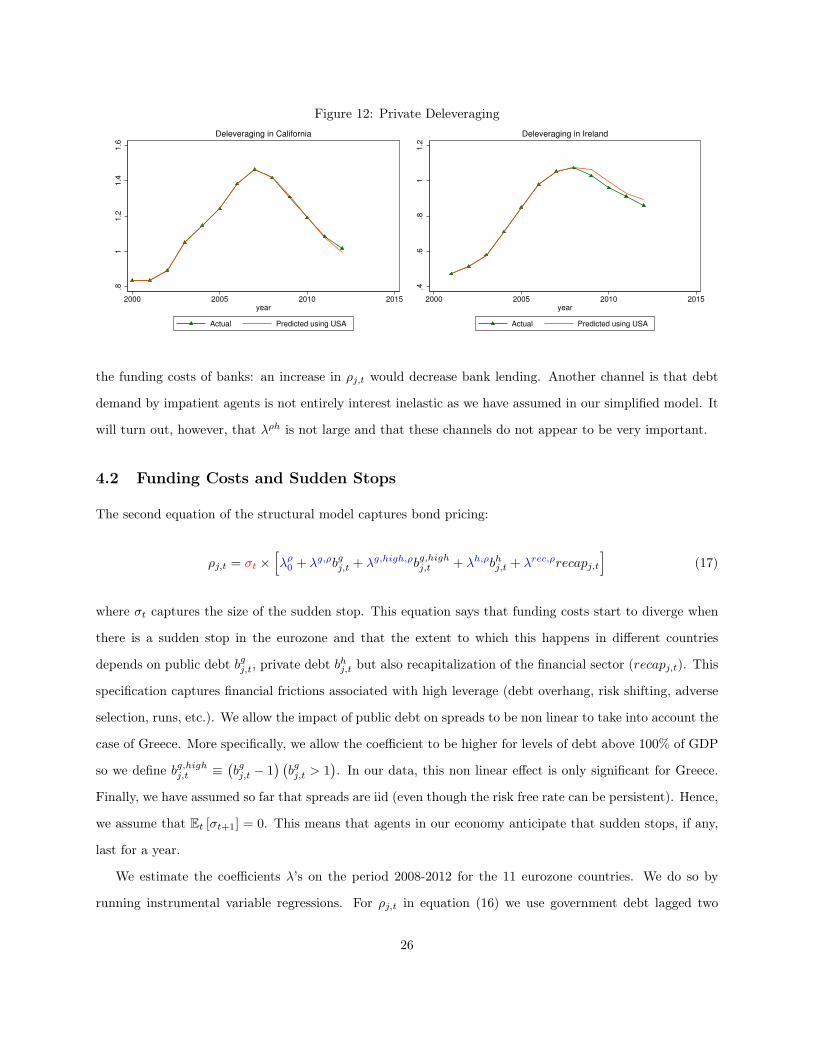
Figure 12: Private Deleveraging.8

11.2

1.4

1.6

2000 2005 2010 2015year

Actual Predicted using USA

Deleveraging in California

.4.6

.81

1.2

2000 2005 2010 2015year

Actual Predicted using USA

Deleveraging in Ireland

the funding costs of banks: an increase in ρj,t would decrease bank lending. Another channel is that debt

demand by impatient agents is not entirely interest inelastic as we have assumed in our simplified model. It

will turn out, however, that λρh is not large and that these channels do not appear to be very important.

4.2 Funding Costs and Sudden Stops

The second equation of the structural model captures bond pricing:

ρj,t = σt ×[λρ0 + λg,ρbgj,t + λg,high,ρbg,highj,t + λh,ρbhj,t + λrec,ρrecapj,t

](17)

where σt captures the size of the sudden stop. This equation says that funding costs start to diverge when

there is a sudden stop in the eurozone and that the extent to which this happens in different countries

depends on public debt bgj,t, private debt bhj,t but also recapitalization of the financial sector (recapj,t). This

specification captures financial frictions associated with high leverage (debt overhang, risk shifting, adverse

selection, runs, etc.). We allow the impact of public debt on spreads to be non linear to take into account the

case of Greece. More specifically, we allow the coefficient to be higher for levels of debt above 100% of GDP

so we define bg,highj,t ≡(bgj,t − 1

) (bgj,t > 1

). In our data, this non linear effect is only significant for Greece.

Finally, we have assumed so far that spreads are iid (even though the risk free rate can be persistent). Hence,

we assume that Et [σt+1] = 0. This means that agents in our economy anticipate that sudden stops, if any,

last for a year.

We estimate the coefficients λ’s on the period 2008-2012 for the 11 eurozone countries. We do so by

running instrumental variable regressions. For ρj,t in equation (16) we use government debt lagged two

26

and three years as instruments. For government and private debt bgj,t and bhj,t, in equation (17), we use

as instruments government debt levels (bgj,t and bg,highj,t ) lagged three years, the exogenous component of

private debt (and its lag) predicted by the US experience bhj,t. To capture the possibility and the size of a

sudden stop in the eurozone, we measure the coefficient σt as the divergence in spreads across the eurozone

countries. More precisely, for each year, σt equals the mean of the absolute value of spreads in the eurozone.

As expected, it is low and close to zero up to 2007 and starts increasing in 2008 with a maximum in 2012.

The estimated coefficients, which we will use in our simulations, are shown in Table (2):

Table 2: Coefficients Estimated with Instrumental Variables.λh0 λρ,h λρ0 λg,ρ λh,ρ λrec,ρ

−0.005 −1.2 −2.3 2 1.2 15(0.002) (0.184) (0.16) (0.4) (0.3) (3)

Note: standard errors in parenthesis.

For the non linear effect of public debt on spreads, we set λg,high,ρ = 1 since it gives the best fit for

Greece.

4.3 Fiscal Policy

Our last task is to specify a fiscal policy function for the different governments. We assume that the

government seeks to stabilize employment but is constrained by its costs of funds. The funding constraint is

measured by the (lagged) spread ρj,t−1 and is only binding when the spread is positive.12 Hence, the policy

rule for government spending, with parameters γn and γρ, is given by:

gj,t = gj,t + γn (nj,t − n) + γρρj,t−1 if ρj,t−1 > 0, (18)

gj,t = gj,t + γn (nj,t − n) if ρj,t−1 < 0,

where gj,t is a country specific drift which is linearly increasing until 2008 and decreasing afterwards:

gj,t = gj,0 + δgj (min(t, t1)− t0)− δgj max (t− t1, 0) (19)

with t0 = 2002 and t1 = 2008. Hence, δgj represents the average “excess” annual spending growth rate

during the boom years. We interpret this drift as a political bias in spending decisions that is reversed after12We use the t-1 spread simply because it fits better, which probably reflects implementation lags in fiscal policy. This is not

related to the identification of the model and our results are not sensitive to this detail.

27

2008. The change in political bias might come from new fiscal rules agreed at the EU level, from explicit

requirements for countries in a program, or more broadly from a shift in attitudes and beliefs about fiscal

responsibility.13 What matters for us, however, is that countries displayed different level of spending bias

during the boom years, and we want to analyze to what extent this spending drift during the boom years

may have contributed to the euro crisis. The same structural equations apply to transfers zj,t with specific

values for zj,0 and δzj .

We now focus on the four countries that were most harshly hit by the crisis, namely Spain, Greece,

Ireland and Portugal. We choose our parameters in the policy rule γn andγρ and the spending and transfer

drift coefficients δgj and δzj such that the model reproduces as best as possible the dynamics of observed

nominal GDP, public debt, employment and spreads.

This leads us to choose the parameters given in Table (3) and (4) :

Table 3: Fiscal policy coefficientsγn γρ

−0.5 −3

Table 4: Fiscal policy drifts: government spending and transfersδgj δzj

Spain Greece Ireland Portugal Spain Greece Ireland Portugal1.5% 1% 0.5% 0% 1.0% 3.0% 2.0% 0.5%

Note that the spending and transfers drift necessary to reproduce the debt dynamics is (not surprisingly)

much larger in Greece than in the other periphery countries. It is intermediate and similar in Ireland and

Spain and very small in Portugal.

We also need to take into account the specific case of Greece which benefited in 2012 from a debt relief

that reduced its public debt by around 50% of GDP and in 2011, from a reduction in interest rates and an

extension in the repayment period for the EU and IMF rescue package. We do this by adding 10% of GDP

and 40% of GDP to government revenues in 2011 and 2012. This allows to better replicate the Greek public

debt in 2012.13The fact that it is reversed is not very important for our results. We could assume that gj,t stays constant after t1 and our

simulations would be similar. In fact, our counter-factual results would be stronger since the model would then choose a largerγρ to fit the data. But this can create issues of debt sustainability if we simulate the model beyond 2012 and we assume thatthe spreads normalize. In practice we also see that governments are trying to reverse some of the spending decisions they madeduring the boom years.

28

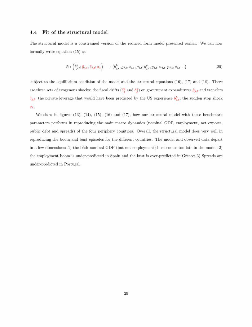
4.4 Fit of the structural model

The structural model is a constrained version of the reduced form model presented earlier. We can now

formally write equation (15) as

= :(bhj,t; gj,t, zj,t;σt

)−→

(bhj,t, gj,t, zj,t, ρj,t; b

gj,t, yj,t, nj,t, pj,t, ej,t, ..

)(20)

subject to the equilibrium condition of the model and the structural equations (16), (17) and (18). There

are three sets of exogenous shocks: the fiscal drifts (δgj and δzj ) on government expenditures gj,t and transfers

zj,t, the private leverage that would have been predicted by the US experience bhj,t, the sudden stop shock

σt.

We show in figures (13), (14), (15), (16) and (17), how our structural model with these benchmark

parameters performs in reproducing the main macro dynamics (nominal GDP, employment, net exports,

public debt and spreads) of the four periphery countries. Overall, the structural model does very well in

reproducing the boom and bust episodes for the different countries. The model and observed data depart

in a few dimensions: 1) the Irish nominal GDP (but not employment) bust comes too late in the model; 2)

the employment boom is under-predicted in Spain and the bust is over-predicted in Greece; 3) Spreads are

under-predicted in Portugal.

29

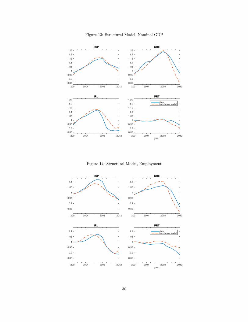
Figure 13: Structural Model, Nominal GDP

2001 2004 2008 2012

0.85

0.9

0.95

1

1.05

1.1

1.15

1.2

1.25

ESP

2001 2004 2008 2012

0.85

0.9

0.95

1

1.05

1.1

1.15

1.2

1.25

GRE

2001 2004 2008 2012

0.85

0.9

0.95

1

1.05

1.1

1.15

1.2

1.25

IRL

year2001 2004 2008 2012

0.85

0.9

0.95

1

1.05

1.1

1.15

1.2

1.25

PRT

databenchmark model

Figure 14: Structural Model, Employment

2001 2004 2008 2012

0.85

0.9

0.95

1

1.05

1.1

ESP

2001 2004 2008 2012

0.85

0.9

0.95

1

1.05

1.1

GRE

2001 2004 2008 2012

0.85

0.9

0.95

1

1.05

1.1

IRL

year2001 2004 2008 2012

0.85

0.9

0.95

1

1.05

1.1

PRT

databenchmark model

30

Figure 15: Structural Model, Net Exports

2001 2004 2008 2012

-0.15

-0.1

-0.05

0

0.05

0.1

0.15

0.2

0.25

ESP

2001 2004 2008 2012

-0.15

-0.1

-0.05

0

0.05

0.1

0.15

0.2

0.25

GRE

2001 2004 2008 2012

-0.15

-0.1

-0.05

0

0.05

0.1

0.15

0.2

0.25

IRL

year2001 2004 2008 2012

-0.15

-0.1

-0.05

0

0.05

0.1

0.15

0.2

0.25

PRT

databenchmark model

31

Figure 16: Structural Model, Government Debt

32

Figure 17: Structural Model, Funding Costs

2001 2004 2008 2012

-0.02

-0.01

0

0.01

0.02

0.03

0.04

0.05

0.06

ESP

2001 2004 2008 2012

-0.02

-0.01

0

0.01

0.02

0.03

0.04

0.05

0.06

GRE

2001 2004 2008 2012

-0.02

-0.01

0

0.01

0.02

0.03

0.04

0.05

0.06

IRL

year2001 2004 2008 2012

-0.02

-0.01

0

0.01

0.02

0.03

0.04

0.05

0.06

PRT

databenchmark model

5 Counterfactual experiments

We now present our main structural experiments. The goal is to provide counter-factual simulations of what

would have happened to the four countries (Greece, Spain, Ireland and Portugal) that were most affected

by the crisis had they followed a different set of policies. We consider four counterfactuals:

• fiscal policy: what would have happened if those countries had pursued a more conservative fiscal

policy before 2008?

• macro-prudential policies: what would have happened if they had limited the growth of household

debt?

• monetary policy: what would have happened if the “whatever it takes” commitment by the ECB had

been announced in 2008 rather than in 2012?

• fiscal devaluation: what would have happened if they had been engineered a fiscal devaluation and

reduce export prices?

33

For the counterfactual experiments, we use the structural equations (16) and (17) for private debt and spreads

respectively and the fiscal policy rule (18). We use the same coefficient estimates from the instrumental

variables regression (shown in Table 2) for the structural equations for private debt and spreads and the

policy rule (18). For all counterfactual experiments, we compare on the same graph the data and the

counterfactual experiment which we define as: structural model with counterfactual parameters + (data -

structural model with benchmark parameters) so that we take into account that the structural model with

benchmark parameters does not perfectly reproduce the data although we have seen that it does so very

well. The simulation generates cross sectional time series for public debt, private debt, employment, nominal

GDP, net exports and spreads on the period 2001-2012, using debt in 2000 as an initial point.

5.1 Counterfactual with a more conservative fiscal policy in the boom

How would countries have fared if they had followed more conservative fiscal policies during the boom? We

answer this question by removing the fiscal drift bias in the fiscal rule (18). Hence, we set δgj and δzj equal to

zero for the four periphery countries. For Spain, Ireland and Portugal all the other benchmark parameters

are left unchanged. For Greece, we need to deal with the debt relief issue. Given that the counterfactual

conservative fiscal policy generates debt to GDP ratios below 120%, we assume that debt relief would not

have taken place. Hence, for Greece the counterfactual is the combination of a more conservative fiscal policy

but also the elimination of a transfer of around 50% of nominal GDP in 2011-2012.

The elimination of the fiscal drift dramatically changes the public debt accumulation for Greece, Ireland

and Spain but less so in Portugal which is not surprising given that our exercise suggests that the fiscal drift

was very large in Greece, large in Ireland and Spain but small in Portugal. This can be seen in figure (18)

where counterfactual public debt in Greece is stabilized in 2011 close to its level in 2001. Ireland would

have eliminated all public debt just before the bust and in Spain it would have been reduced to around 26%

of GDP. Hence, fiscal policy, once the fiscal drifts are removed, becomes more conservative but also more

countercyclical. This large change in the public debt in turns reduces spreads during the sudden stop in

Greece, Ireland and Spain but very little in Portugal as shown in figure (19). Lower spreads allow fiscal policy

to be less constrained during the bust which explains part of the increase in debt in the periphery countries

in the latest years. The counterfactual conservative fiscal policy in Greece is very successful in stabilizing

employment as shown in figure (20). Remember that this more conservative fiscal policy in Greece also

means that this country does not benefit from the debt relief at the end of the period. The counterfactual

conservative fiscal policies in the boom - which allow for less fiscal austerity in the bust - in Spain and

34

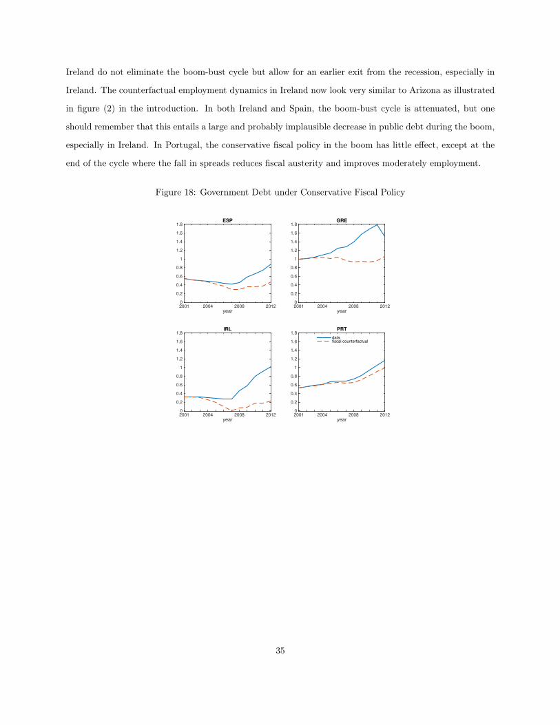
Ireland do not eliminate the boom-bust cycle but allow for an earlier exit from the recession, especially in

Ireland. The counterfactual employment dynamics in Ireland now look very similar to Arizona as illustrated

in figure (2) in the introduction. In both Ireland and Spain, the boom-bust cycle is attenuated, but one

should remember that this entails a large and probably implausible decrease in public debt during the boom,

especially in Ireland. In Portugal, the conservative fiscal policy in the boom has little effect, except at the

end of the cycle where the fall in spreads reduces fiscal austerity and improves moderately employment.

Figure 18: Government Debt under Conservative Fiscal Policy

year2001 2004 2008 20120

0.2

0.4

0.6

0.8

1

1.2

1.4

1.6

1.8ESP

year2001 2004 2008 20120

0.2

0.4

0.6

0.8

1

1.2

1.4

1.6

1.8GRE

year2001 2004 2008 20120

0.2

0.4

0.6

0.8

1

1.2

1.4

1.6

1.8IRL

year2001 2004 2008 20120

0.2

0.4

0.6

0.8

1

1.2

1.4

1.6

1.8PRT

datafiscal counterfactual

35

Figure 19: Spreads under Conservative Fiscal Policy

year2001 2004 2008 2012

-0.02

-0.01

0

0.01

0.02

0.03

0.04

0.05

0.06

ESP

year2001 2004 2008 2012

-0.02

-0.01

0

0.01

0.02

0.03

0.04

0.05

0.06

GRE

year2001 2004 2008 2012

-0.02

-0.01

0

0.01

0.02

0.03

0.04

0.05

0.06

IRL

year2001 2004 2008 2012

-0.02

-0.01

0

0.01

0.02

0.03

0.04

0.05

0.06

PRT

datafiscal counterfactual

Figure 20: Employment under Conservative Fiscal Policy

year2001 2004 2008 2012

0.9

0.95

1

1.05

1.1

ESP

year2001 2004 2008 2012

0.9

0.95

1

1.05

1.1

GRE

year2001 2004 2008 2012

0.9

0.95

1

1.05

1.1

IRL

year2001 2004 2008 2012

0.9

0.95

1

1.05

1.1

PRT

datafiscal counterfactual

36

5.2 Counterfactual with macro-prudential policies in the boom

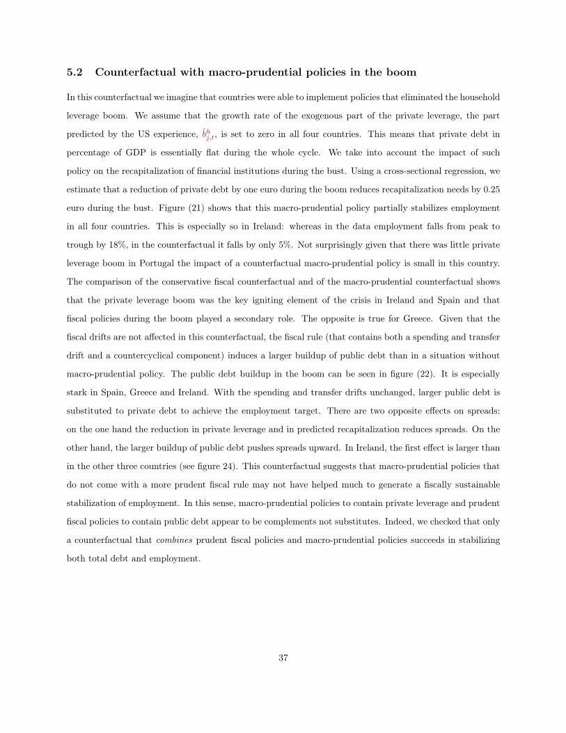
In this counterfactual we imagine that countries were able to implement policies that eliminated the household

leverage boom. We assume that the growth rate of the exogenous part of the private leverage, the part

predicted by the US experience, bhj,t, is set to zero in all four countries. This means that private debt in

percentage of GDP is essentially flat during the whole cycle. We take into account the impact of such

policy on the recapitalization of financial institutions during the bust. Using a cross-sectional regression, we

estimate that a reduction of private debt by one euro during the boom reduces recapitalization needs by 0.25

euro during the bust. Figure (21) shows that this macro-prudential policy partially stabilizes employment

in all four countries. This is especially so in Ireland: whereas in the data employment falls from peak to

trough by 18%, in the counterfactual it falls by only 5%. Not surprisingly given that there was little private

leverage boom in Portugal the impact of a counterfactual macro-prudential policy is small in this country.

The comparison of the conservative fiscal counterfactual and of the macro-prudential counterfactual shows

that the private leverage boom was the key igniting element of the crisis in Ireland and Spain and that

fiscal policies during the boom played a secondary role. The opposite is true for Greece. Given that the

fiscal drifts are not affected in this counterfactual, the fiscal rule (that contains both a spending and transfer

drift and a countercyclical component) induces a larger buildup of public debt than in a situation without

macro-prudential policy. The public debt buildup in the boom can be seen in figure (22). It is especially

stark in Spain, Greece and Ireland. With the spending and transfer drifts unchanged, larger public debt is

substituted to private debt to achieve the employment target. There are two opposite effects on spreads:

on the one hand the reduction in private leverage and in predicted recapitalization reduces spreads. On the

other hand, the larger buildup of public debt pushes spreads upward. In Ireland, the first effect is larger than

in the other three countries (see figure 24). This counterfactual suggests that macro-prudential policies that

do not come with a more prudent fiscal rule may not have helped much to generate a fiscally sustainable

stabilization of employment. In this sense, macro-prudential policies to contain private leverage and prudent

fiscal policies to contain public debt appear to be complements not substitutes. Indeed, we checked that only

a counterfactual that combines prudent fiscal policies and macro-prudential policies succeeds in stabilizing

both total debt and employment.

37

Figure 21: Employment with Macro-Prudential Policies

year2001 2004 2008 2012

0.9

0.95

1

1.05

1.1

ESP

year2001 2004 2008 2012

0.9

0.95

1

1.05

1.1

GRE

year2001 2004 2008 2012

0.9

0.95

1

1.05

1.1

IRL

year2001 2004 2008 2012

0.9

0.95

1

1.05

1.1

PRT

datamacroprudential counterfactual

Figure 22: Public debt with Macro-Prudential Policies

year2001 2004 2008 2012

0.4

0.6

0.8

1

1.2

1.4

1.6

1.8

2

ESP

year2001 2004 2008 2012

0.4

0.6

0.8

1

1.2

1.4

1.6

1.8

2

GRE

year2001 2004 2008 2012

0.4

0.6

0.8

1

1.2

1.4

1.6

1.8

2

IRL

year2001 2004 2008 2012

0.4

0.6

0.8

1

1.2

1.4

1.6

1.8

2

PRT

datamacroprudential counterfactual

38

Figure 23: Spreads with Macro-Prudential Policies

year2001 2004 2008 2012

-0.01

0

0.01

0.02

0.03

0.04

0.05

0.06

ESP

year2001 2004 2008 2012

-0.01

0

0.01

0.02

0.03

0.04

0.05

0.06

GRE

year2001 2004 2008 2012

-0.01

0

0.01

0.02

0.03

0.04

0.05

0.06

IRL

year2001 2004 2008 2012

-0.01

0

0.01

0.02

0.03

0.04

0.05

0.06

PRT

datamacroprudential counterfactual

5.3 Counterfactual with “whatever it takes” in 2008

In this counterfactual we ask the following question: what would have happened if the announcements of July

2012 (Mario Draghi’s declaration “Whatever it takes”) and September 2012 (the OMT program) that were

successful in reducing the risk of a euro breakup, the sudden stop and the spreads of the periphery countries

had come earlier. The experiment is to imagine that these actions were implemented and successful in 2008

rather than 2012. We assume that, starting in 2008, σt, the mean of the absolute value of spreads in the

eurozone, that enters the spread equation (17), is kept at its low 2007 level. This effectively eliminates the

sudden stop and the dramatic rise in spreads as illustrated in figure (24). This allows to reduce the cost of

borrowing constraint in the fiscal rule so that the countries can avoid fiscal austerity and stabilize employment

(see figure25). The employment dynamics of Ireland and Arizona (see figure 2 in the introduction) look very

similar. Both Nevada and Ireland suffer a large private leverage induced boom and bust but then recover

starting in 2011 because both belong to a monetary union that is successful in eliminating the risk of exiting

the dollar and eurozone respectively. Finally, the dynamics of public debt are very similar to the data as

illustrated in figure (24). The reason is that the relaxation of fiscal austerity that comes with the lowering

of spreads is compensated by larger fiscal receipts thanks to better GDP growth.

39

There are three channels through which lower spreads affect aggregate spending in the economy : 1)

savers increase spending through their Euler equation (13) ; 2) the leverage of borrowers increases through

equation (16) which in turn affects their spending; 3) public spending and transfers increase because the

borrowing costs are reduced in the fiscal rule (18). Transfers in turn affect the spending of the borrowers.

We have checked that in all countries the fiscal channel is by far the most important channel through which

lower spreads stabilize employment.

Figure 24: Spreads with Early ECB Intervention

year2001 2004 2008 2012

-0.01

0

0.01

0.02

0.03

0.04

0.05

0.06

ESP

year2001 2004 2008 2012

-0.01

0

0.01

0.02

0.03

0.04

0.05

0.06

GRE

year2001 2004 2008 2012

-0.01

0

0.01

0.02

0.03

0.04

0.05

0.06

IRL

year2001 2004 2008 2012

-0.01

0

0.01

0.02

0.03

0.04

0.05

0.06

PRT

datano segmentation counterfactual

40

Figure 25: Employment with Early ECB Intervention

year2001 2004 2008 2012

0.9

0.95

1

1.05

1.1

ESP

year2001 2004 2008 2012

0.9

0.95

1

1.05

1.1

GRE

year2001 2004 2008 2012

0.9

0.95

1

1.05

1.1

IRL

year2001 2004 2008 2012

0.9

0.95

1

1.05

1.1

PRT

datano segmentation counterfactual

Figure 26: Public Debt with Early ECB Intervention

year2001 2004 2008 2012

0.4

0.6

0.8

1

1.2

1.4

1.6

1.8ESP

year2001 2004 2008 2012

0.4

0.6

0.8

1

1.2

1.4

1.6

1.8GRE

year2001 2004 2008 2012

0.4

0.6

0.8

1

1.2

1.4

1.6

1.8IRL

year2001 2004 2008 2012

0.4

0.6

0.8

1

1.2

1.4

1.6

1.8PRT

datano segmentation counterfactual

41

5.4 Counterfactual with fiscal devaluation

In this counterfactual we ask the following hypothetical question: what would have happened if periphery

countries had been able to engineer a fiscal devaluation during the bust in order to recoup part of the

competitiveness they had lost during the boom years. This is close to a “flexible” exchange rate counterfactual,

but it is not identical because it does not impact the net foreign asset position.14

More precisely, we assume in this counterfactual that the fiscal devaluation is the combination of a VAT

tax on all domestic expenditures (private and public) and a payroll subsidy on wages. Appendix B.4 details

how the equilibrium conditions are amended. The VAT is paid by firms and rebated to exporters. The

payroll subsidy on labor is paid to domestic firms. To simplify further we assume that the VAT rate and the

payroll subsidy are equal to τv,j,t. Hence, export prices p∗j,t fall relative to domestic prices:

p∗j,t = (1− τv,j,t) phj,t = (1− τv,j,t)wj,t

so foreign demand increases to fj,t(1−τv,j,t)phj,t

due to unit elasticity and domestic prices for domestic con-

sumers remain unchanged.15 The fiscal devaluation is fiscally neutral because of a lump sum transfer Γj,t to

households such that:

Γj,t=τv,j,t(χjxb,j,t + (1− χj)xs,j,t + gj,t)− τv,j,twj,tnj,t

so that revenues of the VAT equal the cost of payroll subsidy and the transfer. However, the indirect effects

on income tax revenues that arise from the stimulative effects of a fiscal devaluation on output remain as

would be the case of an exchange rate devaluation. The fiscal devaluation is applied starting in 2009 and we

set the VAT rate at 10% so that export prices fall relative to domestic prices by 10%. The increase in exports

attenuates the fall in employment in all countries as shown in figure (27) especially in Ireland and a bit less

so in Greece which is less open. Another effect of the fiscal devaluation is that the the better employment

figures induce governments to cut spending and transfers. Because of this and because of the stimulative

effect of the fiscal devaluation on income taxes the trajectory in public debt is improved as shown in figure

(26). This improvement in the debt dynamics is quite large in all countries: in 2012 public debt is lower by

around 20 percentage points of GDP in Ireland and Portugal and 15 percentage points of GDP in Spain and14See Franco (2013) and Farhi et al. (2014) for conditions under which a fiscal devaluation is equivalent to an exchange rate

adjustment.15Domestic prices and wages actually increase relative to data but only indirectly because of higher employment.

42

Greece. In all countries, because of the reduction in public debt spreads fall as shown in figure (28).

Figure 27: Employment with Fiscal Devaluation

year2001 2004 2008 2012

0.9

0.95

1

1.05

1.1

1.15ESP

year2001 2004 2008 2012

0.9

0.95

1

1.05

1.1

1.15GRE

year2001 2004 2008 2012

0.9

0.95

1

1.05

1.1

1.15IRL

year2001 2004 2008 2012

0.9

0.95

1

1.05

1.1

1.15PRT

datafiscal devaluation

43

Figure 28: Public Debt with Fiscal Devaluation

year2001 2004 2008 2012

0.4

0.6

0.8

1

1.2

1.4

1.6

1.8ESP

year2001 2004 2008 2012

0.4

0.6

0.8

1

1.2

1.4

1.6

1.8GRE

year2001 2004 2008 2012

0.4

0.6

0.8

1

1.2

1.4

1.6

1.8IRL

year2001 2004 2008 2012

0.4

0.6

0.8

1

1.2

1.4

1.6

1.8PRT

datafiscal devaluation

Figure 29: Spreads with Fiscal Devaluation

year2001 2004 2008 2012

-0.02

-0.01

0

0.01

0.02

0.03

0.04

0.05

0.06

ESP

year2001 2004 2008 2012

-0.02

-0.01

0

0.01

0.02

0.03

0.04

0.05

0.06

GRE

year2001 2004 2008 2012

-0.02

-0.01

0

0.01

0.02

0.03

0.04

0.05

0.06

IRL

year2001 2004 2008 2012

-0.02

-0.01

0

0.01

0.02

0.03

0.04

0.05

0.06

PRT

datafiscal devaluation

44

Table 5: Counter-Factual Employment Gains2008-2012 ESP GRE IRL PRT

Actual Change in Employment -17.3% -20.1% -16.1% -10.5%Counter-Factual Gains

Conservative Fiscal Policy during Boom 3.2% 7.8% 6.0% 1.6%Macro-Prudential Policy during Boom 5.6% 5.1% 8.0% 3.1%No Financial Segmentation After 2008 3.1% 12.3% 7.0% 4.7%

Fiscal Devaluation (10% in 2008) 2.8% 3.2% 3.4% 3.3%Note: Spain lost 17.3 points of employment between 2008 and 2012. If Spain had run a successful macro-prudential policy during the boom (2002-2008), its employment would have been 5.6 points higher in 2012,i.e. the drop would have been only 17.3 - 5.6 = 11.7 points. Employment in our model is the same as realGDP.

6 Conclusion

Understanding the dynamics of the Eurozone is a major challenge for macroeconomics. Eurozone countries

have experienced extraordinary levels of real and financial volatility. Unemployment rates have diverged to

an extent that nobody had anticipated. While most observers recognize that private leverage, fiscal policy

and sudden stops all played a role, it has proven challenging to analyze them jointly, and even more difficult

to disentangle them.

Our paper makes three contributions. First, we present a model that accounts at the same time for

domestic credit, fiscal policy, and current account dynamics. Second, we create a data set for 11 countries

over 13 years that covers the variables of interest and deal with the various accounting issues. Third, and

most importantly, we propose a new identification strategy that allows us to run counter-factual experiments

on fiscal policy, macro-prudential policy, ECB policy averting the sudden stop episode and on regaining

competitiveness. These counter-factual experiments are summarized in Table 5. More conservative fiscal

policies during the boom would have helped but Ireland would have had to enter the crisis with no public

debt. A macro-prudential policy to limit private leverage during the boom would have stabilized employment

in all countries, and especially in Ireland. However, in the absence of a more prudent fiscal policy, this could

have induced a larger buildup in public debt. One lesson we take from our exercise is that fiscal and macro-

prudential policies are complements not substitutes in order to stabilize the economy. A prudent fiscal policy,

although helpful, cannot by itself undo the consequences of a private leverage boom and the reverse is also

true. Both prudent fiscal policies and macro-prudential policies are required to stabilize the economy. The

sudden stop episode worsened the crisis by further constraining the fiscal reaction of governments during the

bust. If the ECB words and actions (Mario Draghi’s declaration “Whatever it takes” and the OMT program)

45

had come earlier and had been successful in reducing the spreads, the four countries would have been able

to avoid the latest part of the slump but would not have avoided the large buildup in public debt. Finally,

if those countries had been able to recoup competitiveness through a fiscal devaluation in 2009, the fall in

employment would have been stabilized and fiscal austerity would have been successful in reducing public

debt.

Political economy issues and sovereign debt pricing play an important role in our model, but we treat

them in a rather empirical way. We estimate them and we study their consequences in a coherent framework,

but they require a more in depth theoretical analysis.

46

ReferencesAccominotti, O. and B. Eichengreen (2013). The mother of all sudden stops: Capital flows and reversals ineurope, 1919-1932. Berkeley Economic History Laboratory Working Paper 2013/7.

Aguiar, M. and G. Gopinath (2007). Emerging market business cycles: the cycle is the trend. Journal ofPolitical Economy 115, 69–102.

Arellano, C. (2008). Default risk and income fluctuations in emerging economies. American EconomicReview .

Baldwin, R. and J. Lopez-Gonzalez (2013). Supply-chain trade: A portrait of global patterns and severaltestable hypotheses. NBER Working Paper 18957.

Bernanke, B. and M. Gertler (1989). Agency costs, net worth and business fluctuations. American EconomicReview 79, 14–31.

Bernanke, B., M. Gertler, and S. Gilchrist (1999). The financial accelerator in a quantitative business cycleframework. In J. B. Taylor and M. Woodford (Eds.), Handbook of Macroeconomics, Volume 1C. ElsevierScience, North Holland.

Bussiere, M., G. Callegari, F. Ghironi, G. Sestieri, and N. Yamano (2011). Estimating trade elasticities:Demand composition and the trade collapse of 2008-09. NBER Working Paper 17712.

Campbell, J. Y. and N. G. Mankiw (1989). Consumption, income and interest rates: Reinterpreting thetime series evidence. NBER Macroeconomics Annual 4, 185–246.

Chari, V., P. Kehoe, and E. McGrattan (2005). Sudden stops and output drops. American Economic ReviewPapers and Proceedings 95 (2), 381–387.

Christiano, Lawrence J., C. G. and J. Roldos (2004). Monetary policy in a financial crisis. Journal ofEconomic Theory 119, 1–245.

Cole, H. and M. Obstfeld (1991). Commodity trade and international risk sharing: How much do financialmarkets matter. Journal of Monetary Economics 28, 3–24.

Cooley, T., R. Marimon, and V. Quadrini (2004). Aggregate consequences of limited contract enforceability.Journal of Political Economy 112, 817–847.

Corsetti, G., K. Kuester, A. Meier, and G. J. Müller (2013). Sovereign risk, fiscal policy, and macroeconomicstability. Economic Journal (123), 99 – 132.

Curdia, V. and M. Woodford (2009). Conventional and unconventional monetary policy. mimeo Columbia.

Eaton, J. and M. Gersovitz (1982). Debt with potential repudiation: Theoretical and empirical analysis.The Review of Economic Studies 48 (2), 289–309.

Eggertsson, G. and P. Krugman (2012). Debt, deleveraging, and the liquidity trap:a fisher-minsky-kooapproach. Quarterly Journal of Economics (127(3)), 1469–1513.

Farhi, E., G. Gopinath, and O. Itskhoki (2014). Fiscal devaluations. Review of Economic Studies 81, 725–760.

Farhi, E. and I. Werning (2013). Fiscal multipliers: Liquidity traps and currency unions.

Fatas, A. and I. Mihov (2012). Fiscal policy as a stabilization tool. The B.E. Journal of Macroeco-nomics 12(3).

Franco, F. (2013). Fiscal devaluation in portugal. Mimeo.

Gali, J., D. Lopez-Salido, and J. Valles (2007). Understanding the effects of government spending onconsumption. Journal of the European Economic Association 5(1), 227–270.

Gali, J. and T. Monacelli (2008). Optimal monetary and fiscal policy in a currency union. Journal ofInternational Economics 76, 116–132.

47

Gertler, M. and N. Kiyotaki (2010). Financial intermediation and credit policy in business cycle analysis.Working Paper, NYU.

Gopinath, G. (2004). Lending booms, sharp reversals and real exchange rate dynamics. Journal of Interna-tional Economics 62, 1–23.

Guerrieri, V. and G. Lorenzoni (2010). Credit crises, precautionary savings and the liquidity trap. Chicago-Booth Working Paper.

Ivashina, V. and D. Scharfstein (2008). Bank lending during the financial crisis of 2008. Harvard BusinessSchool Working Paper.

Kaplan, G. and G. Violante (2011). A model of the consumption response to fiscal stimulus payments.mimeo NYU.

Kaplan, G., G. L. Violante, and J. Weidner (2014). The wealthy hand-to-mouth. Working Paper.

Kiyotaki, N. and J. Moore (1997, Apr). Credit cycles. Journal of Political Economy 105 (2), 211–248.

Korinek, A. and E. G. Mendoza (2013). From sudden stops to fisherian deflation: Quantitative theory andpolicy implications. NBER WP 19362.

Krusell, P. and A. Smith (1998). Income and wealth heterogeneity in the macroeconomy. Journal of PoliticalEconomy 106(5), 867–896.

Lee, D. and W. van der Klaauw (2012, November). An introduction to the frbny consumer credit panel.Federal Reserve Bank of New York Staff Reports.

Mankiw, N. G. (2000). The savers-spenders theory of fiscal policy. American Economic Review Papers andProceedings, 120–125.

Martin, P. and H. Rey (2006). Globalization and emerging markets: With or without crash? AmericanEconomic Review vol 96, n5, 1631–51.

Martinez, J. and T. Philippon (2014). Does a currency union need a capital market union? Working Paper,NYU.

Mendoza, E. G. (2010). Sudden stops, financial crises, and leverage. American Economic Review 100,1941–1966.

Mendoza, E. G. and K. Smith (2006). Quantitative implications of a debt-deflation theory of sudden stopsand asset prices. The Journal of International Economics Volume 70, Issue 1, 82–114.

Mendoza, E. G. and V. Z. Yue (2012). A general equilibrium model of sovereign default and business cycles.The Quarterly Journal of Economics 127, 889–946.

Merler, S. and J. Pisani-Ferry (2012). Sudden stops in the euro area. Bruegel Policy Contribution.

Mian, A. and A. Sufi (2010). Household leverage and the recession of 2007-2009. IMF Economic Review 1,74–117.

Mian, A. and A. Sufi (2012). What explains high unemployment? the aggregate demand channel. WorkingPaper.

Midrigan, V. and T. Philippon (2010). Household leverage and the recession. NYU Working Paper.

Myers, S. C. (1977). Determinants of corporate borrowing. Journal of Financial Economics 5, 147–175.

Nakamura, E. and J. Steinsson (2014). Fiscal stimulus in a monetary union: Evidence from u.s. regions. TheAmerican Economic Review .

Neumeyer, P. A. and F. Perri (2005). Business cycles in emerging economies: the role of interest rates.Journal of Monetary Economics 52 (2), 345–380.

Philippon, T. and P. Schnabl (2009). Efficient recapitalization. NBER WP 14929.

Schmitt-Grohe, S. and M. Uribe (2012). Downward nominal wage rigidity, currency pegs, and involuntaryunemployment. Working Paper.

48

Appendix

A Model

A.1 ScalingWe have already defined the Euler equations for country j and the monetary union (with an asterisk) as awhole:

Et [Xs,j,t+1] ≈ β (1 + rj,t)Xs,j,t ; Et[X∗s,t+1

]≈ β

(1 + r∗s,t

)X∗s,t.

and the spread as

1 + ρj,t ≡1 + rj,t1 + r∗s,t

If we scale the budget constraint (assuming perfect foresight, or equivalently, neglecting the conditionalvariance of the aggregate shocks), we get

Xs,j,t

X∗s,t+Sj,t+1

X∗s,t+1

X∗s,t+1

X∗s,t

1 + rj,t=

Sj,tX∗s,t

+Yj,tX∗s,t

and up to the usual approximation we have

xs,j,t +β

1 + ρj,tsj,t+1 = sj,t + yj,t

A.2 Phillips Curve (phj,t)2

phj,t−1

+ (κN? − 1) phj,t − κYj,t = 0

Defining ∆ ≡ (κN? − 1)2

+ 4κYj,t

phj,t−1

, we find that

phj,tphj,t−1

=1− κN? +

√∆

2

Note that if Yj,t

phj,t−1

= n?, then ∆ = (κN? + 1)2, and phj,t

phj,t−1

= 1.

A.3 Budget constraints.Let us first rewrite the budget constraints and market clearing conditions. Using the market clearing condi-tion, and competition phj,t = wj,t, we get

yj,t = αj (χjxb,j,t + (1− χj)xs,j,t) + fj,t + gj,t.

49

Nominal exports are fj,t, nominal imports are (1− χj) pfj,tcfs,j,t + χjp

fj,tc

fb,j,t since the government does not

buy imported goods. So net exports are ej,t = fj,t−(1− αj) (χjxb,j,t + (1− χj)xs,j,t) .We define disposable(after-tax) income as yj,t ≡ (1− τj,t) yj,t + zj,t.

We can then write the system for nominal variables

• xb,j,t =bhj,t+1

1+rj,t+ yj,t − bhj,t, budget constraint of impatient agents

• xs,j,t = sj,t + yj,t − sj,t+1

1+rj,t, budget constraint of patient agents

• yj,t = αj (χjxb,j,t + (1− χj)xs,j,t) + fj,t + gj,t, market clearing

• gj,t + zj,t − τj,tyj,t =bgj,t+1

1+rj,t− bgj,t, budget constraint of the government

• ej,t = 1αj

(fj,t − (1− αj) (yj,t − gj,t)), definition of net exports

Combining the first four equations, we get market clearing at time t:

(1− αj) yj,t = αjχj

(bhj,t+1

1 + rj,t− bhj,t

)+ αj (1− χj)

(sj,t −

sj,t+1

1 + rj,t

)+

bgj,t+1

1 + rj,t− bgj,t + fj,t. (21)

A.4 Pseudo-Steady StateWe consider a steady state with constant interest rates equal to the rate of time preference of savers, i.e.β (1 + r) = 1 and the spread is zero: ρ = 0. The borrowing limit bhj is exogenous and we consider equilibriawhere the borrowing constraint (3) binds. Our notion of steady state is complicated by the fact that savingssj,t are history-dependent. We define a steady state as the long run equilibrium of an economy with initialsavings sj and government debt bgj , subject to no further shocks, constant government spending and constantgovernment debt. All nominal quantities are constant and employment is at its natural rate n?.16 The long-run equilibrium conditions are

phj n? = χjαjxb,j + (1− χj)αjxs,j + f + gj

xb,j = yj −r

1 + rbhj

xs,j = yj +r

1 + rsj

τjphj n

? = gj + zj +r

1 + rbgj

Nominal output (the price of home goods) is pinned down by

phj n? = αj

((1− τj) phj n? + zj

)+ αj

r

1 + r

((1− χj) sj − χj bj

)+ fj + gj .

There are several ways to specify government policy. Here we assume that the policy is to keep governmentdebt and nominal spending gj constant. Long run nominal output is then given by

phj n? =

αj1− αj

raj +fj

1− αj+ gj (22)

16We consider here the case where labor supply is inelastic, so n? is effectively exogenous.

50

where recall that we have defined a as net foreign assets. This equation shows the determinants of the longrun price level. The long run price level depends on the exogenous components of spending: net asset income,foreign demand, and government spending. All these are inflationary. For a given tax rate τj , transfers arethen chosen to satisfy the government’s budget constraint:

zj = τjphj n

? − gj −r

1 + rbgj .

A.5 Euler Equation and Expected IncomeThe Euler equation of savers is

1

xs,j,t= (1 + ρj,t)Et

[1

xs,j,t+1

].

and we use the linear approximation

Et [xs,j,t+1] = (1 + ρj,t)xs,j,t.

Consider the following experiment. Savers enter the period with a given level of savings. Then there is ashock to interest rates. For instance, starting from a steady state where ρ = 0, if the new rate is such thatρ > 0, savings jumps up, and if the new rate is such that ρ < 0, spending jumps up. The budget constraintat time t is

xs,j,t = sj,t + yj,t −sj,t+1

1 + ρj,t

and the expected budget constraint at time t+ 1 is

Et[

sj,t+2

1 + ρj,t+1

]= sj,t+1 + Et [yj,t+1 − xs,j,t+1] .

Combining the budget constraints and the linearized Euler equation, we get

(1 + β)sj,t+1 + Et [yj,t+1]− βEt[

sj,t+2

1 + ρj,t+1

]= (1 + ρj,t) (sj,t + yj,t) . (23)

since on average β(1 + r) = 1.

A.6 Equilibrium Conditions of the ModelFor the scaled variables, we have:

• 1xs,j,t

= (1 + ρj,t)Et[

1xs,j,t+1

], Euler equation

• xb,j,t =bhj,t+1

1+rj,t+ yj,t − bhj,t, budget constraint of impatient agents

• xs,j,t = sj,t + yj,t − β sj,t+1

1+ρj,t, budget constraint of patient agents

• yj,t = αj (χjxb,j,t + (1− χj)xs,j,t) + fj,t + gj,t, market clearing

• gj,t + zj,t − τj,tyj,t = βbgj,t+1

1+ρj,t− bgj,t, budget constraint of the government

51

• ej,t = 1αj

(fj,t − (1− αj) (yj,t − gj,t)), net exports

• yj,t = (1− τj) yj,t + zj,t, disposable income

• (1− αj) yj,t = αjχj

(βbhj,t+1

1+ρj,t− bhj,t

)+αj (1− χj)

(sj,t − β sj,t+1

1+ρj,t

)+β

bgj,t+1

1+ρj,t−bgj,t+fj,t, market clearing

• nj,t =yj,tphj,t

, labor market

• phj,t−phj,t−1

phj,t−1

= κ (nj,t − n?), inflation

A.7 Impulse Response FunctionTo compute the impulse response functions of the model we need to make an assumption about the path ofhousehold debt and fiscal policy

Assumptions A2.

• Shocks on borrowing constraints are such that Et[bhj,t+2

]= bhj,t+1,

• Fiscal policy is such that Et[bgj,t+2

]= bgj,t+1 and the tax rate τj is constant.

• The variance of interest rates and foreign demand is small, and βb is small enough that bj,t = bhj,t atall times;

Assumptions A2 is only necessary to solve for the entire path of macroeconomic variables shown in theimpulse response functions. The first condition says that shocks on borrowing are permanent. The seconddefines a class of fiscal policies. The last point is purely technical. It allows us to linearize Euler equations.We assume that the shocks are small enough that impatient households find it optimal to borrow up to theconstraint (this is a joint restriction on the discount factor and the size of the shocks). Note that A2 is notnecessary for the reduced form and structural simulations.

We now look for decision rules for the savers {sj,t}t=1,2... and the other variables of the model, yj,t, phj,t,etc. We get the following Lemma:Lemma 1. Under A1 and A2, savings dynamics satisfy Et [sj,t+2] = sj,t+1.

Proof. With assumptions A1 (Et [fj,t+1] = fj,t and Et [ρj,t+1] = 0), we guess and verify that the Lemma iscorrect. Suppose the Lemma is true, then we obtain two important equations. Equation (23) becomes

sj,t+1 = (1 + ρj,t) (sj,t + yj,t)− Et [yj,t+1] , (24)

and expected market clearing at t+ 1 is

(1− αj)Et [yj,t+1] = (1− β)(αj (1− χj) sj,t+1 − αjχbhj,t+1 − b

gj,t+1

)+ fj,t. (25)

Therefore

(1− αj) sj,t+1 = (1− αj) (1 + ρj,t) (sj,t + yj,t)− (1− β)(αj (1− χj) sj,t+1 − αjχbhj,t+1 − b

gj,t+1

)− fj,t

1− αj.

Using market clearing at time t we get

sj,t+1

1 + ρj,t− sj,t =

αjχj1− αjχj

(bhj,t+1

1 + ρj,t− bhj,t

)+

1

1− αjχj

(bgj,t+1

1 + ρj,t− bgj,t +

ρj,t1 + ρj,t

fj,t1− αj

)(26)

52

Savings inherit the dynamic properties of bhj,t and bgj,t. Since we assume small shocks and Et [ρj,t+1] = 0, this

validates our conjecture that Et [sj,t+2] = sj,t+1.

Equilibrium conditions The five equilibrium conditions of the model are1. sj,t+1 = (1 + ρj,t) (sj,t + yj,t)− Et [yj,t+1]

2. (1− αj)Et [yj,t+1] = (1− β)(αj (1− χj) sj,t+1 − αjχjbhj,t+1 − b

gj,t+1

)+ fj,t.

3. (1− αj) yj,t = αjχj

(bhj,t+1

1+rj,t− bhj,t

)+ αj (1− χj)

(sj,t − sj,t+1

1+rj,t

)+

bgj,t+1

1+rj,t− bgj,t + fj,t.

4. gj,t + zj,t − τjyj,t =bgj,t+1

1+rj,t− bgj,t

5. yj,t = (1− τj) yj,t + zj,t

The five unknown endogenous variables are yj,t, yj,t, bgj,t, sj,t+1, and Et [yj,t+1]. The exogenous shocks are

bhj,t, fj,t and ρj,t. The policy shocks variables are transfers and public expenditure, zj,t and gj,t respectively.The state space of predetermined endogenous variables is sj,t and b

gj,t.

We need to specify the policy function of the government in order to compute the impulse responses.We are interested in simple rules that deliver the property that the public debt follows a random walk:Et[bgj,t+2

]= bgj,t+1 and deliver some automatic stabilization, characteristic of modern fiscal systems in all

OECD countries (see Fatas and Mihov (2012)). We assume that spending and transfers are predetermined.From the government budget constraint, this means that a recession at time t automatically increases gov-ernment debt at time t. To maintain fiscal stability, we specify that transfers adjust from t to t+ 1 to keeppublic debt constant thereafter: Et

[bgj,t+2

]= bgj,t+1. More precisely, we specify the general policy rule as

follows1. Fiscal variables gj,t and zj,t are pre-determined. Government debt bgj,t is determined in equilibrium at

time t.

2. Set transfers zj,t+1 for next period so that Et[bgj,t+2

]= bgj,t+1 assuming a martingale for gj,t.

(a) The expected budget constraint is

τjEt [yj,t+1] = gj,t + zj,t+1 +r

1 + rbgj,t+1

(b) By definition we haveEt [yj,t+1] = (1− τj)Et [yj,t+1] + zj,t+1

(c) Therefore (recall that Et [yj,t+1] is part of our solution at time t), zj,t+1 is given by

zj,t+1 = τjEt [yj,t+1]− (1− τj) gj,t − (1− τj)r

1 + rbgj,t+1

B Data & Calibration

B.1 Data sources

B.1.1 Europe

All economic data for Eurozone countries (employment, population, GDP, consumption, government debt,expenditures...) comes from Eurostat. We use data for 11 eurozone countries from 2000 to 2012. Austria,

53

Figure 30: Changes in Trend TFP Do Not Explain the Eurozone Crisis

AUT

BEL

DEU

ESP

FIN

FRA

GRE

IRL

ITA

NLD

PRT

−.2

−.1

5−

.1−

.05

0.0

5C

hange in E

mplo

ym

ent R

ate

−.04 −.03 −.02 −.01 0 .01Change in trend TFP

Notes: Horizontal Axis is average TFP growth during 2008-2012 minus average TFP growth during 2000-2007 (source:Conference Board). Vertical Axis is change in employment rate between 2008 and 2012.

Belgium, Germany, Spain, Finland, France, Greece, Ireland, Italy, Netherlands and Portugal. We excludedLuxembourg for which household debt data is available only starting in 2005 and other countries that joinedin 2007 and later.

The data on household debt comes from the BIS which itself compiled the data from national centralbanks. This is debt of household and non-profit institutions serving households. Credit covers all loans anddebt securities and comes from both domestic and foreign lenders. The series have quarterly frequency andcapture the outstanding amount of credit at the end of the reference quarter.

We call government expenditures total government expenditures net of transfers, interest payments andbank recapitalization. The data on spending on bank recapitalization comes from Eurostat. It includesinterest payable, capital injections recorded as deficit-increasing (capital transfer) and calls on guaranteesand is net of revenues generated by bank recapitalization (guarantee fees, interest and dividends). Transfersis the addition of direct social benefits and of social transfers in kind.

The data on interest rates (10 year government bonds) come from the ECB. The spread is defined as thedifference of the 10 year interest rate on government bonds with the median of the euro zone.

For exports we measure the domestic value added that is associated with final consumption in the restof the world, which corresponds to value added based exports. We use the data from the OECD-WTOTrade in Value-Added (TiVA) initiative to measure domestic value added embodied in gross exports. Datais available only in 2000, 2005, 2008 and 2009. For missing years, we use the ratio of gross exports (fromEurostat) to value added gross exports of the nearest year and multiply this ratio by the gross exports ofthe missing year to obtain an approximation of value added exports of the missing years.

We use annual averages of 10 year government bond rates as long term rates. The source is OECD.The source for the TFP figure (30) is the Conference Board:

B.1.2 United States

Data for the United States comes from the BEA, the Flow of Funds (FoF), and from the FRBNY ConsumerCredit Panel. BEA and FoF data are standard and widely used so we do not discuss them.

The FRBNY Consumer Credit Panel is described in Lee and van der Klaauw (2012). It is a newlongitudinal database with detailed information on consumer debt and credit. This panel is a randomsample from consumer credit reports. It is available from 1999 onwards. Credit reporting agencies compileand maintain credit histories for all U.S. residents who have applied for or taken out a loan. Credit bureauscontinuously collect information on individual consumers’ debt and credit from lenders and creditors. Mostindividuals begin building a credit history when they first obtain and use a credit or retail card or take out astudent loan, usually when they are at least 18 years of age. New immigrants with little or no credit historyfrom their home country are often older when a credit file is first created for them. The sample designimplies that the target population consists of all US residents with a credit history. In addition to most

54

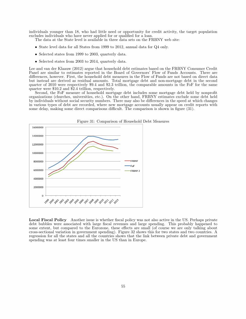
individuals younger than 18, who had little need or opportunity for credit activity, the target populationexcludes individuals who have never applied for or qualified for a loan.

The data at the State level is available in three data sets on the FRBNY web site:

• State level data for all States from 1999 to 2012, annual data for Q4 only.

• Selected states from 1999 to 2003, quarterly data.

• Selected states from 2003 to 2014, quarterly data.

Lee and van der Klaauw (2012) argue that household debt estimates based on the FRBNY Consumer CreditPanel are similar to estimates reported in the Board of Governors’ Flow of Funds Accounts. There aredifferences, however. First, the household debt measures in the Flow of Funds are not based on direct databut instead are derived as residual amounts. Total mortgage debt and non-mortgage debt in the secondquarter of 2010 were respectively $9.4 and $2.3 trillion, the comparable amounts in the FoF for the samequarter were $10.2 and $2.4 trillion, respectively.

Second, the FoF measure of household mortgage debt includes some mortgage debt held by nonprofitorganizations (churches, universities, etc.). On the other hand, FRBNY estimates exclude some debt heldby individuals without social security numbers. There may also be differences in the speed at which changesin various types of debt are recorded, where new mortgage accounts usually appear on credit reports withsome delay, making some direct comparisons difficult. The comparison is shown in figure (31).

Figure 31: Comparison of Household Debt Measures

Local Fiscal Policy Another issue is whether fiscal policy was not also active in the US. Perhaps privatedebt bubbles were associated with large fiscal revenues and large spending. This probably happened tosome extent, but compared to the Eurozone, these effects are small (of course we are only talking aboutcross-sectional variation in government spending). Figure 32 shows this for two states and two countries. Aregression for all the states and all the countries shows that the link between private debt and governmentspending was at least four times smaller in the US than in Europe.

55

Figure 32: Government Spending

.2.2

5.3

.35

.4.4

5

2000 2004 2008 2012year

Spain Ireland Florida Arizona

Government Spending

We therefore argue that the US provides a benchmark for private deleveraging without sudden stops,and with relatively neutral (cross-sectional) fiscal policy.

B.2 Scaled dataThe scaled data for the reduced form shocks for household and public debt, government expenditures andtransfers, spreads and foreign demand are given in figures (33), (34), (36) and (35).

Figure 33: Household and public debt

0.5

11.5

20

.51

1.5

20

.51

1.5

2

2000 2004 2008 2012

2000 2004 2008 2012 2000 2004 2008 2012 2000 2004 2008 2012

AUT BEL DEU ESP

FIN FRA GRE IRL

ITA NLD PRT

Scaled household debt Scaled public debt

year

Graphs by country

56

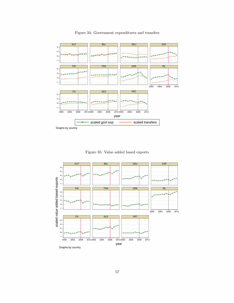
Figure 34: Government expenditures and transfers

.1.2

.3.4

.1.2

.3.4

.1.2

.3.4

2000 2004 2008 2012

2000 2004 2008 2012 2000 2004 2008 2012 2000 2004 2008 2012

AUT BEL DEU ESP

FIN FRA GRE IRL

ITA NLD PRT

scaled govt exp scaled transfers

year

Graphs by country

Figure 35: Value added based exports

.1.2

.3.4

.5.1

.2.3

.4.5

.1.2

.3.4

.5

2000 2004 2008 2012

2000 2004 2008 2012 2000 2004 2008 2012 2000 2004 2008 2012

AUT BEL DEU ESP

FIN FRA GRE IRL

ITA NLD PRT

scale

d v

alu

e a

dded b

ased e

xport

s

yearGraphs by country

57

Figure 36: Spreads (10 year government bonds)

0.0

5.1

.15

.20

.05

.1.1

5.2

0.0

5.1

.15

.2

2000 2004 2008 2012

2000 2004 2008 2012 2000 2004 2008 2012 2000 2004 2008 2012

AUT BEL DEU ESP

FIN FRA GRE IRL

ITA NLD PRT

rho Spread (%)

year

Graphs by country

B.3 Simulation of the reduced form and structural modelsTo run the simulations, we first need to set the initial conditions in a particular year. We use 2002 as ourbase year.

1. Natural employment and prices (unit labor costs) are normalized to n? = 1 and phj,t0 = 1 (so nominalGDP is normalized in the base year to: yj,t0 = 1)

2. Variables set to their observed values are: bhj,t0 , zj,t0 , gj,t0 , bgj,t0

, bgj,t0−1, rj,t0 . We then get fj,t0 , τj andyj,t0 from market clearing and budget constraints:

(a) Foreign demand fj,t0 is chosen to match net exports ej,t0 = 1αj

(fj,t0 − (1− αj) (yj,t0 − gj,t0))

(b) Get τj from the government budget constraint gj,t0 + zj,t0 − τjyj,t0 =bgj,t0+1

1+rj,t0− bgj,t0

(c) Disposable income at time t0 is yj,t0 = (1− τj) yj,t0 + zj,t0

3. Savers’ assets sj,t0 and sj,t0−1 are chosen to solve the equilibrium conditions

(a) sj,t = (1 + ρj,t) (sj,t−1 + yj,t)− Et [yj,t+1]

(b) (1− αj)Et [yj,t+1] = r1+r

(αj (1− χj) sj,t+1 − αjχjbhj,t+1 − b

gj,t+1

)+ fj,t.

(c) (1− αj) yj,t = αjχj

(bhj,t+1

1+rj,t− bhj,t

)+ αj (1− χj)

(sj,t − sj,t+1

1+rj,t

)+

bgj,t+1

1+rj,t− bgj,t + fj,t.

We then feed exogenous processes for the different shocks (using scales values) for observed household debt(bhj,t), fiscal policy (τj , zj,t,gj,t), and interest rate spreads ρj,t. For the sake of completeness, we also feedexogenous foreign nominal demand shocks fj,t, even though they are not crucial for our analysis. For each

58

country, we simulate the path between 2001 and 2012 of nominal GDP yj,t, employment nj,t, wages wj,t, netexports ej,t and public debt bgj,t.

The level of output, the price level and the level of net foreign assets is set to their 2002 levels in thedata. Foreign demand is set using data on exports in value added terms for 2001-2012, normalized so thatthe level of foreign demand in 2002 satisfies goods market clearing in the model. Finally, taxes are set sothat the path for government debt implied by the model coincides with the data.17

The structural model is simulated in the same way but the exogenous variables are replaced by structuralequations (16) and (17) for private debt and spreads respectively and the fiscal policy rule (18). The tax rateis constant at its 2002 level and equal to total government revenues as a percentage of GDP. The structuralshocks are now bhj,t, σt and gj,t.

B.4 Fiscal DevaluationWe define a fiscal devaluation as the combination of a VAT tax on domestic expenditures (private andpublic) and a payroll subsidy. Let phj,t be the price of home goods for domestic consumers, and p∗j,tbe the price of home goods for foreign consumers. τv,j,t is the VAT so that the government collectsτv,j,t (χjxb,j,t + (1− χj)xs,j,t + gj,t). The VAT is paid by firms and rebated to exporters. λj,t is the payrollsubsidy so the government pays λj,twj,tnj,t to firms. Profit maximization implies the following prices:

(1− τv,j,t) phj,t = p∗j,t = (1− λj,t)wj,t

So foreign demand becomes fj,t(1−τv,j,t)phj,t

. Given that the VAT is imposed on imported goods, importers

(assuming flexible prices for foreign firms as for domestic firms) increase the price of their imports to compen-sate for the VAT, so we have pfj,t =

pft1−τv,j,t

where pfj,t is the domestic price of foreign goods in countryj and

pft is the foreign price of foreign goods. With log preferences, this leads to a one for one drop in the quantityof imported foreign goods, while the spending shares remain the same. For simplicity we further assumethat the VAT rate and payroll subsidies are equal, τv,j,t = λj,t so that phj,t = wj,t, yj,t = wj,tnj,t = pj,tnj,tand domestic prices to domestic consumers are unchanged. The government budget constraint, is then:

bgj,t+1

1 + rj,t+ (τj,t − τv,j,t)wj,tnj,t + τv,j,t(χjxb,j,t + (1− χj)xs,j,t + gj,t) = gj,t + zj,t + Γj,t + bgj,t,

where Γj,t is a lump sum transfer to households. We set this transfer so that the fiscal devaluation isneutral for the government budget constraint in the sense that the budget constraint remains:

bgj,t+1

1 + rj,t+ τj,tyj,t = gj,t + zj,t + bgj,t,

so the lump sum transfer is:

Γj,t = τv,j,t(χjxb,j,t + (1− χj)xs,j,t + gj,t)− τv,j,twj,tnj,t17Instead of using government debt directly from data, we construct a simulated government debt series in order to avoid

including factors that affect government debt in the data but are not in the model, such as bank recapitalizations, default, rev-enues from privatizations, etc. The simulated debt series is constructed by adding to t−1 period debt government expendituresincluding interest payments and subtracting tax revenues.

59

Market clearing becomes:

nj,t = αjχjxb,j,t + (1− χj)xs,j,t

phj,t+

fj,t(1− τv,j,t)phj,t

+gj,tphj,t

,

and budget constraints are

xb,j,t =bhj,t+1

1 + rj,t+ yj,t − bhj,t

and

xs,j,t = sj,t + yj,t −sj,t+1

1 + rj,t

where net income is now defined as :

yj,t = (1− τj) yj,t + zj,t + Γj,t

If we substitute the government budget constraint into market clearing, we get:yj,t =

(αj +

τv,j,t

1−τv,j,t

)(χjxb,j,t + (1− χj)xs,j,t)+ fj,t

1−τv,j,t+ 1

1−τv,j,t

(bgj,t+1

1+rj,t− bgj,t − zj,t − Γj,t

)+

(τj−τv,j,t)1−τv,j,t

yj,t

Substitute for consumptions from the budget constraints to get:

(1− αj) yj,t =(αj +

τv,j,t

1−τv,j,t

)[χj

(bhj,t+1

1+rj,t− bhj,t

)+ (1− χj)

(sj,t − sj,t+1

1+rj,t

)]+ 1

1−τv,j,t

(fj,t +

bgj,t+1

1+rj,t− bgj,t

)Assuming permanent taxes and subsidies, permanent shocks on foreign demand, iid spreads and Et

[bgj,t+2

]=

bgj,t+1, expected market clearing at t+ 1 is:

(1− αj)Et [yj,t+1] = r1+r

((αj +

τv,j,t

1−τv,j,t

) ((1− χj) sj,t+1 − χjbhj,t+1

)− 1

1−τv,j,tbgj,t+1

)+

fj,t1−τv,j,t

So the equilibrium equations in the case of a fiscal devaluation (with VAT and payroll subsidy equal toτv,j,t) and revenue neutrality become:

1. sj,t+1 = (1 + ρj,t) (sj,t + yj,t)− Et [yj,t+1]

2. (1− αj)Et [yj,t+1] = r1+r

((αj +

τv,j,t

1−τv,j,t

) ((1− χj) sj,t+1 − χjbhj,t+1

)− 1

1−τv,j,tbgj,t+1

)+

fj,t1−τv,j,t

3. (1− αj) yj,t =(αj +

τv,j,t

1−τv,j,t

)[χj

(bhj,t+1

1+rj,t− bhj,t

)+ (1− χj)

(sj,t − sj,t+1

1+rj,t

)]+ 1

1−τv,j,t

(fj,t +

bgj,t+1

1+rj,t− bgj,t

)4.

bgj,t+1

1+rj,t− bgj,t = (1− τv,j,t) (gj,t + zj,t − τjyj,t)

5. yj,t = (1− τj) yj,t + zj,t + Γj,t

6. Γj,t = τv,j,t

[1−αj

αj(yj,t − gj,t) + 1

αj

fj,t1−τv,j,t

]

60