Embed Size (px)
Citation preview

InsightVideo: Towards hierarchical video content organization for
efficient browsing, summarization and retrieval
Xingquan Zhua, Ahmed K. Elmagarmida, Xiangyang Xueb, Lide Wub, Ann Christine Catlina
aDept. of Computer Science, Purdue University, West Lafayette, IN 47907, USA
{zhuxq, ake, acc}@cs.purdue.edu bDept. of Computer Science, Fudan University, Shanghai 200433, P.R. China
{xyxue, ldwu}@fudan.edu.cn
ABSTRACT
Hierarchical video browsing and feature-based video retrieval are two standard methods for accessing video content. Very little research, however, has addressed the benefits of integrating these two methods for more effective and efficient video content access.
In this paper we introduce InsightVideo, a video analysis and retrieval system, which joins video content hierarchy, hierarchical browsing and retrieval for efficient video access. We propose several video processing techniques to organize the content hierarchy of the video. We first apply a camera motion classification and key-frame extraction strategy that operates in the compressed domain to extract video features. Then, shot grouping, scene detection and pairwise scene clustering strategies are applied to construct the video content hierarchy. We introduce a video similarity evaluation scheme at different levels (key-frame, shot, group, scene, and video.) By integrating the video content hierarchy and the video similarity evaluation scheme, hierarchical video browsing and retrieval are seamlessly integrated for more efficient video content access. We construct a progressive video retrieval scheme to refine user queries through the interaction of browsing and retrieval. Experimental results and comparisons of camera motion classification, key-frame extraction, scene detection, and video retrieval are presented to validate the effectiveness and efficiency of the proposed algorithms and the performance of the system. Keywords: Hierarchical video content organization, video browsing, video retrieval, camera motion classification, key-frame extraction, scene detection, video similarity assessment.
1. INTRODUCTION
Recent advances in high-performance networking and improvements in computer hardware have led to the
emergence and proliferation of video and image-based applications. Database management techniques for
traditional textual and numeric data cannot handle video data; therefore, new models for storage and retrieval
must be developed. In general, a video database management system should address two different problems:
(1) the presentation of video content for browsing, and (2) the retrieval of video content based on user
queries.
Some methods have been developed for presenting video content by hierarchical video shot clustering
[1][2], organizing video storyboards [3] or joining spatial-temporal content analysis and progressive retrieval
for video browsing [4]. These methods allow a viewer to rapidly browse through a video sequence, navigate
from one segment to another, and then either get a quick overview of video content or zoom to different
levels of detail to locate segments of interest. These systems may be efficient in video browsing and content

presentation, however they fail either in detecting semantically related units for browsing [1,2,4] or in
integrating efficient video retrieval with video browsing [3].
Compared with video content presentation, more extensive research has been done in the area of video
retrieval. Several research and commercial systems have been developed which provide automatic indexing,
query and retrieval based on visual features, such as color and texture [5-12], and others execute queries on
textual annotation [13]. Elmagarmid, et al. [14] has published a comprehensive overview of this topic.
The first video parsing, indexing and retrieval framework was presented by Zhang, et al. [2], it uses the
annotations and visual features of key-frames for video browsing and retrieval. QBIC [12] supports shape
queries for semi-manually extracted objects. The Virage [8] system supports feature layout queries, and users
can assign different weights to different features. The Photobook system [9] enables users to plug in their
own content analysis procedures. Cypress [11] allows users to define concepts using visual features like
color. VisualSEEk [10] allows localized feature queries and histogram refinements for feedback using a web-
based tool. Systems such as CVEPS [15] and JACOB [16] support automatic video segmentation and video
indexing based on key-frames or objects. The web-based retrieval system, WebSEEK [17], builds several
indexes for images and video based on visual features and non-visual features. The Informedia digital video
library project [18] has done extensive research in mining video knowledge by integrating visual features,
closed caption, speech recognition etc. A more advanced content-based system, VideoQ [7], supports video
query by single or multiple objects, using many visual features such as color, texture, shape and motion.
However, the video retrieval approaches introduced above usually just add the functionalities for shot
segmentation and key-frames extraction to existing image retrieval systems. After shot detection and key-
frame extraction, they merely apply similarity measurements based on low-level features of the video frames
or shots. This is not satisfactory because video is a temporal media, the sequencing of individual frames
creates new semantics that may not be present in any of the individually retrieved shots.
A naïve user is interested in querying at the semantic level, rather than having to use features to describe
his (her) concept. In most cases it is difficult to express concepts using feature matching, and even a good
match in terms of feature metrics may yield poor query results for the user. For example, in multiple domain
recall, a query for 60% green and 40% blue may return an image of a grass and sky, a green board on a blue
wall or a blue car parked in front of a park, as well as many others. Helping users to find query examples and
refine their queries is also an import feature for video retrieval systems. However, instead of integrating the
efficient video browsing and retrieval together, the systems described above emphasize either browsing or
retrieval. A progressive strategy should be developed to join the video browsing and retrieval schemes
together to improve the effectiveness and efficiency of both.
Based on these observations, we propose a novel video content organization and accessing model for
video browsing and retrieval. A progressive video retrieval scheme is formed by executing the browsing and
retrieval iteratively. The distinct features of our system are the following: (1) several novel video processing
techniques are introduced which improve existing algorithms in important areas, (2) a video content
hierarchy is constructed which allows hierarchical video browsing and summarization to be executed directly

and efficiently, (3) by addressing video similarity at different levels and granularity, our retrieved results
mostly consist of visually and semantically related units, and (4) the seamless integration of video browsing
and retrieval allows users to efficiently shrink and refine their queries.
Hierarchical video content organization
Hierarchical video content table
Video browsing Video retrieval
Video content database, video feature database
Query Refine Users
Video Shot segmentation Camera motion classification
Key-frame extraction
Shot grouping Scene detection Scene clustering
Video feature extraction
Video analysis and feature extraction
Progressive video content access
Figure 1. System flow for InsightVideo
2. THE SYSTEM OVERVIEW
The process flow for the InsightVideo system is illustrated in Figure 1. The system consists of three parts:(1)
video analysis and feature extraction, (2) hierarchical video content organization, and (3) progressive video
content access. To extract video features, a shot segmentation algorithm is applied to each input video. Then,
for each segmented shot, the camera motion classification strategy is utilized to qualitatively classify camera
motions. Based on identified motion information, key-frame extraction is executed to select the key-frame(s)
for each shot. The detected camera motions and low-level features are utilized for video similarity evaluation.
After the video features have been extracted, the video content table is constructed by shot grouping, scene
detection, and scene clustering strategies to generate a three layer video content hierarchy (group, scene,
clustered scene).
Based on this video content hierarchy and extracted video features, we propose a progressive video
content access scheme in which we first address the video similarity evaluation scheme at different levels and
then integrate the hierarchical video browsing and retrieval for video content access and progressive retrieval.
Using hierarchical video browsing, a user is provided with an overview of video content from which a query
example can be selected. Then, video retrieval is invoked to produce a list of similar units, and the user can
browse the content hierarchy of retrieved results to refine the query. By iteratively executing the retrieval and
browsing, a user’s query can be quickly refined to retrieve the unit of interest.
The remainder of this paper is organized as follows. Section 3 presents several video analysis and feature
extraction techniques, including camera motion classification and key-frame extraction schemes. Then, based
on extracted video features, Section 4 introduces techniques for hierarchical video content organization. In
Section 5, the video similarity assessment scheme is applied at different levels of the video content hierarchy.
Section 6 presents techniques that joint hierarchical video browsing and retrieval for efficient video content
access. The conclusion and remarks are given in Section 7.

3. VIDEO ANALYSIS AND FEATURE EXTRACTION
Most schemes for video feature extraction begin by segmenting contiguous frames into separate shots, and
then selecting key-frames to represent shot content. With this scheme, a video database is treated somewhat
like an image database, because the motion information in the video (or shot) is missed. In our system, the
motion information in the video is detected and extracted as a shot feature to help in identifying video
content. We first apply shot segmentation to the video. Then the camera motion classification scheme is
executed. Based on extracted motion information, a key-frame extraction scheme is proposed and the camera
motion in the shot will also be utilized as the features to evaluate similarity between shots.
A great deal of research has been done in shot boundary detection, and many approaches achieve
satisfactory performance [1][19]. In previous work, we have developed a shot segmentation approach with an
adaptive threshold selection for break and gradual shot detection [20]. In the next sections, we will introduce
the camera motion classification and key-frame extraction schemes.
3.1 Camera Motion Classification
Motion characterization plays an important role in content-based video indexing. It is an essential step in
creating compact video representation automatically. For example, a mosaic image can represent a panning
sequence [21]; the frames before and after a zoom can represent the zoom sequence. As the research work in
[53] has demonstrated, in addition to various visual features, the motion information in video shots can also
be explored for content-based video retrieval. Thus, an effective characterization of camera motion greatly
facilitates the video representation, indexing and retrieval tasks. And the proposed multimedia content
description standard MPEG-7 [59] has also adopted various descriptors (DS) to qualitatively (different types
of motions) and quantitatively (the amount of motions) describe the camera motion in each shot [57-58].
To extract the camera motion, Ngo et al. [22] proposed a method using temporal slice analysis for
motion characterization, however, to distinguish different motion patterns in the slice is a challenging task for
videos with cluttered background or containing moving objects. Srinivasan et al. [24] introduced a qualitative
camera motion extraction method that separates the optical flow into two parts, parallel and rotation, for
motion characterization. Xiong et al. [23] presented a method that analyzed spatial optical flow distribution.
However, these last two methods can only be used when the Focus of Expansion (FOE) or Focus of
Contraction (FOC) [25] is at the center of the image, and this is not always the case in generic videos.
To analyze camera motion in the compressed domain, Tan et al. [26], Kobla et al. [27] and Dorai et al.
[28] presented three methods based on motion vectors in MPEG streams. In [26], a 6-parameters
transformation model is utilized to classify camera motions into panning, tilting and zooming. The methods
in [27][28] map motion vectors in current frame into eight directions. Motion classification was developed
based on the values in these eight directions. However, these strategies are sensitive to noise in motion
vectors and fail to detect the camera rolling. Furthermore, extracted optical flow or motion vectors may
contain considerable noise or error, which significantly reduces the efficiency of their strategies.

We have found that the statistical information for the mutual relationship between any two motion
vectors is relatively robust to noise (see Figure 3.) For a given type of camera motion contained in the current
frame, the statistical mutual relationship in the frame will show a distinct distribution tendency. Based on this
observation, we propose a qualitative camera motion classification method. In addition to detecting most
common camera motions (pan, tilt, zoom, still), our method can also detect camera rolling, and various
detected camera motions will directly comply with the motion descriptors in MPEG-7 standard [59].
3.1.1 Problem Formulation
Our objective is to efficiently process videos stored in MPEG format for camera motion classification. As
shown in Figure 2, the syntax of MPEG-1 video defines four types of coded pictures: intracoded pictures (I-
frames), predicted pictures (P-frames), bidirectionally predicted pictures (B-frames), and DC encoded frames
(which are now rarely used). These pictures are organized into sequences of groups of pictures (GOP). Each
video frame is divided into a sequence of nonoverlapping macroblocks (MB), such that each MB is then
either intracoded or intercoded. An I-frame is completely intracoded, and the MB in P-frame may be
separated into two types: intracoded (containing forward prediction motion vectors) and intercoded
(containing no motion vectors). In this paper, we use only the motion vectors from P-frames, that is, we are
sampling the camera motion. For example, if the MPEG video is coded at a rate of 30 frames per second
using the GOP in Figure 2, there are 8 P-frames per second in the video. We will require the underlying
camera motion rates (per frame) to have a bandwidth of less than 4 Hz. For most videos, this is a reasonable
assumption. Using the motion vectors from both the P and B-frames has the potential to yield better
accuracy, but at the cost of increased computation. In our classification scheme, we assume that there is no
large object motion or the motion caused by large objects can be ignored. Thus, only the dominant camera
motion is detected.
3.1.2 The mutual relationship between motion vectors
Given two points A, B in current frame Pi with positions pA=(xA, yA), pB= (xB, yB) and motion vectors
VA=(uA,vA) and VB=(uB,vB), we denote the vector from point A to B as ABV�
, and the line cross point A and B
as BA
BABA
BA
BA
xxxyyxx
xxyyy
−+
−−= − . As shown in Figure 3, there are four types of mutual relationships between
VA and VB: approach, parallel, diverging and rotation.
To classify the mutual relationship between VA and VB, we first measure whether they are on the same
side (Figure 3(A)) or different sides (Figure 3(B)) of vector ABV�
. Based on the geometry relationship among
the four points (xA, yA), (xA+uA, yA+vA), (xB, yB) and (xB+uB, yB+vB), it is obvious that if VA and VB are on the
same side of vector ABV�
, both points (xA+uA, yA+vA) and (xB+uB, yB+vB) should be above or below the line
which crosses point A and B at the same time. Hence, we multiple y1 and y2 (from Eq. (1)).. If the product is

non-negative, we will claim VA and VB are on the same side of vector ABV�
; otherwise, AV and BV are on
different sides of vector ABV�
.
−−+⋅
−−−+=
−−+⋅
−−−+=
−
−
BA
BABAAA
BA
BAAA
BA
BABAAA
BA
BAAA
xxxyyxux
xxyyvyy
xxxyyxux
xxyyvyy
)(
)(
2
1 (1)
As shown in Figure 3, if we assume that α denotes the angle between ABV�
and VA, and β denotes the angle
between VB and ABV�
, if VA and VB are on the same side of ABV�
, then their mutual relationship is classified as
follows:
• If α+β < 180° - TPARA, the mutual relationship between VA and VB is approach.
• If α+β > 180° + TPARA, the mutual relationship between VA and VB is diverging.
• Otherwise, the mutual relationship between VA and VB is parallel.
If VA and VB are on different sides of ABV�
, then their mutual relationship is classified as follows:
• If α+β < TCLOSE, the mutual relationship between VA and VB is approach.
• If α+β > TFAR, the mutual relationship between VA and VB is diverging.
• Otherwise, the mutual relationship between VA and VB is rotation.
In our system, we set TPARA, TCLOSE and TFAR to 15°, 60° and 250° respectively.
3.1.3 The relationship between camera motion and motion vectors
Figure 4 shows the relationship between the camera motion and motion vectors contained in the frame:
• If the camera pans or tilts, most motion vectors’ mutual relationships in the frame are parallel.
• If the motion of the current frame is zooming, most motion vectors’ mutual relationships in current
frame either approach to (zoom out) FOC or diverge from (zoom in) FOE.
• If the camera rolls, most vertical vectors’ (defined in Section 3.1.4.4) mutual relationship in the
frame either approach to (Roll_Clockwise) FOC or diverge from (Roll_AntiClockwise) FOE.
Based on these observations, a motion feature vector is constructed to characterize the motion vectors.
I P P B B B B P PB B B B B B
F o rw a rd p re d ic tio n
B id ir e c t io n a l p re d ic tio nB id i re c tio n a l p r ed ic t io n
G ro u p o f P ic tu re (G O P )
A B
A B
A B
(a) approach (b) parallel (c) diverging
(A) The mutual relationship between motion vectors on the same side of vector ABV�
A B
AB
A
B
(a) approach (b) diverging (c) rotation
(B) The mutual relationship between motion vectors on different side of vector ABV�
α β α α β β
α
α α
β β β
VA VA VA
VA VA VA
VB VB VB
VB
VB VB
Figure 2. GOP structure Figure 3. Mutual relationship between motion vectors

0
0.2
0.4
0.6
0.8
1
1 2 3 4 5 6 7 8 9 10 11 12 13 14
14 bins motion featurevector
Valu
e
Tilt up
Tilt up
0
0.2
0.4
0.6
0.8
1
1 2 3 4 5 6 7 8 9 10 11 12 13 14
14 bins motion feature vector
Val
ue
Pan right
Pan right
0
0.2
0.4
0.6
0.8
1
1 2 3 4 5 6 7 8 9 10 11 12 13 14
14 bins motion feature vector
Valu
e
Zoom in
Zoom in
0
0.2
0.4
0.6
0.8
1
1 2 3 4 5 6 7 8 9 10 11 12 13 14
14 bins motion feature vector
Valu
e
Zoom out
Zoom out
0
0.2
0.4
0.6
0.8
1
1 2 3 4 5 6 7 8 9 10 11 12 13 1414 bins motion feature vector
Val
ue
Roll_AntiClockwise
Roll_AntiClockwise (a) (b) (c) (d) (e)
Figure 4. The relationship between camera motion and motion vectors. The column (a), (b), (c), (d) and (e)
indicate the current P-frame (Pi), motion vectors in Pi, the succeeding P-frame (Pi+1), motion vectors in Pi+1,
and the 14-bin motion feature vector distribution for (d) respectively. The black block in motion vectors
indicate the “intracoded macroblock”; hence, no motion vector is available for those blocks.
3.1.4 Motion feature vector construction
In this subsection, we introduce four histograms to characterize motion vectors in each frame. A 14-bin
feature vector is then formed by packing these four histograms sequentially from bin 1 to bin 14.
3.1.4.1 Motion vector energy histogram (Hme)
For any P-frame Pi and its motion vectors, we assume there are N MB contained in Pi. We denote APi as the
aggregation of all available motion vectors (intercoded MB) in Pi, and the number of motion vectors in APi is
denoted by Nmv. Given point A (PA=(xA,yA)) in Pi and its motion vector VA=(uA,vA), then Eq. (2) defines the
energy of VA.
222AAA vuV += (2)

Assuming SPi denotes the aggregation of motion vectors in APi with energy smaller than a given threshold
TSMALL, the number of vectors in SPi is denoted by Nsmall. We calculate the mean µ and variance δ of the
motion vectors in SPi. If we assume LPi denotes the aggregation of motion vectors in APi whose distance to µ
is larger than TLOC, and the number of vectors in LPi is denoted by Nloc. The motion vector energy histogram
(Hme) is constructed using Eq. (3).
N
NHNNNNH small
melocmv
me =+−= ]1[;)(]0[ (3)
In our system, we set TLOC=1.5δ and TSMALL=2 respectively. In the next section, the motion vectors in
aggregation VPi, VPi= )( iii LPSPAP ∪∩ , is referred to as the valid motion vectors in Pi, i.e., the valid motion
vectors are those with relatively high energy and low variance.
3.1.4.2 Motion vector orientation histogram (Hmo)
Clearly, the orientations of the valid motion vectors VPi in Pi will help us determine the direction of the
camera motion. For each motion vector ),( AAA vuV = in VPi, we denote D(VA) as its orientation, and then divide
all valid motion vectors’ orientations into four categories: (-45°, 45°), (45°, 135°), (135°, 225°), (225°, 315°).
The motion vector orientation histogram is constructed using Eq. (4).
3,2,1,0;1
)( 9045)(9045,; =−
=∑
⋅+≤<⋅+−∈ kNN
kHsmallmv
kVDkVPVVmo
AiAA���� (4)
3.1.4.3 Motion vector mutual relationship histogram (Hmr)
Given two motion vectors in VPi, their mutual relationship is classified with the strategy given in Section
3.1.2. The histogram of the mutual relationships in Pi are then calculated and put into different bins of
histogram Hmr, with Hmr[0], Hmr[1], Hmr[2] and Hmr[3] corresponding to approach, diverging, rotation and
parallel, respectively.
3.1.4.4 Motion vector vertical mutual relationship histogram (Hmvr)
As described in Section 3.1.3, if the camera rolls, the mutual relationships of most motion vectors’ vertical
lines will approach to FOC or diverge from FOE. Hence, given any motion vector VA=(uA,vA) in VPi, its
vertical vector is defined by ),( AAA uvV −=′ , and we can use the strategy in Section 3.1.2 to calculate the
mutual relationship for any two vertical vectors AV ′ and BV ′ in VPi. The histogram constructed in this way is
denoted as the vertical mutual relationship histogram (Hmvr) with Hmvr[0], Hmvr[1], Hmvr[2] and Hmvr[3]
representing approach, diverging, rotation and parallel, respectively.
3.1.5 Camera motion classification
The experimental results in Figure 4 (e) show that for any type of camera motion, the 14-bin motion feature
vector will have a distinct distribution mode. For example, when the camera pans, Hmr[3] will contain the
largest value in Hmr, and the bin with the largest value in Hmo will indicate the direction of the panning. For

zooming operations, either Hmr[0] or Hmr[1] will have the largest value in Hmr. If the camera rolls, Hmr[2]
will have the largest value in Hmr, and either Hmvr[0] or Hmvr[1] have the largest value in Hmvr. Hence, based
on the 14-bin vector, a qualitative camera motion classification strategy is presented:
Input: 14-bin motion feature vector of current P-frame Pi.
Output: The motion category (pan left, pan right, tilt up, tilt down, zoom in, zoom out, roll_clockwise,
roll_anticlockwise, still, unknown) Pi belongs to, denoted as “Pi ← ? ”.
Procedure:
1. If Hme[0] is larger than threshold TUNK, Pi ← “unknown”, otherwise go to step 2.
2. If Hme[1] is larger than threshold TSTILL, Pi ← “still”, if not go to step 3.
3. If Hme[0]+Hme[1] is larger than threshold TUNION, Pi ← “unknown”, otherwise, go to step 4.
4. Find the largest and second largest values among Hmr and denote them as maxmrH and sec
mrH respectively.
If the ratio between secmrH and max
mrH is larger than threshold TREL, Pi ← “unknown”, otherwise, the
steps below is used for classification.
• If maxmrH = Hmr[0], then Pi ← “zoom out”; else if max
mrH = Hmr[1], Pi ← “zoom in”.
• If maxmrH =Hmr[2], go to step 6; else if max
mrH = Hmr[3], go to step 5.
5. Find the maximal value among Hmo and denote it as maxmoH :
• If maxmoH = Hmo[0], Pi ← “panning left”; else if max
moH equals Hmo[1], Pi ← “tilting down”.
• If maxmoH = Hmo[2], Pi ← “panning right”; else if max
moH equals Hmo[3], Pi ← “tilting up”.
6. Find the maximal value among Hmvr and denote it as maxmvrH :
• If maxmvrH =Hmvr[0], Pi ← “roll_anticlockwise”; else If max
mvrH = Hmvr[1], Pi ←
“roll_clockwise”; Otherwise, Pi ← “unknown”.
The thresholds TUNK, TSTILL, TREL and TUNION may be determined by experiments; in our system we set
them to 0.55, 0.5, 0.8 and 0.8, respectively.
There is little doubt that some conditions could exist which might result in an incorrect classification of
the camera motion. Since the camera motion should be consistent over a certain length of time, the temporal
filter operation is used to eliminate those errors, that is, any camera motion lasting less than 3 P-frames is
absorbed by preceding or succeeding camera motions. The filtered camera motion information is then stored
as the motion feature of the shot.
3.2 KEY-FRAME EXTRACTION
Key-frame(s) summarize the content of a video shot. Other research has addressed the problem of key-frame
extraction [30-35], and the recent survey can be found in [29] and [55]. A first attempt in key-frame
extraction was to choose the frame appearing at the beginning of each shot as the key-frame [35]. However,

if the shot is dynamic, this strategy will not provide good results. In order to address this problem, clustering
techniques [31] and low-level features [30] are utilized for key-frame extraction by clustering all frames in
the shot into M clusters or calculating accumulated frame differences. Due to the fact that the motions in
video shots imply the content evolution and change, a motion activity-based key-frame extraction method has
been proposed in [54-55], where the MPEG-7 motion intensity in each shot is used to guide the key-frame
selection. Given a user specified number, the system selects the corresponding number of key-frames by
using the cumulative motion intensity, where more key-frames are extracted from the high motion frame
regions. However, determining the number of key-frames that optimally addresses the video content change
is a difficulty. On the other hand, if there is large camera or object motion in the shot, the selected key-frames
may be blurred, and thus not suitable for the key-frame.
The authors in [34] and [32] avoid these problems by proposing threshold-free methods for extracting
key-frames. In [34], the temporal behavior of a suitable feature vector is followed along a sequence of
frames, and a key-frame is extracted at each place of the curve where the magnitude of its second derivative
reaches the local maximum. A similar approach is presented in [32], where the local minima of motion is
utilized for key-frame extraction. However, two problems remain: (1) locating the best range to find the local
minimum is also determined by a critical threshold, and (2) since the small motion of the video can cause the
optical flow have large variations, these methods may address more details when compared with generating
shot content overview.
To extract key-frames using these strategies, the video must be fully decoded. In the next section, we
introduce a threshold-free method that extracts key-frames in the compressed domain. Our method is based
on the method from literature [32], however, there are several distinguishing elements: (1) our method is
executed in the compressed domain (only a very limited number of frames need to be decoded), (2) instead of
using optical flow, we use motion vectors from the MPEG video, and (3) instead of using the threshold, we
use camera motions in the shot to determine the local maximum or minimum.
3.2.1 The Algorithm
Our key-frame extraction algorithm is executed using the following steps:
1. Given any shot Si, use the camera motion classification and temporal motion filter to detect and
classify the camera motions, as shown in Figure 5.
2. Find the representative frame(s) for each type of motion (see Figure 5), and the collection of all
representative frames is taken as the key-frames for Si.
From the start frame to the end frame in shot Si, for any given P-frames (Pi) we denote APi as the
aggregation of all available motion vectors in Pi. Then Eq. (5) is used to calculate the motion magnitude of Pi
iiikkkkk PAPAPVvuVVkki vuPM
⊂∈=∑ +=
,),,(,
22 )()( (5)
where Vk denotes the motion vectors in Pi. Given Pi, its M(Pi) is influenced by two factors:
• The motion information contained in Pi. The smaller the amount of motion, the smaller M(Pi) is.
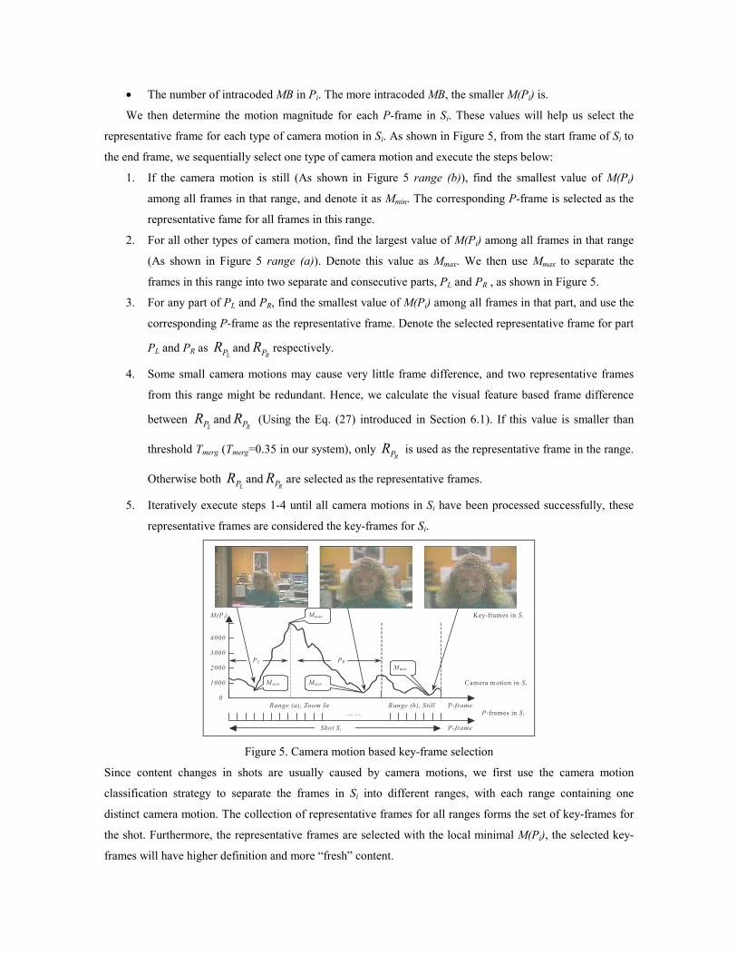
• The number of intracoded MB in Pi. The more intracoded MB, the smaller M(Pi) is.
We then determine the motion magnitude for each P-frame in Si. These values will help us select the
representative frame for each type of camera motion in Si. As shown in Figure 5, from the start frame of Si to
the end frame, we sequentially select one type of camera motion and execute the steps below:
1. If the camera motion is still (As shown in Figure 5 range (b)), find the smallest value of M(Pi)
among all frames in that range, and denote it as Mmin. The corresponding P-frame is selected as the
representative fame for all frames in this range.
2. For all other types of camera motion, find the largest value of M(Pi) among all frames in that range
(As shown in Figure 5 range (a)). Denote this value as Mmax. We then use Mmax to separate the
frames in this range into two separate and consecutive parts, PL and PR , as shown in Figure 5.
3. For any part of PL and PR, find the smallest value of M(Pi) among all frames in that part, and use the
corresponding P-frame as the representative frame. Denote the selected representative frame for part
PL and PR as LPR and
RPR respectively.
4. Some small camera motions may cause very little frame difference, and two representative frames
from this range might be redundant. Hence, we calculate the visual feature based frame difference
between LPR and
RPR (Using the Eq. (27) introduced in Section 6.1). If this value is smaller than
threshold Tmerg (Tmerg=0.35 in our system), only RPR is used as the representative frame in the range.
Otherwise both LPR and
RPR are selected as the representative frames.
5. Iteratively execute steps 1-4 until all camera motions in Si have been processed successfully, these
representative frames are considered the key-frames for Si.
… …
Shot Si
Range (a), Zoom In Range (b), Still
P-frame
P-frame
M min
M min Mmin
Mmax
PL PR
M(Pi)
1000
2000
3000
4000
Camera motion in Si
P -frames in Si
Key-frames in Si
0
Figure 5. Camera motion based key-frame selection
Since content changes in shots are usually caused by camera motions, we first use the camera motion
classification strategy to separate the frames in Si into different ranges, with each range containing one
distinct camera motion. The collection of representative frames for all ranges forms the set of key-frames for
the shot. Furthermore, the representative frames are selected with the local minimal M(Pi), the selected key-
frames will have higher definition and more “fresh” content.

By adopting motion activity in camera motion selection, our method is also similar to the scheme in [54-
55]. However, there are two key distinctions: (1) with the method in [54-55], it’s the authors but not the
system to determine the number of key-frames to be extracted from each shot. Given a video that contains
hundreds of shots, it would be very hard (or even unreasonable) for users to specify the number of key-
frames for each shot. Consequently, the naïve users may simply specify a constant key-frame number for all
shots. In that case, the proposed scheme may introduce redundancy in low motion shots and miss the content
change in high motion shots; (2) the method in [54-55] don’t consider the local motion minimum but use
only the accumulative motion activity, as a result, the select key-frames may be blurred and not clear enough
for the content presentation purpose.
3.3 Experimental Results
3.3.1 Camera motion classification result
Table 1 shows the results produced by our camera motion detection algorithm. We evaluated the efficiency
of our algorithm (denoted by A) through an experimental comparison with transformation model based
method [26]* (denoted by B). Several standard MPEG-I streams (about 11711 frames) were downloaded
from http://www.open-video.org and used as our test bed. One edited MPEG-I file (about 16075 frames)
containing a large number of zooming and roll motions was also used as a test dataset. For better evaluation,
the precision defined in Eq. (6) is used, where nc,nf denote the correctly and falsely detected camera motion
in the P-frames.
Precision=nc / (nc+nf) (6)
Among all 27786 frames in the video, the sequential frame regions with a distinct camera motion (pan,
tilt, zoom, roll, still) are selected as our ground truth. These frames (about 20011 frames) occupy about 72%
of the entire the video, with about 5201 P frames contained in the 20011 frames. Our experiment is executed
with these 5201 P-frames. From Table 1, we find that, on average, our method has a precision of
approximately 80.4%, about 5% higher transformation model based method [26]. In detecting pure panning
and tilting, both methods have about the same precision. However, while some abnormal motion vectors
caused by objects motion or other reasons contained or FOE/FOC is not at the center of the image, the
efficiency of this method is rather reduced, since those motion vectors cannot be characterized by the
proposed transformation model. However, our method is a statistical strategy, the abnormal or distorted
motion vectors would have not much influence in unfolding the dominant camera motion in the frames, thus
resulting in a relatively higher precision. Furthermore, while method B is not able to detect roll motion, our
method produces a precision of 68% for roll detection.
On a PC with PIII 900MHz CUP, the average time to process one P-frame is three times faster than real
time and four times faster than method B.
*Remark: We compare our method with the method in literature [32], since it also works in compressed
domain and utilizes only the motion vector of P-frame for classification.
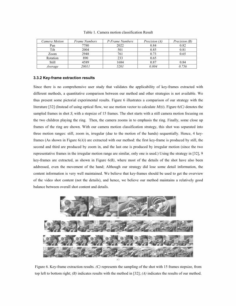
Table 1. Camera motion classification Result
Camera Motion Frame Numbers P-Frame Numbers Precision (A) Precision (B) Pan 7780 2022 0.84 0.82 Tilt 2004 501 0.85 0.81
Zoom 2948 761 0.73 0.65 Rotation 890 233 0.65
Still 4589 1684 0.87 0.84 Average 20011 5201 0.804 0.756
3.3.2 Key-frame extraction results
Since there is no comprehensive user study that validates the applicability of key-frames extracted with
different methods, a quantitative comparison between our method and other strategies is not available. We
thus present some pictorial experimental results. Figure 6 illustrates a comparison of our strategy with the
literature [32] (Instead of using optical flow, we use motion vector to calculate M(t)). Figure 6(C) denotes the
sampled frames in shot Si with a stepsize of 15 frames. The shot starts with a still camera motion focusing on
the two children playing the ring. Then, the camera zooms in to emphasis the ring. Finally, some close up
frames of the ring are shown. With our camera motion classification strategy, this shot was separated into
three motion ranges: still, zoom in, irregular (due to the motion of the hands) sequentially. Hence, 4 key-
frames (As shown in Figure 6(A)) are extracted with our method: the first key-frame is produced by still, the
second and third are produced by zoom in, and the last one is produced by irregular motion (since the two
representative frames in the irregular motion range are similar, only one is used.) Using the strategy in [32], 9
key-frames are extracted, as shown in Figure 6(B), where most of the details of the shot have also been
addressed, even the movement of the hand; Although our strategy did lose some detail information, the
content information is very well maintained. We believe that key-frames should be used to get the overview
of the video shot content (not the details), and hence, we believe our method maintains a relatively good
balance between overall shot content and details.
(A)
(B)
(C) Figure 6. Key-frame extraction results. (C) represents the sampling of the shot with 15 frames stepsize, from
top left to bottom right; (B) indicates results with the method in [32]; (A) indicates the results of our method.

4. HIERARCHICAL VIDEO CONTENT ORGANIZATION
Generally, videos can be represented using a hierarchy of five levels (video, scene, group, shot, and key-
frame)*, increasing in granularity from top to bottom. Much research has addressed the problem of
constructing semantically richer video entities by visual feature based shot grouping [35-38] or joint semantic
rules and knowledge information for scene detection [39-41][50]. However, these strategies only solve the
problem of semantic units detection and visualization. Since similar scenes may appear repeatedly in a video,
redundant scene information should be reduced by clustering beyond the scene level. In this way, a concise
video content table can be created for hierarchical browsing or summarization. Instead of using the semantic
unit for video content table construction, other strategies utilize the video shot (or key-frames) based
clustering strategy [1-2][42] to construct the video content hierarchy. However, the constructed hierarchy just
addresses some low-level feature based frame differences.
To address this problem, we generate a three level hierarchy from clustered scenes to groups. By
integrating video key-frames and shots, a five level video content hierarchy (clustered scene, scene, group,
shot, key-frame) is successfully constructed.
As shown in Figure 1, we construct the video content hierarchy in three steps: (1) group detection, (2)
scene detection, and (3) scene clustering. The video shots are first grouped into semantically richer groups.
Then, similar neighboring groups are merged into scenes. Beyond the scene level, a pairwise cluster scheme
is utilized to eliminate repeated scenes in the video, thus reducing the redundant information. Using the
content structure constructed by this strategy, the hierarchical video browsing and summarization is accessed
directly. In addition, we have also addressed the problem of the representative unit selection for groups,
scenes, and clustered scene units for visualizing the generated video content information.
Generally, the quality of most proposed methods is heavily based on the selection of thresholds [36-38],
however, the content and low-level features among different videos vary greatly. Thus, we use the entropic
threholding technique to select the optimal threshold for video group and scene detection; it has been shown
to be highly efficient for the two-class data classification problem. *Remark: In this paper, the video group and scene are defined as in [37]: (1) A video scene is a
collection of semantically related and temporally adjacent shots, depicting and conveying a high-level
concept or story; (2) A video group is an intermediate entity between the physical shots and semantic scenes;
examples of groups are temporally or spatially related shots.
4.1 Video group detection
The shots in one group usually share similar background or have a high correlation in time series. Therefore,
to segment the spatially or temporally related video shots into groups, a given shot is compared with the shots
that precede and succeed it (no more than 2 shots) to determine the correlation between them, as shown in
Figure 7. Assume StSim(Si, Sj) denotes the similarity between shot Si and Sj, which was given in Eq. (33). Our
group detection procedure is stated as below:

Input: Video shots. Output: Video groups
Procedure:
1. Given any shot Si, if CRi is larger than TH2-0.1:
a. If R(i) is larger than TH1, claim a new group starts at shot Si..
b. Otherwise, go to step 1 to process other shots.
2. Otherwise:
a. If both CRi and CLi are smaller than TH2, claim a new group starts at shot Si.
b. Otherwise, go to step 1 to process other shots.
3. Iteratively execute step 1 and 2 until all shots are parsed successfully.
The definitions of CRi, CLi, R(i) are given in Eq.(7),(8),(9).
CLi =Max{ StSim(Si,Si-1), StSim(Si,Si-2)}; CRi =Max{ StSim(Si,Si+1), StSim(Si,Si+2)} (7)
CLi+1 =Max{ StSim(Si+1,Si-1), StSim(Si+1,Si-2)}; CRi+1 =Max{ StSim(Si+1,Si+2), StSim(Si+1,Si+3)} (8)
R(i)=(CRi+CRi+1)/(CLi+CLi+1). (9)
Since closed caption and speech information is not available in our strategy, the visual features such as color
and texture play a more important role in determining the shots in one group. Hence, to calculate the
similarity between Si and Sj with Eq. (33), we set WH, WM, WF and WL equal to 0.5, 0.0, 0.5 and 0.0
respectively, that is, we use only the visual features for similarity evaluation. Meanwhile, to evaluate the
similarity between key-frames Ki and Kj with Eq. (27), we set Wc, WT equal to 0.7 and 0.3 respectively.
Using the shot grouping strategy above, two kinds of shots are absorbed into a given group (as shown in
Figure 8): (1) shots related in temporal series, where similar shots are shown back and forth. Shots in this
group are temporally related; (2) shots similar in visual perception, where all shots in the group are similar in
visual features. Shots in this group are spatially related.
i - 1 i + 1 S h o t i i + 2i - 2 i + 3
Figure 7. Shot grouping strategy
4.1.1 Group classification and represent shot selection
Given any group Gi, we assign it to one of two categories: temporally vs spatially related group. Assuming
there are T shots (Si, i=1,..,T) contained in Gi, the group classification strategy is described below.
Input: Video group Gi, and shots Si (i=1,..,T) in Gi. Output: Clusters (CNc, Nc=1,..,U) of shots in Gi.
Procedure:
1. Initially, set variant Nc=1, cluster CNc has no members.
2. Select the shot (Sk) in Gi with the smallest shot number as the seed for cluster CNc, and subtract Sk
from Gi. If there are no more shots contained in Gi, go to step 5.

3. Calculate the similarity between Sk and other shot Sj in Gi, If StSim(Sk,Sj) is larger than threshold Th,
absorb shot Sj in cluster CNc. Subtract Sj from Gi.
4. Iteratively execute step 3, until there are no more shots that can be absorbed in current cluster CNc.
Increase Nc by 1 and go to step 2.
5. If Nc is larger than 1, we claim Gi is a temporally related group, otherwise, it is a spatially related
group.
After the video group has been classified, the representative shot(s) of each group are selected to represent
and visualize the content information in Gi. We denote this procedure as SelectRepShot().The key-frames of
all representative shot(s) are selected as representative frames for the video group.
[SelectRepShot]
The representative shot of group Gi is defined as the shot that represents the most content in Gi. Since
semantic content is not available in our system, visual features information is used to select representative
shots. We have merged all shots in Gi into Nc clusters, and these clusters help us to select the representative
shots. Given group Gi with Nc clusters (Ci) , we denote by ST(Ci) the number of shots contained in cluster Ci.
The representative shot of Gi is selected as follows:
1. Given Nc clusters Ci (i=1,..,Nc) in Gi, use steps 2, 3 and 4 to extract one representative shot for each
cluster Ci. In all, Nc representative shots will be selected for each Gi.
2. Given any cluster Ci with more than 2 shots, the representative shot of Ci (RS(Ci)) is obtained from
Eq. (10)
},);,()(
1{maxarg)()(1
)(
1i
i
j
CSTj
CST
kikijkj
iSis CSCSSSStSim
CSTCR
≤≤=∑ ⊂⊂= (10)
3. If there are 2 shots contained in Ci, the shot that has more key-frames usually has more content
information, and hence is selected as the representative shot for Ci. If all shots in Ci have the same
key-frame numbers, the shot with larger time duration is selected as the representative shot.
4. If there is only 1 shot contained in cluster Ci, it is selected as the representative shot for Ci.
4.2 Group Merging for Scene Detection
Since our shot grouping strategy places more emphasis on the details of the scene, one scene may be grouped
into several groups, as shown in Figure 8. However, groups in the same scene usually have higher correlation
with each other when compared with other groups in different scenes. Hence, a group merging method is
introduced to merge adjacent groups with higher correlation into one scene:

Input: Video groups (Gi, i=1,..,M) Output: Video scenes (SEj, j=1,..,N).
Procedure:
1. Given groups Gi, i=1,..,M, calculate similarities between all neighboring groups (SGi, i=1,..,M-1)
using Eq. (11), where GpSim(Gi,Gj) denotes the similarity between group Gi and Gj (defined in Eq.
(35))
SGi=GpSim(Gi, Gi+1) i=1,..,M-1 (11)
2. Use the automatic threshold detection strategy in Section 4.4 to find the best group, merging
threshold (TG) for SGi, I=1,..,M-1, with TG=ATD(SGi).
3. Adjacent groups with similarity larger than TG are merged into a new group. If there are more than
2 sequentially adjacent groups with larger similarity than TG, all are merged into a new group.
4. The reserved and newly generated groups are formed as a video scene. Scenes containing only two
shots are eliminated, since they usually convey less semantic information than scenes with more
shots. The SelectRepGroup() strategy is used to select the representative group for each scene.
[SelectRepGroup]
For any scene SEi, the representative group is the group in SEi that contains the most content information for
SEi. As noted previously, we use the low-level features associated with each group in our strategy.
1. For any scene SEi that contains 3 or more groups Gj (j=1,..,Ni), the representative group of SEi
(Rp(SEi)) is given by Eq. (12)
i
i
j
Nj
N
kijikkj
iGip SEGSEGGGGpSim
NSER
≤≤=∑ ⊂⊂=
11
},);,(1{maxarg)( (12)
That is, Rp(SEi) is the group in SEi which has the largest average similarity with all other groups.
2. If there are only 2 groups in SEi, we use the average motion information and the time duration of the
group as the measurement. Usually, a group containing more motion will have more key-frames.
Hence, we calculate the ratio between the sum of key-frame numbers and shot numbers in each
group, and choose the group with the highest ratio as the representative group. If both groups have
the same ratio, the group with longer time duration is selected as the representative group.
3. If there is only 1 groups in SEi, this group is selected as the representative group of SEi.
In the sections below, the selected representative group Rp(SEi) is also taken as the centroid of SEi.
4.3 Video Scene Clustering
Using the results of group merging, video scene information can be constructed. However, in most situations,
many similar scenes would appear for several times in the video. Clustering those similar scenes into one unit
eliminates the redundancy and produces a more concise video content summary. Since the general K-
meaning cluster algorithm needed to seed the initial cluster center, and the initial guess of cluster centroids
and the order in which feature vectors are classified can affect the clustering result, we introduce a seedless
Pairwise Cluster Scheme (PCS) for video scene clustering:

Input: Video scenes (SEj, j=1,..,M) and all member groups (Gi, i=1,..,NG) .
Output: Clustered scene structure (SEk, k=1,..,N).
Procedure:
1. Given video groups Gi, i=1,..,NG, we first calculate the similarities between any group Gi and Gj
(i=1,..,NG-1; j=1,..,NG-1). The similarity matrix (SMij) for all groups is computing using Eq. (13).
SMij(Gi,Gj)=GpSim(Gi,Gj), i=1,..,NG-1; j=1,..,NG-1 (13)
where GpSim(Gi,Gj) denotes the similarity between Gi and Gj given by Eq. (35). For any scene SEj,
it consists of either one or several groups. Hence, the similarity matrix of all scenes ( ijMS ′ ) can be
derived from the group similarity matrix (SMij) with Eq. (14)
));(),((),( jpipjiij SERSERGpSimSESEMS =′ i=1,..,M; j=1,..,M (14)
2. Find the largest value in matrix ijMS ′ , and merge the corresponding scenes into a new scene, and
use SelectRepGroup() to find the representative group (scene centroid) for newly generated scene.
3. After we have obtained the desired number of clusters, go to end; if not, go to step 4.
4. Based on the group similarity matrix SMij and the updated centroid of the newly generated scene,
update the scene similarity matrix ijMS ′ with Eq. (14) directly, then go to step 2.
In order to determine the end of the scene clustering at step 3, the number of clusters N needs to be
explicitly specified. Our experimental results have shown that for a great deal of interesting videos, if we
have M video scenes, then using a clustering algorithm to reduce the number of scenes by 40% produces a
relatively good result with respect to eliminating the redundancy and reserving important video scenes.
However, a fixed threshold often loses the adaptive ability of the algorithm. Hence, to find an optimal
number of clusters, we have employed the cluster validity analysis [49]. The intuitive approach is to find
clusters that minimize intra-cluster distance while maximizing the inter-cluster distance. Assume the N
indicates the number of clusters. Then the optimal cluster would result in measurement ρ(N) with the
smallest value, where ρ(N) is defined in Eq. (15)
∑= ≤≤
+−
=max
minmaxmin
}{max1)(minmax
C
Ci ij
ji
CjCCCN
ξςς
ρ (15)
where ),(1;)),(1(11
jiij
N
ij
ji
ji uuGpSimuCGpSim
N
j
−=−= ∑=
ξς (16)
and Nj is the number of scenes in cluster j, uj is the centroid of the cluster j. ςi is the intra-cluster distance of
the cluster i, while ξij is the inter-cluster distance of clusters i and j, and Cmin, Cmax are the range of the cluster
number we seek for optimal values. We set these two numbers Cmin=[M⋅0.5] and Cmax=[M⋅0.7], where the
operator [x] indicates the maximal integer which is not larger than x. That is, we seek optimal cluster number
by clustering 30% to 50% of the original scenes (M). Hence, the optimal number of cluster N̂ is selected as:
))((ˆmaxmin
NMinNCNC
ρ≤≤
= (17)

4.4 Automatic threshold detection (ATD)
As we discussed in sections above, thresholds TH1, TH2 and TG are the key elements for obtaining good
results for group and scene detection. An entropic threshold technique is applied in this section to select the
optimal thresholds for these three factors. A fast entropy calculation method is also presented. To illustrate,
assume the maximal difference of R(i) in Eq. (9) is in the range [0,M]. In an input MPEG video, assume there
are fi shots whose R(i) has the value i (i∈[0,M]). Given a threshold, say T, the probability distribution for the
group-boundary and non-group-boundary shots can be defined. Since they are regarded as independent
distributions, the probability for the non-group-boundary shots Pn(i) and group-boundary shots Pe(i) can be
defined as Eq. (18) and (19) respectively.
TiffiPT
hhin ≤≤= ∑
=
0,)(0
(18)
MiTffiPM
Thhie ≤≤+= ∑
+=
1,)(1
(19)
where∑=
T
hhf
0
gives the total number of shots with ratio R(i) in the range 0 ≤ R(i) ≤ T. The entropies for these
two classes are then given by:
)(log)()(;)(log)()(10
iPiPTHiPiPTH e
M
Tiee
T
innn ∑∑
+==−=−= (20)
The optimal threshold vector TC for classification has to satisfy the following criterion function [52].
MTenc THTHTH
,...,0)}()({max)(
=+= (21)
To find the global maximum of Eq.(21), the computational burden is bounded by O(M2). To reduce the
search burden, a fast search algorithm is proposed which exploits the recursive iterations for the probability
calculations for Pn(i), Pe(i) and the entropies Hn(T), He(T), where the computational burden is induced by
calculating the re-normalized part repeatedly. We first define the total number of the pairs in the non-group-
boundary and group-boundary classes (the re-normalized parts used in Eq.(18) and (19)) when the threshold
is set to T.
∑∑+==
==M
Thh
T
hh fTPfTP
11
00 )(;)( (22)
The corresponding total number of pairs at global threshold T+1 can be calculated as:
1112 1
1
1
0 01010
)()1(
)()1(
+++= +=
+
= =++
−=−==+
+=+==+
∑ ∑
∑ ∑
TT
M
Th
M
Thhh
T
h
T
hTThh
fTPfffTP
fTPfffTP (23)
The recursive iteration property of the two corresponding entropies can then be exploited as:

)1()(log
)1()(
)1(log
)1()(
)1()(
})1(
)()(
log{)()1(
)()1(
log)1(
)1(
)1()(log
)1()(
)1(log
)1()(
)1()(
})1(
)()(
log{)()1(
)()1(
log)1(
)1(
1
1
1
1
1
1
1
1
1
1
1
1
12 2 11
1
11
0
0
0
0
0
1
0
1
0
0
1
0 0
0
00
1
0 0
0
00
++−
+++
+=
++−=
++−=+
++−
++−
+=
++−=
++−=+
++
+= +=
++
+
=
+
=
∑ ∑
∑∑
TPTP
TPTP
TPf
TPfTH
TPTP
TPTP
TPf
TPf
TPTP
TPf
TPfTH
TPTP
TPTP
TPf
TPfTH
TPTP
TPTP
TPf
TPf
TPTP
TPf
TPfTH
TTe
iM
Ti
M
Ti
iiie
TTn
T
i
iiT
i
iin
(24)
The recursive iteration is reduced by adding only the incremental part, and the search burden is reduced
to O(M). We denote the above automatic threshold selection strategy as ATD. The optimal threshold for Th1
is determined with Th1=ATD(R(i)). The same strategy can be applied to find the optimal threshold for Th2
and TG, with Th2=Min(ATD(CRi),ATD(CLi)) and TG=ATD(SGi).
Figure 8 and Figure 9 present the experimental results for video group and scene detection. By utilizing
the automatic threshold detection, most groups and scenes are correctly detected.
4.5 Scene Detection Experimental Results
Table 2 presents the experimental results and comparisons between our scene detection algorithm and other
strategies [36][37]. The scene detection is executed among two medical videos and four news programs.
Since scene is a semantic level concept, an absolute scene boundary cannot be concretely defined in common
videos (especially in medical videos, where the story unit boundary is not distinct). However, we believe that
in semantic unit detection, it is often worse to fail to segment distinct boundaries than to oversegment a
scene. Hence, to judge the quality of the detected results, the following rule is applied: the scene is judged to
be correctly detected if and only if all shots in the current scene belong to the same semantic unit (scene),
otherwise the current scene is judged to be falsely detected. Thus, the scene detection precision (P) in Eq.
(25) is utilized for performance evaluation.
P= The number of correctly detected / The number of detected scenes (25)
Clearly, without any scene detection (treating each shot as one scene), the scene detection precision would be
100%, and hence another compression rate factor (CRF) is defined in Eq. (26).
CRF=Detected scene number / total shot number in the video (26)
To distinguish our method with others, we denote our method as A, the other two methods in [37][36] as
B and C respectively. From the results in Table 2, some observations can be made: (1) our scene detection
algorithm achieves the best precision among all three methods, about 67% shots are assigned in the right
semantic unit, (2) method C [36] achieves the highest compression rate, unfortunately the precision of this
method is also the lowest. On the other hand, this strategy is a threshold based method, and hence there is no
doubt that some scenes are over segmented or missed, and (3) as a tradeoff with the precision, the
compression ratio of our method is the lowest (8.6%) (Each scene consists of about 11 shots). However, as
previously mentioned, during video browsing or retrieval, it is worse to fail to segment distinct boundaries
than to oversegment a scene. From this point of view, our method is better than other two methods.

Figure 8. Examples of detected video groups
Figure 9. Examples of detected video scenes
Table 2. Video scene detection results
Method A Method B Method C Movie content Shots
Scenes P CRF Scenes P CRF Scenes P CRF
Medical 1 265 29 0.69 0.23 23 0.63 0.13 21 0.52 0.098 Medical 2 221 26 0.54 0.32 21 0.57 0.17 17 0.50 0.081
News 1 189 25 0.71 0.31 22 0.76 0.12 16 0.64 0.074 News 2 178 19 0.65 0.26 13 0.68 0.15 14 0.60 0.101 News 3 214 36 0.72 0.27 24 0.63 0.11 17 0.55 0.107 News 4 190 27 0.68 0.31 21 0.59 0.14 14 0.57 0.100 Average 1889 162 0.665 0.086 124 0.643 0.0656 99 0.563 0.052
5. VIDEO SIMILARITY ASSESSMENT
In measuring the similarity between videos, Dimitrova et al. [44] regarded the average distance of
corresponding frames between two videos as the similarity measure, and took the temporal order of the
frames into account. Lienhart et al. [45] considered the video similarity from different hierarchies, and
defined the measure by different degrees of aggregation based on either a set or a sequence representation.
Adjeroh et al. [43] formulated the problem of video sequence-to-sequence matching as a pattern matching
problem and introduced new “string edit” operations required for the special characteristics of video
sequences. Zhao et al. [46] presented a method to use feature lines [47] to evaluate the distances between the
query image and video shot. To consider the influencing factors of the subjectivity of humans, Liu et al. [48]
presents a video retrieval system to simulate the visual judgment of a human.
Unfortunately, all these methods ignore the fact that video not only consists of shots and frames, it is
also constructed with video groups and scenes that vary in semantic content and visual features. Hence, the
video similarity evaluation should consider the similarity between groups and scenes.
5.1 Frame Level Similarity Evaluation
At the frame level, two types of visual features are extracted: 256-bin dimensional HSV color histogram and
10-bin dimensional tamura coarseness texture. Given frame Fi, we denote its normalized color histogram and
texture as lFi
H , kFi
T , where l∈[0,255], k∈[0,9]. Then the similarity between Fi and Fj is given by Eq. (27).
−−⋅+⋅= ∑∑
==
9
0
2255
0)(1),(),(
k
kF
kFT
l
lF
lFcji jiji
TTWHHMinWFFFmSim (27)
5.2 Shot Level Similarity Evaluation At the shot level, four kinds of low-level features were extracted: average color histogram, camera motion,
key-frame information, and shot length. Given shot Si and Sj, while calculating their similarity, both match
degree and match order of these features are taken into account.
5.2.1 Average Color Histogram Matching
An average color histogram iSH (in HSV space) defined by Eq. (28) is used to describe the average color
information of Si, where M is the number of frames in Si and lFk
H is the color histogram of frame Fk in Si.
The average color histogram matching degree, H(Si,Sj), between Si and Sj is determined by Eq. (29).
255,..,0;;1 ==∑
∈= lM
HH
M
SFk
lF
Sik
k
i (28)
∑=
=255
0),(),(
l
lS
lSji ji
HHMinSSH (29)
5.2.2 Shot Length Matching To measure the differences between the longer or shorter edition of similar shots, the length of the shot is
considered as one feature. Length matching degree between Si and Sj is determined by Eq. (30).
),(||
1),(ji
ji
SS
SSji LLMax
LLSSL
−−= (30)
whereiSL and
jSL are the frame numbers of the Si and Sj respectively.

Table 3. Camera motion matching degree
Camera Motion
Panning left
Panning right
Tilting up
Tilting down
Zoom in
Zoom out R_C R_AC Still Irregular
Panning left 1 0 0.2 0.2 0.5 0.5 0 0 0 0.1 Panning right 0 1 0.2 0.2 0.5 0.5 0 0 0 0.1
Tilting up 0.2 0.2 1 0 0.5 0.5 0 0 0 0.1 Tilting down 0.2 0.2 0 1 0.5 0.5 0 0 0 0.1
Zoom in 0.5 0.5 0.5 0.5 1 0 0 0 0 0.1 Zoom out 0.5 0.5 0.5 0.5 0 1 0 0 0 0.1
R_C 0 0 0 0 0 0 1 0 0.8 0.1 R_AC 0 0 0 0 0 0 0 1 0.8 0.1 Still 0 0 0 0 0 0 0.8 0.8 1 0.1
Irregular 0.1 0.1 0.1 0.1 0.1 0.1 0.1 0.1 0.1 1
where R_C and R_AC denote Roll_Clockwise and Roll_AntiClockwise respectively
5.2.3 Camera Motion Matching Since the camera motion in a shot may imply some semantic information (especially within some specific
domains, such as sports videos), a video shot similarity evaluation scheme based on camera motion will help
to construct a motion based video index structure [51] or retrieval system. In [53], various motion matching
strategies have been proposed, where the motion activities from the global or small regions of each frame are
used to facilitate content-based retrieval. However, these mechanisms only support the retrieval at the frame
level, i.e., the query motions are from each single frame. To support motion retrieval at the shot (or even
higher) level, we need to explore a new motion matching strategy. In MPEG-7 [59] the amount of camera
motion in each frame has also been characterized, however, we believe when compared with the quantitative
motion matching, the naïve users may more concern about the qualitative matching (finding the similar types
of camera motions), therefore, we adopt a shot level qualitative motion matching scheme.
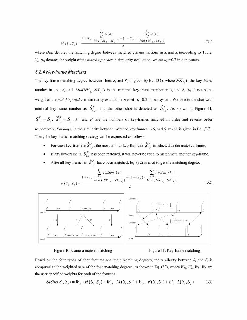
Given shot Si and Sj, if iSM is the number of camera motion types in Si from start frame to end frame,
we denote the shot with minimal number of camera motion types by MjiS ,
ˆ , and the other shot is denoted by MjiS ,
~. As Figure 10 illustrates, M
jiS ,ˆ =Si,
MjiS ,
~=Sj. We then will use M
jiS ,ˆ as the benchmark to find camera
motion matching in MjiS ,
~:
• For each camera motion in MjiS ,
ˆ , use Table 3 to find the closest matching motion in MjiS ,
~.
• If there is a motion in MjiS ,
~that exactly matches current camera motion in M
jiS ,ˆ (the matching degree
is 1), the current matching process will stop. • If there is no exact match for the current motion in M
jiS ,ˆ , the camera motion in M
jiS ,~
which has the largest matching degree is treated as the match.
• If any motion in MjiS ,
~ has been exactly matched with the motion in M
jiS ,ˆ , any other matching
operation will start from the next motion in MjiS ,
~.
• For any motion in MjiS ,
ˆ , start from the last exactly matched camera motion in MjiS ,
~ to seek the next
match. If there is no more camera motion in MjiS ,
~, the algorithm is terminated.
After the matching process, Eq. (31) is used to get the uniform camera motion matching degree. L+ and L- are
the number of camera motions matched “in order” and “in reverse order”, as shown in Figure 10.
2
),(
)()1(
),(
)(1
),(
11
jiji SS
L
kM
SS
L
kM
ji
MMMin
kD
MMMin
kD
SSM
∑∑−+
== ⋅−−+
=
αα (31)
where D(k) denotes the matching degree between matched camera motions in Si and Sj (according to Table.
3), αM denotes the weight of the matching order in similarity evaluation, we set αM=0.7 in our system.
5.2.4 Key-frame Matching
The key-frame matching degree between shots Si and Sj. is given by Eq. (32), whereiSNK is the key-frame
number in shot Si and ),(ji SS NKNKMin is the minimal key-frame number in Si and Sj. αF denotes the
weight of the matching order in similarity evaluation, we set αF=0.8 in our system. We denote the shot with
minimal key-frame number as FjiS ,
ˆ , and the other shot is denoted as FjiS ,
~. As shown in Figure 11,
iF
ji SS =,ˆ , j
Fji SS =,
~. F+ and F- are the numbers of key-frames matched in order and reverse order
respectively. FmSim(k) is the similarity between matched key-frames in Si and Sj which is given in Eq. (27). Then, the key-frames matching strategy can be expressed as follows:
• For each key-frame in FjiS ,
ˆ , the most similar key-frame in FjiS ,
~ is selected as the matched frame.
• If any key-frame in FjiS ,
~ has been matched, it will never be used to match with another key-frame.
• After all key-frames in FjiS ,
ˆ have been matched, Eq. (32) is used to get the matching degree.
2),(
)()1(
),(
)(1
),(
11
jiji SS
F
kF
SS
F
kF
ji
NKNKMin
kFmSim
NKNKMin
kFmSim
SSF
∑∑−+
== ⋅−−+=
αα (32)
Still ZOOM_IN Still
Shot Si
Still IRREGULAR PAN_RIGHT Still
Shot Sj
1.0 0.1 0.5 1.0
0 54 321
0 2 31
Keyframes…
Keyframes……
Shot Si
Shot Sj
Matched in order
Matched in inverse order
Figure 10. Camera motion matching Figure 11. Key-frame matching
Based on the four types of shot features and their matching degrees, the similarity between Si and Sj is
computed as the weighted sum of the four matching degrees, as shown in Eq. (33), where WH, WS, WF, WL are
the user-specified weights for each of the features.
),(),(),(),(),( jiLjiFjiMjiHji SSLWSSFWSSMWSSHWSSStSim ⋅+⋅+⋅+⋅= (33)

5.3 Group Level Similarity Evaluation
Based on Eq. (33), given a shot Si and a group Gj, the similarity between them is defined with Eq. (34).
jj GSjiji SSStSimMaxGSStGpSim
∈
= )},({),( (34)
This implies that the similarity between Si and Gj is the similarity between Si and the most similar shot in Gj.
In general, when we compare similarity between two groups using the human eye, we usually take the
group with fewer shot numbers as the benchmark, and then find whether there are any shots in the other
group similar enough to shots in benchmark group. If most shots in the benchmark group were similar
enough to the other group, they would be treated as similar, as shown in Figure 12. Therefore, given group Gi
and Gj, assume jiG ,ˆ indicates the group with fewer shot numbers, and jiG ,
~denotes the other group. Suppose
NT(x) denotes the number of shot in group x, then, the similarity between Gi and Gj is given by Eq. (35).
∑∈=
=)ˆ(
ˆ;1,
,
,
,
)~,()ˆ(
1),(ji
jii
GNT
GSijii
jiji GSStGpSim
GNTGGGpSim (35)
Hence, the similarity between group Gi and Gj is the average similarity between shots in the benchmark
group and their most similar shots in the other group.
G1
G2
Figure 12. Group similarity evaluation (the arrows indicate the most similar shots between G1 and G2)
5.4 Scene Level Similarity Evaluation
A video scene consists of visually similar groups, given two scenes SEi and SEj, the similarity between them
is derived from the similarity among the groups they contain. Assume Gi and Gj are the representative groups
in scenes SEi and SEj, then the similarity between SEi and SEj is given by Eq. (36).
)(Re);(Re),(),(
jjii SEpGroupSelectGSEpGroupSelectGjiji GGGpSimSESESeSim
==
= (36)
That is, the similarity between two scenes is the similarity between their representative groups.
5.5 Video Level Similarity Evaluation
Assuming NS(x) indicates the number of scenes in video x. Then, based on video similarity evaluation at the
scene level, Eq. (37), is used to evaluate the distance between two videos Vi and Vj.
)(,..,1,);(,..,1,)},({),(
jjliik VNSlVSEVNSkVSElkji SESESeSimMaxVVVdSim
=∈=∈= (37)

That is, the distance between Vi and Vj is the distance between the most similar scenes among them. Hence, if
videos Vi and Vj are very similar to each other, the similarity evaluated from Eq. (37) would be large;
however, if Vi and Vj are not similar to each other, their similarity may also be relatively large, since they
may contain just one similar scene. Hence, Eq. (37) is utilized as the first step for video similarity evaluation
to find those relatively similar videos, and then the similarity evaluation strategy at the scene, group and shot
levels is utilized to refine the retrieval result.
6. JOINT CONTENT HIERARCHY FOR PROGRESSIVE VIDEO ACCESS With the constructed video content hierarchy and the video similarity assessment at various levels, our video
browsing and retrieval can be integrated and with great benefit to both. The user can also refine his query by
progressively executing the browsing and retrieval processing. For example, the user executes the retrieval at
the video level, and then adopts Eq. (37) to find the similar video sequences. Since the semantic and low-
level features in the query video sequence may vary, it is relatively difficult to tell which part the user is
mostly interested in. Hence, by hierarchically browsing the content of the retrieved video sequences, the user
can refine his query by selecting a scene (or a group) as the query. Iterative execution operations guide the
user in finding the unit he is most interested in. In general, the progressive video content access strategy of
Insightvideo is executed as follows:
1. A hierarchical video browsing interface is first utilized to help the user browse, delivering an
overview of the video or video database, as shown in Figure 13. During video browsing, the user
may select any video unit as the query to query the database. That is, either the key-frame, group,
scene even the whole video may be selected as the query.
2. The user can also submit an example that is not in the database as the query. In that case, the video
analysis strategies are used to construct its content hierarchy. The hierarchical browsing interface is
utilized to help the user browse the content table of the query example and refine the query.
3. After the user has selected the query example, the system will utilize the similarity evaluation
scheme that corresponds to the same level as the query instance to find similar instances, and
present the results to the user, as shown in Figure 14. Users can click the “Up” or “Down” buttons to
view other retrieved units.
4. The user may also browse the content hierarchy of the retrieved video unit by double clicking. Then,
figure 15 will show the hierarchical content structure of the selected video unit. The first row shows
the summary of the current video, and all other rows illustrate the scene information in the video
(each row represents one scene). The row with the magnifier icon image on the left indicates that it
was ranked as one of the retrieved results. The user can click the magnifier icon image to browse
more details in the unit. Then, the user may select any unit in current interface as the new query. In
this way, the retrieval and hierarchical browsing capabilities are integrated to benefit each other in
helping the user to access the video content and refine his query efficiently.
5. Iteratively execute the step 3 and 4 until the user finds the satisfactory results or halts the current
retrieval operation at any time.

6.1 System Performance Two types of video retrieval results, retrieval at the shot level and video level, are executed in our system.
The experimental results are shown in Table 4 and Table 5 respectively. Our video database consists of 16
videos (about 6 hours) from various sources (5 film abstracts, 4 News and 7 medical videos). All videos were
processed with the techniques described above to extract their feature and content table. Then, InsightVideo
was used to hierarchical browse and progressively retrieve videos from the database.
While executing video retrieval at the shot level, two factors, precision and recall are defined to evaluate
the efficiency of the system. Precision specifies the ratio of the number of relevant shots to the total number
of returned shots. Recall specifies the ratio of the number of relevant video sequences found to the total
number of relevant video sequences in the database. While evaluating the similarity between shots, we set
WF, WM, WH and WL equal to 0.5, 0.1, 0.3 and 0.1 respectively. That is, we put heavy emphasis on the
matching of visual features. During the retrieval process, the relevant shots retrieved in the top 20 are
returned as the results. Performance is measured by comparing results produced by the assessment strategy
on the 5 queries for each type of video against human relevance judgment. From Table 4, we can see that our
system achieved rather good performance (76.8% in recall and 72.6% in precision) on different kinds of
video. However, since the camera motion, content and background of film abstracts are more complex than
other videos, the performance results of the film abstracts are somewhat worse. A more reliable and efficient
method may be needed for film evaluation.
Another experiment is executed to evaluate the efficiency of video similarity evaluation model at the
video level. In this experiment, each of 16 videos in the database is first manually separated into three nearly
equal clips (the entire video database contains 16×3=48 clips, no scene overlaps with the manually
segmented boundaries). Then, randomly select one clip from database as the query, and retrieve results from
the database. The ranks of the other two clips that are in the same video as the query are used to evaluate the
system performance.
We randomly select 24 retrieval results (with 8 for each), and show them in Table 4. To evaluate the
similarity between the videos, we set WF, WM, WH and WL equal to 0.4, 0.0, 0.5, 0.1 respectively. From Table
5, we see that our retrieval strategy achieved relatively good results, the average location of the retrieved
clips that are in the same video as the query is 4.27 (out of 47 clips, since the query clip is excluded from the
database). However, we find the retrieval results for News are worse than for the other two types of video.
This is because News programs are usually different from general video data: in common videos, a similar
scene may be shown repetitively in the video, however, in News program, most story units are reported only
once, hence, the three clips of the same News video may have large variety in content and visual features.
This can cause our system to falsely locate the related clips with the query example.

Figure 13. Hierarchical video content browsing Figure 14. Video retrieval interface
Figure 15. Content hierarchy of the retrieved result
Table 4. System retrieval performance at shot level (From top 20 results)
Content of the video database Shots in the video Recall Precision
Film Abstracts 526 0.62 0.65
News Programs 771 0.85 0.78
Medical Videos 1286 0.81 0.74
Average Performance 2583 0.768 0.726
Table 5. System retrieval performance at video level
Videos Query 1 Query 2 Query 3 Query 4 Query 5 Query 6 Query7 Query8 Medical videos 2 1 3 2 3 1 4 2 1 3 1 4 6 8 1 3 News program 6 7 5 3 7 11 8 3 7 2 4 7 8 13 4 12 Film Abstract 4 3 2 6 1 5 4 1 6 2 3 1 6 4 3 2
Average 4.27

7. CONCLUSION
In this paper we have presented the InsightVideo system, which constructs the video content hierarchy for
efficient video content access. A progressive video retrieval scheme is proposed which seamlessly integrates
hierarchical video browsing and retrieval. To create the video content table, several video analysis techniques
are introduced: (1) a statistical information based camera motion classification method, (2) a compressed
domain key-frame extraction method which is based on detected camera motions in each shot, and (3) video
group and scene detection and scene clustering strategies which organize the video content hierarchy. Video
similarity assessment at different levels (frame, shot, group, scene, video) is addressed. Based on constructed
video content hierarchy and the video similarity evaluation strategy, the hierarchical video browsing and
retrieval are seamlessly integrated together.
Unlike most other video retrieval systems that execute the video retrieval at the shot level, the retrieval
results of the InsightVideo are the units likely related to the query example in low-level features and
semantics. In contrast to other video browsing systems, we join the hierarchical video browsing with video
retrieval. This benefits both processes, and produces an effective progressive video retrieval system. The
features that distinguish our system from others are the following: (1) the integration of several novel video
processing techniques which improve existing algorithms in important ways, (2) constructing the video
content hierarchy allows the hierarchical video content browsing and summarization to be executed directly,
(3) addressing the video similarity at different levels to support the retrieval at various content levels, and (4)
a progressive retrieval which integrates the video browsing and retrieval processes, allowing users to shrink
and refine queries efficiently.
REFERENCES
1. H. J. Zhang, A. Kantankanhalli, and S.W. Smoliar. “Automatic partitioning of full-motion video”. ACM Multimedia system, 1(1), 1993.
2. H. J. Zhang, C.Y.Low, Stephen W. Smoliar, and D. Zhong, “Video parsing, retrieval and browsing: an integrated and content-based solution”, In proc. Of ACM int. conf. on Mlutimedia, 1995.
3. M. M. Yeung and B.-L. Yeo, “Video visualization for compact presentation and fast browsing of pictorial content”, IEEE Transaction on CSVT, Vol.7, pp.771-785, Oct. 1997.
4. J. R. Smith, “VideoZoom spatio-temporal video browser”, IEEE Trans. on Multi. vol. 1, No.2, 1999. 5. Y.Alp Aslandogan and Clement T. Yu, “Techniques and Systems for Image and Video Retrieval”, IEEE
Trans. On Knowledge and Data Engineering, Vol.11, No. 1, 1999. 6. D.W. Howard, K. Takeo, A.S. Michael and M.S. Scott, “Intelligent Access to Digital Video: Informedia
Project”, IEEE computer, vol. 29, No.5, May 1996 7. S.F. Chang, W. Chen, H.J. Meng, H. Sundaram and D. Zhong, “VideoQ: an automated content based
video search system using visual cues”, Proc. of 5th ACM inter. Conf. on Multi., 1997,Pages 313 – 324. 8. A. Hampapur, A. Gupta, B. Horowitz, C-F. Shu, C. Fuller, J. Bach, M. Gorkani, R. Jain, “Virage Video
Engine”, SPIE Vol. 3022, 1997. 9. A. Pentland, R. Picard, and S. Sclaroff, “Photobook: Content-based manipulation of image database”,
Int. J. Computer vision, Vol. 18, pp.233-254, 1996. 10. J.R. Smith and S.F. Chang, “VisualSEEk: A Fully Automated Content-Based Image Query System”,
Proc. ACM Multimedia conf. Pp. 87-98, Boston, 1996.

11. V.E. Ogle and M.Stonebraker, “Chabot: Retrieval from a Relational Database of Image”, Computer, Vol. 28, No. 9, Sept. 1995.
12. C. Faloutsos, W. Equitz, M. Flickner, W. Niblack. S. Petkovic, and R. Barber, “Wfficient and effective querying by image content”, J. Intell. Inf. System, vol. 3, pp.231-262, 1994.
13. H. Jiang, A. Elmagarmid, “WVTDB-A Semantic Content-Based Video Database System on The World Wide Web”, IEEE Transactions on Knowledge and Data Engineering, Vol 10, No. 6, 1998.
14. A. Elmagarmid, et al., “Video Data Bases: Issues, Products and Applications”, Kluwer Academic press, Mar. 1997.
15. S.F. Chang, J.Smith, and J. Meng, “Efficient Techniques for Feature Based Image/Video Access and Manipulation”, Proc. 33rd Ann. Clinic on Library Application of Data Processing Image Access and Retrieval, Mar. 1996.
16. M. La Cascia and E. Ardizzone, “JACOB: Just A Content-Based Query System for Video Database”, Proc. ICASSP, Atlanta, 1996.
17. J.R. Smith and S.F. Chang, “Searching for Images and Video on the World-Wide Web”, CTR technical Report No. 459-96-25, Columbia University, Aut. 1996.
18. D.W. Howard, K. Takeo, A.S. Michael and M.S. Scott, “Intelligent Access to Digital Video: Informedia Project”, IEEE computer, vol. 29, No.5, May 1996
19. B.L. Yeo, B. D. Liu, “Rapid scene analysis on compressed video”, IEEE Trans. on CSVT, vol. 5, No.6, pp.533-544, Dec. 1995
20. J. Fan, W. Aref, A. Elmagarmid, M. Hacid, M. Marzouk, X. Zhu, “MultiView: Multilevel video content representation and retrieval”, Journal of Electronic imaging, 10(4):895-908, oct., 2001.
21. R. Szeliski, Video mosaics for virtual environments. IEEE Computer Graphics and Application, pp.22-30 , March 1996.
22. C.W. Ngo, T.C. Pong, H.J. Zhang and R.T. Chin, “Motion characterization by temporal slice analysis”, in Proc. of Computer Vision and Pattern Recognition, vol. 2, pp.768-773, 2000.
23. W. Xiong, J. Chung-Mong Lee: “Efficient Scene Change Detection and Camera Motion Annotation for Video Classification”. Computer Vision And Image Understanding, Vol.71, pp.166-181, 1998.
24. M.V. Srinivasan, S. Venkatesh and R. Hosie, “Qualitative Estimation Of Camera Motion Parameters From Video Sequences”, Pattern Recognition, 30(4):593-606,1997.
25. R.C Jain, “Direct computation of the focus of expansion”, IEEE Trans. on PAMI, 5(1):58-64, Jan, 1983. 26. Y.P. Tan, Saur D.D., Kulkami S. R., Ramadge P.J. “Rapid estimation of camera motion from
compressed video with application to video annotation”, IEEE Trans. on CSVT, 10(1):133-146, 2000. 27. V. Kobla, D.S. Doermann and A. Rosenfeld, “Compressed domain video segmentation”, CfAR technical
report CAR-TR-839 (CS-TR-3688), 1996. 28. C. Dorai, and V. Kobla, “Perceived visual motion descriptors from MPEG-2 for content-based HDTV
annotation and retrieval”, in Proc. of IEEE 3th Workshop on Multimedia Sig. Pro., pp.147-152, 1999. 29. A. Hanjalic and H. J. Zhang, “An integrated scheme for automated video abstraction based on
unsupervised cluster-validity analysis”, IEEE Trans. on CSVT, 9(8):1280-1289, 1999. 30. H. J. Zhang, J. Wu, D. Zhong and S.W. Smoliar, “An integrated system for content-based video retrieval
and browsing”, Pattern recognition, 30(4):643-658, 1997. 31. Y. Zhang, Y. Rui, T.S. Huang, and S. Mehrotra, “Adaptive key frame extraction using unsupervised
clustering”, In Proc. of ICIP, vol. 1, pp.866-870, Chicago, 1998. 32. Wayne Wolf, “Key frame selection by motion analysis”, in Proc. IEEE ICASSP, pp.1228-1231, 1996. 33. A. Pentland, R.Picard, G.Davenport, and K. Haase, “Video and image semantics: advanced tools for
telecommunications”, IEEE multimedia magazine, pp.73-75, summer, 1994. 34. Y. Avrithis, N. Doulamis, A. Doulamis, S. Kollias, “Efficient content representation in MPEG video
database”, In proc. IEEE workshop on content based access of image and video database, pp.91-95, Santa Barbara, 1998.
35. B. Shahraray and D.C. Gibbon, “Automatic generation of pictoral transcripts of video programs”, In proc. of IS&T/SPIE Digital video compression: Algorithms and Technilogies, pp.512-519, 1995.
36. T. Lin, H.J. Zhang “Automatic Video Scene Extraction by Shot Grouping”, in Proc. of ICPR 2000.

37. Y. Rui, T. Huang, S. Mehrotra, “Constructing table-of-content for video”, ACM Multimedia Systems Journal, Special Issue Mult. Systems on Video Libraries, 7(5):359-368, Sept, 1999.
38. M. M. Yeung, B. L. Yeo, “Time-constrained clustering for segmentation of video into story units”, in Proceedings of ICPR’96.
39. W. Zhou, A. vellaikal, C. J. Kuo, “Rule-based video classification system for basketball video indexing”, In Workshop of 9th ACM Multimedia conf., Los Angeles. 2001.
40. D. Swanberg, C.F. Shu, R. Jain, “Knowledge-guided parsing in video database”, in Proc. of IS&T/SPIE Storage and Retrieval for Image and Video Databases II, San Jose, 13-24, 1993.
41. X. Zhu, L. Wu, X. Xue, X. Lu, J. Fan. "Automatic Scene Detection in News Program by Integrating Visual Feature and Rules", Proc. of 2nd IEEE PCM Conf., LNCS2195, pp.837-842, Beijing, 2001.
42. D. Zhong, H. J. Zhang and S.F. Chang, “Clustering methods for video browsing and annotation”, Technical report, Columbia Univ.,1997.
43. D.A.Adjeroh, M.C.Lee and I. King “A Distance Measure for Video Sequence Similarity Matching”, in Proc. of International workshop on Multimedia Database Management Systems, 1998.
44. N. Dimitrova, M. Abdel-Mottaled, “Content based Video Retrieval by Example video clip”, in Proc. of SPIE Vol.3022, 1998.
45. R. Lienhart, W. Effelsberg and R. Jain, “VisualGREP: A systematic method to compare and retrieval video sequences”, In:SPIE vol.3312, 1997, 271-282
46. L. Zhao, W. Qi, S. Z. Li, S. Yang, H. Zhang “Key-frame Extraction and Shot Retrieval Using Nearest Feature Line (NFL)”, Proc. on ACM multimedia workshops, pp. 217 – 220, 2000.
47. S. Li, J. Liu, “Face Recognition Based on Nearest Linear Combinations”, IEEE Trans. On Neural Networks, 10(2):439-443, March 1999.
48. X. Liu, Y. Zhuang and Y. Pan, “A new approach to retrieve video by example video clip”, in Proc. of the 7th ACM Multimedia Conf., pp.41-44, 1999.
49. A.K. Jain, “Algorithms for clustering data”, Prentice Hall, 1998. 50. A. Hauptmann, M. Witbrock, “Story Segmentation and Detection of Commercials in Broadcast News
Video", ADL-98 Advances in Digital Libraries Conference, Santa Barbara, CA., April 22-24, 1998 51. C. Ngo, T. Pong, H. Zhang, “On clustering and retrieval of video shots”, in Proc. of 9th ACM Multimedia
Conf., pp.51-60, 2001. 52. J. Fan, J. Yu, G. Fujita, T. Onoye, L. Wu, I. Shirakawa, “Spatiotemporal segmentation for compact video
representation”, Signal processing: Image communication, vol.16, pp.553-566, 2001. 53. E. Ardizzone, M. Cascia, A. Avanzato, A. Bruna, “Video indexing using MPEG motion compensation
vectors”, in Proc. of IEEE Conf. on Multimedia Computing and Systems, Florence, Italy, 1999. 54. A. Divakaran, R. Radhakrishnan, K. Peker, “Motion activity-based extraction of key-frame from video
shots”, in Proc. of IEEE ICIP Conf., Rochester, New York, 2002. 55. A. Divakaran, R. Radhakrishnan, K. Peker, “Video summarization using descriptors of motion activity:
A motion activity based approach to key-frame extraction from video shots”, Journal of Electronic Imaging, 10(4):909-916, 2001.
56. M. Lazarescu, S. Venkatesh, G. West, “On the automatic indexing for cricket using camera motion parameters”, in Proc. of IEEE ICME Conf., Laussane, Switzerland, 2002.
57. S. Jeannin, A. Divakaran, “MPEG-7 visual motion descriptor”, IEEE Trans. on CSVT,11(6):720-724, 2001.
58. B.S. Manjunath, P. Salembier, T. Sikora, Introduction to MPEG-7: Multimedia Content Description Interface, Wiley, June 2002.
59. The MPEG-7 visual part of the XM 4.0, ISO/IEC MPEG99/W3068, Maui, USA, Dec., 99.


![Towards Hierarchical Scheduling in VxWorksrbril/publications/[Behnam et al 08].pdf · Towards Hierarchical Scheduling in VxWorks ∗ Moris Behnam†, Thomas Nolte, Insik Shin, Mikael](https://img.dokumen.tips/doc/110x75/5e6fa360fb4f7f5dbc46c773/towards-hierarchical-scheduling-in-rbrilpublicationsbehnam-et-al-08pdf-towards.jpg)