Embed Size (px)
Citation preview

INSIDE AND OUTSIDE LIQUIDITY
Bengt Holmström1 Jean Tirole2
August 30, 2010 (edited version forthcoming at MIT Press)
1MIT, [email protected] School of Economics, [email protected].
Outline
OUTLINE
Acknowledgements
Prologue
PART I: Basics of leverage and liquidity
Chapter 1. Leverage.
Chapter 2. A simple model of liquidity demand.
PART II: Complete markets
Chapter 3. Aggregate liquidity shortages and liquidity premia.
Chapter 4. A Liquidity Asset Pricing Model (LAPM).
PART III: Public provision of liquidity
Chapter 5. Public provision of liquidity in a closed economy.
Chapter 6. Is there still scope for public liquidity provision when firms have access to
global capital markets?
PART IV: Waste of liquidity and public policy
Chapter 7. Financial muscle and overhoarding of liquidity .
Chapter 8 Specialized inputs and secondary markets.
Epilogue: Summary and concluding thoughts on the subprime crisis
Inside and Outside Liquidity 1

Acknowledgements
Acknowledgements
The idea of writing this book on inside and outside liquidity started when we were
invited to give the Wicksell lectures at the Stockholm School of Economics in 1999. We
are grateful for and honored by this invitation, which gave us the impetus for thinking
more deeply about the implications of the framework we developed in the mid-1990s.
As usual, our own contribution builds on the shoulders of many others, from the classic
works of Wicksell, Keynes, Hicks on liquidity and government macroeconomic policy to
the modern corporate finance literature, which we take as the foundation for our modeling
approach. We are very grateful to the many researchers whose work is cited here, and
apologize for any omission which, we are certain, will have arisen.
We have benefitted greatly from the insights and the inputs of many researchers: Jean-
Charles Rochet, Emmanuel Farhi, Gary Gorton and Tri Vi Dang with whom we have
collaborated on related topics and who have generously shared their thoughts with us;
Pablo Kurlat, who proof-read an early version of the book and provided excellent research
assistance; IvanWerning, who corrected an error in our 1998 paper (see chapter 3); Arvind
Krishnamurthy for constructive criticism of earlier drafts and Daron Acemoglu, Tobias
Adrian, Bruno Biais, Olivier Blanchard, Jeremy Bulow, Ricardo Caballero, Douglas Di-
amond, Gary Gorton, Olivier Jeanne, Anyl Kayshap, Nobu Kiyotaki, Guido Lorenzoni,
Thomas Mariotti, Ernesto Pasten, Andrei Schleifer, Jeremy Stein, Robert Townsend,
Robert Wilson and Mark Wolfson for extensive conversations on the subject.
Needless to say, we are entirely responsible for any mistake that remain (comments
can be addressed to us at [email protected] or [email protected]).
Besides the Stockholm School of Economics, drafts of this book were taught to several
generations of students at MIT, Toulouse, Wuhan University, University of Chicago, and
the New Economic School, Moscow. We thank all the participants for helpful feedback.
Inside and Outside Liquidity 2
Acknowledgements
Our assistants Emily Gallagher and Pierrette Vaissade did a great job typing the
manuscript, always in good cheers; they deserve our sincere gratitude.
We are grateful to our editor. . . . and to. . . for typesetting and editing the manu-
script. . . ..
MIT and TSE provided us with friendly and very stimulating research environments
during all those years. One cannot underestimate the benefits of conversations and com-
ments gleaned in corridors, at the coffee machine and seminars. As always, they played a
role in the conception of this book. While these research environments owe much to the
researchers that make them intellectually exciting, they would not exist without gener-
ous external support. Jean Tirole is extremely grateful to the partners of the Toulouse
School of Economics (TSE) and of the Institut d’Economie Industrielle (IDEI) for their
commitment to funding fundamental research; this in particular includes partners re-
lated to finance and macroeconomics: Banque de France, which has taken a particularly
keen interest in research on liquidity, and also AXA, BNP Paribas, Caisse des Dépôts
et Consignations, Crédit Agricole, Exane, Fédération Française des Banques, Fédération
Française des Sociétés d’Assurance, Financière de la Cité, Paul Woolley Research Initia-
tive and SCOR. Bengt Holmström thanks the Yrjö Jahnsson Foundation for support and
Anyl Kayshap for the invitation to visit the Initiative on Global Markets at the University
of Chicago in the Fall 2006, and John Shoven for the invitation to visit Stanford Institute
of Economic Policy Research (SIEPR) in the Spring 2010. Some of the work on the book
was done during these visits.
Finally, our families and in particular our wives Anneli and Nathalie provided much
understanding and love during the long gestation of this book.
Inside and Outside Liquidity 3
Prologue
Prologue: Motivation and roadmap
Why do financial institutions, industrial companies and households hold low-yielding
money balances, Treasury bills and other short-term assets? The standard answer to
this question, dating back at least to Keynes (1936), Hicks (1967) and Gurley and Shaw
(1960), is that these assets are “liquid” as they allow their owners to better weather
income shortages.∗
It is unclear, though, why an economic agent’s ability to withstand shocks would not
be better served by the broader concept of net wealth, including stocks and long-term
bonds. While some forms of equity, such as private equity, may not be readily sold
at a “fair price,” many long-term securities are traded on active organized exchanges;
for example, liquidating one’s position in an open-ended S&P 500 index fund can be
performed quickly and at low transaction costs. For some reason a big part of the agents’
net wealth is not liquid. It cannot be used as a substitute for liquid assets, explaining
why the yield on liquid assets is lower than could be expected from standard economic
models (the “risk-free rate puzzle”). The standard theory of general equilibrium offers no
explanation for this phenomenon. In the Arrow-Debreu model, and its variants, economic
agents are subject to a single budget constraint, implying that the consumers’ feasible
consumption sets and the firms’ feasible production sets only depend on their wealth.
Similarly, financial institutions and industrial companies pay a lot of attention to
risk management. They hedge against liquidity risks using short-term securities, credit
facilities, currency swaps and similar instruments, adjusting their positions to meet future
liquidity needs in the most efficient way. These activities cost billions of dollars. Yet,
received theory is not of much help in explaining all the resources and attention spent
on them. In an Arrow-Debreu world, it does not matter whether economic agents make
∗The book’s title "Inside and Outside Liquidity" paraphrases Gurley and Shaw’s (1960) "inside andoutside money," which distinguishes claims that private parties have on each other versus claims that
private parties have on government. Our usage is consistent with this distinction. Wicksell (1898) was
one of the first authors to emphasize the dual role of money as a store of value and a medium of exchange.
Inside and Outside Liquidity 4
Prologue
their consumption and production plans at the initial date or make these decisions later
on provided that they can contract on transfers of numéraire from one period to the
next (Arrow 1970). In particular, the Modigliani-Miller (1958) irrelevance results imply
that the hoarding of liquidity or the hedging of liquidity risk (through choice of leverage,
dividend payments, etc.) do not affect a firm’s value.
The purpose of this monograph is to offer an explanation of the demand for and
supply of liquid assets using insights from modern corporate finance and to study how
such a theory can explain the pricing of assets, the role of liquidity management, real
investments and also how this theory relates to some classic themes in macroeconomics
and in international finance.
Macroeconomic policy rests on the presumption that the government can do things
that the market cannot. Foremost among these is the provision of liquidity. The govern-
ment provides liquidity in a variety of ways: through industry and banking bailouts, de-
posit insurance, the discount window, open-market operations, implicit insurance against
major accidents or epidemics, unemployment insurance, social security, debt management
and so forth. The result is often a redistribution of income from consumers to producers
or from future generations to current ones. The Ricardian equivalence theorem (Barro,
1974), the macroeconomic counterpart of the Modigliani-Miller theorem, suggests that
these activities are useless, since economic agents can replicate privately optimal out-
comes by undoing whatever the government does.
In this monograph we will depart from the Arrow-Debreu paradigm in one single,
but important way: we will assume that some part of a firm’s income stream cannot
be promised or pledged to investors. The implication is that the income base on which
various kinds of financial claims can be built, is smaller than in the Arrow-Debreu world.
For the most part, we will assume that the only imperfection in the economy is the non-
pledgeability of some part of the investment income. On the pledgeable part arbitrary
financial claims can be written.
Inside and Outside Liquidity 5
Prologue
There are several reasons why some of the income from investments would be non-
pledgeable. One reason is that some agents may not participate in markets; indeed,
they may not even be born, as in the case of future generations. This type of market
incompleteness has been thoroughly investigated in the overlapping-generations literature,
starting with Allais (1947), Samuelson (1958) and Diamond (1965).
A second reason is that information is imperfect and therefore the potential set of
financial claims is reduced. Consumers can pledge only a small share of their future labor
income, for institutional reasons (limited liability, limited slavery, priority of tax claims),
verifiability problems (a liability-ridden individual may move abroad), and incentive con-
siderations (future income is endogenous). Similarly, individual investors must share
firms’ proceeds with insiders (large shareholder, managers, employees) either because the
latter enjoy perks, can divert resources or may exert insufficient effort, or because insiders
must be given a share of the created resources to refrain from engaging in moral hazard.
Adverse selection further limits the extent to which firms can market their future income
to investors.
A key implication of non-pledgeability is that firms (as well as consumers) can count
on liquidating only part of their wealth whenever they need funds. Instead, they must
prepare themselves for adverse financial shocks by hoarding liquid assets or by contracting
in other ways for the provision of liquidity. Firms are willing to pay a premium for liquidity
services. We will show that in general they have to do so, because the supply of liquid
assets is also constrained by the fact that the returns from productive activities cannot
be fully pledged. Non-pledgeability reduces the amount of wealth in the economy, which
in turn limits the ability of investors to promise, in a credible manner, future financing of
firms. This observation gives rise to a demand for stores of value that can transfer wealth
from today to tomorrow as well as across states of nature tomorrow. One of the basic
questions we will address in this book is this: When is the corporate sector of the economy
liquidity constrained in the sense that the wealth it produces is insufficient to meet its
Inside and Outside Liquidity 6
Prologue
future liquidity needs? We refer to this case as a shortage of inside liquidity. This shortfall
will to some extent be satisfied by two sources of outside liquidity: the government and
international financial markets. In general, neither source will be sufficient and there will
be a shortage of aggregate liquidity. This in turn will have interesting implications for how
the government supplies and manages liquidity as well as liquidity management within
firms.
The monograph is organized as follows. Part I of the book builds the foundations
for the corporate demand for liquidity. Chapter 1 introduces a simple model of credit
rationing with constant returns to scale. Credit rationing of some kind is essential for cor-
porate liquidity demand. Chapter 2 introduces the workhorse model of liquidity demand
that we will use throughout the book. In this model, firms with limited pledgeability
must plan their liquidity in advance. Firms demand liquidity because they want to insure
themselves against credit rationing. Through mechanisms such as credit lines or credit
default swaps, investors commit themselves to supplying funds in states of nature in which
they would not naturally have done so, i.e. in states in which liquidity needs exceed the
future income that can be pledged to investors. We also examine the provision of liquid-
ity by investors who cannot perfectly monitor the use that is made of the corresponding
funds.
Chapter 2 also compares our model of corporate liquidity demand with the celebrated
model of consumer liquidity demand by Bryant (1980) and Diamond-Dybvig (1983).
While the two types of models differ in many respects, we show that there is a close
formal relationship between them as well. Furthermore, the two can readily be merged
into a single framework in which corporations and consumers compete for liquidity.
Part II of the book (chapters 3 and 4) considers the benchmark of complete markets:
While there is a wedge between value and pledgeable income, the latter is traded on
efficient, complete markets. The economy is then an Arrow-Debreu economy, except for
the limited pledgeability. Complete markets imply that liquidity may be scarce, but is
Inside and Outside Liquidity 7
Prologue
allocated efficiently.
Chapter 3 asks whether the private sector provides enough aggregate liquidity on
its own. That is, do the firms in the aggregate create enough pledgeable income — inside
liquidity — to support the financial claims necessary for implementing a second-best, state-
contingent production plan. The answer is yes if the corporate sector is a net borrower
and the firms’ liquidity shocks are idiosyncratic. In that case the second best plan can be
implemented by each firm holding a share of the market index. On the other hand, if the
corporate sector is a net lender there will always be a shortage of aggregate liquidity. The
same is true if all firms are hit by the same (macroeconomic) shock or more generally if
macroeconomic shocks are sufficiently large relative to the idiosyncratic shocks.
A shortage of stores of values induces the private sector to try to create more, albeit
at a cost. What is in short supply is not non-contingent liquidity, but liquidity in those
states of nature in which the economy is doing poorly, and, as we later point out, the
state has a comparative advantage in creating such contingent liquidity. Creation of more
“parking space” by the private sector may involve investing in projects that deliver a safe
income, more costly choices of governance that raise the corporations’ pledgeable income —
such as going public or resorting to monitoring structures, or costly financial innovations
that enable a more efficient use of collateral. Examples of the latter include bilateral
and tri-party repos (legal innovations that free posting of collateral from the vagaries of
bankruptcy processes), and securitization, which transforms illiquid, low grade loans into
publicly traded assets of higher quality. Our approach thus fits well with de Soto (2003)’s
view that a major role of a financial system is to transform “dead capital” into “live
capital”. He thought of the opportunities to create collateral in developing economies.
What seems to take place at the beginning of the new century was excesss savings from
China and other developing countries with underdeveloped financial markets, finding their
way to developed countries, and especially the U.S., which could meet the demand for
parking space at a lower cost.
Inside and Outside Liquidity 8
Prologue
When there is insufficient inside liquidity, financial instruments that originate outside
the private sector — outside liquidity — can improve productive efficiency by facilitating
access to liquidity and by lowering the cost of it. Prime suppliers of outside liquidity are
the government and international financial markets.
Chapter 4 shows how to compute asset prices using the analog of Arrow-Debreu state-
contingent prices, but assuming that only pledgeable income can be used as the basis for
contingent claims.† While the basic logic of our Liquidity Asset Pricing Model (LAPM)
is identical to that of the Arrow-Debreu model, LAPM prices do not merely reflect the
yield of the assets, but also the value that they bring by helping firms withstand liquidity
shocks. The chapter also illustrates how one can use state prices to derive an optimal
policy for risk management at the firm level.
Thus Part II of this monograph assumes that liquidity is dispatched efficiently through
explicit or implicit state-contingent claims on all pledgeable income. The analysis of
complete markets derives, in a sense, an upper bound on the available liquidity. In practice,
liquidity may not be properly redispatched from economic agents who end up having an
excess of it to those in need of liquidity. Put differently, efficient contracts for redispatching
liquidity may not have been signed. Parts III and IV study two such situations. In the
first, analyzed in Chapter 5, consumers are unable to directly pledge their future income
to firms, at least in states of nature where the latter are short of liquidity; we interpret
public provision of liquidity as the government filling the corresponding gaps and using its
taxation power to transfer income from consumers to firms in bad macroeconomic states.
In the second situation, studied in Chapters 7 and 8, the lack of coordination occurs
within the corporate sector.
Chapter 5 argues that the state, through its regalian taxation power, can increase the
†Geanakoplos, in a series of papers, has emphasized the essential role of collateral in financial mar-kets and studied in general equilibrium models the optimal assignment of collateral asset pricing (see
Geanakoplos, 1996 and Geanakoplos et. al., 1995). The methods he uses and the questions he asks are
different from ours, but the general context and perspective are related.
Inside and Outside Liquidity 9
Prologue
pledgeability of consumers’ future income and thereby create liquidity for the corporate
sector. Consumers and firms can be made better off by having the government act as
an insurance broker, transferring funds from consumers to firms when the latter are hit
by aggregate liquidity shocks. We study government policy assuming that an explicit
insurance contract can be drawn up ex ante, but argue that a number of ex post policy
interventions emulate the patterns of optimal government insurance. The ability of the
government to provide liquidity ex post, gives it a potential advantage over privately
supplied liquidity. Privately supplied liquidity often requires ex ante investments in short-
term assets, incurring an opportunity cost whether liquidity is needed or not. By contrast,
an ex post government policy that does not waste liquidity can be much cheaper, especially
when covering liquidity shortages that occur rarely.
Chapter 6 pursues the analysis of public provision of liquidity by asking whether the
presence of efficient international financial markets might eliminate all potential liquidity
shortages. The answer is no in general. A country’s access to international financial
markets is limited by its ability to generate pledgeable income that is tradable. We study
the relationship between international and domestic liquidity in an open economy with
both tradable and non-tradable goods and conclude that when there is a shortage of
international liquidity, the insights about the value of domestic liquidity continue to hold.
Chapters 7 and 8 depart from perfect coordination within the corporate sector and
looks at situations in which each firm individually arranges its own supply of liquidity
without any ex ante coordination with the other firms. The only type of coordination
occurs ex post in spot markets which can reallocate liquidity. One may ask how close
this kind of self-provided liquidity arrangement comes to the second-best. We show that
it will in general not replicate the second-best optimum, because firms may hoard either
too much or too little liquidity. Nevertheless, the government may be unable to improve
on the situation in contrast to the large literature on incomplete insurance markets.
The epilogue summarizes the main lessons to be drawn from our particular approach
Inside and Outside Liquidity 10
Prologue
towards the supply of inside and outside liquidity and relates it to the subprime crisis.
On terminology: Throughout this book, we will take the terms pledgeable income, liq-
uidity and collateral to mean the same thing and use them interchangably.‡ The financial
crisis that began in 2007 we shall call the subprime crisis for brevity.
‡Clearly, collateral can be different from pledgeable income in many contexts. The value of the assets
backing up debt is often higher than the value of debt (the debt is over-collateralized). This may be
because the underlying assets are risky and do not protect the investor’s claim in all states of nature. Or
it may be, because the value of collateral is worth less to the investor than it is to the borrowing firm.
Note that even if the collateral is worth very little to the investor it can provide proper incentives for
repayment of debt as long as the borrower prefers to repay the debt than lose his collateral and has the
means to do so.
In our complete market model, the amount of collateral is exactly equal to the amount promised in any
given state. Considerations of default are already built into the notion of pledgeable income and will not
happen in equilibrium. Promising more than the pledgeable income would not be credible and promising
less would waste collateral.
Inside and Outside Liquidity 11
Part I
BASICS OF LEVERAGE
AND LIQUIDITY
12

Introduction
Introduction
In standard microeconomic theory, a firm that confronts financial needs can meet them
as they arise by taking out loans or by issuing new securities, whose repayments and
returns are secured by the cash flows that the firm generates. As long as the net present
value of a re-investment is positive, investors are willing to supply the needed funds.1
Reality seems very different. Firms keep a close watch on their current and forecasted
cash positions, making sure that their essential liquidity needs can be met at all times.
They do not wait until the cash register is empty. To guard against liquidity shortages,
firms arrange financing in advance using both the asset and the liability sides of their
balance sheets. On the asset side they may hoard liquidity by buying Treasury bills and
other safe assets that can be easily sold when necessary.2 On the liability side, they may
take out credit lines or issue securities that give them flexibility in their management of
cash, such as long-term debt, preferred equity and straight equity.3 The recent subprime
crisis is a vivid demonstration of how costly — and in some cases impossible — it can
be to face a maturity mismatch and to seek financing in times of distress. Financial
institutions have been struggling to replace the short-term, market-based financing that
they had grown used to in boom times with alternative sources of funding. At the same
time they have been forced to delever significantly by selling assets at distressed prices.
The troubles in the financial sector in turn have shut off normal credit channels for the
non-financial sector, causing bankruptcies and distress throughout the economy. A crisis
of this magnitude is obviously rare, but it certainly is a stark reminder of how important
1In the case of a debt overhang, additional financing will require that previous contracts are renego-
tiated.2Some non-financial firms hold surprising amounts of liquid assets at any given time. Big technology
firms like Microsoft and Nokia have at times held billions of dollars in liquid instruments, mostly, if
not exclusively, in the form of safe, low-yielding debt. Large accumulations of cash like this provide a
readiness to make major acquisitions, but also a hedge against liquidity shocks.3Brunnermeier and Pedersen (2009) talk about funding liquidity when the liability side is used and
market liquidity when the asset side is used.
Inside and Outside Liquidity 13
Introduction
it is to think about one’s liquidity needs in advance rather than wait until the need
materializes.
By now there are several related theories in modern corporate finance that can ex-
plain why firms demand liquidity. Each theory provides a reason why a firm wants to buy
insurance against higher credit costs or outright credit rationing, stemming from infor-
mation problems. In von Thadden (2004), a firm that waits may be unable to get access
to funding due to adverse selection problems. Adverse selection can make it very costly
for a firm to obtain funding and in the worst case, asset and credit markets may dry up
entirely.4 “Signal-jamming” is an alternative rationale for advanced funding (e.g., Bolton
and Scharfstein,1990 and Fudenberg and Tirole, 1985). If financiers base tomorrow’s re-
financing decision on a firm’s current performance, competitors have an incentive to prey
on each other by choosing hidden actions, such as secret price cuts, that hurt rivals and
makes them look financially weak. In equilibrium, the market can see through this, but
nevertheless the wasteful signaling behavior is rational. To prevent such predation, a firm
has an incentive to secure its funds in advance (in a publicly observable fashion).
Throughout this book, we will employ a very simple information-based model as the
driver of liquidity demand. The key assumption is that firms are unable to pledge all of
the returns from their investments to the investors. Insiders, from control shareholders to
managers to ordinary employees, enjoy private benefits of various kinds that create a wedge
between total returns and pledgeable returns. The insiders may consume employment
rents, enjoy perks, engage in empire building, or receive inducements to perform that
give them an extra share of the firm’s payoff. To the extent these private benefits cannot
4The idea that adverse selection may lead to market freezes dates back to Akerlof (1970). Some recent
papers have used Akerlof’s model to show how the inability to sell legacy assets may hamper reinvestment
policies: see e.g., House and Masatlioglu (2010) and Kurlat (2010). Philippon and Skreta (2010) and
Tirole (2010) study how the state can jumpstart asset markets when financial institutions can opt to be
refinanced in a (cleaned-up) financial market instead. Daley and Green (2010) show how the thawing of
an illiquid market is affected by the accrual of news about the quality of individual assets and by the
waiting strategies of sellers who try to signal a high quality of their assets by conveying the message that
they are not particularly eager to part with them.
Inside and Outside Liquidity 14
Introduction
be transferred or paid for up front, a part of the total surplus will not be pledgeable to
outside investors.
This partial non-pledgeability of investment returns can make it more costly or im-
possible to finance a project. And even when the project can get off the ground, private
benefits can make reinvestments difficult in the future. In general, as we will show, firms
will face credit rationing both at the start as well as the future. There is however a key
difference between credit rationing at the initial financing stage and at the refinancing
stages: in the latter case, credit rationing can be anticipated and therefore measures
can be taken to insure against it. In other words, private benefits create a demand for
liquidity.
We start by showing (in chapter 1) how a simple moral hazard model with limited
liability can give rise to a wedge between total and pledgeable income. Chapter 2 intro-
duces a “liquidity shock” that may hit the firm after it has sunk its initial investment.
This gives rise to a demand for liquidity. We show that if the potential liquidity shock
is severe enough, the firm needs to arrange financing in advance or face costly credit
rationing. Firms face both a solvency concern (the need to be adequately capitalized in
order to attract financing in the first place) and a liquidity concern (the risk of facing
solvency concerns in the future). The optimal design exhibits a trade-off between liquid
and illiquid investments: the higher the insurance purchased by the firm in the form of
a liquidity backup, the lower the investment in illiquid assets. Put differently, the firm
can opt for a large scale together with an important maturity mismatch (much long-term
illiquid assets and little short-term liquidity), or for a smaller, but more secure balance
sheet.
Appendix 2.1 shows how private information about the magnitude of the liquidity
shock limits contracting possibilities and affects the optimal solution and the demand for
liquidity. Appendix 2.2 addresses an obvious question: how our model of liquidity demand
by firms compares with the more extensively studied case of consumer liquidity demand.
Inside and Outside Liquidity 15
Introduction
Our main approach is to assume that parties can write fully state-contingent, enforce-
able contracts on all pledgeable income; that is, there is a complete market for state-
contingent claims on the pledgeable part, while no contracts can be made on the private
part of income. The virtue of this (unrealistic) assumption is that it makes the model
very tractable and provides a rather disciplined modeling approach. The imperfection we
explore is a minimal deviation from the world of complete markets. Had one assumed
a more general incomplete market structure, whether exogenously or endogenously, the
options would be many and harder to choose from.
Inside and Outside Liquidity 16
Chapter 1
Leverage
1.1 A simple model of credit rationing with fixed in-
vestment scale
We will use a very simple model of credit rationing as the basic building block for our
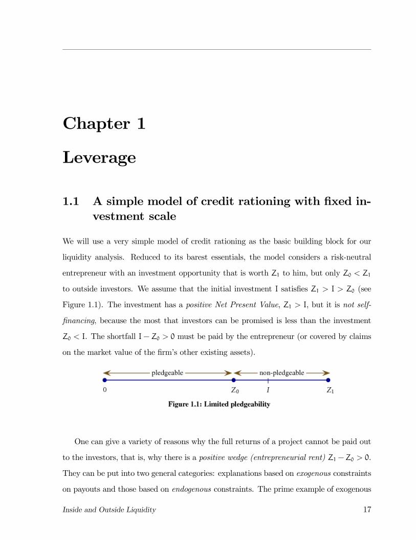
liquidity analysis. Reduced to its barest essentials, the model considers a risk-neutral
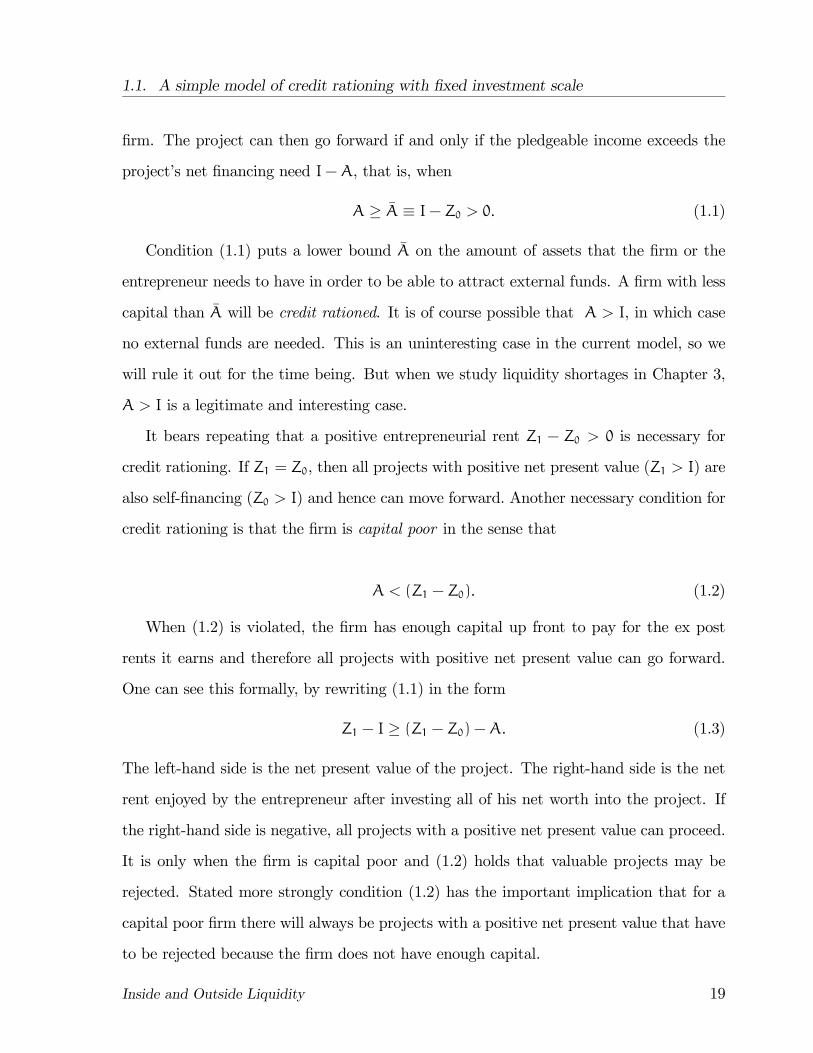
entrepreneur with an investment opportunity that is worth Z1 to him, but only Z0 < Z1
to outside investors. We assume that the initial investment I satisfies Z1 > I > Z0 (see
Figure 1.1). The investment has a positive Net Present Value, Z1 > I, but it is not self-
financing, because the most that investors can be promised is less than the investment
Z0 < I. The shortfall I− Z0 > 0 must be paid by the entrepreneur (or covered by claims
on the market value of the firm’s other existing assets).
One can give a variety of reasons why the full returns of a project cannot be paid out
to the investors, that is, why there is a positive wedge (entrepreneurial rent) Z1 −Z0 > 0.
They can be put into two general categories: explanations based on exogenous constraints
on payouts and those based on endogenous constraints. The prime example of exogenous
Inside and Outside Liquidity 17
1.1. A simple model of credit rationing with fixed investment scale
constraints are private benefits that only the entrepreneur can enjoy, such as the pleasure
of working on a favorite project or the increased social status that comes with its success.
A related intangible benefit arises from differences in beliefs. Entrepreneurs often have
an inflated view of the chances that their project will succeed.1 To the extent that such
differences in beliefs are not based on better information, the extra utility the entrepreneur
derives from overoptimism can in a one-shot setting be modeled as a private benefit that
investors do not value. There are also tangible benefits that may be impossible to transfer
fully, such as the increased value of human capital that comes with investment experience,
or the future value that an entrepreneur may enjoy from the option to move after he has
been revealed to be a good performer. 2
In the second category, entrepreneurial rents emerge endogenously, because even though
it is feasible to pay out all of the project’s returns to the investors, attempts to reduce the
entrepreneur’s share below Z1 −Z0 > 0, will inevitably hurt the investors as well. There-
fore it is optimal to let the entrepreneur enjoy a minimum rent. The simplest example
is one where the entrepreneur can steal some of the output for private consumption or,
equivalently, one where the entrepreneur has to be given a share of the output in order
to discourage him from diverting output to private consumption (Lacker and Weinberg,
1989). Below, we will consider a standard moral hazard model with limited liability that
leads to the same conclusion.
Because we assumed that the project is not self-financing, I−Z0 > 0, investment will
require a positive contribution from the entrepreneur. Let A be the maximum amount of
capital that the entrepreneur can commit to the project either personally or through the
1Of course the fact that entrepreneurs often fail or that they express a high confidence in a project
when asked, are as such no evidence of overconfidence and can be explained by either agency costs or
confidence-maintenance strategies. However, Landier and Thesmar (2009) provide evidence of entrepre-
neurial overconfidence, which is consistent with Van den Steen (2004). Simsek (2010) analyzes financing
of projects sponsored by optimistic entrepreneurs. He shows that heterogeneity in beliefs has a very
asymmetric impact on financing, as financial market discipline operates only when entrepreneurial op-
timism concerns the likelihood of bad events. Entrepreneurs who are optimistic about good events can
raise substantial amounts by contrast.2See, e.g., Terviö (2009).
Inside and Outside Liquidity 18
1.1. A simple model of credit rationing with fixed investment scale
firm. The project can then go forward if and only if the pledgeable income exceeds the
project’s net financing need I−A, that is, when
A ≥ A ≡ I− Z0 > 0. (1.1)
Condition (1.1) puts a lower bound A on the amount of assets that the firm or the
entrepreneur needs to have in order to be able to attract external funds. A firm with less
capital than A will be credit rationed. It is of course possible that A > I, in which case
no external funds are needed. This is an uninteresting case in the current model, so we
will rule it out for the time being. But when we study liquidity shortages in Chapter 3,
A > I is a legitimate and interesting case.
It bears repeating that a positive entrepreneurial rent Z1 − Z0 > 0 is necessary for
credit rationing. If Z1 = Z0, then all projects with positive net present value (Z1 > I) are
also self-financing (Z0 > I) and hence can move forward. Another necessary condition for
credit rationing is that the firm is capital poor in the sense that
A < (Z1 − Z0). (1.2)
When (1.2) is violated, the firm has enough capital up front to pay for the ex post
rents it earns and therefore all projects with positive net present value can go forward.
One can see this formally, by rewriting (1.1) in the form
Z1 − I ≥ (Z1 − Z0)−A. (1.3)
The left-hand side is the net present value of the project. The right-hand side is the net
rent enjoyed by the entrepreneur after investing all of his net worth into the project. If
the right-hand side is negative, all projects with a positive net present value can proceed.
It is only when the firm is capital poor and (1.2) holds that valuable projects may be
rejected. Stated more strongly condition (1.2) has the important implication that for a
capital poor firm there will always be projects with a positive net present value that have
to be rejected because the firm does not have enough capital.
Inside and Outside Liquidity 19

1.2. A simple moral hazard model illustrating the wedge
between value and pledgeable income
Let us finally note that the internal cost of capital is above the market rate (0) below
the point where the firm is credit rationed as can be seen by considering the entrepreneur’s
utility payoff U.
U = A+ Z1 − I, if A ≥ A,
U = A, if A < A.
(1.4)
Because utility jumps up atA = A, the value of funds inside the firm is strictly higher than
outside the firm below A.3 When A < A total output can be increased by transferring
funds from investors to capital poor entrepreneurs, but of course such transfers will not
be Pareto improving. In models with non-transferable utility, Pareto optimality does not
imply total surplus maximization.
1.2 A simple moral hazardmodel illustrating the wedge
between value and pledgeable income
The wedge as an incentive payment
Our liquidity analysis proceeds largely without reference to the particular reasons
behind the non-pledgeable income wedge Z1 − Z0. But to gain a better grasp of the
economic significance of this analysis, it is worth going beyond the reduced-form model.
In this section, we will analyze in detail a specific model in which the wedge appears
endogenously.4 The analysis will highlight important determinants of the firm’s debt
capacity, illustrate the impact that credit rationing may have on the firm’s choice of
investments and indicate the benefits and costs of using different kinds of collateral.
We employ a standard model of investment with moral hazard.5. There is a single
3Formally, the marginal internal cost of capital is equal to 0 up to A and jumps to infinity at A. With
a continuous investment choice this cost varies more smoothly and exceeds the market rate: See section
1.3.4We should stress that even if a number of explanations can be given for a positive wedge, it is of
course not true that we can always take the wedge as a primitive in our analysis. This is one reason
to provide an explicit model that justifies treating the wedge as exogenous in the analyses we will be
considering.5The model is taken from Holmström and Tirole (1998), but has many antecedents.
Inside and Outside Liquidity 20
1.2. A simple moral hazard model illustrating the wedge
between value and pledgeable income
entrepreneur (firm) and a competitive set of outside investors. All parties are risk neutral.
There is a single good used for consumption as well as investment. There are two periods.
In the initial period, indexed t = 0, there is an opportunity to invest. The investment
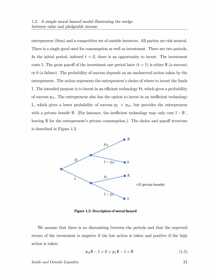
costs I. The gross payoff of the investment one period later (t = 1) is either R (a success)
or 0 (a failure). The probability of success depends on an unobserved action taken by the
entrepreneur. The action represents the entrepreneur’s choice of where to invest the funds
I. The intended purpose is to invest in an efficient technology H, which gives a probability
of success pH. The entrepreneur also has the option to invest in an inefficient technology
L, which gives a lower probability of success pL < pH, but provides the entrepreneur
with a private benefit B. (For instance, the inefficient technology may only cost I − B ,
leaving B for the entrepreneur’s private consumption.). The choice and payoff structure
is described in Figure 1.2.
We assume that there is no discounting between the periods and that the expected
return of the investment is negative if the low action is taken and positive if the high
action is taken:
pHR− I > 0 > pLR− I+ B (1.5)
Inside and Outside Liquidity 21
1.2. A simple moral hazard model illustrating the wedge
between value and pledgeable income
Thus, it is better not to invest at all than to invest and have the firm choose the inefficient
technology L.
The entrepreneur has assets worth A. These assets are liquid in the sense that they
have the same value in the hands of the entrepreneur as in the hands of investors. The
firm is protected by limited liability. We assume again that A < I so that the firm needs
to raise I−A > 0 from outside investors in order for the project to go forward. Investors
can access an unlimited pool of funds and demand an interest rate that we normalize to
0.
Investors can be paid contingent on the outcome of the project. Let Xs (Xf) be the
entrepreneur’s date-1 wealth in case the project succeeds (fails). Limited liability requires
that Xi ≥ 0, i = s, f. Investors receive Ys = R−Xs if the project succeeds and Yf = −Xf
if it fails.
We are interested in the conditions under which the investment can go ahead. There
are two constraints that must be satisfied. First, the investors need to break even,
pH(R− Xs) + (1− pH)(−Xf) ≥ I−A. (1.6)
Second, the entrepreneur must be induced to be diligent,
pHXs + (1− pH)Xf ≥ pLXs + (1− pL)Xf + B (1.7)
Simplified, this incentive compatibility constraint reads
Xs − Xf ≥ B
∆p, (1.8)
where
∆p ≡ pH − pL > 0. (1.9)
Incentive compatibility (1.8) paired with limited liability implies that the entrepreneur
earns a positive rent. This rent is minimized by setting Xf = 0 and Xs =B∆p. The rent
cuts into the amount that can be paid out to investors. The firm’s pledgeable income
Inside and Outside Liquidity 22
1.2. A simple moral hazard model illustrating the wedge
between value and pledgeable income
is defined as the maximum expected amount that investors can be promised when the
entrepreneur is paid the minimum rent. The pledgeable income is
Z0 = pH(R−B
∆p). (1.10)
To complete the link to the reduced form discussed earlier, denote the total pie Z1 = pHR.
The positive wedge is then equal to the entrepreneur’s minimum rent Z1 − Z0 = pHB∆p.
Factors influencing pledgeable income
(a) Bias towards less risky projects. The net worth of a firm may prohibit it from
investing altogether as discussed above. More generally, a firm’s net worth will merely
limit which projects it can invest in. Assume there is a set of projects that the firm and
the investors can jointly choose from. The firm can more easily satisfy (1.1) by reducing
the investment scale I or by choosing projects with a higher pledgeable income.
For example, in the incentive-payment illustration, each project is characterized by a
tuple (I, R, pH, pL, B), where we allow the inefficient project to vary with the efficient one
(the entrepreneur’s alternative use of funds may depend on the project to be undertaken).
Pledgeable income increases in pH and R and decreases in pL and B, reflecting the fact
that the entrepreneur’s incentive problem is less severe when the efficient project becomes
more attractive relative to the inefficient one. More interestingly, consider variations in
pH and R that leave the expected payoff of the desired project Z1and the other parameters
unaltered. Specifically, assume that pH goes down while R goes up so that the project
becomes more risky. Other things equal, the firm’s pledgeable income decreases with such
risk. A decrease in pH increases the rentpHB
∆pthat goes to the entrepreneur, because the
entrepreneur’s reward in the successful state (the only incentive instrument available) is
less potent the lower is pH. With a higher entrepreneurial rent, less can be promised to
investors (Z0 is lower), which raises the cut-off value A. At the margin, therefore, capital-
constrained firms will accept safer projects at the expense of lower expected returns.
(b) Diversification. As a variant on this theme, one can ask whether diversification
Inside and Outside Liquidity 23
1.2. A simple moral hazard model illustrating the wedge
between value and pledgeable income
will help to reduce the need for own funds. Suppose a single project can be replaced by
two identical, half-sized projects of the sort we have discussed. Further, assume that the
projects are stochastically independent and that the entrepreneur chooses separately but
simultaneously whether to be diligent in each project. One can show that in this case
the optimal incentive scheme pays the entrepreneur a positive amount only when both
projects succeed. In effect, the entrepreneur pledges the rewards that would accrue from
a successful project as collateral for the other project (and conversely). This maximizes
the pledgeable income.
For diversification to be of value, it is important that the projects be independent. If
the projects were perfectly correlated (or the entrepreneur opportunistically chose them
to be perfectly correlated), diversification would not raise the pledgeable income.6
(c) Intermediation. Another way of increasing the pledgeable income is to reduce the
entrepreneur’s opportunity cost of being diligent. Some projects are more conducive to
misbehavior than others: for instance, those that are exceptional, that do not have tan-
gible investments, or that involve poor accounting. A capital poor firm can sometimes
increase its pledgeable income by turning to an intermediary that has monitoring exper-
tise. A simple way to model monitoring is to assume that the intermediary can reduce
B to a lower level b (and perhaps simultaneously reduce pL), because it can place con-
straints on what the firm can do. Loan covenants serve this purpose: for instance, lending
contracts frequently forbid the firm from paying dividends if certain financial conditions
are violated. Covenants may also give the bank veto rights on the sale of strategic assets
and spell out circumstances under which the bank can intervene even more aggressively
by getting the right to nominate all or part of the board. Another potential interpre-
tation of the monitoring activity is that the bank acquires information that is relevant
for decision-making and uses it to convince the board not to rubberstamp (what turns
6For more on diversification in this type of model, see Conning (2004), Hellwig (2000), Laux (2001)
and Tirole (2006, chapter 4).
Inside and Outside Liquidity 24
1.2. A simple moral hazard model illustrating the wedge
between value and pledgeable income
out to be) the management’s pet project. In the model, and apparently in reality, giving
the firm less attractive outside options reduces entrepreneurial rents, increases pledgeable
income and thus lowers A. The carrot can be smaller if the stick is stronger.
Of course, intermediation is not free, and in order to determine whether intermediaries
can really increase pledgeable income, one has to consider monitoring costs, which will
move A back up. One can distinguish at least three kinds of monitoring costs from
intermediation:
• First, direct costs are incurred by the intermediary as well as the firm due to the
additional work involved in evaluating investments, processing loans and monitoring
compliance with covenants.
• Second, the constraints imposed on a firm as part of a loan covenant do not merelycut out illegitimate opportunities; they also cut out legitimate ones. A firm that
cannot sell or acquire significant assets without the approval of a bank may have
to forego valuable deals. Excluding profit opportunities of this kind lowers Z1 and
reduces the project’s expected return.
• Third, monitoring expertise is scarce and commands rents that depend on marketconditions. In Holmström and Tirole (1997), we study a model where the monitor
can itself act opportunistically and therefore has to be given a share in the firm’s
payoff. This increases A by an amount that gets determined by the demand for
intermediation among credit-constrained firms. In equilibrium firms sort themselves
into three groups as a function of their net worth: (i) those firms that have too little
own capital to be able to invest; (ii) those that have enough own capital that they
can go directly to the market and do not need intermediation; and (iii) those that
have intermediate amounts of capital and invest with the help of intermediaries. In
the last instance, funding comes both from informed investors (intermediaries) and
from the uninformed investors (the general market), who invest only because the
Inside and Outside Liquidity 25
1.3. Variable investment scale
intermediary’s participation has reduced the risk of opportunism.
1.3 Variable investment scale
For the upcoming liquidity analysis we need a model where the scale of investment is
variable, so that we can study the important trade-off between the scale of the initial
investment and the decision to save some funds to meet future liquidity shocks. A simple,
tractable model is obtained by letting the investment vary in a constant-returns-to-scale
fashion.
Let I be the scale of the investment (measured by cost), let ρ1 be the expected total
return, and ρ0 the pledgeable income, both measured per unit invested. Thus, I results in
a total payoff ρ1I of which ρ0I can be pledged to outside investors. The residual (ρ1−ρ0)I
is the minimum rent going to the entrepreneur.
The moral-hazard example of section 1.2 fits this framework if we assume that a
successful project returns RI and the private benefit to the entrepreneur from cheating is
BI. In that case,ρ1 = pHR,
ρ0 = pH(R− B∆p).
(1.11)
As before, we assume that projects are socially valuable, but not self-financing:
0 < ρ0 < 1 < ρ1. (1.12)
Consequently, the entrepreneur needs own funds A > 0 to invest. For each unit of
investment, the firm can raise ρ0 from outside investors, leaving the minimum equity ratio
1− ρ0 > 0 to be covered by own funds. The repayment constraint is
A ≥ (1− ρ0)I,
implying a maximum investment scale
I = kA =A
1− ρ0. (1.13)
Inside and Outside Liquidity 26
1.3. Variable investment scale
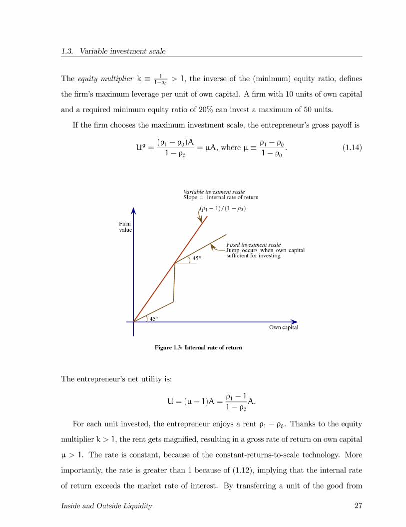
The equity multiplier k ≡ 11−ρ0
> 1, the inverse of the (minimum) equity ratio, defines
the firm’s maximum leverage per unit of own capital. A firm with 10 units of own capital
and a required minimum equity ratio of 20% can invest a maximum of 50 units.
If the firm chooses the maximum investment scale, the entrepreneur’s gross payoff is
Ug =(ρ1 − ρ0)A
1− ρ0= μA, where μ ≡ ρ1 − ρ0
1− ρ0. (1.14)
The entrepreneur’s net utility is:
U = (μ− 1)A =ρ1 − 1
1− ρ0A.
For each unit invested, the entrepreneur enjoys a rent ρ1 − ρ0. Thanks to the equity
multiplier k > 1, the rent gets magnified, resulting in a gross rate of return on own capital
μ > 1. The rate is constant, because of the constant-returns-to-scale technology. More
importantly, the rate is greater than 1 because of (1.12), implying that the internal rate
of return exceeds the market rate of interest. By transferring a unit of the good from
Inside and Outside Liquidity 27
1.3. Variable investment scale
investors to the entrepreneur, total social surplus (ρ1I − I) could be increased by more
than one unit. But such transfers are not Pareto improving, since the increase in total
surplus cannot be arbitrarily split between the investors and entrepreneurs. In models
with limited liability, total surplus maximization is not a necessary condition for Pareto
optimality.
Because the rate of return on entrepreneurial capital exceeds the market rate, it is
evident that the entrepreneur maximizes his utility by choosing the maximum investment
scale (1.14). He puts all his wealth in the illiquid portion of the return (the non-pledgeable
return (ρ1 − ρ0)I ), leaving outsiders holding the firm’s liquid assets. Again, total output
could be raised by transferring wealth from passive investors to active entrepreneurs, but
since investors could not be compensated as they already hold all the firm’s liquid claims,
this would not be Pareto improving. There is nothing that the government could do to
improve on private contracting.
Comparative statics and investment implications
Factors that increase ρ0 or ρ1 (or both) will increase the entrepreneur’s utility and an
increase in ρ0 will also increase the investment scale I. Recall that in the moral-hazard
model, ρ0 increases with R and pH and decreases with B and pL, while ρ1 increases with R
and pH. Investors are simply paid their market rate of return, so they remain unaffected
by these changes.
If the firm could choose among investments that differed in their attributes ρ0 and ρ1,
the firm would not want to choose the investment that maximizes the social net present
value, that is, the investment with the highest ρ1. The pledgeable income is also critical
as it determines the extent to which the firm can lever its capital. From (1.14) we see
that the firm’s willingness to substitute ρ0 for ρ1 is given by
dρ1dρ0
= 1− μ < 0. (1.15)
The firm will choose projects with lower ρ1 up to the point where the reduction in ρ1 per
Inside and Outside Liquidity 28

1.3. Variable investment scale
unit of increase in ρ0 equals the difference between the internal rate of return and the
market rate of return. Each unit of pledgeable income ρ0 is worth μ units of ρ1, because
of scale expansion. This illustrates one of the central themes of credit constrained lending:
the willingness to sacrifice net present value for an increase in pledgeable income.
Inside and Outside Liquidity 29
Chapter 2
A simple model of liquidity demand
Firms demand liquidity in anticipation of future financing needs either because it is
cheaper to get financing now or because there is a risk that financing will not be available
if the firm waits until the need for funding arises. In this chapter we will analyze the
demand for liquidity in a simple extension of the two-period model from section 1.3. The
basic idea is easy to understand. Suppose there is an intermediate period when additional
funds have to be invested in order to continue the project and realize any payoffs. We refer
to this reinvestment need as a liquidity shock and denote it ρ (per unit of investment).
If the liquidity shock ρ turns out to be larger than the pledgeable amount ρ0, the firm
cannot get outside funding to continue the project unless it has arranged for such funding
in advance. This creates a demand for liquidity, as firms look to insure against shocks
that have a high total return (ρ1 − ρ > 0), but a negative net present value for investors
(ρ0 − ρ < 0). Note that the wedge ρ1 − ρ0 > 0 is crucial for the argument. If ρ1 = ρ0,
the liquidity shock ρ cannot fall strictly between the total and the pledgeable return.
The ex ante demand for liquidity will depend on the size of the liquidity shock. Shocks
that are high enough will not be insured (financed in advance). The second best policy
trades off the scale of the initial investment against the ability to withstand higher liquidity
shocks. In general, there will be credit rationing both at the initial period and in the
intermediate period, because entrepreneurial capital is scarce and commands a premium
relative to the market.
30

2.1. The general set up
By definition no external claims can be issued on the private (illiquid) return ρ1 − ρ0,
while arbitrary external claims can be issued on the pledgeable (liquid) return ρ0. In
particular, these claims can be made contingent on the liquidity shock ρ. In effect, we are
assuming complete contracting on the liquid portion of the firm’s return. This is perhaps
unrealistic, but it has the attraction that it is a minimal departure from the standard
Arrow-Debreu world. We will discuss how second-best contracts can be implemented
using common ways such as credit lines, equity issues (involving dilution) or by holding
liquid (marketable) assets in anticipation of future liquidity needs. Finally, and relaxing
the assumption that the liquidity shock is observed by investors, we will also show that
the implementation of the second-best policy hinges crucially on the ability of investors
to keep the firm from spending funds on unauthorized projects.
2.1 The general set up
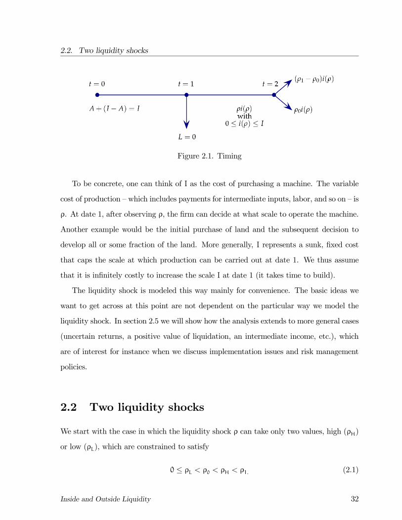
There are three dates t = 0, 1, 2 and a single good. At date 0 the firm chooses the scale
of the project I. At date 1 the liquidity shock ρ ≥ 0 takes place. The value ρ determineshow much more needs to be invested per unit to continue. Continuing at a smaller scale
than I is feasible. Let i(ρ) ≤ I denote the continuation scale when the liquidity shockis ρ. Continuing at this scale requires a date-1 investment ρi(ρ) and yields a date-2
public (pledgeable) return ρ0i(ρ) and an illiquid (private) return (ρ1 − ρ0)i(ρ) to the
entrepreneur. There are no returns from the portion of the project that is not carried
forward. If i(ρ) = 0 the firm is closed down and the payout, both pledgeable and private,
is zero.
Inside and Outside Liquidity 31
2.2. Two liquidity shocks
Figure 2.1. Timing
To be concrete, one can think of I as the cost of purchasing a machine. The variable
cost of production — which includes payments for intermediate inputs, labor, and so on — is
ρ. At date 1, after observing ρ, the firm can decide at what scale to operate the machine.
Another example would be the initial purchase of land and the subsequent decision to
develop all or some fraction of the land. More generally, I represents a sunk, fixed cost
that caps the scale at which production can be carried out at date 1. We thus assume
that it is infinitely costly to increase the scale I at date 1 (it takes time to build).
The liquidity shock is modeled this way mainly for convenience. The basic ideas we
want to get across at this point are not dependent on the particular way we model the
liquidity shock. In section 2.5 we will show how the analysis extends to more general cases
(uncertain returns, a positive value of liquidation, an intermediate income, etc.), which
are of interest for instance when we discuss implementation issues and risk management
policies.
2.2 Two liquidity shocks
We start with the case in which the liquidity shock ρ can take only two values, high (ρH)
or low (ρL), which are constrained to satisfy
0 ≤ ρL < ρ0 < ρH < ρ1. (2.1)
Inside and Outside Liquidity 32
2.2. Two liquidity shocks
The reason for limiting the shocks in this manner is that shocks below ρ0 do not require
pre-arranged financing, while shocks above ρ0 do. The high and low shocks in (2.1) cover
these two leading cases. Let fL and fH denote the probabilities of a low, respectively high
liquidity shock. We assume that
ρ0 < min1+ fLρL + fHρH,1+ ρLfL
fL < ρ1. (2.2)
The middle term in (2.2) is the minimum expected cost of carrying one unit of the
project to completion (see below). If the project is continued in both states the expected
cost is the first term in the brackets. If the project is continued only in the low state,
the second term measures the expected cost per unit completed. The inequality on the
right implies that the project is socially desirable, while the inequality on the left assures
that the project is not self-financing (the pledgeable income does not cover the total cost
of investment regardless of the optimal policy). A self-financing project could be carried
out at any scale, which would lead to unbounded payoffs.
We are looking for a second-best contract. A contract specifies the level of investment
I and the continuation scales iL ≡ i(ρL) and iH ≡ i(ρH) (both ≤ I) corresponding to thelow and high liquidity shocks, respectively. A contract also specifies final payments to
investors and the entrepreneur, but just as in the simpler two-period model it is easy to
see that it is optimal to assign all the liquid returns ρ0i(ρ) to the investors, leaving the
entrepreneur holding only the illiquid part (ρ1 − ρ0)i(ρ). The entrepreneur only holds
illiquid claims because the return on internal liquid funds exceeds the market rate (which
we take to be 0).
The second-best solution solves:
max I,iL ,iH fL(ρ1 − ρL)iL + fH(ρ1 − ρH)iH − I ,
subject to
(2.3)
fL(ρ0 − ρL)iL + fH(ρ0 − ρH)iH ≥ I−A, (2.4)
Inside and Outside Liquidity 33
2.2. Two liquidity shocks
0 ≤ iL, iH ≤ I (2.5)
The objective function is the expected social return of the investment. Evidently, the
budget constraint (2.4) will bind at the optimum. By substituting the budget constraint
into the objective function, eliminating I, we get an equivalent program in which the
entrepreneur’s expected rent rather than the expected social return is maximized. Since
investors all earn the market rate of interest (0), the full social surplus goes to the entre-
preneur. We will often take the entrepreneur’s rent, which equals his expected net utility,
as the objective.
The budget constraint makes clear that investors provide insurance against liquidity
shocks. When the low shock occurs, the firm pays the investors ρ0 − ρL > 0. When the
high shock occurs, investors pay the firm ρH − ρ0 > 0 per unit of continued investment.
Since ρ1 − ρL and ρ0 − ρL are both positive, it is in the interest of the investors as
well as the entrepreneur to continue at full scale when a low shock occurs; hence iL = I.1
The program then boils down to choosing just two values: the initial scale I and the
continuation scale iH in the high shock state. There is a trade-off between these two
investments. The bigger one chooses I the lower must iH be, since both imply net outlays
for the investors (in contrast to iL, which relaxes the budget constraint). Let x = iH/I
denote the fraction of the project that is being continued at date 1 and let
ρ(x) ≡ fLρL + fHρHx (2.6)
denote the expected unit cost of continuing. The maximal scale of the initial investment
I(x) as a function of the fraction x of the project that is continued in the high shock state
1Because the project always continues at full scale when the low shock occurs, we could have counted
the low shock as part of the initial investment and adjusted both the low and the high shock corre-
spondingly; that is, we could have chosen ρL = 0 without loss of generality. When there is a positive
liquidity premium, as will be the case later on, the same nominal expenditure may have a different value
in different periods; hence we refrain from this simplification.
Inside and Outside Liquidity 34
2.2. Two liquidity shocks
is given by the budget constraint (2.4):
I(x) =A
1+ ρ(x)− ρ0(fL + xfH)(2.7)
The entrepreneur’s expected net utility (equal to the social surplus) is
U(x) = [ρ1(fL + fHx)− (1+ ρ(x))]I(x) (2.8)
= μ(x)A,
where μ(x) is the net value of an additional unit of entrepreneurial capital and takes the
form
μ(x) =ρ1(fL + fHx)− (1+ ρ(x))
(1+ ρ(x))− ρ0(fL + fHx). (2.9)
Because the Lagrangian of the program (2.3)-(2.5) is linear, we only need to evaluate
the utility levels corresponding to x = 0 (continuing only when the shock is low) and x = 1
(always continuing). In either case continuation is at full scale I; partial continuation is
not relevant. A direct evaluation of U(1)−U(0), the difference in utility between the two
cases, shows that it is optimal to cover both liquidity shocks (choose x = 1) if and only if
ρ1fL − (1+ ρLfL)
(1+ ρLfL)− ρ0fL= μ(0) ≤ μ(1) =
ρ1 − (1+ ρ(1))
(1+ ρ(1))− ρ0. (2.10)
When ρH = ρL, inequality (2.10) holds and the project will be continued in both
states. As ρH is increased from ρL to ρ1, the difference μ(0)− μ(1) moves monotonically
from being strictly negative to strictly positive. Therefore, in between the two extreme
ρH-values there is a cut-off value c, satisfying ρL < c < ρ1, such that the project will
continue if and only if
ρH ≤ c. (2.11)
Simple manipulations of the cut-off condition μ(0) ≤ μ(1) allow us to write
c = min
¯1+ fLρL + fHρH,
1+ fLρLfL
°. (2.12)
Inside and Outside Liquidity 35
2.2. Two liquidity shocks
We can interpret c as the unit cost of effective investment, i.e. what it costs on average to
bring one unit of investment to completion. Condition (2.11) therefore has the intuitive
interpretation that it is optimal to continue in the high-shock state if and only if the
unit cost of effective investment is less than the cost of the shock. We will see that an
analogous condition holds in the continuum case.
We can also restate the inequality (2.10) as the following necessary and sufficient
condition for continuing in both the low and the high state2
fL(ρH − ρL) ≤ 1. (2.13)
The effects of ρH and ρL in (2.13) are intuitive. They reflect the fact that both an increase
in ρH and a decrease in ρL will work in favor of larger ex-ante scale at the expense of less
ex-post liquidity; a lower ρL increases the return to initial scale, while a higher ρH makes
it more costly to continue ex post. The role played by fL in (2.13) is less obvious, since
both the benefits and costs of continuing in the high state go up as fL decreases. The
issue then is how the firm should divide an extra unit between the initial investment I
and liquidity provision at date 1. As fL goes to zero, the net return from investing only
in the low-shock state goes to zero, while the net return from continuing in both states is
bounded below by a strictly positive number. Hence, if fL is small enough it is better to
continue also in the high state.
Remark (repeated liquidity shocks). A limitation of our analysis is that it does not do
justice to the rich dynamics of liquidity management. Indeed, after the initial contracting
stage, date 0, there is only one period, date 1, at which the firm will possibly need new
cash. There is accordingly no point hoarding liquidity at date 1. Relatedly, all liquidity
hoarded at date 0 is usable,3 with the caveat, studied in Appendix 2.1, that available
liquidity may be abused in the presence of alternative uses of this liquidity. Recent
2That neither ρ0 or ρ1 show up in (2.13) is a consequence of the constant returns to scale technology;
however, they enter implicitly through the parameter restrictions (2.1) and (2.2).3See Goodhart (2008) for a discussion of usable liquidity.
Inside and Outside Liquidity 36
2.3. Implementation of the second best contract
work has studied optimal liquidity management in related, but infinite-horizon models of
repeated moral hazard. Biais et al. (2007, 2008) and DeMarzo and Fishman (2007 a,b)
shed light on how over time investment and available liquidity adjust to profit realizations
in an optimal contract. For example Biais et al. show that liquidity is not meant to be
fully depleted even though it is indeed reduced after an adverse shock. Discipline is
ensured by downsizing when things go wrong, not by a complete exposure to liquidity
risk. This policy is in the spirit of proportionality for compulsory reserves as well as for
capital requirements in banking regulation.
2.3 Implementation of the second best contract
Implementation of the second-best contract presents two kinds of problems. The first
problem is that the entrepreneur may use the funds in a different way than the contract
specifies (either at date 0 or at date 1). The second problem is that investors may not be
able to deliver on the promise to provide funds at date 1. Such promises must be backed
up by claims on real assets that the investor owns at date 1 and can use as collateral.
We will discuss collateral problems at length in the coming chapters. The purpose of this
section is to illustrate some of the problems that may arise on the firm’s side.
One potential problem is that, when the second best optimum specifies that the firm
should not continue when facing the high shock, the entrepreneur may nonetheless want
to invest less than the agreed-upon amount I at date 0 in order to keep extra funds in
store to meet the high liquidity shock. Alternatively, when the second best optimum
recommends to withstand even the high liquidity shock, the entrepreneur may not want
to save funds for reinvestment in the high state and instead spend the funds on a higher
initial investment I. This can be a tempting possibility, since the entrepreneur knows that
investors will always finance a low shock, even if the scale is higher than initially intended.
The entrepreneur can rely on a soft-budget constraint for the low shock, because investors
face a fait accompli. The downside to the entrepreneur of such a policy is that there will
Inside and Outside Liquidity 37
2.3. Implementation of the second best contract
not be enough funds to finance the high shock, and no investor will be ready to make up
the short-fall at date 1.
In order to implement the second-best policy, there must be a way to enforce the
right levels and kinds of investment at date 0 as well as date 1. Intermediaries, venture
capitalists, large block holders and others monitor in varying degrees and in different ways
a firm’s use of funds. A rich literature in corporate finance has investigated these issues in
depth. We will not study intermediation explicitly, even though it constitutes an integral
part of the financing of firms.4 Instead, we will assume that investors can directly monitor
the firm’s liquidity position but not the firm’s liquidity shock and consider two illustrative
cases: in the first, the firm has no alternative uses of funds and will therefore behave; in
the second case, the entrepreneur can divert funds for some personal benefit.
Costless implementation: firm has no alternative use of funds
Assume condition (2.10) holds so that reinvestment is desirable both in the low and the
high shock state. Consider first the rather hypothetical scenario in which the entrepreneur
has no alternative use of date-1 funds; date-1 liquidity is of value only because it allows
the firm to meet liquidity shocks. Under this scenario, there are many alternative ways
to implement the second-best solution.
One option is to give the firm a line of credit up to ρHI, which it can freely use at date
1. This allows the firm to meet both kinds of shocks. If the low shock occurs, the firm will
leave (ρH − ρL)I unspent, since we assumed that there is no alternative use for the excess
funds. If the high shock occurs, the firm will draw down the full line of credit, which has
a negative net present value, because the firm’s pledgeable date-2 income ρ0I is less than
the credit ρHI used. A minor variant would be to reduce the credit line to (ρH − ρ0)I
and giving the entrepreneur the right to dilute the initial investors’ up to their maximum
stake ρ0I. Either way, the entrepreneur has to pay for the expected use of liquidity up
4See Holmström and Tirole (1997) for an analysis of intermediation using the same basic model as
here and Tirole (2006) for a more extensive treatment.
Inside and Outside Liquidity 38
2.3. Implementation of the second best contract
front.
One may wonder to what extent banks actually honor credit lines in states of nature
where they would prefer not to lend. Empirically, it is not an easy question to distinguish
involuntary lending from voluntary lending or lending that is done to preserve a reputation
in the credit market as has been suggested by Boot, Thakor and Udell (1987).5 However,
studies of bank lending during the subprime crisis as well as the 1998 crisis associated
with the collapse of Long Term Capital Management, indicate that drawdowns on existing
credit lines can be substantial. Ivanisha and Scharfstein (2009), who compared patterns
of bank lending in the period August-November 2008 note that while new commercial and
industrial loans fall dramatically (37%) in this period compared with the same period in
2007, firms that secured credit lines likely made extensive use of them, since the level
of loans on bank balance sheets increased somewhat during that time. They identify
$16 billion worth of drawdowns from press releases alone, but considering the large stock
of credit lines (about $3,500 billion) the total drawdowns must be much larger. The
paper further documents that banks that were liquidity constrained had to reduce their
other lending in order to handle drawdowns — an opportunity cost argument that points
to the involuntary nature of honoring credit lines. Anecdotal evidence indicates that
a large number of firms also drew down credit lines in anticipation of future liquidity
problems caused by the crisis, suggesting that firms have been concerned about either
the credit worthiness of banks or changes in the terms of the credit facility. Strahan,
Gater and Schuermann’s (2006) study of the LTCM crisis likewise concludes that banks
and other credit institutions had to accept costly drawdowns, though the overall effect on
the banking system was moderated by the fact that the funds came back in the form of
deposits. On balance, the evidence indicates that credit lines do serve an insurance role
5Banks’ implicit liabilities are common and create serious issues for prudential regulators as they are
not really covered by any capital charge. For example, in the summer of 2007, Bear Stearns bailed out
two funds it had sponsored even though it had no legal obligation to do so.
Inside and Outside Liquidity 39
2.3. Implementation of the second best contract
of the sort envisioned in our model.6
Another common arrangement to guarantee that the firm will have enough resources
in adverse circumstances is for the firm to buy protection. Credit default swaps (CDSs),
which amounted to $62 trillions at the onset of the recent crisis, allow firms to buy
protection against the default of other firms.7 For example, if an amount exceeding
(ρH − ρ0)I constitutes a shortfall of income due to the default of trading partners, the
shortfall can be offset through the use of CDSs.
Finally, firms routinely hoard liquid funds, sometimes very large ones, both to cush-
ion smaller liquidity shocks as well as in anticipation of future spending needs such as
acquisitions and other kinds of investments.8. This can be represented in our model by
investors paying the firm I + (ρH − ρ0)I −A at date 0 and making sure the firm hoards
liquid assets, for instance treasury bonds, at date 0 in the amount (ρH − ρ0)I. At date
1, the firm can raise up to ρHI in fresh funds by selling the bonds and by diluting the
stake of the initial investors through additional equity. If the liquidity shock is low, the
firm simply leaves the excess liquidity unused — does not issue new equity and/or does
not use all of the bonds. Note that this way of implementing the second-best outcome,
while equivalent to a credit line, does not require the firm to raise fresh funds at date
1 for a project that has a negative net present value. The funds covering negative net
present value actions at date 1 have been paid already at date 0. Naturally, one can mix
hoarding with credit lines in a lot of ways as long as the firm can access the right amount
6Credit lines are often contingent on satisfying loan covenants, which could be interpreted as an
effort to deal with states where firms, even in the second-best, should not be extended credit. In the
recent crisis and especially in the final years before the collapse, many banks appear to have abandoned
usual precautions and extended “covenant-light” credit lines, tempted by the generous up-front fees for
contingent credit.7The $62 trillions figure is the gross value of CDSs and greatly overstates the actual insurance coverage
for this reason. Also, many participated in these markets for reasons other than insuring themselves. The
CDS market was in part a place where bets could be placed on the future of the economy.8For instance, Microsoft had at one point over $40 billion in liquid assets. Very little is typically
invested in the stock of other companies, unless there is some strategic purpose to do so or the firm is
in the investment business as such. Our focus is on liquidity shocks, but as the analysis in section 2.5
shows, we could include other motives. However, given our “complete market” assumption, we cannot
explain the heavy use of debt and near-debt assets.
Inside and Outside Liquidity 40
2.3. Implementation of the second best contract
of liquidity at date 1.
Costly implementation: firm can divert funds at date 1
The assumption that the firm has no alternative use for excess liquidity is extreme.
Firms always have alternative investments to consider, especially if the funds come at
no extra charge as above. In Appendix 2.1 we illustrate with a simple example how the
optimal contract responds to the presence of an alternative investment option.
Consider again the two-shock model in which (2.10) holds, so that the second-best
contract prescribes continuation for both the low (ρL) and the high (ρH) liquidity shock.
Suppose that the firm can divert funds at date 1 to a project that only generates private
benefits. Each unit diverted into the alternative project generates a benefit to the entre-
preneur that is equal to ξ units of consumption. We assume that the value of a diverted
unit satisfies
ξ ≤ 1, (2.14)
so that it is more efficient for the entrepreneur to receive one unit from the pledgeable
income at date 2 than to divert one unit at date 1.
Investors can observe howmuch funds the firm uses in total at date 1 as well as the scale
at which the project is continued, but they cannot see how much is used for reinvestments
and how much for diversion, nor can they observe the realization of the date-1 liquidity
shock. The presence of the alternative project makes the design of liquidity provision
more challenging. In general, the second-best solution from section 2.2 can no longer be
implemented, because the optimal contract must ensure that the entrepreneur does not
want to divert funds for private benefit.
Appendix 2.1 determines the optimal second-best contract with potential diversion,
using a standard mechanism-design approach. To summarize our findings briefly, we find
that diversion can be avoided most efficiently in one of two ways. Either the entrepreneur
is asked to hold more than the minimum stake at the beginning, which he forgoes if he
Inside and Outside Liquidity 41
2.4. Continuum of liquidity shocks
claims that the high shock has occurred, or investors scale down the investment in response
to a reported high shock. Which of the two options are used, depends on actual parameter
values. Both schemes add to the cost of financing and therefore reduce the social surplus.
The idea of discouraging false reporting of high costs by lowering the continuation scale
of investment corresponds to standard distortions in adverse selection models. The other
solution, that forces the entrepreneur to hold some of the pledgeable income in addition
to the non-pledgeable one, is more interesting. The entrepreneur’s incentives are made to
align with the investors by having his extra shares diluted along with the initial investors’
shares when a high liquidity shock occurs. Both solutions resonate with practice.
Finally, we note that when ξ = 1, i.e., when there is no dead-weight loss for the en-
trepreneur to consume unneeded funds, the option to divert destroys all outside insurance
opportunities. In that case, the firm is left to take care of itself using market instruments
that are not contingent on idiosyncratic shocks.9
2.4 Continuum of liquidity shocks
For some applications (e.g., risk management, see section 4.3) it is analytically more
convenient to deal with a continuum of liquidity shocks. We will provide only a brief
treatment here. For a more detailed analysis see Holmström and Tirole (1998) and Tirole
(2006).
Let F(ρ) be the distribution function and f(ρ) the density function of the liquidity
shock ρ. A contract specifies the initial investment level I and the continuation levels
i(ρ) ≤ I for each contingency ρ. The contract also specifies payments to each party. Asin the two-shock case, it is optimal to let the investors retain all of the pledgeable income
ρ0i(ρ) and have the entrepreneur hold only the illiquid part (ρ1−ρ0)i(ρ). This maximizes
9There are other technologies that result more readily in self-insurance. For instance, in Caballero
and Krishnamurthy’s (2003b) closely related model of liquidity demand, reinvestments only create non-
pledgable income. Since the reinvestment cannot be observed/controlled by the investors, self-insurance
is the only option in their model.
Inside and Outside Liquidity 42
2.4. Continuum of liquidity shocks
the return on the entrepreneur’s initial assets A.
The second-best solution can therefore be found by solving the following program:
maxI,i(ρ)
Z(ρ1 − ρ0)i(ρ)f(ρ)dρ, (2.15)
subject toZ(ρ0 − ρ)i(ρ)f(ρ)dρ ≥ I−A, (2.16)
0 ≤ i(ρ) ≤ I, for every ρ.
Note that we have taken the entrepreneur’s rent as the objective function, because
the budget constraint binds. The left-hand side of the budget constraint is the expected
pledgeable income given the reinvestment policy. This has to cover the investors’ date-0
contribution I−A.
It is intuitive, and also easy to show, that the solution to the second-best program
takes the form of a cut-off value bρ such that the project continues at full scale (i(ρ) = I)if ρ ≤ bρ and it is discontinued (i(ρ) = 0) if ρ > bρ. We will show that the optimal cut-offlevel, denoted ρ∗, falls strictly between the pledgeable and the total income:
ρ0 < ρ∗ < ρ1, (2.17)
To this end, consider the maximal investment level consistent with an arbitrary cut-off
level bρ. This level, obtained from the budget constraint (2.16), can be written:
I = k(bρ)A, (2.18)
where the investment multiplier k(bρ) isk(bρ) = 1
1+Rρ0ρf(ρ)dρ− F(bρ)ρ0 (2.19)
The denominator of the investment multiplier gives the amount of entrepreneurial
funding that is required per unit of investment. Substituting the maximal investment
Inside and Outside Liquidity 43
2.4. Continuum of liquidity shocks
level into the objective function (2.15), the entrepreneur’s net expected utility can, after
some algebraic manipulations, be written
U(bρ) ≡ μ(bρ)A =m(bρ)k(bρ)A = ρ1 − c(bρ)c(bρ)− ρ0
A, (2.20)
where the total expected return per unit of investment m(bρ) ism(bρ) = F(bρ)ρ1 − 1− Zρ
0
ρf(ρ)dρ (2.21)
and the expected unit cost of effective investment c(bρ) isc(bρ) ≡ 1+ Rρ0 ρf(ρ)dρ
F(bρ) . (2.22)
The interpretation of c(bρ) parallels that of c in the two-shock case; see (2.12). Itis intuitive that the entrepreneur’s expected utility is the product of the total expected
return per unit invested m(bρ) times the maximal investment scale I(bρ) = k(bρ)A for thecut-off bρ. To see why the optimal cut-off ρ∗ falls strictly between ρ0 and ρ1 as posited in
(2.17), note first that the investment scale k(bρ) is largest at bρ = ρ0, because the investor’s
date-1 expected net income is maximized by continuing at full scale whenever the financial
return is non-negative (ρ0−ρ ≥ 0). On the other hand, the total expected return per unitof investment m(bρ) is maximized by continuing at full scale whenever the total returnfrom continuing is positive (ρ1−ρ ≥ 0), that is, by setting bρ = ρ1. The second-best cut-off
ρ∗ is set strictly above ρ0, becausem(bρ) is strictly increasing at ρ0; it is set strictly belowρ1 because k(bρ) is strictly decreasing at ρ1.The model with a continuum of shocks highlights the fundamental trade-off facing the
firm: that between investing in initial scale versus saving funds to meet liquidity shocks.
The argument above shows that the the second-best solution is a compromise featuring
credit-rationing both at the initial investment date 0 and at the re-investment date 1.10
10With our constant-returns-to-scale technology, the cut-off ρ∗ does not depend on the entrepreneur’sendowment. Rampini and Viswanathan (2010), in a richer model, show that if the intial investment
Inside and Outside Liquidity 44
2.4. Continuum of liquidity shocks
From the entrepreneur’s expected utility (2.20) follows immediately that the optimal
cut-off value bρ = ρ∗ is determined by minimizing the expected unit cost of effective in-
vestment c(bρ). The first-order condition for minimizing c(bρ) can after some manipulationbe expressed as Zρ∗
0
F(ρ)dρ = 1. (2.23)
Using (2.21) the condition for the optimal cut-off ρ∗ can also be written
c(ρ∗) = ρ∗, (2.24)
which is the natural counter-part to the cut-off condition for the two-shock case.
Equation (2.23) (or, equivalently, (2.24)) determines implicitly the second-best cut-
off value ρ∗. Note that the optimal cut-off ρ∗does not depend on the parameters ρ0 or
ρ1 (as long as it is desirable to invest in the project at all). Equation (2.23) implies
that a mean-preserving spread of the distribution F lowers ρ∗.11 Substituting (2.24) into
(2.22) it follows that a mean-preserving spread also reduces c(ρ∗), implying that more
uncertainty raises the value of the project. The simple intuition behind these conclusions
is that higher uncertainty increases the option value of terminating the project when the
liquidity shock exceeds ρ∗. Indeed, it is essential that ρ be stochastic. If the liquidity
shock were a constant, the firm could raise external funds only if this constant were less
than ρ0. To finance shocks above ρ0 there must also be shocks below ρ0.
Finally, it is worth noting that the implementation options described in Section 2.4
exhibits decreasing returns to scale, then the trade-off will depend on the entrepreneur’s endowment.
Most importantly, entrepreneurs with little wealth will buy no insurance at all, since the returns from
the initial investment trumps the value of liquidity.11Consider two cumulative distribution functions F(ρ) and G(ρ) on [0, ρ]. Distribution G is a mean-
preserving spread of distribution F if for all ρ:Zρ0
G(ρ)dρ ≥Zρ0
F(ρ)dρ
and Zρ0
G(ρ)dρ =
Zρ0
F(ρ)dρ
(they have the same mean).
Inside and Outside Liquidity 45
2.5. General shocks.
would not work with a continuum of liquidity shocks. In the continuum model, both
a credit line and the purchase of bonds would permit the entrepreneur to continue at
a scaled-down level even when the shock exceeds ρ∗, the second-best cut-off. Unless
prevented, the entrepreneur would take advantage of such an opportunity.
2.5 General shocks.
It is easy to generalize the model to include income at date-1 as well as a payoff from
liquidation. We can also let all the variables, including the date-2 payoffs, be uncertain
until date 1. The purpose of looking into such an extension is two-fold. It gives a richer
interpretation of the liquidity shock by pointing to a variety of sources that give rise
to a demand for liquidity. Our original focus on shocks to the cost of reinvestment ρ
was mainly for convenience. The general model will also be the basis for discussing risk
management in section 4.3
Let ω describe the state of nature at date 1 and F(ω) be the probability distribution
as seen by the parties at date 0. Contracts at date 0 can be made contingent on ω as
before. Let ρ(ω), ρ0(ω), ρ1(ω) be the various per-unit costs and payoffs in state ω and
i(ω) the corresponding reinvestment level at date 1. Liquidation is also possible at date
1: the value of liquidation is (I− i(ω))w(ω), where I− i(ω) is the amount liquidated and
w(ω) represents the per-unit value of liquidation. We also allow for uncertain income at
date 1. It takes the form r(ω)I+y(ω), where r(ω) is the per-unit income from the initial
investment and y(ω) is income from old assets in place. At this stage of the analysis,
where liquidity has no price premium, a random income y(ω) is equivalent to making the
endowment A have an uncertain value that gets revealed at date 1.
The problem is the same as before: to decide the level of the date-0 investment I and
the date-1 continuation scale i(ω). This problem is solved by the following program,
which is a straightforward extension of (2.15):
Inside and Outside Liquidity 46
2.5. General shocks.
maxI,i(·)
Zb(ω)i(ω)dF(ω), (2.25)
subject toZ(ρ0(ω)− ρ(ω))i(ω) +w(ω)(I− i(ω))dF(ω) +
Z[r(ω)I+ y(ω)]dF(ω) ≥ I−A,
0 ≤ i(ω) ≤ I, for every ω. (2.26)
We have chosen to replace ρ1(ω) with the entrepreneur’s private benefit b(ω) = ρ1(ω)−
ρ0(ω) (per unit of continuation investment) to separate the effect that ρ0(ω) has on the
objective function from the effect it has on the budget constraint. The budget constraint
includes the value of liquidation as well as the date-1 incomes from investment and from
legacy assets. As before, assuming that I > 0 and that the budget constraint binds, the
maximization of social surplus is equivalent to the maximization of the entrepreneur’s
rent b(ω).
Let 1+ λ ≥ 1 be the shadow price of the budget constraint. Then the optimal choiceof i(ω) is determined by the sign of
Ψ(ω) = b(ω)− (1+ λ)[ρ(ω) +w(ω)− ρ0(ω)] (2.27)
as follows:
i(ω) = 0, if Ψ(ω) < 0
i(ω) = I, if Ψ(ω) > 0
i(ω) ∈ [0, I], if Ψ(ω) = 0.
We see that variations in date-1 income r(ω)I+ y(ω) do not affect the decision rule
directly. However, the expected value of r(ω) does influence the return on the initial
investment I and that way the cost of capital 1+λ. The expected value of y(ω) merely
changes the value of entrepreneurial capital as noted earlier and therefore the scale of
Inside and Outside Liquidity 47
2.5. General shocks.
investment, but it does not influence the balance between date 0 and date 1 investments.
We return to these observations when we discuss risk management.
The decision to continue in any given state ω depends on three terms: (i) the entre-
preneur’s private value of continuing, b(ω) = ρ1(ω) − ρ0(ω); (ii) the net financial cost
ρ(ω) + w(ω) − ρ0(ω) of continuing, including the cost of forgoing the opportunity to
liquidate the project and (iii) the entrepreneur’s cost of capital 1+ λ. Thus, Ψ(ω) is the
marginal social as well as entrepreneurial value of continuing in state ω. The higher the
private benefit or the pledgeable income in a state, the more likely it is that the project
is continued in that state. The reverse is true the higher is the total cost of continuing,
where total cost is the sum of the direct reinvestment cost ρ(ω) and the liquidation benefit
w(ω).
For empirical work, it is important to note that these “comparative statics” results
pertain to variations across realized states of nature. Changes in the (random) parameters
of the model would in general affect λ and that way investments as well as the cut-off.12
Nevertheless, the qualitative features of the model would not change. In particular, instead
of taking ρ to be random, we could have let the liquidation value w or the pledgeable
income ρ0 be random (keeping b(ω) fixed) without changing our main conclusions (e.g.,
the optimality of the cut-off and the incomplete insurance result). In this sense, the
liquidity shock can be given a broader interpretation (also for many of the qualitative
results that follow up to part IV). This should be contrasted with comparative statics
performed on the parameters of the basic model. In that model, changes in the parameters
ρ0 and ρ1 had no effect on continuation decisions (the cut-off rule implicit in (2.23) does
not include these parameters) as long as the parameter values are such that I is strictly
positive but finite.
12This need not be the case. In the basic model, changes in the parameters ρ0 and ρ1 had no effect on
continuation decisions (the cut-off rule implicit in (2.23) does not include these parameters) as long as
the parameter values are such that I is strictly positive but finite.
Inside and Outside Liquidity 48
2.6. Summary and concluding comments
2.6 Summary and concluding comments
In this chapter we have introduced our basic model of liquidity demand. Firms demand
liquidity, because they want to insure themselves against credit rationing. Credit rationing
can occur, due to a wedge between the pledgeable income to investors and the total income
to the firm. When the cost of continuing a project falls between the pledgeable income
and the total income, the project can continue only if its funding has been arranged in
advance. This is the sense in which firms demand liquidity. In standard financial models,
firms never demand liquidity.13
As in standard corporate finance models, investments have, at least at the margin, a
negative net present value based on pledgeable income, so the entrepreneur has to put in
some of his own capital to get the project off the ground. Because entrepreneurial capital
has a higher rate of return than investor capital, it is optimal for the entrepreneur to
commit all of the firm’s pledgeable income to the investors and only hold illiquid claims
for himself. The amount of entrepreneurial capital determines the scale of operations.
Adding a liquidity demand to this standard solvency-requirement story, we have
shown how the firm must also plan for its liquidity. The model is one of asset-liability-
management. Not hoarding liquidity is akin to accepting a maturity mismatch. Liquidity
hoarding is akin to purchasing insurance. In general (and always, with a variable in-
vestment scale and a continuum of liquidity shocks), the firm is credit rationed both ex
ante (initial investment) and ex post (continuation investment). All strictly positive net
present value investments will not be undertaken.
The notion that investors knowingly fund projects with a negative continuation value
may be surprising at first, yet it is an essential ingredient of a theory of liquidity shortages.
If all liquidity shocks were associated with a positive continuation value for the investors
13This statement is just a variant on the indeterminacy of the firm’s capital structure in traditional
finance.
Inside and Outside Liquidity 49
2.6. Summary and concluding comments
there would be no need to seek funding in advance.14 The demand for insurance is always
associated with one side winning and the other side losing ex post. In that sense, our
model is conceptually no different than Diamond and Dybvig’s (1983) seminal model of
consumer liquidity demand. Indeed, the two models are in some respects formally quite
similar, though liquidity shocks to the productive sector have quite different implications
for the economy as we will see later.
The extent to which investors can commit additional funds to projects that have a
negative continuation value, depends on their ability to monitor the contingencies. If
investors cannot observe the firm’s liquidity shock, a contingent contract has to rely on
information reported by the firm. This is not a problem if the firm has no alternative use
for funds. However, if the firm can divert excess funds for private benefit, the contract
needs to be adjusted as shown in Appendix 2.1. Diversion can be avoided in one of two
ways. Either the entrepreneur is asked to hold more than the minimum stake at the
beginning, which he forgoes if he claims that the high shock has occurred, or investors
scale down the investment in response to a reported high shock. In both cases, the
solution is less efficient than when the shock is contractible.
In Appendix 2.2 we develop in more detail the formal relationship between consumer
liquidity demand and producer liquidity demand by reinterpreting our firms as Diamond-
Dybvig consumers. Here is a brief summary of the key points. The basic model of
consumer liquidity demand has a three-period structure like the model with producer liq-
uidity demand. Consumers hoard liquidity to smooth consumption and meet unexpected
liquidity needs. Modeling this has traditionally assumed that consumers save at date 0
because they face uncertainty about the timing of their consumption needs, that is, they
14With a strictly concave production function, it is possible of course to have a demand for liquidity
even if continuation yields a positive net present value. The ex ante commitment required from investors
occurs at the margin: they may prefer a smaller scale than is optimal. More formally, if the pledgeable
income ρ0(I) is concave, one can have ρ0(I) ≥ ρI while ρ00(I) < ρ. There is no need to hoard stores of
value or to obtain a credit line, but the entrepreneur must still plan liquidity management by securing
from investors the right to dilute their stake.
Inside and Outside Liquidity 50
2.6. Summary and concluding comments
are unsure about their marginal rate of substitution between consumption at date 1 and
date 2. If one is to compare the models of producer and consumer liquidity demand, this
suggests considering firms that have net savings at date 0 (I < A) and, as in this chapter,
a random liquidity need that accrues either at date 1 or at date 2 (and income accruing
at date 3).
With firms as net lenders, we are able to show the precise sense in which the two
models are isomorphic. The central optimal insurance result in Diamond and Dybvig’s
analysis, whereby patient consumers end up subsidizing impatient ones (provided relative
risk aversion is greater than 1), has an exact counterpart in the producer liquidity con-
text as long as one interprets the entrepreneur’s “consumption” as the “average liquidity
withdrawals” We also discuss Jacklin’s (1987) critique of a breakdown in insurance (cross-
subsidization) between patient and impatient consumers when consumers have access to
financial markets. Jacklin’s critique in our context comes down to whether firms have
alternative uses for excess funds withdrawn at date 1.
Finally, it is worth noting that our model can support some degree of cross-subsidization
within a firm. Conglomerates are often criticized for subsidizing divisional investments,
though the empirical evidence by now is rather mixed (for a survey of the evidence, see
Stein, 2003). In light of the model here, subsidies can be viewed as optimal insurance
policies for the human capital invested in the firm or alternatively as efficient ways to
motivate the management and employees of divisions. Conglomerates have specific infor-
mation about divisional circumstances as well as the right to reallocate capital based on
this information. Reputation and culture can provide the necessary commitment power
(see Shleifer and Summers, 1988, for a related argument).
Inside and Outside Liquidity 51
2.6. Summary and concluding comments
Appendix 2.1 Mechanism design under fund diversion
In this appendix we provide a full treatment of the second-best optimum and its imple-
mentation when the entrepreneur can divert funds at date 1 as reviewed in section 2.3. By
the revelation principle the optimal mechanism or contract will have to induce the firm
to reveal its type (the date-1 liquidity shock ρ) truthfully. A generic contract specifies:
(i) the initial investment level I; and for each state j = L,H, (ii) the level of reinvestment
ij; and (iii) payments t1j and t2j made to the firm at dates 1 and date 2, respectively.
The date-1 payment t1j will at the optimum be used to cover the firm’s liquidity shock
as it is not optimal to induce the entrepreneur to divert funds at date 1. We assume
that the payment t2j does not vest until date 2 and cannot be used to secure additional
funding for the firm at date 1 (this feature is common in executive incentive schemes,
for instance, restricted stock). The vesting constraint is important, since it provides an
additional instrument for screening. If the firm could use t2j as collateral for borrowing
at date 1 there would be no distinction between t1j and t2j.
It is clear that we can restrict attention to cases where the entrepreneur at date 1 is
given no more than he claims to need; that is, t1j = ρjij. Indeed, keeping liquidity t1L
at its minimum level makes it infeasible for an H-firm to claim that it is an L-firm; since
t1L = ρLiL < ρHiL, there will not be enough date-1 funds for the H-firm to invest iL. Any
additional compensation for the entrepreneur is most efficiently paid by increasing t2j.
The diversion option creates the following incentive problem: an L-firm can claim a
high liquidity shock ρH and then divert the excess funds (ρH−ρL)iH for private consump-
tion; the entrepreneur cannot turn more of the date-1 funds into private consumption,
because the scale of the continuation investment is verifiable. Note that diversion is an
issue only if (2.10) holds, which we will assume in this Appendix. Otherwise iH = 0
without diversion in which case diversion would not feasible in the first place.
With these preliminary observations, the second-best program can be written:
Inside and Outside Liquidity 52

2.6. Summary and concluding comments
maxI,ij ,t1j ,t2j
Xj
fj (t2j + (ρ1 − ρ0) ij),
subject to
Xj
fj (ρ0ij − t1j − t2j) ≥ I−A, (2.28)
t2L + (ρ1 − ρ0) iL ≥ t2H + (ρ1 − ρ0) iH + ξ(ρH − ρL)iH, (2.29)
t1j = ρjij , j = L,H, (2.30)
0 ≤ i(ω) ≤ I , ω = L,H, (2.31)
t2j ≥ 0 , j = L,H. (2.32)
Constraint (2.28) is the budget constraint and constraint (2.29) the (remaining) incen-
tive constraint. We argued that the liquidity constraint (2.30) is binding. This fact has
been used to eliminate the t1j terms from the objective function and the incentive con-
straint. The last term on the right-hand side of the incentive constraint is the L-type’s
private benefit when claiming to be an H-type and diverting the excess funds for private
consumption.
The budget constraint (2.28) will obviously bind. If the incentive constraint (2.29)
did not bind, the solution would be the same as without diversion. That solution sets
iL = iH = I, since we assumed that (2.10) holds, and t2L = 0, because the entrepreneur’s
utility (and the initial investment scale) are maximized by distributing all the pledgeable
income to investors. But these values violate the incentive constraint, so (2.29) must hold
as an equality.
Suppose t2H > 0. By reducing t2H to 0 and increasing t2L by the amount fHt2H/fL,
we can relax the incentive constraint (2.29) while keeping the objective function and the
budget constraint intact. This cannot be optimal, hence t2H = 0. Put differently, setting
t2H = 0 maximizes the leverage of A.
Inside and Outside Liquidity 53
2.6. Summary and concluding comments
It is easy to see that iL ≥ iH. It is true already without the diversion option and theincentive constraint (2.29) pushes in the same direction. It follows that iL = I, else we
could reduce the cost of investment by lowering the initial scale I.
Eliminating t1j using (2.30) and setting t2H = 0 and iL = I, we can rewrite program
(2.28)—(2.31) as:
maxI,iH ,t2L
fLt2L + fL (ρ1 − ρ0) I+ fH (ρ1 − ρ0) iH, (2.33)
subject to
fL(ρ0 − ρL)I− fLt2L − fH(ρH − ρ0)iH = I−A (2.34)
t2L + (ρ1 − ρ0)I = (ρ1 − ρ0)iH + ξ(ρH − ρL)iH (2.35)
t2L ≥ 0, 0 ≤ iH ≤ I. (2.36)
This is a linear program and therefore one of the extreme points must be optimal.
There are three candidate solutions:
Case I t2L = 0 and iH = δI < I , where
δ ≡ (ρ1−ρ0 )
(ρ1−ρ0 )+ξ(ρH−ρL )< 1, from (2.35)
Case II iH = I and
t2L = ξ (ρH − ρL) I > 0, from (2.35)
Case III t2L = 0 and iH = 0.
We will shortly argue that Case I always dominates Case III. Looking at the incentive
constraint (2.35), we see that Cases I and II represent two extreme ways to prevent an L-
firm from claiming that it has been hit by a high liquidity shock and diverting (ρH−ρL)iH
for private consumption. In Case I, the incentive is established by reducing the scale of
Inside and Outside Liquidity 54
2.6. Summary and concluding comments
operations by a factor 1−δ when the firm reports a high liquidity shock. This corresponds
to the investment distortion in a standard screening model. In Case II, the firm is allowed
to continue at full scale even if it claims a high shock, but a bribe t2L > 0 is used to induce
truth-telling. The bribe corresponds to an information rent in a standard screening model.
Normally, we would both distort the investment and pay an information rent, but in our
linear model one or the other is optimal. Note that ξ ≤ 1 implies that a bribe is a moreefficient way of paying the information rent than letting the firm consume the excess
liquidity.
Case II can be interpreted as follows. Initially, the entrepreneur keeps a fraction
β = t2L/ (ρ0I) of the “cash flow rights” of the firm. If the entrepreneur reports a high
shock ρH, all initial shareholders as well as the entrepreneur lose their pledgeable shares
through dilution. The missing amount (ρH − ρ0) I is paid by the investors according to
the date-0 financial agreement (e.g., using a credit line). If the entrepreneur reports a low
shock ρL, he retains his share β of the firm’s pledgeable income, which pays t2L at date 2.
and receives t1L = ρL to cover the liquidity shock. This incentive scheme wastes collateral
relative to the case without diversion. The entrepreneur would rather hold just illiquid
assets, but to prevent diversion he also has to hold a stake in the pledgeable portion of
the firm, which he can give up if he claims a high shock.
Let us compare cases I and II. Using the budget and incentive constraints we can
calculate the maximum investment scale I for the two cases. It is easy to see that
II > I∗ > III where I∗ is the second-best solution without diversion. Plugging these
investment levels into the objective function the maximum objective value in Case I is
MaxI =A(ρ1 − ρ0)(fL + fHδ)
1+ fH (ρH − ρ0) δ− fL (ρ0 − ρL). (2.37)
In Case II the maximum objective value is
Inside and Outside Liquidity 55
2.6. Summary and concluding comments
MaxII =A[(ρ1 − ρ0) + fLξ(ρH − ρL)]
1− fL (ρ0 − ρL) + fLξ(ρH − ρL) + fH (ρH − ρ0). (2.38)
At this point we can explain why Case I always dominates Case III. The value function
MaxI is the same as the value function without diversion, except that δ corresponds to
a smaller scale in the H-state. Assumption (2.10), which assures that it is optimal to
continue in both states in the model without diversion, implies that MaxI is increasing in
δ and hence that we should raise iH as high as constraint (2.29) permits.
The comparison between Case I and Case II is ambiguous. For ξ = 0, there is no
temptation to divert funds and therefore no need to pay a bribe or distort the reinvestment
scale. In this case both solutions coincide with the solution without diversion. For any
value 0 < ξ ≤ 1 simulations show that either Case I or Case II can be optimal dependingon the choice of the other parameters. For instance, when the probability of a high
shock is large (fH is large) it is optimal to use a bribe (Case II) rather than scale down
the operations (Case I), while the reverse is true for small values of fH. This is intuitive,
because the expected cost of reducing the scale of operations is higher when the probability
of the H-state is higher, while the expected cost of forcing the entrepreneur to hold a piece
of the pledgeable income (i.e. have him pay for the continuation ex post) is lower. Both
effects work in the direction of making a bribe more desirable. In general, however, the
difference MaxI−MaxII may be non-monotone as parameters are changed.
It is of interest to consider ξ = 1 when Case II is optimal (which happens for small
enough fL). We have
t2L = ξ (ρH − ρL) I = (ρH − ρL) I. (2.39)
Substituting this expression into the budget constraint (2.28) we see that the investors
payoff in the low state will now be
ρ0iL − t1L − t2L = (ρ0 − ρH) I < 0.
Inside and Outside Liquidity 56
2.6. Summary and concluding comments
Consequently, investors end up paying the same amount (ρH − ρ0) I in both the high and
the low state.
There is no scope for insurance at all when ξ = 1. The firm is merely using investors
to transfer some of its initial funds A to date 1 as if they were investing in a bond or some
other storage technology. In effect, the best the firm can do is self-insure. We will study
self-insurance in more detail in chapters 7 and 8.
To sum up, whether diversion is avoided by asking the entrepreneur to hold more than
the minimum stake at the beginning (which he forgoes if he claims that the high shock
has occurred) or by a scaling down of investment in response to a reported high shock,
the solution is less efficient than when the shock is contractible. Sometimes the option
to divert destroys all outside insurance opportunities and the firm is left to take care of
itself using market instruments that are not contingent on idiosyncratic shocks.
Inside and Outside Liquidity 57
2.6. Summary and concluding comments
Appendix 2.2 Relationship with consumer liquidity
demand
(a) The Diamond-Dybvig model
To focus on corporate liquidity demand, our analysis has assumed that consumers
are indifferent about the date of consumption (see, however, section 5.3.1 below). In
reality, of course, consumers hoard substantial amounts of liquid assets in order to insure
themselves against liquidity shocks. They are willing to sacrifice returns to ensure that
they will have enough money for various expenditures such as buying a house or a car
when the opportunity arises, to send their children to college, or to protect themselves
against illness or unemployment. Thus, consumers compete with corporations for the
available stock of liquidity.
Consumer liquidity demand has been the focus of a large and interesting literature,
starting with the seminal papers of Bryant (1980) and Diamond and Dybvig (1983). The
purpose of this section is to compare the implications of the Diamond-Dybvig approach to
consumer demand for liquidity (CDL) with our approach to producer demand for liquidity
(PDL). To this end, we will first go over the Diamond-Dybvig model with our notation.
Timing. Like our model, the Diamond-Dybvig model, has three periods, t = 0, 1, 2.
Consumer preferences. Consumers are ex-ante identical. For notational simplicity, let us
assume that they have no demand for consumption at date 0, and therefore invest their
entire date-0 endowment a (per consumer). They receive no additional endowments at
dates 1 and 2. At date-1 consumers are revealed to be one of two types. A fraction 1−α
are impatient: they only care about date-1 consumption. The remaining fraction α of
consumers are patient: they are indifferent about date-1 and date-2 consumption. The
consumer’s state-contingent preferences over consumption c1 and c2 is⎧⎨⎩ u(c1) if impatient (probability 1− α)
u(c1 + c2) if patient (probability α),
(2.40)
Inside and Outside Liquidity 58
2.6. Summary and concluding comments
where the function u is increasing and strictly concave, and u0(0) = ∞. Consumers donot know at date 0 whether they will be impatient (“face a liquidity shock”) or not. In
the simplest version of this model (covered here), there is no aggregate uncertainty and
exactly a fraction (1 − α) of consumers will want to consume at date 1.15 In the CDL
model risk aversion creates a consumer demand for liquidity. In the PDL model, as we
discussed, future credit rationing generates a form of risk aversion that creates demand
for liquidity by firms.
Technology. At date 0, consumers allocate their endowment a between (liquid) short-term
projects and (illiquid) long-term projects. Investment in liquidity carries an opportunity
cost, since long-term projects have a higher yield: Short-term projects yield 1 at date 1
(date 2) per unit of date-0 (date-1) investment, while long-term projects yield nothing at
date 1 and r2 at date 2 per unit of date-0 investment, where
r2 > 1. (2.41)
Let ` and i denote a consumer’s investments in long- and short-term projects, respectively.
The consumer budget constraint is
`+ i = a. (2.42)
There are two ways for the consumer to insure against liquidity risk, self-insurance and
risk pooling:
• In autarky, each consumer is on her own. Self-insurance solves the problem:
max`,i|`+i=a
(1− α)u(`) + αu(`+ r2i) . (2.43)
15As in the case of PDL, aggregate uncertainty raises the issue of how much of it can be insured by
foreigners (ideally, all of it for a small economy). On this, see Allen and Gale (2000) and Castiglionesi
et.al. (2010). In the absence of possibilities for international insurance, impatient and patient consumers
must share the aggregate risk, and thus (safe) deposit contracts are not optimal; see Hellwig (1994). In
chapter 6 we will discuss international insurance.
Inside and Outside Liquidity 59
2.6. Summary and concluding comments
The optimal solution is
` = a if 1− α ≥ α(r2 − 1),
(1− α)u0(`) = α(r2 − 1)u0 (`+ r2(a− `)) otherwise.
(2.44)
• In pooling, the consumer’s use of liquidity is coordinated through some sort of inter-mediary, for instance a bank. Consumers are better off with pooling. To see why, note
that a consumer who turns out to be patient receives income ` from the low-yielding,
short-term investment, which is wasteful as a patient consumer would rather enjoy the
returns from the higher-yielding long-term investment. In the autarky case patient (impa-
tient) consumers “overconsume” (“underconsume”) liquidity. In contrast, because there
is no aggregate risk, it is optimal in a pooling solution to let the impatient consumers
consume all the proceeds of the short-term assets and the patient consumers consume
all the proceeds from the long-term assets. The optimal pooling solution maximizes the
representative consumer’s utility
(1− α)u(c1) + αu(c2), (2.45)
subject to the constraints(1− α)c1 = `,
αc2 = r2i,
`+ i = a.
(2.46)
The optimal insurance-consumption policy is therefore
u0(c1) = r2u0(c2). (2.47)
If the coefficient of relative risk aversion exceeds 1 (i.e., u0(c)c decreasing), condition
(2.47) implies that the ratio of the two levels of consumption is smaller than the marginal
rate of transformation:
c2
c1< r2
Inside and Outside Liquidity 60

2.6. Summary and concluding comments
The optimal policy does not call for equalization of the marginal utilities because of the
difference in returns. However it brings the marginal utilities in the two states of nature
closer to each other in comparison with the marginal rate of transformation, and thus
involves insurance between consumers. The optimal insurance policy can be implemented
by a deposit contract in which the consumers can withdraw c1 at date 1, and if they have
not done so, c2 at date 2.
As in the PDL model to be studied in Chapter 3, the CDL model stresses the su-
periority of liquidity pooling due to insurance across idiosyncratic consumer risk. Also,
long-term investments have higher returns than short-term ones, liquidity ought to be
hoarded sparingly and dispatched properly. The absence of coordination/planning gener-
ally results in overprovision of liquidity.
There are two well-known issues raised by the Diamond-Dybvig analysis worth high-
lighting.
The first concerns bank runs and their prevention. When the consumers’ type can-
not be verified at date 1, patient consumers may pretend that they are impatient and
withdraw early. They have no incentive to do so as long as the other patient consumers
do not withdraw early, since c2 > c1. However, there is also a bad equilibrium where
patient consumers withdraw their money at date 1. Suppose that a fraction of consumers
exceeding (1 − α) come to the liquidity pool to withdraw their money. Provided that
liquidating long-term assets at date 1 provides a bit of income, the financial intermediary
may liquidate these assets early in order to (partly) serve the withdrawing customers.
But this induces other patient consumers to run since their claim to date-2 income is
depreciated. Indeed, if all run, then it is in the interest of each to run.16
Diamond and Dybvig have offered several ways out of such bad equilibria. The finan-
cial intermediary (perhaps with the assent of a prudential supervisor) can suspend con-
16Recent theoretical contributions (Goldstein and Pauzner, 2005, Morris and Shin, 1998, and Rochet
and Vives, 2004) have looked at asymmetric information environments in which the prediction is unique
(either a panic or no panic).
Inside and Outside Liquidity 61
2.6. Summary and concluding comments
vertibility of demand deposits when the fraction of withdrawers reaches (1−α). Knowing
that their long-term claim will not be jeopardized by early liquidation, patient consumers
are better off waiting until date 2. Similarly, the presence of a Central Bank acting as
a lender of last resort or international markets extending sufficient credit lines to inter-
mediaries, can destroy the incentive for a run (we will have more to say on the limits on
international credit in chapter 6).
The second well-known point is that trading in financial markets can have an adverse
impact on efficient liquidity provision. Jacklin (1987) showed that it is necessary to
prevent consumer trading at date 1 in order for financial intermediaries to be able to
provide efficient insurance. To see this, suppose that an entrepreneur uses his date-0
endowment a to set up a mutual fund that invests only in long-term assets at date 0. The
entrepreneur does not issue shares in the mutual fund until date 1. Patient consumers
are better off withdrawing their deposits c1 and reinvesting the money in the mutual fund
as long as the price of a share in the mutual fund does not exceed (c1/c2)r2. Let the
entrepreneur keep the shares of the mutual fund for himself if he turns out to be patient
and sell them at price c1r2/c2 if he turns out to be impatient. That way, the entrepreneur
secures r2a > c2 when patient and (c1r2/c2)a > c1 when impatient.
In summary, consumer insurance against liquidity shocks involves a cross-subsidy that
can be arbitraged by financial markets. The arbitrageurs free-ride on the liquidity (the
investments in short-term assets) provided by the financial intermediaries. Trading must
be prevented to maintain the optimal subsidy. More generally, Diamond (1997) shows
that, when some consumers do not have access to financial markets, there is still scope for
insurance, but the social cost of financial markets increases as the number of consumers
who have access to them increases.
Farhi et al. (2009), considering general preferences u(c1, c2,θ) where θ is a one-
dimensional preference parameter learned by the consumer at date 1, provide a general
treatment of the Jacklin critique. They show that the inefficiency created by self-provision
Inside and Outside Liquidity 62
2.6. Summary and concluding comments
of liquidity paired with trading at date 1 can be entirely attributed to a failure to control
the interest rate between dates 1 and 2; indeed the latter is equal to the technologically
driven interest rate and in general does not coincide with the optimal one, which involves
cross-subsidies between patient and impatient consumers.17
More formally, let p denote the date-1 price of one unit of income at date 2. In
equilibrium p < 1. The representative consumer solves:
maxi,`
¯(1− α)u(`+ p(r2i)) + αu(r2i+
`
p)
°subject to
`+ i ≤ a.
The market clearing condition in the date-1 asset market is:
(1− α)p(r2i) = α`.
The first-order conditions yield:
(1− α)u0(c1) +α
pu0(c2) = (1− α)pr2u
0(c1) + αr2u0(c2).
This equation is satisfied for the Jacklin price:
p =1
r2.
The term structure is driven by technology alone.18
Farhi et al demonstrate that the state can implement the efficient allocation by impos-
ing on all financial intermediaries a liquidity requirement: a liquidity floor if the optimal
17Their paper contains a useful discussion, for the separable case, of the difference between liquidity
shocks à la Diamond-Dybvig (θu(c1) + u(c2)) and discount shocks of the type (u(c1) + θu(c2)).18If the utility of impatient consumers were:
u(c1 + ρc2) with1
r2< ρ < 1
instead of u(c1), however, the equilibrium allocation would involve an inefficient reallocation of liquidity
ex post. We will discuss such inefficient reallocations in more detail in chapters 7 and 8.
More generally, the analysis of self-provision of liquidity in these chapters will provide the PDL analog
of Jacklin’s CDL analysis.
Inside and Outside Liquidity 63
2.6. Summary and concluding comments
cross-subsidy runs from patient to impatient consumers (the case of a coefficient of rela-
tive risk aversion exceeding 1) and a liquidity ceiling if the cross-subsidy runs the other
way.
(b) Reinterpreting firms as Diamond-Dybvig consumers
We could introduce consumer liquidity demand into our model simply by treating
consumers as firms that are net lenders (I > A) with no pledgeable income (ρ0 = 0).
Here, we instead compare our approach to the extensive literature on consumer liquidity
demand by making our firms similar to Diamond-Dybvig consumers.
To this end, consider an economy with ex ante identical firms of the following sort.
The representative firm at date 0 has assets A and invests a variable amount I < A in
an illiquid project. Note that the initial investment is less than the firm’s endowment in
contrast to our earlier assumption. This assumption is essential since it makes firms save
just as consumers do in the CDL model.
The representative firm faces a shock ρ per unit of investment
• either at date 1, with probability 1− α, drawn from distribution FST (ρ),
• or at date 2, with probability α, drawn from distribution FLT (ρ).
Provided that it meets the liquidity shock, the firm produces ρ1I at date 2, all non-
pledgeable (ρ0 = 0). To draw the parallel with the Diamond-Dybvig analysis, we assume
that there is no aggregate uncertainty; and we posit the existence of technologies that will
help firms face liquidity needs. At date 0 they can invest both in short-term projects that
yield one per unit of investment at date 1 and in long-term projects that yield nothing at
date 1 and r2 at date 2 per unit of investment, where
r2 > 1.
As before, we assume that investors are risk neutral and willing to invest at a zero rate
of return, and that state-contingent policies can be used (there is monitoring of the use
Inside and Outside Liquidity 64
2.6. Summary and concluding comments
of liquidity). The representative firm maximizes the date-2 expected proceed subject to
the date-0 constraint on the allocation of savings. Letting ρST and ρLT denote the cut-off
levels, that is, the maximum shocks that the firm will meet, we solve the second-best
program:
maxI, ρST ,ρLT
©[(1− α)FST (ρST ) + αFLT (ρLT )]ρ1I
ªsubject to the budget constraint
I+
"(1− α)
ZρST0
ρfST (ρ)dρ+α
r2
ZρLT0
ρfLT (ρ)dρ
#I ≤ A. (2.48)
Paralleling our earlier analyses, the solution to this program minimizes the expected cost
of bringing one unit of investment to completion:
minρST ,ρLT
⎧⎨⎩c = 1+ (1− α)RρST0
ρfST (ρ)dρ+ αr2
RρLT0
ρfLT (ρ)dρ
(1− α)FST (ρST ) + αFLT (ρLT )
⎫⎬⎭ . (2.49)
The optimal cut-offs are therefore determined by
ρST =ρLT
r2= c. (2.50)
Let us now show how this analysis connects to that of Diamond and Dybvig.
Because their results hinge on the stationarity of preferences (the utility function u is
the same for impatient and patient consumers), a proper comparison requires that in the
PDL model the distribution of shocks be identical:
fST (ρ) = fLT (ρ) ≡ f(ρ) for all ρ.
For the optimal investment level I, let a denote net savings, and c1and c2 the expected
date-1 and date-2 consumptions of the good:⎧⎪⎪⎪⎪⎪⎨⎪⎪⎪⎪⎪⎩
a ≡ A− I
c1 ≡ [RρST0
ρf(ρ)dρ]I
c2 ≡ [RρLT0
ρf(ρ)dρ]I
Inside and Outside Liquidity 65
2.6. Summary and concluding comments
With this notation, the representative firm’s budget constraint (2.48) is
(1− α)c1 +αc2
r2≤ a
as in the CDL model. The entrepreneur’s payoff is
[(1− α)F(ρST ) + αF(ρLT )]ρ1I.
This suggests that we define a pseudo-utility function u(·) implicitly by
u(c(ρ)) ≡ F(ρ)ρ1I (2.51)
where
c(ρ) = [
Zρ0
ρf(ρ)dρ]I (2.52)
Recalling that nothing is pledgeable, note that u(ct) is the expected surplus for ex-
pected consumption ct when the liquidity need arises at date t. Differentiating (2.51)
with respect to ρ we get
u0(c(ρ)) =ρ1ρ> 0 and u00(c(ρ)) = −
ρ1
ρ3f(ρ)I< 0.
The entrepreneur exhibits risk aversion over consumption (expected liquidity demand)
despite being risk-neutral.
Next, we investigate the existence of cross-subsidies and whether the analog of the
Jacklin critique holds in the PDL model. Cross-subsidies exist provided that
r2c1 > c2
or, from (2.52),
r2[
ZρST0
ρf(ρ)dρ] >
Z r2ρST0
ρf(ρ)dρ.
Recall that cross-subsidies exist in the CDL model if the utility function exhibits a
degree of relative risk aversion in excess of 1:
−u00(c)cu0(c)
> 1.
Inside and Outside Liquidity 66
2.6. Summary and concluding comments
Using (2.51) and (2.52), the analog of this condition for the PDL model is:19Rρ0ρf(ρ)dρ
ρ2f(ρ)> 1 (2.53)
Fixing ρ, consider the function
H(r2) ≡ r2Zρ0
ρf(ρ)dρ−
Z r2ρ0
ρf(ρ)dρ.
Clearly H(1) = 0 and
H0(r2) =Zρ0
ρf(ρ)dρ− ρ2r2f(r2ρ).
To show that H(r2) > 0 for r2 > 1, it suffices to show that H0(r2) > 0 whenever H(r2) = 0,
or Z r2ρ0
ρf(ρ)dρ > r22ρ2f(r2ρ),
which is nothing but (2.53). There are cross-subsidies in the PDL model exactly under
the same conditions as in the CDL model.
This completes the demonstration that when the firms are net lenders, the PDL model
is isomorphic to the CDL model.
Does the Jacklin critique apply to the PDL model? Note that the notion of cross-
subsidy studied above refers to an average cross-subsidy; under (2.53) this cross-subsidy
takes the following form: ZρST0
ρf(ρ)dρ >
RρLT0
ρf(ρ)dρ
r2.
From (2.50) by contrast, there is no subsidy at the margin:
ρST =ρLT
r2.
Suppose that the firm contracts with a bank for a credit line with the option of
withdrawing up to ρST I at date 1 or up to ρLT I at date 2. A firm that learns at date 1
that it will need liquidity only at date 2 cannot obtain more liquidity by withdrawing at
date 1 and investing in a mutual fund at rate of return r2.
19Condition (2.53) is rather strong: in particular it is not satisfied by uniform or increasing densities.
Inside and Outside Liquidity 67
2.6. Summary and concluding comments
Thus, if the firm has no alternative investment opportunity (of the type considered in
Appendix 2.1), the Jacklin’s critique does not apply.
Of course, the Jacklin critique of the CDL model rests on the idea that the consumer’s
balance sheet is not monitored by his liquidity provider. If, in the PDL model, the
entrepreneur can claim that the firm has been hit by the highest permissible shock, draw
down the full credit line, invest the balance in the market at rate r2 and consume the
proceeds (i.e., not return the money to investors) at date 2, then the credit-line scheme
analyzed here is not immune to the Jacklin critique.
Firms’ accounts however are probably more easily monitored than those of consumers.
The extreme form of diversion considered in the previous paragraph is not the ordinary
pattern of corporate behavior. But firms certainly have some leeway to make self-serving
use of extra cash. It would be interesting in this context to consider imperfect opportu-
nities for diversion, as we did in section 2.3.
Inside and Outside Liquidity 68

Part II
COMPLETE MARKETS
69
Chapter 3
Aggregate liquidity shortages and
liquidity premia
3.1 Introduction
Much of the agency based models of corporate finance are occupied with the problem of
funding investments because a firm may have difficulties assuring its investors that they
will get their money back. The model in Chapter 2 is just one example illustrating the
constraints and distortions stemming from this credibility problem. Much less attention
has been paid to the converse credibility problem: making sure that the suppliers of
liquidity — the lenders, insurers and other investors who explicitly or implicitly commit
to fund a firm in the future — will actually be able to deliver on that promise.
This issue presents itself starkly in the model in Chapter 2, where investors are being
asked to commit to making date-1 investments that have a negative net present value (for
them). We suggested instruments that could be used to implement the optimal second-
best policy, including credit-lines, bonds and other financial vehicles such as credit default
swaps (CDS). But sometimes banks may not be able to honor credit lines, bonds may
default and counter-party risks in all kinds of transactions may materialize. The sub-prime
crisis has revealed the vulnerability of modern financial markets that rely on extremely
complicated chains of derivative instruments where the links to the underlying real assets
are much of the time impossible to trace. Investment banks have failed, repo markets have
70
3.1. Introduction
frozen and monoline insurers that were supposed to protect against subprime portfolio
losses have defaulted. By now it is evident that we do not understand sufficiently well
the determinants of the supply of liquidity or collateral.
In this chapter we will look at the adequacy and cost of liquidity supply from a
particular perspective. Our starting point is that all financial commitments ultimately
have to be backed up by claims on real assets that produce consumption or services of
value to individuals and firms. Intermediaries and investors have to have enough capital,
that is, own (directly or indirectly) claims on real assets that can secure pledges to fund
firms in the future. We ask: when is this base on which all financial claims have to rest,
sufficient to support the second-best policies that Chapter 2 laid out?
As we will see in this chapter, the same factors that constrain firms from obtaining
funding for all positive NPV projects, also constrain the supply of liquidity. Limited
pledgeability is a problem for those demanding liquidity as well as those supplying liquidity
— it puts a double wedge between investors and entrepreneurs. The smaller the share of
pledgeable income, the lesser the base on which financial claims can be written. The much
discussed “global savings glut” could be seen as a manifestation of these twin problems.
Poorly developed financial markets and a booming economy in countries like China led
to high savings rates and a search for safe financial assets.
The analysis of liquidity supply can be broken down into two steps. In the first step,
one looks at the maximum pledgeable amount of income that is available to back up
promises of future liquidity. We call this the economy’s aggregate liquidity. Aggregate
liquidity depends on the state of nature as well as on the investment plans of the firms,
so there is a feedback loop running from limited demand of liquidity to limited supply of
liquidity and back.
In the second step one studies whether the corporate sector can coordinate the use
of available aggregate liquidity sufficiently well. Financial markets including the plethora
of intermediaries do much of the coordination, but we will not get into the institutional
Inside and Outside Liquidity 71
3.1. Introduction
details of the process. Our notion of aggregate liquidity is premised on perfect coordination
in the sense that arbitrary state-contingent contingent claims on pledgeable income can
be written. Studying aggregate liquidity in this manner is very abstract, of course, but as
in general equilibrium theory, it is not without interest to understand such an idealized
world. Among other things, it is useful because it suggests factors that affect the supply
of liquidity and it provides a lower bound on the severity of liquidity supply problems.
We make a distinction between inside (aggregate) liquidity and outside (aggregate)
liquidity, depending on the source of the pledgeable income.1 When the pledgeable income
is generated by the corporate sector the claims on it constitute inside liquidity. All claims
on goods and services outside the corporate sector constitute outside liquidity.
There are three notable sources of outside liquidity.2
• First, consumers own assets unrelated to the corporate sector. Home ownership isby far the biggest component of household wealth (in the United States, 32.3 per
cent in 2000 and 41.2 per cent in 2002; see Gottschalk, 2008) and housing has for
this reason always played a special role in the supply of liquidity. The volume of
mortgages, home equity loans and mortgage backed securities grew dramatically in
1Our notion of inside and outside liquidity closely parallels that of Gurley and Shaw (1960)’s notion of
inside and outside money, as we earlier pointed out. It is also closely related to that adopted by modern
economics: Blanchard and Fischer (1989, chapter 4, section 6) state:
“Any money that is on net an asset of the private economy is an outside money. Under the gold
standard, gold coins were outside money; in modern fiat money systems currency and bank reserves,
high-powered money and the money base, constitute outside money. However, most money in modern
economies is inside money, which is simultaneously an asset and a liability of the private sector.”
Lagos (2006) defines inside and outside money in a similar manner:
“Outside money is money that is either of a fiat nature (unbacked) or backed by some asset that is not
in zero net supply within the private sector of the economy. Thus, outside money is a net asset for the
private sector. . . . Inside money is an asset representing, or backed by, any form of private credit that
circulates as a medium of exchange. Since it is one private agent’s liability and at the same time some
other agent’s asset, inside money is in zero net supply within the private sector.”
Our usage of inside and outside liquidity is consistent with these definitions; our emphasis on liquidity
will lead us to take a broad view of outside stores of values that do not originate in the corporate sector
and that can be used to face liquidity shortfalls: see chapters 5 and 6.2We will in this book ignore the possibility that asset bubbles, while they last, augment the stock of
liquidity in the economy and thereby boost investment. See Farhi and Tirole (2009a) for an analysis of
the extent to which bubbles can add to the supply of liquidity.
Inside and Outside Liquidity 72
3.1. Introduction
the period 2000-2008 and, as so often before, real estate was at the center of the
subprime crisis. When a home owner takes a loan with her house as collateral it
tends to increase the supply of liquidity by creating an asset in which others can
invest. How much liquidity (and in which states) is de facto provided depends on the
structure of financial markets and its ability to utilize the mortgage asset efficiently.
It also depends on what the homeowner does with the funds raised. Whether there
is a net increase in the supply of outside liquidity depends on several factors that
we will touch on in this chapter.
Of course, off-setting the consumer supply of liquidity is the fact that con-
sumers also have sizable demands for liquidity. For the most part we will ignore the
consumer’s role both as a supplier and a demander of liquidity even if it is very im-
portant. The original analysis of liquidity by Diamond and Dybvig (1983) reviewed
in Appendix 2.2 did just the opposite: it focused solely on consumer demand for
liquidity.
• Second, the government can issue claims backed by its exclusive right to tax con-sumers and producers. We will take a closer look at government bonds and govern-
ment supplied liquidity in Chapter 5, where the government is seen as a financial
intermediary between consumers who cannot pledge their human capital as collat-
eral and firms that would like consumers to provide insurance against certain kinds
of liquidity shocks.
• Third, international financial markets can offer liquidity in the form of claims on
international goods and services. In principle, international markets could supply all
the insurance that a small country needs. However, access to international insurance
is limited by the amount of tradable goods that a country can offer to international
investors (Caballero and Krishnamurthy, 2001). Were this not the case, the question
of aggregate liquidity shortages would be rather academic except for the largest
Inside and Outside Liquidity 73
3.1. Introduction
countries. We will discuss international liquidity in Chapters 6 and 8.
Let us give a quick overview of this chapter.
As we already noted, a key observation is that the very problem that leads to a demand
for liquidity, namely a wedge between pledgeable and non-pledgeable income, also limits
the supply of inside liquidity. Insurance within the corporate sector relies on claims issued
by the corporate sector. If firms had no pledgeable income, there would be no corporate
claims and therefore no inside liquidity to back up promises of funding or insurance.
At the other extreme, if all corporate income were pledgeable (as in the Arrow-Debreu
model) there would be no need for insurance, since all continuation decisions would be
self-financing and therefore efficient.
We start by asking when the corporate sector will provide enough liquidity on its own,
that is, when inside liquidity suffices to support second-best production plans. The de-
mand and supply of inside liquidity are intertwined both through the amount of pledgeable
income and the stochastic dependencies between firms. We show that if liquidity shocks
are idiosyncratic and the corporate sector is a net borrower (I−A > 0), there will always
be enough aggregate inside liquidity to meet corporate demand. The more important
point, however, is that liquidity shortages can occur unless liquidity is coordinated in the
right way, for instance by having intermediaries that offer credit lines to individual firms
or by firms holding shares in the market index and making commitments to pay back
excess liquidity through dividends or other means.
At the other extreme, when all firms are hit by the same aggregate liquidity shock,
inside liquidity will always be in short supply. With a shortage of aggregate liquidity
some source of outside liquidity is necessary. Competition among firms will bid up the
price of this liquidity, resulting in a liquidity premium. We will provide a simple analysis
of how the liquidity premium is determined and how it affects the investment decisions
of firms when the outside liquidity is fixed (e.g. government bonds). The supply-demand
analysis is consistent with the empirical evidence on the behavior of the liquidity premium
Inside and Outside Liquidity 74
3.2. Inside liquidity and aggregate shortages
of government bonds presented by Krishnamurthy and Vissing-Jorgensen (2006), which
we discuss in 3.3.3.3
Section 3.4 analyzes a model featuring both consumer and producer demand for liq-
uidity by merging the Diamond-Dybvig model of consumer liquidity with our model of
producer liquidity. We end by discussing some ways in which the private sector, including
consumers, can expand on the supply of liquidity ( section 3.5).
3.2 Inside liquidity and aggregate shortages
Consider a three-period economy with a single good (“corn”) and a unit mass of identical
firms, each with a technology of the sort described in Chapter 2. Consumers are risk
neutral and value consumption according to
c0 + c1 + c2. (3.1)
Consumers have large endowments of corn in each period, but have no way of storing corn
from one period to the next. Equivalently, they have labor endowments that can be used
to produce corn, which must be eaten in the period it is produced. There is no outside
liquidity in the economy for now; all liquidity is embedded in the returns of the corpo-
rate sector. In particular, consumers cannot promise to fund future investments without
backing up their promises with claims on pledgeable corporate returns; the consumers’
future endowments are not pledgeable.
3.2.1 Net lending: the case of certainty
We begin with a very simple example that illustrates why there may be a shortage of
liquidity. There is a continuum of ex ante identical firms of mass 1, endowed with tech-
nologies of the type described in Chapter 2 and run by entrepreneurs each with a date-0
endowment A. The representative firm’s initial investment I is variable and we assume
3Chapter 4 on the Liquidity Asset Pricing Model (LAPM) offers a more general analysis of liquidity
premia and their implications for asset pricing.
Inside and Outside Liquidity 75
3.2. Inside liquidity and aggregate shortages
that it must be augmented with a deterministic date-1 continuation investment ρi(ρ),
where i(ρ) ≤ I and ρ > ρ0. (This is equivalent to assuming that in the model with two
liquidity shocks, analyzed in section 2.2, we have fH = 1 and ρH = ρ.) Furthermore, sup-
pose 1+ρ < ρ1, implying that the investment would always be worth undertaking from a
net-present-value point of view. If there were no liquidity problems, an entrepreneur with
funds A would invest as follows at date 0. He would choose I as the initial scale of the
project and invest (ρ− ρ0)I > 0 into a liquid asset or a credit line, where I is chosen to
exhaust the budget: (1+ ρ− ρ0)I = A.4 With these initial investments, the entrepreneur
will be able to cover exactly the deterministic liquidity shock ρ at date 1. He can raise
ρ0I by issuing shares against his pledgeable date-2 income and add to it his investment
in liquidity (ρ− ρ0)I.
This investment plan presumes that there is a liquid asset, or a credit line backed
up by a liquid asset, that allows the entrepreneur to save (ρ − ρ0)I from date 0 to date
1. However, in the economy just described, the only available assets are claims on the
continuation value of the very firms looking to save. Suppose, hypothetically, that all
firms were able to meet the date-1 liquidity need ρI and therefore to continue at full scale.
In that case, the date-1 continuation value of the corporate sector would be ρ0I. But this
is less than the liquidity needed, ρI. Since the net continuation value of the corporate
sector, (ρ0 − ρ)I, would be negative, claims on the corporate sector written at date 0,
would be liabilities rather than assets. Evidently, the corporate sector can neither act as
a store of value nor provide collateral for future funding.
The problem here is that the corporate sector would like to be a net lender, but
this is not possible because there are no external instruments (no outside liquidity) for
transferring wealth from date 0 to date 1. The same problem was originally brought
4Note that the constant returns to scale technology will allow the firm to invest up to
I =A
1+ ρ− ρ0< A.
Inside and Outside Liquidity 76
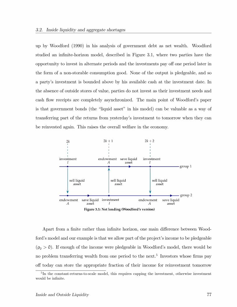
3.2. Inside liquidity and aggregate shortages
up by Woodford (1990) in his analysis of government debt as net wealth. Woodford
studied an infinite-horizon model, described in Figure 3.1, where two parties have the
opportunity to invest in alternate periods and the investments pay off one period later in
the form of a non-storable consumption good. None of the output is pledgeable, and so
a party’s investment is bounded above by his available cash at the investment date. In
the absence of outside stores of value, parties do not invest as their investment needs and
cash flow receipts are completely asynchronized. The main point of Woodford’s paper
is that government bonds (the “liquid asset” in his model) can be valuable as a way of
transferring part of the returns from yesterday’s investment to tomorrow when they can
be reinvested again. This raises the overall welfare in the economy.
Apart from a finite rather than infinite horizon, one main difference between Wood-
ford’s model and our example is that we allow part of the project’s income to be pledgeable
(ρ0 > 0). If enough of the income were pledgeable in Woodford’s model, there would be
no problem transferring wealth from one period to the next.5 Investors whose firms pay
off today can store the appropriate fraction of their income for reinvestment tomorrow
5In the constant-returns-to-scale model, this requires capping the investment, otherwise investment
would be infinite.
Inside and Outside Liquidity 77
3.2. Inside liquidity and aggregate shortages
by buying a financial stake in firms that invest today and pay off tomorrow; an equity
market would be a perfect substitute for government bonds (this conclusion extends to
uncertain payoffs.) However, if the pledgeable income drops below the cost of investment
(ρ0 < 1 < ρ1) there will again be a role for outside liquidity in Woodford’s model: an
equity market will not work if the pledgeable income is too small.
The general message here is that the problem of partial pledgeability, which limits
the amount of funds that an entrepreneur can attract, also makes it harder for investors
to supply liquidity. The specific observation that the corporate sector cannot provide
sufficient aggregate liquidity whenever it is a net lender is very general. Even if the
liquidity shocks were uncertain as in section 2.2, as long as I−A < 0 the budget constraint
(2.4) implies that the expected date-1 net return of the corporate sector must be negative,
and therefore that the corporate sector does not have sufficient assets to support the
proposed plan.
3.2.2 Net borrowing: aggregate shocks
Assume now that the corporate sector is a net borrower, I − A > 0, where A is the
aggregate endowment of the entrepreneurs.6 Also, assume that there are only two liquidity
shocks satisfying ρL < ρ0 < ρH with the additional property that the date-1 continuation
investments should take place both when the liquidity shock is high and when it is low
(condition (2.10) is satisfied). Because I−A > 0, the expected net return at date 1 must
be strictly positive or else the budget constraint (2.4) would be violated. However, it is
quite possible that the realized net return is negative in some states and therefore that
there are states with insufficient inside liquidity. Whether this will be the case depends
critically on the correlation of liquidity shocks across firms.
Consider first the extreme case where all firms are technologically identical and hit
6The corporate sector is typically a net borrower, see Mayer (1988). Recently, though, the corporate
sectors in a number of countries (US, UK and Japan in particular and only a bit less in the euro area)
have cut back on total borrowing causing them to run net financial surpluses several years in a row.
Inside and Outside Liquidity 78
3.2. Inside liquidity and aggregate shortages
by the same shock — either all firms experience a high shock ρH > ρ0 or all of them
experience a low shock ρL < ρ0. The high shock occurs with probability fH and the
low shock with probability fL. Of course, when the aggregate shock is low all firms can
continue, because continuation investments are self-financing in that case. For instance,
investors can contractually agree to let a firm in need of liquidity, dilute the initial investors
pro rata so that the amount ρLI can be raised from new investors; alternatively firms may
not contract for liquidity, but rather negotiate with investors for fresh funds when the
liquidity shock arises as discussed in section 2.2. By contrast, no firm can continue when
the high shock hits, because just as in the deterministic case discussed above, every firm
now has a negative continuation value. There are no assets to back up investor promises
to cover a high liquidity shock. The only option is for all firms to close down in the
high-shock state.
3.2.3 Net borrowing: independent shocks
Consider next another extreme case, one where each firm is hit by an idiosyncratic liquidity
shock at date 1. With a continuum of ex ante identical firms the law of large numbers
allows us to treat aggregate variables as deterministic. Assume tentatively that all firms
are able to continue at full scale. The aggregate budget constraint for the corporate sector
is then
fL (ρ0 − ρL) I+ fH (ρ0 − ρH) I ≥ I−A > 0,
implying that
fH(ρH − ρ0)I < fL(ρ0 − ρL)I. (3.2)
The left-hand side represents the aggregate demand for liquidity by “distressed firms”
(negative NPV firms), while the right-hand side is the aggregate supply of liquidity by
“intact firms” (positive NPV firms). Both terms are deterministic, because shocks are
Inside and Outside Liquidity 79
3.2. Inside liquidity and aggregate shortages
independent. We conclude that with independent shocks and a continuum of firms that
are net borrowers at date 0, the productive sector is self-sufficient with regard to liquidity.7
There are many institutional arrangements that support the efficient continuation of
firms when shocks are independent. For instance, one could set up a financial intermediary
that held all the shares of the productive sector and issued claims on this aggregate market
portfolio to individual investors. The financial intermediary would provide liquidity to
firms on a contingent basis: firms with a high shock would get ρHI, and firms with a low
shock would get ρLI.
Another way of ensuring that the firms with a liquidity shortage (facing shock ρH)
benefit from the liquidity provided by the other firms is to have each hold a sufficiently
large share of the stock index.8 At date 0, let each firm buy a fraction β of the stock
index. Let the one-hundred-per-cent date-0 value of the stock index be Vβ. A firm could
borrow [I−A] + βVβ to finance its date-1 investments. Alternatively, a firm could issue
equity and use the proceeds (equal to Vβ because of unit mass) to pay both for the net
investment I−A and its purchase of a share β in the stock index.
At date 1, the representative firm sells its share in the stock index back to the con-
sumers, using the proceeds to cover its liquidity shock ρI. We need to show that β can be
chosen so that the firm can always cover the high shock ρ = ρH. Any surplus from the sale
of the index is distributed as a dividend to the firm’s shareholders at date 1. Adding the
expected date-2 dividend ρ0I to the contingent date-1 dividend provides date-0 investors
with a total payout
βVβ − ρI+ ρ0I.
7This conclusion also holds when firms are heterogenous, as long as they are net borrowers at date
0 and face idiosyncratic shocks. However, if there is a finite number rather than a continuum of firms,
there will always be a positive probability that the supply of liquidity is insufficient. For instance, with
two firms, each facing a high shock with probability 1/2, there is an aggregate liquidity shortage if both
experience a high shock simultaneously, which happens with probability 1/4.8In Holmström and Tirole (1998), we wrongly claimed that holding shares in a stock index would not
always ensure suffient liquidity for individual firms, because some of it would be wasted. We are very
grateful to Ivan Werning for correcting this error.
Inside and Outside Liquidity 80
3.2. Inside liquidity and aggregate shortages
Averaging across firms we get
Vβ = βVβ − (fHρH + fLρL)I+ ρ0I = βVβ + (I−A).
The date-0 shares held by investors (1− β of the index) are therefore worth
(1− β)Vβ = I−A, (3.3)
per firm. Their initial investment is covered so they are indeed willing to get on board.
Finally, note that (3.3) implies that Vβ goes to infinity as β approaches 1.9 Con-
sequently, we can always choose β so that the distressed firms can cover their liquidity
shock:10
βVβ ≥ ρHI.
This reasoning extends to the more general case in which continuation is not second-
best for all shocks. For example, in the continuous version of the model, where the optimal
cut-off ρ∗ exceeds ρ0, but is strictly less than ρ1, some shocks will not be met. We
encourage the reader to check that the reasoning above applies by having firms hold a
share β of the index satisfying
βVβ = ρ∗I
which allows them to cover all shocks up to ρ∗. This way, firms with a shortage of liquidity
9The smaller the outsiders’ share per firm, 1− β, the larger is the one-hundred-per-cent-value of the
firm (Vβ).10Equivalently, the entrepreneurs can buy a fraction β of the stock market such that they just have
enough liquidity when facing a high shock when they have secured the right to dilute initial investors:
(ρH − ρ0)I = βVβ .
Then the date-1 stock market value corresponds to the payoff from intact entrepreneurs:
Vβ = fL [(ρ0 − ρL)I+ βVβ ] ,
or equivalently:
Vβ = fL [(ρ0 − ρL)I+ βVβ ] + fH [(ρ0 − ρH )I+ βVβ ]
= I−A+ βVβ .
Inside and Outside Liquidity 81
3.3. Outside liquidity and liquidity premia
(ρ ∈ (ρ0,ρ∗]) benefit from the excess liquidity of those who either shut down (ρ > ρ∗) or
are able to continue without using outside liquidity (ρ ≤ ρ0).
There are various ways to provide for liquidity when there is no aggregate risk (shocks
are independent). The key is to make sure that there is a mechanism whereby those firms
that do not need all their date 1 liquidity (because of a low shock) will transfer their
excess liquidity to those firms that do need it (because of a high shock). Intermediaries
can handle the job with credit lines and equity markets can do it assuming that firms pay
their dividends and sell their shares of the stock index in the right way.11 By contrast,
suppose that firms just borrow from consumers and do not secure a credit line, nor invest
in shares of other firms. Then distressed firms (with the high liquidity shock) cannot
continue, while the unused liquidity (ρ0 − ρL)I of the intact firms (with a low liquidity
shock) is wasted.
The smaller the pledgeable income ρ0, the less there is inside liquidity and the more
important it is to coordinate liquidity efficiently. The reverse may be more common in
reality: the same problems that cause pledgeable income to be low (e.g. poor corporate
governance and regulatory oversight over financial firms) tend to lead to poor coordination
of liquidity as well (due to underdeveloped financial markets).12
3.3 Outside liquidity and liquidity premia
3.3.1 Fixed supply of outside liquidity
Let us return to the case of aggregate liquidity shocks discussed in section 3.2.2. All
firms are identical and each gets hit by the same liquidity shock, which can be either high
11Cross-holdings are common in some countries (e.g. in Europe and Asia) as a way of maintaining
control of companies with a smaller number of shares than cash flow rights, a practice that many consider
bad corporate governance. Independent companies do not seem to hold shares for liquidity reasons,
probably because the stock index is rather volatile, unlike here. Indeed the stock index is likely to be low
precisely when firms need cash.12There is a large literature linking financial development and growth; see, e.g., Levine (1997), Pagano
(1993) and Rajan and Zingales (1998). Empirical work considers various measures of financial develop-
ment in an attempt to capture the ease of access to funding liquidity.
Inside and Outside Liquidity 82
3.3. Outside liquidity and liquidity premia
(ρH > ρ0) or low (ρL < ρ0). We concluded that all firms could continue in the low-shock
state, but no firm could continue in the high-shock state, because there was no inside
liquidity in that state nor (by assumption) any outside liquidity.
Suppose now that there is an external, deterministic source of liquidity, an asset or a
set of assets that produce LS units of corn regardless of the state of nature (we let the
aggregate payoff be deterministic for expositional purposes.) It will not matter whether
the asset produces corn at date 1 or date 2 or some in both, because consumers are
indifferent between consumption in the two states. In a more liberal interpretation of
“corn”, the asset could be anything that produces value for the consumer, such as real
estate, land, or a natural resource like oil. As we have mentioned before, the outside
liquidity here could also represent a fixed amount of government bonds that are backed
up by the government’s ability to tax consumers.
With the help of outside liquidity, entrepreneurs can save some of their date-0 endow-
ment to insure, at least partially, against a high liquidity shock at date 1. Let q be the
price of a unit of liquidity; that is, the date-0 price of a unit of corn delivered in each of the
two states at date 1. If the supply of outside liquidity, LS, is so large that it can support
the second-best plan described in Chapter 2, q will equal 1. The price of liquidity can
never go below 1, because consumers (who are assumed to have big aggregate endowments
in each period) would then want to postpone all their consumption to date 1. This would
drive the price of the liquid asset to its date-1 value, which is 1. By contrast, the date-0
price q can go above 1, because for firms the value of transferring wealth to date 1 may
well be worth more than 1. The difference q − 1 ≥ 0 is the liquidity premium. Whenthe liquidity premium is strictly positive (q > 1), only firms will buy liquidity at date
0. Consumers do not have a demand for liquidity (but see section 3.4) The spot price of
liquidity at date 1 is of course 1.
The budget constraint of a representative firm that buys ` units of liquidity at date 0
Inside and Outside Liquidity 83
3.3. Outside liquidity and liquidity premia
is
I−A+ (q− 1) ` ≤ fL (ρ0 − ρL) I+ fH (ρ0 − ρH) iH (3.4)
The net cost of liquidity is (q− 1) `, since ` units of liquidity is worth ` at date 1. In
the low-shock state, the firm will and can continue at full scale (iL = I) regardless of
`, because continuation is self-financing. In the high-shock state, a firm needs outside
liquidity to continue.
A firm that buys ` units of liquidity can in the H-state continue at a scale iH ≤ I thatsatisfies the liquidity constraint
iH (ρH − ρ0) ≤ `. (3.5)
Constraint (3.5) assumes that, when necessary, the firm can raise up to iHρ0 at date 1 by
diluting its initial stock (issuing claims that are senior to the initial claims; see section
2.3).
Let us determine the firm’s demand for liquidity. Given the price of liquidity q, the firm
simultaneously chooses its level of liquidity `, the initial investment I, and the continuation
scale iH ≤ I subject to the budget constraint (3.4) and the liquidity constraint (3.5).
Suppose the firm decides not to continue in the high state (iH = 0). Since it does not
need any external liquidity in that case the maximum initial investment level is
I =A
1− fL (ρ0 − ρL). (3.6)
This plan gives the entrepreneur a net payoff
U0 = (ρ1 − ρ0) fLI−A =[fL (ρ1 − ρL)− 1]
1− fL (ρ0 − ρL)A. (3.7)
Suppose instead that the firm in the high-shock state decides to continue at full scale
iH = I. To do so, it has to buy outside liquidity ` = (ρH − ρ0) I. Substituting ` into the
budget constraint (3.4) gives the maximum initial investment
I(q) =A
1+ (q− 1) (ρH − ρ0)− fL (ρ0 − ρL)− fH (ρ0 − ρH). (3.8)
Inside and Outside Liquidity 84
3.3. Outside liquidity and liquidity premia
The entrepreneur’s net payoff is then
U1(q) = (ρ1 − ρ0) I(q)−A =ρ1 − (1+ (q− 1) (ρH − ρ0) + ρ)
(1+ (q− 1) (ρH − ρ0) + ρ)− ρ0A. (3.9)
Here ρ = fLρL + fHρH is the average liquidity shock at date 1.
The firm will continue in the high state as long as U1(q) > U0. Our earlier assumption
fL (ρH − ρL) < 1 implies that U1(1) > U0 (see (2.13)). If q = 1, it is optimal to continue.
Note that U1(q) is a strictly decreasing function. Let qmax be the value at which the firm
is indifferent between continuing and not continuing in the H-state:
U1(qmax) = U0 (3.10)
Using the expressions for U0 and U1(q), we can write this equality as
fL
fH(qmax − 1)(ρH − ρ0) + fL(ρH − ρL) = 1 (3.11)
We can interpret equation (3.11) in the following way. Define the effective unit cost of
investment as the expected cost of bringing one unit of investment to completion. This
value depends on the continuation policy. For a firm that continues in both states the
effective unit cost is
c1(q) ≡ 1+ (q− 1) (ρH − ρ0) + ρ (3.12)
Because the firm always continues, c1(q) is the sum of the initial investment, the net cost
of liquidity per continuation unit in the high state and the expected reinvestment cost at
date 1.
For a firm that does not continue in the H-state the effective unit cost is
c0 ≡ 1+ fLρLfL
(3.13)
Since only a fraction fL of projects are continued, the effective cost in this case is obtained
by scaling the expected cost of a unit investment by the fraction fL.
Inside and Outside Liquidity 85
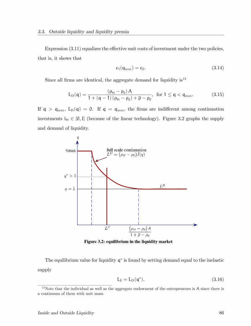
3.3. Outside liquidity and liquidity premia
Expression (3.11) equalizes the effective unit costs of investment under the two policies,
that is, it shows that
c1(qmax) = c0. (3.14)
Since all firms are identical, the aggregate demand for liquidity is13
LD(q) =(ρH − ρ0)A
1+ (q− 1) (ρH − ρ0) + ρ− ρ0, for 1 ≤ q < qmax. (3.15)
If q > qmax, LD(q) = 0. If q = qmax, the firms are indifferent among continuation
investments iH ∈ [0, I] (because of the linear technology). Figure 3.2 graphs the supplyand demand of liquidity.
The equilibrium value for liquidity q∗ is found by setting demand equal to the inelastic
supply
LS = LD(q∗). (3.16)
13Note that the individual as well as the aggregate endowment of the entrepreneurs is A since there is
a continuum of them with unit mass.
Inside and Outside Liquidity 86
3.3. Outside liquidity and liquidity premia
For values LS such that 1 < q < qmax, the liquidity premium is
q∗ − 1 =A
LS−1+ ρ− ρ0ρH − ρ0
. (3.17)
The liquidity premium will be zero if LS exceeds the maximum demand for liquidity,
A(ρH − ρ0)/(1+ ρ− ρ0).
3.3.2 Comparative statics.
Investment scale in response to q.
The firm’s initial investment I is non-monotone in the supply LS. When there is
plenty of outside liquidity the price q = 1 and the firms continue in both states. As
LS decreases, q increases, causing firms to spend more on buying liquidity and less on
the date-0 investment I. At q = qmax firms become indifferent about continuing in the
H-state and the supply LS determines the fraction of firms that continue. The funds no
longer used to buy liquidity will instead be used to increase the initial scale of investment,
leading to a non-monotone relationship between LS and the initial investment I.14
Entrepreneurial wealth and boom-bust cycles.
The easy money that was available to the US corporate sector in the early 2000s seems
to have paved the way for the subsequent liquidity crisis. Our framework suggests a reason
why this may have been the case.
In practice, firms with more resources go for an expansion of scale or for more fragile
investments. While both can easily be modelled in our framework, consider the case of
expanded investment as analyzed in this section. Think of A as the date-0 free (non-
collateralized) cash available to firms. From (3.15), we see that an increase in A creates a
proportional shift in the demand for liquidity LD(q) (for q < qmax). Figure 3.2 then shows
14This non-monotonicity disappears if the firm has two technologies that it can invest in at date 0:
a liquidity producing short-term technology in addition to the long-term technology. In that case, as
LS decreases, more of the firm’s initial investment will flow into the short-term technology, causing I to
decrease.
Inside and Outside Liquidity 87
3.3. Outside liquidity and liquidity premia
that the price of liquid assets q increases. When q reaches qmax, an increasing fraction
of firms start to withdraw their demand for liquidity, implying that they will have to
shut down operations in bad times. As a result, a high supply of liquidity today leads
to a liquidity shortage tomorrow. This can create recurring periods of booms and busts.
(For more on the intertemporal links between liquidity and investment, see Fahri and
Tirole, 2009a, who, in an overlapping-generation model, show how firms that currently
need stores of value can build on older firms’ securities to create liquidity cushions.)
The likelihood of liquidity shortages.
Next let us look at what happens when the probability of the high shock, fH, increases.
We will consider two separate cases: in the first, the change in the probability of a high
liquidity shock occurs before the investment I is made, so I will respond to the change.
There is a long-term effect. In the second case, news about a change in fH arrives after
the investment I has already been made, so I stays fixed as does the purchase of liquidity.
The only impact is on the changed (implicit) price of liquidity after the news.
(a) Long-term effects (I variable). Because
I(q) =A
1+ (q− 1)(ρH − ρ0)− (ρ0 − ρ),
an increase in fH increases ρ and reduces investment. Intuitively the investment is less
profitable, so there is less investment for a given q. Let us also examine how the maximal
price qmax changes with fH. Rewriting (3.11) we have
1+ fLρLfL
= 1+ (qmax − 1)(ρH − ρ0) + ρ
implying that
sign
µdqmax
dfL
¶= sign
µd
dfL
µ1
fL+ fL(ρH − ρL)
¶¶= sign
µ−1
f 2L+ (ρH − ρL)
¶< 0,
since by assumption fL(ρH − ρL) < 1 (that is, there is a liquidity demand when q = 1).
Therefore qmax increases as the likelihood of a high shock (fH) increases.
Inside and Outside Liquidity 88
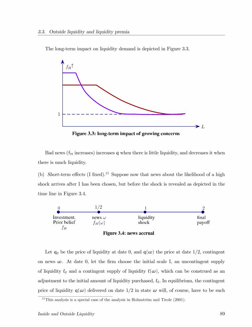
3.3. Outside liquidity and liquidity premia
The long-term impact on liquidity demand is depicted in Figure 3.3.
Bad news (fH increases) increases q when there is little liquidity, and decreases it when
there is much liquidity.
(b) Short-term effects (I fixed).15 Suppose now that news about the likelihood of a high
shock arrives after I has been chosen, but before the shock is revealed as depicted in the
time line in Figure 3.4.
Let q0 be the price of liquidity at date 0, and q(ω) the price at date 1/2, contingent
on news ω. At date 0, let the firm choose the initial scale I, an uncontingent supply
of liquidity `0 and a contingent supply of liquidity `(ω), which can be construed as an
adjustment to the initial amount of liquidity purchased, `0. In equilibrium, the contingent
price of liquidity q(ω) delivered on date 1/2 in state ω will, of course, have to be such
15This analysis is a special case of the analysis in Holmström and Tirole (2001).
Inside and Outside Liquidity 89
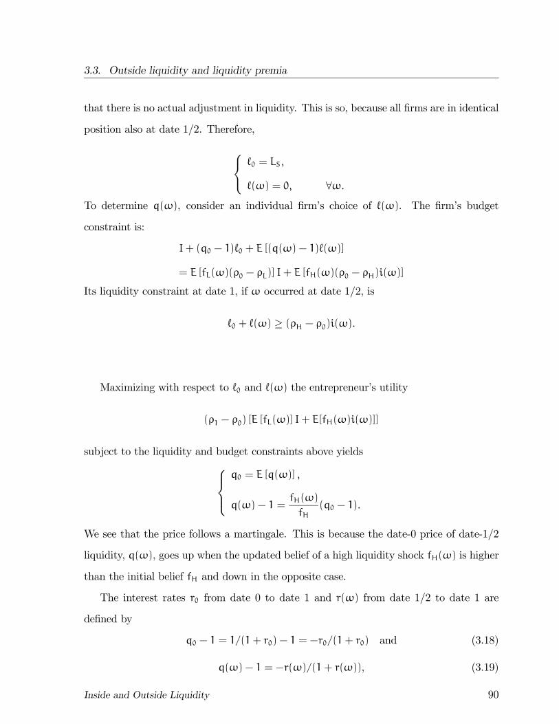
3.3. Outside liquidity and liquidity premia
that there is no actual adjustment in liquidity. This is so, because all firms are in identical
position also at date 1/2. Therefore,
⎧⎨⎩ `0 = LS,
`(ω) = 0, ∀ω.To determine q(ω), consider an individual firm’s choice of `(ω). The firm’s budget
constraint is:
I+ (q0 − 1)`0 + E [(q(ω)− 1)`(ω)]
= E [fL(ω)(ρ0 − ρL)] I+ E [fH(ω)(ρ0 − ρH)i(ω)]
Its liquidity constraint at date 1, if ω occurred at date 1/2, is
`0 + `(ω) ≥ (ρH − ρ0)i(ω).
Maximizing with respect to `0 and `(ω) the entrepreneur’s utility
(ρ1 − ρ0) [E [fL(ω)] I+ E[fH(ω)i(ω)]]
subject to the liquidity and budget constraints above yields⎧⎪⎨⎪⎩q0 = E [q(ω)] ,
q(ω)− 1 =fH(ω)
fH(q0 − 1).
We see that the price follows a martingale. This is because the date-0 price of date-1/2
liquidity, q(ω), goes up when the updated belief of a high liquidity shock fH(ω) is higher
than the initial belief fH and down in the opposite case.
The interest rates r0 from date 0 to date 1 and r(ω) from date 1/2 to date 1 are
defined by
q0 − 1 = 1/(1+ r0)− 1 = −r0/(1+ r0) and (3.18)
q(ω)− 1 = −r(ω)/(1+ r(ω)), (3.19)
Inside and Outside Liquidity 90
3.3. Outside liquidity and liquidity premia
respectively. Note that r0 and r(ω) are negative. For small changes in the probability,
hence small changes in the interest rates, we see from the equilibrium prices that
|r(ω)| ' fH(ω)
fH|r0 | .
We see that the date-1/2 interest rate moves in proportion to the updated probability of
an unfavorable liquidity shock.
3.3.3 Evidence of a liquidity premium in corporate bond spreads
There is a lot of suggestive evidence consistent with a liquidity premium, but with so many
factors affecting interest rates, it has been hard to make a strong case for a premium. A
study by Krishnamurthy and Vissing-Jorgensen (2006) tries to get around this problem
by analyzing the spread of corporate bond yields over Treasury yields and how that
spread varies with the supply of Treasury bonds. Figure 3.5, imported from their paper,
describes the main finding. The horizontal axis measures the logarithm of the ratio of
U.S. government debt to GDP. The vertical axis measures the spread between AAA rated
corporate bond yields and Treasury yields. The data points are September values from
1925 to 2005.
Inside and Outside Liquidity 91
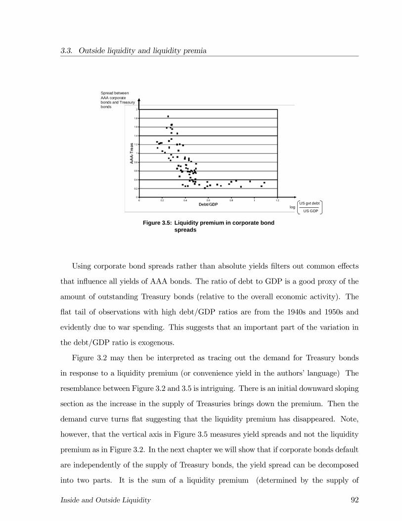
3.3. Outside liquidity and liquidity premia
Figure 3.5: Liquidity premium in corporate bond spreads
Spread betweenAAA corporatebonds and Treasurybonds
logUS gvt debt
US GDP
Using corporate bond spreads rather than absolute yields filters out common effects
that influence all yields of AAA bonds. The ratio of debt to GDP is a good proxy of the
amount of outstanding Treasury bonds (relative to the overall economic activity). The
flat tail of observations with high debt/GDP ratios are from the 1940s and 1950s and
evidently due to war spending. This suggests that an important part of the variation in
the debt/GDP ratio is exogenous.
Figure 3.2 may then be interpreted as tracing out the demand for Treasury bonds
in response to a liquidity premium (or convenience yield in the authors’ language) The
resemblance between Figure 3.2 and 3.5 is intriguing. There is an initial downward sloping
section as the increase in the supply of Treasuries brings down the premium. Then the
demand curve turns flat suggesting that the liquidity premium has disappeared. Note,
however, that the vertical axis in Figure 3.5 measures yield spreads and not the liquidity
premium as in Figure 3.2. In the next chapter we will show that if corporate bonds default
are independently of the supply of Treasury bonds, the yield spread can be decomposed
into two parts. It is the sum of a liquidity premium (determined by the supply of
Inside and Outside Liquidity 92
3.4. Competition for liquidity between consumers and firms
Treasuries) and a risk premium due to the difference in default risk between corporate
bonds and Treasuries (which are essentially default free). Thus, the fact that Treasuries
have a zero liquidity premium in Figure 3.2 when the supply is ample, is fully consistent
with a remaining baseline spread visible in the high debt/GDP observations of Figure 3.5.
3.4 Competition for liquidity between consumers and
firms
Our workhorse model assumes that consumers are patient. Obviously consumers may
themselves demand some liquidity. To consider this and see how our theory works out
a mix of consumer and corporate liquidity demands, this section adds Diamond-Dybvig
consumers (see Appendix 2.2) to the equilibrium analysis as follows. Because consumers
save in the Diamond-Dybvig model, the corporate sector will be a net borrower. The long-
term return that secures the consumers’ future consumption will come from the pledgeable
income of the firms’ illiquid investments. Consumers can be treated as firms that are net
lenders and cannot offer any pledgeable income (their ρ0 is equal to 0).
There are three dates: t = 0, 1, 2.
• Consumers: They are exactly as in Diamond and Dybvig (1983). They invest theirunit endowment at date 0 and receive utility u(c1) from date-1 consumption if they
are impatient (which has probability 1 − α) and u(c1 + c2) if they turn out to be
patient (which has probability α).
• Firms: There is a continuum of identical firms with mass 1. The representative firmhas assets A at date 0 and invests a variable amount I in the long-term project. It
faces a liquidity shock ρ per unit of investment, drawn from a continuous distribution
F(ρ). There is no aggregate uncertainty (the firms’ shocks are i.i.d.).
• Firms can also invest in short-term (liquid) assets. By investing g(`) at date 0, `
units of the good at date 1 can be created, where g0 > 0, g00 > 0, and g0(0) = 1.
Inside and Outside Liquidity 93

3.4. Competition for liquidity between consumers and firms
Letting bρ denote the cutoff for continuing with the long-term project at date 1, the
economy’s resource constraints at date 0, 1 and 2 are:
I−A+ g(`) ≤ 1 (3.20)
(1− α)c1 +hRρ0ρf(ρ)dρ
iI ≤ ` (3.21)
αc2 ≤ F(bρ)ρ0I. (3.22)
Condition (3.20) reflects the fact that the economy’s total endowment, 1+A, is invested
in illiquid (I) and liquid (g(`)) assets. Condition (3.21) highlights how consumers and
firms compete for liquidity at date 1. Finally, (3.22) states that the consumers’ long-
term consumption comes from firms with limited pledgeable income (unlike the model in
Appendix 2 2, where all income was pledgeable).
A Pareto optimum among consumers and entrepreneurs can be found by maximizing
the representative entrepreneur’s rent:
max`,I,ρ (ρ1 − ρ0)F(bρ)I (3.23)
subject to the resource constraints (3.20)-(3.22) and the representative consumer’s ex-
pected utility exceeding some level U:
(1− α)u(c1) + αu (c2) ≥ U (3.24)
Let λ0,λ1, λ2,λ3 be non-negative Lagrange multipliers corresponding to the constraints
(3.20)-(3.24), respectively. The first-order conditions imply:
u0(c1)
u0(c2)
=λ1
λ2,
F(ρ∗)− λ1
hRρ∗0ρf(ρ)dρ
i+ λ2F(ρ
∗)ρ0 −λ1
g0(`)= 0,
1− λ1ρ∗ + λ2ρ0 = 0.
(3.25)
Inside and Outside Liquidity 94
3.4. Competition for liquidity between consumers and firms
The first condition shows that the consumer’s marginal utilities of consumption may
not be set equal, because the investment technologies allow only limited consumption
smoothing, while satisfying entrepreneurial objectives. The second condition determines
the initial investment scale I, taking into account that ` is chosen so that the marginal
cost g0(`) = λ1/λ0. The last condition determines the optimal bρ = ρ∗.
Straightforward manipulations lead to the following condition for the optimal cutoff
ρ∗:
g0(`)ρ∗ =1+ g0(`)
Rρ∗0ρf(ρ)dρ
F(ρ∗)(3.26)
Condition (3.26) generalizes the standard optimal cutoff rule (ρ∗ = c) to the case of costly
liquidity hoarding. The average cost of bringing one unit of investment to completion for
an arbitrary cutoff bρ becomesc(bρ, q) = 1+ qRρ0 ρf(ρ)dρ
F(bρ) ,
which generalizes condition (2.22) to the case of costly liquidity (q ≥ 1). Letting
q ≡ g0(`),
condition (3.26) can be written in a form analogous to the standard cutoff rule
qρ∗ = c(ρ∗, q),
since qρ∗ is the cost of raising the cutoff level marginally above ρ∗.
Patient consumers help firms “bridge” dates 1 and 2, as they do not demand cash at
date 1. And so the discount factor 1/q between dates 0 and 1 is the only modification to
the formula obtained in Chapter 2.
The Pareto optimal production plan can be decentralized in the following sense. Let
Q = λ2/λ0 be the consumer’s marginal valuation of date-2 consumption relative to the
marginal valuation of the date-0 endowment. The representative firm then solves:
Inside and Outside Liquidity 95
3.4. Competition for liquidity between consumers and firms
max`,I,ρ (ρ1 − ρ0)F(bρ)Isubject to
I+ q` ≤ A+QF(bρ)ρ0I,[
Zρ0
ρf(ρ)dρ] I ≤ `.
which yields the same first-order conditions as in the Pareto program and therefore also
(3.26).
A corresponding decentralization holds for consumers, but requires that the demand
for liquidity be intermediated by banking contracts of the Diamond-Dybvig type (i.e. con-
tracts that provide limited insurance to consumers). The maximization of (1−α)u(c1)+
αu(c2) subject to the budget constraint:
1 ≥ (1− α)qc1 + αQc2
yields
u0(c1)
u0(c2)
=q
Q
which is consistent with the first condition in (3.25).
Our basic model is thus a special case of this model, in which
• consumers are always patient: α = 1
(and so `I
=Rρ∗0ρf(ρ)dρ)
• the consumers’ marginal rate of substitution between dates 0 and 2 is normalizedat Q = 1.
An interesting extension of this framework would consist in assuming that the fraction,
1 − α, of consumers, who face a liquidity shock, and the distribution of the corporate
liquidity shocks are co-determined, i.e., are driven by a common factor. For example, as
in the stylized model of section 5.2 below, workers from closed plants enter unemployment
and face liquidity needs. We leave this extension for future research.
Inside and Outside Liquidity 96

3.5. Endogenous supply of liquidity
3.5 Endogenous supply of liquidity
So far, we have assumed that the supply of liquidity is exogenous. In reality, the private
sector can produce liquidity through a variety of technologies, for instance by investing
in projects with safer and shorter term payoffs. As the liquidity premium rises with
increased demand, the private sector will respond by shifting more resources towards
supplying liquidity.
To illustrate, suppose there is a second sector, the S-sector (for short-term), consisting
of a continuum of identical firms with unit mass. Assume that each entrepreneur in this
sector has an individual endowment AS and access to a linear storage technology that
transforms one unit of corn at date 0 into ρ0S < 1 units of corn at date 1. As well, assume
the short-term project provides a private benefit to the entrepreneur, ρ1 − ρ0, such that
ρ1 > 1. The budget constraint for each firm in this second sector is
lS ≤ AS + qρ0SlS. (3.27)
The plan to invest `S at date 0 must be covered by the sum of the entrepreneur’s own
capital AS and the date-1 return ρ0S`S valued at unit price q. Because ρ1 > 1, the
entrepreneur will invest in the storage technology for all values q ≥ 1. The maximuminvestment scale, implied by the budget constraint, gives the individual (and aggregate)
supply function
`S (q) =ρ0SAS
1− qρ0S. (3.28)
This supply function is strictly increasing and convex with q = 1/ρ0S as an asymptote.
The higher is q, the more liquidity the economy will produce. The marginal cost of
production is decreasing in q. At qmax = 1/ρ0S, the firm becomes self-financing at which
point it can supply an infinite amount of liquidity. For prices below this maximum, the
supply is constrained by the initial capital the entrepreneur has.
Note that the distribution of capital between the entrepreneurs in the two sectors
matters for the amount of liquidity that will be produced as well as for the equilibrium
Inside and Outside Liquidity 97
3.5. Endogenous supply of liquidity
price of liquidity. As the ratio of AS/A decreases, the price of liquidity will rise and the
leverage of AS will grow while the leverage of A will decline.
By contrast, if all entrepreneurs have access to both technologies, the equilibrium
price of liquidity will be such that each entrepreneur is indifferent between operating the
storage technology and selling liquidity to others or operating the long-term technology
and buying liquidity from others (or being self-sufficient by operating both technologies).
If liquidity-producing technologies have faster payoffs, something our model is silent
on,16 the above logic will have the simple prediction that tighter liquidity, as measured
by a higher liquidity premium q−1, will cause the private sector to reallocate investment
funds from long-term to short-term ones. This is one potential explanation for why, in
times of tight liquidity, the maturity of debt shortens.
Expanding private sector liquidity
There are other ways in which the private sector can expand liquidity supply in times
of high liquidity demand. One important means is by expanding pledgeable income ρ0,
which we have so far taken as fixed. There are many ways in which the pledgeable income
can be expanded. For instance, a bank, a venture capitalist or some other intermediary
may be able to monitor the firm, reduce the cost of moral hazard and thereby the illiquid
stake that the entrepreneur needs to hold to keep him from cheating (see Holmström
and Tirole 1997). Or a country may institute a better corporate governance system
with regulatory changes that improve the firm’s reporting or incentives more generally.
Increased transparency and better regulatory mechanisms that protect investors make
it easier for them to recover investments and therefore raises ρ0 for most firms. In a
dynamic model, reputation effects are often strengthened, reducing the need for financial
incentives. This, too, raises the pledgeable income.
16It does not matter whether the units of corn produced by the firms in the second sector accrue at
date 1 or date 2. The key property is that they are fully pledgeable (liquid).
One might conjecture however that shorter investments, either because they involve less uncertainty and
therefore less adverse selection or because they offer less scope for diversion, have a higher pledgeability
than longer-term ones.
Inside and Outside Liquidity 98
3.5. Endogenous supply of liquidity
Another important determinant of aggregate liquidity is the degree of financial market
development and the extent to which corporate income and private wealth are turned
into tradable assets. When a private firm goes public and its shares become liquid (in the
traditional financial sense), the portfolio of tradable securities expands. Note that even if
the pattern of returns from the new shares can be replicated with available securities on
the market, a public offering can add value if the shares pay off in a state where liquidity
is in short supply. This contrasts with standard financial models where there is no such
effect.
Increased securitization does not necessarily add to the net supply of liquidity, because
the gross increase in the supply of liquidity may be associated with a simultaneous increase
in the demand for liquidity.
Consider the home equity loan market (and other mortgage markets), which offers a
way in which liquidity can be expanded. Mortgaging a fully-owned house through a home
equity loan, makes a non-tradable claim tradable. This adds a savings and investment
instrument to the market, which is valuable if there is a shortage of aggregate liquidity.
The net addition to aggregate liquidity depends on how the mortgage affects the demand
for liquidity. If the home owner invests all of the proceeds from the loan into Treasury
bonds or some similar instruments, little if anything has been added to aggregate liquidity.
Using the proceeds for consumption or real investments, on the other hand, does expand
net liquidity.
Similarly, an IPO may have no consequences for net supply and prices of liquidity, nor
production plans. Suppose the entrepreneur all along knew that he could issue equity to
outsiders and therefore considered the shares of the company a future source of liquidity.
If so, the value of the potentially pledgeable income would be part of his date-1 liquidity in
our model. Taking the company public at date 0 would be a matter of indifference, if the
entrepreneur were to hold equal amounts and an equal distribution of liquidity after the
IPO as before it. If the IPO reduces the efficiency of the firm (because of moral hazard,
Inside and Outside Liquidity 99
3.6. Summary
say), it could even be better to keep the firm private until some event forces an IPO.
The general point here is that the net addition to liquidity is typically smaller than the
gross increase from the IPO, because even privately held assets provide liquidity. After
the IPO, the entrepreneur will likely purchase liquidity to compensate for the loss of the
liquidity embedded in the firm when it was private. Assuming the IPO has no direct
payoff consequences, a public offering in the type of model we have studied, never makes
the liquidity supply worse and typically makes it better. Once the private returns are
turned into publicly tradable claims, some of the liquidity will likely be used to support
other projects than those of the entrepreneur. The market will make more efficient use of
liquidity than if it is privately held.
3.6 Summary
The purpose of this chapter has been to illustrate, in the simplest setting, how a shortage of
liquidity can naturally arise from limited pledgeability of income. This links the familiar
limitations on the debt capacity of firms to the much less discussed limitations on the
funding capacity of investors. The supply problem arises because production of goods also
serves a collateral function.17 The most basic question to ask is whether the corporate
sector generates enough collateral to support the second-best production plans. Put
differently, when is there enough aggregate liquidity to meet corporate needs in each state
of nature?
We have shown that when the productive sector is a net lender, there is always a
shortage of aggregate liquidity. When the corporate sector is a net borrower, the presence
of aggregate liquidity shortages depends on the stochastic structure of the firms’ liquidity
shocks. If all uncertainty is idiosyncratic and there is a continuum of firms, there is always
sufficient aggregate liquidity. In this case, firms can meet their demand for liquidity simply
17Kiyotaki and Moore’s (1997) model of credit cycles turns on this same dichotomy of capital, but in
their model the dual use is within a single firm. Our emphasis is on collateral production for the rest of
the economy.
Inside and Outside Liquidity 100

3.6. Summary
by holding a fraction of the market portfolio. At the other extreme, when there is only
aggregate uncertainty and all firms are hit by the same shock, there is always a shortage of
aggregate liquidity. This creates a demand for outside liquidity, such as government bonds,
which will command a liquidity premium. The liquidity premium declines as the supply
of bonds increases in a manner broadly consistent with the evidence in Krishnamurthy
and Vissing-Jorgensen (2006).
We will later on analyze the role of government and international financial markets
in alleviating liquidity shortages. There are also many ways in which the private sector
can respond to liquidity shortages and high liquidity premia. Firms can change their
production plans; private firms can go public; consumers can increase the leverage on
their homes through home equity loans; and new pledgeable assets can be built. The
subprime crisis may in part have been caused by global shortages of collateral that led to
imaginative, but in the end fragile ways to increase the aggregate supply of liquidity, a
topic we will come back to in the Epilogue.
Inside and Outside Liquidity 101

Chapter 4
A liquidity asset pricing model
(LAPM)
In this chapter we extend the simple model from the previous chapter to a general liquid-
ity asset pricing model (LAPM) with heterogenous firms employing linear technologies
of the sort we have been studying. Uncertainty can affect all the parameters of these
technologies. The model shows how liquidity premia are determined in such a setting,
how they affect bond yields and firm values and how firms plan investments and optimally
manage liquidity risks in light of such premia. We start with the case where there are two
aggregate shocks, before moving on to the general model.
4.1 LAPM with two aggregate shocks
4.1.1 Liquidity premia and bond yields
With heterogenous firms it is more convenient to work with state prices. All asset prices
can readily be recovered from state prices, since markets for claims on date-1 liquidity
(the pledgeable part of output) are complete.
Let sHfH be the date-0 price of one unit of liquidity delivered only in the high-shock
state and let sLfL be the corresponding price of liquidity delivered only in the low-shock
state; here fH and fL are the probabilities of a high and a low liquidity shock, respectively
(fL+fH = 1). Because consumers are indifferent about the timing of consumption, sH and
102
4.1. LAPM with two aggregate shocks
sL ≥ 1. If there is an aggregate shortage of liquidity in the high-shock state, we will havesH > 1. We assume that there is no aggregate shortage of liquidity in the low-shock state
(the corporate sector is self-financing in that state), and therefore sL = 1. The date-0
price q of a unit of unconditional liquidity at date 1 (e.g., a risk-free unit bond, expiring
at date 1) can then be written
q = fL · 1+ fH · sH (4.1)
and the liquidity premium
q− 1 = fH(sH − 1). (4.2)
The yield on a risk-free bond is
κ =1− q
q=
−fH(sH − 1)
1+ fH(sH − 1)≤ 0. (4.3)
The yield is zero whenever the liquidity premium is zero, otherwise it is negative since our
risk neutral consumers do not discount the future. The yield on a bond that can default
is strictly larger than κ. To illustrate, consider a bond, indexed by k, with face value 1
that in expectation pays θkH < 1 in state H and θkL = 1 in state L, that is, the bond
defaults with probability fH. Such a bond commands the date-0 price
qk = fL + fHθkHsH. (4.4)
The yield on the bond is
κk =fL + fHθkH − qk
qk=
fHθkH(1− sH)
1− fH(1− θkHsH). (4.5)
Note that κk−κ > 0, because θkH < 1.1 We can interpret Figure 3.5, describing the spread
between AAA rated corporate bonds and Treasury bonds (Krishnamurthy and Vissing-
Jorgensen, 2006) through the lens of this simple example. For bonds that may default, the
1We have:
κk − κ =fH (1− sH )(θkH − 1)(1− fH )
[1− fH (1− θkHsH )][1− fH (1− sH )]> 0.
Inside and Outside Liquidity 103
4.1. LAPM with two aggregate shocks
average spread should stay strictly positive regardless of the liquidity premium. Variations
in default risk (more generally fHθkH) would move the spread around for a given liquidity
premium. The spread should decrease as the price of liquidity goes down (other things
equal) and reach a constant positive value when the liquidity premium is 0. This is the
sense in which the theoretical Figure 3.2 and the empirical Figure 3.5 match, as suggested
in section 3.3.3.
4.1.2 Asset prices
Liquidity premia will also influence the pricing of firms. With two states, each firm,
indexed by j, is characterized by four numbers ρj0,ρj1,ρjL,ρjH, where ρj0 is the pledgeable
payoff, ρj1 is the total payoff, ρjL is the liquidity shock in the low aggregate state, and
ρjH is the liquidity shock in the high aggregate state; all the numbers are per unit of
investment. For simplicity, we assume that there are only two types of firms, "regular"
firms and "contrarian" firms, and that ρjL = 0 for both types. Regular firms demand
liquidity in the high aggregate state H:
0 = ρjL < ρj0 < ρjH < ρj1.2 (4.6)
Contrarian firms, in contrast, supply liquidity in the high aggregate state (for them ρjH <
ρj0). The fraction of contrarian firms is small enough that there still is a shortage of
liquidity in the H-state.
At date 0, each firm j chooses an initial scale of investment Ij and the scale of date-1
continuation investments ijL, ijH ≤ Ij. Since a regular firm is self-sufficient in state L,
such a firm will choose ijL = Ij. We assume, as before, that (ρjH − ρjL)fL = ρjHfL < 1
holds for regular firms, so that continuation at full scale is optimal for them also when
the high shock hits if the liquidity premium is zero (see (2.13)). For contrarian firms,
ijL = ijH = Ij, since they never demand liquidity.
2Recall that these parameters must be such that investment is not infinite. A sufficient condition for
this to be the case is that fL(ρj0 − ρjL) = fLρj0 < 1.
Inside and Outside Liquidity 104
4.1. LAPM with two aggregate shocks
To simplify notation, define the net (financial) payoff of firm j in state ω
yjω ≡ (ρj0 − ρjω)ijω ω = L,H. (4.7)
This is also the amount of liquidity that firm j supplies in state ω (if yjω is negative, the
firm demands liquidity in state ω).
Firm j’s budget constraint is
Ij −Aj ≤ fLyjL + fHyjHsH ≡ Ej(y · s). (4.8)
The right-hand side of the budget constraint, Ej(y · s), is the date-0 market value of thefirm. The investor’s expected date-1 payoff from firm j is
Ej(y) ≡ fLyjL + fHyjH. (4.9)
The liquidity premium of firm j is
νj ≡ fHyjH(sH − 1). (4.10)
The liquidity premium is negative for regular firms (yjH < 0) and positive for contrarian
firms (yjH > 0). Since the budget constraint must bind, we have
Ij −Aj = Ej(y · s) = Ej(y) + νj, (4.11)
or equivalently
(Ij −Aj)− νj = Ej(y · s)− νj = Ej(y). (4.12)
The right-hand side of (4.12) is the investors’ gross expected return at date 1. The
left hand side is their total investment, showing that for a regular firm, which demands
liquidity in the high state, the total investment consists of two parts: the investors’
contribution Ij − Aj towards the initial investment plus the payment of the liquidity
premium −νj > 0 for securing the desired date-1 liquidity.
Inside and Outside Liquidity 105
4.1. LAPM with two aggregate shocks
Define a unit claim on the firm as a claim that in expectation pays 1 at date 1. The
date-0 value of a unit claim on the firm is
qj =Ej(y · s)Ej(y)
=fLyjL + fHyjHsH
fLyjL + fHyjH. (4.13)
When we compare firm values, qj is the natural measure to use. It tells us how much
investors are willing to pay for the asset per unit of return at date 1 net of the liquidity
premium/discount.
Finally, we introduce normalized net state payoffs for firm j
yjω ≡ yjω
Ej(y), ω = L,H. (4.14)
This normalization makes net state payoffs have unit expected value. The value of a unit
claim on the firm can then be written
qj − 1 = fHyjH(sH − 1). (4.15)
Regular firms demand liquidity in the high shock state, so their unit claim features a
liquidity discount (qj − 1 < 0). For contrarian firms, the converse is true (qj − 1 > 0).
The interpretation of the value of a unit claim as an asset price requires some elabora-
tion. At first glance, it would appear that a unit claim cannot sell at a discount, because
consumers (who have limitless wealth) would compete for such claims until the discount
would be driven to zero. So, how can we make sense of (4.15)? The explanation is that,
in the case of a regular firm, the price qj comes with the additional financing obligation to
pay the firm the amount −yjH > 0 in state H at date 1. To secure this commitment, the
investor needs to buy this much liquidity at date 0 at a liquidity premium sH − 1, which
just offsets the liquidity discount qj−1. The total cost of buying a unit claim of a regular
firm is therefore 1. (Recall that consumer income is non-pledgeable so commitments must
be backed up by tradable assets.)
One could interpret this arrangement as a venture capital deal with two stages of
investment. At the initial stage, investors pay qj and at the second stage (date 1), they
Inside and Outside Liquidity 106
4.1. LAPM with two aggregate shocks
pay −yjH if needed, which in expectation costs them 1−qj.3 An alternative arrangement
is to have investors pay 1 per unit for a regular firm at date 0 with the firm investing qj of
it in productive assets and 1− qj in shares of contrarian firms (or other liquid assets). If
the aggregate state turns out to be low, the firm turns the shares of contrarian firms over
to its investors (or sells the shares and pays out the proceeds as a date-1 dividend). If
the state is high, it sells the contrarian shares and uses the proceeds to cover the liquidity
shock. Either way, the expected return on the consumer-investor’s total investment is
zero. However, the price of a share per unit of investment scale at date 0 differs in the
two cases. When everything is paid up front, the price paid at date 0 is 1. When there is
a remaining investor liability, the price at date 0 is given by (4.15), reflecting a liquidity
discount.
Kocherlakota (1996) has argued that in a world where a representative consumer holds
equity either directly or indirectly (through mutual funds, for instance), prices will be
determined by the consumers’ marginal rate of substitution, which in our model always
equals one. This conclusion need not hold when there is segmentation among investors,
as illustrated here.4 If investors pay the full cost of investment up front, letting regular
firms arrange their own liquidity needs by buying shares of contrarian firms, say, the price
of regular firms will equal the marginal rate of substitution of consumers, while the price
of contrarian firms will feature a liquidity premium and consequently no consumer will
buy these shares.
4.1.3 A numerical example
Before proceeding, it may be helpful to go through a numerical example that illustrates the
above analysis. Let the net payoffs of a regular firm j be yjL = 2, yjH = −1 and assume
3For expositions of the staging of venture capital financing, see, e.g., Gompers and Lerner (1999),
Kaplan and Strömberg (2003), and Sahlman (1990).4He and Krishnamurthy (2009) present a model where investment banks are the only ones that can buy
equity and therefore asset prices do not reflect consumer rates of substitution. In empirical work, consumer
segmentation has been used to reconcile equity premia with consumer marginal rates of substitution (see
Vissing-Jorgensen (2002)).
Inside and Outside Liquidity 107
4.1. LAPM with two aggregate shocks
each state has equal probability so that Ej(y) = (0.5). Let the entrepreneur’s date-0
endowment be A = 10. Without aggregate liquidity shortages, the maximum investment
scale would be Ij = A/[1− (0.5)] = 20, of which the investors would contribute 10.
Assume now that there is a liquidity shortage in the H-state and that the liquid-
ity premium in this state is sH − 1 = 0.2. The liquidity premium adds fH(sH − 1) =
(0.5)(0.2) = 0.1 to the cost of each unit of investment at date 0, reducing the maximum
scale of investment to Ij = 10/[(1+0.1)− (0.5)] = 1623. The expected net financial return
at date 1 is therefore Ej(y) = (1623) · (.5) = 81
3. This equals the sum of what the investors
contribute to the initial investment, Ij − A = 1623− 10 = 6 2
3, and what they pay as a
liquidity premium: −νjIj = −(.5)(−1)(.2) · 16 23= 12
3.
Against a date-2 expected pledgeable return of 813, the firm is able to raise 62
3units
from investors at date 0 (all used for the initial investment) with the additional covenant
that investors will promise to cover the liquidity shock at date 1. This covenant costs
investors 813−62
3= 12
3, since they have to buy liquid instruments (e.g. shares in contrarian
firms) to secure their pledge. They could also pay in 813at date 0 and let the firm buy
the requisite liquidity. In either case, the date-0 value of the firm is qj = (623)/(81
3) = 0.8
per unit of expected date-1 return. The firm sells at a discount qj − 1 = −0.2, because
the purchase of liquidity costs 0.2 per unit of expected date-1 return.
4.1.4 The LAPM formula with two states
In the two-state economy, with a liquidity shortage only in the H-state, we find, using
equation (4.15), the following simple relationship between the value of any pair (j, k) of
assets:5
qj − 1
qk − 1=yjH
ykH(4.16)
This valuation formula shows that with a single liquidity shock, the ratio of the liq-
uidity premia (or discounts as the case may be) of any two assets is independent of the
5This valuation formula can be found in Holmström and Tirole (2001).
Inside and Outside Liquidity 108
4.1. LAPM with two aggregate shocks
probability of the state as well as the cost of liquidity and is simply the ratio of the payoffs
in those two states. In particular, we can express the value of every asset in terms of the
price q of a bond that pays one unit in each of the two states. From (4.16) we have
qj = 1+ (q− 1)yjH. (4.17)
4.1.5 Equilibrium determination with two states
In section 3.3.1 we described how the bond price q is established in equilibrium when firms
are homogenous and there are two states. The equilibrium in the case of heterogeneous
firms can be similarly found. Expressed as a function of sH, the demand (or supply)
function for state-contingent liquidity by each firm looks identical to the demand (or
supply) function for the case of homogenous firms. As the price sH rises, a regular firm,
because it demands liquidity (yjH < 0), will reduce its level of investment until it reaches
the point of indifference between continuing in both states or continuing just in the L-
state. A contrarian firm, because it supplies liquidity (yjH > 0), will be able to expand
its investment scale in response to an increase in sH until sH reaches a point where some
firm becomes self-financing. This firm can then supply everyone with liquidity, because
of the constant returns to scale technology.
We can ask which characteristics determine the order in which regular firms will drop
out in the liquidity shortage state as the price of liquidity rises (i.e. the order in which
firms switch from ijH = Ij to ijH = 0 as sH increases). We can also ask which contrarian
firm will be the one that first becomes self-financing.6
In order to determine the critical value sH at which a regular firm drops out in the
H-state (contrarian firms never do), we equate the entrepreneur’s net payoffs when the
firm chooses ijH = Ij and when it chooses ijH = 0. Recall that we assumed ρjL = 0 for all
6Note that these questions relate to comparisons across firms, whose parameters are fixed. It is not a
comparative statics exercise. The only things changing are the price sH and the firm’s investment policies
in response to this price change.
Inside and Outside Liquidity 109
4.1. LAPM with two aggregate shocks
firms. It is easy to verify that a regular firm j will continue in both states if and only if:7
sH ≤ sregjH ≡(1− fLρj0)
fL(ρjH − ρj0)for all j (regular). (4.18)
Here sregjH is the highest value of sH such that a regular firm j is willing to continue in
state H. A regular firm drops out at a lower value sH the higher is ρjH and the lower is
ρj0; a firm with a small pledgeable income and/or a large demand for liquidity in the high
state, will drop out early.8 Note that neither the entrepreneur’s wealth Aj, nor his private
benefit ρj1−ρj0 influence the point at which the firm’s demand for liquidity drops to zero,
because of the linear technology.
As long as a regular firm continues in both states (the inequality in (4.18) holds),
the initial investment Ij decreases with sH. Contrarian firms always continue in both
states. They increase their initial investment as sH increases, since the increased value of
supplying liquidity relaxes the budget constraint. For a high enough liquidity premium,
the budget constraint of a contrarian firm will no longer bind and it becomes self-financing.
This occurs when sH = sconjH satisfies:
fLρj0 + fH(ρj0 − ρjH)sconjH = 1. (4.19)
As soon as one contrarian firm j becomes self-financing, it can supply all firms with
liquidity in the H-state. This puts a second cap on the price of sH:
sH ≤ sconjH ≡1− fLρj0
fH(ρj0 − ρjH)> 0.for all j (contrarian). (4.20)
A contrarian firm becomes self-financing at a lower price sH, the more it supplies liquidity
in state H and the higher is ρj0.
7The right hand side of (4.18) can be derived from condition (3.11) by setting ρjL = 0, substitutingqmax = fL + fHsH and solving for the maximum value of sH such that firm j will continue in both states.
8Recall that we must have fLρH < 1, else it would not be worthwhile for the firm to continue in both
states when sH > 1.
Inside and Outside Liquidity 110
4.2. LAPM — the general case
4.2 LAPM — the general case
In this main section we extend the two-state model to a general equilibrium model with a
finite number of states and a finite number of heterogenous firms, whose linear technology
parameters all can depend on the state of nature. The analysis highlights the close
similarities of our model and the standard Arrow-Debreu general equilibrium model as
well as some key differences.9
Let ω be the state of nature revealed at date 1, f(ω) the probability of ω, and
s(ω)f(ω) the date-0 price of liquidity delivered in state ω (at date 1). As before, all
agents are risk neutral and indifferent about the timing of consumption, which implies
s(ω) ≥ 1, since we use the value of a unit of consumption at date 0 as our numéraire.There are J firms indexed j = 1, ..., J (or more precisely, J types of firms, each of measure
1/J, with j a representative firm). Firm j’s investment plan is Ij, ij(ω), where Ij is
the initial investment, and 0 ≤ ij(ω) ≤ Ij is the continuation investment in state ω.
Firm j’s technology is fully described by the tuple ρj0(ω),ρj1(ω),ρj(ω), where ρj0(ω)
is the pledgeable return at date 2, ρj1(ω) is the total return at date 2 and ρj(ω) is the
reinvestment shock at date 1 — all per unit of continuation investment ij(ω). There is
a strictly positive wedge between the firm’s total output and what can be paid out to
investors in each state, that is, ρj1(ω) > ρj0(ω). For technical convenience, we assume
that
ρj0(ω) 6= ρj(ω), for all j and ω. (4.21)
We also assume that
0 <P
ω∈Ω+j
[ρj0(ω)− ρj(ω)]f(ω) < 1 <P
ω∈Ω+j
[ρj1(ω)− ρj0(ω)]f(ω), for all j, (4.22)
9In Holmström and Tirole (2000), we study a liquidity asset pricing model using a different approach
than in this section. We solve for an equilibrium by treating the corporate sector as a single entity that
maximizes the aggregate entrepreneurial welfare. The technology is quite general, and the analysis richer,
but the approach requires a particular distribution of entrepreneurial endowments for the maximization
to match a competitive equilibrium.
Anther model combining asset pricing with corporate finance is Dow et.al. (2005).
Inside and Outside Liquidity 111
4.2. LAPM — the general case
where Ω+j = ω| ρj0(ω) − ρj(ω) > 0 is the set of states in which firm j supplies liq-
uidity. Assumption (4.22) guarantees that initial investments will be bounded and that
the entrepreneur always prefers to invest his full endowment into the project.10 To see
this, consider an investment plan where firm j continues only in states where it supplies
liquidity. Suppose that s(ω) = 1 for all ω. Then the first term in (4.22) is the maximum
share of the firm’s investment that investors are willing to finance. The balance, which is
strictly positive by (4.22), must be paid out of the endowment Aj. This limits the initial
scale of the firm’s investment, giving the entrepreneur the expected utilityPω∈Ω+
j[ρj1(ω)− ρj0(ω)]f(ω)
1−P
ω∈Ω+j[ρj0(ω)− ρj(ω)]f(ω)
Aj > Aj. (4.23)
We see that it is better for the entrepreneur to invest his full endowment in the firm and
continue in all states where the firm supplies liquidity, than to consume his endowment.
Now, suppose that s(ω) > 1 for some ω. In that case the entrepreneur’s expected
utility, using the same strategy as above, can be obtained by replacing f(ω) in the de-
nominator with s(ω)f(ω) > f(ω). We see that the expected utility is higher than in
(4.23), because investors are willing to pay a larger share of the initial investment, if
the firm only invests in states where it supplies liquidity and some such states carry a
liquidity premium. It is not in general optimal for the firm to invest only in states where
it supplies liquidity. Private benefits may be high enough to warrant continuation even
in states where the firm demands liquidity. However, the entrepreneur will always invest
his full endowment in the firm, because of the linear technology.
Finally, let us introduce a source of outside liquidity in the form of assets Lk, k =
1, ..., K, each providing liquidity Lk(ω) ≥ 0 in state ω. For the equilibrium analysis, we
treat outside liquidity as exogenous, but later on, when we discuss government policy, the
supply of outside liquidity is endogenous.
10Assumption (4.22) is much stronger than needed, but alleviates notation without sacrificing insights.
Inside and Outside Liquidity 112
4.2. LAPM — the general case
The aggregate supply of liquidity in state ω is
LS(ω) =Pj
ρj0(ω)ij(ω) +Pk
Lk(ω). (4.24)
The aggregate demand for liquidity in state ω is
LD(ω) =Pj
ρj(ω)ij(ω). (4.25)
Equilibrium is achieved when prices s(ω) ≥ 1, and the firms’ plans Ij, ij(ω) are suchthat the net aggregate demand for liquidity by the corporate sector satisfies:
Pj
[ρj(ω)− ρj0(ω)]ij(ω) ≤Pk
Lk(ω), ∀ ω. (4.26)
with an equality whenever s(ω) > 1.
Given the prices s(ω), firm j solves the following problem:
maxIj ,ij (·)
Pω
[ρj1(ω)− ρj(ω)]ij(ω)f(ω) (4.27)
subject to
(i)Pω
[ρj0(ω)− ρj(ω)]ij(ω)s(ω)f(ω) ≥ Ij −Aj (4.28)
(ii) 0 ≤ ij(ω) ≤ Ij, ∀ω.
The budget constraint (i) incorporates the purchase of sufficient liquidity to make the
continuation plan ij(ω) feasible in each state ω. As long as the aggregate supply con-
straint is satisfied, as it will be in equilibrium according to (4.26), all the firms’ demands
for liquidity can be met. For this reason, there is no need to include a date-1 liquidity
constraint in the firm’s program. We have written the objective function as the entrepre-
neur’s expected payoff, because it equals the social surplus when the budget constraint
binds. Assumption (4.22) guarantees that this will be the case, as we discussed above.
Inside and Outside Liquidity 113
4.2. LAPM — the general case
Prices. The date-0 price for a unit of the exogenous asset Lk, where the unit is defined
as the amount of asset that in expectation delivers one unit of liquidity at date 1, is given
by
qk =
Pω f(ω)Lk(ω)s(ω)P
ω f(ω)Lk(ω)(4.29)
Because s(ω) ≥ 1 and outside sources of liquidity, by assumption, deliver non-negativeliquidity in each state of nature, the price of the exogenous asset k will be such that
qk − 1 ≥ 0, with a strict liquidity premium whenever the asset supplies a strictly positiveamount of liquidity in some liquidity-constrained state.
We define the date-0 price qj of a unit claim on firm j’s equity, as the amount that the
firm can raise for investment purposes at date 0 per unit of expected return at date 1:
qj =
Pω f(ω)[ρj0(ω)− ρj(ω)]ij(ω)s(ω)P
ω f(ω)[ρj0(ω)− ρj(ω)]ij(ω)=
Ij −AjPω f(ω)[ρj0(ω)− ρj(ω)]ij(ω)
. (4.30)
As described in the two-state case, the logic behind this definition can be understood
as follows. Take the case where a firm always demands liquidity in the states in which
there is an aggregate liquidity shortage (s(ω) > 1). In that case qj < 1. For each unit
that the firm raises from outside investors at date 0, it spends Ij −Aj < 1 on the initial
scale of the investment andP
ω[(ρj(ω) − ρj0(ω))ij(ω)(s(ω) − 1)f(ω)] > 0 on state-
contingent claims that provide date-1 liquidity for continuation investments. The price
qj only reflects the return on the investment in scale. An alternative implementation has
the investors (or their representatives, such as banks) promise to supply the liquidity that
the firm needs at date 1. To back up that promise, investors must go out and buy the
necessary amounts of state-contingent claims at date 0. The firm sets the date-0 issue
price sufficiently below 1 so that investors are able to recoup their additional investment
in state-contingent liquidity. In both of these implementations, the investors’ net return
is 0, despite the fact that qj < 1.
Inside and Outside Liquidity 114
4.2. LAPM — the general case
Suppose now that the firm supplies liquidity in every state where there is an aggregate
shortage and hence qj > 1. The firm benefits from supplying liquidity by being able to
raise more funds for investment than it would in a world where there are no liquidity
shortages. The firm could issue separate claims on its date-1 return and the liquidity
service that its assets provide. Or it could have investors invest in both claims and deal
with the allocation of liquidity through contracts with other firms. However, investors
do not invest in assets that command a liquidity premium for their own sake. Investors
earn a zero net return, while the liquidity premium is determined by the intertemporal
marginal rate of substitution of firms.
Equilibrium. The special structure of the model allows us to recast the equilibrium
analysis in terms of an exchange economy without production. This is useful for under-
standing the underlying structure and convenient for proving existence and efficiency.
The key idea is simple. Instead of viewing the firm as choosing a continuation scale
ij(ω) in state ω, we can think of it as choosing its demand for liquidity `j(ω) in that
state, as defined by:
`j(ω) ≡ [ρj(ω)− ρj0(ω)]ij(ω). (4.31)
In states where ρj(ω)− ρj0(ω) < 0, the firm supplies liquidity.
Recall that we assumed that ρj(ω)−ρj0(ω) 6= 0 for technical convenience (see (4.21)).With the change of variables (4.31), the constraint 0 ≤ ij(ω) ≤ Ij can then be expressedas
0 ≤ `j(ω)
ρj(ω)− ρj0(ω)≤ Ij. (4.32)
Note that this constraint forces `j(ω) to have the same sign as ρj(ω)−ρj0(ω) as required
by (4.31).
Firm j’s payoff in state ω becomes
Uj(Ij, `j(ω),ω) = [ρj1(ω)− ρj0(ω)]ij(ω) =ρj1(ω)− ρj0(ω)
ρj(ω)− ρj0(ω)`j(ω). (4.33)
Inside and Outside Liquidity 115
4.2. LAPM — the general case
For every firm j we assume that there is an upper bound Ij on the initial investment level.
This assumption guarantees the compactness of the set of feasible investments. In the
Appendix we will show that Ij can be chosen so that it does not bind in equilibrium. We
define firm j’s investment set as:
Φj ≡ Ij, `j(·)| 0 ≤ Ij ≤ Ij, 0 ≤ `j(ω)
ρj(ω)− ρj0(ω)≤ Ij for every ω. (4.34)
Note that Φj is determined by primitives alone (including Ij as defined later).
The exogenously given liquid assets Lk(ω) ≥ 0 could be owned by the government andhence indirectly by the consumers and entrepreneurs. For simplicity, we assume that all
of the outside liquidity is owned by the consumers and that the total amount of outside
liquidity is strictly positive:
L(ω) ≡Pk
Lk(ω) > 0. (4.35)
Firm j’s choice problem is
maxIj ,`j (·)
Pω
Uj(Ij, `j(ω),ω)f(ω), (4.36)
subject to
Ij +Pω
`j(ω)s(ω)f(ω) ≤ Aj, (4.37)
and
Ij, `j(·) ∈ Φj. (4.38)
With all consumers identical, the representative consumer solves
maxc0 ,c1 (·)
¯c0 +
Pω
[c1(ω) + c2(ω)]f(ω)
°(4.39)
subject to
c0 +Pω
[c1(ω) + c2(ω)]f(ω) ≤ A0 +A1 +A2 +Pω
L(ω)(s(ω)− 1)f(ω), (4.40)
c0, c1(ω), c2(ω) ≥ 0. (4.41)
Here (A0,A1,A2) are the representative consumer’s endowed incomes in the three
periods. These endowments are sufficiently large so that the price of consumption at each
Inside and Outside Liquidity 116
4.2. LAPM — the general case
date is equal to 1 (the normalized price of date-0 consumption). The endowed incomes
are non-pledgeable. By contrast, the liquidity L(ω) that consumers own earns rents
from securing commitments to fund reinvestments. The value of the rent in the budget
constraint is (s(ω)−1)f(ω) per unit. This assumes that L(ω) is not consumed (or rather,
it is capital with a predetermined allocation of consumption benefits, which cannot be
reallocated). The reason we use this formulation is that consumption out of L(ω), which
also can act as collateral, would have to be treated separately from consumption out of
non-pledgeable endowmed income. This would add notation, without changing anything
materially.
The economy’s resource constraints are:
At date 0:
c0 +Pj
(Ij −Aj) ≤ A0. (4.42)
At date 1:
c1(ω) +Pj
ρj(ω)ij(ω) ≡ c1(ω) +Pj
ρj(ω)`j(ω)
ρj(ω)− ρj0(ω)≤ A1, for every ω, (4.43)
At date 2:
c2(ω)−Pj
ρj0(ω)ij(ω) ≡ c2(ω)−Pj
ρj0(ω)`j(ω)
ρj(ω)− ρj0(ω)≤ A2, for every ω. (4.44)
The consumers’ date-0 endowment is allocated between consumption and the firms’
initial investments. The consumers’ date-1 endowment is allocated between consumption
and the firms’ reinvestments. Finally, at date 2, the consumers consume their date-2
endowment and the pledgeable income of firms. We have not included in these constraints
the entrepreneurs’ consumption, since it is a private benefit that cannot be reallocated.
Inside and Outside Liquidity 117
4.2. LAPM — the general case
In addition to the standard resource constraints, there is a constraint on the amount
of aggregate liquidity (collateral) that is available in the economy in each state:
Pj
`j(ω) ≤ L(ω), for every ω. (4.45)
The liquidity constraints limit date-1 reinvestments, which have to be backed up by col-
lateral.
We have transformed our original economy with production into a relatively standard
exchange economy, in which firms solve the program (4.36)-(4.37), the representative con-
sumer solves the program (4.39)-(4.40) and the economy’s aggregate resource constraints
are (4.42) through (4.45).
Because the prices of consumption at dates 0, 1 and 2 are all equal to 1, the only non-
trivial equilibrium prices, s(ω), are associated with the aggregate liquidity constraints
(4.45). An equilibrium is achieved when complementary slackness holds: For every ω, (i)
s(ω) = 1, if constraint (4.45) is slack and (ii) if s(ω) > 1, constraint (4.45) binds. We can
solve for the equilibrium prices s(ω) without explicitly considering consumer decisions,
since consumers do not care about the timing of consumption. Their consumption is
simply determined by the resource constraints (4.42)-(4.44) once we know s(ω).
The existence of equilibrium is proved in the Appendix. The main step in the existence
proof is to show that prices and investments are bounded. We have s(ω) ≥ 1, because ofthe particular consumer preferences and our choice of units (date 0 unit of consumption
has value 1). On the other hand, for each ω, there is a price s(ω) such that whenever
s(ω) > s(ω), all firms stop demanding liquidity in state ω (set `j(ω) ≤ 0) regardless ofthe other prices s(ω0), ω0 6= ω. We also show that the initial investments Ij are bounded
by the amount that could be invested by firm j, if all of the economy’s resources were
devoted to maximizing Ij. This amount is finite, because we have assumed that every
unit invested in a firm requires some amount of entrepreneurial endowment (see (4.22)).
In the Appendix we also show that the equilibrium is constrained efficient in the sense
Inside and Outside Liquidity 118
4.3. Risk management
that there does not exist a plan of consumption and investment that satisfies the aggregate
resource constraints (4.42) - (4.45), in which every entrepreneur and the representative
consumer are as well off as in the price equilibrium, with at least one of them strictly
better off. Note, especially, that even the social planner’s allocations have to satisfy the
aggregate liquidity constraint (4.45); the social planner cannot circumvent the fact that
contingent reinvestment decisions must be backed collateral.
More general technologies. It is straightforward to extend the model and proofs of
existence and efficiency to the case where each firm has access to more than one linear
technology. A firm would then have to solve a more complicated linear program to de-
termine how it should allocate its funds among the available technologies. Because the
optimization takes place against a single resource constraint — the budget constraint — the
solution will generically allocate all the capital to a single technology. The active tech-
nology will vary as the price vector s(·) varies. Since each technology will be associatedwith its own private benefit, private benefits as well as the resource costs will determine
how much liquidity a firm demands or supplies. In response to an increased liquidity pre-
mium in a state ω, a firm will switch towards a technology that produces more liquidity
in that state, giving up private benefits for the value of liquidity. Technologies with a
smaller wedge between pledgeable and private income — for instance, technologies with
more established (or earlier) cash flows or tangible assets would be favored.
4.3 Risk management
Traditional models of asset pricing, such as the CAPM, cannot explain why firms buy
insurance against fires or other casualties, nor can these models provide much guidance
on how firms should manage risk in general. The basic problem is that risk can just as
well be managed by individual investors. Of course, there might be some scale advantages
from having a firm deal with some of the risks it faces, but it seems implausible that these
advantages would warrant the extensive attention to risk management that firms devote.
Inside and Outside Liquidity 119
4.3. Risk management
Firms do not buy only casualty insurance. They also spend large amounts of time and
money on hedging against adverse financial risks like defaults, exchange rate shocks and
other price fluctuations. Decisions on how much cash to keep on hand to cover unexpected
liquidity needs and how to deal with fluctuations in the stock of cash are matters that
the management agonizes over a lot. In the traditional theory they need not do that.
The liquidity asset pricing model developed in this chapter is a small step away from
complete markets, but big enough to explain why firms care about liquidity and to give
some insights into the way risk should be managed. However, as will become clear below,
a full account of hedging and other risk management strategies must necessarily address
implementation problems that depart even further from the standard model.
The perspective underlying LAPM is that firms should consider risk management a
part of liquidity management. This means that risk should be managed jointly with the
firm’s investment decisions so that sufficient liquidity is assured throughout the planning
horizon in the most cost effective way, and so that the cost of capital in future states
guides the firm’s investment plan. This perspective is not new. Froot et al (1993) have
also analyzed the joint determination of financing and investment using an explicit agency
model. One element that is new in our approach is that LAPM places the discussion in an
equilibrium context where the price of liquidity influences risk management and conversely.
Also, much of the Froot et al (1993) analysis is devoted to imperfect implementation of
optimal risk management strategies rather than to fully contingent policies as discussed
here.11
Before looking at the analytics, let us first consider a concrete question faced by many
firms: Should a firm insure its production facilities against fire or other damage and if so,
how extensively? The answer presumably depends on the cost of insurance. Let us assume
insurance is provided competitively at market determined prices. Given actuarially fair
prices, should the firm buy full coverage? Given that firms are effectively risk averse, as
11Holmström and Tirole (2000) addresses some implementation issues in the same set-up as here.
Inside and Outside Liquidity 120
4.3. Risk management
discussed in Appendix 2.2, one might think full coverage is optimal. On the other hand,
perhaps one should embrace risk, given that a mean preserving spread in the date-1
liquidity shock increases welfare (as shown in section 2.4).
In practice, risk management policies typically recommend that “external” risks like
a fire be fully insured or hedged. However, when one cannot find instruments that are
perfectly correlated with the risk, hedging should be partial.12
The message from LAPM is rather different. The amount of hedging depends on
whether risk affects the productivity of the firm or just the liquidity constraint.13 Events
that only influence the date-1 income of the firm, but not continuation investments, should
be fully insured provided that current income is uncorrelated with future income.14 On
the other hand, an event that affects the productivity of the firm’s date-1 investment will
in general be partially rather than fully insured. A fire may fall in either category as
discussed below.
To explain these conclusions let us return to the model with general shocks described
in section 2.5.15 We start by adding state-contingent liquidity prices to the model and
after that introduce shocks to productivity. The basic problem is as before to decide the
level of the date-0 investment I and the date-1 continuation scale i(ω) in all states ω.
These decisions are solved by the program
12For a list of reasons why hedging should be partial rather than complete, see chapter 5 in Tirole
(2006).13We are assuming here that firms have access to insurance in every state, albeit at a potentially high
price.14Suppose that a high profit at date 1 is good news about the date-2 profit (as in de Marzo et al.,
2009, or Tirole, 2006, pp.217-218). Then date-1 reinvestment is more desirable when date-1 profit is high.
This pattern may be implemented in a variety of ways. A natural one is to partially hedge at date 0 the
date-1 profit so as to provide the firm with more liquidity when its profits are high. Alternatively, the
date-1 profit shock may be neutralized (fully hedged), provided that the firm receives a credit line that
is indexed to the realization of profit.15Note that the model in section 2.5 is more general than the formulation we have used here, as it
includes date-1 income of two kinds and also a positive value of liquidation. The proof in the Appendix
can be extended to cover existence of equilibrium and constrained efficiency in this more general set-up.
Inside and Outside Liquidity 121
4.3. Risk management
maxI,i(ω)
Zb(ω)i(ω)dF(ω), (4.46)
subject toZ[(ρ0(ω)− ρ(ω))i(ω) +w(ω)(I− i(ω))]s(ω)dF(ω)
+
Z[r(ω)I+ y(ω)]s(ω)dF(ω) ≥ I−A, (4.47)
0 ≤ i(ω) ≤ I, for every ω. (4.48)
As in section 2.5, we have replaced the parameter ρ1(ω) with the entrepreneur’s private
benefit b(ω) = ρ1(ω) − ρ0(ω), to separate the effect that ρ0(ω) has on the objective
function from its effect on the budget constraint. Recall that the variable w(ω) is the
liquidation value of a unit of initial investment at date 1, r(ω) is the date-1 income per
unit of investment, and y(ω) as the income from old assets in place, which therefore does
not depend on the initial investment.
Let 1+ λ ≥ 1 be the shadow price of the budget constraint. The choice of i(ω) is thendetermined by the sign of
Ψ(ω) = b(ω)− (1+ λ)s(ω)[ρ(ω) +w(ω)− ρ0(ω)] (4.49)
as follows:
i(ω) = 0, if Ψ(ω) < 0
i(ω) = I, if Ψ(ω) > 0
i(ω) ∈ [0, I], if Ψ(ω) = 0.
Shocks to income at date-1 take the form r(ω)I + y(ω). Since income shocks only
affect the budget, they do not directly affect the continuation rule i(ω). There is an
indirect effect through the budget and the return to the initial investment I, but these
effects only depend on the expected values E[s(ω)r(ω)] and E[s(ω)y(ω)]. All income
Inside and Outside Liquidity 122
4.3. Risk management
shocks with the same weighted expected costs will lead to the same investment decisions
and continuation rules. We interpret this as a case where income shocks are treated as if
they are fully hedged, that is, income is as if it were constant.
Compared with a situation where there is ample liquidity in all states (s(ω) = 1 for
all ω), the full distribution of (the components of) the income shock, including their
correlation with s(ω) will matter for firm decisions, because it affects the cost of capital
λ. However — and this is the key point — the change in λ will affect every contingent
decision, not just the decision in state ω. There is no sense in which one can associate
the continuation decision in a state with the total income in that state. Continuation
decisions are determined by Ψ(ω), which does not directly depend on the income.
The continuation index Ψ(ω)measures the entrepreneurial value of continuing in state
ω. The only change in the continuation rule compared to the case where there are no
liquidity shortages comes from a positive liquidity premium s(ω) − 1 > 0. The cost
of capital now varies with the state ω, whereas before it was constant. Economically,
liquidity premia are of course critically important. They influence the firm’s investments
as well as repayment plans and therefore what kinds of securities the firm should issue to
the investors. Other things equal, firms want to repay investors in states where liquidity
premia are high and continue investments in states where they are low.16 As before, only
the sum ρ(ω)+w(ω)−ρ0(ω) of the liquidity shock, the liquidation value and (minus) the
pledgeable income matters for the continuation decision, but now the importance of this
sum relative to the private benefit depends on s(ω) with the weight on the private benefit
b(ω) reduced in states with liquidity premia. The liquidation value is an opportunity cost
exactly on par with the liquidity shock or a shock to pledgeable income.
Let us return to the fire insurance question, looking at it through the lens of (4.49).
If a fire destroys some property, a building say, it is different from a shock to income,
16In Froot et al (1993), the a firm’s optimal state-contingent plan manages liquidity so that the marginal
value of future investments (in our model, continuation investments) are equalized across states.
Inside and Outside Liquidity 123
4.3. Risk management
because in addition to repairing the building there is the option to abandon it. The
financial impact of a fire could take many forms, each affecting differently the decision
to continue. Suppose the building is essential for production and the cost of repairing it
is proportional to the scale of reinvestment. In that case there would be an additional
liquidity shock per unit of investment eρ(ω) so that the total per-unit cost of continuingwould become ρ(ω) + eρ(ω). In states where there is no fire we would have eρ(ω) = 0.Assuming, for simplicity, that the cost of abandoning the building is zero, this case is
then equivalent to a change in the distribution of the liquidity shock. The structure of
the continuation rule would be as in (4.49) but with a change in λ due to the expected
cost of covering the fire in some of the states. Even when the cost of the fire is constant
(eρ(ω) = cfire > 0, when there is a fire), there may be states in which the building willbe abandoned if there is a fire, because it happens to occur in a state with a high cost of
capital. The optimal continuation rule would not insulate the firm against a fire.
The upshot is that, in contrast to income shocks, shocks to productivity will in general
not be fully insured. Correlations between eρ(ω) and s(ω) matter for this reason, but notbecause of any desire to hedge risks as such. Of course, one can also imagine a situation
where rebuilding is always desirable and therefore insurance against a fire will be complete.
The conclusions above, while providing some insights into risk management and in-
surance, also suggest that risk management is linked fundamentally to implementation
problems of the sort discussed in section 2.3. When investors cannot observe the shocks
experienced by firms, insurance against fires, exchange rate fluctuations and related “ex-
ternal” shocks may become more desirable as a way to control the amount of liquidity
the firm has available for reinvestments at date 1. To illustrate the point, let us go back
to our basic model with a continuum of liquidity shocks (section 2.4), where there never
was a shortage of liquidity (so s(ω) = 1 for all ω), where liquidation was worth zero,
where there was no kind of date-1 income, and where the only uncertainty concerned the
cost of reinvestment ρ(ω). In this basic model, the second best was characterized by a
Inside and Outside Liquidity 124
4.4. Concluding remarks.
cut-off rule ρ∗ (0 < ρ∗ < ρ1) such that the firm continued at full scale if and only if
ρ ≤ ρ∗.17 Even if the investors did not observe the liquidity shock, the second best could
be implemented by providing the firm with a credit line up to ρ∗; since the firm had no
alternative use for funds, it would only use the credit line up to the amount needed to
continue at full scale. Now add an income shock y(ω) to this set up. A cut-off rule ρ∗
will still be optimal (though not necessarily the same cut-off as without y(ω)), because
the optimal decision rule fully insures against variations in the income y(ω), as we saw
earlier in the chapter. However, if investors cannot contract on y(ω), the entrepreneur
would invest ρ(ω)i(ω) = max(ρ∗I + y(ω), ρ(ω)I at date 1, since he always wants to
continue at the maximum feasible scale (constrained either by the initial investment or
the available funds). In particular, he would invest a positive amount even if ρ(ω) > ρ∗,
provided y(ω) > 0 and he would be unable to go ahead at full scale even if ρ(ω) < ρ∗,
if y(ω) < 0.
4.4 Concluding remarks.
The essence of our approach to liquidity is based on the twin assumptions that (i) there
is a wedge between total income and pledgeable income and (ii) fully state-contingent
contracts can be written on the pledgeable part of the income. This chapter has shown
how these two assumptions make it both natural and relatively straightforward to carry
out an asset pricing analysis that closely parallels that of an Arrow-Debreu economy.
Despite a close formal analogy, the LAPM equilibrium differs from an Arrow-Debreu
equilibrium in interesting ways. Notably, asset prices can exhibit liquidity premia. Since
we assumed that consumers are risk neutral and indifferent about the timing of their
consumption, liquidity premia are entirely driven by the corporate demand for liquidity.
This segments investors into two: corporate entrepreneurs, who are willing to pay a
17The continuum of states assumption is inconsequential for the point we want to make. Even with a
finite number of states, as we have in this chapter, the second best is characterized by a cut-off rule if
the other assumptions of the basic model in section 2.4 hold.
Inside and Outside Liquidity 125
4.5. APPENDIX. Existence and efficiency of equilibrium.
premium, and investor-consumers, who are not.18
Liquidity premia affect the way corporations hedge risks and plan their investments,
as discussed in the section on risk management. The most important message here is
that, provided that income shocks are serially uncorrelated and independent of the firm’s
actions — that is, there is no moral hazard at date 019 — income shocks should be fully
hedged, because for the budget only the expected value of income matters. By contrast,
shocks to productivity are not fully neutralized. It is states of low productivity rather
than low income that determine whether investments should be continued. As we noted,
these conclusions are critically dependent on fully contingent contracting. If markets are
incomplete, then hedging will typically be incomplete also for income shocks.20
Liquidity premia and the way they influence corporate investment and funding deci-
sions (the issuing of securities) will play an important role when we go on to study the
optimal use of outside liquidity both by the government and by international investors.
4.5 APPENDIX. Existence and efficiency of equilib-
rium.
We prove existence without consumers, since consumers play no material role in determin-
ing equilibrium prices. The consumer is only relevant for proving constrained efficiency,
because of the rents enjoyed from owning L(ω).
18This claim needs a qualification. As we have discussed in this chapter, there are implementations
of a firm’s investment plan, where investor-consumers buy liquidity at a premium in order to back up
promises of future payments. But this is not driven by a consumption demand for liquidity, but rather
by the firm’s demand for liquidity, that is, by segmentation.19See Rochet and Tirole (1996) for an extension of our model to one with date-0 moral hazard affecting
date-1 profitability.20For more on this, see Froot et al (1993) and Holmström and Tirole (2000).
Inside and Outside Liquidity 126
4.5. APPENDIX. Existence and efficiency of equilibrium.
4.5.1 Existence.21
Our approach to existence is standard. We first define compact, convex choice sets, then
a mapping from the product space of choices and prices into itself, which has a fixed point
by Kakutani’s theorem. Finally, we show that the fixed point is an equilibrium.
Define the price space S = s(·)|1 ≤ s(ω) ≤ s(ω), for every ω, where the upperbound s(ω) is chosen so that
s(ω) > maxj
ρj1(ω)− ρj0(ω)
ρj(ω)− ρj0(ω). (4.50)
Note that S only includes the state-contingent prices at date 0, since the price of the
date-0 good was normalized to 1. The upper bound s(ω) ensures that aggregate demand
for liquidity in state ω will be zero if s(ω) = s(ω), regardless of the other components
of s(·). To see this, suppose that firm j demands a positive amount of liquidity `j(ω) > 0when s(ω) = s(ω). Consider an alternative plan where: (i) the firm reduces the demand
for liquidity in state ω to 0; (ii) the entrepreneur reduces his investment in the firm by
the amount `j(ω)s(ω)f(ω) and consumes it instead; and (iii) the investors increase their
date-0 investment so that it exactly off-sets the entrepreneur’s reduced investment. With
these changes the budget will continue to balance, since the amount the entrepreneur has
withdrawn is exactly the date-0 cost of the amount that investors were expected to invest
in state ω in the original plan. Entrepreneurial consumption at date 0 is not optimal, of
course, but it gives a lower bound on the value of the alternative plan. The benefit of the
alternative plan is the entrepreneur’s date-0 consumption value `j(ω)s(ω)f(ω). The cost
of the alternative plan is the entrepreneur’s loss of the private benefit in state ω. The
expected net benefit of the alternative plan is therefore:
`j(ω)s(ω)f(ω)−[ρj1(ω)− ρj0(ω)]`j(ω)f(ω)
ρj(ω)− ρj0(ω)> 0, (4.51)
21We are grateful to Philip Reny for comments on this section.
Inside and Outside Liquidity 127
4.5. APPENDIX. Existence and efficiency of equilibrium.
where the inequality comes from (4.50) and the assumption that `j(ω) > 0. We conclude
that a strictly positive liquidity demand by firm j (hence any firm) cannot be optimal if
s(ω) = s(ω).
Let the set I = Φ1 × ...× ΦJ be the space of investments and liquidity demands by
firms, where
Φj ≡ Ij, `j(·)| 0 ≤ Ij ≤ Ij, 0 ≤ `j(ω)
ρj(ω)− ρj0(ω)≤ Ij for every ω.
Let us define the upper bounds on initial investments, which were left unspecified earlier.
For firm k, let Ik be the highest level of investment that it could achieve if all of the
economy’s resources were devoted to maximize Ik.That is, let Ik solve
maxIj ,`j (·)
Ik (4.52)
subject to (4.53)
−Pj
Pω
`j(ω)f(ω) ≥ Σj(Ij −Aj), (4.54)
0 ≤ ij(ω) ≤ Ij for all .j. (4.55)
Note that this program does not impose any liquidity constraints, just the aggregate
budget constraint for the corporate sector (4.54) and the technological restrictions on
continuation investments ij(·). The aggregate budget constraint for the corporate sectordoes not include L(ω), which the consumers own. Given assumption (4.22), this program
has a maximum. In fact, no firm other than k will be assigned a positive level of investment
in the above program. The optimal plan will devote all of the aggregate endowment to
firm k’s investment. Any investment into a firm j 6= k consumes some of the aggregateendowment, reducing resources for Ik.
We will see that the aggregate budget constraint cannot be violated in equilibrium,
guaranteeing an interior solution if we choose as the upper bounds so that Ij > Ij for all
j.
Inside and Outside Liquidity 128
4.5. APPENDIX. Existence and efficiency of equilibrium.
Define the mapping ϕ : S×I→S×I in the standard way. For every selection of pricess(·) in S, firms solve program (4.36) - (4.38), which determines the range of ϕ in I. Andfor every selection of investment decisions (Ij, `j(·)) ∈ Φj in I, the range of ϕ in S is
defined by the set of prices s(·) that maximize the value of the excess demand for liquidity[Σj`j(ω)− L(ω)]s(ω). This mapping is upper hemi-continuous, since firms solve a linear
program with choices from a compact, convex set.
Let s∗(·), I∗j , `∗j (·) be a fixed point of ϕ. Such a point exists according to Kakutani’stheorem.
We already argued that if s∗(ω) = s(ω) for some ω, aggregate demand for liquidity
would be zero in state ω, implying that there would be an excess supply of liquidity, since
L(ω) > 0. Given the definition of ϕ, this is inconsistent with s∗(ω) = s(ω) being part
of a fixed point. While prices at the fixed point cannot be at their upper bound, some or
all of them can be at their lower bound 1. The definition of ϕ guarantees that s(ω) = 1
whenever there is an excess supply of liquidity in stateω. Only if the demand for liquidity
equals the supply of liquidity can we have an interior price s∗(ω) > 1. We conclude that
at a fixed point, complementary slackness holds, as required by an equilibrium:
[Pj
`j(ω)− L(ω)][s(ω)− 1] = 0, for every ω. (4.56)
Finally, we need to verify that for each firm j, the initial investment Ij is strictly below
the upper bound Ij, when it chooses an optimal plan given prices s∗(·). To do so, we
check that the firms’ optimal plans at the fixed point must satisfy the aggregate budget
constraint (4.54). Multiply the complementary slackness condition (4.56) by f(ω) and
sum over ω. This gives:
Pω
[Pj
`j(ω)− L(ω)][s(ω)− 1]f(ω) = 0. (4.57)
We have then
−Pj
Pω
`j(ω)f(ω) = −Pj
Pω
`j(ω)s(ω)f(ω) +Pω
[s(ω)− 1]L(ω) ≥Pj
(Ij −Aj), (4.58)
Inside and Outside Liquidity 129
4.5. APPENDIX. Existence and efficiency of equilibrium.
The last inequality follows, since the first term in the middle expression is the sum of each
firm’s budget constraint in (4.37) and therefore greater than or equal to Σj(Ij−Aj), while
the second term in the middle expression is non-negative. The economic intuition is that
when s(ω) > 1, some of the budget will be spent on paying for liquidity and therefore
the aggregate budget constraint will be satisfied with slack (the liquidity premium will go
to the representative consumer).
Because the firms’ investment plans at the fixed point satisfy the aggregate budget
constraint, we must have Ij < Ij for every j. Therefore, firms would choose the same
optimal plans without the imposed upper bound on Ij in the feasible setΦj. This concludes
the proof of existence.
4.5.2 Constrained efficiency.
For constrained efficiency, we need to show that a plan that strictly Pareto improves on
an equilibrium plan I∗j , `∗j (·)|j = 1, ...J, given prices s∗(·), cannot be a feasible plan; it
must violate some of the economy’s four resource constraints (4.42) - (4.45). Consider an
alternative plan in which the representative consumer consumes c0, c1(·), c2(·) and thefirms’s invest Ij, `j(·)|j = 1, ...J. Suppose it Pareto improves on the equilibrium plan. In
the equilibrium plan, the budget constraint for each firm must bind, else the entrepreneur
could do better by increasing the initial scale along with some continuation investments.
The budget constraints for consumers must also bind, since otherwise consumers would do
better by increasing their date-0 consumption. Since the alternative plan makes everyone
as well off and some better off, it must violate the sum of the producer and the consumer
budget constraints at the equilibrium prices s∗(·). Formally,
Pj
(Ij −Aj) +Pj
Pω
`j(ω)s∗(ω)f(ω) + c0 +
Pω
(c1(ω+ c2(ω))f(ω) (4.59)
> A0 +A1 +A2 +Pω
L(ω)[s∗(ω)− 1]f(ω).
Consider now the economy’s resource constraints (4.42) - (4.45). Suppose that they
Inside and Outside Liquidity 130
4.5. APPENDIX. Existence and efficiency of equilibrium.
are all satisfied in the alternative plan. Multiply each constraint by the corresponding
equilibrium price (which is 1 for all constraints, except the liquidity constraint (4.45) for
which it is s∗(ω)) and add up the constraints. The result is an expression that is identical
to (4.59) except that the inequality runs in the opposite direction. The assumption that
the alternative plan satisfies all of the economy’s resource constraints is inconsistent with
the plan being Pareto improving. We conclude that the equilibrium allocation must be
constrained efficient. A planner, who must the economy’s resource constraints, including
the liquidity constraints, cannot find an allocation that would be a Pareto improvement
on an equilibrium allocation.
Inside and Outside Liquidity 131

Part III
PUBLIC PROVISION OF LIQUIDITY
132
Chapter 5
Public provision of liquidity in a
closed economy
Chapter 3 demonstrated that the wedge between total returns and pledgeable returns
on investments can create a shortage of instruments for transferring wealth from one
period to the next and thereby make it more costly or even impossible for firms to insure
against future liquidity shocks through credit lines or other forms of advance funding.
The problem reflects an imperfection in the insurance market between consumers and
entrepreneurs. Consumers have the funds needed for insurance payments at date 1, but
the corporate sector may not offer enough financial claims with which consumers can
back up funding commitments at date 0. In the language of the book’s title, there may
be a shortage of inside liquidity (corporate backed claims) in some states of nature. This
creates a demand for outside liquidity. But there is also a waste of potential liquidity in
that consumers who have income may not necessarily dispatch it to the corporate sector
when needed, because the latter is not profitable enough (private insurance has to be
arranged ex ante and not ex post).
In this chapter, we will study the role of government as the sole source of outside
liquidity. The government’s policy can, at an abstract level, be viewed as remedying
the waste of liquidity or, equivalently, as making up for the missing contracts between
consumers and firms.
133
The government supplies liquidity in a variety of forms. Treasury bonds are the most
obvious example. Consumers, firms and especially financial intermediaries use bonds
as savings instruments, as risk sharing instruments and as collateral for complex state-
contingent contracts such as credit swaps, repurchase agreements, and the like. Less di-
rect, but equally important, are all the ways in which the government provides consumer
insurance such as social security, health and unemployment insurance. The government
also takes an active role in securing the functioning of financial markets. Deposit in-
surance, the discount window and various refinancing facilities are examples of on-going
forms of liquidity supply. The recent subprime crisis shows that the government is pre-
pared to provide substantial amounts of contingent liquidity, not just by lowering interest
rates and easing monetary policy, but also by creating new, temporary credit facilities in
an attempt to alleviate systemic disturbances in financial markets. These interventions
can be interpreted as implicit forms of insurance. Our aim is to show that they can be
rationalized within the logic of our model.
As always, one has to ask what enables the government to do more than the private
sector can do on its own. In our view, the key feature that sets the government apart
is its exclusive right to certain decisions, most importantly, the right to tax its citizens.
As a result, the government can make commitments on behalf of consumers, including
generations that are not yet born or actively part of the market. Put simply, the gov-
ernment can act as an insurance broker between consumers and firms, transferring funds
from consumers to producers in states where the net returns from such transfers are high
and making the corporate sector pay for this insurance either ex ante through liquidity
premia on government securities or ex post with corporate taxes. Of course, if there is
a fear that the government may default on its debt or inflate it away, it may be in a
poor position to issue debt, or the debt may end up carrying an unreasonably high price,
making the government’s supply of outside liquidity unreliable or very costly. We will
Inside and Outside Liquidity 134
assume that the government is credible, but that taxation is costly.1
Another way to look at this is to note that consumers are like firms without pledgeable
income (their ρ0 is equal to 0), because they are unable to borrow against their future
income. The state then acts like an intermediary. Through its regalian taxation power,
it is able to transform some of the future income of consumers into pledgeable income
(make their ρ0 positive).2
When and how much funds should be transferred from consumers to producers de-
pends also on the consumers’ liquidity needs. Current generations of consumers may need
liquidity precisely in the states that firms need liquidity. A case in point is unemployment
insurance, which in most countries is taken up by governments and belongs to the set of
automatic stabilizers; were unemployment insurance provided by firms, the (direct plus
indirect) corporate liquidity demand in recessions would be even larger. For the most
part, we will assume that consumer liquidity demand is unrelated to corporate liquidity
demand (or that consumers represent future generations) and leave consumer demand for
liquidity out of the picture, because it complicates the analysis. The exception is section
5.2, which analyzes a highly stylized model of risk sharing between consumers and firms
with the government as a broker.
The chapter is divided into three parts. Section 5.1 focuses on government bonds
and how they should be structured, viewing the issue purely from a liquidity point of
view (the supply of government bonds is of course in the first instance determined by
public finance considerations). Section 5.2 studies optimal risk sharing between firms and
risk averse consumers, mediated by government taxes and subsidies. Section 5.3 gives
two examples of indirect supply of government liquidity — in the first example through
1Kocherlakota (2001) takes exception with the view that the government has special contracting powers
that private parties could not replicate. Instead, he analyzes a model, in some ways similar to ours, in
which the government can improve social welfare by insuring, not the firm, but the financiers of the firm
(they are all depositors, because debt is optimal due to private information). He views this as a rationale
for bailouts, using the banking crisis in Japan as an example.2In the same way that banks raise the pledgeability of borrowers’ income in Holmström and Tirole
(1997), say.
Inside and Outside Liquidity 135
5.1. Public supply of liquidity
unemployment insurance, in the second example by supporting collateral values to avert
a bad equilibrium.
5.1 Public supply of liquidity
5.1.1 Government bonds
The analysis of government supply of liquidity follows closely our analysis of private
supply of liquidity in chapter 3. We continue to use the two-state, variable investment-
scale model from section 2.2, focusing on the case of pure aggregate uncertainty. All firms
are identical and hit by the same shock ρ, which can be high or low with ρL < ρ0 < ρH.
We assume for simplicity that there are no additional private stores of value. When the
high shock ρH occurs, it hits all firms and no firm can continue without outside liquidity.
Firms will nevertheless invest, because the benefits from continuing in the low-shock state
are sufficiently valuable (recall that continuation is always feasible and desirable because
it is Pareto optimal and therefore self-financing in the low-shock state).
We start with the case where the government issues non-contingent bonds at date 0.
The face value of the bond is one unit of corn paid at date 1 regardless of the state of
nature. To be specific, assume that when the government sells a bond at date 0, the bond
is acquired by a firm using the funds available to the entrepreneur at date 0 (this includes
his own funds A and what can be raised from the market). At date 1, if the liquidity
shock is low, the bond goes unused and its value is returned to the investors, who hold the
rights to all pledgeable income. This will allow the entrepreneur to maximize the initial
investment and thus his private benefit. If the liquidity shock is high, the entrepreneur
uses the proceeds from selling the bond to cover the liquidity shock3. Regardless of the
shock, the government will redeem the bond at date 1 by taxing the consumers and paying
the bond holders the face value of their bonds. At date 0, when the bond is issued, the
3An alternative interpretation with the same net outcome has consumers either directly or through
intermediaries buy up bonds to back up pledges to cover a firm’s high liquidity shock.
Inside and Outside Liquidity 136

5.1. Public supply of liquidity
government receives q ≥ 1 per bond and distributes the proceeds to the consumers. Thenet effect of these transactions is that consumers will transfer corn to firms in the high-
shock state, but not in the low shock state. There will also be a net loss of corn due to
the deadweight loss of taxation.
How is the price of the bond determined and how many bonds should the government
issue? The answers to these questions depend on what objective function the government
uses. Credit rationing models raise well-known conceptual problems for welfare analysis.
Even though parties are risk neutral and have identical time preferences over consumption,
Pareto optimal allocations cannot simply be determined by total surplus maximization.
We assume that the government maximizes producer surplus subject to the constraint
that consumers are not made worse off than they would be without the bond issue. This
means that the deadweight cost of taxation will in the end be borne by the corporate
sector and therefore the supply function of the government is determined by the marginal
deadweight cost of carrying out a bond transaction.
Let g(L) be the date-1 cost for the consumer as a function of the amount of bonds L
that the government issues. One should think of the marginal deadweight loss, g0 − 1, as
the marginal cost of public funds, i.e., the cost of distortions embodied in taxation. For
now, assume that the marginal cost g0 is constant. Since the government’s objective is to
keep the consumers’ welfare unchanged, the price of government bonds is set at q = g0.4
At this price, firms can buy as many bonds as they wish. The outcome will be as in Figure
3.2, but with the equilibrium price fixed by q and the equilibrium quantity purchased by
firms determined by the intersection between the government’s horizontal supply curve
and the firms’ aggregate demand curve.
To avoid general equilibrium effects, we assume that the deadweight loss is associated
with date-1 household production that is discouraged by government taxes. At date 0,
4In the general case, with convex g(L), the government will run a surplus when setting the price q
equal to the marginal cost g0. This surplus would have to be distributed back to the firms in somemanner.
Inside and Outside Liquidity 137
5.1. Public supply of liquidity
when the government distributes the proceeds from the bond issue to consumers, there
are no distortionary effects, because there is no production at that date. This makes
the deadweight loss of taxation increase from date 0 to date 1. There is no reason why
it should. Furthermore, it is unlikely to be optimal to shift the full burden to date-1
taxpayers. In general, it will be better to spread the cost of providing liquidity over many
periods and across states of nature (for more on this, see section 5.2). The broad picture,
however, remains the same: when the economy experiences major adverse liquidity shocks,
it may be desirable to transfer funds from the consumers to the corporate sector. These
transfers operate through coercive and distortionary recourse to taxpayer money. While
the government should consider the overall deadweight loss in its fiscal and debt policy,
it can create liquidity that the private sector cannot.
5.1.2 State-contingent bonds
If we were to reintroduce a storage technology, or other short-term private sector tech-
nology, it would appear from the previous discussion that private and public supply of
liquidity would be qualitatively very similar. The two would generally co-exist and the
equilibrium price would be determined by the intersection of the aggregate supply and
demand curves of liquidity. The composition of the aggregate supply would be determined
by the marginal cost of public and private supply, respectively.
This view is misleadingly simple. The government’s actions will naturally influence
state prices as determined in the equilibrium model of Chapter 4. Our arguments do not
take into account these general equilibrium effects. They only reflect the value of marginal
changes.
The view also overlooks a potentially significant advantage that government supplied
liquidity has over privately supplied liquidity. When the private sector invests in a storage
technology that yields a lower composite return than the long-term technology (taking
into account both pledgeable and non-pledgeable income), the value of that liquidity will
Inside and Outside Liquidity 138
5.1. Public supply of liquidity
be wasted if the liquidity shock at date 1 turns out to be low. The problem is that the
private sector often has to decide on the supply of liquidity before the state is known,
whereas the government can wait and see whether the aggregate shock is high or low
before taxing consumers. Only if the aggregate shock is high does the government need
to step in and offer liquidity. This reduces the cost of providing liquidity without losing
any of its insurance benefits. For this reason, the public sector may be able to produce
liquidity more efficiently than the private sector.5
The superiority of contingent over non-contingent bonds.
First, suppose that the deadweight loss of taxing consumers (at date 1) is constant
across states of nature and let λ be the loss per unit of tax raised. We show that the
most effective way for the government to supply liquidity is to issue a state-contingent
bond that pays
1 if the aggregate shock is high, ρ = ρH, and
0 if the aggregate shock is low, ρ = ρL.
To make consumers as well-off as in the absence of a bond, the date-0 price of the
contingent bond should be
qc = fH(1+ λ). (5.1)
Firms will demand contingent bonds as long as the state-contingent price of liquidity in
the bad state in the absence of such bonds satisfies sH > 1+ λ (see Chapter 4).
Compare this with the case of a non-contingent bond. Consumers’ constant welfare
condition requires
qnc = 1+ λ. (5.2)
Let ` ≡ (ρH − ρ0)I denote the amount of liquidity needed in state H (firms do not need
any liquidity in state L). The net cost for the firms is fH(1+ λ)` with a contingent bond
5Throughout this chapter we will set aside commitment, incentive, political economy and other orga-
nizational problems associated with government. To some extent, these could be incorporated into the
shadow price of government funds.
Inside and Outside Liquidity 139
5.1. Public supply of liquidity
and (1 + λ)` − fL` with a non-contingent bond.6 Thus, contingent bonds allow firms to
save
fLλ`. (5.3)
More generally, if λL is the marginal deadweight loss of taxation in the L state, non-
contingent bonds bring an extra surplus fLλL` to the firms. It is only when taxation is
non-distortionary in the low state (relative to date 0 — see the discussion in subsection
5.1.1) that non-contingent bonds have no advantage over contingent ones.
The government’s comparative advantage in providing contingent liquidity.
With these preliminaries, let us get back to the question whether the government can
provide liquidity more efficiently than the private sector. Suppose additional liquidity in
the private sector requires a physical investment, a silo for corn, say. Then the private
sector’s marginal cost of supplying liquidity will be determined by the cost of building
additional silos, a cost analogous to the non-contingent bond. Let private investment cost
csilo and assume, for the sake of argument that csilo < qnc = 1 + λ; if the government
only could issue non-contingent bonds, it would be more efficient for the private sector to
build silos than to use government supplied liquidity. Now assume that the government
can issue state-contingent bonds. The public sector’s cost of supplying liquidity is then
qc = fH(1 + λ). This cost is proportional to the likelihood of the high state occurring.
Assuming that the value of government supplied liquidity is strictly positive in the high-
shock state (1+ λ < sH), the government will be able to supply liquidity more efficiently
than the private sector whenever
fH <csilo
(1+ λ). (5.4)
We see that the government has a comparative advantage in supplying liquidity in suffi-
ciently rare states of liquidity shortage.
6The net cost refers to the cost of the liquidity used less the value of unused liquidity. With a contingent
bond, all of the liquidity is used. With a non-contingent bond, liquidity is unusued in the L-state, but
the cost λ is still incurred.
Inside and Outside Liquidity 140
5.1. Public supply of liquidity
This conclusion rests on the assumption that the private sector cannot offer state-
contingent liquidity7. Why should that be the case? There are two reasons. First, and
as we already noted, if there is too little pledgeable income in some state of nature,
the corporate sector has to generate additional income in some manner. Typically, this
involves an ex ante, real investment, which like the metaphorical silo will deliver liquidity
not just in the desired state, but in a broad range of states. Liquidity will likely be wasted
in a number of these states. The government, by contrast, can act ex post rather than
ex ante. Ex post taxation does not involve an ex ante investment. Secondly, because the
government can act ex post, it can avoid the difficulty of having to identify the state in
advance. It can call a recession when it sees it. Note that even if the private sector is
much more efficient than the government in building silos (csilo << 1+ λ), the fact that
the government can step in, even at a high cost, only when liquidity is needed, can give
it a substantial advantage (see (5.4)). Below we will give some illustrations of ex post
interventions by the government.
The logic of the two-state case carries over to many states. In general, the govern-
ment’s cost of delivering liquidity will vary with the state. One reason is that consumers
may also have a demand for liquidity, resulting in a state-contingent deadweight loss of
taxation. The relevant comparison will be between the consumer’s marginal cost of taxa-
tion (or marginal value of liquidity) 1+λ(ω) versus the firms’ value of liquidity s(ω). The
government should provide liquidity in state ω if and only if s(ω) > 1+λ(ω).8 With no
deadweight losses from taxation and no consumer demand for liquidity, the government
7In the wake of the financial crisis, Kayshap et. al. (2008) have recommended that financial intermedi-
aries should be required to carry private insurance against adverse events. To be credible, such insurance
should be backed by Treasury bonds held in escrow by the insurer. This proposal can be viewed as a
private market variant of our government insurance scheme (see Rochet 2008a). Note, however, that our
equilibrium (see chapter 4) already employs this form of private insurance to the fullest. Our interest
here is in the case where Treasury bonds are scarce, as the high liquidity premia experienced during the
subprime crisis suggested they were.8We should note again that the government’s actions will naturally influence state prices as determined
in the equilibrium model of Chapter 4. Our arguments do not take into account these general equilibrium
effects. They are merely showing the value of marginal changes.
Inside and Outside Liquidity 141
5.1. Public supply of liquidity
should provide liquidity in all states with a liquidity shortage (more on this in section
5.2). On the other hand, if the marginal cost of a tax dollar is already so high that it
exceeds the private cost of supplying liquidity in a state, then the government should not
provide any additional liquidity.
5.1.3 Ex post public liquidity provision
In practice, we rarely observe the government issuing explicit, state-contingent bonds. One
interesting exception occurred at the turn of the millennium when the Federal Reserve
Bank of New York decided to issue call options on the right to access the discount window
(see Sundaresan and Wang, 2004). The Fed decided to offer state-contingent liquidity,
because it feared that the computer systems might break down due to the so-called “Y2K
problem”, causing chaos in the financial markets. Indeed, the liquidity premia for dates
shortly after January 1, 2000 were exceptionally high (about 150 basis points before the
government intervened). The Fed’s response to elevated liquidity premia in the market
is consistent with the logic of state-contingent delivery of liquidity as discussed above.
Optimal risk sharing (subject to budget and liquidity constraints) suggests that the Fed
probably was right in using taxpayers’ funds to provide insurance against exceptional
aggregate liquidity shortages. Of course, we never got to observe how well the provision
of liquidity would have worked had there been a major crisis, but the significant reduction
in liquidity premia suggests that market participants thought the problem was alleviated
by the Fed’s intervention.
Typically, government bonds are not explicitly state-contingent; the Y2K problem is
a notable exception. One reason government bonds are not state-contingent as the model
prescribes is that it is hard to identify the right contingencies in advance. Instead, the
government manages liquidity by following state-contingent policies that one can view as
emulating a state-contingent bond.
Consider, for instance, monetary policy in the face of an adverse shock to the produc-
Inside and Outside Liquidity 142
5.1. Public supply of liquidity
tive sector. A looser monetary policy drives bond prices up (interest rates down) helping
entrepreneurs that bought government bonds to weather the shock. A loose monetary
policy also reduces the cost of capital, especially for those firms and financial institutions
with a substantial maturity mismatch (a very short average maturity of liabilities) and
therefore a higher need for refinancing.9 Consumers holding bank deposits and compara-
ble assets are worse off. In effect, a loose monetary policy represents a transfer of wealth
from the consumers to the producers, an outcome that is broadly consistent with what
our analysis suggests the government should do.
The primary application of our analysis is to large tail risks such as those realized
in the subprime crisis. The crisis is an example of an exceptional state, where the gov-
ernment was in a unique position to deal with the tail risk (ex post) by supplying badly
needed liquidity. But the analysis also provides foundations for a fine-tuned, continuously
adjusting liquidity management policy by the government. The magnitude of government
intervention should be commensurate with the liquidity shortage. The latter may not be
directly measurable, but a good indicator is the liquidity premium observed in markets.
The Federal Reserve Bank’s attempt to deal with the potential Y2K problem as well
as major financial crises, are fairly transparent examples of how the government engages
in contingent liquidity supply. There are many other government programs with signif-
icant, indirect liquidity effects: the social security system, mandated or government-run
unemployment insurance, use of deposit insurance premia that are not indexed to the
banking industry’s solvency, industry bailouts, and a host of welfare programs. We will
come back to discuss two examples of these kinds of liquidity schemes in more depth after
the next section. But first we show that the date-0 contingent-bond intervention studied
earlier has a counterpart in terms of a date-1 ex-post liquidity support/bailout.
Suppose, as earlier, that the corporate sector’s shortfall is (ρH − ρ0)I in the bad state
9To capture this in our framework, suppose that consumers demand a return R — normalized to 1 in
this book — between dates 1 and 2; then for continuation investment i at date 1, the firm can raise up to
ρ0i/R at that date by issuing securities. Refinancing is thus easier, the lower the rate of interest.
Inside and Outside Liquidity 143
5.2. Optimal supply with risk averse consumers
of nature and that the shadow cost of public funds in that state of nature is λ. Let the
government
• levy a tax T = (ρH − ρ0)I at date 1 on consumers in the bad state of nature and
transfer it to corporations, possibly by taking a negative NPV stake in them;
• demand a “deposit insurance” premium τ ≡ fH(1+λ)(ρH−ρ0) per unit of investmentat date 0. Note that τ exactly compensates the consumers for their date-1 expected
loss.
The firms’ budget constraint is then given by:
(1+ τ)I−A = fL(ρ0 − ρL)I,
which, given the choice of τ, amounts to
I−A+ fHsH(ρH − ρ0)I = fL(ρ0 − ρL)I,
where sH = 1+ λ. Letting q be defined by q− 1 ≡ fH(sH − 1), one gets back to equation
(3.4):
I−A+ q (ρH − ρ0) I = fL (ρH − ρL) I.
This demonstrates the formal equivalence between a contingent bond and an ex-post
bailout in our stylized description of government provision of liquidity.10
5.2 Optimal supply with risk averse consumers
So far, we have assumed that consumers are risk neutral and therefore that the cost of
government supplied liquidity stems from the deadweight loss of taxation. In this section
10Many economists have criticized the Federal Reserve for engaging in ex post redistribution (see, e.g.
Meltzer, 2009). This criticism either overlooks or disagrees with the feasibility of government provided
insurance as described here.
Inside and Outside Liquidity 144
5.2. Optimal supply with risk averse consumers
we will show that if consumers are risk averse, then even without a deadweight loss of
taxation, the supply of government liquidity is limited.
The starting point is an economy where the corporate sector supplies its own liquidity
and in the high state H, there is a shortage of liquidity. We assume that the state takes
the liquidity premium determined in the private market, sH−1, as given. This assumption
is fine provided that either public liquidity supply is small, or that the liquidity premium
is fixed by a private, constant-return-to-scale, short-term savings technology.
The setting is as follows. There are two types of non-corporate agents:
• Investors are, as before, risk neutral, with preferences c0+c1+c2. Their endowmentscan be hidden away (say abroad) and therefore cannot be taxed. By contrast, their
investments in and returns from the firms can be taxed or subsidized. Taxation
takes place at the firm level using lump-sum taxes. Let τ0 , τL and τH denote the
lump-sum taxes (subsidies if negative) at date 0 and at date 1, in states L and H
respectively. The firm is protected by limited liability. The entrepreneur distributes
all pledgeable income net of taxes. The firm’s budget constraint is then
I−A+ fHsH(ρH − ρ0)iH + τ0 ≤ fL[(ρ0 − ρL)I− τL]− fHsHτH, (5.5)
where fHsH is the state price for liquidity at date 1 and iH ≤ I is the continuationscale in the bad state of nature. Because of the firm’s limited liability we have
τL ≤ (ρ0 − ρL)I (5.6)
and
τH ≤ 0. (5.7)
In the low-shock state the tax on capital is bounded above by the return on cap-
ital; similarly in the high-shock state, investors receive no return and only capital
subsidies are feasible.
Inside and Outside Liquidity 145

5.2. Optimal supply with risk averse consumers
• Consumers are risk-averse and do not invest (for example they could be successivegenerations, each living for a single period). Let T0, TL and TH denote the taxes
(subsidies if negative) that they pay. The government’s budget constraint is:
[T0 + τ0] + fL[TL + τL) + fHsH[TH + τH] ≥ 0.
The consumers have expected utility
U0(−T0) + fLUL(−TL) + fHUH(−TH),
where Uk is increasing and concave.
We look for a Pareto optimum, in which the state maximizes the consumer’s welfare
subject to a given level of utility for the representative entrepreneur.11 For a given sH,
keeping the entrepreneurs’ utility constant, requires keeping the total corporate tax τ0 +
fLτL + sHfHτH constant. We can therefore rewrite the government’s budget constraint as
T0 + fLTL + sHfHTH ≥ T0. (5.8)
The maximization of the consumers’ utility
maxT 0 ,TL ,TH
U0(−T0) + fLUL(−TL) + fHUH(−TH)
subject to the constraints (5.5) through (5.8) yields
U00 = U0L < U
0H = sHU
00 = sHU
0L. (5.9)
Assuming that utility functions are not date- or state-contingent and T0 = 0, (5.9) implies
that
(1+ fL)T0 + sHfHTH = 0,
11Alternatively, we could as in section 5.1 maximise the entrepreneurs’ utility subject to consumers
being as well off as before government intervention (i.e. solve the dual program). The results would be
the same.
Inside and Outside Liquidity 146
5.3. Other forms of government supplied liquidity
and so
T0 < 0 < TH.
In the optimal insurance arrangement, consumers are asked to contribute in case of an
adverse macroeconomic shock. More generally, if the consumer’s utility is state-dependent
(which is reasonable since workers may be laid off in bad times; see the next section), a
sacrifice in the sense of a lower marginal utility is demanded from consumers in bad times.
Even with a state-dependent utility function, consumers should share macroeconomic
risks.
The extent to which consumers participate in supplying contingent liquidity depends
on the cost of liquidity in the private sector. The optimal risk sharing solution indicates
that the higher is the corporate sector’s value from liquidity, as measured by the liquidity
premium sH − 1, the higher will be the participation by the consumers, that is, the more
the government will supply liquidity.
Finally, we note that as long as corporate taxes (τ0 , τL, τH) are lump-sum and
therefore do not distort the firm’s behavior, their allocation is irrelevant, since the investors
care only about the total pledgeable income net of taxes.
5.3 Other forms of government supplied liquidity
5.3.1 Short-term savings: unemployment insurance as liquidity
Let us return to the assumption that the corporate sector makes efficient use of liquidity,
but question the premise that it does not influence the aggregate supply of liquidity. This
premise is reasonable for assets such as Treasuries whose supply and state-contingent
payoffs can be considered exogenous from the point of view of the corporate sector. But
as we will show by means of simple examples the corporate sector’s date-1 policy will
in general affect aggregate liquidity and do so in ways that are quite relevant for policy
making. In the first example, analyzed in this subsection, the aggregate supply of liquidity
Inside and Outside Liquidity 147
5.3. Other forms of government supplied liquidity
depends on the labor contracts agreed on in the corporate sector. In the second example,
considered in the next subsection, asset prices depend on how much corporations sell
assets to meet liquidity shocks. In both cases, coordination failures may occur and may
occasion government intervention.
Assume, for the first example only, that consumers, whose mass is also 1, must consume
at least a “subsistence level” c1 (of food, education, housing, etc.) at date 1. That is, we
replace the utility
c0 + c1 + c2
from consumption flow (c0, c1, c2) by the utility
c0 + u(c1) + c2,
where
u (c1) =
±c1 ,if c1 ≥ c1 > 0−∞ ,otherwise.
(5.10)
Consumers thus care about the timing of their consumption as well as its overall level.
The representative firm has a fixed-sized investment opportunity at date 0 that costs
I. It has no assets (A = 0). As before, assume that consumers have enough of the non-
storable good at date 0 to help finance the initial investment I. The firm’s income at date
1 has two possible values: a high income yH with probability α (the good state), and a
low income yL with probability 1− α (the bad state), where12
yH > yL = c1. (5.11)
Continuation at date 1 requires, in addition to the entrepreneur, one worker/consumer
12That yL is exactly equal to c1 facilitates the analysis, but is not crucial: yL could be (at least a bit)
above c1 .
Inside and Outside Liquidity 148
5.3. Other forms of government supplied liquidity
per unit of investment.13 A worker must be paid an efficiency wage w, where14
w > c1. (5.12)
Assumptions (5.10) and (5.12) imply that consumers do not value liquidity at date 1
provided that they know that they will have a job at date 1. Note also that the liquidity
shock is here a random date-1 income rather than a random reinvestment need (the
"investment" here is the non-stochastic wage w that the firm has to pay). There is of
course no significant difference between the two approaches. We assume that there are
no stores of value in this economy and so liquidity shocks must be met through retained
earnings.
Continuation yields a private benefit ρ1 − ρ0 to the entrepreneur, and a pledgeable
income ρ0. Assume ρ1 > w so that continuation is efficient from the point of view of the
entrepreneur.
As well, assume that
ρ0 −w < 0, (5.13)
yL + ρ0 −w ≥ 0, (5.14)
and
− I+ α(yH + ρ0 −w) ≥ 0 (5.15)
These conditions can be interpreted as follows: continuation is not self-financing (ρ0 < w),
but retained earnings combined with pledgeable income/dilution always enables continu-
ation (yL+ρ0 > w). Finally, condition (5.15) implies that investors are willing to finance
the initial investment as their return in the good state can cover the initial investment
13Since the measure of worker-consumers is the same as the measure of firms, there is full employment
when all firms continue.14We can invoke a standard efficiency wage argument where the worker can "steal" w. Suppose the
worker’s decision is verifiable ex post, that the worker is protected by limited liability and that stealing
has disastrous consequences for production so that it is optimal to prevent it. Then a firm must pay its
worker at least w.
Inside and Outside Liquidity 149
5.3. Other forms of government supplied liquidity
outlay. With these parameter restrictions there is a feedback effect between aggregate
liquidity and the maturity of savings such that multiple equilibria can arise:
• A long-maturity, high-liquidity, high-employment equilibrium. Suppose, first, thatall firms continue at date 1 in both states of nature. All consumers then have a job
at date 1 and receive a wage w. By (5.10) and (5.12) they have no demand for
liquidity and are thus willing to defer all payments on their date-0 investment to date
2. Since the corporate sector need not meet any short-term payment obligations,
it always has enough liquidity to pay the date-1 wage w, as yL + ρ0 ≥ w from
(5.14). That is, even in the bad state of nature (state L), the firms can use their
retained earnings and dilute somewhat their investors in order to cover the wage
bill. Condition (5.15) then implies that the firms can repay date-0 investors out
of the pledgeable income ρ0 since −I + [αyH + (1 − α)yL] + ρ0 − w ≥ 0. In thisefficient equilibrium, the corporate sector issues long-term claims and does not lay
off workers.
• A short-maturity, low-liquidity, low-employment equilibrium. Suppose instead thatfirms are unable to continue in the bad state of nature (state L). Consumers become
unemployed and, because they have to consume c1, they will insist on receiving at
least c1 in this bad state of nature. Therefore, they want to hold short-term claims
on firms. Condition (5.11) guarantees that this is indeed feasible, while (5.13)
implies that given that workers are paid c1, firms no longer have any cash to finance
the reinvestment. Firms continue only in the good state of nature, and equation
(5.15) ensures that such a plan can be financed at date 0.
The latter equilibrium exhibits a coordination failure and is inefficient.15 It illustrates
in a stark manner that the liquidity available to the corporate sector depends on the
15One may wonder whether this coordination failure could be avoided if workers invested solely in their
own firm at date 0 and signed a contract with their employer specifying that no cash will be withdrawn
at date 1 as long as they are not laid off. This arrangement is not robust to minor perturbations of
the model such as job mobility or idiosyncratic liquidity shocks. Suppose for example that with a small
Inside and Outside Liquidity 150
5.3. Other forms of government supplied liquidity
liability side as well as the asset side. In this respect, it is interesting to note that public
decision makers occasionally call for “well-oriented savings,” that is, for a switch from
short-term market investments by the households towards long-term, equity investments
that will benefit the productive sector.16
A couple of additional remarks can be made. First, the government can create ag-
gregate liquidity by offering unemployment insurance. Here, unemployment insurance (at
or above c1) eliminates the consumers’ demand for liquidity and restores the efficient
equilibrium. This raises the issue of where the money for unemployment insurance comes
from. If unemployment insurance is financed through a levy on corporations, it may not
eliminate the bad equilibrium. Suppose, for instance, that all firms lay off their employees
in the bad state and that the only source of cash for the government is a tax on firms.
Then each firm must pay a tax equal to (at least) c1 and so in state L is unable to cover
the efficiency wage plus the tax by issuing securities and using its short-term income. For
deposit insurance to be effective, the cash must come from an external source such as a
tax on future consumers (or of current consumers not affected by liquidity needs).
Second, multiple equilibria could not arise in this economy in the absence of agency
problems: firms would be able to pledge their entire date-2 income, which would be enough
to pay workers at date 1 in both states.
5.3.2 Prevention of fire sales
Events such as the recessions of the late ’80s and early ’90s or the recent subprime crisis
often leave the financial institutions burdened with depreciated commercial real estate.
probability each firm receives no income at all at date 1. Then the workers, who want to secure c1 , must
diversify their portfolio (have claims at least worth c1 in other firms), and the coordination failure may
still occur. (Technically, one must assume that yL exceeds c1 slightly so as to offset the absence of income
in this small number of firms and allow all consumers to “survive” in the bad state of nature.)16See former French finance minister Jean Arthuis’ January 14, 1997 speech at the parliamentary
hearings on savings. The speech discussed several ways of encouraging equity investments, such as the
creation of pension funds and the reform of the tax system (equity investments in France were taxed at
the personal income rate; this implied at the time of the speech an overall tax rate of 61.7% for the highest
tax bracket. In contrast, money market funds were taxed in a lump-sum, with withholdings ordinarily
not exceeding 20%).
Inside and Outside Liquidity 151
5.3. Other forms of government supplied liquidity
While banks, badly in need of liquidity, would like to divest their real estate holdings,
they realize collectively that dumping real estate assets on the market simultaneously,
would have a disastrous impact on prices in a state of low demand for commercial real
estate. Cartel-like restraints on the sale of real estate or government support to stabilize
real estate prices may prevent prices from falling too far.17 In the eyes of an industrial
organization economist, such price-fixing would appear wrong and in need of corrective
measures. This section argues that there is more to it than just collusion.
An example with multiple equilibria
We return to our basic paradigm in which preferences are linear on the consumer
side: c0 + c1 + c2 (consumers have no liquidity needs). Suppose that, as in section
5.3.1, continuation at date 1 requires paying for an input, but this time, let the input be
commercial real estate rather than labor. In case of continuation, one unit of commercial
real estate is needed. The date-0 investment yields each firm a date-1 income yL = 0
(the bad state) with probability (1 − α) and yH > 0 (the good state) with probability
α. Income shocks across firms are perfectly correlated. As in section 5.3.1, reinvestment
yields a private benefit ρ1 − ρ0 at date 2, but no pledgeable income (ρ0 = 0). The
reinvestment cost is ρ + υ, where ρ > 0 is a fixed cost and υ is the price of commercial
real estate and depends on the income shock. We assume that ρ < yH. Commercial real
estate construction is part of the initial investment. Each firm builds one unit of real
estate per unit of investment. Firms invest in commercial real estate at date 0, because
they want to be able to produce at least in the good state. Real estate fully depreciates
at the end of date 1. Letting vL and vH denote the commercial real estate prices in the
bad and good income state, respectively, the overall liquidity need is
ρ in the bad state (probability 1− α))
17Such cartels are sometimes organized by the Central Bank.
Inside and Outside Liquidity 152
5.3. Other forms of government supplied liquidity
and
ρ− yH < 0 in the good state (probability α).
Divested real estate is costlessly converted into residential real estate at date 1 on a
one-to-one basis. To make our main point in the starkest way, suppose that there is a
fixed (residual) demand for residential real estate at the price υ; the total demand for
residential real estate is ζ < 1. Thus, if less than ζ units of commercial real estate is
converted, the price on the residential real estate market is υ; if more than ζ is converted,
there is excess supply and the price on that market drops to 0 (or, to be precise, some
small ε so that the sale of assets is a strictly preferred option).
υ > (1− ζ)(ρ+ υ). (5.16)
Again, there are two possible equilibria, which differ in the low-income state. In the
high-income state firms can cover the reinvestment cost ρ without selling real estate.
• Low-price, low-production equilibrium. Suppose that in the bad state the corporatesector dumps all its commercial real estate onto the residential market. The price
drops to 0, and since there is no other liquid asset besides real estate and pledgeable
income (ρ0 = 0) is smaller than the reinvestment cost (ρ), all firms are liquidated.
Even though the commercial real estate is now free, firms are unable to continue.
• High-price, high-production equilibrium. Suppose instead that only a fraction ζ ofthe assets are liquidated, where
υ = (1− ζ)(ρ+ υ). (5.17)
Conditions (5.16) and (5.17) imply that ζ < ζ, and so the market price of real estate
is υ. The proceeds of the sale of a fraction ζ of the firms’ assets yields ζυ, which
must be high enough to cover the firms’ cost of reinvestment (1− ζ)ρ corresponding
Inside and Outside Liquidity 153
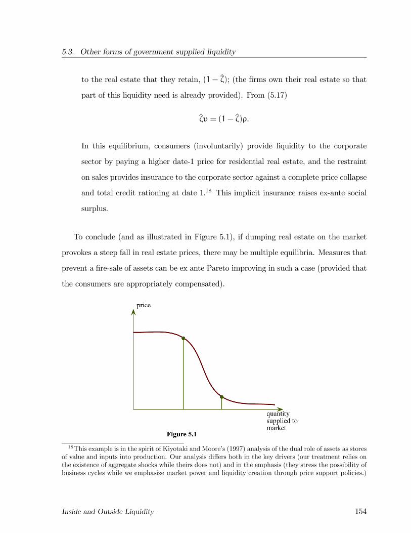
5.3. Other forms of government supplied liquidity
to the real estate that they retain, (1− ζ); (the firms own their real estate so that
part of this liquidity need is already provided). From (5.17)
ζυ = (1− ζ)ρ.
In this equilibrium, consumers (involuntarily) provide liquidity to the corporate
sector by paying a higher date-1 price for residential real estate, and the restraint
on sales provides insurance to the corporate sector against a complete price collapse
and total credit rationing at date 1.18 This implicit insurance raises ex-ante social
surplus.
To conclude (and as illustrated in Figure 5.1), if dumping real estate on the market
provokes a steep fall in real estate prices, there may be multiple equilibria. Measures that
prevent a fire-sale of assets can be ex ante Pareto improving in such a case (provided that
the consumers are appropriately compensated).
18This example is in the spirit of Kiyotaki and Moore’s (1997) analysis of the dual role of assets as stores
of value and inputs into production. Our analysis differs both in the key drivers (our treatment relies on
the existence of aggregate shocks while theirs does not) and in the emphasis (they stress the possibility of
business cycles while we emphasize market power and liquidity creation through price support policies.)
Inside and Outside Liquidity 154
5.3. Other forms of government supplied liquidity
Remark: Allen and Gale (e.g.,1994, 1998) have provided early analyses of fire sales in
the context of the Diamond-Dybvig model of consumer liquidity demand reviewed in
Appendix 2.2. In those papers investors invest in an uncoordinated fashion in liquid
(short-term) assets, that yield a safe return at the intermediate date, and in higher-yield
illiquid (long-term) assets. A fraction of consumers, the “impatients”, want to consume
at the intermediate date; they use the returns on the short-term assets and also resell
their long-term assets. How much these long-term assets fetch in the secondary market
depends on the realized number of consumers who desire to consume early; so there is
aggregate uncertainty. Consumers who desire to consume late use the proceeds of their
short-term assets to purchase the long-term assets not wanted by the consumers who
desire to consume early. The former — the buyers — have limited cash on hand, and so
the asset price decreases when more consumers — the sellers — want to dispose of their
long-term assets in the market. This phenomenon is called “cash-in-the-market pricing”
by Allen and Gale.19
Soft pricing: selling assets to consumers at the intermediate stage.
Finally, we turn to a brief analysis of price stabilization using restricted trade. Assume
that the representative firm invests a fixed amount I at date 0, and faces a random shock
ρ per unit of continuation investment at date 1, where ρ is drawn from the distribution
F(ρ). It can then reinvest i(ρ) ∈ [0, I]. The shock is the same for all firms so there is onlyaggregate uncertainty. Each identical entrepreneur has endowment A ≥ I at date 0 andno endowment thereafter.
The only store of value in the economy is the investment itself, which can be sold to
consumers (liquidated) at date 1 at a market determined price p. When facing a shock
19Allen and Gale then allow intermediaries to pool liquidity, while still offering non-contingent deposit
contracts. The lower the resale price, the more long-term assets the intermediary needs to sell in order to
honour its commitment towards depositors. This, together with the intermediaries’ limited liability, adds
a discontinuity in the resale price of the secondary asset. If the resale price is too low, the intermediary
goes bankrupt and then its entire holdings of long-term assets are dumped on the market, creating a
“crisis”. Related work on fire sales has recently been done by Diamond and Rajan (2009).
Inside and Outside Liquidity 155
5.3. Other forms of government supplied liquidity
ρ > ρ0, firms must sell a fraction of their initial investment if they wish to continue. Let
m be the amount of assets placed on the market at date 1. The consumers’ demand for
assets at date 1 is described by a downward sloping demand curve p(m), which is derived
from the marginal consumer surplus S0(m). The revenue collected by the representative
firm is R(m) ≡ p(m)m. For purposes of illustration, we will focus on the linear case
p(m) = 1−m.
(i) Free market
Provided that the value ρ1 is “large enough” (see below), firms choose to reinvest as
much as they can by selling in the secondary market. Given the state of nature ρ and the
market price p(m), the maximum scale of investment i is given by
i =p(m)I
(ρ− ρ0) + p(m).
In equilibrium we must have
(ρ− ρ0)(I−m) = R(m) = p(m)m.
This equation defines the equilibrium amount of assets put on the market m =m∗(ρ), or
equivalently the continuation investment i∗(ρ), since i∗(ρ) = I −m∗(ρ). In general, the
equilibrium will not be unique; in the linear case there is either one or two equilibria.
Continuing with the investment at date 1 has a positive net present value provided
that ρ1 ≥ p + ρ. For example, with I = 1, we have (ρ − ρ0)(1 −m) = m(1 −m) =⇒m∗(ρ) = ρ−ρ0 (a unique equilibrium). In this case, the net present value will be positive
if ρ1 ≥ 1+ ρ0.
(ii) Price stabilization
Let us now show that a state-contingent cap on sales m can sometimes increase total
surplus, which together with a date-0 transfer from entrepreneurs to consumers results in
a Pareto improvement. To this end, imagine that consumers and entrepreneurs agree at
date 0 on a transfer T ≤ A− I and date-1 policies i(ρ) and m(ρ). Given the consumers’
Inside and Outside Liquidity 156
5.3. Other forms of government supplied liquidity
gross surplus S(m) from acquiring m units of assets at date 1, the optimal insurance
contract solves:
maxT,i(·),m(·)
−T + E[(ρ1 − ρ0)i(ρ)]
subject to
T + E[(ρ0 − ρ)i(ρ) + S(m(ρ))] ≥ U,(ρ− ρ0)i(ρ) ≤ R(m(ρ)), for all ρ,
i(ρ) +m(ρ) ≤ I,I+ T ≤ A.
In this Pareto program, the representative entpreneur’s expected utility is maximized
subject to consumers being guaranteed some level of utility U. The reinvestment i(ρ)
may be constrained either by the date-1 liquidity constraint (ρ − ρ0)i ≤ R(m) or by thetechnological constraint i+m ≤ I.Rather than solve the entire program, we will investigate whether reducing m slightly
by capping sales below the market level can improve welfare. To simplify matters we
assume that the entrepreneur’s endowment A is so large that the shadow value of the
consumers’ budget constraint is 1. In that case, we can substitute the budget constraint
into the objective function to obtain the maximand E[(ρ1−ρ)i(ρ)+S(m(ρ))]. Note thatif the market equilibrium m∗(ρ) lies below the monopoly level (i.e. R0(m∗(ρ)) ≥ 0) it
cannot be improved by capping m, because a decrease in m reduces the revenue R(m)
and, through the liquidity constraint, the reinvestment i. Therefore, we are only interested
in levels of m beyond the monopoly level.
Two cases, depicted in Figure 5.2, need to be considered:
Inside and Outside Liquidity 157
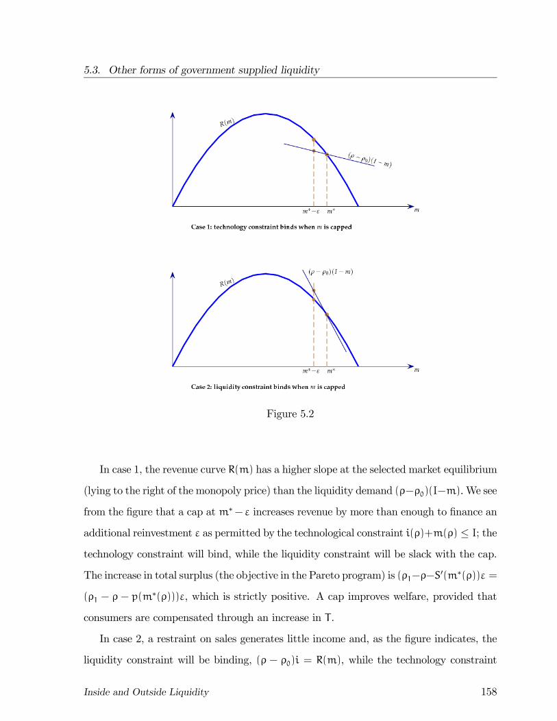
5.3. Other forms of government supplied liquidity
Figure 5.2
In case 1, the revenue curve R(m) has a higher slope at the selected market equilibrium
(lying to the right of the monopoly price) than the liquidity demand (ρ−ρ0)(I−m).We see
from the figure that a cap at m∗−ε increases revenue by more than enough to finance an
additional reinvestment ε as permitted by the technological constraint i(ρ)+m(ρ) ≤ I; thetechnology constraint will bind, while the liquidity constraint will be slack with the cap.
The increase in total surplus (the objective in the Pareto program) is (ρ1−ρ−S0(m∗(ρ))ε =
(ρ1 − ρ − p(m∗(ρ)))ε, which is strictly positive. A cap improves welfare, provided that
consumers are compensated through an increase in T .
In case 2, a restraint on sales generates little income and, as the figure indicates, the
liquidity constraint will be binding, (ρ − ρ0)i = R(m), while the technology constraint
Inside and Outside Liquidity 158
5.4. Concluding remarks
stays slack, i < I−m. This means that some of the initial investment will be completely
wasted. Nonetheless, the cap may generate an increase in surplus. This occurs when
(ρ1 − ρ)di+ pdm =
∙(ρ1 − ρ)
µ−
R0
ρ− ρ0
¶− ρ
¸ε > 0.
For example when I = 1 (and p(m) = 1−m), this condition becomes ρ1 > ρ0+m2
2m−1. Near
the monopoly price, very little extra revenue is generated when m is reduced, implying
that i cannot be increased much and instead most of the reduction in m goes to waste.
In case 2, an equilibrium that is close to the monopoly price cannot be improved upon
using a cap.
We conclude that efforts to stabilize the market price (perhaps with the help of gov-
ernment), by reducing the amount of asset sales when liquidity is scarce, can be beneficial.
Of course, price stabilization is only one instrument to transfer income from consumers
to firms. For policy purposes, the relative merits/inefficiencies of the various instruments
need to be compared, but we have not attempted to do that.
Remark: Lorenzoni (2008) motivates the consumers’ downward sloping demand for second-
hand corporate assets in a different way (consumers are endowed at date 1 with an al-
ternative, decreasing-returns-to-scale storage technology), but this is inconsequential. He
also shows that there is over-borrowing (I is too high).
5.4 Concluding remarks
The main message of this chapter is that the government can play an important role in
supplying and managing liquidity. When there is a wedge between total and pledgeable
income, privately supplied liquidity may not be sufficient for supporting second-best pro-
duction plans. Put differently, optimal risk sharing within the productive sector, when
all contracts have to be backed up claims on real output, may fall short of second-best,
because of a shortage of aggregate liquidity. Consumers, directly or through intermedi-
aries, would be willing to provide insurance that firms want, but there are not enough
Inside and Outside Liquidity 159
5.4. Concluding remarks
claims to back up such promises. We take the view that the government is in a position
to back up such promises because of its unique right to tax. We have shown that granted
this ability, government intervention, especially in rare states of nature where liquidity
is exceptionally short, is warranted. We have also shown that the basic logic behind the
optimal supply of government liquidity follows the logic of state-contingent pricing of the
kind seen in traditional general equilibrium models.
One of the many open issues that deserves serious attention is the optimal channel
for the government to use in distributing liquidity. It is reasonable to conjecture that
banks and related intermediaries are the natural channels to use, because they have the
expertise to know which entrepreneurs are deserving of more liquidity. Another important
issue is what price signals the central bank or the government might use to decide when
and how to intervene. The central bank is in a unique position to signal or certify states of
liquidity shortage by making announcements or more convincingly by acting.20 The YK2
intervention as well as the interventions triggered by the subprime crisis were based on
price signals such as liquidity premia and unusual spreads. It is likely that other signals
could have proved useful, too. Also, the government should be, and seems to be, letting
the shape of the yield curve determine the duration of bond issues. The optimal use of the
yield curve could be approached from the point of view of aggregate liquidity shortages
as well (see Holmström and Tirole, 2001).
We have also hinted at the possibility that liquidity depends in complex ways on the
equilibria in the labour and asset markets. Again, this suggests some scope for govern-
ment intervention. Viewed more broadly, the government can either create some “general
purpose liquidity” in the form of stores of value that any economic agent in the economy
can make use of. Or it can provide more “directed liquidity”, that aims at resolving a
particular source of liquidity shortage. Unemployment insurance makes consumers more
willing to invest their savings in long-term securities, thereby creating more liquidity for
20For a specific proposal, see Caballero and Kuralt (2009).
Inside and Outside Liquidity 160
5.4. Concluding remarks
the corporate sector. Asset price stabilization makes the corporate sector less dependent
on outside stores of value. In a similar vein, the state often targets its provision of liquidity
to the banking sector, that then dispatches the liquidity to the non-financial sector. We
know very little about the optimal structure of liquidity provision, and this is definitely
a key subject for future investigation.
Throughout this chapter, we have assumed that the government ccan costlessly com-
mit to actions, such as state-contingent interventions. We have done so, to highlight
the potential benefits of government interventions. In reality, problems of commitment
are serious and will constrain what types of interventions are worthwhile. The political
economy issues related to government interventions is a large and fruitful area of research.
Inside and Outside Liquidity 161
Chapter 6
Is there still scope for public
liquidity provision when firms have
access to global capital markets?
In this chapter we study an economy with free access to global financial and goods markets.
We have two objectives in mind with this extension. The first is to suggest that the model
we have developed, appropriately extended to an international context, can offer a useful
perspective on worldwide events such as the 1990s financial crises in Thailand and Mexico
and the current concerns about global imbalances. Our second, closely related objective
is to address a conceptual question of great relevance for our study: How can a shortage
of savings/insurance instruments in a small country like Thailand play any significant
role given the enormous depth, scope and liquidity of today’s global financial markets?
Why would Thai companies, banks and the Thai government not be able to meet their
liquidity needs on international financial markets using foreign exchange swaps, dollar or
euro loans and lines of credit and foreign bond and equity investments? Our theory rests
on a shortage of aggregate liquidity within a country. If a national shortage of liquidity
could easily be overcome through international financing, our theory would be of little
relevance.
There is a simple reason why international markets cannot meet a country’s liquidity
needs despite an abundance of international financial instruments for saving and insur-
162
ance. Foreign investments and foreign debts have to be paid with (or be backed up by)
the country’s pledgeable income internationally, namely its net production of tradable
goods. Therefore the amount of foreign liquidity that a country can access — the amount
of international insurance that it can buy — is constrained by the amount of pledgeable
tradable income that it has. Thus, the problem is not that international markets have
limited instruments for transporting wealth from one period to the next or for securing
insurance across states, but rather that the country that seeks insurance may not produce
enough tradable goods to pay for them.
The theory of aggregate liquidity shortages has interesting applications in international
finance. Following Caballero and Krishnamurthy (2001, 2002, 2003a,b), we distinguish
between a country’s international collateral and its domestic collateral. International
collateral consists of claims backed up by tradable goods, while domestic collateral consists
of claims backed up by non-tradable goods.1 Our objective is to indicate, through two
simple examples, how the implications of aggregate liquidity shortages get enriched and
modified when firms have access to international financial markets.
We show that, if international collateral is scarce, the need for domestic collateral and
government intervention remains relevant as in our earlier analysis without international
financial markets, but the prescriptions are somewhat different. We analyze how the
task of liquidity supply is ideally shared between the three providers of liquidity: (i)
the corporate sector; (ii) the domestic government; and (iii) the international financial
markets. We conclude with some thoughts on the role of multilateral organizations such
as the IMF in dealing with national liquidity shortages.
1Domestic consumers will be indifferent between consuming tradable and non-tradable goods. For
this reason, we could alternatively have defined domestic liquidity as the value of all pledgeable goods.
Inside and Outside Liquidity 163
6.1. A model with domestic and international liquidity
6.1 A model with domestic and international liquid-
ity
We extend our basic model to a small open economy facing aggregate shocks that on the
international financial markets can be considered idiosyncratic and therefore are priced
like riskless assets. We are interested in how the corporate sector makes optimal use of
international insurance and how the government supplies and manages liquidity in this
situation, assuming that arbitrarily rich contracts contingent on domestic shocks can be
written.
• Goods and preferences.There are two kinds of goods:
— Tradable goods, which are consumed by foreigners as well as domestic residents.
These goods will at times be called dollar goods or simply dollars.
— Nontradable goods, which only domestic residents consume. These goods are called
peso goods or pesos.
All variables referring to dollars are indexed by a $-sign, while those referring to pesos
are non-indexed.
There are three periods, t = 0, 1, 2. Economic agents only care about the sum of their
consumption at the three dates, and therefore demand a zero expected rate of return on
investments. We further assume, mainly for convenience, that domestic residents view
tradables and nontradables as perfect substitutes. Thus, a foreigner’s utility from the
consumption stream©c$tªt=0,1,2
is2Xt=0
c$t ,
while a domestic resident’s utility from the consumption stream©¡c$t , ct
¢ªt=0,1,2
is
2Xt=0
£c$t + ct
¤.
Inside and Outside Liquidity 164
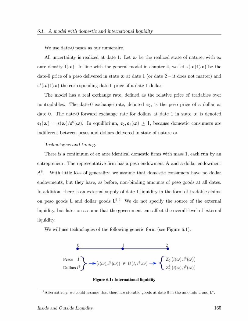
6.1. A model with domestic and international liquidity
We use date-0 pesos as our numeraire.
All uncertainty is realized at date 1. Let ω be the realized state of nature, with ex
ante density f(ω). In line with the general model in chapter 4, we let s(ω)f(ω) be the
date-0 price of a peso delivered in state ω at date 1 (or date 2 — it does not matter) and
s$(ω)f(ω) the corresponding date-0 price of a date-1 dollar.
The model has a real exchange rate, defined as the relative price of tradables over
nontradables. The date-0 exchange rate, denoted e0, is the peso price of a dollar at
date 0. The date-0 forward exchange rate for dollars at date 1 in state ω is denoted
e1(ω) = s(ω)/s$(ω). In equilibrium, e0, e1(ω) ≥ 1, because domestic consumers are
indifferent between pesos and dollars delivered in state of nature ω.
Technologies and timing.
There is a continuum of ex ante identical domestic firms with mass 1, each run by an
entrepreneur. The representative firm has a peso endowment A and a dollar endowment
A$. With little loss of generality, we assume that domestic consumers have no dollar
endowments, but they have, as before, non-binding amounts of peso goods at all dates.
In addition, there is an external supply of date-1 liquidity in the form of tradable claims
on peso goods L and dollar goods L$.2 We do not specify the source of the external
liquidity, but later on assume that the government can affect the overall level of external
liquidity.
We will use technologies of the following generic form (see Figure 6.1).
2Alternatively, we could assume that there are storable goods at date 0 in the amounts L and L∗.
Inside and Outside Liquidity 165

6.1. A model with domestic and international liquidity
Date 0 : Firms invest I, I$.
Date 1 : Conditional on the realized state of nature ω firms make reinvestments
i(ω) and i$(ω). The total cost of reinvestment in state ω is Z(i(ω), i$(ω)) pesos and
Z$(i(ω), i$(ω)) dollars. We use capital letters to distinguish total payoffs from per-unit-
of-scale payoffs. Reinvestments (i(ω), i$(ω)) are constrained by the initial investments
and the state ω, described abstractly at this point by a compact set D(I, I$,ω), that is,
(i(ω), i$(ω)) ∈ D(I, I$,ω).
Date 2 : The pledgeable peso and dollar payoffs Z0(i(ω), i$(ω)) and Z$0(i(ω), i
$(ω))
as well as the total payoff Z1(i(ω), i$(ω)), are realized. We assume the non-pledgeable
private benefit Z1 − Z0 − Z$0 is always strictly positive. Note that we write the total
payoff without a $-sign, because it makes no difference whether private benefits are peso
or dollar goods.
Because international investors only consume tradables, all promises to international
investors have to be backed up by claims on dollar goods. The amount of interna-
tional collateral produced by the corporate sector is Z$0(i(ω), i$(ω)). Since domestic
investors are indifferent between consuming tradables and non-tradable goods the total
amount of collateral available for transactions on the domestic market is Z0(i(ω), i$(ω))+
Z$0(i(ω), i$(ω)), the sum of domestic collateral Z0(i(ω), i
$(ω)) and international collat-
eral Z$0(i(ω), i$(ω)).
The firm’s decision problem.
The representative firm has to decide on the level of initial investments I and I$ and
the date-1 choice (i(ω), i$(ω)). The firm also has to make sure it has enough liquidity to
implement this investment plan. For this purpose the firm buys domestic and international
liquidity `(ω) and `$(ω) at the going prices s(ω)f(ω) and s$(ω)f(ω). These variables
are negative if the firm sells liquidity (i.e. promises net payments to investors). When
buying liquidity the firm takes into account that international liquidity can substitute
Inside and Outside Liquidity 166
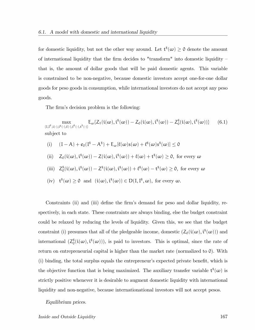
6.1. A model with domestic and international liquidity
for domestic liquidity, but not the other way around. Let t$(ω) ≥ 0 denote the amountof international liquidity that the firm decides to "transform" into domestic liquidity —
that is, the amount of dollar goods that will be paid domestic agents. This variable
is constrained to be non-negative, because domestic investors accept one-for-one dollar
goods for peso goods in consumption, while international investors do not accept any peso
goods.
The firm’s decision problem is the following:
maxI,I$ ,i(·),i$ (·),`(·),`$ (·),t$ (·)
EωZ1(i(ω), i$(ω))− Z0(i(ω), i
$(ω))− Z$0(i(ω), i$(ω)) (6.1)
subject to
(i) (I−A) + e0(I$ −A$) + Eω[`(ω)s(ω) + `
$(ω)s$(ω)] ≤ 0
(ii) Z0(i(ω), i$(ω))− Z(i(ω), i$(ω)) + `(ω) + t$(ω) ≥ 0, for every ω
(iii) Z$0(i(ω), i$(ω))− Z$(i(ω), i$(ω)) + `$(ω)− t$(ω) ≥ 0, for every ω
(iv) t$(ω) ≥ 0 and (i(ω), i$(ω)) ∈ D(I, I$,ω), for every ω.
Constraints (ii) and (iii) define the firm’s demand for peso and dollar liquidity, re-
spectively, in each state. These constraints are always binding, else the budget constraint
could be relaxed by reducing the levels of liquidity. Given this, we see that the budget
constraint (i) presumes that all of the pledgeable income, domestic (Z0(i(ω), i$(ω))) and
international (Z$0(i(ω), i$(ω))), is paid to investors. This is optimal, since the rate of
return on entrepreneurial capital is higher than the market rate (normalized to 0). With
(i) binding, the total surplus equals the entrepreneur’s expected private benefit, which is
the objective function that is being maximized. The auxiliary transfer variable t$(ω) is
strictly positive whenever it is desirable to augment domestic liquidity with international
liquidity and non-negative, because internationational investors will not accept pesos.
Equilibrium prices.
Inside and Outside Liquidity 167
6.1. A model with domestic and international liquidity
The prices for contingent peso liquidity, s(ω) ≥ 1, have to be such that the exogenousdate-1 supply of peso liquidity L(ω) in state ω covers the representative firm’s demand
`(ω):
` (ω) ≤ L(ω), for every ω, with s(ω) = 1, if the constraint is slack. (6.2)
There is no corresponding condition for dollar liquidity, because foreign investors are
not collateral constrained. By assumption, the international markets are deep enough
to back up any dollar pledges that international investors make. Instead, the relevant
constraint is the availability of domestic dollars. Foreign investors need to get paid the
expected dollar return required in international markets (0, because domestic risk is or-
thogonal to world risk). This gives the equilibrium condition for the date-0 exchange rate
e0:
I$ + Eω`$(ω) ≤ A$ + EωL$(ω), with e0 = 1, if the constraint is slack. (6.3)
What about prices s$(ω)? Contingent date-1 dollars must cost the same as date-0
dollars, so
e0 = s$(ω) ≥ 1, for every ω. (6.4)
To see why, recall that the price s$(ω) is the peso price for contingent dollars. Also,
date-1 contingent dollars can be bought at a zero premium in international markets using
dollars. Now, if 1 ≤ e0 < s$(ω), a firm could buy date-0 dollars in the domestic market forthe price e0 and exchange these dollars for contingent dollars in the international market.
This would be cheaper than buying contingent dollars using pesos in the domestic market
eliminating the price premium s$(ω) > e0. In the reverse case — e0 > s$(ω) ≥ 1 —
the arbitrage runs in the opposite direction. A firm could buy contingent dollars in the
domestic market, sell them in the international market in exchange for date-0 dollars that
would cost less than e0. There would be no demand for domestic date-0 dollars to sustain
a price differential.
Inside and Outside Liquidity 168
6.2. All output tradable
Finally, because dollar goods — either consumed or used as collateral — are perfect
substitutes for peso goods, their value has to be at least as high as that of peso goods.
We conclude that
e0 = s$(ω) ≥ s(ω) ≥ 1, for every ω. (6.5)
International investors do not earn any rents. Rents (in addition to the non-pledgeable
income) go to entrepreneurs with pledgeable income in states where liquidity is scarce as
well as to domestic agents who have date-0 dollar endowments.
Rather than analyzing the general model, we highlight its key features with two illus-
trative examples.
6.2 All output tradable
We start with the case where all pledgeable output is tradable, because it provides a useful
benchmark. When all pledgeable output is tradable, international markets can meet the
firms’ liquidity demands at zero cost. Consequently, there is no need for domestic liquidity
supply; the solution is the same as when domestic liquidity is so plentiful that it commands
a zero liquidity premium.
It will not matter in the end, but for now, let us assume that all inputs as well
as the endowment of the representative firm are in peso goods (A$ = I$ = Z$ ≡ 0).
To simplify further, consider our standard constant returns-to-scale technology. Firms
initiate projects at date 0 by choosing an initial investment scale I measured in pesos. At
date 1, an additional amount of pesos ρI is needed to continue the projects at full scale,
where ρ is the liquidity shock, which we assume has a continuous distribution. The date-1
shock ρ represents the stateω, so we will use ρ instead of ω to denote the state of nature.
The date-1 decision concerns the extent of downsizing from I to i. A smaller continuation
scale i(ρ) ≤ I can be chosen by reinvesting Z(ρ) = ρi(ρ). Furthermore Z$ = 0. At date 2,
projects produce no pledgeable peso goods (Z0 = 0), a pledgeable amount of dollar goods
Inside and Outside Liquidity 169
6.2. All output tradable
Z$0 = ρ$0i(ρ) and a private benefit (ρ1 − ρ$0)i(ρ), consumed by the entrepreneur.
Assume tentatively that there is no shortage of liquidity at date 1. This is equivalent
to positing equilibrium prices
e0 = s$(ρ) = s(ρ) = 1. (6.6)
With these prices the representative firm chooses the optimal investment I and the optimal
continuation rule i(ρ) by solving
maxI,i(·)
E[(ρ1 − ρ$0)i(ρ)] (6.7)
subject to
(i) I−A ≤ E[(ρ$0 − ρ)i(ρ)],
(ii) 0 ≤ i(ρ) ≤ I, for all ρ.This is the same program as we analyzed in Section 2. The optimal continuation rule
takes the form i(ρ) = I if ρ ≤ ρ∗ and i = 0 otherwise, where the optimal cut-off level ρ∗
satisfies
ρ$0 < ρ∗ < ρ1. (6.8)
Is there enough liquidity to implement this second-best plan at a zero premium as
posited in (6.6)? The answer is yes. We have assumed that international financial markets
are willing to offer domestic firms insurance at a zero premium up to their pledgeable
dollar income. Since all the firm’s pledgeable income is in dollars and dollars are as
good collateral as pesos, the only constraint on the firm’s access to liquidity is its budget
constraint (6.1)(i). This confirms that (6.6) is indeed an equilibrium.
The simple but important point here is that when all the pledgeable output is in
dollars, there is no role for government supplied domestic liquidity. If a small open
economy has enough export income, international markets can in principle eliminate any
domestic liquidity shortages. This conclusion holds quite generally. It holds for the model
Inside and Outside Liquidity 170
6.3. Tradable and non-tradable outputs
we described in Section 6.1 with the added restriction that pledgeable output is in dollars.
It is also true if firms like to save at date 0, that is, I−A < 0, since savings can be done
on international markets at no cost.
In the example firms choose incomplete insurance (ρ∗ < ρ1), even though interna-
tional investors offer insurance on actuarially fair terms. This is the key implication of
optimal risk management with limited pledgeability: both initial investments and contin-
uation investments will be credit rationed. Placed in an international context, such credit
rationing suggests that a country, even if it could do otherwise, will leave its corporate
sector exposed to extreme liquidity shocks. Put a bit provocatively: financial crises can be
part of an optimal insurance plan even in the most favorable of circumstances (when all
collateral is acceptable to international investors). With our linear specification, output
drops to zero when ρ is above the cutoff ρ∗, making a "crisis" appear very dramatic. It
would look less dramatic with a concave date-1 production function. However, as shown
in Rampini-Viswanathan (2010), if there are decreasing returns to scale at the initial
investment stage, then the amount of insurance bought will depend on entrepeneurial
endowments. If these endowments are small, firms (and the nation) will choose to buy
very little or even no insurance due to the same trade-off that drives our cut-off ρ∗. Poor
countries will have to choose plans that make them prone to crises.
6.3 Tradable and non-tradable outputs
In the previous section, there was no role for government supplied domestic liquidity. We
now show that when a country produces limited amounts of tradable goods so that its
international collateral is scarce, there is a role for government supplied domestic liquidity.
This addresses the important concern we raised earlier that international markets might
resolve a small country’s liquidity problems, because international markets are so deep.
We continue to use a constant-returns-to-scale technology and assume that both the
initial investment and the date-1 (per unit) liquidity shock ρ, are in peso goods. As in the
Inside and Outside Liquidity 171
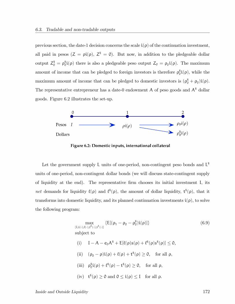
6.3. Tradable and non-tradable outputs
previous section, the date-1 decision concerns the scale i(ρ) of the continuation investment,
all paid in pesos (Z = ρi(ρ), Z$ = 0). But now, in addition to the pledgeable dollar
output Z$0 = ρ$0i(ρ) there is also a pledgeable peso output Z0 = ρ0i(ρ). The maximum
amount of income that can be pledged to foreign investors is therefore ρ$0i(ρ), while the
maximum amount of income that can be pledged to domestic investors is (ρ$0 + ρ0)i(ρ).
The representative entrepreneur has a date-0 endowment A of peso goods and A$ dollar
goods. Figure 6.2 illustrates the set-up.
Let the government supply L units of one-period, non-contingent peso bonds and L$
units of one-period, non-contingent dollar bonds (we will discuss state-contingent supply
of liquidity at the end). The representative firm chooses its initial investment I, its
net demands for liquidity `(ρ) and `$(ρ), the amount of dollar liquidity, t$(ρ), that it
transforms into domestic liquidity, and its planned continuation investments i(ρ), to solve
the following program:
maxI,i(·),`(·),`$ (·),t$ (·)
E[(ρ1 − ρ0 − ρ$0)i(ρ)] (6.9)
subject to
(i) I−A− e0A$ + E[`(ρ)s(ρ) + `$(ρ)s$(ρ)] ≤ 0,
(ii) (ρ0 − ρ)i(ρ) + `(ρ) + t$(ρ) ≥ 0, for all ρ,
(iii) ρ$0i(ρ) + `$(ρ)− t$(ρ) ≥ 0, for all ρ,
(iv) t$(ρ) ≥ 0 and 0 ≤ i(ρ) ≤ I for all ρ.
Inside and Outside Liquidity 172
6.3. Tradable and non-tradable outputs
This program is also a special case of the general program (6.1). Constraints (ii) and
(iii) are the liquidity constraints for pesos and dollars at date 1. These constraints assure
that the demand for peso liquidity `(ρ) and dollar liquidity `$(ρ) are consistent with the
investment plan (I, i(ρ)) and the planned transfer t$(ρ) of dollar liquidity into peso liquid-
ity. These constraints always bind. Negative values for `(ρ) and `$(ρ) imply that the firm
supplies liquidity. The auxiliary variable t$(ρ) is constrained to be non-negative, because
international liquidity cannot be augmented with the help of peso liquidity. Constraint
(i) is the date-0 peso budget constraint. There is no date-0 dollar budget, since dollar
goods can be exchanged into peso goods at date 0 using the date-0 peso prices e0, s$(ρ).
It bears emphasizing that the sole purpose of international liquidity is to alleviate
the domestic shortage of liquidity (or collateral) in this example. To isolate the role
of international markets in supplying stores of value, we have designed the example so
that dollars are not needed for production (there is no international liquidity shock ρ$).
Equilibrium prices are determined by equalizing the supply and demand of domestic
liquidity in each state (see (6.2)) and dollars at date 0 (see (6.3)). In this example, the
equilibrium is characterized by
`(ρ) ≤ L, for every ρ, with equality whenever s(ρ) > 1,
and
E[`$(ρ)] ≤ A$ + L$, with equality whenever e0 > 1.
We know that e0 = s$(ρ) ≥ s(ρ) ≥ 1 for all ρ. The key difference between this example
and the previous one is that prices are not necessarily unity. We can have e0 > 1, because
dollar liquidity can be scarce and we can have s$(ρ) > s(ρ) in some states, because dollars
are potentially more valuable than pesos: they are as good as pesos in consumption, but
unlike peso liquidity, dollar liquidity can be distributed across states through t$(ρ).
Given that all firms are identical, it is easiest to find an equilibrium by solving the
central planner’s problem, which maximizes the representative firm’s utility. In doing so,
Inside and Outside Liquidity 173
6.3. Tradable and non-tradable outputs
we assume, for simplicity, that the available peso liquidity L and the dollar liquidity L$
have been distributed equally across firms by the government. The representative firm’s
program is
maxI,i(·),t$ (·)
E[(ρ1 − ρ0 − ρ$0)i(ρ)] (6.10)
subject to
(i) I−A+ E[(ρ− ρ0)i(ρ)− t$(ρ)] ≤ 0,
(ii) A$ + E[(ρ$0i(ρ) + L$)] ≥ E[t$(ρ)],
(iii) (ρ− ρ0)i(ρ)− t$(ρ) ≤ L, for all ,
(iv) t$(ρ) ≥ 0 and 0 ≤ i(ρ) ≤ I for all ρ.
Constraint (i) is the peso budget constraint. The dollar-peso exchange constraint (ii)
will always hold as an equality. As we have (re)formulated the problem here, the expected
value of the pledgeable dollar income is transferred into the peso budget constraint. The
cost of reinvestments is explicitly accounted for in the budget. The dollar liquidity can be
used to relax the peso liquidity constraints (iii) in an arbitrary state-contingent manner.
This highlights the insurance role of the international investors. They only care about
the expected repayment, not about the states in which repayments are made (see (ii)).
Without access to international markets, there would be no insurance at all across states
ρ, since all firms are hit by the same shock ρ. In each state ρ, the domestic market
would have to make do with the outside domestic liquidity supply L +L$ plus the net
inside liquidity (ρ0 − ρ)i(ρ). For small shocks ρ there would be excess liquidity and for
high shocks ρ there would be a shortage of liquidity. This inefficiency is reduced by the
presence of international investors, who can provide insurance across states.
The extent to which international markets can provide insurance depends on the
amount of pledgeable dollar income that firms generate. We are of course interested
Inside and Outside Liquidity 174

6.3. Tradable and non-tradable outputs
in the case where there is a limited amount of dollar income so that even with insur-
ance through the international market, the liquidity constraint (iii) will be constrained
by available dollars for high enough liquidity shocks ρ. The main questions of interest are
how the foreign and domestic liquidity will optimally be used and how the state prices
will behave.
Let λi, λii and λiii, be non-negative Lagrangian multipliers for the three first con-
straints. The first-order conditions for i(ρ)are:
ρ1 − ρ0 − ρ$0 − (λi + λiii(ρ))(ρ− ρ0) + λiiρ$0 ≥ 0, whenever i(ρ) = I. (6.11)
When 0 < i(ρ) < I, this constraint holds as an equality. The first-order conditions for
t$(ρ) are:
λi − λii + λiii(ρ) = 0, whenever t$(ρ) > 0. (6.12)
When t$(ρ) = 0, the value of additional liquidity is zero, so λiii(ρ) = 0.
From these first-order conditions we can deduce that the solution to the representative
firm’s program has four regions, described formally below and graphically in Figure 6.3.
Inside and Outside Liquidity 175
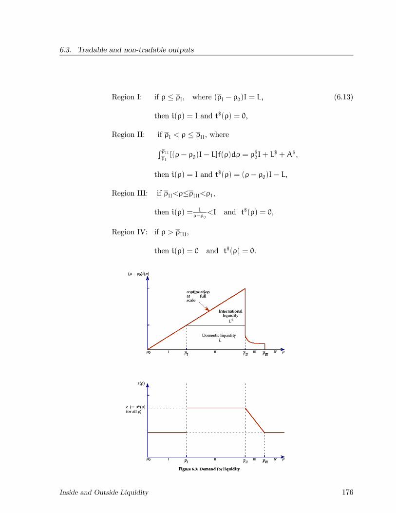
6.3. Tradable and non-tradable outputs
Region I: if ρ ≤ ρI, where (ρI − ρ0)I = L,
then i(ρ) = I and t$(ρ) = 0,
Region II: if ρI < ρ ≤ ρII, whereRρIIρI[(ρ− ρ0)I− L]f(ρ)dρ = ρ$0I+ L
$ +A$,
then i(ρ) = I and t$(ρ) = (ρ− ρ0)I− L,
Region III: if ρII<ρ≤ρIII<ρ1,
then i(ρ) = Lρ−ρ0
<I and t$(ρ) = 0,
Region IV: if ρ > ρIII,
then i(ρ) = 0 and t$(ρ) = 0.
(6.13)
Inside and Outside Liquidity 176
6.3. Tradable and non-tradable outputs
Consider first the top panel in Figure 6.3. In region I, the liquidity shock ρ is so low
that a firm can continue at full scale i(ρ) = I with peso liquidity alone; no dollar liquidity
is needed nor will it be used, since it has a negative shadow price in constraint (ii) (the
shadow price of constraint (iii) is zero and that of (i) is constant, so it is strictly better
to wait until constraint (iii) is binding). This is just saying that there is no point in
wasting precious international liquidity if there is enough domestic liquidity. In region II,
continuation is still at full scale, but requires the addition of dollar liquidity; constraint
(iii) is binding and λiii(ρ) = λiii > 0 is constant, as seen from condition (6.12). As ρ
increases, full scale continuation is possible until the cumulative amount of dollar liquidity
used in region II (the top triangle in the figure) reaches the total amount of available
dollar liquidity. The economic intuition is straightforward: dollars, being scarce, will be
allocated to states in decreasing order of productivity, which means in increasing order
of ρ. In region III the firm reverts back to using only peso liquidity, because all dollar
liquidity has been used up. The scale of continuation investment is now below I and
decreasing in ρ. As in the model without international liquidity, there is credit rationing.
Finally, beyond ρIII < ρ1 it no longer pays to continue.
What about state prices? The prices that will support the centralized solution as an
equilibrium are shown in the lower panel of Figure 6.3.
Start with the price of peso liquidity. In the unconstrained region I, s(ρ) = 1, since
there is an excess of peso liquidity even at full scale i(ρ) = I. In region III, only pesos
are used, but now the continuation investment is below full scale. The price of liquidity
must be such that the firm is persuaded to choose an interior value i(ρ) < I. Since the
marginal value of a peso in region III is declining in ρ, so must its price s(ρ)3. At the left
end of region III we have s(ρII) = s$(ρII); the value of a peso equals the value of a dollar,
since the next best use of a marginal dollar (in state ρII) is to augment pesos in state
3If one goes back to the firm’s program (6.9), one finds that the first-order condition for an interior
solution for i(ρ) requires that s(ρ) = ϕ/(ρ− ρ0), where ϕ is a constant.
Inside and Outside Liquidity 177
6.3. Tradable and non-tradable outputs
ρII + ε. At the right end of region III we have s(ρIII) = 1; since the firm is indifferent
between continuing or not, the marginal peso does not command a premium. Note that
throughout region III, the transfer constraint t$(ρ) ≥ 0 is binding and the shadow priceincreasing. In region II both dollar liquidity and peso liquidity are employed so t$(ρ) > 0.
Since the shadow price on the transfer constraint is zero, both forms of liquidity must
have equal value. In fact,
s(ρ) = s$(ρ) = e0 > 1 throughout region II. (6.14)
The price of liquidity is constant in region II, because a unit of liquidity, regardless of the
state and the currency, will be used in the same manner, namely to increase the date-0
investment I, because the continuation investment equals I in this region. Furthermore,
liquidity prices must equal the exchange rate e0, because exchanging e0 pesos for a dollar
at date-0 and using the proceeds to buy insurance on the international market against
shocks in region II must return the same as buying insurance against these states in the
domestic market.
The date-1 spot exchange rate, defined as the cost of a dollar good in terms of peso
goods, equals 1 in all states, because domestic consumers are equally happy to consume
either good. If e0 > 1, the exchange rate appreciates from date 0 to date 1. This is
an artifact of the three-period model where the need for insurance only occurs in period
0. The (contingent) forward exchange rate e1(ρ) = s(ρ)/s$(ρ) =s(ρ)/e0 will follow the
pattern of s(ρ).
Discussion (public provision of liquidity): We assumed a fixed, non-contingent amount
of government supplied peso and dollar liquidity, L and L$. Referring to the analysis
in the two previous chapters, we can derive some principles for how the government
should optimally participate in the supply of liquidity considering the limited access to
international liquidity. This depends on the government’s objective and the implied cost
of supplying liquidity. The simplest case occurs if consumers have no demand (or a non-
Inside and Outside Liquidity 178
6.3. Tradable and non-tradable outputs
contingent demand) for liquidity and the cost of supplying liquidity (taxing consumers) is
constant in every state. In that case, the government should dispatch a constant amount
of liquidity, just as in the figure, but the cut-off ρII will be determined by the marginal
cost of liquidity supply instead of the exogenously given supply (e.g. it may be optimal
for the government not to supply any liquidity if the marginal cost is high enough). A
less obvious difference is that no outside liquidity will be supplied in region III, which is
eliminated. The reason for this is that partial continuation cannot be optimal other than
at the boundary of region II.4 This is consistent with the use of a state-contingent bond
as discussed in the previous chapter (see also Holmström and Tirole, 1998).
More realistically, the government’s supply function g(L;ω) is increasing and also
varies by state of nature, because the cost of taxation will depend on the consumer demand
for liquidity. The logic behind our analysis in this chapter gives a good indicationn of
how this general case works out. It will still be the case that international liquidity is
most valuable, because it is most flexible. Also, the price of international liquidity will
be constant as a function of the state, else it would be reallocated to its highest value.
Therefore, the price of domestic liquidity will also be constant, except in states where
no international liquidity is used. The amount of domestic liquidity will, however, vary
with the state to reflect the marginal cost ∂g(·;ω)/∂L. The supply of corporate liquiditywould respond to the international price when international liquidity is used and to the
government price of liquidity where such is used. Of course, in the end all of these prices
and decisions are determined jointly in a more complicated equilibrium than we have
studied (i.e. one where the government’s decisions are a part of the equilibrium.)
The main point is that with some of the pledgeable output non-tradable, liquidity
management by the government is again relevant. International investors make insurance
4Suppose we had a region III. There would be partial continuation for all states ρ such that ρII < ρ <
ρIII . Since the cost of government supplied liquidity, q, is constant, it would be more efficient to move
government liquidity from the high-ρ states in region III to the low-ρ states in that region, bringing the
low states to full scale. Consequently, region III cannot exist.
Inside and Outside Liquidity 179
6.4. Conclusion
cheaper, but they cannot provide all of it when international collateral is scarce. Inter-
national liquidity is utilized most efficiently by having international investors supply the
marginal liquidity needed in high demand states. As before, there is capital rationing at
date 1 (a “planned crisis”), but with access to international markets the rationing will be
less severe. Thus, the analysis of the value of domestic outside liquidity in the previous
chapter will be robust to the introduction of international capital markets. This finding
holds as long as some inputs are non-tradable. Had we assumed instead that all inputs at
date 1 were tradable, domestic liquidity supply would be entirely irrelevant. The reason
for this disparity is again that dollars can be substituted for pesos, but not the other way
around.
6.4 Conclusion
This chapter has studied liquidity management when firms have access to international
financial markets and coordinate ex ante on the use of liquidity (second-best insurance).
The main findings are the following:
• International markets will provide adequate insurance if there is sufficient interna-tional collateral. In that case domestic creation of liquidity will be unnecessary.
In general, however, access to international markets does not obviate the need for
domestic creation of liquidity, because the amount of insurance that can be bought
is limited by the amount of international collateral (tradable assets and income).
• Insurance will be incomplete (some states will not be covered) even when there isfull parity between international and domestic liquidity. Optimal risk sharing, with
limited entrepreneurial capital, leaves firms and therefore the country exposed to
the possibility of financial crises. Financial crises are part of an optimal plan even
in the best of circumstances.
Inside and Outside Liquidity 180
6.4. Conclusion
• When international collateral is scarce, the analysis of domestic government policyis similar to that without international markets: the decision to supply liquidity
in a state is determined by comparing state-contingent liquidity premia with the
opportunity cost of providing liquidity in that state. International liquidity will be
used as a last resort, in states where the cost of domestic outside liquidity exceeds
the (domestic) cost of international liquidity. The cost of international liquidity is
strictly positive on the domestic market, whenever domestic dollar output is scarce,
this despite the assumption that international liquidity is supplied at zero cost on
international markets.
Even though this chapter is short and the analysis is presented in the form of simple
examples, it reflects both the richness and the idiosyncratic character of our complete mar-
ket approach. At its core, it is a study of optimal risk sharing under limited pledgeability
of income, reflecting the view that the demand for liquidity is a demand for insuring risks.
Our focus is on how different parties should optimally participate in the supply of risk
sharing. In our analysis there are three parties: the corporate sector, which optimizes
the use of inside liquidity, the government, which intermediates between consumers and
the corporate sector in supplying outside liquidity and finally, the international investors,
who also provide outside liquidity. International insurance is limited by the international
investors’ willingness to accept only tradable goods (or in an alternative interpretation, by
their limited information about and ability to monitor firms in a foreign country). At the
same time, international investors are the most flexible and therefore the most valuable
suppliers of liquidity. By assumption, they do not care about local risks, because they can
diversify away such risk. Both the scarcity of international insurance and the indifference
it displays to local risks, lead it to be used when the domestic, less flexible sources of
insurance, are in short supply or too expensive. The conclusions of this chapter are all
a simple consequence of this general perspective and can be readily extended to include
Inside and Outside Liquidity 181
6.4. Conclusion
shocks to pledgeable and non-pledgeable income as well as liquidation values and income
shocks along the lines discussed in section 4.3.
In reality, international investors do not seem to carry the most expensive domestic
risk as suggested by our point of view. A possible reason for this is that while international
investors have the capacity to insure, they do not have enough information to take on
significant foreign risks. Another reason is that it is hard to write narrowly targeted,
contingent insurance plans ex ante (see section 5.1.2). As a result, international investors
often invest in instruments guaranteed by the government, explicitly or implicitly (e.g.
they invest through domestic banks), or they fund the government directly by buying
government bonds. Even in this case, however, concerns about moral hazard problems —
national governments can take advantage of foreign funding in a variety of ways — limit
the sharing of exceptional risks.5
Unlike private investors, the International Monetary Fund (IMF), has significant mon-
itoring capacity and also leverage over national governments (largely because private in-
vestors would pull out without the IMF). Therefore it can play an important role as a
provider of insurance against sovereign tail risk. During the subprime crisis the IMF has
gone well beyond orthodox interventions (just like central banks) and offered a variety of
liquidity facilities to countries in trouble. These include special drawing rights, contingent
credit lines and systemic liquidity facilities, for instance. Nonetheless, the role played by
the IMF seems rather different from that played by a treasury or a central bank. The
latter, both in practice and in theory (see Chapter 5), act as lenders of last resort, when
there is a shortage of aggregate domestic liquidity. The problem for a country, by contrast,
is not that there are not enough stores of value in the world, but that the country may
have a shortage of tradable goods, which can be pledged to international investors. Also,
5For models of how the level and structure of sovereign and private borrowing affect government
policies and for their implications for capital controls and the policies toward “original sin” features of
borrowing (the issuance of debt claims, that are short-term and denominated in foreign currency), see
e.g., Amador (2008) and Tirole (2003); for an interesting alternative perspective on state opportunism,
see Broner et al (2010).
Inside and Outside Liquidity 182
6.4. Conclusion
the IMF expects to get reimbursed, at least for its largest loans, so it does not provide
liquidity directly.
The IMF would provide liquidity directly only if its claim on the country were de facto
junior to that of public and private lenders and thus involved some substantial risk taking.
Instead, the IMF provides liquidity indirectly, by writing and monitoring the covenants
that will make it more credible that the country reimburses its (sovereign and private)
debts to foreigners. In the parlance of our model, most IMF interventions occur at date 1
when the country has faced a shock to its income or endowment. The covenants increase
the country’s date-2 international collateral at a cost which it can recoup by getting access
to international capital markets, provided that the intervention is credible. And indeed
this is how it should be if a more explicit contract were written between the country and
the international community at date 0.6 The IMF has also tried to venture into “ex ante
monitoring”, which in our model would correspond to writing covenants at date 0. In
1999 it introduced “contingent credit lines”, that were meant to give a country automatic
access to a credit line provided that certain criteria were met; unfortunately, as interesting
as this idea was, no country ever took up those credit lines for fear of being stigmatized
by the signal to the market that it may encounter difficulties in the future.7
We conclude that the cost to monitor what is going on in foreign countries limits the
amount of international risk sharing. The monitoring perspective can also be applied
within a country as we have done in Holmström and Tirole (1997). In that paper, in-
termediaries are better informed than the public about the doings of firms and can more
effectively limit the firms’ ability to engage in moral hazard. To some extent, and as
the recent Eurozone crisis demonstrated, the same applies much more broadly: The will-
6A thorny issue, though, is that the government may not behave in the citizens’ best interests, and
that hardships imposed by covenants — however well justified for the country as a whole at date-0 — may
unduly affect the poor at date 1.
See Tirole (2002) for further discussion of the raison d’être of the IMF.7Accordingly, the IMF in 2009 replaced these contingent credit lines by a new facility, the flexible
credit line: see http://www.imf.org/external/np/sec/pr/2009/pr0985.htm
Inside and Outside Liquidity 183
6.4. Conclusion
ingness to share risk depends on the information and monitoring abilities of all parties
involved. Much of the liquidity is local for this reason. For instance, what goes for good
collateral in one country or one region of a country, may not be worth much in another
country or a distant region within the same country. The approach in this chapter could
be used to study the role of such "local liquidity" more broadly.
Inside and Outside Liquidity 184
Part IV
WASTE OF LIQUIDITY
AND PUBLIC POLICY
185
Chapter 7
Financial muscle and overhoarding of
liquidity
So far our study of aggregate liquidity shortages has assumed that the corporate sector
can make efficient use of the available liquidity in each state of nature at date 1. One
way in which efficient use of liquidity can be assured is to have a complete market of
state-contingent claims on pledgeable income available for trade at date 0. This was
illustrated by the LAPMmodel in Chapter 4. As we discussed earlier, there may be many
institutional solutions for achieving the same outcome, but our model is not rich enough
to distinguish between them. In reality, banks, conglomerates and a variety of other
intermediaries play an important part in trying to allocate state-contingent aggregate
liquidity to its best use. How close these arrangements come to efficiency is an empirical
matter. We view our model of complete contingent contracting as a helpful benchmark
and reference point for such investigations.
In this fourth and final part of the book we depart from the benchmark model and
analyze settings in which firms cannot pool their liquidity to achieve the complete market
outcome. Instead, they have to rely on self-provision of liquidity. In order to meet liq-
uidity shocks that cannot be financed by issuing new claims at date-1 (funding liquidity)
— that is, liquidity shocks that result in a negative net pledgeable income — firms have
to invest in short-term assets that can be liquidated in the date-1 spot market (market
186
liquidity). Firms operate in isolation, without coordinating either the use or the acqui-
sition of liquidity. We also assume that firms cannot hold stakes in each other. These
assumptions are somewhat arbitrary, a problem shared by most models of incomplete
markets. Our choices have been guided by an interest in understanding when investments
in short-term assets will be insufficient and when they will be excessive.
This chapter focuses on reasons why firms may hoard too much liquidity. We will con-
sider two models. In the first model (section 7.1), firms hoard liquidity to put themselves
in a position to compete aggressively for the long-term assets of distressed firms. Our
analysis of such "predatory hoarding" makes two main points: (a) The financial strength
of the potential buyers increases the value of the distressed assets, contributing to liq-
uidity at date 1; (b) uncoordinated purchases of short-term assets at date 0 may result
in excessive hoarding of liquidity. During the subprime crisis (as in earlier crises) banks
have kept large amounts of excess reserves at the central bank (the Fed and the ECB).
This is consistent with the idea that they want to be in a strong position to profit from
fire-sales of distressed assets.1
We will analyze when lack of coordination leads to waste of liquidity and whether the
government can remedy the situation using the following standard instruments:
• Liquidity regulation. The state may mandate minimum or maximum levels of liq-
uidity. For example, some policy proposals following the subprime crisis recommend
a floor on the level of liquidity hoarded by financial institutions. Our analysis sug-
gests that a cap (or tax) on liquidity hoarding may also be warranted, at least when
the anticipation of fire sales makes it likely that financial institutions will stockpile
on liquidity for predatory purposes.
• Public provision of liquidity: As in Chapter 5, the state can change the supply of1Of course, there are other reasons for holding excess reserves. Banks may be concerned about their
own survival in a worsening liquidity squeeze. They may also be waiting for the resolution of uncertainty
that would reduce adverse selection.
Inside and Outside Liquidity 187
7.1. Predatory hoarding of liquidity and fire sales
liquidity. The reason here is not the sharing of aggregate risk, since there are no
aggregate shocks in the model. Instead, the state can influence the way the private
sector manages its liquidity because it can control the price. The public supply of
liquidity has an ambiguous impact if no separate liquidity regulation is in place. As
in Chapter 5, it lowers the cost of liquidity; however it facilitates rent seeking.
The second model (section 7.2) focuses on “precautionary hoarding” of liquidity. In
this framework, firms can use the secondary market to cover their future cash needs; for
instance, they can sell assets that they have hoarded on their balance sheets. If the market
for such assets is marred by asymmetric information, though, it may freeze, depriving the
firms from access to market liquidity. To avoid such a fate, firms may instead hoard
liquidity using safe assets that are not not subject to adverse selection, but the yield on
safe assets, such as Treasury bonds, is low. Interestingly, the tradeoff between investing
in risky assets versus safe assets can lead to multiple equilibria.2 If firms invest mostly in
safe assets, they are less dependent on being able to sell assets in the secondary market.
This creates adverse selection: assets are primarily sold because their owners do not value
them highly and want to get rid of them. In anticipation of such a date-1 "lemons market"
firms indeed want to invest in safe safe assets at date 0.
Conversely, if firms do not expect a market freeze, they prefer to invest in higher
yielding assets that they will sell if they need liquidity. There is less adverse selection,
since asset sales are driven by liquidity shocks rather than shocks to the value of the assets.
This “liquid market" equilibrium dominates the “precautionary hoarding" equilibrium.
Firms would be better off collectively if they could agree not to hoard safe assets.
7.1 Predatory hoarding of liquidity and fire sales
To put our analysis in perspective, it is useful to recall some earlier work on asset re-
deployability. Shleifer and Vishny (1992), building on Williamson (1988), made several
2See Malherbe (2009).
Inside and Outside Liquidity 188
7.1. Predatory hoarding of liquidity and fire sales
insightful observations about the limited ability of distressed firms to resell assets. To
illustrate their reasoning, consider the following parable.
Parable of the farmer and his land : A farmer may have expertise in cultivating a specific
crop, but must borrow cash from a bank in order to purchase the land. Ex post, the
farmer may prove competent or incompetent; or, equivalently, the crop he has expertise
in may turn out to be well adapted to the soil (or in high demand) or ill adapted (in low
demand). If things go poorly, the land, which optimally is pledged as collateral to the
bank, must be resold on the market. One may distinguish three types of sales:
• Alternative use : The land may be transformed by the buyer into, say, a baseballfield. The issue with this type of sale is that the new usage does not correspond
to the best use of the land if keeping it for farming purposes yields a higher social
value.
• Deep-pocket investor : The land is sold to investors with no farming expertise, whohire a farmer to plant and harvest a new crop. This approach has the advantage of
maintaining the land in its best use, but faces an agency cost; and so it creates a
wedge between the total value created and the price that the investors are willing
to pay for the land.
• Specialist : To avoid this agency cost, it would seem more natural to resell the landto another farmer. Prospective buyers in this category however may not have the
resources to buy the land themselves, and if they do not they must borrow from
non-specialists, namely the deep-pocket investors considered in the second type of
sale.
Shleifer and Vishny argue that, when assets must be managed by specialists, the wedge
between the value of assets in specialist hands and the price that can obtained by selling
the assets in the market is particularly high for industries in recession. Specialists tend to
Inside and Outside Liquidity 189
7.1. Predatory hoarding of liquidity and fire sales
be found within the same industry and if that industry is in recession, many of them are
likely to be strapped for cash, pushing the market price below its value in the best use.
This section develops a formal analysis of the three types of sales.
7.1.1 Coordinated investment in liquidity
Consider a continuum of entrepreneurial firms with unit mass.
Firms are identical at date 0. Each has initial wealth A. At date 1, a fraction α of
entrepreneurs is revealed to be competent and a fraction 1−α incompetent. “Intact firms”
in this chapter are firms run by competent entrepreneurs, “distressed firms” are firms run
by incompetent entrepreneurs. No one knows at date 0 which firms will be intact. At
date 1, the entrepreneurs’ types are privately revealed. The fraction α is known at date
0, so there is no aggregate uncertainty.
As before, all agents are risk neutral and indifferent over the timing of consumption,
valuing their consumption stream
c0 + c1 + c2.
Thus, the consumer’s required rate of return must be at least zero.
At date 0 the representative firm can invest in two types of assets:
• Long term (LT) assets: If the firm invests I in LT assets at date 0 and its entrepre-neur is revealed to be competent at date 1, the constant-returns-to-scale technology
of section 3.2 applies: The LT asset delivers nothing at date 1. At date 2 it delivers
total income ρ1I and pledgeable income ρ0I, where
ρ0 < 1 < ρ1.
For simplicity, we assume that no reinvestment is needed at date 1.
If an entrepreneur turns out to be incompetent, the LT asset yields nothing (ρ0 =
ρ1 = 0) under his management. Competent entrepreneurs can manage any number
Inside and Outside Liquidity 190
7.1. Predatory hoarding of liquidity and fire sales
of assets and LT assets may be transferred from incompetent to competent entre-
preneurs in a date 1 spot market. Assets transferred to competent entrepreneurs
yield the same return as the entrepreneurs’ original assets. LT assets may also be
employed in an alternative use (converted to a “baseball field”), with a total return
equal to the pledgeable income ρI where ρ < 1 can exceed or be smaller than ρ0.
An incompetent entrepreneur’s assets will either be converted to the alternative use
or be put under a competent entrepreneur’s management, depending on the spot
market price at date 1.
• Short term (ST) assets: A firm has also access to a storage technology. To obtain `units of goods at date 1, the firm must invest g(`) at date 0 in the ST asset, where
g0(0) = 1 , g0(`) > 1 , and g00(`) > 0 for all ` > 0.
Note that the the firm must pay a higher marginal cost the more it hoards liquidity.
For the purpose of this model, one can think of g(`)− ` as the physical depreciation of
the storage good. But we have an alternative interpretation in mind, in which the firms
in this industry compete with other industries for scarce (inside and outside) liquidity
in an economy in which liquid assets command a premium q − 1, where in equilibrium
q = g0(`).3
Coordinated solution. As a benchmark, consider the second-best case in which, at date 0,
the entrepreneurs can agree among themselves and with investors (by forming a conglom-
erate or through contracting) on the levels of long-term and short—term investments and
on the date-1 policy for redeploying the assets. Because there is no reinvestment need at
date 1 and because liquidity is costly, the optimal coordinated policy is not to invest in
ST assets at all:
`∗ = 0. (7.1)
3For this interpretation q should be taken as exogenous at the firm level.
Inside and Outside Liquidity 191
7.1. Predatory hoarding of liquidity and fire sales
Instead, firms agree in advance that the LT assets of the incompetent entrepreneurs will
be turned over to the competent entrepreneurs. Because firms are identical ex ante and
the entrepreneurs are risk neutral, there is no need for financial payments. In this case,
the optimal investment in LT assets, I∗, is given by the usual budget constraint equating
investors’ outlays with the pledgeable income:
I∗ −A = ρ0I∗,
or
I∗ =A
1− ρ0.
7.1.2 Self-provision of liquidity and the market for
distressed assets
Assume now that, at date 0, each firm selects the pair (I, `) independently, without
coordinating its plan with the other firms.4 At date 1 a spot market for assets opens, in
which the entrepreneurs can sell (if they are incompetent) or buy (if they are competent)
long-term assets. The price in the spot market is denoted p. Because a distressed firm
can choose to put its assets in the alternative use, the date-1 price must satisfy p ≥ ρ. If
p > ρ, all the distressed assets are sold in the spot market; if p = ρ some of the distressed
assets may go into the alternative use. In either case the distressed firm will earn pI at
date 1 from its LT investment. The model thus focuses on local liquidity in the sense that
a limited set of players has the knowledge necessary to manage the assets or to buy the
securities. Furthermore, this set is financially constrained.
Intact firms have two potential sources of funds for purchasing distressed assets. They
can sell their short-term assets ` and they can issue new, senior securities at date 1.5 By
4Recall that we also assume that a firm cannot own shares of the other firms.5A distressed firm has no incentive to issue new shares to buy more assets, since the incompetent
entrepreneurs obtain no private value from selling assets or putting assets into the alternative use. In
contrast, permitting dilution by intact firms is valuable from an ex ante point of view, since it is a
cheaper form of liquidity than buying short-term assets. Contingent transfers from investors to firms
would of course also be cheaper than using short-term assets. Such transfers are ruled out as part of the
assumption that firms cannot coordinate the use of liquidity.
Inside and Outside Liquidity 192

7.1. Predatory hoarding of liquidity and fire sales
fully diluting the initial shareholders, an intact firm can raise ρ0(I + j) at date 1, where
I is the initial investment and j is the amount of assets purchased in the spot market.
Together with the ST assets, the new issue has to cover the purchase of new assets, so
the firm’s investment plan has to satisfy the following date-1 liquidity constraint:
pj ≤ ρ0(I+ j) + `. (7.2)
The firm’s investment plan also has to satisfy the following date-0 budget constraint:
I−A+ g(`) ≤ α [ρ0(I+ j) + `− pj] + (1− α) [`+ pI] (7.3)
On the left-hand side are the costs of investments in LT and ST projects. On the right-
hand side are the date-1 net returns. An intact firm will spend pj of its pledgable income
on buying assets. A distressed firm will pay out to investors the returns from its ST assets
plus what it gets by selling the LT assets in the date-1 spot market (or, alternatively, the
returns it gets from putting the LT assets into the alternative use). When the liquidity
constraint (7.2) binds, the first term on the right-hand side of (7.3) is zero. In that case,
initial investors will only cash in on the liquidation of the distressed firms.
It may seem surprising that investors get something only when bad news is received.
In other models of liquidity demand, such as the one considered in the next chapter, bad
news means that more money must be injected in order to avoid downsizing or closure;
in this case, investors provide funding liquidity by agreeing in advance to let their stakes
be diluted and market liquidity by letting the firm’s ST assets be sold. Good news (no
liquidity shock), in these models, make entrepreneurs and investors both better off. Here,
by contrast, good news means an opportunity to purchase distressed assets, which creates
a liquidity need. Funding liquidity and market liquidity are both employed in the good
state, which ex post is beneficial to the entrepreneur, but not to the investors.
For any given price p the representative firm will choose I, j, ` to maximize expected
net utility:
U = α [ρ1(I+ j)− pj] + (1− α)pI− I− [g(`)− `] , (7.4)
Inside and Outside Liquidity 193
7.1. Predatory hoarding of liquidity and fire sales
subject to the the liquidity constraint (7.2) and the budget constraint (7.3).6
An equilibrium in the date 1 spot market obtains when the demand for assets does
not exceed the supply
αj ≤ (1− α)I (7.5)
and p = ρ if the inequality is strict.
It follows immediately from the firm’s maximization problem that
p > ρ0. (7.6)
Suppose, to the contrary, that p ≤ ρ0. The firm could then purchase boundless amounts
of assets j; neither the liquidity constraint nor the budget constraint would constrain it.
Therefore, the purchase of date-1 assets would be self-financing and entrepreneurial rents
could be increased without bounds. This is inconsistent with equilibrium.
Note also that since p ≥ ρ, the option to put distressed assets into the alternative use
is relevant only if
ρ > ρ0. (7.7)
Otherwise the purchase of distressed assets would be self-financing. We will assume that
(7.7) holds for now.
Next we argue that p must satisfy7
p ≤ 1. (7.8)
To see why, consider the following two investment options:
(i) at date 1, the firm buys an extra unit of distressed assets on the spot market at price
6Alternatively (from (7.3)):
U = α(ρ1 − ρ0)(I+ j)−A.
7At first, one may think that ρ1 is the upper bound for p, because that is the social value of an
extra unit of the asset in the hands of a competent entrepreneur. However, this reasoning overlooks the
alternative ways in which a firm can procure an asset for use at date 1.
Inside and Outside Liquidity 194
7.1. Predatory hoarding of liquidity and fire sales
p;
(ii) at date 0 the firm increases its investment I by one unit.
Let us ignore for the moment the firm’s liquidity constraint and consider maximizing
the firm’s NPV subject only to the budget constraint (7.3). Letting λ > 0 be the La-
grange multiplier for the budget constraint, we have the following first-order conditions
for choosing interior values of I and j.
αρ1 + (1− α)p− 1− λ[1− αρ0 − (1− α)p] = 0, for I (FOC-I)
(ρ1 − p)− λ(p− ρ0) = 0, for j (FOC-j)
The first-order condition (FOC-I) is increasing in p while (FOC-j) is decreasing in p.
At p = 1 the two are equal. Since it is cheaper to buy date-1 assets through the spot
market if p < 1 but not if p > 1, and because reintroducing the liquidity constraint can
only work against buying assets through the date-1 spot market, the spot market can be
in equilibrium only if p ≤ 1. Note that this argument rests on the whole plan I, j, `
being agreed on between the investors and the firm. 8
With these preliminaries, we turn to discuss equilibrium outcomes. Figure 7.1 de-
scribes the outcome when ρ > ρ0. The spot market price p increases monotonically with
the fraction α of intact firms, staying within the bounds ρ and 1. There are three possible
regimes or regions of α. Let us look at the conditions under which each region applies,
considering them in reverse order.
8If the intact firms could bid for the date-1 assets by diluting shareholders at will, their purchasing
power in Region III of figure 7.1, would exceed the supply at p = 1 even without any investments in
short-term assets. This would force the price up.
Inside and Outside Liquidity 195
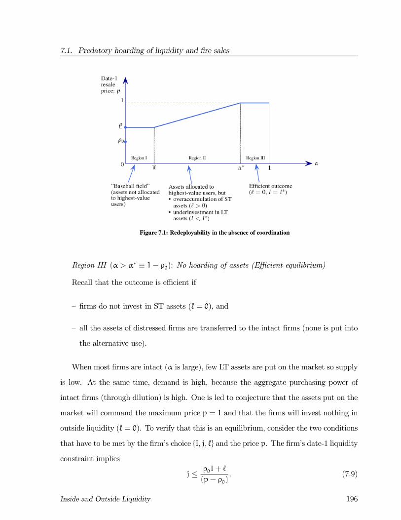
7.1. Predatory hoarding of liquidity and fire sales
Region III (α > α∗ ≡ 1− ρ0): No hoarding of assets (Efficient equilibrium)
Recall that the outcome is efficient if
— firms do not invest in ST assets (` = 0), and
— all the assets of distressed firms are transferred to the intact firms (none is put into
the alternative use).
When most firms are intact (α is large), few LT assets are put on the market so supply
is low. At the same time, demand is high, because the aggregate purchasing power of
intact firms (through dilution) is high. One is led to conjecture that the assets put on the
market will command the maximum price p = 1 and that the firms will invest nothing in
outside liquidity (` = 0). To verify that this is an equilibrium, consider the two conditions
that have to be met by the firm’s choice I, j, ` and the price p. The firm’s date-1 liquidity
constraint implies
j ≤ ρ0I+ `
(p− ρ0). (7.9)
Inside and Outside Liquidity 196
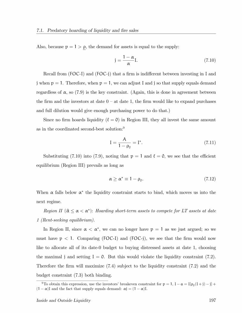
7.1. Predatory hoarding of liquidity and fire sales
Also, because p = 1 > ρ, the demand for assets is equal to the supply:
j =1− α
αI. (7.10)
Recall from (FOC-I) and (FOC-j) that a firm is indifferent between investing in I and
j when p = 1. Therefore, when p = 1, we can adjust I and j so that supply equals demand
regardless of α, so (7.9) is the key constraint. (Again, this is done in agreement between
the firm and the investors at date 0 — at date 1, the firm would like to expand purchases
and full dilution would give enough purchasing power to do that.)
Since no firm hoards liquidity (` = 0) in Region III, they all invest the same amount
as in the coordinated second-best solution:9
I =A
1− ρ0= I∗. (7.11)
Substituting (7.10) into (7.9), noting that p = 1 and ` = 0, we see that the efficient
equilibrium (Region III) prevails as long as
α ≥ α∗ ≡ 1− ρ0. (7.12)
When α falls below α∗ the liquidity constraint starts to bind, which moves us into the
next regime.
Region II (α ≤ α < α∗): Hoarding short-term assets to compete for LT assets at date
1 (Rent-seeking equilibrium).
In Region II, since α < α∗, we can no longer have p = 1 as we just argued; so we
must have p < 1. Comparing (FOC-I) and (FOC-j), we see that the firm would now
like to allocate all of its date-0 budget to buying distressed assets at date 1, choosing
the maximal j and setting I = 0. But this would violate the liquidity constraint (7.2).
Therefore the firm will maximize (7.4) subject to the liquidity constraint (7.2) and the
budget constraint (7.3) both binding.
9To obtain this expression, use the investors’ breakeven constraint for p = 1, I− a = I[ρ0(I+ j)− j] +
(1− α)I and the fact that supply equals demand: αj = (1− α)I.
Inside and Outside Liquidity 197
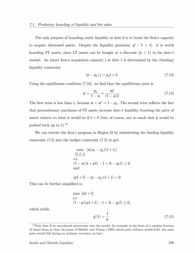
7.1. Predatory hoarding of liquidity and fire sales
The only purpose of hoarding costly liquidity at date 0 is to boost the firm’s capacity
to acquire distressed assets. Despite the liquidity premium, g0 − 1 > 0, it is worth
hoarding ST assets, since LT assets can be bought at a discount (p < 1) in the date-1
market. An intact firm’s acquisition capacity j at date 1 is determined by the (binding)
liquidity constraint
(p− ρ0) j = ρ0I+ `. (7.13)
Using the equilibrium condition (7.10), we find that the equilibrium price is
p =ρ01− α
+α`
(1− α)I. (7.14)
The first term is less than 1, because α < α∗ = 1− ρ0. The second term reflects the fact
that precautionary purchases of ST assets increase date-1 liquidity, boosting the price of
assets relative to what it would be if ` = 0 (but, of course, not so much that p would be
pushed back up to 1).10
We can rewrite the firm’s program in Region II by substituting the binding liquidity
constraint (7.2) into the budget constraint (7.3) to get:
max
I, `, j
α(ρ1 − ρ0)(I+ j)
s.t.
(1− α)(`+ pI)− I+A− g(`) ≥ 0and
[pI+ `]− (p− ρ0)(I+ j) = 0.
This can be further simplified to
max [pI+ `]
s.t.
(1− α)(pI+ `)− I+A− g(`) ≥ 0,which yields
g0(`) =1
p. (7.15)
10Note that if we introduced uncertainty into the model, for example in the form of a random fraction
of intact firms α, then the point of Shleifer and Vishny (1992) about price softness would hold: the asset
price would fall during an industry recession (α low).
Inside and Outside Liquidity 198

7.1. Predatory hoarding of liquidity and fire sales
It follows that ` > 0. In Region II, entrepreneurs engage in wasteful competition for
entrepreneurial rents by acquiring positive amounts of short-term assets. As we will see,
this inefficiency can be reduced by discouraging liquidity hoarding.
A firm’s maximum scale of investment, given that it purchases liquidity `, is given
by the budget constraint (7.3). Substituting expression (7.14) for p into the budget
constraint, we see that a firm invests in equilibrium
I =A− [g(`)− `]
1− ρ0< I∗ . (7.16)
The inequality follows from ` > 0. When the fraction of distressed firms is large (low
α) the date-1 resale market is awash with assets. The price p falls when α falls while
firms respond by increasing ` and reducing I (buying assets in the spot market becomes
increasingly attractive). To see this, suppose p at some α were to (weakly) decrease with
α. Then (7.15) implies that ` would (weakly) increase with α. From (7.16) I decreases
with `, so `/I would (weakly) increase, which would contradict (7.14). Therefore, p must
be increasing in α in Region II.
For some α > 0, determined by equations (7.13) through (7.16) and the firm’s first-
order condition for choosing I, the price eventually hits its lower bound:11
p = ρ > ρ0.
Region I (α < α): Employing some assets in the alternative use (Second-best equilib-
rium).
For values α < α, a fraction of distressed assets are converted to the alternative use.
The situation is somewhat similar to the basic model considered in Chapter 3 in which
(intact) consumers prefer to consume rather than supply liquidity to firms. The reason
why assets are inefficiently employed here is the same: there is a wedge between pledgeable
and total income.
11At the lower bound, we must have ` > 0 or else (7.13) would not hold for p = ρ.
Inside and Outside Liquidity 199
7.1. Predatory hoarding of liquidity and fire sales
We summarize the analysis of this section in:
Proposition 7.1. Suppose that the assets of distressed firms are either sold to intact
firms or converted to an inferior alternative use at value ρ; and that firms procure their
liquidity independently of each other by obtaining the right to issue new claims on their
long term assets at date 1 and by investing in costly short term assets at date 0.
If ρ > ρ0, then the price p at which LT assets are traded at date 1 is increasing in α.
Furthermore, there exist thresholds α∗ and α, 1 > α∗ > α ≥ 0, such thata) if α ≥ α∗, the outcome is second-best efficient and p = 1;
b) if α ≤ α < α∗, firms hoard excess liquidity ( ` > 0) and p < 1; when α decreases, `
increases and p and I decrease.
c) if α < α, firms hoard excess liquidity ( ` > 0) and p = ρ, implying that some fraction
of LT assets will be put into the (inferior) alternative use.
If ρ ≤ ρ0, assets are never placed in the alternative use ( α = 0), but parts (a) and
(b) hold as stated.
If we interpret a lower α as reflecting a worse economic outlook, then the fact that
the date-1 spot price p increases with α implies that there is more hoarding of liquidity
when entrepreneurs become more concerned about the risk of distress and potentially also
when they anticipate a less efficient use of LT assets12
7.1.3 Policy implications
In the following, we ignore Region III (α ≥ α∗) since the uncoordinated solution in this
case coincides with the coordinated (efficient) solution. For the other regions we study
government interventions, for different values of α, keeping in mind that the value of α is
fixed and known to the government at the time it decides on any intervention.
12This property is obtained from the first-order conditions with respect to `, I and j in Region II. In
Region I, set p =ρ and use (7.14) and (7.16).
Inside and Outside Liquidity 200
7.1. Predatory hoarding of liquidity and fire sales
A. Liquidity regulation: imposing a liquidity cap (or taxing liquidity)?13
• Consider first Region II (bα ≤ α < α∗). In this region all firms invest in liquidity and
the intact firms buy all the long-term assets of the distressed firms at date 1. The ex
post allocation is efficient and the deadweight loss stems solely from liquidity hoarding.
Furthermore, even without purchasing any liquidity, intacts can still buy all the long-term
assets on sale, since the spot price will drop accordingly (until it hits its lower bound).
This suggests that a liquidity cap of 0 would be an optimal intervention that would
eliminate rent-seeking without affecting the efficient transfer of assets.
To check this, note that (using (7.10) and (7.14)) the entrepreneur’s net expected
utility in this region is
U = ρ1I− I− [g(`)− `].
Using (7.14), the firm’s budget constraint (7.3) can be expressed as
I−A+ [g(`)− `] ≤ ρ0I.
Because g(`) − ` > 0 is increasing in `, hoarding more liquidity reduces welfare both
directly, and indirectly through the reduction in the investment level that investors are
willing to grant. Thus as long as the LT asset is efficiently reallocated ex post, it is optimal
to cap the use of liquidity as much as possible.
Let us imagine that the government bans liquidity hoarding altogether and sets ` = 0.
For which α values would intacts still be able to buy all the assets of the distressed? In
Region III of figure 7.1, firms privately choose ` = 0, so the government cap has no effect.
When α goes below α∗, firms would like to buy liquidity, but with the government cap
they cannot. As a consequence, their purchasing power in the date-1 market is reduced
and the spot price is smaller than without government intervention as indicated in figure
13A steep tax on excess hoarding, starting at the level of the cap, achieves the same outcome as a cap.
By contrast, an uncompensated tax on hoarding reduces entrepreneurial wealth.
Inside and Outside Liquidity 201
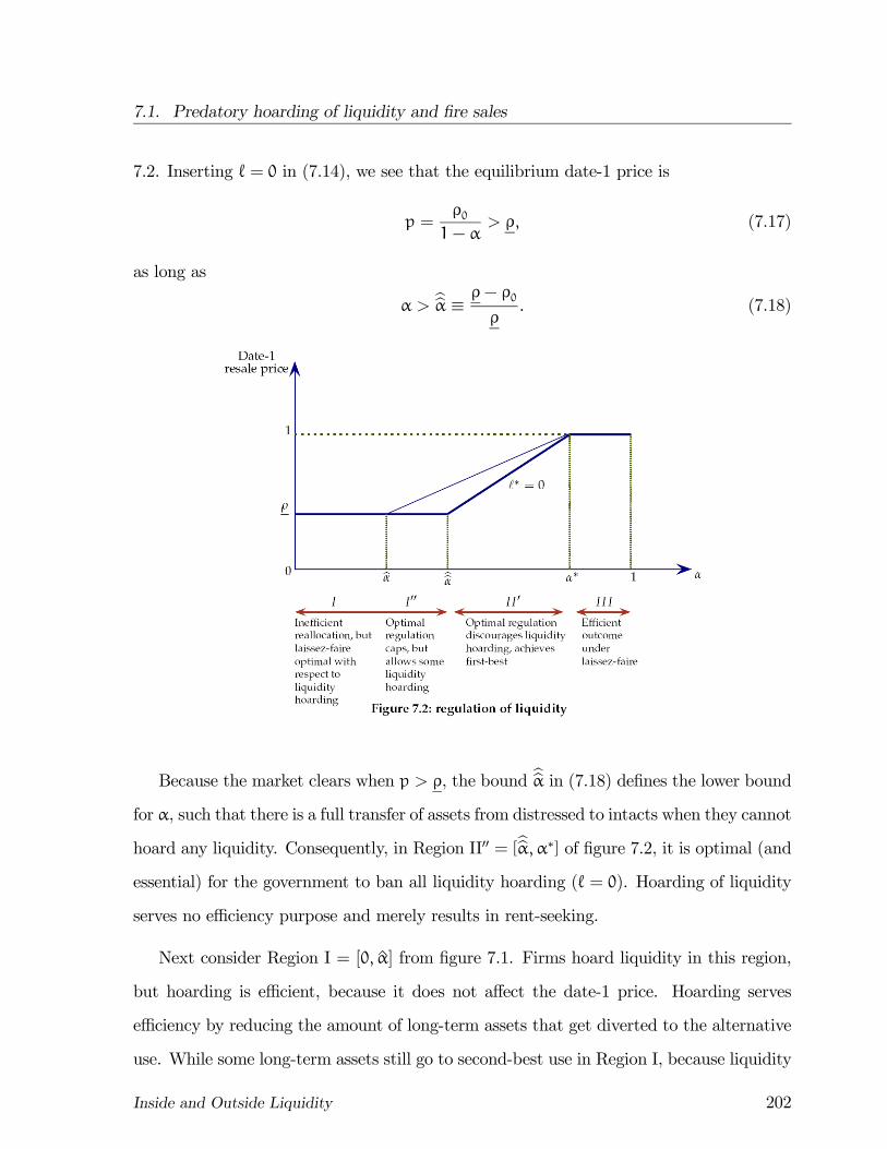
7.1. Predatory hoarding of liquidity and fire sales
7.2. Inserting ` = 0 in (7.14), we see that the equilibrium date-1 price is
p =ρ01− α
> ρ, (7.17)
as long as
α > bbα ≡ ρ− ρ0
ρ. (7.18)
Because the market clears when p > ρ, the bound bbα in (7.18) defines the lower boundfor α, such that there is a full transfer of assets from distressed to intacts when they cannot
hoard any liquidity. Consequently, in Region II00 = [bbα,α∗] of figure 7.2, it is optimal (andessential) for the government to ban all liquidity hoarding (` = 0). Hoarding of liquidity
serves no efficiency purpose and merely results in rent-seeking.
Next consider Region I = [0, α] from figure 7.1. Firms hoard liquidity in this region,
but hoarding is efficient, because it does not affect the date-1 price. Hoarding serves
efficiency by reducing the amount of long-term assets that get diverted to the alternative
use. While some long-term assets still go to second-best use in Region I, because liquidity
Inside and Outside Liquidity 202
7.1. Predatory hoarding of liquidity and fire sales
hoarding is increasingly costly, the government cannot improve on the situation (other
than reducing the cost of liquidity provision — see below). Formally, this can be seen by
checking that in Region I, the government’s optimal program coincides with each firm’s.
(This is left to the reader).
Finally, consider Region I00 = [α, bbα]. Note first that we must have α < bbα, becausepreventing firms from hoarding liquidity reduces their purchasing power in the date-
1 market. Hence the date-1 price will be uniformly lower with than without liquidity
hoarding. However, if the government sets ` = 0, the long-term assets cannot all be
transferred to the intacts and some will go to the alternative use. Below we will show
that it is in the government’s interest to allow some hoarding of liquidity. Indeed, as
long as hoarding does not raise the price in the date-1 market above p = ρ, hoarding of
liquidity will merely improve the transfer of assets from distressed to intacts. If the price
rises above ρ, however, we know that all assets are transferred and some of the liquidity is
used for rent-seeking. Hence, the government’s optimal policy is to allow enough hoarding
of liquidity to permit full transfer of assets without letting the price rise above ρ.
Let
w(`, I) ≡ (1− α)I− αj = (1− α)I−α(ρ0I+ `)
ρ− ρ0
denote the amount of LT assets placed in alternative use (with w = 0 and ` = 0 at
α = bbα). Using the fact that (1− α)ρ > ρ0 in this region, one has
∂w
∂`< 0 and 1 >
∂w
∂I> 0.
Welfare can be written as a function of the two forms of inefficiency, the waste of LT
assets ex post and the inefficient build-up of liquidity ex ante:
U = [ρ1I− I]− [ρ1 − ρ]w(`, I)− [g(`)− `]. (7.19)
The social planner’s budget constraint is:
I−A+ [g(`)− `] ≤ ρ0I+ (ρ− ρ0)w(`, I). (7.20)
Inside and Outside Liquidity 203
7.1. Predatory hoarding of liquidity and fire sales
Sustituting this budget constraint into (7.19) welfare can be written:
U = (ρ1 − ρ0)[I−w(`, I)].
Ignoring the constraint w ≥ 0 for the moment, and substituing out w(`, I) from U
and the budget constraint (7.20), the social planner’s problem can be stated as:
max
I, `
¯α
ρ− ρ0(ρI+ `)
°s.t.
I = [A− g(`) + (1− α)`]/[1− (1− α)ρ].
The solution to this program is given by
g0(`) =1
ρ.
Defining `(p) by g0(`(p)) = 1/p, and rewriting the waste as a function of ` after sub-
stituting for I from the budget constraint, bw(`,α) ≡ w³`,A−g(`)+(1−α)`
1−(1−α)ρ
´, a decreasing
function of `, one has bw(`(p(α)),α) = 0 for α ∈ [bα, bbα], and p(α) > ρ in that range.
Hence bw(`(ρ),α) < 0, which violates the constraint w ≥ 0. Hence at the optimumw = 0.
As we announced, the regulator caps ` at the level that just prevents wasting assets by
converting them to the alternative use.
B. Public provision of liquidity
We next investigate whether the state can improve welfare by increasing availabile
stores of value. We only consider the impact of a marginal increase δ` in the supply per
entrepreneur. Assume that the cost of taxation for the consumers at date 1 is (1+ λ0)δ`
and that the state at date 0 charges each entrepreneur q0 = (1 + λ0)δ`. This keeps the
welfare of the consumers constant, provided that the corporate tax is transferred to them.
Inside and Outside Liquidity 204
7.1. Predatory hoarding of liquidity and fire sales
To make things interesting, we assume that (1 + λ0) is smaller than the marginal cost
of private liquidity creation, g0(`), in the uncoordinated, laissez-faire equilibrium studied
above (otherwise there would be no demand for public liquidity). Finally, we assume that
there is no direct regulation of liquidity.
• Consider first Region I in which the LT asset is partly put into the alternative use
(α < bα). An increase in the public supply of liquidity shifts the cost function downwardsbg(`) = ±
g(`) if g0(`) ≤ 1+ λ0
g(`− δ`) + (1+ λ0)δ` if g0(`− δ`) ≥ 1+ λ0.
The cost function bg(`) is uniformly lower as δ is increased and therefore raises the objectivefunction in the social program above. Public supply of liquidity is (at the margin) welfare-
enhancing.
• In Region II (bα ≤ α < α∗), an increase in the supply of public liquidity has two
opposing effects. As in Region I, it reduces the cost of accumulating liquidity; but it also
encourages rent seeking. Either effect may dominate as seen from the following two cases:
• (i) Suppose that g(`) = q` for ` ≤ ` and +∞ for ` > ` (where q > 1 + λ0),
and that, in equilibrium without public liquidity, ` = `. Adding δ` of public
liquidity increases the deadweight loss from (q− 1)` to (q− 1)`+ λ0δ`. Thus
public liquidity reduces welfare.
(ii) Suppose that g(`) = q`, with q > 1+λ0.14 Now the marginal cost of liquidity,
and therefore the choice of `, is unchanged by additional public liquidity. The
deadweight loss is reduced from (q− 1)` to (q− 1)(`− δ`) + λ0δ` < (q− 1)`,
so public liquidity raises welfare in this case.
Proposition 7.2. (i) In Region I 0 some of the LT assets are wastefully redeployed in
the alternative use, but firms hoard an optimal amount of liquidity, assuming that any
14This violates our assumption that g0(0) = 1, but is inconsequential for our argument.
Inside and Outside Liquidity 205

7.1. Predatory hoarding of liquidity and fire sales
reallocation of liquidity must be voluntary. Suppressing liquidity reduces welfare because it
increases the volume of assets that are turned to the alternative use. By contrast, adding
publicly provided liquidity is welfare enhancing.
(ii) In Region II 0, firms hoard excess liquidity under laissez-faire, but LT assets are properly
reallocated ex post. The tightest possible constraint on liquidity hoarding maximizes wel-
fare. As a potential alternative to regulation, public provision of liquidity has an ambiguous
impact: it reduces the firms’ cost of hoarding liquidity, but it facilitates rent seeking.
We can summarize these results more succintly as follows
• A cap on liquidity hoarding increases welfare as long as assets are reallocated effi-ciently with the cap.
• Firms choose the efficient level of liquidity whenever some of the assets are put intoalternative use.
Remark: Let us return to the observation discussed in the introduction, that many banks
accumulated large amounts of reserves at the Fed and the ECB, possibly to take advantage
of future fire sales, at the same time as other financial institutions and firms were in dire
need of liquidity. In response to a near-zero federal funds rate, the Fed decided to raise
the interest rate on bank reserves deposited at the central bank. This is the opposite of
a policy that would encourage liquidity-rich institutions to invest their extra liquidity in
the private sector. The welfare analysis in this section (regarding the benefits of a cap
and the provision of liquidity) suggests that the Fed’s policy may have been unwise.15
15The Fed’s argument for paying interest on reserves was that this gave the Fed control of an interest
rate that influenced credit. The Federal Funds rate had lost that role in the near-zero environment.
Inside and Outside Liquidity 206
7.2. Precautionary hoarding in anticipation of a market freeze
7.2 Precautionary hoarding in anticipation of a mar-
ket freeze
Drawing on Malherbe (2009), this section studies a model where there may be asym-
metric information about the value of assets at date 1. Under asymmetric information
resale markets may break down as buyers become concerned that lemons are offered for
sale (Akerlof 1970). On the other hand, if buyers know that firms face liquidity shocks
unrelated to the quality of their assets, and that firms do not have insurance against such
shocks, buyers will be less concerned about lemons and date-1 markets will be liquid. Ex-
pecting that the secondary market will be liquid, firms do not need to self-insure as much.
The reason that assets are sold in the date-1 market will then be mostly due to liquidity
shocks, rather than idiosyncratic shocks to the firm’s asset. The fraction of lemons will
be low, confirming the expectation that markets are liquid.
An analogy may be useful here. Students who are moving abroad and selling the car
or the furniture make it clear that they are moving abroad. Similarly, people selling their
house would be inclined to reveal that they are moving out of town or that they move
for life-cycle reasons that make their current house too small or too large. Sellers try to
alleviate adverse selection by disclosing a legitimate reason for selling. A similar effect
operates here as the sellers would want buyers to believe that they are selling an asset,
because of a fragile balance sheet rather than for opportunistic reasons.
To illustrate how adverse selection affects the hoarding of liquidity, we consider the
following model.
Timing and actors. There are three periods, t = 0, 1, 2, and a continuum of firms.
Investment opportunity: At date 1, each firm will have a new (fixed sized) investment
opportunity that, if undertaken, will deliver ρ1 at date 2. To simplify notation, we assume
that none of this value is pledgeable (ρ0 = 0); this is inconsequential for the points we
want to make. With probability α, the investment costs zero and with probability 1− α
Inside and Outside Liquidity 207
7.2. Precautionary hoarding in anticipation of a market freeze
it costs I. There are idiosyncratic liquidity shocks, but no aggregate uncertainty. We note
that investment I could alternatively be interpreted as a reinvestment on a project that
started at date 0, in line with our earlier analyses.
Tradable legacy asset: Each firm owns a legacy asset that will deliver θ at date 2. The
value θ is drawn from a cumulative distribution function F(θ) with support [0, ρ1] and
mean θ.16 The value of the legacy asset is independent of the cost of investment. No one
knows the true value of θ at date 0. At date 1, the firm will have an opportunity to sell
its legacy asset, knowing its true value, while the market will remain uninformed. Later,
we will show that the conclusions are unchanged if a firm knows its θ and can sell the
asset at date 0.
Assumption 1 Without private information, the firm could finance the date-1 project in
all states of nature by selling the legacy asset:
θ > I.
Stores of value: At date 0, firms can buy stores of value (ST assets) priced q ≥ 1 perunit, which deliver 1 per unit at date 1. We continue to assume that the firms’ capital
insurance decisions are separate, that is there is no pooling of liquidity. Let ` denote the
short-term investment by the representative firm at date 0.
Assumption 2: At date 1, the legacy asset is indivisible; it must be sold as a single unit.
This assumption simplifies the analysis and avoids some technical complications.17
Assumption 3: A firm’s purchase of ST assets is not observed by outsiders.
16The upper bound ρ1 simplifies expressions, but is not crucial to the analysis.17We are making the same indivisibility assumption as Akerlof did in his seminal paper. When a good
for sale is divisible and subject to exclusivity (i.e., the seller must trade with a single buyer or none),
a pure-strategy equilibrium in the market for lemons often does not exist, as was shown by Rothschild
and Stiglitz (1976). By contrast, the equilibrium in the market for a divisible good under non-exclusive
competition (shares may be sold to different buyers) always exists and is the Akerlof equilibrium: see
Attar, Mariotti and Salanié (2009).
Inside and Outside Liquidity 208
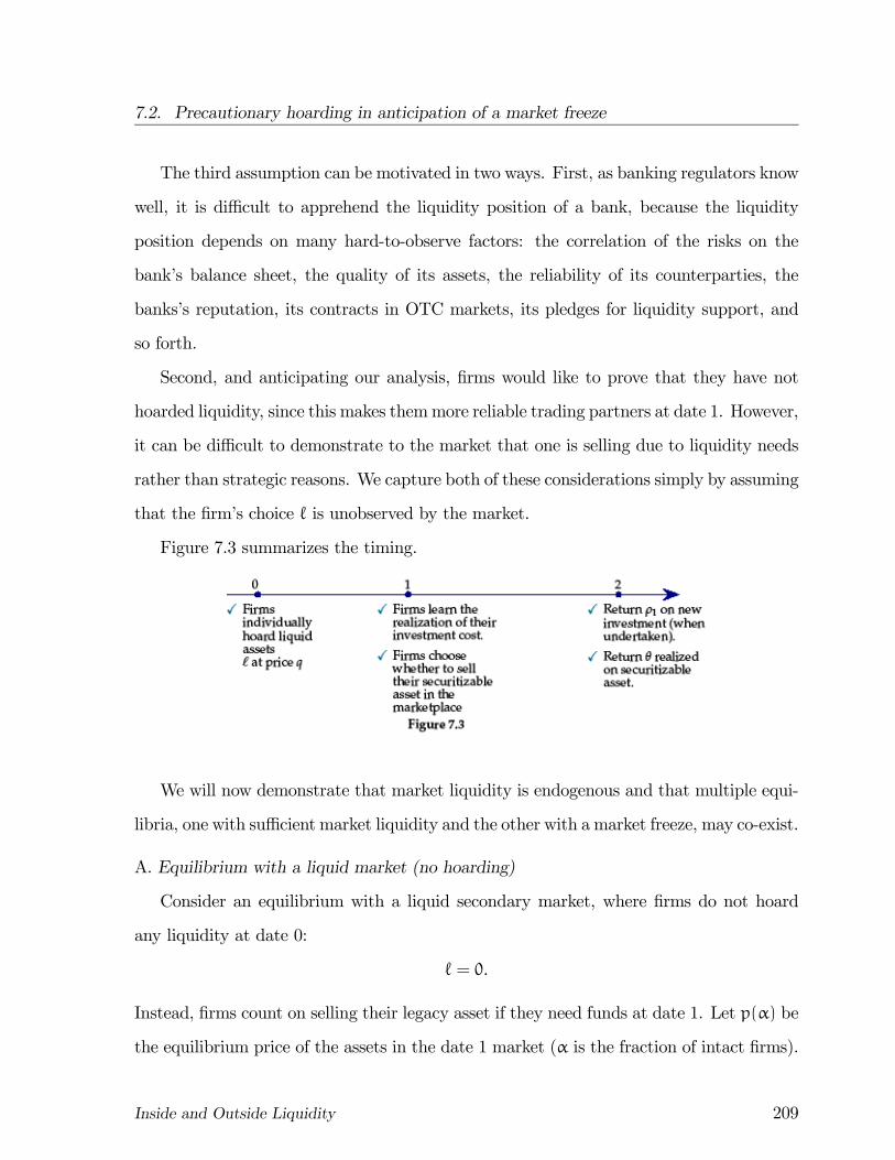
7.2. Precautionary hoarding in anticipation of a market freeze
The third assumption can be motivated in two ways. First, as banking regulators know
well, it is difficult to apprehend the liquidity position of a bank, because the liquidity
position depends on many hard-to-observe factors: the correlation of the risks on the
bank’s balance sheet, the quality of its assets, the reliability of its counterparties, the
banks’s reputation, its contracts in OTC markets, its pledges for liquidity support, and
so forth.
Second, and anticipating our analysis, firms would like to prove that they have not
hoarded liquidity, since this makes themmore reliable trading partners at date 1. However,
it can be difficult to demonstrate to the market that one is selling due to liquidity needs
rather than strategic reasons. We capture both of these considerations simply by assuming
that the firm’s choice ` is unobserved by the market.
Figure 7.3 summarizes the timing.
We will now demonstrate that market liquidity is endogenous and that multiple equi-
libria, one with sufficient market liquidity and the other with a market freeze, may co-exist.
A. Equilibrium with a liquid market (no hoarding)
Consider an equilibrium with a liquid secondary market, where firms do not hoard
any liquidity at date 0:
` = 0.
Instead, firms count on selling their legacy asset if they need funds at date 1. Let p(α) be
the equilibrium price of the assets in the date 1 market (α is the fraction of intact firms).
Inside and Outside Liquidity 209
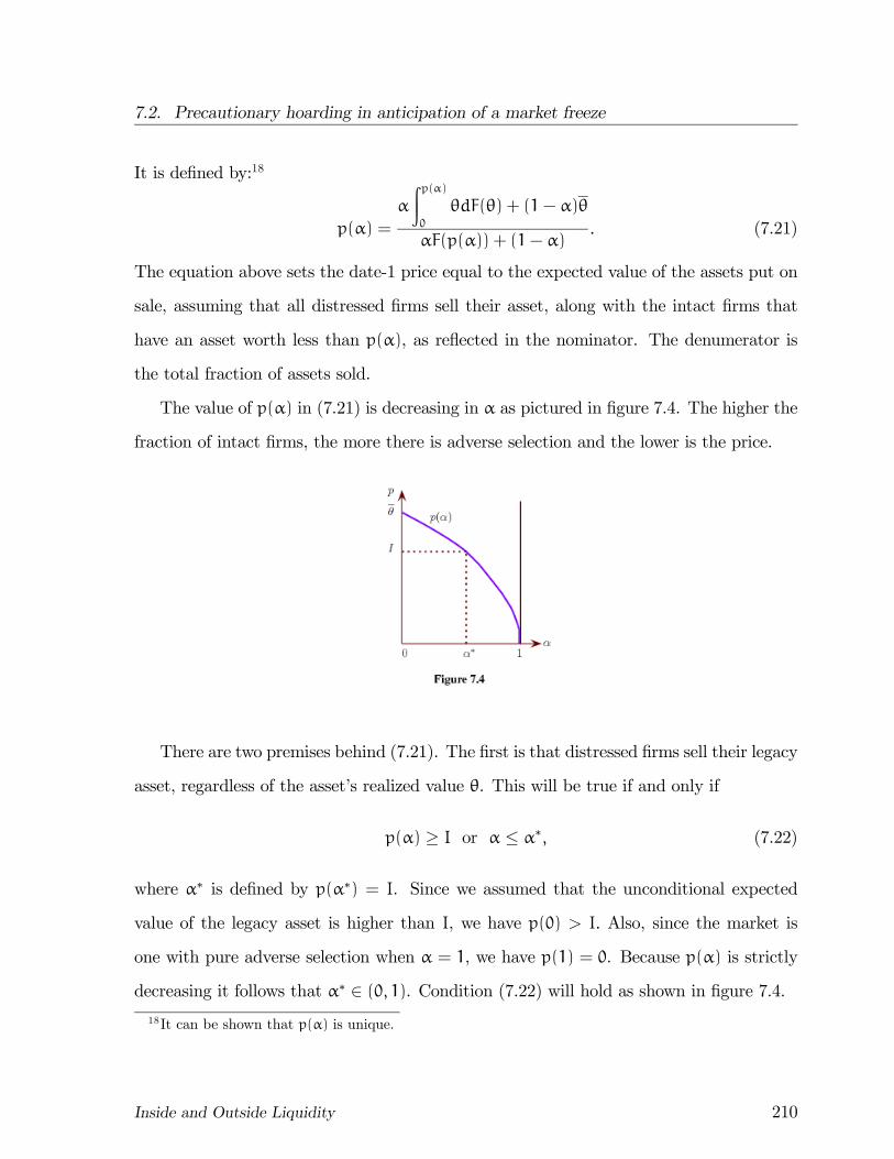
7.2. Precautionary hoarding in anticipation of a market freeze
It is defined by:18
p(α) =
α
Zp(α)0
θdF(θ) + (1− α)θ
αF(p(α)) + (1− α). (7.21)
The equation above sets the date-1 price equal to the expected value of the assets put on
sale, assuming that all distressed firms sell their asset, along with the intact firms that
have an asset worth less than p(α), as reflected in the nominator. The denumerator is
the total fraction of assets sold.
The value of p(α) in (7.21) is decreasing in α as pictured in figure 7.4. The higher the
fraction of intact firms, the more there is adverse selection and the lower is the price.
There are two premises behind (7.21). The first is that distressed firms sell their legacy
asset, regardless of the asset’s realized value θ. This will be true if and only if
p(α) ≥ I or α ≤ α∗, (7.22)
where α∗ is defined by p(α∗) = I. Since we assumed that the unconditional expected
value of the legacy asset is higher than I, we have p(0) > I. Also, since the market is
one with pure adverse selection when α = 1, we have p(1) = 0. Because p(α) is strictly
decreasing it follows that α∗ ∈ (0, 1). Condition (7.22) will hold as shown in figure 7.4.18It can be shown that p(α) is unique.
Inside and Outside Liquidity 210
7.2. Precautionary hoarding in anticipation of a market freeze
The second premise behind (7.21) is that firms do not hoard any liquidity at date 0.
The firm’s net expected utility without liquidity hoarding (` = 0) is:
Uno capital insurance = ρ1 + α
∙p(α) +
Zρ1p(α)
(θ− p(α))dF(θ)
¸+ (1− α)(p(α)− I).
This utility must exceed the utility that the firm obtains by choosing ` = I (because of
our indivisibility assumption, choosing ` ∈ (0, I) is useless, while ` > I would be wasteful),which is
Ucapital insurance = −qI+ ρ1 + α
∙I+ p(α) +
Zρ1p(α)
(θ− p(α))dF(θ)
¸+(1− α)
∙p(α) +
Zρ1p(α)
(θ− p(α))dF(θ)
¸.
Thus the second condition for a liquid market equilibrium is:
(q− 1)I ≥ (1− α)
Zρ1p(α)
[θ− p(α)]dF(θ). (7.23)
This condition is intuitive. It says that the cost of capital insurance, (q−1)I, must exceed
the savings, θ− p(α), associated with not selling an undervalued asset (θ > p(α)) when
distressed. Note in particular that a liquidity premium q− 1 > 0 is required to sustain
an equilibrium without ex ante hoarding of liquidity.
B. Equilibrium with a market freeze (hoarding of liquidity)
In an equilibrium with a market freeze, no transactions take place at date 1. The only
way for a firm to finance an investment is to self-insure by buying short-term assets at
date 0 in the amount ` = I. The condition for an equilibrium with a market freeze is
therefore:
Ucapital insurance = −qI+ ρ1 + αI+ θ
≥ Uno capital insurance = αρ1 + θ,
or
(1− α)(ρ1 − I) ≥ (q− 1)I. (7.24)
Inside and Outside Liquidity 211
7.2. Precautionary hoarding in anticipation of a market freeze
This condition simply says that the net cost of ex ante insurance, (q−1)I, must be smaller
than the value of the foregone investment opportunity, else firms would not want to hoard
liquidity.
Because firms already have all the liquidity they need, there are no gains from trade
at date-1. The date-1 market is a pure lemons’ market, clearing at a zero price with no
trade:
p(α) = E[θ|θ ≤ p(α)] =⇒ p(α) = 0.
Multiple equilibria arise whenever α ≤ α∗ and conditions (7.23) and (7.24) both hold.
Combining these two conditions we get
ρ1 − I ≥Zρ1p(α)
[θ− p(α)]dF(θ), (7.25)
where p(α) is defined by (3.21). Inequality (7.25) is a necessary condition for having both
an equilibrium without any hoarding of liquidity (` = 0, p(α) ≥ I) and an equilibriumwith a market freeze (p(α) = 0, ` = I).
There may also exist intermediate equilibria between these two extremes. In such
equilibria 0 < p < I and 0 < ` < I, such that p+ ` = I. The price is no longer determined
by (7.21), since some of the distressed firms will not sell their legacy asset. In particular,
only distressed firms with θ ≤ ρ1 − ` = ρ1 + p − I < ρ1 will sell; the rest prefer to
keep their legacy asset. As a result, the fraction of assets sold for strategic reaons will
be higher, leading to more adverse selection and a price p < I. Again, the more firms
procure liquidity in advance, the more severe the adverse selection will be and the lower
the price. The equilibrium, as long as it exists, is unique for a given α, since the price
decline per unit of increase in ` is less than one.
Because hoarding liquidity is costly, the Pareto-best equilibrium, given a fixed α, is
the one with a liquid market and no hoarding. The worst equilibrium is the one where
the market freezes and firms have to arrange all of the liquidity in advance. In between
these two is the mixed equilibrium. These comparisons are, of course, relevant only when
Inside and Outside Liquidity 212

7.2. Precautionary hoarding in anticipation of a market freeze
they exist for a given α.
Discussion (public policy). Government supplied liquidity can help or harm depending
on circumstances. To see this, suppose α > α∗ so that the market for legacy assets alone
cannot support the firm’s investment (because p(α) < I; see figure 7.4). Firms would then
like to hoard liquidity in advance so that they can invest at date 1 as discussed above.
If there are no private stores of value, the government can improve matters by supplying
liquidity for this purpose. More generally, if there is a fixed but insufficient supply of
private stores of value, the ex ante insurance market will push the liquidity premium up
to the point where firms become indifferent between hoarding and not hoarding liquidity. If
the liquidity premium in this equilibrium is higher than the government’s cost of supplying
stores of value, the government can improve welfare.
By contrast, when α ≤ α∗, it is socially optimal not to issue government securities (or
more generally to lower the yield on such securities so that (7.23) is violated), because the
equilibrium without hoarding is more efficient than any other equilibrium. Issuing more
liquidity may make no difference to the equilibrium, but would be wasteful (since there is
a dead-weight loss from taxation). If anything, the government may want to reduce the
supply of liquidity, raising its price, which could make the no-hoarding equilibrium more
likely.
The general point here is that an increased supply of liquidity will lower the cost of
liquidity and encourage hoarding. This makes adverse selection in the asset market worse,
inhibiting the functioning of the date-1 market. In this light, the policy of central banks
to accomodate the flight to quality during the subprime crisis (they welcomed deposits
at the central bank) may have had the unintended consequence of delaying the recovery
of asset markets. This conclusion is similar to our earlier point about the advisability of
paying interest on reserves (see subsection 7.1.3) Our analysis underlines the exceptional
informational requirements for a good public policy. Providing cheap public liquidity
Inside and Outside Liquidity 213
7.2. Precautionary hoarding in anticipation of a market freeze
is desirable if markets do not provide enough credit, but it can also crowd out private
markets for liquidity.
Discussion (market versus funding liquidity). Instead of relying on market liquidity by
selling assets, as we have assumed so far, firms could rely on funding liquidity by issuing
securities. We could have developed our analysis in this alternative context. At date 1,
suppose that firms have no assets and hold private information about the value ρ0 of their
date-2 pledgeable income, which is now drawn from a distribution G(ρ0). Suppose further
that the entrepreneurs keep all claims on pledgeable income until date 1 with the intent
to raise funds by selling the claims at date 1 (this could be a cheaper way of saving).
Then those who sell claims because of liquidity needs will on average offer higher quality
claims than those who sell to unload impaired claims. A formula akin to (7.21) obtains:
If the market for funding liquidity does not break down, shares will trade at price p(α)
such that (with double use of notation)
p(α) =αRp(α)0
ρ0dG(ρ0) + (1− α)ρ0αG(ρ0) + (1− α)
.
By contrast, if firms were to invest in stores of value, the market for funding liquidity
would dry up (under conditions similar to those discussed earlier).
Discussion (stigma). One of the potentially counter-intuitive features of the analysis pre-
sented above is that a firm benefits from appearing fragile. Having stored little liquidity
and being forced to go to the asset market for more, rather than being selective about
selling, is reassuring to potential buyers. Yet, common wisdom as well as empirical evi-
dence has it that issuing securities or being forced to sell assets entail a stigma. Financial
institutions even avoid turning to a government agency for help, despite the fact that the
agency may ignore any stigma when it decides to lend. For instance, banks are often
reluctant to borrow at the discount window and countries are often reluctant to apply for
contingent credit lines (CCF) from the IMF. How can we reconcile the theory with this
evidence?
Inside and Outside Liquidity 214
7.2. Precautionary hoarding in anticipation of a market freeze
A potential story has the following two ingredients. First, the bank or the country
typically needs to borrow from other lenders than the central bank or the IMF, respec-
tively, so borrowing from the discount window or a CCL may send a signal of fragility
to these lenders. Second, we need to explain why borrowing from a public body conveys
bad news about an institution. One possible reason is that the need for cash is due to
the unvillingness of better informed lenders and counterparties to continue funding the
institution. Whatever is the reason, our analysis is clearly picking up only a limited aspect
of the story.
Discussion (securitization at date 0).
We have assumed that securities are issued at date 1.19 Would the outcome be different
if the firm could issue securities at date 0, knowing the value of its legacy assets (the
realization of θ), but not yet knowing the cost of the new investment opportunity? To
address this issue, let p0 and p1 denote the date-0 and date-1 equilibrium prices of the
legacy asset. Because legacy assets represent a claim that can be resold at date 1, the
date-0 price p0 is equal, if there is a demand for liquidity at price q, to q times the
expected dividend conditional on the legacy asset being sold at date 0. We consider
possible equilibria in this new situation.
A. No hoarding at date 0
An equilibrium without hoarding at date 0 is observationally equivalent to the no-
hoarding equilibrium when only date-1 securitization is feasible. As before, p1 = p(α) ≥ I.(assuming that α ≤ α∗, of course). Firms wait until date 1 to sell their legacy asset and
do so if they are distressed or if they are intact and face a liquidity shock and θ ≤ p1.19One possible justification is that the firm is in the process of creating an asset that is not yet ready
to be traded at date 0 (e.g. because of severe asymmetric information). This raises interesting avenues
for extending the model. As has been demonstrated empirically, the prospect of issuing securities creates
moral hazard (see Keys, et.al., 2009). So we would expect the distribution F(θ) to be less favorablein the securitization equilibrium than in the market freeze equilibrium. (For more on this, see Aghion,
et al, 2004, who take a mechanism design approach to securitization under moral hazard. See also
Faure-Grimaud and Gromb, 2004, as well as Parlour and Plantin, 2008.)
Inside and Outside Liquidity 215
7.2. Precautionary hoarding in anticipation of a market freeze
There is no trade of the legacy asset as long as p0− (q−1)I ≤ p1, that is, as long as thereare no gains to trading early even if firms knew that they will sell at date 1, regardless
of the liquidity shock. In particular, there is an equilibrium with p0 = 0 and no trade,
supported by the off-equilibrium belief that any attempt to sell at date 0 has a purely
strategic motive.
Thus, the no-hoarding equilibrium in the earlier model is robust to the possibility of
date 0 trading of the legacy asset under adverse selection.
B. Hoarding at date 0
In a hoarding equilibrium, p0 = p1 = 0 without any trading of assets. Firms will
hoard their own liquidity (which requires (7.24) to be satisfied). Like the no-hoarding
equilibrium, the hoarding equilibrium is robust to early trading.
C. Other equilibria
Could there be other equilibria? Intuitively, there are two forces that determine the
equilibrium price. First, we would expect “more adverse selection” at date 0, since at date
1 there are at least some potential sellers who experience a liquidity shock. Ceteris paribus
the sellers with low-quality assets are more eager to sell at date 0 (i.e. unconditionally)
than those who have better quality assets and are more willing to wait to see whether
they will end up distressed or intact at date 1. Second, selling claims at date 0 creates
stores of value for the buyers and this has social value since q > 1. This could favor
date-0 trading, though the benefit of saving by not selling also needs to be taken into
consideration.
Let us look for an equilibrium in which some trade occurs at date 0. We are led to
consider two cases:
Case 1: p1 < I. In this case there are no gains from trade at date 1 so the only market
for assets is at date 0. A firm that wants to invest at date 1 will have to buy liquidity at
date 0, regardless of whether it sells the asset at date 0 or holds it to maturity. Type θ
Inside and Outside Liquidity 216
7.2. Precautionary hoarding in anticipation of a market freeze
decides to sell at date 0 rather than hold the asset to maturity if and only if
p0 − (q− 1)I+ [ρ1 − (1− α)I] ≥ θ− (q− 1)I+ [ρ1 − (1− α)I] (7.26)
or
p0 ≥ θ.
The term on the left hand side of (7.26) includes the proceeds from selling at date 0, the
cost of buying I units of liquidity to weather a low shock at date 1, and the net benefit
of investing at date 1. The right-hand side has a corresponding interpretation, reflecting
the value of investing and holding the asset to maturity. Let θ∗ be the cutoff for selling
the asset. Note that p0 = qm−(θ∗), where m−(θ∗) = E(θ|θ ≤ θ∗) is the expected the
value of the assets put up for sale. The equilibrium cutoff, if it is interior, satisfies:
qm−(θ∗) = θ∗.
For instance, in the case of a uniform distribution, m−(θ∗)/θ∗ = 1/2, so trade occurs at
date 0 (and involves all types) if and only if q ≥ 2.
Case 2: p1 ≥ I. In this case, there is a need to buy liquidity at date 0 only if the assetis sold at date 0. If it is sold at date 1, the price at date 1 is sufficient to cover the
investment need.
Selling at date 0 yields as before
p0 − (q− 1)I+ [ρ1 − (1− α)I].
On the other hand, the value of holding off on selling until date 1 is
[ρ1 − (1− α)I] + p1 if θ ≤ p1
and
[ρ1 − (1− α)I] + αθ+ (1− α)p1 if θ ≥ p1.
Inside and Outside Liquidity 217
7.2. Precautionary hoarding in anticipation of a market freeze
Again, only types below some cutoff θ∗ sell at date 0. Futhermore, a necessary condition
for trade at date 0 is
p0 − (q− 1)I ≥ p1.
Since only types above θ∗ can sell at date 1, we must have p1 ≥ θ∗ and therefore an
equilibrium of the assumed kind exists only if there is a θ∗ such that:
qm−(θ∗)− (q− 1)I = p1(θ∗)
where p1(θ∗) is the solution to
p1 =
α
Zp1θ∗θdF(θ) + (1− α)
Zρ1θ∗θdF(θ)
α£F(p1)− F(θ
∗)¤+ (1− α)[1− F(θ
∗)].
Discussion (mixing financial muscle and adverse selection). Bolton, Santos and Scheinkman
(2009) argue that adverse selection may increase liquidity hoarding, but for a somewhat
different reason. Their model involves two sets of players: long-term arbitrageurs (sov-
ereign wealth funds, pension funds,...), which hoard costly liquidity to buy assets at cash-
in-the-market prices (that is, at a discount) and firms, which before the date of reckoning,
i.e. before the final return on a project is realized, face a liquidity need. Uncertainty
about the final profit of each firm unfolds gradually, and efficient trade involves trading as
late as possible before the date of reckoning. Delaying trade reduces the quantity hoarded
by long-term investors, as they do not have to acquire intermediate dividends.20 However
late trading may not be feasible as Bolton et al posit that adverse selection increases over
time. The prospect of a market freeze then forces early trading and therefore more liq-
20The paper assumes all-or-nothing trades, that is, a firm’s cash flow cannot be split into securities
with different maturities. Otherwise the long-term investors could economize on costly liquidity hoarding
by purchasing only the securities’ late dividends, and not the early ones.
In the paper, there are four dates: 0, 1, 2, 3. The ST traders have preferences c0 + c1 + c2 + δc3 with
δ < 1. Thus ST traders do not need to trade before date 2, at which date they need to sell only the claim
to the last dividend.
Inside and Outside Liquidity 218
7.3. Summary
uidity hoarding. Increasing adverse selection provides incentives for early trading, which,
if tranching is infeasible, induces an inefficient amount of liquidity hoarding.
7.3 Summary
This chapter has shown that the inability of firms to write state-contingent contracts on
the available supply of liquidity at date 1 may lead to excess investments in liquidity at
date 0 as well as to a wrong allocation of liquidity at date 1. When liquidity is used to buy
distressed assets, investments in liquidity tend to be excessive due to wasteful competition
for ex-post rents. However, our analysis of predatory hoarding of liquidity also shows that
decentralized choices regarding liquidity do not necessarily cause inefficiencies. With our
particular structure, spot markets are often capable of replicating the fully coordinated
solution. And even when spot markets cannot duplicate the coordinated solution, the
government is not always able to increase welfare by regulating liquidity. If the problem
is a reluctance on the part of firms with excess resources to reallocate these resources to
distressed firms, then increasing government supplied liquidity may simply lead to more
assets being employed suboptimally at date 1.
We also showed that precautionary hoarding of liquidity may have the unintended
consequence of a market freeze. Buyers may question the sellers’ motives for selling their
assets if they know that the sellers have a sufficiently large cushion of cash. Liquidity
hoarding encourages market freezes (and conversely). While the laissez-faire outcome may
involve excessive liquidity hoarding, in some circumstances precautionary hoarding is de-
sirable. Distinguishing between two cases with such radically different policy implications
requires detailed information and makes the policy task very challenging.
An extension that would be interesting and relatively straightforward to explore is
to have the fraction of intact firms be random. This would be one way of introducing
an aggregate shock.21 Given that the shock is aggregate, it should be possible to write
21Allen and Gale (1994, 2005) allow for such aggregate shocks in their models.
Inside and Outside Liquidity 219

7.3. Summary
contracts on the state. The characteristics of an optimal supply of liquidity (eg by gov-
ernment) when the idiosyncratic shocks must be handled through spot markets would be
interesting to understand.
While the two motives leading to overhoarding of liquidity (predatory and precaution-
ary hoarding) seem realistic, we certainly do not believe overhoarding is the rule. Indeed,
the subprime crisis appears to have been triggered in part by underhoarding of liquidity
and excess leverage among financial institutions. Many commercial and investment banks
(and insurance companies, like AIG) relied on short-term financing for continued fund-
ing, instead of investing in short-term assets that could have been used when liquidity
got scarce. These institutions, which benefitted from cheap sources of capital thanks to
an implicit guarantee from the governments, took increasingly risky gambles with more
severe maturity mismatches despite warnings. As Farhi and Tirole (2009b) argue, ma-
turity mismatches are subject to strategic complementarities. Central banks are unlikely
to maintain interest rates low in order to keep a single institution alive. By contrast,
when faced with a widespread maturity mismatch, the centrals banks have no choice but
keeping the interest rate very low, at the cost of substantial distortions to the economy;
and so they did.
Inside and Outside Liquidity 220
Chapter 8
Specialized inputs and secondary
markets
This chapter continues to analyze the implications of firms relying exclusively on secondary
markets for their liquidity needs. As in the previous chapter, we assume that firms do
not coordinate their balance sheet choices, but while in section 7.1, the motive is self-
insurance. Firms hoard an input, which we will generically call a “widget.” This input is
needed to keep long-term assets operative, much as in the basic model we studied Parts
II and III of the book. A widget could stand for many things. It could literally be a part
that is needed for continuing production; it could be a service or knowledge that is needed
to make the asset productive; or, as in the application of section 8.2, it could stand for
collateral secured on international financial markets.
In section 8.1, ex ante identical firms invest both in illiquid, long-term assets and in
widgets. Widgets are used at date 1 to help those firms that end up being distressed to
weather the shock. Widgets however need not be in the right hands, and so in the absence
of an ex ante coordinated pooling arrangement, a secondary market will open to allow
transfers of widgets held by intact firms to distressed firms. As in section 7.1, buyers may
not have enough financial resources to acquire the needed widgets at a price that dominates
the alternative use of widgets. Therefore, financial constraints may lead to an inefficient
reallocation of widgets through the secondary market. One of the central question we
221
8.1. Secondary markets for specialized inputs
will address is whether firms will tend to underhoard those widgets. Intuitively, one might
reason that a low resale price should discourage investments in widgets: A firm that ends
up on the sell side would have to sell widgets at a discount relative to the social value.
A firm that ends up on the buy side would get widgets at a discount. Both forces would
seem to favor less hoarding and more reliance on the date-1 market. We will show however
that this intuition is wrong in our model. In our equilibrium there is no underhoarding,
even though the date-1 widgets sell at a discount.1
Section 8.2 applies the model in section 8.1 to an international context. Widgets refer
to dollars, i.e., international liquidity. Our analysis of international liquidity in Chapter
6 presumed that the firms optimally coordinate their liquidity plans and focused on the
value of international financial markets as a source of insurance. In section 8.2, the focus is
on international liquidity (dollars) as an input in the production process. For this reason
we assume that there are no macroeconomic shocks. Like the widgets in section 8.1,
dollars are needed for re-investment. We are interested in possible inefficiencies arising
from the firms’ uncoordinated purchase of dollars at date 0 — in particular the possibility
that firms will not secure enough dollars at date 0 (or equivalently, that they will borrow
excessively on the international markets).
8.1 Secondary markets for specialized inputs
8.1.1 Model and two benchmarks
We assume that firms are ex ante homogenous but ex post heterogenous. Our model is
again one where distressed assets are salvaged by intact firms. But we turn the model
of section 7.1 on its head by assuming that distressed firms do not sell their assets to
intacts, but rather that intact firms sell their assets to distressed firms. Those in distress
buy rather than sell. Secondary markets will trade liquid (ST) assets rather than illiquid
1Caballero and Krishnamurthy (e.g. 2001, 2002) explain their results using this kind of intuition. We
will discuss why the “cheap widget” intuition fails in our setting.
Inside and Outside Liquidity 222
8.1. Secondary markets for specialized inputs
(LT) assets. And liquid assets rather than illiquid ones will sell at a discount relative to
their date-0 prices.
At date 0 a representative entrepreneur has wealth A and invests
• I in LT assets, delivering, at date 2, ρ1I in total income and ρ0I in pledgeable
income, provided that the assets are still in use at date 2;
• ` in ST assets (widgets), where ` is the number of units received at date 1 in returnfor a date-0 investment g(`). For simplicity, we assume that the marginal cost of
producing widgets is constant, that is g(`) = q`, where q ≥ 1. Firms that invest inthe LT asset also have access to the ST widget technology.
At date 1, a firm will be
• intact with probability α, where “intact” means that the firm does not need any
widget. Its long-term investments deliver total value ρ1I and pledgeable income ρ0I
at date 2;
• distressed with probability 1−α, where “distressed” means that it takes one widget
per unit of long-term investment to deliver the date-2 returns of intact firms. A
distressed unit that does not get a matching widget at date 1 generates no income
at date 2.
As in Chapter 7, there is no aggregate uncertainty. Widgets at date 1 can be converted
to an alternative use (the “baseball field” of the parable in Chapter 7) with per unit value2
ρ < q.
Only an intact firm will face the choice of converting its widgets to the alternative use.
A. Second-best benchmark (full coordination)
2In this model, unlike the one in chapter 7, there will be no inefficiencies without an outside outside
option.
Inside and Outside Liquidity 223
8.1. Secondary markets for specialized inputs
As a benchmark, we first consider policies in which firms coordinate their date-0
investments and the date-1 use of widgets. Because there is no aggregate uncertainty
and the investment and use of widgets are fully coordinated, there is never any excess
accumulation of widgets. No widgets are converted to the alternative use (since ρ < q)
and so we can, without loss of generality, assume that widgets are only used by the
distressed firms.
How much will the firms invest in widgets (ST assets)? Intuitively, it is worth investing
in widgets whenever they are cheap enough (q is small) or the probability of distress (1−α)
is high. To demonstrate this formally, consider the following social planning program.
maxI,`,m
(ρ1 − ρ0) [αI+ (1− α)(`+m)] (8.1)
s.t.
α` ≥ (1− α)m, (i)
I+ q`−A ≤ αρ0I+ (1− α)ρ0(`+m), (ii)
`+m ≤ I. (iii)
The choice variables are: the date-0 investments I in LT assets and ` in ST assets
(widgets) and the date-1 transfer m of widgets from intact firms to distressed firms. The
objective is to maximize the representative entrepreneur’s gross utility, which is equal
to the social surplus, because the budget constraint must bind at an optimum. The
first constraint is the date-1 aggregate resource constraint; it requires that the transfer of
widgets to the distressed firms cannot exceed the supply of widgets by the intact firms. As
noted above, this constraint could be written as an equality, because it would be wasteful
to hoard more widgets than will be used by the intacts (recall that there is no aggregate
uncertainty). The second constraint is the date-0 resource, or budget constraint. The
third constraint is technological: the continuation scale cannot exceed I.
Let the date-1 continuation scale be i = `+m. Constraint (i), as an equality, implies
Inside and Outside Liquidity 224
8.1. Secondary markets for specialized inputs
m = αi and ` = (1−α)i. Noting that m = αi and ` = (1−α)i, we can then rewrite the
social program as
maxI,i
αI+ (1− α)i (8.2)
s.t.
I+ q(1− α)i−A ≤ αρ0I+ (1− α)ρ0i, (i)
i ≤ I. (ii)
In this program, the firm chooses the initial scale I and the continuation scale i with
the continuation i assured by choosing m and ` according to m = αi and ` = (1 − α)i.
The budget constraint, as an equality, allows us to subtitute out I and write the social
objective (dropping constants) as
maxi[α(ρ0 − q) + (1− αρ0)]i
It follows that it is socially optimal to continue at full scale (choose i = I) whenever
αq < 1. (8.3)
As a weak inequality, the condition is necessary for buying widgets at date 0 (` > 0).
As one would expect, liquidity hoarding is more desirable, the higher the probability of
distress and the cheaper the acquisition of liquidity.
B. Another useful benchmark: the autarky case.
Even though we will allow a spot market for reallocating widgets shortly, it is also
useful to study the autarky case as a benchmark. Indeed, for very low levels of ρ0,
distressed firms have little with which to pay for widgets and so, even in the presence of
a secondary market, trade will be minimal and the outcome will resemble autarky.
In autarky, each firm provides for its own widgets: there is no coordination or reallo-
cation of widgets. Given the linear technology, a firm has two relevant choices. It can bet
Inside and Outside Liquidity 225
8.1. Secondary markets for specialized inputs
all its money on being intact and use its capital to maximize the initial scale without any
investment in widgets. Alternatively, it can allocate its capital equally between the initial
investment I and widgets ` = I so that it can continue at full scale even when it ends
up in distress. The latter strategy will waste part of the initial investment in widgets,
because if the firm ends up being intact, it recovers only ρ < q per unit. On the other
hand, the former strategy will waste the initial investment if the firm ends up in distress.
With the first strategy the maximal scale and the entrepreneur’s gross payoff are:
II =A
1− αρ0, (8.4)
(8.5)
UgI =
(ρ1 − ρ0)A1α− ρ0
. (8.6)
The maximal scale associated with investing in widgets (the second strategy) is given
by
I+ qI ≤ A+ ρ0I+ αρI,
yielding
I =A
1+ q− (ρ0 + αρ). (8.7)
So the gross payoff to the entrepreneur is
UgII =
(ρ1 − ρ0)A
1+ q− ρ0 − αρ. (8.8)
Comparing UgI and U
gII we find that hoarding is optimal in autarky if and only if
α(1+ q)− α2ρ < 1. (8.9)
There is an important difference between the coordinated hoarding criterion (8.3) and
the autarky hoarding criterion (8.9). In autarky, the firm is forced to hoard the initial
investment (` = I) in order to continue at full scale, while in the coordinated solution
it suffices to hoard ` = (1 − α) I, because liquidity is optimally shared. So, hoarding
Inside and Outside Liquidity 226
8.1. Secondary markets for specialized inputs
is more costly in autarky and the cut-off criterion for hoarding therefore more stringent.
If there is hoarding in autarky, there will be hoarding in the coordinated case as well.
Moreover, there is a region of α for which there is no hoarding in autarky even though
there is hoarding in the coordinated case.3
8.1.2 Self-provision of liquidity with resale
Suppose now that at date 1 a spot market opens in which the intact firms may sell their
widgets (for which they have no use) to distressed firms. The distressed firms pay for
these widgets by issuing claims on their pledgeable income. In addition, the distressed
firms can rescue long-term assets by using widgets procured at date 0. We first investigate
the case where widgets have no alternative use and hence are all sold to distressed firms.
• No alternative use for widgets (ρ = 0)
In this section, we show that without an outside option for liquidity (a “baseball
field” in the parable of the introduction to Section 7.1), trading in a date-1 spot market
always achieves the second-best outcome. We do it by showing that the firm’s optimization
program is equivalent to the the second-best, full-coordination program described in sub-
section A above.
Let p be the date-1 spot price for widgets. The firm’s problem is solved by the program
maxI,`,m
(ρ1 − ρ0) [αI+ (1− α)(`+m)] (8.10)
s.t.
pm ≤ ρ0(`+m), (i)
I+ q`−A ≤ α(ρ0I+ p`) + (1− α)[ρ0(`+m)− pm], (ii)
`+m ≤ I. (iii)
3Let eα(ρ) denote the solution of:α(1+ q)− α2ρ = 1.
Note that eα(q) = 1q(the cutoff found in the perfectly corrdinated solution), that eα(0) = 1
1+q, and that
for all ρ < q, eα(ρ) < 1q.The region with hoarding only in the coordinated case is the interval
¡eα(ρ¢ , 1q).
Inside and Outside Liquidity 227
8.1. Secondary markets for specialized inputs
Constraint (i) is the firm’s date-1 liquidity constraint, which limits purchases m to
no more than the pledgeable income. Constraint (ii) is the date-0 budget constraint and
constraint (iii) limits the continuation to the initial scale of investment. The objective
function maximizes the entrepreneur’s gross utility; because the budget constraint will
bind, the entrepreneur obtains all the social surplus.
Since an intact firm has no other outlet for its stored widgets than the spot market,
all the widgets must in the date-1 equilibrium be transferred from the intact firms to the
distressed firms (without aggregate certainty, there is no point in buying more widgets
than are needed in equilibrium). This gives the equilibrium condition
α` = (1− α)m. (8.11)
Adding up the individual firms’ liquidity constraints (i) and the aggregate date-1 liquidity
constraint (8.11), yields the following condition which p must satisfy:
p ≤ ρ0α. (8.12)
To build some intuition for the solution, it is helpful to consider the relative attractive-
ness of investments in short-term and long-term assets, ignoring the liquidity constraint
(i) and the feasibility constraint (iii). That is, we look at the benefit of `,m and I relative
to the budget expenditure.
Consider first the choice of acquiring widgets in the primary versus the secondary
market: A firm can procure widgets ` at date 0 for price q or widgets m at date 1
for price p. Suppose p > q and m > 0 and consider the effect of substituting a unit
of ` for a unit of m in the firm’s program (8.10). This will loosen the firm’s budget
constraint (ii) by (p−q) > 0, loosen the firm’s liquidity constraint (i) by p and leave the
firm’s objective and the technological constraint (iii) unaltered. The entrepreneur could
therefore do strictly better by reducing m all the way down to zero. But at zero demand,
the date-1 equilibrium price cannot be positive, a contradition. So in equilibrium, we
Inside and Outside Liquidity 228

8.1. Secondary markets for specialized inputs
must have p ≤ q. Running the substitution argument in reverse, we see that p < q
implies that the liquidity constraint (8.10)(iii) must bind, else the entrepreneur could do
better by substituting m for `. Note also that the liquidity constraint (8.10)(i) can bind
only if p ≥ ρ0. We have established that the equilibrium price must satisfy:
ρ0 ≤ p ≤ q. (8.13)
With these preliminaries we proceed to analyze the four regions of α that characterize
the solution to program (8.10), and show that in the absence of an alternative use for
liquidity at date 1, the outcome will be efficient.
Region I (0 < α ≤ ρ0/q): Widgets are resold at their purchase price
In this region, there are few intact firms (α is small), and so widgets are in high demand
and command a high price in the secondary market. For this reason, we conjecture that
the equilibrium price will be at its upper bound, p = q, (see (8.13)). We also conjecture
that the firm’s liquidity constraint is slack at this price and relax the firm’s program by
ignoring this constraint. We will come back to verify that both conjectures are true in
equilibrium in the indicated range of α.
When p = q the firm’s budget constraint (8.10) (ii) can be written
I+ q(1− α)(`+m)−A ≤ αρ0I+ (1− α)ρ0(`+m). (8.14)
In the relaxed program, where the firm’s liquidity constraint is dropped, only the choices
I and i = `+m matter. We can therefore impose the additional constraint
m = αi and ` = (1− α)i (8.15)
and restrict the firm to chosing ` and m along this ray. Substituting (8.15) and p = q
into the firm’s liquidity constraint we get
αq ≤ ρ0 < 1 (8.16)
Inside and Outside Liquidity 229
8.1. Secondary markets for specialized inputs
We see that on the ray (8.15) the validity of the liquidity constraint does not depend on
i. The constraint will be satisfied if and only if α ≤ ρ0/q, which is the upper bound of
Region I. So, the solution to the relaxed program (without liquidity constraint) satisfies
the liquidity constraint in Region I when p = q. Finally, it is immediate that the market
equilibrium condition (8.11) holds whenever the firm chooses ` andm along the ray (8.15);
indeed, the ray condition is equivalent to the market equilibrium condition as we noted
earlier.
We have verified that the equilibrium in Region I entails p = q with the representative
firm choosing m = αI, ` = (1− α)I, where (using the budget constraint)
I =A
1+ q(1− α)− ρ0. (8.17)
In Region I, the firm’s liquidity constraint will be slack until α hits its upper bound.
Conversely, note that if the liquidity constraint is slack, we must have p = q or else the
firm would do better either by buying all its liquidity at date 0 or at date 1, violating the
equilibrium condition. The ex post competition for scarce liquidity goes hand in hand
with a non-binding liquidity constraint.
It is more surprising that the uncoordinated equilibrium in Region I is actually the
same as the second-best solution obtained by coordinating liquidity purchases (as in the
benchmark model discussed earlier). This can be verified directly by solving the second-
best program (8.1). But it is more instructive to check that the firm’s program (8.10)
is identical with the second-best program when p = q. Note first that the liquidity
constraint in the firm’s program is irrelevant in Region I. Condition (8.15) assures that
the date-1 resource constraint in the second-best program is satisfied regardless of i.
When one substitutes p = q and (8.15) into the firm’s budget contraint (8.14) and the
second-best program (8.1), the two programs can be seen to be identical. Finally, note
that αq < 1, so the second-best program has i = I.
Region II (ρ0/q < α < ρ0/ρ): Resale at a discount
Inside and Outside Liquidity 230
8.1. Secondary markets for specialized inputs
When α > ρ0/q, the solution in Region I no longer works, because it violates the
firm’s liquidity constraint. In Region II, therefore, we expect the liquidity constraint to
bind. We proceed with this conjecture and verify that it is indeed true in equilibrium.
The binding liquidity constraint pm = ρ0(` +m), together with the market clearing
condition α` = (1− α)m, implies that the market price must be
p =ρ0α< q. (8.18)
The inequality follows from the lower bound of Region II. If we insert this equilibrium
price into the firm’s liquidity constraint we getm = αi, implying that ` = (1−α)i. So, the
liquidity constraint at the equilibrium price coincides with the date-1 resource constraint
of the second-best program. Furthermore, the firm’s budget constraint becomes
I+ q(1−α)i−A ≤ αρ0i+ (1−α)ρ0i+ [αp`− (1−α)pm] = αρ0i+ (1−α)ρ0i. (8.19)
Therefore, the budget constraint in the firm’s program is identical to the budget constraint
in the second-best program. We conclude that the second-best and first-best programs
coincide again and hence the solution in Region II will be efficient. The investment I will
be given by (8.17) and i = I. In particular, firms will buy a strictly positive amount of
widgets at date 0.
The reader may find it surprising that efficiency obtains in Region II despite an under-
valued resale price (p < q). After all, intact firms sell their widgets at too low a price and
distressed firms buy them up at an equally low price. Either way, ex ante firms should
have an incentive to underhoard widgets. However, this reasoning misses the point that
widgets relax the liquidity constraint of distressed firms: The more widgets distressed
firms own, the higher their funding liquidity, and so the more widgets they can purchase:
see the firms’ liquidity constraint (8.10)(i). And the lower the secondary market price p,
the more distressed firms can lever up the pledgeable income that stems from their own
widgets. As a result, under constant returns to scale there is neither underhoarding nor
Inside and Outside Liquidity 231
8.1. Secondary markets for specialized inputs
overhoarding.4
• Widgets have an alternative use (ρ > ρ0q)
Without the outside option, Region II would extend all the way to α = 1/q and after
that i = I. The uncoordinated solution would coincide with the coordinated solution for
all α. To introduce a source of inefficiency, we assume that there is an alternative use for
widgets (a "baseball field" in the langue of Chapter 7), which intact firms can make use
of. The value of this use is assumed to be ρ > ρ0q, so that ρ0/ρ < 1/q, which is the
point at which it becomes inefficient in the second-best to continue.
In Region II, as α increases, the equilibrium price p = ρ0/α falls. The alternative use
of widgets implies
p ≥ ρ (8.20)
This constraint binds whenever
α >ρ0ρ, (8.21)
which defines the upper bound of Region II.
Region III (ρ0/ρ < α < α0 < 1/q).5 Widgets are in part converted to the alternative
use.
Other things equal, ρ0 has to be sufficiently small to satisfy (8.21) A small ρ0 means
that the purchasing power of the distressed firms is small; the smaller it is, the more of
4This discussion raises the issue of what would happen if relatively cheap stores of value (Treasury
bonds) were available as well. Would they crowd out the hoarding of widgets, offering a better yield
while allowing firms to obtain refinancing? We have not conducted a full analysis, but we conjecture that
the answer is “no”. If widgets are expected to be cheap in the secondary market, then firms will hoard
substantial amounts of Treasury bonds to take advantage of fire-sale prices. This will raise the price of
widgets until the firms are indifferent between hoarding widgets and hoarding Treasury bonds.
When Treasury bonds are costless (their price is equal to 1), the liquidity constraint is never binding
as firms have access to costless liquidity. Then regardless of the value of other parameters, the widgets
trade at no discount in the secondary market: p = q.
5The upper limit α0 will be defined when we discuss Region IV.
Inside and Outside Liquidity 232

8.1. Secondary markets for specialized inputs
the intact firms’ widgets will go to the alternative use. To be more precise, the liquidity
constraint will allow a firm to purchase widgets (at price p = ρ) up to the amount
m =ρ0`
ρ− ρ0. (8.22)
Consider an equilibrium in which some liquidity is converted to the alternative use
and so the market price for liquidity is
p = ρ.
There are two cases to consider:
• The firm withstands the shock:
It then purchases the maximal amount (8.22) and so, as `+m = I
` =ρ− ρ0
ρI
This yields gross utility:
UgII =
(ρ1 − ρ0)A
1+ qρ−ρ0ρ
− αρ.
• The firm does not withstand the shock:
This strategy, as usual, yields gross utility:
UgI =
(ρ1 − ρ0)A1α− ρ0
.
For firms to be willing to accumulate liquidity, one must have
UgII ≥ UgI
or
1+ qρ− ρ0
ρ− αρ ≤ 1
α− ρ0. (8.23)
Let α0 be the highest α satisfying (8.23), implicitly defined by
1+ qρ− ρ0
ρ− α0ρ =
1
α0− ρ0.
Inside and Outside Liquidity 233
8.1. Secondary markets for specialized inputs
Finally, we check that there is enough liquidity on the market to support the suggested
solution. This requires
α` ≥ (1− α)m,
which indeed holds, by (8.22), whenever
α ≥ ρ0ρ, (8.24)
that is, in Region III.
If (8.24) is slack, then there is excess liquidity in the market and some of the wid-
gets will be converted to the alternative use. The wasted amount is found (after some
manipulations) to be
w = α`− (1− α)m =αρ− ρ0
ρI
=
µαρ− ρ0
ρ
¶⎛⎜⎜⎜⎝ A
1+ q
µρ− ρ0
ρ
¶− αρ
⎞⎟⎟⎟⎠ .Simple computations show that
∂w
∂ρ0< 0.
A smaller pledgeable income implies more waste of liquidity.
Region IV (α > α0). No investment in liquidity
Firms may not find it attractive to hoard liquidity at all when the spot price is ρ. This
arises when (8.23) is violated. Firms will not invest in liquidity when α > α0. Note that
α0 <1
q.
Thus the region over which there is investment in liquidity is smaller than that in the
coordinated case, giving rise to an inefficiency.
Inside and Outside Liquidity 234
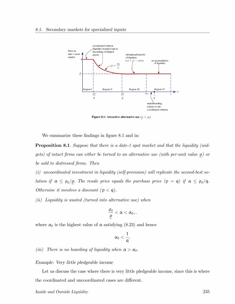
8.1. Secondary markets for specialized inputs
We summarize these findings in figure 8.1 and in:
Proposition 8.1. Suppose that there is a date-1 spot market and that the liquidity (wid-
gets) of intact firms can either be turned to an alternative use (with per-unit value ρ) or
be sold to distressed firms. Then
(i) uncoordinated investment in liquidity (self-provision) will replicate the second-best so-
lution if α ≤ ρ0/ρ. The resale price equals the purchase price (p = q) if α ≤ ρ0/q.
Otherwise it involves a discount (p < q).
(ii) Liquidity is wasted (turned into alternative use) when
ρ0ρ< α < α0, .
where α0 is the highest value of α satisfying (8.23) and hence
α0 <1
q.
(iii) There is no hoarding of liquidity when α > α0.
Example: Very little pledgeable income
Let us discuss the case where there is very little pledgeable income, since this is where
the coordinated and uncoordinated cases are different.
Inside and Outside Liquidity 235
8.1. Secondary markets for specialized inputs
A firm that wants to continue in the distressed state can count on getting m widgets
from the spot market and therefore will buy at most ` = I−m widgets at date 0. When
ρ0 is very small, m will be very small and ` will be close to I. If ρ is also small, the
proceeds from selling widgets at date 1 will be small. In the non-coordinated case, then,
for
ρ0 ' 0,
the decision whether to hoard liquidity or not at date 0 is very close to the autarky
decision, where the firm had to choose between ` = I and ` = 0. In that case, we found
that the firm would not buy any widgets if α ≥ 11+q.6 This is a lower cut-off than the
second-best α ≥ 1q. So, if ρ0 ' 0, and ρ ' 0, we will have a range of α such that firms
in the spot market choose not to buy any widgets, while firms in a coordinated market
would buy ` = (1−α)I. In this limited range (1/(1+ q), 1/α) , there is “under-hoarding”
of widgets relative to the second-best. On the other hand, when α < 11+q, we know that
the firm will procure ` = I widgets in the autarky solution and hence ` = I−m ≈ I, whenρ0 ' 0. In this case, there is “over-hoarding” of widgets relative to the second best.
8.1.3 Policy
Regions I and II deliver the coordinated solution so no policy intervention is called for.
Similarly, the optimal solution (` = 0) prevails when α ≥ 1/q, which is a subset of RegionIV.
Liquidity is wasted in Region III. However, encouraging firms to hoard more liquidity
can only reduce welfare, since the problem is that the secondary market price is too
low (p = ρ). Any extra liquidity will only be wasted as it goes to the alternative use.
Indeed, “under-hoarding” and “over-hoarding”, as discussed above, refer to equilibrium
investments in liquidity relative to the second-best, coordinated benchmark studied in
part A. Therefore, liquidity regulation, assuming it is feasible, does not improve welfare.
6Note that for ρ0 = 0, (8.23) is equivalent to α ≤ 1/(1+ q) as ρ tends to 0.
Inside and Outside Liquidity 236
8.1. Secondary markets for specialized inputs
Consider the “over-hoarding” case and assume that the government can force firms to
hoard less than I, say, the second-best level (1− α)I. For ρ0 small, the distressed firms
will not be able to buy liquidity to make up the shortage (for example acquire αI, when the
liquidity is constrained to the coordinated level). Similarly, forcing firms to hoard more
in the "under-hoarding" case will not help as the extra liquidity will not get transferred
at date 1. The firms de facto live in autarky as they cannot count on acquiring liquidity
when distressed.
8.1.4 Asymmetries and the emergence of underhoarding
This section studies a two-sector variant of the previous model. Liquidity is being pro-
duced by one group of firms at date 0, while another group of firms need liquidity at
date 1. Because the latter may have little to offer in exchange for liquidity, the former
may produce (or procure) insufficient amounts of liquidity. Due to the asymmetry, the
production of liquidity will have no direct benefit for the producers and this eliminates the
countervailing effect that rules out underhoarding in the symmetric model of the previous
section.
Consider the two-sector economy described in Figure 8.2. Sector 1 consists of a contin-
uum of identical entrepreneurial firms of the type studied in Section 3.2. A representative
entrepreneur in this sector has initial wealth A and borrows I−A to invest I in LT assets.
At date 1, the firm faces a deterministic demand for liquidity. It needs one widget per
unit of investment in order to continue. Investments, with widgets as inputs, yield, per
unit of investment, ρ1 at date 2, of which ρ0 is pledgeable. The investment unit costs c
with ρ1 > 1+ c and c > ρ0.
Inside and Outside Liquidity 237
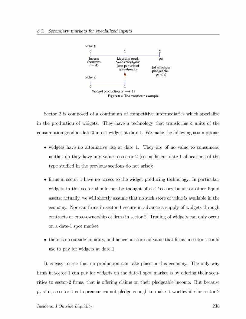
8.1. Secondary markets for specialized inputs
Sector 2 is composed of a continuum of competitive intermediaries which specialize
in the production of widgets. They have a technology that transforms c units of the
consumption good at date 0 into 1 widget at date 1. We make the following assumptions:
• widgets have no alternative use at date 1. They are of no value to consumers;neither do they have any value to sector 2 (so inefficient date-1 allocations of the
type studied in the previous sections do not arise);
• firms in sector 1 have no access to the widget-producing technology. In particular,widgets in this sector should not be thought of as Treasury bonds or other liquid
assets; actually, we will shortly assume that no such store of value is available in the
economy. Nor can firms in sector 1 secure in advance a supply of widgets through
contracts or cross-ownership of firms in sector 2. Trading of widgets can only occur
on a date-1 spot market;
• there is no outside liquidity, and hence no stores of value that firms in sector 1 coulduse to pay for widgets at date 1.
It is easy to see that no production can take place in this economy. The only way
firms in sector 1 can pay for widgets on the date-1 spot market is by offering their secu-
rities to sector-2 firms, that is offering claims on their pledgeable income. But because
ρ0 < c, a sector-1 entrepreneur cannot pledge enough to make it worthwhile for sector-2
Inside and Outside Liquidity 238
8.1. Secondary markets for specialized inputs
entrepreneurs to invest. In the anticipated absence of widgets, sector-1 entrepreneurs do
not invest either. Yet, investment is desirable (and would occur if the two sectors could
coordinate their plans at date 0) as long as ρ1 > 1+ c.
Compare this with the case where firms can coordinate plans. The consolidated net
present value for the economy is (ρ1 − 1− c) I. Assuming that firms in sector 1 are not
constrained by their date-0 endowment, the representative firm in sector 1 invests I, where
(1+ c)I−A = ρ0I , or I =A
1+ c− ρ0.
It finances the date-0 investment in widgets by issuing claims on its future income and
by transferring date-0 endowment so as to make up for the shortfall (c− ρ0)I.
Note that the coordination failure highlighted here — the failure to contract at date
0 — differs from the standard, multiple-equilibrium coordination failure developed in the
literature on strategic complementarities — e.g., Hart (1980). In our example there is only
one equilibrium. Relatedly, if ρ0 were greater than c, the problem we have identified
would be moot, but the standard coordination failure — a bad equilibrium in which sector
1 does not invest because it anticipates that sector 2 will not invest, and conversely —
could still arise.
Policy. If date-0 contracting proves infeasible, the creation at date 0 of outside liquidity
(stores of value) that can be hoarded by firms in sector 1 and traded at date 1 against the
widgets produced by sector 2 improves welfare provided that the standard coordination
failure is avoided: firms in sector 2 invest in widgets at date 0 if they expect firms in
sector 1 to invest in liquid assets and make up for the income shortfall c − ρ0 per unit;
and conversely.
A possible interpretation. The logic of our example can be used to illustrate a key distinc-
tion between intermediated and direct finance. A large theoretical and empirical literature
emphasizes the need for firms with serious agency problems to resort to costly monitoring
by intermediaries as a way to alleviate the agency problem and to create more pledgeable
Inside and Outside Liquidity 239
8.1. Secondary markets for specialized inputs
income (see, for instance, Diamond, 1984, Gorton and Winton, 2003 and Holmström and
Tirole, 1997) Firms with low agency costs, in contrast, have direct access to (cheaper)
market finance. In this context, the situation depicted in Figure 8.2 can be given the
following interpretation: At date 1, firms may face a shock that aggravates the agency
problem. For example, new opportunities for misbehavior appear, or, due to bad news, the
entrepreneur’s stake in the firm has decreased, making her more prone to waste resources
or to gamble for resurrection. Continuation then calls for monitoring by intermediaries.
Monitoring at date 1, however, requires that intermediaries hoard resources (“widgets”)
at date 0: they must build human capital (c then represents the cost of dedicating per-
sonnel that is specialized in sector 1). But, as we have just argued, intermediaries will
not have the incentive to invest in monitoring expertise, because firms lack pledgeable
income with which to pay for intermediary services at date 1 (we are assuming here that
firms cannot arrange for intermediary services in advance, in the same way that sector-1
entrepreneurs could not contract in advance with sector-2 producers of widgets in the
more formal treatment above).7
The assumption that no production can take place in the absence of monitoring (our
interpretation of widgets) is a bit stark. More generally, one could follow Holmström and
Tirole (1997) and assume that monitoring reduces moral hazard and thereby increases
pledgeable income. Consider the extreme case in which nothing is pledgeable in the absence
of monitoring. Then, the entrepreneurs in sector 1 can invest I = A in the absence of
monitoring and I = A/(1+ c−ρ0) with monitoring and coordination. But if a firm waits
until date 1 to secure monitoring, it can invest only I = A since, as we have seen, at that
point it is unable to pay monitors enough to induce them to invest at date 0.
7This interpretation points to a difficulty one is likely to encounter when trying to measure aggregate
liquidity in an industry or a country. Here, liquidity is provided by the stock of knowledge held by
intermediaries about the industry (or in the context of international crises, by the foreign financial
institutions about the country’s firms and markets), as well as by their own financial strength. Such
variables are by no means easy to measure.
Inside and Outside Liquidity 240
8.2. Application to uncoordinated international liquidity provision
8.2 Application to uncoordinated international liq-
uidity provision
8.2.1 Framework and the coordinated benchmark
Let us first briefly recall the international liquidity model of Chapter 6.
• Goods and preferences.There are two kinds of goods:
— Tradable goods, which are consumed by foreigners as well as domestic residents.
These goods will at times be called dollar goods or simply dollars.
— Nontradable goods,which only domestic residents consume. These goods are called
peso goods or pesos.
All variables referring to dollars have superscript “$ ”, while those without superscript
refer to pesos.
There are three periods, t = 0, 1, 2. We assume that economic agents only care about
the sum of their consumptions at the three dates, and therefore demand a zero expected
rate of return on investments. We further assume, mainly for convenience, that domestic
residents view tradables and nontradables as perfect substitutes. Thus, a foreigner’s utility
from the consumption stream©c$tªt=0,1,2
is
2Xt=0
c$t ,
while a domestic resident’s utility from the consumption stream©¡c$t , ct
¢ªt=0,1,2
is
2Xt=0
£c$t + ct
¤.
We use date-0 pesos as our numéraire.
All uncertainty is revealed at date 1.
Inside and Outside Liquidity 241
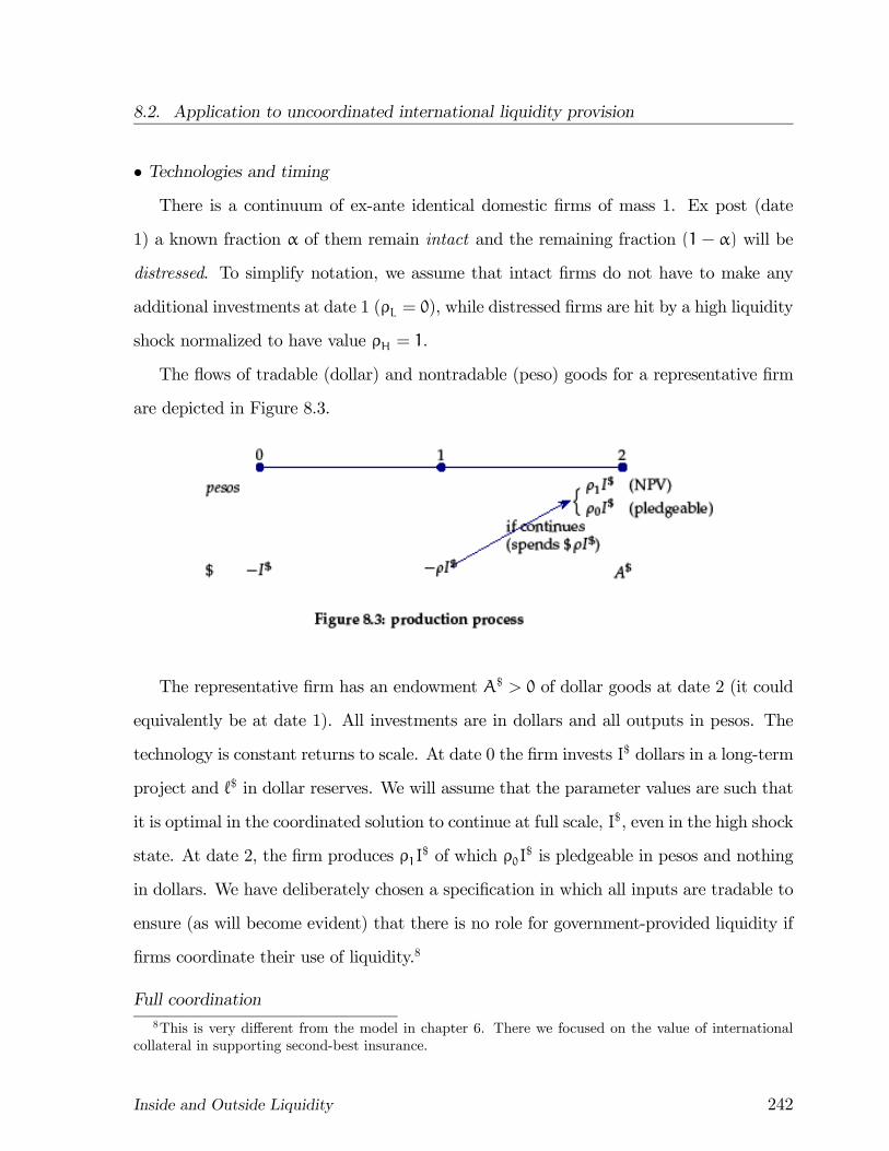
8.2. Application to uncoordinated international liquidity provision
• Technologies and timingThere is a continuum of ex-ante identical domestic firms of mass 1. Ex post (date
1) a known fraction α of them remain intact and the remaining fraction (1 − α) will be
distressed. To simplify notation, we assume that intact firms do not have to make any
additional investments at date 1 (ρL = 0), while distressed firms are hit by a high liquidity
shock normalized to have value ρH = 1.
The flows of tradable (dollar) and nontradable (peso) goods for a representative firm
are depicted in Figure 8.3.
The representative firm has an endowment A$ > 0 of dollar goods at date 2 (it could
equivalently be at date 1). All investments are in dollars and all outputs in pesos. The
technology is constant returns to scale. At date 0 the firm invests I$ dollars in a long-term
project and `$ in dollar reserves. We will assume that the parameter values are such that
it is optimal in the coordinated solution to continue at full scale, I$, even in the high shock
state. At date 2, the firm produces ρ1I$ of which ρ0I
$ is pledgeable in pesos and nothing
in dollars. We have deliberately chosen a specification in which all inputs are tradable to
ensure (as will become evident) that there is no role for government-provided liquidity if
firms coordinate their use of liquidity.8
Full coordination
8This is very different from the model in chapter 6. There we focused on the value of international
collateral in supporting second-best insurance.
Inside and Outside Liquidity 242
8.2. Application to uncoordinated international liquidity provision
As a benchmark, let us first calculate the fully coordinated solution. Since shocks are
idiosyncratic, date-1 aggregate demand for liquidity is deterministic. Given our special
assumptions ρL = 0 and ρH = 1, the aggregate demand is `$ = (1−α)I$, if firms want to
continue at full scale. Foreigners must be paid in dollars. The only source of dollars is the
representative firm’s initial endowment A$, which is split between the initial investment
and reinvestment. The budget constraint is
I$ + (1− α)I$ = A$, (8.25)
implying that
I$ =A$
1+ (1− α). (8.26)
The representative firm’s gross utility, if it holds enough reserves to cover the high
liquidity shock, is
Ug =ρ12− α
A$.
The policy of holding no reserves would yield investment I$ = A$ and a net present value
Ug = αρ1A$. Assuming that 1 > α(2− α), so that it is optimal to hoard reserves.
To meet the high liquidity shock, the corporate sector must have (1− α)I$ dollars at
date 1 and find a way to dispatch liquidity to those firms hit by the high shock. As in
the previous chapter, we assume that institutions for coordinating liquidity use are not
available.9 Instead, liquidity will be allocated in a spot market at date 1.10
8.2.2 No coordination: A date-1 spot market
When firms act on their own without any advance agreements on how liquidity is to be
used, the date-1 spot market determines how excess dollar reserves get reallocated. The
market is similar to the spot market for liquidity in section 8.1. Intact firms can do one
9Note that even if there is only aggregate risk, so that all firms are hit by the same shock, the second-
best solution is the same as for the idiosyncratic case discussed above. However, international investors
may find it easier to insure country shocks, since these are more readily identified. If foreign investors
can insure country shocks, there is no need for firms to coordinate their liquidity purchases.10Because there is no aggregate uncertainty, there is no need for state-contingent government bonds.
Inside and Outside Liquidity 243
8.2. Application to uncoordinated international liquidity provision
of two things. They can hand over their dollar reserves to distressed firms in exchange for
date-2 peso goods (paid out of the ρ0I$ income). Alternatively, they can choose to consume
their dollar reserves, which they value the same as peso goods. However, consumption is
an inferior use of dollar reserves, just like the “baseball field” was an inferior use of land
in Chapter 7. The value of consumption implies that the inferior use of dollars is worth
ρ = 1 < ρ1.
Let e1 be the date-1 real exchange rate, defined as the price of the dollar good in terms
of the peso good. The real exchange rate must fall in the range
1 ≤ e1 ≤ ρ1 (8.27)
The lower bound holds because the entrepreneurs of intact firms would prefer to consume
the tradable good if e1 fell below 1. The upper bound holds because a distressed firm
does not want to pay more for salvaging a unit of the project than what that unit can
produce at date 2.
Let us next analyze the date-1 spot market:
• Demand for dollar goods at date 1A distressed firm, holding `$ units of dollar reserves, can buy up to m$ units of dollar
goods at date 1, subject to the liquidity constraint
e1m$ ≤ ρ0(`
$ +m$). (8.28)
The left-hand side of this inequality is the total cost, expressed in peso goods, of buying
dollar goods on the spot market. The right-hand side is the amount of peso goods that
can be promised in exchange, namely the pledgeable income on salvaged assets (`$+m$).
As long as the exchange rate falls within the bounds (8.27), the demand for dollar reserves
is given by
m$ ≤ minµ
ρ0`$
e1 − ρ0, I$ − `$
¶. (8.29)
Inside and Outside Liquidity 244
8.2. Application to uncoordinated international liquidity provision
Note that the right-hand side of (8.29) is well defined, since e1 ≥ 1 > ρ0. For technological
reasons, the firm has to choose m$ so that the reinvestment scale does not exceed the
initial investment level
i$ ≡ `$ +m$ ≤ I$ ⇔m$ ≤ I$ − `$. (8.30)
• Supply of dollar goods at date 1As in section 8.1.4, intact entrepreneurs are the only agents that can rescue distressed
firms. They have dollar reserves and are willing to trade dollars for peso consumption if
the spot price is at least as high as the value of consumption. By assumption, domestic
consumers do not have dollar reserves (had they had dollar reserves at date 0, they would
have sold them to the entrepreneurs.) Foreigners do have dollars, but they are unwilling
to supply dollars for pesos, because they cannot convert peso claims into dollar goods at
date 2.
• Investment in production and in dollar reserves at date 0The date-0 gross utility of a representative firm that chooses investments I$ and `$ ≤ I$
at date 0 is11
Ug = α£ρ1I
$ + e1`$¤+ (1− α)
£ρ1(m
$ + `$)− e1m$¤
(8.31)
We have grouped the entrepreneur’s utility into two terms. The first term is the return
when the firm is intact, which happens with probability α; an intact firm produces ρ1I$
and gets e1`$ from selling (or consuming) its dollar reserves, which it does not need to
continue operations. The second term is the return when the firm is in distress, which
happens with probability 1−α; a distressed firm can salvage `$ units using its own dollar
reserves and m$ units by buying dollars in the spot market. From (8.29) we see that the
firm can purchase dollars in the amount m$ = ρ0`$/(e1 − ρ0) as long as the total does
not exceed I$ − `$.
11Note that the firm does not borrow at date 0, as (a) domestic investors cannot buy dollar goods,
(b) foreign investors can lend dollar goods, but will demand them back, a wash in terms of access to
tradables.
Inside and Outside Liquidity 245
8.2. Application to uncoordinated international liquidity provision
The entrepreneur will have to pay investments up front, because all the investments
are in dollars while all the returns are in pesos. Foreigners will not accept pesos as
payment, and domestic investors do not, by assumption, have dollars for the investments.
The entrepreneur’s date-0 budget constraint is therefore simply
I$ + `$ ≤ A$. (8.32)
• Equilibrium in the date-1 spot market
Supply must weakly exceed demand in the date-1 spot market for dollar goods, so
α`$ ≥ (1− α)m$. (8.33)
An equilibrium in the date-1 spot market is achieved when the price e1 of dollar goods
is set at a level such that when the representative firm maximizes (8.31) subject to (8.29)
and (8.32), the inequality (8.33) is satisfied and holds as an equality whenever e1 > 1. It
is easy to see that an equilibrium always exists.
At a firm optimum, the budget constraint (8.32) is always binding. Substituting
I$ = A$−`$ into the objective function (8.31) we find that the derivatives of the objective
function with respect to `$ and m$ are:
αe1 + (1− 2α)ρ1
and
(1− α)(ρ1 − e1) ≥ 0,
respectively. Note that whenever
e1 < ρ1,
the derivative with respect tom$ is positive (purchasing liquidity is cheap), so the liquidity
constraint must be binding:
(e1 − ρ0)m$ = ρ0`
$. (8.34)
Inside and Outside Liquidity 246
8.2. Application to uncoordinated international liquidity provision
Also, there would be no activity in the date-1 market if e1 were above ρ1, verifying formally
the upper bound of (8.27).
No ex-post waste of liquidity. Suppose e1 > 1. Then (8.33) is an equality as supply
must equal demand. Combining the market equilibrium condition with a binding liquidity
constraint gives the following price for the equilibrium in the date-1 dollar market:
e1 =ρ0α. (8.35)
This equilibrium price prevails, provided that e1 falls in the interval (8.27), that is,
1 <ρ0α< ρ1. (8.36)
Substituting (8.35) with (8.34) we see that (1−α)m$ = α`$ or equivalently thatm$ = αi
and `$ = (1− α)i$, where i$ ≡ m$ + `$ is the continuation scale of distressed firms. The
technology requires i$ ≤ I$. When we insert the expressions for `$ and m$ into the firm’s
objective function we see that it is optimal to choose i$ = I$. The representative firm’s
gross utility then becomes
Ug = ρ1I$ = ρ1(A
$ − `$).
We note in passing that when the price given by (8.35) prevails, the amount that the
intact firms make on selling dollars at date 1 equals the amount that the distressed firms
pay for the dollars, regardless of the level of continuation investment i$. This is, of course,
always the case in equilibrium if all the dollars get transferred from intact to distressed
firms. Because `$ = (1 − α)I$, the equilibrium allocation coincides with the second-best
allocation, in analogy with the analysis in section 8.1.2. There is no waste of dollars.
The price given by (8.35) has to fall within the bounds defined by (8.36). For α
≤ ρ0/ρ1, the date-1 price is at its upper bound
e1 = ρ1.
In this region
Ug = αρ1A$ + (1− α)ρ1`
$,
Inside and Outside Liquidity 247
8.2. Application to uncoordinated international liquidity provision
where `$ is determined by the liquidity and budget constraints after substituting I$ =
A$ − `$. The representative firm’s utility is
Ug =ρ1A
$
2− α.
Also in this case the uncoordinated solution coincides with the coordinated solution.
Ex-post waste of liquidity. We finally consider the case where the equilibrium occurs on
the boundary e1 = 1, in which case some dollar reserves will be consumed rather than
transferred to salvage distressed assets. For α > ρ0, the exchange rate given by (8.35) lies
below 1 so we must have
e1 = 1.
In this price regime it can be optimal for firms not to buy any liquidity at all at date 0.
This happens if α is high enough and the pledgeable income low. If firms do buy liquidity,
supply will exceed demand:
α`$ > (1− α)m$.
The excess supply of liquidity is consumed by the intact entrepreneurs, who are indifferent
between selling into the market and consuming when e1 = 1. Putting liquidity to an
inferior, alternative use is, of course, wasteful from a social perspective. Note, however,
that distressed firms will be able to continue at full scale. Knowing that they cannot
afford to buy much in the market (despite the price being as low as it can go), they hoard
more liquidity at date 0. In the limit, as ρ0 goes to zero, and distressed firms have no
purchasing power at date 1, the situation will be the same as in autarky — either firms
hoard `$ = A$/2 of liquidity or they do not buy any. When the distressed firms have a
bit of purchasing power (ρ0 > 0) they can reduce `$ a bit.
It is tedious, but straightforward to determine when firms opt to buy liquidity and
when they do not. The optimum either occurs at the intersection of the budget and the
liquidity constraint or at the origin. We have
Inside and Outside Liquidity 248
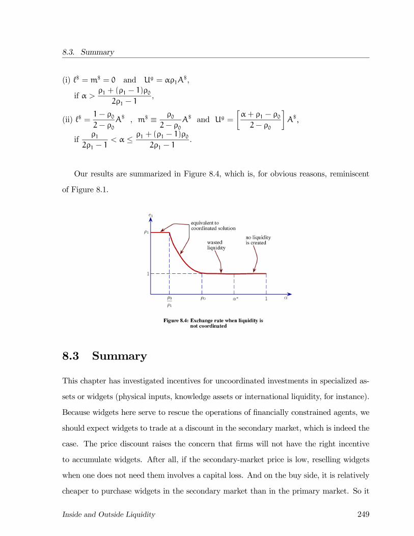
8.3. Summary
(i) `$ =m$ = 0 and Ug = αρ1A$,
if α >ρ1 + (ρ1 − 1)ρ0
2ρ1 − 1,
(ii) `$ =1− ρ02− ρ0
A$ , m$ ≡ ρ02− ρ0
A$ and Ug =
∙α+ ρ1 − ρ02− ρ0
¸A$,
ifρ1
2ρ1 − 1< α ≤ ρ1 + (ρ1 − 1)ρ0
2ρ1 − 1.
Our results are summarized in Figure 8.4, which is, for obvious reasons, reminiscent
of Figure 8.1.
8.3 Summary
This chapter has investigated incentives for uncoordinated investments in specialized as-
sets or widgets (physical inputs, knowledge assets or international liquidity, for instance).
Because widgets here serve to rescue the operations of financially constrained agents, we
should expect widgets to trade at a discount in the secondary market, which is indeed the
case. The price discount raises the concern that firms will not have the right incentive
to accumulate widgets. After all, if the secondary-market price is low, reselling widgets
when one does not need them involves a capital loss. And on the buy side, it is relatively
cheaper to purchase widgets in the secondary market than in the primary market. So it
Inside and Outside Liquidity 249
8.3. Summary
would seem that a low resale price would lead to undersupply of widgets relative to the
social optimum, a key conclusion in Caballero and Krishnamurthy (2001). The surprising
result in this chapter is that this need not be the case when firms are ex ante identical
and the only imperfection is their inability to coordinate in advance the purchase and use
of liquidity
While it is correct that a low price discourages the hoarding of widgets, this reason-
ing misses another effect: In the absence of alternative stores of value (say, Treasury
bonds), hoarding widgets provides date-1 funding liquidity (the ability to dilute the ini-
tial investors — with their ex ante consent — by issuing new securities). This relaxes the
liquidity constraint and creates an additional incentive to hoard widgets as a store of
value. The incentive is higher, the lower the secondary-market price and in our model
the incentive to hoard widgets is in the end socially optimal. The only situation where
self-provision of widgets does not replicate the coordinated outcome is when the distressed
firms have so little aggregate purchasing power that some of the widgets will be turned
into the alternative use. In this case, there is nothing the government can do to improve
welfare.
One reason why we get efficiency while Caballero and Krishnamurthy (2001) conclude
that investment in liquidity (investment in dollars, to be more specific) is suboptimal,
is that our investors have more commitment power. In particular, our investors allow
firms to issue new shares when liquidity is needed. Because intact firms have no use for
additional funds, this right will not be abused. One can argue that it would be more
realistic to assume that intact firms would abuse the right to dilute initial shareholders
(as in Appendix 2.1 of Chapter 2 and in Caballero and Krishnamurthy, 2001). On the
other hand, our analysis, when juxtaposed with Caballero and Krishnamurthy’s analysis,
identifies the inability to control the firms’ use of funds as a key assumption in their
underinvestment result.
Underinvestment occurs, perhaps more naturally, when there is a separation between
Inside and Outside Liquidity 250
8.3. Summary
the producers of widgets and the users of widgets as suggested by the asymmetric case
discussed in section 8.1.4. The shortage of pledgeable income of the buyers of widgets
discourages the sellers from investing in widgets as in the intuitive reasoning above. The
extra effect on funding liquidity is missing. In the case there is scope for policy inter-
vention; in particular, the creation of stores of value makes it possible for the buyers of
widgets to pay a high enough price to sellers thanks to higher savings.
The inquiry set forth in this chapter is still rather tentative. In particular, while
it has delivered some new insights into policy intervention, it has not delivered clear
guidelines. Furthermore, it has not investigated whether the reasons leading to the absence
of forward markets could interact with the overall logic of this argument. Our analysis
should therefore be read with caution when it comes to drawing policy recommendations.
Inside and Outside Liquidity 251

Part V
EPILOGUE
252
Summary and concluding thoughts
on the subprime crisis.
We started our research on liquidity over fifteen years ago with the aim of understanding
liquidity (collateral) shortages in financial crises.12 We close this book with some reflec-
tions on what our approach can tell us about the on-going subprime crisis. We begin
by summarizing the key themes and insights of the book, before getting into the crisis
itself.13
The main ingredients and insights
Our approach is based on two key premises. The first is that income streams are
not fully pledgeable. Only part of the pie that a firm creates can be credibly pledged to
investors,14 and consumers cannot pledge any of their future income without collateral or
through government taxation.15 The second premise is that arbitrary, state-contingent
contracts can be written on pledgeable income as in the standard Arrow-Debreu general
equilibrium model. The critical departure from the Arrow-Debreu model is therefore
the first assumption that there is a wedge between total income and pledgeable income.
Introducing a wedge extends the standard complete market model to a slightly more
12We were inspired by the severe financial crises in Scandinavia in 1991-92 and later in Asia in 1997.13The terms pledgeable income, liquidity and collateral are used interchangably in this book, including
this epilogue.14Because firms will have to give up some of the income to management, workers and monitors (e.g.
venture capitalists), who share in the rents created by firms; how much depends on many factors that we
lump together into an unpledgeable share of the pie.15This modeling assumption is a caricature of reality, of course. Unsecured consumer debt in the form
of credit cards, for instance, is not trivial, but still relatively small in comparison with collateralized debt,
such as housing.
253
realistic setting with surprisingly powerful implications.16
The first implication is that firms and financial institutions will have a demand for
liquidity despite everyone being risk neutral. In contrast to the Arrow-Debreu model,
where firms can fund all positive net present value projects on a pay-as-you-go basis, in
our model firms have to arrange funding in advance to avoid credit rationing in states
where their pledgeable income is insufficient to fund desirable continuation investments.
The firms’ demand for liquidity is a demand for insurance against future credit rationing.
With a limited net worth, the firm has to choose how much of its capital to spend on
insurance (contingent liquidity) and how much on current investment. The trade-off
results in the firm being credit rationed both today and in the future. In general, the firm
will only buy partial insurance.
A second implication of partial pledgeability of income is that it reduces the supply
of liquidity. Investors (or financial institutions) need collateral to back up their promises
for future funding of firms. If the corporate sector’s pledgeable income in some state
is too small, there will be a shortage of aggregate (inside) liquidity in that state. It is
the potential for aggregate liquidity shortages and their consequences for liquidity premia,
investment decisions, and government policies that constitute the central andmost original
part of our analysis.
If the private sector is a net lender, or if it is subject to significant aggregate shocks,
there is always insufficient inside liquidity. On the other hand, when the private sector
is a net borrower and shocks are idiosyncratic, then the private sector is self-sufficient.
Nonetheless, the second-best solution requires state-contingent insurance that transfers
liquidity from the intact to the distressed firms in an efficient way. Firm-specific credit
lines offered by a financial intermediary that holds a well-diversified market portfolio of
securities can achieve the required reallocation of liquidity, as can a variety of other state-
16We still refer to our model as one with complete markets, because the market is complete with respect
to the pledgeable income.
Inside and Outside Liquidity 254
contingent mechanisms, including the option that firms themselves hold claims in the
market portfolio.
In states where there is a shortage of aggregate liquidity, there is a liquidity premium
on its supply. The price of liquidity and the value of assets can be determined using a
liquidity asset pricing model (LAPM). The value of an asset has two components: the
consumption value of its cash flow plus the value (or cost) of the collateral that it produces
or requires as part of its investment plan. We study asset pricing using techniques familiar
from standard general equilibriummodels. We find that the equilibrium is efficient subject
to the constraint that all contracts must be secured by pledgeable income.
The government can play a key role in making up for aggregate liquidity shortages.
Its unique access to current and future consumer income through taxation, allows it to
act as an intermediary between consumers and firms. It can raise welfare by transferring
liquidity from consumers (current and future) to firms in states where the value of such
transfers is higher than the shadow cost of public funds. The marginal value of government
transfers can be inferred from the state-contingent prices for liquidity in LAPM.
In practice, the government supplies contingent liquidity through a variety of policies
and interventions including the conduct of monetary policy, the provision of deposit in-
surance, the occasional bailout of commercial banks, investment banks, pension funds and
other financial institutions (like Freddie Mac and Fannie Mae). In addition, a whole range
of social insurance programs such as unemployment insurance and social security and of
implicit catastrophe insurance (earthquakes, nuclear accidents,..) play an important role
in influencing the amount of aggregate liquidity in the economy.
It is important to stress that government transfers can be seen as part of an explicit
or implicit insurance plan. Having tax payers get involved, because private insurance
is constrained by limits on aggregate liquidity makes perfect sense, at least in theory.
Relatedly, the government also enjoys an advantage over private parties because it can
supply liquidity on a contingent basis. The private sector has to decide ex ante how
Inside and Outside Liquidity 255
much liquidity it creates, often by making investments in short-term, physical assets
(or just biasing investments in the direction of income that is more readily pledgeable).
In contrast, the government can supply liquidity once the need has materialized, saving
significantly on the cost of investing in lower-yielding projects. This implies that the state
has a particularly strong comparative advantage in offering insurance against unlikely and
extreme shocks hitting the economy.
International markets can alleviate domestic liquidity shortages, but even if there is
more than enough international liquidity to meet the needs of a country, this will not in
general eliminate the country’s liquidity shortages. A country has its own pledgeability
limitations: Non-tradable output, while exchangeable in markets with tradable goods,
must in the end go to domestic consumers and therefore has little appeal to international
investors as such. When there is a shortage of international liquidity (tradable output),
domestic liquidity supply and liquidity management by the government remain effective
just as in a closed economy.
Assuming that contingent claims markets are complete, is of course unrealistic. But
in return it offers simplicity and discipline. It also provides an upper bound on the sup-
ply of aggregate liquidity. When markets are incomplete, aggregate liquidity shortages
tend to become accentuated, as coordination problems prevent the efficient use of avail-
able liquidity. The burgeoning literature on financial crises employs almost exclusively
incomplete market models. By way of illustration, we studied a few models of this sort in
part IV of the book. We found that despite market incompleteness, the equilibrium can
sometimes be efficient, replicating the outcome of complete contingent markets. When
the equilibrium is inefficient it may exhibit:
• over-hoarding of liquidity before a crisis, because firms invest in liquidity to be ableto compete for distressed assets in the future,
• insufficient transfers of liquidity during the crisis to firms whose management cannotbe replaced (due to specific knowledge) as firms with excess liquidity prefer to invest in
Inside and Outside Liquidity 256
low-productivity projects rather than in firms that need liquidity, but do not have enough
funds to compete for them,
• consumer savings behavior that is too short-termist when consumers are employeesof firms,
• fire-sale prices that inhibit an efficient transfer of assets,
• possible under-hoarding of liquidity relative to the complete contingent market case;however, forcing firms to invest more in liquidity may not solve the problem, if the extra
reserves can be put to alternative, inferior use (because the spot price is low).
Relating our model to the subprime crisis
Our understanding of the causes of the subprime crisis is still limited. While it is
easy to list a variety of factors that must have played some part in the collapse, there
is still disagreement on the major drivers. We will focus on four factors that seem to us
particularly central and which form a relatively coherent view of the crisis. These are: (i)
the global imbalances and the savings glut, (ii) the growth of the U.S. shadow banking
system in response to the savings glut, (iii) the collapse of the wholesale funding market
that supported shadow banking, and (iv) regulatory deficiencies17.
The savings glut. There is wide-spread agreement that the increasingly large current
account deficits that the U.S. ran up in the new millennium (growing steadily from 4.4
per cent of GDP in 2000 to 6.2 per cent in 2006) were a major cause of the crisis. Why
did the account deficits grow so large? The traditional argument would suggest that the
U.S. lived beyond its means, needing ever more funds to support its consumption habits.
But there is an alternative view, originally put forward by Ben Bernanke, the current
chairman of the Federal Reserve. In a widely noticed speech in 2005, he suggested that
the problem stemmed from a global savings glut, caused largely, but not exclusively, by
17Our interpretation of events draws on Adrian and Shin (2008), Caballero et al (2008), Hellwig (2009),
Holmström (2008), Gorton (2008, 2009), chapter 3 in Gylfasson et al, (2010), and Dewatripont et al
(2010), among others.
Inside and Outside Liquidity 257
excess savings in the emerging markets of Asia. Foreign investors were looking for a safe
place to park their excess funds and found it in the U.S. The view that money was pushing
its way into the U.S. rather than being pulled in by a demand for capital, has received
wider acceptance lately. One argument in its favor is that interest rates kept falling as
the U.S. current account deficit grew. This seems inconsistent with the notion that the
U.S. consumer was driving the growth.18
The notion that Asian money was looking for safe investment opportunities in the
U.S., fits well with our basic premise that a country can have a shortage of aggregate
liquidity if pledgeable income is low. In developing economies, poorly developed financial
markets and political and legal uncertainties generally make the pledgeable income of
firms small. Paired with exceptionally high savings ratios, this may well have caused
much of the savings to be channeled towards countries with higher fractions of pledgeable
income and greater safety19.
The savings glut also may have made it easier for the housing bubble to emerge.20
Bubbles augment the stock of stores of value, albeit in a very imperfect way to the extent
that that they are an unreliable method of carrying income over from one period to the
next. They risk bursting, and what is worse, they burst at the wrong time for those
institutions that seek liquidity from the bubble: When a bubble bursts, not only does
18See Caballero, Farhi and Gourinchas (2008). However, Taylor (2009) has argued forcefully that global
imbalances played a minor role relative to U.S. monetary policy, which was too lax, keeping interest rates
low for too long.19These observations fit well with Forbes (2010)’s empirical demonstration that foreigners hold greater
shares of their investment portfolios in the US if they have less developed financial markets. She further
shows that foreigners, who invested $6.2 trillion between 202 and 2006 earned substantially lower returns
on their US investments than US investors earned abroad; and that diversification motives do little to
explain the patterns of foreign investments in the US.20There is always some difficulty in identifying empirically the existence of a bubble. Take the recent
bubble in real estate in the United States. It could be argued that the very large subsidies to house
ownership (both direct- such as the tax deductibility of interest- and indirect- for instance, low interest
rates, the lenient regulatory treatment of asset backed securities or the implicit insurance given to Freddie
Mac and Fannie May) made the fundamentals of real estate very strong if these subsidies were expected to
last. See however Shiller (2008) for a rather convincing case for the existence of a bubble. For important
historical perspectives on bubbles and financial crises, see Kindelberger (1989) and Reinhart and Rogoff
(2009).
Inside and Outside Liquidity 258
it have a negative effect on these institutions’ solvency (a wealth effect), it also deprives
them of collateral at a moment when it is most valuable (because when liquidity becomes
scarcer, interest rates fall, and leveraging one’s collateral becomes more attractive).21
The rise of shadow banking. Global imbalances, as such, do not explain why the
bulk of excess savings flowed into the U.S. rather than into Europe, for instance.22 One
reason could be the U.S. consumer’s willingness to go deep into debt, especially in the
low interest rate environment maintained by the Fed at the time. Another possibility is
that the U.S. was especially well positioned to absorb the global savings glut because its
financial markets were (and still are) the most advanced in the world. In particular, the
U.S. had come up with a financial innovation that enabled it to absorb huge inflows of
capital in a short period of time — the shadow banking system.
The shadow banking system is usually defined as that part of banking (intermediation
of credit) that is not explicitly insured by the government.23 It is comprised of a network
of players — investment banks, hedge funds, money market mutual funds (MMMF) and
Government Sponsored Entities (GSEs) like Freddie Mac and Fannie Mae among others
— all helping to intermediate credit through the market. The shadow banking system is
based on wholesale funding rather than deposits, making it potentially more vulnerable
to runs.
The liabilities of the shadow banks grew rapidly from less than 10 per cent of total
bank liabilities in 1980 to about 60 per cent in 2008.24 The growth rate was especially
strong after 1995. It is suggestive that the yearly growth of gross liabilities was of the
same order of magnitude as the yearly U.S. trade deficits. Shadow banks must have played
a central role in channeling the vast amounts of money that flowed into the U.S.
21See Farhi-Tirole (2009a). Other recent work on bubbles includes Kocherlakota (2009) and Ventura
(2010); the latter argues that bubbles can substitute for imperfect capital flows and then appear in
countries in which productivity is low relative to the rest of the world.22In fact, the European private sector invested substantial amounts in the U.S.during the same period.23See Potzar et al (2010).24Figure 1 in Potzar et al (2010).
Inside and Outside Liquidity 259
The shadow banking system has been widely implicated in the crisis. Many see the
whole system as a scam, driven by excessive short-term incentives for bankers on Wall
Street. Some of these accusations are certainly valid. But the original driver of the
growth of shadow banking must in the first instance have been its ability to respond to
the demand for safe investment opportunities. In particular, the repo market, which is at
the core of shadow banking, offered a form of secured lending that emulated many of the
features of demand deposits in commercial banking.
To understand how, let us briefly discuss the repo market. A repo (repurchase agree-
ment) consists of two simultaneous transactions. In the first, party A buys a security
(almost always debt) from party B at a price that typically is below the value of the
security (the difference is called the "haircut"). In the second transaction, party B agrees
to buy back the security for a slightly higher price at a later date (the next day, in case
of an overnight repo). By rolling over an overnight repo until one or the other party
withdraws, the repo becomes similar to a deposit. If party A decides not to roll over an
overnight repo, the effect is the same as the withdrawal of the deposit. However, unlike
traditional banking, the repo market was designed to secure hugely bigger deposits. —
typically millions or even hundreds of millions of dollars in a single trade. Federal deposit
insurance would provide minimal protection for investments of this size, whereas the repo
market, by selling a security in exchange for the deposit, could provide insurance on the
appropriate scale. There is a key legal detail in the repo contract: If party B (the bor-
rower) cannot repurchase a security when party A (the investor) demands it (i.e. pay
back A’s deposit), party A owns the security and is immediately free to sell it or use it as
collateral in another repo transaction. Structuring things as a purchase and repurchase
agreement is ingenious, because it avoids having a multi-million dollar deposit tied up in
a bankruptcy process if party B defaults. Unlike traditional banking, repo markets were
highly scaleable without much (apparent) risk. The only limitation, really, was the supply
of securities and the assets underlying them.
Inside and Outside Liquidity 260
The raw material for creating new securities came mostly from housing. There are
several reasons for this. Housing is by far the largest consumer asset. But before the era
of modern financial engineering, housing was an underdeveloped asset. Keeping mort-
gages on the books of regional banks was like operating a severely under-utilized financial
parking lot: mortgages that could serve as collateral for millions of investors with billions
more money, were serving just a fraction of the potential investor demand. And American
home owners that had paid off their loans were denying foreign investors the opportunity
to park their money in such houses with minimal risk. The enormous growth of home eq-
uity loans in the 1990s, unleashed some of the housing potential. Securitization, especially
of mortgages, but later on of just about any other kind of asset (car loans, student loans,
credit card loans, etc) made the most of this opportunity. Securitization could deliver
highly rated (AAA) bonds out of relatively marginal assets using tranching.25 The com-
bination of the repo market with asset-backed, highly rated securities used to secure repo
trades, created a formidable intermediation machine, one that in appearance no other
country could match in terms of legal safety and capacity.
How does securitization and shadow banking fit our theory? A plausible interpretation
is that the shadow banking system strived to and perhaps came close to replicating the
state-contingent use of collateral that is the central ingredient in our model (see chapter
4). By mixing securities to create portfolios that diversified away much of the idiosyncratic
risk, parties were left trading aggregate risk. Relatively liquid markets in such risk made it
possible to use state-contingent aggregate liquidity more efficiently as the theory suggests
one should. In this view, securitization created investment instruments that used collateral
much more effectively than if the funds had been parked for long periods in non-traded
25The creation of structured products involves two steps: first, pooling of assets (e.g. mortgages) and
second, issuing of claims against these assets — mainly debt — with varying credit ratings. The second
step is tranching. Gorton (2008, 2010) describes in detail how structured products are created. Coval
et al (2009) contains an excellent analysis of how much AAA-rated securities can be created from low
subprime mortgages, depending on the correlation of the underlying assets.
Inside and Outside Liquidity 261
instruments.26
The tri-party repo system, which is a major part of the repo market, illustrates the
contingent use of aggregate liquidity.27 Each day, the dealers (borrowers) in the tri-
party repo market place collateral (securities) with the clearing banks. The clearing
banks provide a number of services, including daily optimization of the allocation (and re-
allocation) of a dealer’s collateral to its investors. There are only two banks, JP Morgan
Chase and Bank of New York Mellon, which act as clearing banks for tri-party repos,
possibly because economies of scale are critical for the allocation of collateral. Bilateral,
over-the-counter repos do not offer the same matching efficiencies. The same trades
that are made bilaterally can be made by tri-party repos, but bilateral repos have to be
cleared sequentially, so collateral cannot be optimized at the end of the day.28 Intraday
large payment systems, such as the Clearing House Inter-Bank Payment System (CHIPS)
the main privately held clearing house for large-value transactions in the United States,
similarly are designed to make efficient use of limited collateral while concurrently trying
to contain systemic risk .29
To sum up, the financial innovations that have been so decried lately should in principle
have raised welfare by allowing a much better use of collateral in the economy; so what is
being questioned is not the ideas themselves, but how they were and can be implemented
in practice. The collateral underlying the state-contingent claims was not what it was
supposed to be. We now turn to possible explanations for this failure.
26Regulatory arbitrage was another powerful driver. By moving capital off their balance sheets, com-
mercial banks could evade onerous capital constraints. Capital charges were reduced roughly by a factor
of ten when assets were moved into Special Purpose Vehicles (SPVs).27For an in-depth analysis of tri-party repos, see the report of the Payments Risk Committee (2010).28The tri-party system is not without its problems, because the clearing banks are highly exposed
during the day, effectively providing huge bridge loans to the broker-dealers. This poses big risks for
the clearing banks, which may react abruptly and decisively to news about the credit worthiness of their
clients. By raising haircuts, or in the extreme, by refusing to roll over a bridge loan for a counter-party,
whose risk has increased (such as Lehman), they can do quickly do significant damage to the position of
broker-dealers. See Tuckman (2010).29See Rochet-Tirole (1996b) for a description of the working and properties of intraday payment sys-
tems.
Inside and Outside Liquidity 262
The panic. We now know that the reliance on wholesale funding, especially the in-
creasing fraction of overnight lending in the shadow banking system, proved much riskier
than investors had imagined. In August 2007, the market for asset-backed commercial
paper (ABCP) collapsed.30 While the ABCP market was not big enough to set off a
panic, the collapse elevated the level of risk as measured by Libor-OIS spreads, for in-
stance. The much larger repo market, mostly secured by AAA-rated products, initially
held up, though haircuts increased and the terms of funding became shorter. But when
Lehman fell, in September 2008, the myth of repos as secure deposit-like contracts un-
raveled. Markets for asset-backed securities, which had been very liquid, froze quickly as
banks began to question not just the underlying value of mortgage-backed securities but,
more importantly, the counter-party risks caused by impaired mortgage-backed assets. A
full-blown panic ensued.
It is difficult to judge whether the bond ratings were flawed from an ex-ante perspective
or whether investors were hit by a highly unlikely tail event. Given that many people were
concerned about the real estate bubble bursting at some point too little attention was
paid to the consequences of an aggregate shock in the housing market that could bring
down the value of assets across the nation. That said, a drop in the average nominal
price of U.S. housing had not occurred since the Great Depression, making it difficult
to assess aggregate risks and forecast a 30% drop in prices. Also, it is clear that the
standard mechanics of a balance sheet driven crisis — funding and margin spirals caused
by and causing fire sales of assets, flight to quality and strategic hoarding of liquidity —
all contributed to the large collapse in prices. This systemic risk, or at least its size, was
largely overlooked.
Our complete market model views the panic as an exogenous tail event; it says nothing
30See Covitz et al (2009). The ABCP market was much smaller than the repo market and ABCPs
were not tranched (only one type of claim was issued). Banks provided liquidity backstops for the ABCP
market, which also helped prevent a panic. Subsequently, such backstops contributed greatly to the
spread of the crisis into commercial banking.
Inside and Outside Liquidity 263
about how a panic might unfold, since all contracts are made at the beginning.31 How-
ever, it can explain why firms may choose not to buy insurance against rare events. In
our model, firms may cut down production dramatically (in the absence of government
assistance) when an aggregate shock hits, because liquidity is so scarce and the ex ante
returns from investing in private insurance to cover such an eventuality is low. Liquidity
could be scarce, because of adverse selection in the market for collateral; it would be easy
to incorporate this explicitly into our model, but we have not done so. Liquidity could
also be scarce in states where liquidity is very valuable (ex post), but the states are so
hard to define that the assets needed to back up the insurance have to be broad, requiring
high and costly up-front investments, as we discussed earlier in this epilogue.
The subprime crisis fits both conditions. Arguably, adverse selection, driven by un-
certainty about counter-party risks, froze many markets.32 And even if many saw the
possibility of a collapse in house prices, the fact that so few did something about it, sug-
gests that either they believed that the consequences would be relatively benign or, as we
discuss next, they deliberately gambled on the tail event. Also, buying insurance against
a catastrophic event may be hard, because there is insufficient liquidity (collateral) to
back up such insurance. From this point of view, our approach of modeling the collapse
as an exogenous event is not an unreasonable starting point for analyzing some aspects
31A large literature (e.g. Allen and Gale 2000, Caballero and Simsek 2009) shows how one bank’s default
may propagate in a financial system in which institutions are interdependent through cross-exposures
(in interbank or derivatives markets for example). The magnitude and impact of the resulting contagion
effects depend on the completeness of the structure of claims, on the existence of a common understanding
of these claims (securities traded in OTC markets can have unforeseen or complex consequences) and
on the opaqueness of bilateral exposures (as participants need to know the solvency not only of their
counterparties, but also that of their counterparties’ counterparties, and so on). While this literature
obtains a number of useful insights, cross-exposures are taken as exogenous; in particular, they are
unaffected by the regulatory environment (cf. the centralization and transparency of intra-day payment
systems — see Rochet and Tirole, 1996b, for a description — or the current regulatory push toward central
clearing houses for derivative products). Related, it is interesting to study the benefits of decentralized
systems (in Rochet and Tirole, 1996a, the benefit is associated with mutual monitoring). We are not
aware of research showing how cross-exposures and shortages in aggregate liquidity feed back on each
other, but the work of Caballero and Simsek (2009) for example suggests that fear of propagation may
lead liquidity to dry up rather quickly.32See for instance Acharya et al (2009) and Caballero and Simsek (2009).
Inside and Outside Liquidity 264
of the crisis.33
One of the key implications of our model is that there is a role for government in
redistributing wealth ex post. Transfers from taxpayers (that is, consumers) to the cor-
porate sector — including bailouts of banks, to the extent banks are the efficient channel
for such transfers — can be rationalized if the government can make pledges on behalf of
consumers (especially consumers who are not yet born). In practice such plans take a
variety of forms. A looser monetary policy lowers interest rates and transfers resources
from consumers to entrepreneurs, by lowering the cost of reinvestments and by providing
capital gains for those who own government debt (entrepreneurs buy government bonds
in our model). Also, at a conceptual level, the numerous liquidity facilities provided by
the Fed to jump start frozen asset markets in the shadow banking system (TARP, TALF,
TLGP, etc.) receive support from our model, though our model does not speak to the
relative merits of any given liquidity facility.
Regulatory weaknesses. Of course, government transfers and insurance come with well-
known costs. We considered the dead-weight losses from taxation, but did not consider the
moral hazard problems associated with subsidized insurance, especially bailouts that the
government was forced to undertake ex post. It is clear that the subprime crisis revealed
very significant weaknesses in the regulatory systems that were meant to keep in check
moral hazard and other dysfunctional actions. We have taken a normative viewpoint —
analyzing how the state should manage aggregate liquidity — rather than a positive one —
analyzing the political economy of domestic liquidity management. Our analysis therefore
misses a crucial element of the recent subprime crisis. Let us briefly mention how we could
embody the positive considerations into our analysis.
Consider first the role of the state in the traditional banking sector. One view of
33Of course, at a more detailed level, the crisis was the consequence of many factors, including the
(deliberately) complex way the securitized contracts were structured. There is every reason to try to gain
a good understanding of how the panic actually evolved. Treating the crisis as an exogenous state in the
way we do tells us nothing about this.
Inside and Outside Liquidity 265
regulation has it that the state monitors on the behalf of retail depositors, clients of
insurance companies, pension funds or MMMFs that the financial institution is adequately
capitalized and operates proper risk management processes so as not to leave the economic
agents — or the deposit insurance fund — with an empty shell .34 Yet in many countries, the
state, by ignoring off-balance sheet vehicles, by accepting (at the international level) low
capital requirements for the trading book, and by permitting (or failing to check) other
actions that circumvented capital requirements, allowed regulated institutions to over-
lever themselves. In the US, it also provided many subsidies for real estate investments,
including the indirect subsidies from Freddie Mac and Fannie Mae. Subsidies promote
excess investment, which according to our model sows the seeds for a subsequent liquidity
shortage, since financial institutions trade off how much to invest in productive assets and
how much in liquidity (insurance).
Consider next the role of the state in the shadow banking sector. Large investment
banks were largely unregulated. Yet they and their creditors felt that they could count
on a bailout with taxpayer money if the investment banks got into trouble — indeed,
the financial markets were flabbergasted when the US authorities let Lehman go under.
This implicit access to taxpayers’ money has dramatic consequences as it implies that
troubled institutions can keep refinancing and gamble for resurrection without any market
discipline. Observers sometimes point out that many wealthy managers and investors in
the shadow banking system lost their shirt and take this as evidence against the moral
hazard argument. The point, though, is that the implicit insurance of short-term funding
allowed them to gamble with taxpayer money and to continue receiving financing, when
they should have de-levered or even shut down.
But why were states eager to rescue institutions in which no small depositor had in-
vested? The answer is “systemic risk”, the fear that a default might propagate through
the financial system. The combination of interconnectedness and opaqueness of cross-
34This view is developed in more detail in Dewatripont and Tirole (1994).
Inside and Outside Liquidity 266
exposures made a default particularly troubling for the financial system, which after the
collapse of Lehman had little clue as to how subsequent episodes would unfold and there-
fore chose safety over almost any risk. The regulators were on the whole too tolerant
when they acquiesced to large exposures in opaque OTC derivative markets and thereby
accepted that regulated entities would be heavily exposed if large unregulated institu-
tions defaulted. This led to substantial additional commitments of taxpayers’ money,
which unregulated institutions took advantage of. It would have been wiser to require
that derivative contracts between regulated and unregulated institutions be traded in ex-
changes with a well-capitalized central clearing house as the counterparty. In short, the
state supplied liquidity in a way that created moral hazard. Needless to say, our theoret-
ical conclusions on the role of the state as provider of liquidity presume that liquidity is
injected in a way that limits moral hazard.
We mentioned above that repo markets may well have strived to emulate the optimal
state-contingent use of aggregate liquidity or at least significantly improved the use of the
collateral. This comment applies to orderly times in the market. The crisis suggests that
coming close to efficiency in normal times may provide no guarantees against a crisis in
exceptional times. Put differently, trading systems that emulate contracts are not as good
as contracts, when times get tough. This has been seen many times. Long Term Capital
Management collapsed because the trading strategy did not work in all states of nature.
Had there been explicit contingent contracts, perhaps LTCM would have protected itself
against the collapse. On the other hand, it is possible that it relied on a government
bailout. The same was true when all portfolio insurance strategies ran for the exits at
the same time in 1987. The programs that functioned so beautifully against idiosyncratic
risks in peaceful times, proved worthless or worse in the face of a big aggregate shock.
This raises the question of transparency of financial claims and markets and the role
of clearing houses and other financial institutions. With organized markets, there is more
transparency and better information about outstanding positions and risks (though the
Inside and Outside Liquidity 267
both the LTCM and the portfolio insurance examples suggest that parties can create
complex strategies that are completely hidden from the eyes of the market — intentions
are not easily inferred from the way people trade, especially in the case of rare events.)
However, exactly how and where transparency should be provided is not obvious. There
is a fundamental paradox embedded in liquidity provision. In order to function well,
liquidity providing markets are designed to minimize the need for information acquisition.
Debt is the dominant instrument, because it is information insensitive.35 Parties that
trade in debt that is sufficiently over-collateralized need not worry about adverse selection
stemming from private information about the underlying collateral. It is sufficient to know
that there is enough collateral. But if the purpose of debt is to provide little incentives
for information acquisition (about credit risk), it is hard to see how debt markets can
properly reflect the price of systemic risk. The suddeness with which financial crises
typically appear is consistent with lack of information about systemic risk. To remedy
the situation, the government will either have to produce such information itself (e.g.
through periodic stress tests) or come up with some way to make the markets produce
better information (e.g. by requiring trade in instruments that are more information
sensitive).
In order to understand the role of systemic risk, how it should be measured and what
types of transparency will be good for getting information about it, one has to move away
from the complete market model to a model that offers a deeper understanding of how
35Gorton and Penacchi (1990) argued that banks, by issuing riskless debt, allow depositors to avoid the
costs of adverse selection. Dang et. al. (2010) analyze a model where risky debt is optimal, because it is
least information sensitive in the sense that parties will have the lowest incentive to collect information.
For this reason, debt maximizes the amount of wealth that can be transported from one period to the
next. The paper also shows that bad news about the aggregate state of the economy (e.g. lower housing
prices) will result in write-downs of debt, sometimes exceeding the reduction in the fundamental value of
debt to prevent costly information acquisition and sometimes in adverse selection. In both instances the
reduction in trade is amplified by bad news, which is one of the manifestations of a crisis.
The transition from an information insensitive to an information sensitive security helps us understand
why trading partners were so ill informed about the complex securities they were trading before the crisis
and why they wanted to know so much more about the securities once the crisis broke out. In the logic
of the model, this is privately rational.
Inside and Outside Liquidity 268

crises erupt and what kinds of warning signs about the systemic risk one should follow.
Building the conceptual foundation for measuring systemic risk remains a challenging
task.
Inside and Outside Liquidity 269
Bibliography
[1] Acharya, V. D. Gale and T. Yorulmazer (2009), "Rollover Risk andMarket Freezes,"
working paper, Federal Reserve Bank of New York.
[2] –— and M. Richardson (2009) Restoring Financial Stability: How to Repair a Failed
System, Wiley-VCH, Hobeken, New Jersey.
[3] Adrian, T. and H. Shin (2008) “Financial Intermediaries, Financial Stability and
Monetary Policy,” in Maintaining Stability in a Changing Financial System, Pro-
ceedings of the 2008 Jackson Hole Conference, Federal Reserve Bank of Kansas
City.
[4] Aghion, P., Bolton, P., and J. Tirole (2004) “Exit Options in Corporate Finance:
Liquidity vs Incentives,” Review of Finance, 3: 327—353.
[5] Akerlof, G. (1970) “TheMarket for Lemons, Qualitative Uncertainty and theMarket
Mechanism,” Quarterly Journal of Economics, 84: 488—500.
[6] Allais, M. (1947) Economie et Intérêt, Paris: Imprimerie Nationale.
[7] Allen, F., and D. Gale (1994) “Liquidity Preference, Market Participation and Asset
Price Volatility”, American Economic Review, 84: 933—955.
[8] –— (1998) “Optimal Financial Crises,” Journal of Finance, 53:1245—1284.
[9] –— (2000) “Financial Contagion,” Journal of Political Economy, 108: 1—33.
270
[10] –— (2004) “Optimal Currency Crises,” Carnegie-Rochester Conference Series on
Public Policy, Elsevier, 53: 177-230.
[11] –— (2005) “From Cash-in-the-Market Pricing to Financial Fragility,” Journal of the
European Economic Association, 3(2-3): 535—546.
[12] –— (2007) Understanding Financial Crises, Oxford University Press.
[13] Amador, M. (2008) “Sovereign Debt and The Tragedy of the Commons,” WP Stan-
ford University.
[14] Arrow, K. (1970) Essays in the Theory of Risk Bearing, Amsterdam: North-
Holland.
[15] Attar, A., Mariotti, T., and F. Salanié (2009) “Non-Exclusive Competition in the
Market for Lemons,” forthcoming Econometrica.
[16] Bernanke, B. (2005) “The Global Savings Glut and the U.S. Cur-
rent Account Deficit,” Sandridge Lecture, Virginia Association of Eco-
nomics, Richmond, Virginia ; available on Federal Resere Board website:
http://www.federalreserve.gov/boarddocs/speeches/2005/200503102.
[17] Bernanke, B and M. Gertler (1989), "Agency Costs, Net Worth and Business Fluc-
tuations," American Economic Review, 79: 14-31.
[18] Biais, B., Mariotti, T., Plantin, G., and J.C. Rochet (2007) “Dynamic Security
Design: Convergence to Continuous Time and Asset Pricing Implications,” Review
of Economic Studies, 74(2): 345—390.
[19] Biais, B., Mariotti, T., Rochet, J.C., and S. Villeneuve (2010) “Large Risks, Limited
Liability and Dynamic Moral Hazard,” Econometrica, 78(1): 73—118.
[20] Blanchard, O. and S. Fischer (1989) Lectures on Macroeconomics, MIT Press.
Inside and Outside Liquidity 271
[21] Bolton, P., and D. Scharfstein (1990) “A Theory of Predation Based on Agency
Problems in Financial Contracting,” American Economic Review, 80: 93—106.
[22] Bolton, P., Santos, T. and J. Scheinkman (2009) “Outside and Inside Liquidity”,
mimeo, Columbia University and Princeton University.
[23] Boot, A., Thakor, A. and G. Udell (1987) “Competition, Risk Neutrality and Loan
Commitments,” Journal of Banking and Finance, 11: 449-71.
[24] Broner, F., Martin, A., and J. Ventura (2010) “Sovereign Risk and Secondary Mar-
kets,” forthcoming, American Economic Review.
[25] Brunnermeier, M., and L. Pedersen (2009) “Market Liquidity and Funding Liquid-
ity,” Review of Financial Studies, 22(6): 2201—2238.
[26] Bryant, J. (1980) “A Model of Reserves, Bank Runs, and Deposit Insurance,” Jour-
nal of Banking and Finance, 43: 749—761.
[27] Caballero, R. and A. Krishnamurthy (2001) “International and Domestic Collateral
Constraints in a Model of Emerging Market Crises,” Journal of Monetary Eco-
nomics, 48(3): 513—548.
[28] Caballero, R. and A. Krishnamurthy (2002), “A Dual Liquidity Model for Emerging
Markets,” American Economic Review Papers and Proceedings. 92(2) : 33—37.
[29] –— (2003a) “Excessive Dollar Debt: Financial Development and Underinsurance,”
Journal of Finance, 58: 867—893.
[30] –— (2003b) “Smoothing Sudden Stops,” Journal of Economic Theory 119(1): 104—
127.
[31] –—, E. Fahri and P-0. Gourinchas (2008), "An Equilibrium Model of Global Imbal-
ances and Low Interest Rates," American Economic Review, Vol 98 (1): 358—393.
Inside and Outside Liquidity 272

[32] –— and P. Kuralt (2009), "The ’Surprising’ Nature and Origins of the Financial
Crisis: A Macroeconomic Proposal," in Financial Stability and Macroeconomic Sta-
bility. Symposium sponsored by the Federal Reserve of Kansas City at Jackson Hole,
Wyoming.
[33] –— and A. Simsek (2010), "Fire Sales in a Model of Complexity," working paper,
Department of Economics, MIT.
[34] Castiglionesi, F., Feriozzi, F. and G. Lorenzoni (2010) “Financial Integration and
Liquidity Crises,” mimeo, Tilburg University and MIT.
[35] Conning, J. (2004) “Monitoring by Delegates or by Peers? Joint Liability Loans
under Moral Hazard,” working paper, Hunter College, Department of Economics.
[36] Coval, J. D., Jurek, J. and Staff ord, E. (2009): “The Economics of Structured
Finance,” Journal of Economic Perspectives, Vol 23 (1): 3—25.
[37] Covitz, D.M., N. Liang, and G.A. Suarez (2009), "The Evolution of a Financial Cri-
sis: Panic in the Asset-Backed Commercial Paper Market," Finance and Economics
Discussion Series, 2009-36, Federal Reserve Board, Washington, D.C.
[38] Daley, B., and B. Green (2010) “Waiting for News in the Market for Lemons,”
mimeo, Duke University and Northwestern University.
[39] Dang T.V., G. Gorton and B. Holmstrom (2010), "Financial Crises and the Opti-
mality of Debt for Liquidity Provision, working paper, Yale University.
[40] DeMarzo, P., and M. Fishman (2007a) “Agency and Optimal Investment Dynam-
ics,” Review of Financial Studies, 20(1): 151—188.
[41] –— (2007b) “Optimal Long-Term Financial Contracting,”Review of Financial Stud-
ies, 20(6): 2079—2128.
Inside and Outside Liquidity 273
[42] DeMarzo, P., Fishman, M., He, Z., and N. Wang (2009) “Dynamic Agency and
the q Theory of Investment,” mimeo, Stanford University, Northwestern University,
University of Chicago, Columbia Business School.
[43] De Soto, H. (2003) The Mystery of Capital: Why Capitalism Triumphs in the West
and Fails Everywhere Else. Basic Books.
[44] Dewatripont, M., and P. Bolton (2005) Contract theory, MIT Press: Cambridge and
London.
[45] Dewatripont, M., and J. Tirole (1994) The Prudential Regulation of Banks, MIT
Press.
[46] Dewatripont, M., Rochet, J.C., and J. Tirole (2010) Balancing the Banks, Princeton
University Press.
[47] Diamond, D. (1984) “Financial Intermediation and Delegated Monitoring,” Review
of Economic Studies, 51 (3): 393—414.
[48] Diamond, D. (1997) “Liquidity, Banks, and Markets,” Journal of Political Econ-
omy, 105 (5): 928—956.
[49] Diamond, D. and P. Dybvig (1983) “Bank Runs, Deposit Insurance, and Liquidity,”
Journal of Political Economy, 91: 401—19.
[50] Diamond, D. and R. Rajan (2009) “Fear of Fire Sales and the Credit Freeze,” mimeo,
University of Chicago.
[51] Diamond, P. (1965) “National Debt in a Neo-Classical Growth Model,” American
Economic Review, 55: 1126—1150.
Inside and Outside Liquidity 274
[52] Dow, G., Gorton, G., and A. Krishnamurthy (2005) “Equilibrium Asset Prices
and Investment under Imperfect Corporate Control,” American Economic Review,
95(3): 659—681.
[53] Farhi, E., and J. Tirole (2009a) “Bubbly Liquidity,” mimeo, Harvard University and
Toulouose School of Economics.
[54] –— (2009b) “Collective Moral Hazard, Maturity Mismatch and Systemic Bailouts,”
mimeo, Harvard University and TSE.
[55] Farhi, E., Golosov, M., and A. Tsyvinski (2009) “A Theory of Liquidity and Regu-
lation of Financial Intermediation,” Review of Economic Studies, 76 (3): 973—992.
[56] Faure-Grimaud, A., and D. Gromb (2004) “Public Trading and Private Incentives,”
Review of Financial Studies 17: 985—1014.
[57] Forbes, K. (2010) “Why do Foreigners Invest in the United States?" Journal of
International Economics 80(1): 3-21.
[58] Froot K.A., Scharfstein, D.A., and J.C. Stein (1993) “Risk Management: Coordi-
nating Corporate Investment and Financing Policies,” Journal of Finance, 48(5):
1629—1658.
[59] Fudenberg, D., and J. Tirole (1985) “Preemption and Rent Equalization in the
Adoption of New Technology,” Review of Economic Studies, 52: 383—402.
[60] Geanakoplos, J. (1996) “Promises Promises,” working paper, Cowles Discussion
Paper 1143, Yale University.
[61] –—, Zame, D.A., and P. Dubey (1995) “Default, Collateral, and Derivatives,”
mimeo, Cowles Foundation, Yale University.
Inside and Outside Liquidity 275
[62] Goldstein, I., and A. Pauzner (2005) “Demand-Deposit Contracts and the Proba-
bility of Bank Runs,” Journal of Finance, 60(3): 1293—1328.
[63] Gompers, P., and J. Lerner (1999) The Venture Capital Cycle. Cambridge, MA:
MIT Press.
[64] Goodhart, C. (2008) “Liquidity Risk Management,” Banque de France Financial
Stability Review, 11: 39—44.
[65] Gorton, G. (2008), “The Panic of 2007,” in Maintaining Stability in a Changing
Financial System, Proceedings of the 2008 Jackson Hole Conference, Federal Reserve
Bank of Kansas City.
[66] –— (2010) Slapped in the Face by the Invisible Hand: The Panic of 2007. Oxford
University Press.
[67] –— and G. Pennacchi (1990). "Financial Intermediaries and Liquidity Creation,"
Journal of Finance, Vol XLV (1): 49-71.
[68] –— and A. Whinton (2003) “Financial Intermediation,” in G. Constantinides, M.
Harris and R. Stultz,eds (with the help of A Whinton), Handbook of the Economics
of Finance. Amsterdam: Elsevier Publishing.
[69] Gottschalk A. O. (2008) “Net Worth and the Assets of Households: 2002,” Current
population reports, U.S. Census Bureau.
[70] Gurley, J. and E. Shaw (1960) Money in a Theory of Finance, Washington, DC:
Brookings Institution.
[71] Gylfasson, T, B. Holmström, S. Korkman, V. Vihriälä, H. Tson Söderström (2010).
Nordics in Crisis: Vulnerability and Resilience, Research Institute of the Finnish
Economy, Helsinki: Taloustieto.
Inside and Outside Liquidity 276

[72] He, Z., and A. Krishnamurthy (2009) “A Model of Capital and Crises,” working
paper, Northwestern University.
[73] Hellwig, M. (1994) “Liquidity Provision, Banking, and the Allocation of Interest
Rate Risk,” European Economic Review, 38(7):1363—1390.
[74] –— (2000) “Financial Intermediation with Risk Aversion,” Review of Economic
Studies, 67: 719—742.
[75] –— (2009) “Systemic Risk in the Financial Sector: An Analysis of the Subprime-
Mortgage Financial Crisis,” De Economist, 157: 129—207.
[76] Hicks, J. (1967) Critical Essays in Monetary Theory, Oxford: Oxford University
Press.
[77] Holmström, B. (2008) “Comment on ‘The Panic of 2008’ by Gary Gorton,” in
Maintaining Stability in a Changing Financial System. Symposium sponsored by
The Federal Reserve Bank of Kansas City at Jackson Hole, Wyoming, 2008.
[78] Holmström B. and J. Tirole (1996) “Modelling Aggregate Liquidity,” American
Economic Review, Papers and Proceedings, 86: 187—191.
[79] –— (1997) “Financial Intermediation, Loanable Funds, and the Real Sector,” Quar-
terly Journal of Economics, 112: 663—692.
[80] –— (1998) “Private and Public Supply of Liquidity,” Journal of Political Economy,
106: 1—40.
[81] –— (2000) “Liquidity and Risk Management,” Journal of Money, Credit and Bank-
ing, 32 (3): 295—319.
[82] –— (2001) “LAPM: A Liquidity-Based Asset Pricing Model,” Journal of Finance,
October 2001, 56 (5): 1837—67.
Inside and Outside Liquidity 277
[83] House, C., and Y. Masatlioglu (2010) “Managing Markets for Toxic Assets,” mimeo
University of Michigan.
[84] Ivashina, V., and D. Scharfstein (2010) “Bank Lending During the Financial Crisis
of 2008,” Journal of Financial Economics, 97: 319—38.
[85] Jacklin, C. (1987) “Demand Deposits, Trading Restrictions, and Risk Sharing,” in
Contractual Arrangements for Intertemporal Trade, edited by E. Prescott and N.
Wallace, Minneapolis: University of Minnesota Press.
[86] Kaplan, S. and P. Strömberg (2003) “Financial Contracting Theory Meets the Real
World: an Empirical Analysis of Venture Capital Contracts,” Review of Economic
Studies 70: 281—315.
[87] Kayshap, A., R. Rajan and J. Stein (2008) “Rethinking Capital Regulation,” in
Maintaining Stability in a Changing Financial System. Proceedings of the 2008
Jackson Hole Conference, Federal Reserve Bank of Kansas City.
[88] Keys, B., Mukherjee, T., Seru, A., and V. Vig (2010) “Did Securitization Lead to
Lax Screening? Evidence from Subprime Loans,” Quarterly Journal of Economics,
125: 307—362.
[89] Kindelberger, C. (1989) Manias, Panics, and Crashes: A History of Financial
Crises, New York: Basic Books.
[90] Kiyotaki, N. and J. Moore (1997) “Credit Cycles,” Journal of Political Economy,
105(2): 211—248.
[91] –— (2008) “Liquidity, Business Cycles, and Monetary Policy,” mimeo.
[92] Kocherlakota, N. (1996) “The Equity Premium: It’s Still a Puzzle,” Journal of
Economic Literature, 34: 42-71.
Inside and Outside Liquidity 278
[93] –— (2001) “Risky Collateral and Desposit Insurance,”Advances in Macroeconomics,
Vol 1 (1).
[94] –— (2009) “Bursting Bubbles: Consequences and Cures,” mimeo.
[95] Krishnamurthy A. and A. Vissing-Jorgensen (2006) “The Demand for Treasury
Debt,” working paper, Northwestern University.
[96] Kurlat, P. (2010) “Lemons, Market Shutdowns and Learning,” mimeo, MIT.
[97] Lacker, J. (1991) “Why is There Debt?” Economic Review, Federal Reserve Bank
of Richmond, 77/4: 3—19.
[98] Lacker, J. and J. Weinberg (1989) “Costly State Falsification,” Journal of Political
Economy, 97(6): 1345—63.
[99] Laffont, J.J., and D. Martimort (2002) The Theory of Incentives: The Principal
Agent Model, Princeton University Press.
[100] Lagos, R. (2006) “Inside and Outside Money,” Federal Reserve Bank of Minneapolis
Research Department Staff Report 374, May 2006,
[101] Federal Reserve Bank of Minneapolis and New York University.
[102] Landier, A., and D. Thesmar (2009) “Contracting with Optimistic Entrepreneurs,”
Review of Financial Studies, 22(1): 117—150.
[103] Laux, C. (2001) “Limited Liability and Incentive Contracting with Multiple
Projects,” The Rand Journal of Economics, Vol 32 (3): 514—526.
[104] Levine, R. (1997) “Financial Development and Economic Growth: Views and
Agenda,” Journal of Economic Literature, 35: 688—726
Inside and Outside Liquidity 279
[105] Lorenzoni, G. (2008) “Inefficient Credit Booms,” Review of Economic Studies 75
(3): 809—833.
[106] Malherbe, F. (2009) “Self-Fulfilling Liquidity Dry-Ups,” mimeo, ECARES, Univer-
sité Libre de Bruxelles.
[107] Mayer, C. (1988) “New Issues in Corporate Finance,” European Economic Review,
Vol 32 (5): 1167—1183.
[108] Meltzer, A. (2009) “What Happened to the ‘Depression”?” Wall Street Journal,
August 31.
[109] Morris, S., and H. Shin (1998) “Unique Equilibrium in a Model of Self-Fulfilling
Currency Attacks,” American Economic Review, 88: 587—597.
[110] Pagano, M. (1993) “Financial Markets and Growth: An Overview,” European Eco-
nomic Review, 37: 613—622.
[111] Pagano, M., and P. Volpin (2009) “Securitization, Transparency and Liquidity,”
mimeo, University of Naples and LBS.
[112] Payments Risk Committee (2010) Report of the Task Force on Tri-Party Repo In-
frastructure, Federal Reserve Bank of New York and SEC.
[113] Parlour, C., and G. Plantin (2008) “Loan Sales and Relationship Banking,” Journal
of Finance, 63(3): 1291—1314.
[114] Philippon, T., and V. Skreta (2010) “Optimal Interventions inMarkets with Adverse
Selection,” NBER WP 15785.
[115] Pozsar, Z. T. Adrian, A. Ashcraft and H. Boesky (2010), Federal Reserve Bank of
New York Staff Reports, no. 458.
Inside and Outside Liquidity 280
[116] Rampini, A., and S. Viswanathan (2010) “Collateral, Risk Management, and the
Distribution of Debt Capacity,” forthcoming, Journal of Finance.
[117] Rajan, R., and L. Zingales (1998) “Financial Dependence and Growth,” American
Economic Review, 88: 559—586.
[118] Reinhart, C. and K. Rogoff (2009) This Time is Different: Eight centuries of Fi-
nancial Folly, Princeton: Princeton University Press.
[119] Rochet, J.C. (2008a) “Discussion of ‘Rethinking Capital Regulation’,” in Main-
taining Stability in a Changing Financial System. Proceedings of the 2008 Jackson
Hole Conference, Federal Reserve Bank of Kansas City.
[120] –— (2008b) Why Are There So Many Banking Crises? The Politics and Policy of
Bank Regulation, Princeton University Press.
[121] Rochet, J.C., and J. Tirole (1996) “Interbank Lending and Systemic Risk,” Journal
of Money, Credit and Banking, 28: 733—762.
[122] –— (1996b) “Controlling Risk in Payment Systems,” Journal of Money, Credit and
Banking, 28: 832—862.
[123] Rochet, J.C., and X. Vives (2004) “Coordination Failures and the Lender of Last
Resort: Was Bagehot Right after All?” Journal of the European Economic Associ-
ation, 2(6): 1116—1147.
[124] Rothschild, M., and J. Stiglitz (1976) “Equilibrium in Competitive Insurance mar-
kets: An Essay in the Economics of Imperfect Information,” Quarterly Journal of
Economics, 90: 629—650.
[125] Sahlman, W. (1990) “The Structure and Governance of Venture Capital Organiza-
tions,” Journal of Financial Economics, 27: 473—521.
Inside and Outside Liquidity 281
[126] Salanié, B. (1997) The Economics of Contracts. A Primer, Cambridge: MIT Press.
[127] Samuelson, P. (1958) “An Exact Consumption-Loan Model of Interest with or with-
out the Contrivance of Money,” Journal of Political Economy, 66: 467—482.
[128] Shiller, R. (2008) The Subprime Solution: How Today’s Global Financial Crisis
Happened, and What to Do about It. Princeton: Princeton University Press.
[129] Shleifer A., and R. Vishny (1992) “Liquidation Values and Debt Capacity: AMarket
Equilibrium,” Journal of Finance, 47: 1343—1365.
[130] Shleifer A., and L. Summers (1988) “Breach of Trust in Hostile Takeovers,” in
Corporate Takeovers: Causes and Consequences, edited by Alan J. Auerbach, pp.
33—56. Chicago: University of Chicago Press.
[131] Simsek, A. (2010) “When Optimists Need Credit: Asymmetric Disciplining of Op-
timism and Implications for Asset Prices,” mimeo, MIT.
[132] Stein, J. (2003) “Agency, Information, and Corporate Investment,” in George Con-
stantinides, Milton Harris and Rene Stulz, eds, Handbook of the Economics of Fi-
nance. Amsterdam: Elsevier, pp. 111—165.
[133] Strahan, P.J., Gater, E., and T. Schuermann (2006) “How Do Banks Manage Liq-
uidity Risk? Evidence from Deposit and Equity Markets in the Fall of 1998,” in
M. Carey and R. Stulz, eds., Risks of Financial Institutions, NBER & University
of Chicago Press. pp 105—127.
[134] Sundaresan, S. M., and Z. Wang (2004) “Public Provision of Private Liquidity:
Evidence from the Millennium Date Change,” Working Paper, Columbia University.
[135] Taylor, J. (2009), Getting off Track : How Government Actions Caused, Prolonged
and Worsened the Financial Crisis. Hoover Institution Press Publication: Stanford
University, Stanford, California.
Inside and Outside Liquidity 282
[136] Terviö, M. (2009) “Superstars and Mediocrities: Market Failure in The Discovery
of Talent,” Review of Economic Studies, , 72(2): 829—850.
[137] Tirole. J. (2002). Financial Crises, Liquidity and the International Monetary Sys-
tem. Princeton University Press: Princeton.
[138] –— (2003) “Inefficient Foreign Borrowing: A Dual-and Common-Agency Perspec-
tive,” American Economic Review, 93(5): 1678—1702.
[139] –— (2006) The Theory of Corporate Finance. Princeton, NJ: Princeton University
Press.
[140] –— (2010) “Illiquidity and All its Friends,” forthcoming, Journal of Economic lit-
erature.
[141] –— (2010) “Overcoming Adverse Selection: How Public Intervention Can Restore
Market Functioning,” mimeo, TSE.
[142] Tuckman, B. (2010) “Systemic Risk and the Tri-Party Repo Clearing Banks,” Policy
Paper, Center for Financial Stability, New York.
[143] Van den Steen, E. (2004) “Rational Overoptimism (and Other Biases),” American
Economic Review, 94(4): 1141—1151.
[144] Ventura, J. (2010) “Bubbles and Capital Flows”, mimeo, CREI, University Pompeu
Fabra.
[145] Wicksell, K. (1898) Interest and Prices: A Study of the Causes Regulating the Value
of Money, (translated 1936 by Richard F. Kahn), Jena: G. Fischer.
[146] Vissing-Jorgensen, A. (2002) “Limited Asset Market Participation and the Elasticity
of Intertemporal Substitution,” Journal of Political Economy, 110(4): 825—853.
Inside and Outside Liquidity 283
[147] Williamson, O. (1988) “Corporate Finance and Corporate Governance,” Journal of
Finance, 43: 567—592.
[148] Von Thadden, E.L. (2004) “Asymmetric Information, Bank Lending, and Implicit
Contracts: The Winner’s Curse,” Finance Research Letters, 1.
[149] Woodford, M. (1990) “Public Debt as Liquidity,” American Economic Review, Pa-
pers and Proceedings, 80:382—388.
Inside and Outside Liquidity 284