Inserting a Curve into an Existing Two Dimensional ...imr.sandia.gov/papers/imr22/IMR22_6_Zaide.pdf · Inserting a Curve into an Existing Two Dimensional Unstructured Mesh DanielW.ZaideandCarlF.Ollivier-Gooch

Inserting a Curve into an ExistingTwo Dimensional Unstructured Mesh

Daniel W. Zaide and Carl F. Ollivier-Gooch

Department of Mechanical Engineering, University of British Columbia,Vancouver, BC, Canada, V6T 1Z4{cfd,cfog}@mech.ubc.ca

Abstract. In this work, a new method for inserting a curve as an inter-nal boundary into an existing mesh is developed. The curve insertion is donewith minimal adjustment to the original topology while maintaining the orig-inal sizing of the mesh. The curve is discretized by initially placing vertices,defining a length scale at every location on the curve based on the localunderlying mesh, and equidistributing length scale along the curve betweenvertices. This results in the final discretization being spaced in a way that isconsistent with the initial mesh. The new points are then inserted into themesh and local refinement is performed, resulting in a final mesh containinga representation of the curve while preserving mesh quality. The advantageof this algorithm over generating a new mesh from scratch is in allowing forthe majority of existing simulation data to be preserved, and not have to beinterpolated onto the new mesh.

1 Introduction

In this paper, we examine the problem of taking a pre-existing mesh andinserting an internal boundary into its topology, based on an arbitrary curvedefined within the domain. Internal boundaries are those within a meshused to support discontinuous physical behavior, such as in the simulation ofliquid-solid interactions, or other multi-material problems. Generally speak-ing, these are defined a priori to mesh generation and the mesh is generatedfrom scratch with the internal boundary in mind. This work examines thechallenge of obtaining a specified internal boundary in a general, pre-existingmesh. This work is motivated by remeshing to match the surface of a newlydeposited layer of material in the simulation of the semi-conductor manu-facturing process. As we build toward a solution of the three dimensionalproblem, we first consider the simpler, two dimensional problem for insightand understanding.

J. Sarrate & M. Staten (eds.), Proceedings of the 22nd 93International Meshing Roundtable,DOI: 10.1007/978-3-319-02335-9_6, c© Springer International Publishing Switzerland 2013

94 D.W. Zaide and C.F. Ollivier-Gooch

Previous work on unstructured mesh generation and adaptation in twodimensions is well developed, with an abundance of algorithms available [1,2]. These algorithms perform well, generating guaranteed quality meshes ofpiece-wise linear boundaries. More recently work has been on the extensionto domains with curved boundaries [3, 4, 5]. While current algorithms areadept at geometries with curved internal boundaries, we are interested ina different problem. Our goal is to insert a curve into a mesh with onlylocal mesh adjustment, in the region near the curve. This is different thanthe boundary recovery problem at the beginning of mesh generation, as webegin with a pre-existing mesh. A similar idea is used in the simulation ofshockwaves by the shock-fitting community [6, 7], with an ad-hoc approachto locally modifying the mesh and placing vertices along the curve. In ourwork, this is accomplished by borrowing an idea from the mesh adaptationcommunity to determine the vertex locations on the curve: mesh movement.

The use of mesh movement for mesh adaptation (r-refinement) for improv-ing the solution of PDEs has been around for several decades [8, 9], with themesh vertices moved based on equidistribution of some quantity of interest,numerical, such as discretization error, or physical, such as density or entropy[10, 11]. The mesh movement problem is posed as a moving mesh partialdifferential equation (MMPDE), and mesh movement is treated as a stagewithin the numerical simulation. This principle is adapted to our problem, toproperly space out new vertex locations on a curve by equidistributing thelength scale function of the mesh computed on the curve. Once new vertexlocations are determined and inserted into the mesh, the internal boundaryis recovered, and existing techniques for improving meshes are performed torestore the original mesh quality.

2 Algorithm Overview

We begin with two initial inputs, an initial unstructured mesh and a curvedescribed by control points. Here, all initial meshes are produced using amodified version of Shewchuk’s 2D algorithm [12, 13], guaranteeing a mini-mum angle of 25.65 degrees. We interpolate the curve using a standard para-metric cubic spline interpolation. The curve is then sampled on the meshto determine length scales at various points on the curve, creating an initialdistribution of vertices to insert in the mesh. We then move these verticesalong the curve using the principle of equidistribution, resulting in a vertexdistribution with spacing comparable to the underlying mesh.

With the new vertex locations determined, vertices near the original curveare removed, creating an open region in the mesh to insert these new points.For this work, vertices within a half length scale normal to the curve areremoved; in practice, this leads to a low number of removed vertices sincethe length scale is based on the mesh and not the curve itself. The verticesare then safe to insert, and the mesh is reconnected appropriately. Local

Inserting a Curve into an Existing Two Dimensional Unstructured Mesh 95

MeshingLibrary

InitialMesh

Discretecurve

InsertPoints

on curve

Interpolatecurve

Cleanup meshnear curve

Samplecurve

Re-meshcurveRegion

Is MeshQualityOkay?

New Mesh

yes

no

Fig. 1 Algorithm Flowchart

refinement is then used to clean up the mesh. A final check is performedto ensure an appropriate mesh quality is retained. The overall algorithm forcurve insertion is shown in Figure 1 and is described in detail in the followingsections.

3 Length Scale Equidistribution

We begin by defining the parametric cubic B-spline representation of thecurve by parameter t and coordinates (x(t), y(t)), with arc length �(t) suchthat �(0) = 0. A length scale function on the mesh, denoted LS = LS(x, y),is defined as a measure of the distance between neighboring vertices on themesh.

3.1 Length Scale

The length scale utilized on the curve is first defined from a vertex lengthscale function as LS = LS(v). While there are many choices for vertex lengthscale on an existing mesh, in this work, we use the radius of a circle aroundthe vertex based on neighboring vertices, calculated as


LS(v) =

(4

N∑i=1

Ai

N

/N∑i=1

θi

) 12

(1)

where N is the number of neighboring cells, with area Ai and angle θi. Withthis definition, the length scale at any point on the curve can be determinedby barycentric interpolation within a cell. Consider a location (x, y) in a celldefined by vertices v1, v2 and v3. The length scale is then

LS(�(t)) = LS(x(t), y(t)) = λ1LS(v1) + λ2LS(v2) + λ3LS(v3) (2)

for barycentric coordinates λ1, λ2, λ3 corresponding to (x, y). This leads toa continuous piece-wise linear description of the length scale on the curve,which we will use in the discretization of our curve.

3.2 Moving Mesh PDE

Define the computational domain by ξ running from 0 to N, and the lengthof the curve in this space as � = �(ξ). The governing equation for equidistri-bution of length scale along a curve is the moving mesh PDE, written in onedimension as

d

dξ

(1

LS(�)

d�

dξ

)= 0. (3)

As we are only interested in getting a ‘good’ spacing and not in solving thisexactly, we solve Equation 3 approximately using Gauss-Seidel iteration froman initial spacing of N points, defining discrete arc-lengths i = 1, . . . , N andupdating as

�n+1i =

LS(�n+1i− 1

2

)�ni+1 + LS

(�ni+ 1

2

)�n+1i−1

LS(�n+1i− 1

2

)+ LS

(�ni+ 1

2

) (4)

until the positions do not change.To determine the initial spacing, a point is placed at one end of the curve

and we work our way through along the curve, placing points based on thelength scale of the previous point, until we get close to the end. Towards theend of the curve, points are placed until we are within the length scale atthe end of the curve, where a final point is placed. This leads to a reasonablygood initial spacing on the curve, much better than a uniform or geometricspacing would provide. This also determines N , the number of points. Atthis stage, we do not add or remove points as the MMPDE is solved, thoughrecent research has explored and developed this idea [14].


3.3 Curve Insertion and Mesh Cleanup

Once the locations of the new vertices on the curve have been determined,the mesh needs to be prepared for their insertion. To ensure the new verticeswill be inserted sufficiently far from existing vertices, all vertices within onehalf of a length scale normal to the curve are removed from the mesh. Anexample of this measure is shown in Figure 2. After each vertex is removed,the mesh is reconnected, maintaining a valid mesh structure throughout theprocess, leading to simpler subsequent steps.

b

a’

a

b’

Fig. 2 Identifying vertices to remove. In this representative figure, the distancefrom the vertex at a to a′ is less than half the length scale at a′, indicated by thecircle, thus a is chosen to be removed. The vertex at b is further away from thecurve than half the length scale at b′, and it remains in the mesh during the removalstep.

With the vertices removed, the new vertices can be inserted. We chooseto insert the new vertices independently of each other, simply by connectingthem to vertices within the cell containing them, splitting the cell into threenew cells (or if inserting on a face, two cells into four). Once all new ver-tices have been inserted, the curve can be recovered by swapping edges untiladjacent vertices on the curve are connected by a single edge. During boththe insertion and subsequent curve recovery stage, nearby cells to the curvehave been created and modified with no consideration of cell quality. We areprimarily focused on obtaining an internal representation of the curve insidethe mesh. This leads to cells much worse than those in the original mesh, anda cleanup stage is needed to restore mesh quality.

With a wealth of two dimensional techniques for guaranteed mesh quality,we use the refinement techniques described in [15, 3]. These involve insertingvertices at the circumcenters of badly formed cells until the desired qualityis met. As only cells near the curve have been modified, refinement can be


done locally. We also intentionally avoid boundary edge splitting to preserveour length scale based spacing. Prior to refinement, the point smoothing ofFreitag and Ollivier-Gooch [16] is done on all vertices adjacent to the curve.Smoothing improves the mesh around the newly inserted surface, minimiz-ing the amount of refinement needed. Following smoothing, local refinementis performed if needed, resulting in a final mesh that not only contains theinserted curve, but has maintained a reasonable quality while only a smallnumber of vertices have been modified. While in two dimensions, an arbi-trary initial spacing combined with quality-based smoothing could be usedto generate a good spacing, this is impractical in three dimensions and webelieve our presented algorithm extends better.

4 Numerical Results

In this section, numerical results for several representative examples areshown. In each example, the initial mesh is generated by GRUMMP [13].While more complex boundary domains could be examined, we are moreinterested in the performance on the interior of the mesh and the utility ofequidistribution of length scale. Gauss-Seidel iteration is considered completewhen the total relative movement is less than 1%,

∑i ||�n+1

i − �ni ||/�n < 0.01.Three examples are shown to verify the effectiveness of the algorithm.

4.1 Example 1 – Uniform Mesh, Cubic Spline

We begin with a uniform isotropic mesh consisting of 104 vertices into whichwe would like to insert a cubic function, described by the four coordinates(x, y) = (0.0, 0.5), (0.3, 0.4), (0.7, 0.6), (1.0, 0.5), across the mesh, as shown inFigure 3a. This mesh is of good quality, with the minimum angle of any cellin the mesh greater than 34◦. The first step is to determine the spacing, bystarting from one end of the line and inserting points based on the length scaleat the previous point. The initial placement is shown in white and leads toeleven points along the curve, a reasonable number for a mesh of ∼ 10 verticesin each direction. Iterating using Equation 4 until the stopping criterion ismet leads to the final point locations in black. As we start our initial spacingfrom the left side, (0,0.5), the locations closed to the start are left relativelyunchanged; points placed later in the initialization move further (Figure 3b).Had the initialization been started from the right side, the opposite behaviorwould be observed. This validates the utility of the moving mesh procedure,improving the spacing of vertices on the curve.

With the spacing determined, vertices near the line are checked and thosethat are too close are removed, leading to seven removed vertices. The meshconnectivity is retained within this process, resulting in the mesh in Figure 3c.After inserting the new vertices into the mesh and recovering the edge alongthe straight line (Figures 3d and 3e), we are left with a mesh containing


the initial curve. The quality of this mesh is lacking, with poorly shapedcells created within this process. This is easily resolved by local Delaunayswapping in the near line region, followed by smoothing. For this geometry,after smoothing, no additional refinement was needed to achieve minimumquality, demonstrating the efficacy of the placement of vertices on the curve.

The final result, illustrated in Figure 3f is a mesh that contains the lineas a boundary and is of reasonable quality, with a minimum angle of 33.31◦.In all, around 11% of the mesh vertices are modified through this algorithm,demonstrating the locality of our algorithm. These results are consistent onfiner meshes, shown in Table 1. On the finer meshes, the locality of thealgorithm is evident, with a smaller percentage of total vertices affected anda larger percentage of the original mesh unchanged. On the finest mesh, only0.6% of vertices from the original mesh are modified to insert the curve.

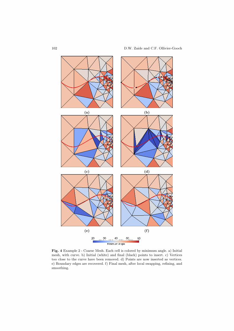
4.2 Example 2 – Graded Mesh, Cubic Spline

With the algorithm demonstrating good performance on uniform meshes, agraded mesh is examined. The initial mesh in this example has 49 vertices,with the majority of them clustered around the right boundary edge. Thecurve we wish to insert is that of section 4.1, a cubic spline. In Figure 4b, theinitial and final spacing is shown. As the mesh is graded, the initial placementof points on the curve is not as close to optimal as on the uniform mesh,and more movement and iterations of the moving mesh equation are neededbefore an optimal spacing is achieved. As in Example 1, after smoothing, norefinement is needed.

Of possible concern is the poor resolution of the curve in the final mesh(Figure 4f) due to the length scale being independent of the curve itself.This could be easily corrected in either the length scale definition or in therefinement process but we leave this for future investigation. As in the otherexamples, as the original mesh is refined, the locality of the algorithm is moreevident, with less than one percent of the original mesh modified to insertthe curve.

4.3 Example 3 – Uniform Mesh, Maple Leaf

In this example, we demonstrate the method on inserting a maple leaf shapeinto a uniform mesh. The maple leaf is defined by thirty-three lines of varyinglength, constraining the length scale based on the end points of the shortestlines. In Figure 5, the initial coarse mesh and final mesh containing the shapeare shown. Unlike the previous examples, after smoothing, some additionalrefinement is needed, with 11, 7, and 3 vertices inserted through refinementon the coarse, medium and fine initial meshes respectively. The additionalrefinement is needed around small angles, where the cell quality from theinitial vertex placement is often bad due to the angles in the maple leaf.


Comparing the initial and final meshes, Figures 5a and 5b, reveals that 78%of the initial mesh remains unchanged by the algorithm.

4.4 Example 4 – Bad Meshes, Cubic Spline

In the three examples shown, the initial mesh is of good quality. As a finaltest of the algorithm, poor quality uniform and graded meshes are generatedand used as initial meshes for the cubic spline. These meshes are generatedby randomly perturbing the good quality mesh. In Figures 6a and 6c, poorquality meshes generated from the meshes shown in Figures 3a and 4a. Thecubic spline is inserted into the mesh, and final meshes are shown in Figures6b and 6d after local smoothing and refinement. In both examples, the meshquality is improved in the near curve region, with the remainder of the meshunmodified. While the mesh is still of overall poor quality, this could be im-proved using the refinement and smoothing techniques over the whole mesh,as opposed to simply in the vicinity of the curve.

4.5 Summary

Results for each test example are summarized in Table 1. Additional re-sults for medium and fine grid examples (not pictured) are also included.Comparing minimum angles before and after the process demonstrates ouralgorithm’s effectiveness in preserving mesh quality. For each mesh, the finalquality is above 25.65◦, the minimum angle guarantee provided by the refine-ment scheme [15]. In the third example, the mesh quality decreases slightly

Table 1 Summary of Results for Examples 1-4 on meshes of increasing size. Inthis table, “Remove” is the number of vertices in cleared out to make room for,“Insert”, the number of vertices inserted on the curve. “Smooth” is to the numberof vertices moved in the smoothing process. “Min ∠” is the minimum angle of anycell in the mesh, a measure of mesh quality. Lastly, “Unch. Verts” is the numberof vertices left unchanged from the original mesh, a measure of the locality of thealgorithm.

Initial Mesh Curve Recon. # Verts Final Mesh

Example Verts Min ∠ Remove Insert Smooth Verts Min ∠ Unch. Verts

1 - Coarse 104 34.02◦ 7 11 2 108 33.31◦ 951 - Medium 8315 30.24◦ 71 112 42 8356 30.01◦ 82021 - Fine 40315 30.24◦ 157 253 110 40411 30.04◦ 40048




(a) (b)

(c) (d)

(e) (f)

Fig. 3 Example 1 - Coarse Mesh. Each cell is colored by minimum angle. a) Initialmesh, with curve. b) Initial (white) and final (black) points to insert. c) Verticestoo close to the curve have been removed. d) Points are now inserted as vertices.e) Boundary edges are recovered. f) Final mesh, after local swapping, refining, andsmoothing.


(a) (b)

(c) (d)

(e) (f)

Fig. 4 Example 2 - Coarse Mesh. Each cell is colored by minimum angle. a) Initialmesh, with curve. b) Initial (white) and final (black) points to insert. c) Verticestoo close to the curve have been removed. d) Points are now inserted as vertices.e) Boundary edges are recovered. f) Final mesh, after local swapping, refining, andsmoothing.


(a) Initial Mesh

(b) Final Mesh

Fig. 5 Example 3 - Maple Leaf - Coarse Mesh. Each cell is colored by minimumangle. a) Initial mesh, with curve. b) Final mesh, after local swapping, refining, andsmoothing. The mesh inside the maple leaf has been left unchanged, outside of alayer of vertices around the curve. The mesh inside the stem is also minimal, witha single layer of cells between bounding lines.


(a) (b)

(c) (d)

Fig. 6 Example - 4. Two initially poor quality meshes are shown on the left withthe canonical cubic spline. Final meshes are shown on the right for the two initialmeshes respectively. In both cases, the near curve region shows triangles of goodquality, while away from the curve the algorithm leaves the mesh unmodified.

due to the new complex internal geometry, but a reasonable quality is stillobtained. It important to observe that as the initial mesh size increases, asmaller percentage of the mesh is modified to insert the curve.

As a comparison for the first three examples, meshes generated from ini-tial geometry including the curve are illustrated in Figure 7. For each pair ofmeshes, there are approximately the same number of vertices. Though gen-erated in different ways, both meshes are similar in topology and quality.In Figure 7f, a mesh generated with the maple leaf as an internal boundaryhas aditional vertices placed near smaller boundary angles, a result of the


(a) Ex. 1, initial mesh gener-ated, then curve inserted

(b) Ex. 1, mesh initially gener-ated with internal boundary

(c) Ex. 2, initial mesh gener-ated, then curve inserted.

(d) Ex. 2, mesh initially gener-ated with internal boundary.

(e) Ex. 3, initial mesh gener-ated, then curve inserted.

(f) Ex. 3, mesh initially gener-ated with internal boundary.

Fig. 7 Comparison between meshes produced by curve insertion into existing mesh(left) and by generation of mesh with the curve as an internal boundary in the initialboundary geometry (right). Comparable meshes for Example 1 (top), Example 2(middle), and Example 3 (bottom).


initial Delaunay triangulation. For larger meshes, curve insertion is prefer-able and computationally less expensive than generating a new mesh. Again,the true value of our presented algorithm is in the simulation side, where min-imal mesh adjustment allows for less interpolated of simulation data, such ascell-averaged data, onto the new mesh.

5 Conclusions

In this paper we have developed and implemented an algorithm for curve in-sertion into an existing mesh. This algorithm adopts the principle of equidis-tribution from the moving mesh community to determine the location of newvertices on the curve. This results in minimal additional work in the additionof these vertices to the mesh. With the new vertices inserted, existing meshrefinement and smoothing techniques are used to produce a final mesh withthe curve as an internal boundary and acceptable mesh quality.

In three dimensions, the natural extension of the problem is inserting a sur-face into an existing tetrahedral mesh. The algorithm remains similar, with alength scale based surface mesh generated and the initial mesh cleaned up andreconnected around it, followed by smoothing and refinement. Mesh move-ment based on equidistribution for triangular meshes on a surface has beendemonstrated effectively [17, 18] and is similar to two-dimensional metric-based mesh adaptation [19]. In our algorithm, the metric would be based onthe length scale of the underlying initial mesh.

Acknowledgements. Both authors would like to acknowledge Peter Fleischmann,

Stephen Cea, Patrick Keys, and Anil Sehgal of Intel Corporation for their support.

References

1. Weatherill, N.P., Thompson, J.F., Soni, B.K. (eds.): Handbook of Grid Gener-ation. CRC Press (1999)

2. Cheng, S.W., Dey, T.K., Shewchuk, J.R.: Delaunay Mesh Generation. Chapman& Hall (2012)

3. Boivin, C., Ollivier-Gooch, C.F.: Guaranteed-quality triangular mesh genera-tion for domains with curved boundaries 55(10), 1185–1213 (2002)

4. Li, X., Shephard, M., Beall, M.: Accounting for curved domains in mesh adap-tation 58, 246–276 (2003)

5. Gosselin, S.: Delaunay Refinement Mesh Generation of Curve-bounded Do-mains. Ph. D. thesis (2009)

6. Trepanier, J.-Y., Paraschivoiu, M., Reggio, M., Camarero, R.: A conserva-tive shock fitting method on unstructured grids. Journal of ComputationalPhysics 126(2), 421–433 (1996)

7. Paciorri, R., Bonfiglioli, A.: A shock-fitting technique for 2d unstructured grids.Computers & Fluids 38(3), 715–726 (2009)


8. Huang, W., Ren, Y., Russell, R.D.: Moving mesh partial differential equations(mmpdes) based on the equidistribution principle. SIAM Journal on NumericalAnalysis 31(3), 709–730 (1994)

9. Zegeling, P.: Moving grid techniques. In: Handbook of Grid Generation, pp.37-1–37-18 (1999)

10. Stockie, J.M., Mackenzie, J.A., Russell, R.D.: A moving mesh method for one-dimensional hyperbolic conservation laws. SIAM Journal on Scientific Comput-ing 22(5), 1791–1813 (2001)

11. Cao, W., Huang, W., Russell, R.D.: A moving mesh method based on thegeometric conservation law. SIAM Journal on Scientific Computing 24(1), 118–142 (2002)

12. Shewchuk, J.R.: Delaunay Refinement Mesh Generation. Ph. D. thesis, Schoolof Computer Science, Carnegie Mellon University (May 1997)

13. Ollivier-Gooch, C.: Grummp version 0.5.0 user’s guide. Tech. rep., Departmentof Mechanical Engineering, The University of British Columbia (2010)

14. Ong, B., Russell, R., Ruuth, S.: An h-r moving mesh method for one-dimensional time-dependent PDEs. In: Jiao, X., Weill, J.-C. (eds.) Proceedingsof the 21st International Meshing Roundtable, vol. 123, pp. 39–54. Springer,Heidelberg (2013)

15. Ollivier-Gooch, C.F., Boivin, C.: Guaranteed-quality simplicial mesh genera-tion with cell size and grading control 17(3), 269–286 (2001)

16. Freitag, L.A., Ollivier-Gooch, C.F.: Tetrahedral mesh improvement using swap-ping and smoothing 40(21), 3979–4002 (1997)

17. Cao, W., Huang, W., Russell, R.D.: Anr-adaptive finite element method basedupon moving mesh PDEs. Journal of Computational Physics 149(2), 221–244(1999)

18. Crestel, B.: Moving meshes on general surfaces. Master’s thesis, Simon FraserUniversity (2011)

19. Pagnutti, D.: Anisotropic adaptation: Metrics and meshes. Master’s thesis(2008)

Documents

Inserting a Curve into an Existing Two Dimensional ...imr.sandia.gov/papers/imr22/IMR22_6_Zaide.pdf · Inserting a Curve into an Existing Two Dimensional Unstructured Mesh DanielW.ZaideandCarlF.Ollivier-Gooch