Inputandoutputinventories - Economics | Johns Hopkins …thedi!erenceisthatproductionis supplyinthedownstreammarketandusageisdemandintheupstreammarket. The"rstcolumnofFig.1showsthat"rmsdonotsynchronizedeliveriesand

�We are especially grateful to Je! Fuhrer for comments, advice, and technical assistance. Wethank the editor, Mark Bils, and an anonymous referee for particularly helpful comments, as well asLaurence Ball, Jeremy Berkowitz, David Bivin, Robert Chirinko, Simon Gilchrist, Spencer Krane,Andy Levin, Patricia Mosser, Adrian Pagan, Valerie Ramey, Robert Rossana, Ken West, JohnWilliams, and participants at numerous seminars. Brian Doyle, Catherine Humblet, andKevin Dalyprovided excellent research assistance; Hoyt Bleakley also provided valuable technical assistance.An unpublished appendix is available upon request containing derivations of the Euler equations,a detailed data description, and a discussion of the econometric procedures. Maccini thanks theNational Science Foundation for "nancial support. The opinions expressed in this paper are those ofthe authors and do not necessarily re#ect the opinions of the Federal Reserve Bank of Boston or theBoard of Governors of the Federal Reserve System.

*Corresponding author. Tel.: #1-617-973-3941; fax: #1-617-619-7541.E-mail address: [email protected] (S. Schuh).

Journal of Monetary Economics 47 (2001) 347}375

Input and output inventories�

Brad R. Humphreys�, Louis J. Maccini�, Scott Schuh��*�Department of Economics, University of Maryland Baltimore County, 1000 Hilltop Circle,

Baltimore, MD 21250, USA�Department of Economics, Johns Hopkins University, 34th & Charles Streets, Baltimore,

MD 21218, USA�Research Department, Federal Reserve Bank of Boston, P.O. Box 2076, Boston, MA 02106-2076, USA

Received 23 November 1998; received in revised form 9 May 2000; accepted 5 June 2000

Abstract

This paper presents a new stage-of-fabrication inventory model with delivery,usage, and stocks of input materials that distinguishes between gross productionand value added. It extends the linear-quadratic model of output inventories byadding the joint determination of input inventories. Empirically, input inventoriesare more important than output inventories. Maximum likelihood estimation ofthe decision rules yields correctly signed and signi"cant parameter estimates usingdata for nondurable and durable goods industries, but the overidentifying restrictions ofthe model are rejected. The value added speci"cation dominates because adjustment

0304-3932/01/$ - see front matter � 2001 Elsevier Science B.V. All rights reserved.PII: S 0 3 0 4 - 3 9 3 2 ( 0 1 ) 0 0 0 4 6 - 0

�Various authors working with aggregate data have modi"ed the basic model. Blanchard (1983),West (1986), Kahn (1992) and Fuhrer et al. (1995) add a stockout avoidance motive; Maccini andRossana (1984), Blinder (1986), Miron and Zeldes (1988), and Durlauf and Maccini (1995) add costshocks in the form of real input prices; Eichenbaum (1989) and Kollintzas (1995) add unobservabletechnology shocks; Bils and Kahn (2000) allow for the e!ects of procyclical factor utilization onmarginal cost; Ramey (1991) adds nonconvexities in production; and West (1988) adds backlogs ofun"lled orders. A consensus explanation, however, is still lacking.

costs on materials usage are critical to "tting the data. � 2001 Elsevier Science B.V.All rights reserved.

JEL classixcation: E22; E23

Keywords: Inventories; Stage-of-fabrication; Gross production; Value added

1. Introduction

Most "rms produce goods in stages. A typical "rm orders input materialsfrom an upstream supplier, takes delivery, and combines them with other factorinputs to produce "nished goods. Often during the production process the "rmgenerates its own intermediate product as well. Many "rms sell their "nishedgoods to downstream "rms, which view the goods as input materials. Thesestage-of-fabrication linkages*within and between "rms*imply that rational,optimizing "rms will be characterized by joint interaction among all aspects ofproduction. Yet macroeconomic studies of "rm behavior generally ignore suchdynamic linkages, considering materials only to measure productivity. Thispaper begins to redress this oversight.Nowhere is the neglect of stage-of-fabrication linkages more evident than in

the inventory literature, where the vast bulk of work has focused almostexclusively on "nished goods, or output, inventories. The literature, as sum-marized by Blinder and Maccini (1991), has been devoted primarily to under-standing why the rational expectations version of the pure productionsmoothing model of output inventories seems to be inconsistent with the data innondurable goods industries.� Such intense scrutiny of output inventory invest-ment has `crowded outa consideration of stage-of-fabrication linkages, such asthe ordering and usage of input materials. As a consequence, input invento-ries*de"ned here as raw materials and work-in-process*have been neglectedalmost entirely.This neglect is problematic for two reasons. First, input inventories concep-

tually are the linchpin of the stage-of-fabrication production process. They arisewhenever the delivery and usage of input materials di!er, and "rms generally donot synchronize deliveries and usage. Furthermore, since the usage of input

348 B.R. Humphreys et al. / Journal of Monetary Economics 47 (2001) 347}375

� In addition, Durlauf and Maccini (1995) "nd that real materials prices in#uence "nished goodsinventory investment, which suggests possible interaction between materials inventories and "nish-ed goods inventories.

�Related literature includes Husted and Kollintzas (1987), who o!er a rational expectationsmodel of the purchase and holding of imported raw materials inventories but ignore interaction withwork-in-process or "nished goods inventories, and West (1988), who introduces order backlogs andwork-in-process inventories into the standard output inventory model. See also the unpublishedwork of Mosser (1989) and Barth and Ramey (1997). Other work explaining interaction amonginventory types includes Lovell (1961), Feldstein and Auerbach (1976), Maccini and Rossana (1984),Reagan and Sheehan (1985), Blinder (1986), Rossana (1990), and Bivin (1993), which rely on stockadjustment and reduced-form models.

�To some degree, of course, intermediate goods*and thus work-in-process inventories*areproduced within the "rm. Hence, an important extension of this paper is to model production ofboth intermediate and "nished goods, which will require the "rm to hold separate stocks of materialsand work-in-process inventories. Extending the model to incorporate delivery lags and orderbacklogs may further improve the model's ability to "t the data.

�See Baily (1986) and Basu (1996) for discussions of the speci"cation of materials in productionfunctions and its role in explaining productivity movements.

materials is a factor of production, decisions about smoothing production andoutput inventory investment inherently are related to decisions about inputinventory investment. Second, input inventories are more important than out-put inventories empirically. Stylized facts indicate that input inventories aretwice as large and three times more variable. Moreover, the dominance of inputinventories occurs primarily in durable goods industries, which typically havebeen excluded from applied inventory research.�Despite their conceptual importance and empirical dominance, the literature

on input inventories is remarkably thin. Only Ramey (1989) has developed anoptimizing model of inventories at di!erent stages of fabrication. She, however,treats stocks of materials, work-in-process and "nished goods inventories asfactors of production and applies factor demand theory to derive demandfunctions for di!erent types of inventories. This approach does not deal ad-equately with the stock-#ow aspects of inventory holding behavior. It ignoresthe distinctions among the #ow decision to order and take delivery of materialspurchases, the #ow usage of materials in the production process, and the bene"tsand costs to the holding of stocks of input inventories. Capturing the stock-#owaspects of input inventory decisions is integral to understanding the dynamics ofmovements in such inventories.�This paper presents a new stage-of-fabrication inventory model with separate

decisions to order, use, and stock input materials. As a "rst step, we assume thatmaterials and intermediate goods are inputs purchased from outside the "rm,and that there are no input delivery lags or output order backlogs.� The modelthenmakes several advances. First, and most prominently, only the yow usage ofinput materials enters the production function, as in the productivity literature.�

B.R. Humphreys et al. / Journal of Monetary Economics 47 (2001) 347}375 349

Second, including the #ow of materials admits alternative assumptions aboutthe separability of materials in production: gross production (nonseparable) andvalue added (separable). Third, the "rm simultaneously chooses output andinput inventory investment, thus linking them with extensive cross-equationrestrictions.The model is fully structural with intertemporal cost minimization under

rational expectations and is based on several quadratic approximations likethose in conventional output inventory models. We estimate the model viamaximum likelihood, conducting the "rst joint estimation of input and outputinventory decision rules. Exploiting model identities, we overcome the lack ofhigh-frequency data on deliveries and usage of materials and estimate grossproduction and value added versions of the model with data for nondurable anddurable goods industries.On balance, the data yield reasonable econometric support for the value

added production model. All parameter estimates of the value added model arethe correct sign and estimated very signi"cantly*a degree of success quiteuncommon for applied inventory models. In contrast, the model with grossproduction yields many insigni"cant and/or implausible parameter estimates.The relative success of the value added model appears to be attributable to thepresence of adjustment costs on materials usage, which the standard grossproduction model omits. On the other hand, the data do reject the stage-of-fabrication model's overidentifying restrictions, like the vast majority of struc-tural inventory models applied to aggregate data.Several other important conclusions emerge. First, the results indicate that

aggregate cost functions are convex so that marginal cost curves slope upward,even in durable goods industries. Second, the results are consistent with theoret-ical predictions regarding both real wages and real materials costs. Third, themodel "ts the data for the durable goods industry surprisingly well despite notincluding intermediate production. Di!erences between results for nondurableand durable goods industries seem sensible. Overall, the data reveal clearevidence of stage-of-fabrication interactions between inventory stocks, andamong inventory stocks and other facets of production.The paper proceeds as follows. Section 2 updates and expands the stylized facts

about inventory movements at di!erent stages of fabrication. Section 3 presentsthe new stage-of-fabrication inventory model. Section 4 describes the econometricspeci"cation and estimation, and Section 5 reports the econometric results. Thepaper concludes with a discussion of some implications for future research.

2. Motivation and stylized facts

This section presents key empirical facts about manufacturing productionand inventory activity that motivate the stage-of-fabricationmodel developed in


�See Feldstein and Auerbach (1976), Ramey (1989), and Blinder and Maccini (1991) for priorstudies that report basic facts. We extend these studies by comparing the facts for durable andnondurable industries, by reporting facts on deliveries as well as the usage of materials, and byupdating the sample periods.

the next section.� To construct the facts, we mainly use monthly data for salesand inventories by stage of fabrication, which are in constant 1987 dollars,seasonally adjusted, and cover the period 1959:1 through 1994:5, except fordeliveries and usage of materials for which there are no data at high frequencies.We also use annual data from the Bartelsman}Gray NBER ProductivityDatabase, which includes data on usage and deliveries and covers the period1959}1994. See the data appendix for details.

2.1. Delivery and usage of input materials

Oneway to motivate the study of input inventories is to compare and contrastthe usage and deliveries of input materials with production and sales of "nishedgoods. Fig. 1 provides evidence from annual data*the only frequency availablefor deliveries and usage*on these variables in nondurable goods and durablegoods industries. Note that the di!erence between production and sales equalsoutput inventory investment, and the di!erence between deliveries and usageequals input inventory investment.Virtually all prior inventory research focuses on the extent to which "rms

synchronize production and sales. Traditional output inventory models di!er intheir predictions about the variance of production versus sales, the central issuebeing whether "rms should smooth production relative to sales. The secondcolumn of Fig. 1 shows that "rms tend to synchronize production and sales quiteclosely (correlations of 0.96 in nondurables and 1.00 in durables; ratios of produc-tion variance to sales variance of 1.02 for nondurables and 0.99 for durables).An analogous, but frequently overlooked, issue is the extent to which "rms

synchronize the deliveries and usage of materials. Usage is the upstream ana-logue of production because usage and production are very highly*though notperfectly*correlated (compare the solid lines in Fig. 1). Likewise, deliveries arethe upstream analogue of sales. Conceptually, the di!erence is that production issupply in the downstream market and usage is demand in the upstream market.The "rst column of Fig. 1 shows that "rms do not synchronize deliveries andusage nearly as closely as they do production and sales (correlations of 0.52 innondurables and 0.79 in durables; ratios of usage variance to deliveries varianceof 0.40 for nondurables and 0.53 for durables). The lack of synchronization ofdeliveries and usage is computed with annual data but it is unlikely to bereversed with higher frequency data.The relatively weak synchronization of materials delivery and usage and the

relatively strong synchronization of production and sales together imply that


Fig. 1. Annual manufacturing production activity.

input inventory investment #uctuates considerable more over time than doesoutput inventory investment. The next subsection con"rms this implicationdirectly from inventory data. However, without a structural model to interpretthe data, such as the one advanced in this paper, it is impossible to infer anythingabout "rms' cost functions or technologies that might explain the relativevariability of input inventories.

2.2. Inventory investment

A second way to motivate the study of input inventories is to compareand contrast the behavior of various components of inventory investment.Table 1 reports the means and variances of inventory investment and inventory-to-sales ratios usingmonthly data on input and output inventories in nondurablegoods and durable goods industries in U.S. manufacturing.Fact�1: Input inventories are larger and more volatile than output inventories in

manufacturing.As Table 1 indicates, input inventories are at least twice as large as output

inventories in manufacturing, as measured by average inventory investment and


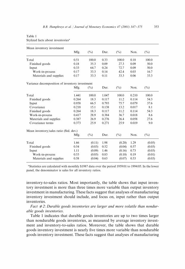
Table 1Stylized facts about inventories�

Mean inventory investmentMfg. (%) Dur. (%) Non. (%)

Total 0.51 100.0 0.33 100.0 0.18 100.0Finished goods 0.18 35.3 0.09 27.3 0.09 50.0Input 0.33 64.7 0.24 72.7 0.09 50.0Work-in-process 0.17 33.3 0.14 42.4 0.03 16.7Materials and supplies 0.17 33.3 0.11 33.3 0.06 33.3

Variance decomposition of inventory investmentMfg. (%) Dur. (%) Non. (%)

Total 1.441 100.0 1.047 100.0 0.210 100.0Finished goods 0.264 18.3 0.117 11.2 0.114 54.3Input 0.958 66.5 0.793 75.7 0.079 37.6Covariance 0.218 15.1 0.138 13.2 0.017 8.1Finished goods 0.264 18.3 0.117 11.2 0.114 54.3Work-in-process 0.417 28.9 0.384 36.7 0.018 8.6Materials and supplies 0.387 26.9 0.276 26.4 0.058 27.6Covariance terms 0.373 25.9 0.271 25.9 0.019 9.0

Mean inventory/sales ratio (Std. dev.)Mfg. (%) Dur. (%) Non. (%)

Total 1.66 (0.11) 1.98 (0.20) 1.29 (0.05)Finished goods 0.54 (0.03) 0.52 (0.04) 0.57 (0.03)Input 1.11 (0.09) 1.46 (0.16) 0.73 (0.03)Work-in-process 0.53 (0.05) 0.83 (0.10) 0.19 (0.01)Materials and supplies 0.58 (0.04) 0.63 (0.07) 0.53 (0.03)

�Statistics are calculated with monthly $1987 data over the period 1959:01 to 1994:05. In the lowerpanel, the denominator is sales for all inventory ratios.

inventory-to-sales ratios. Most importantly, the table shows that input inven-tory investment is more than three times more variable than output inventoryinvestment in manufacturing. These facts suggest that analyses of manufacturinginventory investment should include, and focus on, input rather than outputinventories.Fact �2: Durable goods inventories are larger and more volatile than nondur-

able goods inventories.Table 1 indicates that durable goods inventories are up to two times larger

than nondurable goods inventories, as measured by average inventory invest-ment and inventory-to-sales ratios. Moreover, the table shows that durablegoods inventory investment is nearly "ve times more variable than nondurablegoods inventory investment. These facts suggest that analyses of manufacturing


inventory investment should include, and focus on, durable rather than nondur-able goods inventories.Fact �3: Input inventories are much larger and more volatile than output

inventories in durable goods industries, but input and output inventories are similarin size and volatility in nondurable goods industries.

This fact is a byproduct of the "rst two. Table 1 indicates that input inventoriesare much larger than output inventories in durable goods industries, as measuredby average inventory investment and inventory-to-sales ratios. Further, the tableshows that input inventory investment is more than six times more variable thanoutput inventory investment in durable goods industries. In nondurable goodsindustries, on the other hand, the magnitude and variability of input inventoriesare more even with those of output inventories. In nondurables, input inventoryinvestment is a bit larger but a bit less variable than output inventory investment.The fact that output inventory investment is a bit more variable than inputinventory investment provides some rationale for the literature's focus on outputinventory investment in nondurable goods industries. Nevertheless, it is di$cultto rationalize the nearly complete focus on output inventories in nondurables;instead, the focus should be on input inventories in durables.Fact �4: Interactions between input and output inventories are quantitatively

signixcant, especially in durable goods industries.The middle panel of Table 1 quanti"es the extent of inventory stock interac-

tion. Fifteen percent of the variance in manufacturing inventory investment isaccounted for by the covariance between input and output inventory invest-ment. When the inventory stocks are disaggregated into the three stages ofprocessing (materials, work-in-process, and "nished goods), the covarianceterms account for 26 percent of the variance. The table also shows thatcovariance among types of inventory investment is greater in durable goodsindustries than nondurable goods industries (26 percent versus 9 percent).Together, these four stylized facts suggest the following main conclusions:

(1) a complete analysis of total manufacturing inventory behavior requires themodeling of input inventories; (2) tests of inventory models should be conductedwith durable goods, as well as nondurable goods, industries; and (3) interactionbetween input and output inventories is empirically evident and potentiallya signi"cant feature of "rm behavior.

3. The stage-of-fabrication model

3.1. Overview

Fig. 2 provides a schematic illustration of the model, which focuses on #owsthrough the stage-of-fabrication production process employed by a "rm to


Fig. 2. Stage-of-fabrication model diagram.

�Actually, the "rm chooses ¸, ;, and D, but because there are no high-frequency data availableon ; and D we use the model #ow identities and "rst-order conditions to recast the problem withinventory stocks as choice variables.

transform input inventories (raw materials and work-in-process) into outputinventories ("nished goods). Each period, the "rm combines labor (¸), materialsused in production (;), and capital (K) to produce "nished goods. Materialsused in production are obtained from the on-hand stock of input inventories(M), which is continually replenished by deliveries (D) of materials from foreignand domestic suppliers. Production (>) of "nal goods is added to the stock ofoutput inventories (N), which are used to meet "nal demand (X). The "rm takes"nal demand, the price of labor (=), and the price of material deliveries (<) asexogenous (thin lines).The "rm optimizes in a dynamic stochastic environment. In the short

run, with capital "xed, the "rm chooses ;, M, and N to minimize thepresent value of total costs, given <, =, and X, for a total of six variablesand equations in the model.� Six random shocks (�)*one for each equation inthe model*bu!et the "rm's production environment. One shock is a demandshock (�

�). The other shocks comprise a disaggregation of the traditional

`supplya shock: a technology shock (��) a!ects the production function; inven-

tory holding cost shocks (��,��) a!ect the costs of carrying inventory stocks;

a real wage shock (��) a!ects labor costs; and a real materials price shock (�

�)

a!ects material costs.The model generalizes the traditional linear-quadratic model of output inven-

tories. The central extension in the stage-of-fabrication model is the explicitintroduction of input inventories, which must be chosen simultaneously withoutput inventories. Input inventory investment is controlled by varying theusage of materials in production and the deliveries of materials. Totalcosts*labor costs, inventory holding costs, and delivery costs*are approxi-mated with a generalized quadratic form. Our stage-of-fabrication model di!ersfrom the few inventory papers that include input inventories by specifying the#ow, rather than stock, of materials in the production function. For the purpose


In future work, we intend to estimate the stage-of-fabrication model with inventory data fromthe "rm-level M3LRD data base originally developed by Schuh (1992). An advantage of workingwith individual "rm data is that the accuracy of distinguishing inventories at di!erent stages offabrication is enhanced.

To allow for production of intermediate goods within the "rm requires extending the productionfunction to incorporate joint production of "nal and intermediate goods. This extension is a sub-stantial modi"cation of the standard production process that we leave for future work.

of testing the model with aggregate data, we adopt the convention of a represen-tative "rm, as is customary in the inventory literature.

3.2. The production function

Following the literature on production functions and productivity*forexamples, see Baily (1986) and Basu (1996)*we assume that the short-runproduction function contains as an input the #ow of materials used in theproduction process. Speci"cally, the production function is

>�"F(¸

�,;

�,��). (1)

Note that ;�is the yow of materials used in the production process, not the

stock of materials inventories. Because >�is gross output, we refer to Eq. (1) as

the gross production function. Two assumptions are implicit in (1): First, thecapital stock is a "xed factor of production with no short-run variation inutilization*an unrealistic assumption that should ultimately be relaxed ina more complete model of production. As a consequence, the remaining fac-tors*materials usage and labor*possess positive and nonincreasing marginalproducts, and the short-run production function exhibits decreasing returns toscale. Second, the "rm purchases intermediate goods (work-in-process) fromoutside suppliers rather than producing them internally. Thus, intermediategoods are analogous to raw materials so work-in-process inventories can belumped together with materials inventories.An important speci"cation issue for the production function is whether ;

�is

additively separable from the other factors of production. For example, Basuand Fernald (1995) show that evidence of externalities caused by productivespillovers exists in value added data but not gross production data. If ;

�is

separable, then the production function can be written as

>�!H(;

�)"G(¸

�,��), (2)

where >�!H(;

�) is value added. For this paper, we make the strong simplify-

ing assumption thatH(;�)";

�. Consequently, Eq. (2) is a special case of Eq. (1)

with the restrictions F�

"1 and F�

"F��"0. We refer to this form of theproduction function as the value added production function.


By specifying the #ow usage of input materials in the production function, weextend traditional inventory models to include an additional role for inventorydynamics (investment) in the stage-of-fabrication process. Previous inventorymodels focus solely on the role of inventory stocks as a convenience yield to the"rm. Typically this convenience yield is interpreted as the savings of lost sales bythe "rm when it cannot satisfy customers, but it has also been interpreted as thesavings in marketing costs (see Pindyck, 1994). The few inventory models thatconsider both input and output inventories, such as Ramey (1989) and Con-sidine (1997), include inventory stocks in the production function. In this case,the bene"ts to holding inventory stocks are interpreted as bene"ts to thephysical production process itself, for example the avoidance of productiondisruptions. None of these speci"cations, however, incorporates the #ow dy-namics implied by the delivery and usage of materials for input and outputinventory investment.

3.3. The cost structure

The "rm's total cost structure consists of three major components: labor costs,inventory holding costs, and materials costs. This section describes each com-ponent.

3.3.1. Labor costsLabor costs are

¸C�"=

�¸

�#A(�¸

�) (3)

with

A��0 as �¸��0

A�'0

where �¸�"¸

�!¸

��. The "rst component,=

�¸�, is the standard wage bill.

The second component,A(�¸�), is a standard adjustment cost function intended

to capture the hiring and "ring costs associated with changes in labor inputs.The adjustment cost function has the usual properties, including a risingmarginal adjustment cost.To focus on inventory decisions, we eliminate labor input. Inverting the

production function, equation (1), yields the labor requirements function

¸�"¸(>

�,;

�,��). (4)

Substituting (4) into (3) yields

¸C�"=

�¸(>

�,;

�,��)#A(¸(>

�,;

�,��)!¸(>

��,;

��,��

)) (5)


��The restrictions are implied by the strict concavity of the short-run-production function and thestrict concavity of the adjustment cost function.

which is the central portion of the "rm's cost function. Observe that, whenmaterials usage is taken into account in the production function, the invertedproduction function implies that adjustment costs depend on the change inmaterials usage as well as the change in gross output, a feature which thestandard model overlooks.Following the inventory literature, we approximate Eq. (5) with a generalized

quadratic function. Speci"cally, labor cost is

¸C�"�

��2 �>�

�#�

��2 �;�

�#�

�>

�;

�#=

�[�

�>

�#�

�;

�]

#��

2�[��>�#�

��;

�]�#�

��(�

>

�#�

;

�) (6)

with the parametric restrictions

��,��,��'0 �

�(0 �

�,�,(�

��!��

�)*0 �

�,��,�)0

implied by the production function.��We focus on two production function speci"cations: gross production and

value added. The cost function approximation is extensively parameterized,which makes it di$cult to estimate all parameters precisely. Hence, somerestrictions must be imposed. We choose restrictions that capture the essentialfeatures of our model but yield the standard output inventory model as a specialcase.Gross production: To obtain the gross production speci"cation, let

��"�

�"�

"0, �

�"!�

"1.

Then the gross production (g) cost function is

¸C�"�

��2 �>�

�#�

��2 �;�

�#�

�>

�;

�#�

�=

�>

�#�

�

2�(�>�)�!�

��>

�.

(7)

The standard output inventory model cost function is a special case of Eq. (7)and can be obtained by setting �

�"�

�"0, an assumption implicit in the

standard model. The restriction ��"0 usually is imposed as well, with Eichen-

baum (1984) and Durlauf and Maccini (1995) being exceptions. This speci"ca-tion directly extends the standard model by allowing for materials usage in theproduction process, but not in adjustment costs.


Value added: To obtain the value added speci"cation, let

��"�

�"!�

�"�'0, �

�"!�

�'0,

��"!�

�"!�

"�

"1.

These restrictions make value added, >�!;

�, a factor in the inverted produc-

tion function, rather than >�and ;

�separately. Then the value added (v) cost

function is

¸C��"�

�2�(>�

!;�)�#�

�=

�(>

�!;

�)

#��

2�(�>�!�;

�)�!�

��(>

�!;

�). (8)

The standard output inventory model is also a special case of Eq. (8), and can beobtained by setting ;

�"0 for all t.

Comparing Eqs. (7) and (8) emphasizes that introducing materials usagemakes the cost function critically dependent on the speci"cation of the techno-logy. The value added speci"cation has several advantages. One is that it isconsistent with the prevailing treatment of production technology. Another isthat it is more parsimonious and thus potentially easier to estimate.Finally, and most importantly, the value added speci"cation highlights a very

restrictive and previously unrecognized assumption implicit in standard outputinventory models. The value added speci"cation inherently imposes adjustmentcosts on the change in value added, which implies that adjustment costs dependon the change in materials usage (�;

�) as well as on the change in gross output

(�>�). As we show later, the appearance of the change in materials usage in

adjustment costs has important implications for the model's dynamic structure,especially for the persistence of input inventories.

3.3.2. Inventory holding costsIn line with much of the output inventory literature, holding costs for output

inventories are a quadratic approximation to actual costs of the form

HC��"(�

�#�

��)N

�#�

�2�(N�

!NH�)�, (9)

where ��is the white noise innovation to output inventory holding costs, NH

�is

the target level of output inventories that minimizes output inventory holdingcosts, and �'0. We adopt an analogous formulation for input inventories;holding costs for these stocks are a quadratic approximation of the form

HC��

"(��#�

��)M

�#�

�2�(M�

!MH�)�, (10)


where ��is the white noise innovation to input inventory holding costs, MH

�is

the target level of input inventories that minimizes input inventory holdingcosts, and �'0. The quadratic inventory holding cost structure balances twoforces. Holding costs rise with the level of inventories, M

�and N

�, due to

increased storage costs, insurance costs, etc. But holding costs fall with M�and

N�because*given expected MH

�and NH

�*higher M

�and N

�reduce the likeli-

hood that the "rm will `stock outa of inventories.Finally, it remains to specify the inventory target stocks. Again following the

literature, the output inventory target stock is

NH�"�X

�, (11)

where �'0. The output inventory target depends on sales because the "rmincurs costs due to lost sales when it stocks out of output inventories. For theinput inventory target stock, we assume that the target stock depends onproduction, rather than sales. In particular,

MH�">

�, (12)

where '0. The input inventory target depends on production(>

�"X

�#�N

�) because stocking out of input inventories also entails costs

associated with production disruptions*lost production, so to speak*that aredistinct from the cost of lost sales. Lost production may be manifested byreduced productivity or failure to realize production plans.To summarize, the input and output inventory targets di!er because the "rm

holds the two inventory stocks for di!erent reasons. The "rm stocks outputinventories to guard against random demand #uctuations, but it stocks inputinventories to guard against random #uctuations in productivity, materialsprices and deliveries, and other aspects of production. Although sales andproduction are highly positively correlated, they di!er enough at high frequen-cies to justify di!erent target stock speci"cations.

3.3.3. Input materials costsInput materials costs consist of purchase and adjustment costs. Speci"cally,

input materials costs are

MC�"<

�D

�#�

�

2�D��. (13)

The "rst term on the right side of Eq. (13) is the cost of ordering andpurchasing input materials at the `basea price each period. This term is the onlyone in the model without a parameter, and it permits identi"cation of allremaining parameters (except target stock parameters, which are identi"ed


��See West (1993) for a discussion of identi"cation in inventory models.

��This is analogous to the literature on adjustment cost models for investment in plant andequipment where external adjustment costs are imposed in the form of a rising supply price forcapital goods.

separately) relative to the units in which <�is measured.�� The second term is

a quadratic approximation for adjustment costs on purchases of materials andsupplies.On adjustment costs, two cases may be distinguished:

1. Increasing marginal cost: �'0. In this case, the "rm faces a rising supplyprice for materials purchases. The "rm thus experiences increasing marginalcosts to purchasing materials due to higher premia that must be paid toacquire materials more quickly. A rationale for such a rising supply price isthat the "rm is a monopsonist in the market for materials. This is most likelyto occur when materials are highly "rm or industry speci"c and the "rm orindustry is a relatively large fraction of market demand.�� The rising mar-ginal cost of course gives rise to the `smoothinga of purchases.

2. Constant marginal cost: �"0. In this case, "rms are price takers in competi-tive input markets and purchase all the rawmaterials needed at the prevailingmarket price.

3.4. Cost minimization

To focus on the cost minimization problem, we assume that inventories donot enter the "rm's revenue function, and that the materials price and wage areboth exogenous to the "rm. Thus, the "rm chooses ;

�,M

�,N

��

to minimizethe discounted present value of total costs (TC),

E�

��

��(¸C�#HC�

�#HC�

�#MC

�), (14)

where �"(1#r)�� is the discount factor implied by the constant real rate ofinterest r. The two laws of motion governing inventory stocks,

�N�">

�!X

�, (15)

�M�"D

�!;

�, (16)

can be used to substitute for production (>�) and deliveries (D

�).

3.5. Euler equations

The model yields Euler equations for;�,M

�, andN

�. However, because there

are no high-frequency data on usage, ;�must be eliminated from the Euler


��See the unpublished appendix for the details of the derivation.

equations for empirical work to proceed. We thus use the Euler equation formaterials usage to eliminate;

�from the system. After some straightforward but

tedious algebra, collecting terms around common parameters, and imposing therelevant restrictions, the Euler equations for each production speci"cation canbe derived.��To present the Euler equations in a concise fashion, de"ne the lag operator as

¸, which works as a lead operator when inverted (e.g., ¸��>�">

� �), and

a variable Z��that denotes quasi-di!erences (1!�¸��) of model vari-

ables. Subscript i indicates the variable being quasi-di!erenced, subscript jindicates the number of quasi-di!erences, (1!�¸��)�, and �"(1!¸) is thestandard "rst-di!erence operator. Three examples clarify the notation:Z

��"(1!�¸��)>

�is the quasi-"rst di!erence of >

�; Z

��"(1!�¸��)�>

�is

the quasi-second di!erence of >�, and �Z

��"(1!¸)(1!�¸��)�>

�"

(1!�¸��)��>�is the change in the quasi-second di!erence. Similar notation

applies for all other variables except the inventory target terms.Using this notational convention, the Euler equations for the two production

speci"cations can be presented as follows:Gross production model: The Euler equation for input inventories is

E��

��Z��

#��Z

��!�

��Z

��#�(�

�#�)[M

�!>

�]

#(��#�)Z��"0 (17)

and the Euler equation for output inventories is

E�(�

�! �

�)Z

��#�Z

��#�[N

�!�X

�]#�

�Z

��! Z

��

! �[M�!>

�!�(M

� �!>

� �)]!� Z��

#Z��#Z��"0

(18)

where "��/(�

�#�).

Value added model: The Euler equation for input inventories is

E��Z��

#��Z��#�Z

��#�Z

��#��

�Z

��#��Z

��#��Z

��

# �(�#�)(M�!>

�)#��[�M

�!�>

�!�(�M

� �!�>

� �)]

!�Z��#(��#�)Z��#��Z��#�

��"0 (19)

and the Euler equation for output inventories is

E��(�#�)(N

�!�X

�)#��(�N

�!��X

�)

! �(�#�)[(1#)(M�!>

�)!�(M

� �!>

� �)]


�� In principle, it would be informative to solve analytically for the decision rules of the completesystem. These rules would show analytically the impact of the dynamic linkages imposed by themodel on production and inventory investment. Unfortunately, however, the models are a sixth-order di!erence equation system in M and N, and such systems are very di$cult, perhapsimpossible, to solve analytically.

! ��[(1#)(�M�!�>

�)!�(�M

� �!�>

� �)]

# (�#�)Z��#�Z��!(�#�)Z��!�Z��#��"0, (20)

where �'0 is the parameter attached to the cost of producing value added.An important issue on which the inventory literature has focused is the slope

of the marginal cost of production. The traditional linear-quadratic outputinventory model assumes rising marginal cost due to diminishing returns to thevariable factors in the short-run cost function, which induces a productionsmoothing motive. The slope of marginal cost in the stage-of-fabrication model,obtained from the second derivative of the dynamic total cost function, is

��¹C/�>�"��#(1#�)� (21)

for the gross production models; the formula for value added is the same exceptthat � replaces �

�. For both models, the slope of marginal cost should be positive

from the concavity of the production function.

3.6. Interpretation of Euler equations��

The input inventory Euler equations, (17) and (19), which represent newcontributions to the literature, embody standard economic behavior for a gen-eric quadratic regulator problem. Consider "rst the gross production case. The"rm attempts to set the input inventory stock equal to its target subject toseveral dynamic frictions. First, the adjustment costs associated with purchasesand deliveries of materials, quanti"ed by �, prevent the "rm from instantaneous-ly eliminating input inventory gaps, M

�!>

�. Second, time variation in ex-

pected materials prices gives the "rm an incentive to intertemporally substitutedeliveries of input materials. Bargains on input materials must be large enoughto more than o!set adjustment and stockout costs. Finally, higher outputinventory stocks induce the "rm to raise gross production, which in turnrequires higher materials usage and thus tends to draw down materials inven-tory stocks.Consider next the input inventory Euler equation in the value added case. It

contains the same forces at work as in the gross production case, albeit with thevalue added restrictions �

�"�

�"!�

�"� imposed. The key extension of the

value added case is that, because adjustment costs depend on the change invalue added, they depend on changes in materials usage as well as changes ingross output. Hence, changes in the second di!erences of the relevant variables


that appeared in the gross production equation enter the value added equationas well. These are captured by the terms involving the slope of the marginaladjustment cost of labor, �. These forces tend to impart additional persistenceon materials stocks.The output inventory Euler equations, (18) and (20), extend the standard

output inventory model in the literature by explicitly introducing input mater-ials. The "rst line of Eq. (18), which assumes gross production, represents themost general standard model. Thus, introducing input materials expands thestandard model in two ways. First, it adds a quasi-di!erence of the inputinventory gap to the equation. Second, the adjustment costs associated withmaterials deliveries a!ect the extent to which materials can be used in producingoutput and thus the accumulation of output inventory stocks. By omitting thesevariables, the standard output inventory model implicitly imposes theoreticalrestrictions that may contribute to its poor econometric performance.In contrast, Eq. (20), which assumes value added, di!ers markedly from the

standard output inventory model. In particular, only input and output inven-tory gap terms appear in the Euler equation because the value added restrictionseliminate the nongap terms. As a result, the value added output inventory modelreduces to a relatively simple case of balancing input and output inventory gaps.Interestingly, the cost of frictions in the value added model are manifest throughchanges in the inventory gaps rather than through changes in production, as inthe standard model.Input and output inventory stocks interact directly and indirectly in the

stage-of-fabricationmodel, and the modes of interaction are essentially the samein the gross production and value added versions of the model. Input inventoriesdirectly a!ect output inventories through the input inventory gap in the outputinventory Eqs. (17) and (19). All else equal, an increase in the input inventory gapraises current and, due to adjustment costs, future output inventories.The intuition behind this result is simple. Suppose the "rm starts with zero

inventory gaps. Then an increase in the input inventory gap involves a stockoutcost. Because the stockout costs for both inventory types are quadratic, it iscost-minimizing to spread the stockout costs between inventory stocks ratherthan have one zero and one nonzero gap. The "rm spreads excess input stocksbetween input and output inventories by drawing down input inventoriesthrough increased usage (and, hence, production). Given sales, this actionnecessarily raises the output inventory gap. Obviously, the extent of stockspreading that occurs depends on the actual magnitudes of production, adjust-ment, and output inventory stockout costs relative to input inventory stockoutcosts.On the other hand, output inventories indirectly a!ect input inventories

through the input inventory target stock,MH�, in Eqs. (18) and (20). All else equal,

an increase in output inventories raises production,>�, and thusMH

�by a factor

of , thereby reducing the input inventory gap. The "rm's optimal response to


��See West and Wilcox (1994) and FMS, and references therein.

��The GMM parameter estimates are mostly insigni"cant and highly sensitive to variations innormalization, instrument set, and other asymptotically irrelevant speci"cations. See also Hump-hreys (1995) for a discussion of problems with GMM estimation of a similar inventory model.

��For details on solution and estimation, see FMS and Humphreys et al. (1997).

this change is to increase input inventories, albeit less than completely due toadjustment cost frictions. This indirect interaction is the main source of cross-equation restrictions in the model. In addition to this force, higher outputinventory stocks generate higher production of "nished goods which raisesmaterials usage and thus draws down materials inventory stocks.

4. Econometric speci5cation and estimation

Following Blanchard (1983), Eichenbaum (1984), and Fuhrer et al. (1995)(FMS), we estimate the stage-of-fabrication model by applying maximum likeli-hood to the decision rules rather than GMM to the Euler equations. Threefactors argue for the maximum likelihood approach. First, instrumental vari-ables estimators such as GMM tend to exhibit substantial biases and impreci-sion in small samples.�� Second, FMS demonstrates that maximum likelihoodestimates of a benchmark linear-quadratic output inventory model are lessbiased and more signi"cant than GMM estimates in small samples. Third, our(unreported) attempts to estimate the model with GMM produced typicaldi$culties.��Our estimation of the new stage-of-fabricationmodel is the most comprehens-

ive to date. We estimate structural parameters from decision rules for outputand input inventories jointly, imposing all cross-equation restrictions and trans-versality conditions. Furthermore, the maximum likelihood estimation permitsexamination of the dynamic properties of the inventory system.The stage-of-fabrication model is a system of "ve equations: two Euler

equations for the endogenous inventory stocks, M�and N

�, and three

autoregressive auxiliary models for the variables <�, =

�, and X

�. Following

the bulk of the output inventory literature, we treat sales as exogenous in theestimation. In future work it will be important to relax this assumption. Thesystem can be solved using the procedure developed by Anderson and Moore(1985), which generalizes Blanchard and Kahn (1980).�� We use a two-stepapproximation to full-information maximum likelihood, in which parameters ofthe auxiliary models are estimated with OLS in the "rst step. This estimator isless e$cient but asymptotically equivalent to full-information estimation andconsiderably faster*a major consideration given the complexity of the jointmodel.


�A worthwhile extension of this paper would be to estimate the models using more disaggregateddata, such as the twenty nondurable and durable goods 2-digit SIC industries. However, theestimation process is extremely di$cult and time consuming because of the extensive cross-equationrestrictions, so we leave this substantial task for future work.

�Also, time variation in the discount rate makes the model nonlinear in variables, which oursolution and estimation methodology does not allow. Ultimately, however, it would be preferable toincorporate a time-varying discount rate, as in Bils and Kahn (2000).

We estimate the gross production and value added versions of the model withaggregate data for nondurable goods and durable goods industries.� Followingthe bulk of the applied inventory literature, we use data log detrended withlinear and quadratic trends; results are qualitatively similar for data detrendedwith an HP "lter. All regressions cover the period 1959:1 to 1994:5, lessappropriate lags. The discount factor, �, is preset at 0.995, a common practicefor structural estimation of this sort.� Standard errors are calculated using themethod of Berndt et al. (1974).

5. Econometric results

This section reports econometric results for the stage-of-fabrication inventorymodels. Table 2 contains the joint maximum likelihood estimates for the grossproduction (GP) and value added (VA) models, plus a generalized gross produc-tion (GGP) model that is explained later in this section. ��¹C/�>� is theestimate of the slope of marginal cost. 2(L!LR) is the �� statistic from thelikelihood ratio test of the model's overidentifying restrictions, where LR de-notes the likelihood of the restricted stage-of-fabrication model and L is thelikelihood of the unrestricted reduced form of the stage-of-fabrication model.The p-values are in parentheses.

5.1. General results for GP and VA

The overall impression conveyed by Table 2 is that the parameter estimatesfor the VA model are consistent with the predictions of the model in bothindustry groups but those from the GP model are not. Every VA parameter isestimated signi"cantly at the 5 percent level or better, and all estimates are thecorrect sign predicted by the model. In contrast, half or fewer of the GPparameters are estimated signi"cantly, and some are the incorrect sign (�

�should be negative and �

�should be positive). Moreover, the magnitudes of the

VA parameters are much more plausible and quite di!erent than those of theGP parameters.Quantitatively, the main di!erences between the GP and VA models arise in

the target stock (�,), adjustment cost (�), and delivery cost (�) parameter


Table 2Stage-of-fabrication model estimates�

Nondurables Durables

Parameter GP VA GGP GP VA GGP

� 7.85� 0.76� 0.99� 4.84 0.77� 0.22�(1.08) (0.09) (0.21) (7.33) (0.07) (0.06)

2.42� 1.09� 1.37� 1.48 1.52� 0.84�(0.35) (0.08) (0.20) (2.08) (0.09) (0.06)

� 2.15� 1.09�(0.42) (0.16)

��

0.23 6.44 1.01� 2.67�(0.51) (6.92) (0.40) (1.57)

��

0.15 3.29 0.47� 1.16�(0.88) (3.26) (0.17) (0.55)

��

0.001 5.84� 0.02� 1.88�(0.07) (2.10) (0.01) (0.85)

��

!0.03 9.21� 4.04 0.02 34.2� !9.02�(0.05) (4.41) (3.92) (0.05) (2.90) (3.64)

� 0.002 0.79� 5.08� 0.010� 0.65� 1.70�(0.20) (0.13) (1.78) (0.004) (0.07) (0.40)

� 0.00009 0.89� 0.98� 0.0006� 0.32� 2.94�(0.001) (0.10) (0.41) (0.0001) (0.03) (0.42)

� 0.12 2.02� 8.16� 0.28 6.21� 2.64�(2.40) (0.17) (2.21) (0.19) (0.34) (0.58)

� 134.2� 1.20� 7.39� 86.9 2.08� 3.30�(1.35) (0.03) (1.78) (197.4) (0.11) (0.83)

��¹C/�>� 0.47 6.19� 22.7� 1.57� 13.5� 7.95�(0.51) (0.26) (4.54) (0.59) (0.73) (0.95)

2(L!LR) 0.00 0.00 0.00 0.00 0.00 0.00

�The models are estimated with maximum likelihood over the period 1959:1 through 1994:5, lessappropriate lags. GP denotes gross production, VA denotes value added, and GGP denotesgeneralized gross production. Asymptotic standard errors are in parentheses except for 2(L!LR),which is the p-value.�Signi"cance at the 5 percent level. See the text for details.

estimates. The VA target stock estimates are highly signi"cant and close to theaverage inventory-sales ratios reported in Table 1. Also, the estimate of � is quiteconsistent with estimates from standard output inventory models reported inthe literature. In contrast, GP estimates of � imply that "rms aim to holdinventory stock "ve to eight times larger than monthly sales, which clearly isimplausible. GP estimates of are more reasonable, but still two and one-halftimes larger in nondurables; both GP target stock parameters in durables areinsigni"cant. GP estimates of � are 40 to 100 times larger than the VA estimates,


while the GP estimates of � are about an order of magnitude smaller andinsigni"cant.These substantial di!erences in parameter estimates between the two models

illustrate the econometric consequences of failing to include materials usage inthe labor adjustment cost speci"cation of the GPmodel. To understand this, it isimportant to note that the inventory gaps, M

�!>

�and N

�!�X

�, are extra-

ordinarily persistent, so inventory stocks deviate from their targets for very longperiods*often many years.It is well recognized that this persistence requires a cost of changing gross

production in the standard output inventory model to justify sluggish inventoryadjustment and "t the data. Because they include another (persistent) inventorystock, the stage-of-fabrication models also require an additional source ofadjustment costs to "t the data. Implicitly, the GP model contains a cost ofadjusting input inventory stocks via delivery costs, (�/2)D�

�"(�/2)(;

�#�M

�)�.

But absent a cost of changing materials usage, the "rm can vary usage and valueadded quickly and costlessly.These characteristics help explain the econometric estimates. In the GP

model, absence of an extra smoothing motive for usage and value added leads tovery high estimates of delivery costs to justify persistent input inventory behav-ior. These costs are estimated to be so large that the "rm maintains enormousoutput inventory stocks to guard against demand shocks. Such shocks wouldrequire substantial changes in production, which can be accommodated easilythrough changes in usage even though changes in labor are implicitly costly. Theonly way to prevent this output adjustment is to keep deliveries from changingmuch, and this explains the very high estimates of slope of marginal deliverycosts (�). Without adjustment costs on changing materials usage, the cost ofadjusting labor is improperly speci"ed and thus its slope (�) is estimated to besmall and insigni"cant.In contrast, the VA model includes a cost of changing materials usage. Note

that, using the identity;�"D

�!�M

�, placing an adjustment cost on changing

materials usage (�;�) implicitly places a cost on adjusting the change in input

inventory investment (��M�). This imparts additional persistence on input inven-

tory stocks and alleviates the need to get persistence through higher estimates ofthe slope of marginal delivery costs. Instead, adjustment costs are spread evenlythrough the production process, and estimates of the slopes of marginal deliverycosts and marginal labor adjustment costs are more reasonable. As a practicalmatter, the VA model includes more lags and more variables, both of whichprovide supplementary channels by which to capture persistence.

5.2. Exploring a hybrid model

Table 2 also includes results for a generalized gross production (GGP)model, a hybrid of the GP and VA models designed to determine why the


��To obtain the generalized gross production speci"cation, let

��"!�

�, �

�"!�

�"!�

"�

"1.

Then the generalized gross production (gH) cost function is

¸CH

�"(��

�)>�

�#(��

�);�

�#�

�>

�;

�#�

�=

�(>

�!;

�)#(�

�)(�>

�!�;

�)�!�

��>

�. (22)

A more general speci"cation would leave ��and �

�unrestricted, but we adopt the VA model

restrictions on these parameters to isolate the e!ect of the value added restriction on the productionfunction only. The Euler equation for input and output inventories, respectively, are

E�!��

�Z

��#��Z

��#�

��Z��

#��Z��#�

�Z

��#�Z

��#��

�Z

��

#(��#�)�[M

�!>

�]#��[�M

�!�>

�]!�Z��#(�

�#�)Z��#�Z��"0 (23)

E�[�

�(�

�#�)!��

�]Z

��#�(�

�#�#2�

�#�

�)Z

��!�

��Z��

#��Z��

!��Z

��#�Z

��#�

�(�

�#�

�#�)Z

��!�(�

�#�)[M

�!>

�!�(M

� �!>

� �)]

!��[�M�!�>

�!�(�M

� �!�>

� �)]#�(�

�#�)[N

�#�X

�]

#��[�N�!��X

�]![�

�#�

�#�]Z��#�Z��#(�

�#�)Z��"0 (24)

Derivation of this model is available in the unpublished appendix.

VA model produces better estimates. Like the VA model, the GGPmodel incorporates the change in materials usage in the adjustmentcost component of the labor cost function, but it does not impose the VArestriction on production. Thus the GGP results help determine whether adjust-ment costs on the change in materials usage are responsible for the improvedestimates.��Estimation of the GGP model provides a test of this hypothesis for the

di!erence between estimates of the GP and VA model. If the hypothesis iscorrect, then the value added production speci"cation (�

�"�

�"!�

�"�)

should not be the reason the model has trouble "tting the data. Instead, theassumption that adjustment costs do not depend on the change in materialsusage (�

�"0) should be the reason.

As the table shows, the GGP model estimates are much closer to the VAmodel estimates. In particular, the GGP target stock estimates are considerablysmaller and much more plausible. Also, the estimates of � are much smaller andthe estimates of � much larger, though they are still larger and smaller,respectively, than in the VA model. GGP estimates of both of these parametersare signi"cant as well. Despite these improvements, however, the GGP estimatesare not quite as supportive of the model as the VA estimates. Several GGPestimates are still insigni"cant, plus the �

�and �

�signs are still mostly incorrect.

Thus, there appears to be additional bene"t to imposing the VA restriction onthe production process, which leads to notably di!erent structure of the Eulerequations.


��Bresnahan and Ramey (1994) report evidence of nonconvexities in auto production plantsresulting from the "xed costs.

5.3. Specixc results

Beyond the general conclusion that the VA model "ts the data better, severalmore speci"c conclusions emerge from the VA results:

Convexity*The slope of marginal cost is positive and signi"cant, indicatingthat aggregate cost functions are convex and providing additional evidenceagainst Ramey's (1991) claim to the contrary. Our results extend the evidenceagainst nonconvex aggregate costs in two ways. First, aggregate costs are evenmore convex in durable goods industries, where nonconvexities are most oftensurmised to arise, at least at the micro level.�� Second, the results point toconvex costs even in the presence of input inventories. If material costs arelinear, or there are "xed ordering costs, input inventories would follow noncon-vex (S, s) rules that presumably could spill over into production behaviorthrough stage-of-fabrication linkages.Wages and prices*The results are generally consistent with theoretical pre-

dictions regarding real wages and materials prices. Marginal labor costs, ��, are

positive and signi"cant in the VA model. Although there are no speci"c para-meters associated with real materials costs, the forward-looking speculativebehavior implied by the model receives support from the overall success of theVA model in particular. Thus, the stage-of-fabrication model di!ers from manyprevious attempts to include real wages and materials prices in inventorymodels.Industrial heterogeneity*Several di!erences arise between the results for

nondurable and durable goods industries. Marginal adjustment costs are largerfor durable goods industries. Labor adjustment costs (�) are about three timeslarger and delivery adjustment costs (�) are about twice as large. In contrast, themarginal cost of inventory stockout costs (�,�) are smaller in durable goodsindustries, and the marginal cost of input inventory stockouts (�) is smallerrelative to the marginal cost of output inventory stockouts in durables. Mar-ginal wage costs (�

�) are about three times larger in the durable goods industry.

Finally, the slope of marginal cost appears to be higher in the durable goodsindustry, at least for the VA model.Overidentifying restrictions*The only substantive shortcoming of the model

is that the overidentifying restrictions are overwhelmingly rejected. This rejec-tion is a well-known problem that plagues not only inventory models but moststructural macroeconomic models applied to aggregate data. The reason for therejection is that the model residuals are extremely persistent, as they are instandard output inventory models. Schuh (1996) and Krane and Braun (1991)


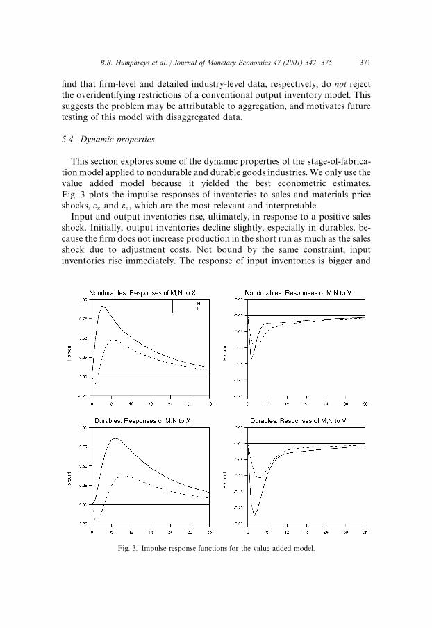
Fig. 3. Impulse response functions for the value added model.

"nd that "rm-level and detailed industry-level data, respectively, do not rejectthe overidentifying restrictions of a conventional output inventory model. Thissuggests the problem may be attributable to aggregation, and motivates futuretesting of this model with disaggregated data.

5.4. Dynamic properties

This section explores some of the dynamic properties of the stage-of-fabrica-tion model applied to nondurable and durable goods industries. We only use thevalue added model because it yielded the best econometric estimates.Fig. 3 plots the impulse responses of inventories to sales and materials priceshocks, �

�and �

�, which are the most relevant and interpretable.

Input and output inventories rise, ultimately, in response to a positive salesshock. Initially, output inventories decline slightly, especially in durables, be-cause the "rm does not increase production in the short run as much as the salesshock due to adjustment costs. Not bound by the same constraint, inputinventories rise immediately. The response of input inventories is bigger and


faster than that of output inventories largely because adjustment costs ondeliveries are smaller than adjustment costs on labor (�'�).Input and output inventories decline in response to a positive materials

shock. The temporary price increase causes the "rm to postpone deliveriesand reduce input inventories, but the reduction in output inventories is moresubtle. A negative input inventory gap emerges, which the "rm wants toeliminate. With deliveries too dear, the "rm must cut materials usage and henceproduction. With sales unchanged, output inventories decline too. Recall thatconvexity and balancing of marginal costs in the Euler equations make itoptimal for the "rm to endure two moderate inventory gaps rather than twodisparate ones.These dynamic patterns are broadly consistent with the data. Input inven-

tories respond more, and more quickly, than output inventories to bothshocks*behavior consistent with the stylized fact that input inventory invest-ment is more variable than output inventory investment. Moreover, the relative-ly greater variance of input inventory investment is more pronounced in thedurable goods industry, also consistent with the stylized facts.Finally, the responses of both inventory stocks are quite persistent. For

example, it take at least half a year for stocks to reach their peak response beforedeclining gradually. Although this behavior seems consistent with the aggregatedata, the micro foundations of such sluggish adjustment by "rms continues to bea puzzle for the inventory literature.

6. Summary

This paper takes a step toward redressing the inventory literature's generalneglect of input inventories, which are more important empirically than outputinventories. It o!ers a viable new stage-of-fabrication model that extends thetraditional linear-quadratic inventory model for output inventories to includethe delivery, usage, and stocking of input materials. On balance, the econometricevidence suggests that the stage-of-fabrication model does a reasonable job ofmatching the data. The evidence is particularly striking in light of the very tightrestrictions imposed by the joint estimation of input and output inventorydecision rules.Overall, the results clearly indicate that material inputs play an important

role in understanding producer behavior, both theoretically and empirically.Producers' decisions of how much materials to order and how much materialsto use in production a!ect*and are a!ected by*all aspects of productionthrough dynamic stage-of-fabrication linkages. Failure to impose these linkagesappears to be inconsistent with the data. The value added speci"cation outper-forms the gross production speci"cation, and adjustment costs on the change inmaterials usage are critical to "tting the data.


The model should be viewed as a "rst step toward a more general stage-of-fabrication theory because several simpli"cations need to be relaxed. First, orderbacklogging (un"lled orders) should be introduced. Second, input inventoriesshould be disaggregated into materials and work-in-process components, and theproduction process should be generalized to yield production of intermediategoods. Third, it would be desirable to incorporate general equilibrium linkages byexplicitly modeling both sides of the upstream (materials) and downstream ("nishedgoods) markets. Finally, further complexity of the model will put increasing stresson the heavily parameterized linear-quadratic framework, so it will probably benecessary to take a direct approach to specifying production and cost functions.

Appendix A. Data appendix

The real inventory and shipments (sales) data are from the Census Bureau'sManufacturers' Shipments, Inventories, and Orders (M3) survey. The M3 dataare seasonally adjusted and de#ated in constant $1987 by the Bureau ofEconomic Analysis (BEA), as described by Hinrichs and Eckman (1981). Also,we marked up the inventory data from cost basis to market basis using theprocedure outlined by West (1983). An implicit price index for shipments ("nalgoods) is obtained from the ratio of real shipments to nominal shipments.The nominal wage data are average hourly earnings of production or non-

supervisory workers from the Bureau of Labor Statistics' (BLS) establishmentsurvey. The wage data are seasonally adjusted. Real wages are obtained byde#ating with the shipments implicit price index.We constructed new materials price indexes for disaggregated industries

because the BLS's Producer Price Program contains only aggregate manufac-turing materials price indexes. Our materials price indexes are constructed fromhighly detailed commodity Producer Price Indexes (PPI) aggregated to the2-digit SIC industry level using the information on the manufacturing industrialinput}output structure from the 1982 Benchmark Input}Output Tables of theUnited States (1982) (U.S. Department of Commerce (1991)). These disag-gregated materials price indexes are available upon request. See Humphreys etal. (1997) for more details.In the annual NBER data, material deliveries are obtained by adding mater-

ials usage, less energy, to materials and supplies inventory investment. Thus, thede"nition of input inventories include only materials and supplies stocks inthese data, and not work-in-progress stocks as is in the remainder of the paper.

References

Anderson, G., Moore, G., 1985. A linear algebra procedure for solving linear perfect foresightmodels. Economics Letters 17, 247}252.


Baily, M.N., 1986. Productivity growth and materials use in U.S. manufacturing. Quarterly Journalof Economics 101, 185}195.

Barth, M., Ramey, V., 1997. The cost channel of monetary transmission. Unpublished paper, UCSan Diego.

Basu, S., 1996. Procyclical productivity: increasing returns or cyclical utilization? Quarterly Journalof Economics 111, 719}751.

Basu, S., Fernald, J., 1995. Are apparent productive spillovers a "gment of speci"cation error?.Journal of Monetary Economics 36, 165}188.

Berndt, E., Hall, B., Hall, R., Hausman, J., 1974. Estimation and inference in nonlinear structuralmodels. Annals of Economic and Social Measurement 3, 653}665.

Bils, M., Kahn, J., 2000. What inventory behavior tells us about business cycles. American EconomicReview 90, 458}481.

Bivin, D., 1993. The in#uence of inventories on output and prices: a stage of fabrication approach.Journal of Macroeconomics 15, 627}651.

Blanchard, O., 1983. The production and inventory behavior of the american automobile industry.Journal of Political Economy 91, 365}400.

Blanchard, O., Kahn, C., 1980. The solution of linear di!erence models under rational expectations.Econometrica 48, 1305}1311.

Blinder, A., 1986. Can the production smoothing model of inventory behavior be saved? QuarterlyJournal of Economics 101, 431}453.

Blinder, A., Maccini, L., 1991. Taking stock: a critical assessment of recent research on inventories.Journal of Economic Perspectives 5, 73}96.

Bresnahan, T., Ramey, V., 1994. Output #uctuations at the plant level. Quarterly Journal ofEconomics 109, 593}624.

Considine, T., 1997. Inventories under joint production: an empirical analysis of petroleum re"ning.The Review of Economics and Statistics 79, 493}502.

Durlauf, S., Maccini, L., 1995. Measuring noise in inventory models. Journal of Monetary Econ-omics 36, 65}89.

Eichenbaum, M., 1984. Rational expectations and the smoothing properties of inventories of"nished goods. Journal of Monetary Economics 14, 71}96.

Eichenbaum, M., 1989. Some empirical evidence on the production level and production costsmoothing models of inventory investment. American Economic Review 79, 853}864.

Feldstein, M., Auerbach, A., 1976. Inventory behavior in durable goods manufacturing: the target-adjustment model. Brookings Papers on Economic Activity 2, 351}396.

Fuhrer, J., Moore, G., Schuh, S., 1995. Estimating the linear-quadratic inventory model: maximumlikelihood versus generalized method of moments. Journal of Monetary Economics 35, 115}157.

Hinrichs, J., Eckman, A., 1981. Constant-dollar manufacturing inventories. Survey of CurrentBusiness 61, 16}23.

Humphreys, B., 1995. The behavior of manufacturers' inventories, deliveries, and prices of purchasedmaterials: evidence, theory, and empirical tests. Unpublished Ph.D. Dissertation, Johns HopkinsUniversity, Baltimore, MD.

Humphreys, B., Maccini, L., Schuh, S., 1997. Input and output inventories. Working Paper no. 97-7(Federal Reserve Bank of Boston, Boston, MA).

Husted, S., Kollintzas, T., 1987. Linear rational expectations equilibrium laws of motion for selectedU.S. raw material imports. International Economic Review 28, 651}670.

Kahn, J., 1992. Why is production more volatile than sales? Theory and evidence on the stockout-avoidance motive for inventory holding. Quarterly Journal of Economics 107, 481}510.

Kollintzas, T., 1995. A generalized variance bounds test with an application to the Holt et alinventory model. Journal of Economic dynamics and Control 19, 59}89.

Krane, S., Braun, S., 1991. Production smoothing evidence from physical-product data. Journal ofPolitical Economy 99, 558}581.


Lovell, M., 1961. Manufacturers' inventories, sales expectations, and the acceleration principle.Econometrica 29, 293}314.

Maccini, L., Rossana, R., 1984. Joint production, quasi-"xed factors of production, and investmentin "nished goods inventories. Journal of Money, Credit, and Banking 16, 218}236.

Miron, J., Zeldes, S., 1988. Seasonality, cost shocks, and the production smoothing model ofinventories. Econometrica 56, 877}908.

Mosser, P., 1989. On the production smoothing properties of work-in-progress inventories, Work-ing paper, Columbia University, New York, NY.

Pindyck, R., 1994. Inventories and the short-run dynamics of commodity prices. RAND Journal ofEconomics 25, 141}159.

Ramey, V., 1989. Inventories as factors of production and economic #uctuations. American Eco-nomic Review 79, 338}354.

Ramey, V., 1991. Nonconvex costs and the behavior of inventories. Journal of Political Economy 99,306}334.

Reagan, P., Sheehan, D., 1985. The stylized facts about the behavior of manufacturers' inventoriesand backorders over the business cycle. Journal of Monetary Economics 15, 217}246.

Rossana, R., 1990. Interrelated demands for bu!er stocks and productive inputs: estimates for twodigit manufacturing industries. The Review of Economics and Statistics 72, 19}29.

Schuh, S., 1992. Aggregation e!ects in production smoothing and other linear quadratic inventorymodels. Unpublished Ph.D. Dissertation, Johns Hopkins University, Baltimore, MD.

Schuh, S., 1996. Evidence on the link between "rm-level and aggregate inventory behavior. Workingpaper 1996-46, Federal Reserve Board, Washington, DC.

U.S. Department of Commerce, ., 1991. The 1982 Benchmark Input}Output Accounts of the UnitedStates. Government Printing O$ce, Washington, DC.

West, K., 1983. A note on the econometric use of constant dollar inventory series. Economics Letters13, 337}341.

West, K., 1986. A variance bounds test of the linear quadratic inventory model. Journal of PoliticalEconomy 94, 374}401.

West, K., 1988. Order backlogs and production smoothing. In: Chikan, A., Lovell, M. (Eds.), TheEconomics of Inventory Management, Elsevier, Amsterdam.

West, K., 1993. Inventory models. NBER technical Working Paper no. 143, September.West, K., Wilcox, D., 1994. Some evidence on "nite sample behavior of an instrumental variables

estimate of the linear quadratic inventory model. NBER technical Working Paper no. 139,March.


Documents

Inputandoutputinventories - Economics | Johns Hopkins …thedi!erenceisthatproductionis supplyinthedownstreammarketandusageisdemandintheupstreammarket. The"rstcolumnofFig.1showsthat"rmsdonotsynchronizedeliveriesand