Input parameter ranking for neural networks in a space

Input parameter ranking for neural networks ina space weather regression problem

Stefan Lotz1,2[0000−0002−1037−348X], Jacques P. Beukes2,3[0000−0002−6302−382X],and Marelie H. Davel2,3[0000−0003−3103−5858]

1 South African National Space Agency (SANSA), Space Science directorate,Hermanus, [email protected]

2 Multilingual Speech Technologies, North-West University, South Africa3 Centre for Artificial Intelligence Research (CAIR), South Africa.

[email protected], [email protected]

Abstract. Geomagnetic storms are multi-day events characterised bysignificant perturbations to the magnetic field of the Earth, driven by so-lar activity. Numerous efforts have been undertaken to utilise in-situ mea-surements of the solar wind plasma to predict perturbations to the geo-magnetic field measured on the ground. Typically, solar wind measure-ments are used as input parameters to a regression problem tasked withpredicting a perturbation index such as the 1-minute cadence symmetric-H (Sym-H) index. We re-visit this problem, with two important twists:(i) An adapted feedforward neural network topology is designed to en-able the pairwise analysis of input parameter weights. This enables theranking of input parameters in terms of importance to output accu-racy, without the need to train numerous models. (ii) Geomagnetic stormphase information is incorporated as model inputs and shown to increaseperformance. This is motivated by the fact that different physical phe-nomena are at play during different phases of a geomagnetic storm.

Keywords: Space weather · Input parameter selection · Neural network

1 Introduction

Violent eruptions of electromagnetic energy (solar flares) and charged plasma(coronal mass ejections or CMEs) on the solar surface are propagated throughinterplanetary space and can impact the Earth’s geomagnetic field. These per-turbations can result in the disruption of various kinds of technological systems:satellite [2] and HF radio communications [5] are affected by the increased energyand particle density in the atmosphere and near Earth space; electrical faultscan develop on space craft due to anomalous charging [1]; and power grids, oilpipelines and ground-based telecommunication are affected by low frequencycurrents induced by the changing geomagnetic field [3,16]. Due to the adverseeffects that damage to critical technological infrastructure can have on modernsociety, major efforts are being made to effectively monitor and predict spaceweather and its impact on specific technologies [14,13].

2 S. Lotz et al.

The intervals of geomagnetic activity that routinely causes the most intensedisturbances are known as geomagnetic storms [6] – prolonged periods of sig-nificant perturbation to the geomagnetic field usually driven by CMEs. The in-tensity of geomagnetic storms are quantified by the net disturbance to the field,measured on Earth by any of the dedicated geomagnetic observatories foundon all six continents [8]. There are several indices derived from magnetic fieldmeasurements to quantify certain aspects of the disturbances. In this work weuse the symmetric H index (Sym-H, described in Section 2).

To understand the drivers of geomagnetic disturbances (GMD), characteristicparameters of the solar wind plasma and magnetic field are analyzed. These aremeasured upstream of the Earth by several satellites [20,19] that orbit the firstLagrangian point (L1) about 1.5 million kilometres upstream of the Earth. Solarwind propagation speed near 1 astronomical unit (≈ 1.5× 108 km; the distancefrom sun to Earth) range from about 300 km/s (quiet periods) to over 1,000km/s (severely disturbed), and yields a natural lead time for predictions rangingfrom about 20 to 90 minutes. Therefore the prediction of some terrestrial indexof GMD from measurements taken in the solar wind naturally lends itself tomodelling as a regression problem, and as such many attempts have been madeto provide forecasts of a variety of disturbance indices tailored to specific spaceweather effects [15,17,11,7].

Figure 1 shows the progression of a geomagnetic storm over about four days.The top panel shows the Sym-H index and the lower two panels show solarwind parameters measured by the Advanced Composition Explorer (ACE) space-craft [20]. This storm was due to a single CME impacting the magnetosphere.The passage of ejecta past the spacecraft is recognisable as the increase in densityand speed, and the fluctuations in the interplanetary magnetic field (IMF).

A typical geomagnetic storm is seen in the Sym-H curve, starting with theonset phase with the arrival of the CME on 17 March, then moving in to themainphase as the IMF turns southward (BZ < 0). Southward IMF enables enhancedcoupling between the solar wind and magnetospheric plasma, resulting in moreefficient energy transfer from the solar wind to the geomagnetic field. After theIMF turns northward (BZ > 0) and the bulk of the disturbed solar wind plasmahas passed, the magnetosphere can recover (the recovery phase of the storm).

The objective of the solar wind–Sym-H regression model is to use solar windparameters to predict Sym-H, while taking advantage of the natural lead timeafforded by the distance between the space craft and the magnetosphere. Inthis work, we have an additional goal: to determine whether an analysis of thenetwork can shed light on the physical processes being modelled. We use the solarwind - Sym-H regression problem as test case because the mechanisms of thesolar wind - magnetosphere coupling is fairly well understood, and therefore itis known which solar wind parameters are predominantly responsible for drivingGMD on the ground. This however, is not the case for more complex problems inspace physics and other fields, so this paper serves as an initial proof of concept,before other more complex problems will be tackled in future.

Input parameter selection for space weather regression NN 3

Fig. 1. A typical geomagnetic storm driven by a single CME. The top panel showsSym-H, with the horizontal green line indicating the -100 nT level. The entire eventfrom start to end is used to develop the model, as is the case for the other 96 stormsidentified between 2000 – 2018. The lower panels show solar wind parameters Vsw,Np, and BZ , BT respectively. The shaded area indicates the main storm phase. Theintervals before and after the main phase are identified as the onset and recovery phases,respectively.

With this in mind, we revisit the regression problem (where we task a feed-forward neural network to predict Sym-H from solar wind parameters) with twoimportant changes: Firstly, an adapted network topology is designed to enablethe pairwise analysis of input parameter weights. Consider the problem of hav-ing access to data from m input parameters (x1, x2, . . . , xm) that are used toestimate y through some transfer function F :

y ≈ F(x1, x2, . . . , xm) (1)

There are various ways of pruning Equation 1 so that those inputs that do notadd any value to the model are removed, but these require separate models suchas random forests or exhaustive iterations through the possible combinations ofinputs [9]. In this work a novel FFNN topology is introduced. The “pairwise”network has input nodes paired up in their connections to the hidden layer (seeSection 4.1). This enables input parameter pairs to be ranked during modeldevelopment, thus reducing user interaction overhead and development time.

The second change is the use of storm phase information as an additionalinput to the model. It is known that different physical phenomena are at playduring different phases of a geomagnetic storm. We show that simply including

4 S. Lotz et al.

phase information in the set of input parameters improves prediction perfor-mance. Finally we show how the input parameter rankings change when re-stricting the model to only one storm phase, further demonstrating the utilityof analysing parameter importance to gain insight into the problem at hand,beyond merely seeking accurate predictions.

2 Input and output parameters

Before we introduce the data set itself, we describe the physical quantities usedas input to the task, as well as the construction of the Sym-H index.

2.1 Solar Wind Parameters

Solar wind data is collected from the High Resolution OMNI data set [18]. Mea-surements taken at 16 or 64 second cadence (depending on the instrument) areaveraged to 1-minute values and shifted in time to the estimated position ofthe magnetospheric bow shock nose (BSN) [18]. This ensures that the propa-gation time from L1 to the BSN does not have to be incorporated into modeldevelopment. Several plasma and magnetic field parameters are included in thisstudy, all contributing to some extent to the dynamics involved in driving ageomagnetic storm:

Vsw Solar wind speed [km/s] is the bulk speed of the plasma moving across thespacecraft.

Np Proton number density [#/cc] measured in particles per cubic centimetreindicates the particle density of the plasma. Coronal mass ejecta are usuallymore dense than the ambient solar wind plasma.

Pd Dynamic flow pressure [nPa] is the flow pressure of the solar wind and islinearly related to NpV

2sw.

EM Merging electric field in the solar wind [mV/m] serves as an indication ofthe coupling between the solar wind and magnetospheric plasmas and islinearly related to −VswBZ .

BX,Y,Z , BT The three components of the IMF, measured in nT, and the totalfield BT .

2.2 Sym-H index

The target or output parameter to the regression problem is the Sym-H index.This is an index calculated at 1-minute cadence, derived from the horizontal(with regard to the Earth’s surface) component of the geomagnetic field mea-sured at 11 middle latitude magnetic observatories. Sym-H serves as an indica-tion of the strength of the ring current [12] which circles the Earth and is themain driver of magnetic storm activity on the ground.


3 Data sets

The data set consists of solar wind and Sym-H data, at 1-minute cadence, fromthe period 2000 – 2018. This period includes almost two full solar activity cyclesand is therefore representative of a wide range of geomagnetic storms in termsof drivers and intensity.

3.1 Event selection

Geomagnetic storms are fairly rare events and as such only intense geomagneticstorms, those with minimum Sym-H < −100 nT, were selected out of the 19year period. Using all available data would result in a very unbalanced data set,with the storm periods being under-represented. The event selection algorithm isdescribed in [10]. Using this method 97 storms are identified, resulting in 396,164minutes of data (excluding missing values) out of a possible ∼ 9.9×106 minutes.The collection of distinct storms are used to divide the data in to training (67storms), testing (15 storms) and validation (15 storms) sets. Keeping stormintervals separate ensures that the three sets are truly independent – every storminterval is wholly contained in only one of the three data sets. The training set isused during training to adapt weights through the backpropagation algorithm,the validation set is used to determine the model’s performance after each epoch,and the test set serves as the independent out of sample data set on which themodel’s performance is ultimately calculated. The entire data set is standardizedby removing the mean and scaling to unit variance.

Within each storm, the onset, main and recovery phases are identified bysearching for the (i) interval around the positive increase in Sym-H (onset phase),(ii) the rapid decrease to storm minimum (main phase), and finally the (iii)recovery period from the minimum Sym-H until the end of the event. Theseidentifiers are important because there are different physical processes involvedin the various storm phases.

4 Model development

Two different types of architectures are utilised, a standard fully-connectedFFNN and a “pairwise” neural network, detailed below (Section 4.1). The sameprocess is utilised to optimize all networks, as described in Section 4.2.

4.1 The Pairwise net

A fully-connected feedforward network layout mixes signal from all inputs asinformation flows through the hidden layers to the output. This enables thetraining procedure to utilise all the different combinations of input parameters tofind an efficient solution. Analysis of these sets of combinations are prohibitivelycomplicated since from the first layer of hidden nodes, every node is directlyor indirectly connected to every input parameter. Selectively removing some

6 S. Lotz et al.

connections from the input layer to the first hidden layer results in distinctcombinations of inputs to be fed to the subsequent hidden layers of a network.

In this work we introduce the “pairwise” network, constructed by the follow-ing procedure. Given a model with M input parameters, H hidden nodes in asingle hidden layer, and K output nodes:

1. Find all possible distinct pairs of inputs {Xi, Xj} (i �= j) in the list {X1, X2, . . . , XN}.Say there are P such pairs, and note that {Xi, Xj} ≡ {Xj , Xi}.

2. Divide the set of hidden nodes in to P distinct groups.3. Fully connect each pair of inputs to its corresponding group of hidden nodes.4. Fully connect all the hidden nodes to the output nodes.

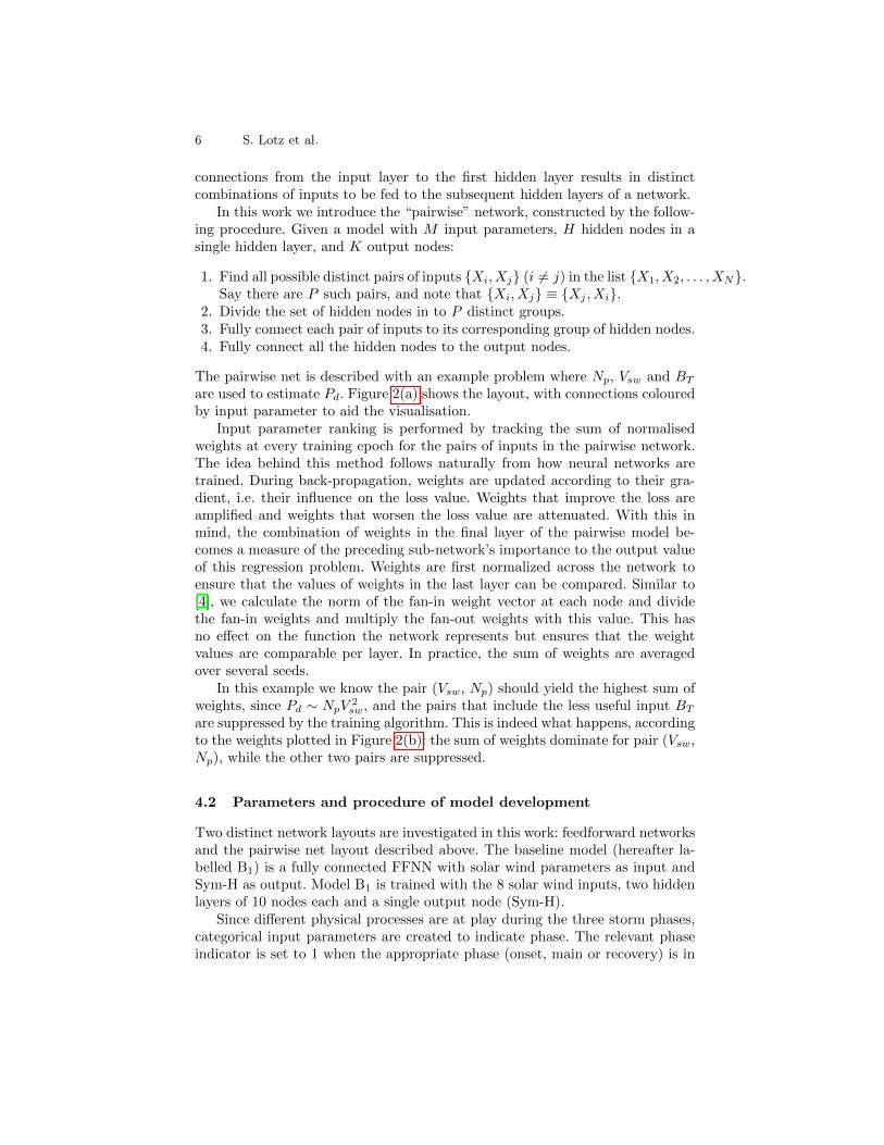
The pairwise net is described with an example problem where Np, Vsw and BT

are used to estimate Pd. Figure 2(a) shows the layout, with connections colouredby input parameter to aid the visualisation.

Input parameter ranking is performed by tracking the sum of normalisedweights at every training epoch for the pairs of inputs in the pairwise network.The idea behind this method follows naturally from how neural networks aretrained. During back-propagation, weights are updated according to their gra-dient, i.e. their influence on the loss value. Weights that improve the loss areamplified and weights that worsen the loss value are attenuated. With this inmind, the combination of weights in the final layer of the pairwise model be-comes a measure of the preceding sub-network’s importance to the output valueof this regression problem. Weights are first normalized across the network toensure that the values of weights in the last layer can be compared. Similar to[4], we calculate the norm of the fan-in weight vector at each node and dividethe fan-in weights and multiply the fan-out weights with this value. This hasno effect on the function the network represents but ensures that the weightvalues are comparable per layer. In practice, the sum of weights are averagedover several seeds.

In this example we know the pair (Vsw, Np) should yield the highest sum ofweights, since Pd ∼ NpV

2sw, and the pairs that include the less useful input BT

are suppressed by the training algorithm. This is indeed what happens, accordingto the weights plotted in Figure 2(b): the sum of weights dominate for pair (Vsw,Np), while the other two pairs are suppressed.

4.2 Parameters and procedure of model development

Two distinct network layouts are investigated in this work: feedforward networksand the pairwise net layout described above. The baseline model (hereafter la-belled B1) is a fully connected FFNN with solar wind parameters as input andSym-H as output. Model B1 is trained with the 8 solar wind inputs, two hiddenlayers of 10 nodes each and a single output node (Sym-H).

Since different physical processes are at play during the three storm phases,categorical input parameters are created to indicate phase. The relevant phaseindicator is set to 1 when the appropriate phase (onset, main or recovery) is in


(a) Pairwise network layout. Thedouble-headed arrows indicate full con-nection (for picture clarity).

(b) Weight evolution over 10 epochs oftraining.

Fig. 2. Pairwise network with three inputs and one output. Dynamic pressure Pd ispredicted by three parameters, BT , Vsw and Np, while it is known that only two ofthem are useful (Vsw and Np).

progress, and set to 0 at other times. Therefore, model B2 has 8 + 3 = 11 inputparameters.

A further improvement is made by adding temporally shifted versions of eachparameter to the set of inputs. For each input parameter Xt, measured at timet, another input Xt−m is added, doubling the number of inputs of model B3

to 16. The magnetosphere has a measure of “memory” in that the magneto-hydrodynamic processes that govern the storm time phenomena take some timeto react and recover from solar wind energy input [12]. In this case we letm = 270minutes, chosen by a parametric search of shifts. Applying this time shift resultedin a marked increase in performance (see Section 5).

Various pairwise network models are developed. A simple model with the 8solar wind inputs and 10 hidden nodes in 2 hidden layers is trained (P1), andis shown to perform as well as model B1. This shows that the pairwise nodesdo not reduce performance for this application. Subsequent pairwise models aredeveloped by adding phase and time-shifted parameters (P2 and P3).

Both the Bi and Pi models are trained with Adam as the optimizer andmean squared error as the loss function. Correlation between the predicted andobserved output is used as a performance metric. All optimization decisions arebased on the model’s performance on the validation set. Early stopping is im-plemented by selecting models with the largest validation correlation. Extensiveprobing showed that weight decay, batch normalization and learning rate sched-ulers make little to no improvement to the performance, therefore none of theseare used. It was also found that smaller mini-batches have better performance,so a mini-batch size of 64 is chosen. Increasing the network width or depth doesnot improve performance, therefore the mentioned network sizes are chosen assuch in favour of computational efficiency. A grid search is done to determinethe best learning rate. Three initialization seeds are considered for both the Bi

8 S. Lotz et al.

and the Pi models. The test results of these models are listed in Table 1 anddiscussed in the next section.

5 Results

5.1 Baseline model

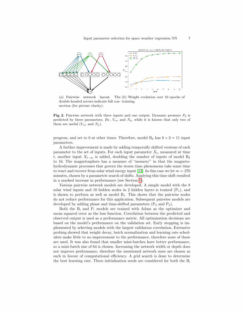
Without phase or time-shifted inputs, the optimal baseline model (B1) has a0.63 test correlation. By adding phase (B2) or time-shifted inputs (B3), theperformance increases to 0.79 and 0.76, respectively. With both phase and time-shifted inputs added (B4), the model reaches a test correlation of 0.83.

Figure 3 shows an example of Sym-H predicted by models B1 and B4 duringa geomagnetic storm. It clearly shows the advantage of adding phase informationand time-shifted parameters to the set of inputs, especially during the onset andrecovery phases.

Table 1. Model performance for the different model types.

Model Description Layout Test Corr. S.E.

B1 FFNN 8:(10,10):1 0.63 0.0008B2 FFNN with phase (8+3):(10,10):1 0.79 0.0081B3 FFNN with time-shifted inputs (8+8):(10,10):1 0.76 0.0100B4 FFNN with phase and t-shifted inputs (8+3+8+3):(10,10):1 0.83 0.0047P1 Pairwise net 8:(10,10)a:1 0.66 0.0066P2 Pairwise net with phase (8+3):(10,10)a:1 0.81 0.0022P3 Pairwise net with time-shifted inputs (8+8):(10,10)a:1 0.77 0.0022P4 Pairwise net with phase and t-shift (8+3+8+3):(10,10)a:1 0.81 0.0056

a Hidden layers of the pairwise model’s sub-networks

5.2 Pairwise net

With no phase information or time-shifted inputs (P1), the best model has a 0.66correlation on the test set. By adding phase (P2) or time-shifted (P3) inputs, thevalidation correlation increases to 0.81 and 0.77, respectively. With both phaseand time-shifted (P4) inputs, the test correlation is 0.81.

5.3 Input parameter ranking through pairwise net

The pairwise net P1 is developed with (i) the entire data set, and (ii) with thedataset divided according to the three storm phases. This enables the ranking ofinput pairs in general and for separate storm phases. This is to see if the inputranking via the pairwise nets reflects the known differences in physical phenom-ena at play during the different storm phases. In both cases the best performing


��

��

��

��

��

��

��

��

��

��

��

��

��

��

�

�

�

��

Fig. 3. Predicted and observed Sym-H values during a geomagnetic storm. Model pre-diction results are shown both with and without phase and time-shifted inputs. Thedifferent storm phases are also indicated here.

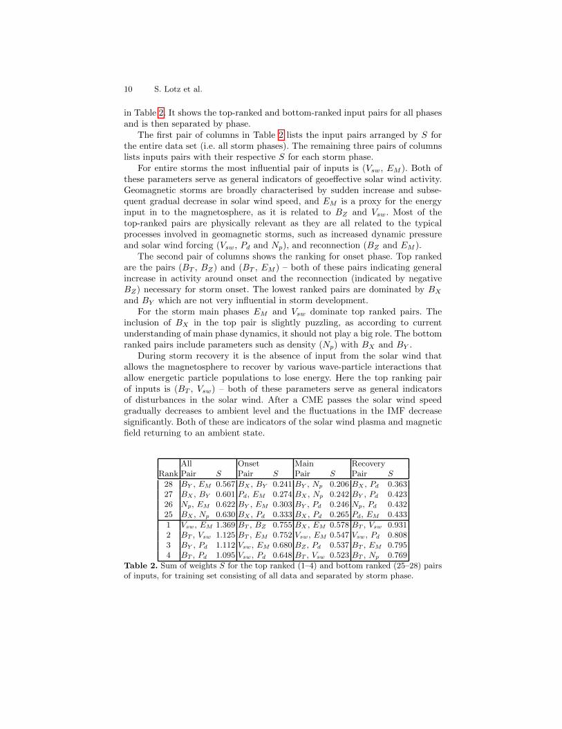
pairwise model is used. Ranking is done by taking the sum of absolute normalizedweights on the epoch where the model achieved its best validation performance.The results are then averaged over 4 iterations with different initialization seeds.All 8 input parameters are considered in pairs of 2. Table 2 shows the resultingaverage sum S of absolute normalized weights after the last epoch, for the topranked and bottom ranked input pairs.

6 Discussion and Conclusions

6.1 Model performance

This investigation confirms that neural networks are a viable option for predict-ing a geomagnetic storm index (i.e. Sym-H) only from solar wind parameters.The simplest model are able to reach a test correlation of 0.63. By adding phaseand temporal information, the performance increases to 0.83.

The proposed pairwise network achieved approximately the same predictiveperformance as the simple baseline neural network, with the added benefit ofranking the importance of input parameters.

6.2 Interpretation of the input parameter selection

The pairwise nets enable a crude form of input parameter ranking, built in tothe framework of a fully connected FFNN, without the need for explicit rankingprocedures. The sum of absolute normalized weights S at the final epoch is listed

10 S. Lotz et al.

in Table 2. It shows the top-ranked and bottom-ranked input pairs for all phasesand is then separated by phase.

The first pair of columns in Table 2 lists the input pairs arranged by S forthe entire data set (i.e. all storm phases). The remaining three pairs of columnslists inputs pairs with their respective S for each storm phase.

For entire storms the most influential pair of inputs is (Vsw, EM ). Both ofthese parameters serve as general indicators of geoeffective solar wind activity.Geomagnetic storms are broadly characterised by sudden increase and subse-quent gradual decrease in solar wind speed, and EM is a proxy for the energyinput in to the magnetosphere, as it is related to BZ and Vsw. Most of thetop-ranked pairs are physically relevant as they are all related to the typicalprocesses involved in geomagnetic storms, such as increased dynamic pressureand solar wind forcing (Vsw, Pd and Np), and reconnection (BZ and EM ).

The second pair of columns shows the ranking for onset phase. Top rankedare the pairs (BT , BZ) and (BT , EM ) – both of these pairs indicating generalincrease in activity around onset and the reconnection (indicated by negativeBZ) necessary for storm onset. The lowest ranked pairs are dominated by BX

and BY which are not very influential in storm development.For the storm main phases EM and Vsw dominate top ranked pairs. The

inclusion of BX in the top pair is slightly puzzling, as according to currentunderstanding of main phase dynamics, it should not play a big role. The bottomranked pairs include parameters such as density (Np) with BX and BY .

During storm recovery it is the absence of input from the solar wind thatallows the magnetosphere to recover by various wave-particle interactions thatallow energetic particle populations to lose energy. Here the top ranking pairof inputs is (BT , Vsw) – both of these parameters serve as general indicatorsof disturbances in the solar wind. After a CME passes the solar wind speedgradually decreases to ambient level and the fluctuations in the IMF decreasesignificantly. Both of these are indicators of the solar wind plasma and magneticfield returning to an ambient state.

All Onset Main RecoveryRank Pair S Pair S Pair S Pair S

28 BY , EM 0.567 BX , BY 0.241 BY , Np 0.206 BX , Pd 0.36327 BX , BY 0.601 Pd, EM 0.274 BX , Np 0.242 BY , Pd 0.42326 Np, EM 0.622 BY , EM 0.303 BY , Pd 0.246 Np, Pd 0.43225 BX , Np 0.630 BX , Pd 0.333 BX , Pd 0.265 Pd, EM 0.433

1 Vsw, EM 1.369 BT , BZ 0.755 BX , EM 0.578 BT , Vsw 0.9312 BT , Vsw 1.125 BT , EM 0.752 Vsw, EM 0.547 Vsw, Pd 0.8083 BY , Pd 1.112 Vsw, EM 0.680 BZ , Pd 0.537 BT , EM 0.7954 BT , Pd 1.095 Vsw, Pd 0.648 BT , Vsw 0.523 BT , Np 0.769

Table 2. Sum of weights S for the top ranked (1–4) and bottom ranked (25–28) pairsof inputs, for training set consisting of all data and separated by storm phase.


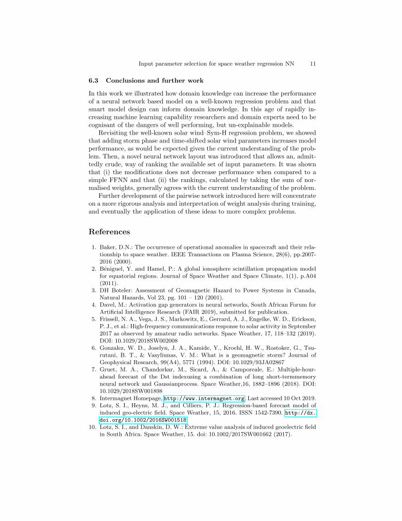
6.3 Conclusions and further work

In this work we illustrated how domain knowledge can increase the performanceof a neural network based model on a well-known regression problem and thatsmart model design can inform domain knowledge. In this age of rapidly in-creasing machine learning capability researchers and domain experts need to becognisant of the dangers of well performing, but un-explainable models.

Revisiting the well-known solar wind–Sym-H regression problem, we showedthat adding storm phase and time-shifted solar wind parameters increases modelperformance, as would be expected given the current understanding of the prob-lem. Then, a novel neural network layout was introduced that allows an, admit-tedly crude, way of ranking the available set of input parameters. It was shownthat (i) the modifications does not decrease performance when compared to asimple FFNN and that (ii) the rankings, calculated by taking the sum of nor-malised weights, generally agrees with the current understanding of the problem.

Further development of the pairwise network introduced here will concentrateon a more rigorous analysis and interpretation of weight analysis during training,and eventually the application of these ideas to more complex problems.

References

1. Baker, D.N.: The occurrence of operational anomalies in spacecraft and their rela-tionship to space weather. IEEE Transactions on Plasma Science, 28(6), pp.2007-2016 (2000).

2. Beniguel, Y. and Hamel, P.: A global ionosphere scintillation propagation modelfor equatorial regions. Journal of Space Weather and Space Climate, 1(1), p.A04(2011).

3. DH Boteler: Assessment of Geomagnetic Hazard to Power Systems in Canada,Natural Hazards, Vol 23, pg. 101 – 120 (2001).

4. Davel, M.: Activation gap generators in neural networks, South African Forum forArtificial Intelligence Research (FAIR 2019), submitted for publication.

5. Frissell, N. A., Vega, J. S., Markowitz, E., Gerrard, A. J., Engelke, W. D., Erickson,P. J., et al.: High-frequency communications response to solar activity in September2017 as observed by amateur radio networks. Space Weather, 17, 118–132 (2019).DOI: 10.1029/2018SW002008

6. Gonzalez, W. D., Joselyn, J. A., Kamide, Y., Kroehl, H. W., Rostoker, G., Tsu-rutani, B. T., & Vasyliunas, V. M.: What is a geomagnetic storm? Journal ofGeophysical Research, 99(A4), 5771 (1994). DOI: 10.1029/93JA02867

7. Gruet, M. A., Chandorkar, M., Sicard, A., & Camporeale, E.: Multiple-hour-ahead forecast of the Dst indexusing a combination of long short-termmemoryneural network and Gaussianprocess. Space Weather,16, 1882–1896 (2018). DOI:10.1029/2018SW001898

8. Intermagnet Homepage, http://www.intermagnet.org. Last accessed 10 Oct 2019.9. Lotz, S. I., Heyns, M. J., and Cilliers, P. J.: Regression-based forecast model of

induced geo-electric field. Space Weather, 15, 2016. ISSN 1542-7390. http://dx.doi.org/10.1002/2016SW001518.

10. Lotz, S. I., and Danskin, D. W.: Extreme value analysis of induced geoelectric fieldin South Africa. Space Weather, 15. doi: 10.1002/2017SW001662 (2017).

12 S. Lotz et al.

11. Lotz, S., Heilig, B., and Sutcliffe, P.: A solar-wind-driven empirical model of Pc3wave activity at a mid-latitude location. Annales Geophysicae, 33, 225–234, 2015.DOI:10.5194/angeo-33-225-2015.

12. Moldwin, M.: An Introduction to Space Weather, Cambridge University Press(2008).

13. Oughton, E. J., Hapgood, M., Richardson, G. S., Beggan, D., Thomson, A. W.P., Gibbs, M., Horne, R. B. (2018). A Risk Assessment Framework for the Socioe-conomic Impacts of Electricity Transmission Infrastructure Failure Due to SpaceWeather: An Application to the United Kingdom. Risk Analysis, (November).https://doi.org/10.1111/risa.13229

14. Pecasus, http://pecasus.eu/. Last accessed 10 Oct 2019.15. Siscoe, G., McPherron, R. L., Liemohn, M. W., Ridley, A. J., & Lu, G.: Reconciling

prediction algorithms for Dst. Journal of Geophysical Research: Space Physics,110(December 2004), 1–8. DOI: 10.1029/2004JA010465

16. Trichtchenko, L., & Boteler, D. H.: Modelling of geomagnetic induction in pipelines.Annales Geophysicae, 20(7), 1063–1072 (2002). DOI: 10.5194/angeo-20-1063-2002

17. P Wintoft, Wik, M., Lundstedt, H., Eliasson, L.: Predictions of local ground ge-omagnetic field fluctuations during the 7–10 November 2004 events studied withsolar wind driven models. Ann. Geophys. 23, 3095–3101 (2005).

18. OMNIWeb Homepage, https://omniweb.gsfc.nasa.gov/. Last accessed 10 Oct2019.

19. DSCOVR Homepage, https://www.nesdis.noaa.gov/content/

dscovr-deep-space-climate-observatory. Last accessed 10 Oct 2019.20. Advanced Composition Explorer, http://www.srl.caltech.edu/ACE/. Last ac-

cessed 10 Oct 2019.

Documents

Input parameter ranking for neural networks in a space