Embed Size (px)
Citation preview

INNEHÅLLSFÖRTECKNING/CONTENTSPage
Forssberg, Eric, Luleå University of Technology Energy in mineral beneficiation 1
Acarkan N., Kangal O., Bulut G., Önal G. Istanbul Technical University The comparison of gravity separation and flotation of gold and silver bearing ore 3
Ellefmo, Steinar & Ludvigsen, Erik, Norwegian University of Science and Technology Geological Modelling in a Mineral Resources Management Perspective 15
Hansson, Johan, Sundkvist, Jan-Eric, Bolin, Nils Johan, Boliden Mineral AB A study of a two stage removal process 25
Hulthén, Erik & Evertsson, Magnus, Chalmers University of Technology Optimization of crushing stage using on-line speed control on a cone crusher 37
Hooey1, P.L., Spiller2, D.E, Arvidson3, B.R., Marsden4, P., Olsson5, E.,1MEFOS, 2Eric Spiller Consultants LLC, 3Bo Arvidson Consulting LLC, 4, 5Northland Resources Inc. Metallurgical development of Northland Resources' IOCG resources 47
Ikumapayi, Fatai K., Luleå University of Technology, Sundkvist, Jan-Eric & Bolin, Nils-Johan, Boliden Mineral AB Treatment of process water from molybdenum flotation 65
Johansson, Björn, Boliden Mineral AB Limitations in the flotation process 79
Kongas, Matti & Saloheimo, Kari, Outotec Minerals Oy New innovations in on-stream analysis for flotation circuit management and control 89
Kuyumcu, Halit Z. & Rosenkranz, Jan, TU Berlin Investigation of Fluff Separation from Granulated Waste Plastics to be Used in 99Blast Furnace Operation
Mickelsson1, K-O, Östling2 J, Adolfsson3, G.,1LKAB Malmberget, 2Optimation AB Luleå, 3LKAB Kiruna New apatite flotation at Svappavaara 117
Sandvik, Knut L, NTNU & Norkyn, Paul Inge, Nordic Mining Processing of a world class rutile deposit in Norway 133
Thurley, Matthew, Luleå University of Technology Fragmentation Measurement in LHD Buckets using 3D Vision 145
Weihed, Pär, Luleå University of Technology Nordic Mining School (NMS) for Advanced Extractive technologyand Natural Resources Management 157
Wotruba1, H, Robben1, M, and Balthasar2, 1RWTH Aachen University, 2TiTech GmbH Near-Infrared Sensor-Based Sorting in the Minerals Industry 163


Energy in mineral processing.
By Eric Forssberg, Mineral Processing, LTU, SE 971 87 Lulea, Sweden
1. Introduction.
A first study on energy issues in mineral processing was made in the wake of the first oil crisis in 1973. The results have been published in a report from Statens Industriverk. A basic report has been issued by the Swedish Mining Association. The study was based on literature and information compiled from industry. Different mineral processing plants were analysed in detail regarding the energy consumption. For a plant like Aitik with low grade copper ore the comminution, especially the grinding is a dominating unit operation. About half of the electrical power was consumed by the grinding. In other cases like iron ore plants flotation and transportation is dominating. Often the energy needed for heating of buildings accounted for as thermal energy as GWh is much higher than the electrical power need for the process itself. It is well known that transportation consumes a large proportion of the energy. This is especially significant in the aggregates industry. Front end loaders and trucks use diesel oil while the process itself dominated by crushing and screening is fairly efficient.
Another study on energy in mineral processing and mining was undertaken in 2007 as part of a larger project within Jernkontoret called “Energihandboken”, www.energihandbok.se . The emphasis, of course is on the steel industry but there is one chapter on the mining industry. The study on the mining industry is based on literature and detailed surveys made for different plants by consultants on behalf of the mining companies. Consultants like Vattenfall Power Consultant and ÅF – Process AB have made the surveys.
A foreign document has been obtained from Rio Tinto “Energy and climate change – Challenges and opportunities for the mining industry” 2007, R Batterham and C Goodes. Valuable input was obtained from the Mining Association of Canada. “Benchmarking the energy consumption of Canadian open pit mines” and “Benchmarking the energy consumption of Canadian underground mines”, both in 2005.
2. How to save energy or increase the efficiency.
There are many ways to decrease the specific energy consumption:
-New technology -Control of processes and unit operations -Material technology.
Comminution is often regarded as the most important area for new technology. The energy efficiency of comminution is considered to be low. The frequently cited figure of 1 % energy efficiency is nonsense. However rotary mills consume a lot of power for tumbling of balls, rods or rocks. Much of this is converted into low grade heath. If tumbling mills are compared with other types like vertical mills or HPRM a figure for the energy efficiency at 30 à 50 % can be calculated. An increased use of the latter type of mills is hindered by the lack of suitable wear materials, especially for vertical mills.
1

New technologies like the Selfrag are slowly developing to large capacities. However this technology may rather do a better grinding job than save energy. The Australian development towards the Isamill” and others represent a significant step forward.Fine grinding, or regrinding of concentrates can be undertaken at fairly low specific energy consumption. A similar development has taken place in the industrial minerals industry except that the wish to maintain technology as proprietary is an issue.The tumbling mills have developed towards much better efficiency through the application of simulation methods leading to better design. This is an example of stepwise progress rather than the revolutionary development many people are looking for. In this context the ideas of Evertsson regarding crushing to a finer size can be mentioned. Crushing in terms of specific energy consumption is always more efficient than grinding in tumbling mills.
Materials technology, especially for wear resistant parts has been mentioned and its significance cannot be overemphasised. Wear of steel not only represents a cost but also the embedded energy for the production of the alloys and the steel. Sometimes simple solutions are to be preferred. The use of studs in HPRG can be mentioned.
Besides comminution sorting, flotation and dewatering are areas where the specific energy consumption has decreased.
In the area of control I believe that many of the simple solutions now have been applied. Those may be control of the RPM of fans and pumps and electrical engineering.
Thermal processes are becoming more and more efficient. The work within MinFo regarding applied mineralogy for limestone calcining can be mentioned. An increased yield in the lime burning will automatically give decreased specific energy consumption. The pioneering work in iron ore pelletizing within LKAB to develop highly efficient processes is well known.
3. Conclusions
The energy consumption is one important factor within the larger area “Sustainability”. Others are water and land. An interesting overview of this area was provided by Wotruba at the XXIV International Mineral Processing Congress in September 2008. The technology platform developed for the European Commission has the name Sustainable Mineral Resources and further European moves in this area can be expected.
2

THE COMPARISON OF GRAVITY SEPARATION AND FLOTATION ON GOLD AND
SILVER BEARING ORE
Ne et Acarkan, Olgaç Kangal, Gülay Bulut, Güven Önal
Istanbul Technical University, Faculty of Mines, Mineral Processing Department, 34469, Maslak-
ISTANBUL
ABSTRACT
Gold and silver are usually found in native form or in sulphide and silicate minerals and as
tellurides in nature. Placer and paleo-placer type of gold and silver ores are easily treatable and gold
and silver could simply be recovered by gravimetric concentration and flotation methods. In
refractory type ores, gold and silver are usually associated with sulphide minerals. Today, gold and
silver are usually recovered from metallic ores by chemical processes. Gravity concentration and
flotation being one of main processes could be used for pre-concentration and in combination with
chemical processes depending on the ore formation conditions.
In this study, concentrates were produced from gold and silver bearing ores taken from Bolkarda ,
Ni de region of Turkey by using gravity techniques and flotation according to the optimum
separation conditions. At the end of the evaluation of mineralogical and chemical results, shaking
table and flotation were used for concentration.
According to the concentration results performed with different particle sizes, a highly grade of
concentrate was obtained as 235 ppm Au, 3740 ppm Ag and 50,60% Pb content by using flotation.
1. Introduction
Gold and silver are usually found in native form or in sulphide and silicate minerals and as
tellurides in nature. Placer and paleo-placer type of gold and silver ores are easily treatable and gold
and silver could simply be recovered by gravimetric concentration methods. In refractory type ores,
gold and silver are usually associated with sulphide minerals (pyrite, arsenopyrite, marcasite,
pyrrhotite, chalcopyrite, orpiment, realgar, stibnite, etc.). Today, precious metals such as gold and
silver are usually recovered from metallic ores by chemical processes. Gravity concentration being
one of main processes could be used in combination with chemical processes depending on the ore
3

formation conditions (Allan and Woodcock, 2001, Hendriks and Chevalier, 2004, Laplante, 2001,
Meza et al., 2004, Wotruba and Müller, 2001).
Gold concentration processes usually consist of gravity separation, flotation, cyanidation or a
combination of these processes. Actually, the choice of those processes depends on the
mineralogical characterization and gold content of the ore. Gravitational gold recovery has
developed significantly for twenty five years, because of developing new gravitational techniques.
There are different types of gravity concentration devices have been developed. The most important
ones are Knelson, Falcon and Knudsen gravity concentrators and Mozley gravity separators.
Although there are different types of gravity separators, their concentration characteristics are
decreasing depending on the particle size (in the range of 50-500 microns). Gravity concentrators
such as Spiral, Shaking Table, Knelson Concentrator, Falcon Concentrator and Multi-Gravity
Separator are effectively used in the concentration of finely liberated ores.
Free metallic gold can be recovered very effectively by flotation and gravity methods. The most
common gold bearing sulphides are pyrite, arsenopyrite and pyrrhotite. In placer or gravity
concentrate treatment most the gangue minerals are oxides and silicates which are hydrophilic, and
strong collectors can be used to maximize gold recovery with little concern for co-recovery of
sulphides. This type of flotation is rare but has been proposed for low grade ores where gold is too
fine to be recovered by flotation.
The aim of this study is comparison gravity separation and flotation on recovery of gold bearing
ore.
2. Material and Methods
The complex lead and zinc ore used in this study were taken from Bolkarda , Ni de region of
Turkey. According to the mineralogical studies, the representative ore sample contains primarily
native gold, native silver, electrum and argentojarosite as gold and silver minerals, cerusite,
anglesite, galena, pyromorphite, mimetite and plumbojarosite as lead minerals, smithsonite,
hydrozincite, hemimorphite, adamite and sphalerite as zinc minerals, limonite, hematite, goethite,
pyrite, magnetite and siderite as lead minerals and quartz, feldspar, albite and muscovite as gangue
minerals. Chemical analysis of the representative ore sample is given in Table 1. Microscopic
images of the minerals in the ore compound are shown in Figures 1, 2, 3 and 4.
4

Table 1.Chemical Analysis of the Representative Ore Sample
Compound Content
Au, g/t 12,2
Ag, g/t 256
Fe2O3, % 40,47
Pb, % 3,45
Zn, % 3,15
Cu, % 0,11
SiO2, % 29,09
MgO, % 0,81
CaO, % 3,53
Al2O3, % 3,01
Na2O, % 0,09
K2O, % 0,56
TiO2, % 0,14
P2O5, % 0,10
MnO, % 1,24
Loss on Ignition, % 13,90
According to the mineralogical analyses, gold, silver and lead minerals partially liberated below
300 microns. Therefore, shaking table experiments were performed with -300 microns particle size.
Wilfley type shaking table were used in gravity experiments. Flotation experiments performed with
-38 microns were carried out Denver type flotation unit. Aminotiophenol (ATP-C6H7NS) and
potassium amyl xanthate (CH3CH2CH2CH2CH2OCS2K) as collectors, Na2SiO3 as depressant, Na2S
as sulphidized reagent and methyl isobutyl Carbinol (MIBC) as frother were used in flotation.
5

Figure 1. Native gold particles (au) in Figure 2. Native gold particles (au) inhematite (he) and gothite (gö) hematite (he)
Figure 3. Native gold (au) particles together Figure 4. Native gold (au) particles together with cerusite (se), mimetite (mi) and with cerusite (se), mimetite (mi) andplumbojarosite (pj) particles plumbojarosite (pj) particles
6

3. Results and Discussion
3.1 Gravity separation experiments
Representative ore sample was ground under 300 microns particle size for shaking table
experiments. -300 microns sample was classified as -300+150 microns and -150 microns. These
particle size groups were fed onto shaking table. During the experiments, products were tried to
take as narrow stripes. Middlings were recycled onto shaking table for three times, then combined
in respect of their mineralogical contents and final concentrate, middlings and tailings were
produced. The results of shaking table experiments are given in Tables 2, 3, 4 and 5.
At the end of the shaking table experiments performed with -300 microns particle sizes, a lead
concentrate having 61,86% Pb, 202,6 ppm Au and 2232 ppm Ag was obtained. This concentrate is a
marketable product. Metal recoveries were shown as 13,5% for gold, 6,5% for silver and 15,2% for
lead. Silver concentration recovery is less than the other metals because of argentojarosite. This
mineral can easily disintegrate and mix to slime. Valuable metal losses in the slime are not less than
25%. Therefore, Au contents in tailings could not be reduced under 8,5-9 ppm.
3.2 Flotation experiments
After grinding under 38 microns particle sizes of the representative ore sample, multi-staged
flotation experiments were performed on it. While natural pulp pH was 8,5, it increased to 9,85 by
addition of Na2S. Flotation experimental conditions, experimental flowsheet and results are given in
Table 6, Figure 5 and Table 7, respectively.
7

Table 6. Flotation Experimental Conditions
Na2SiO3 1000 g/t
3000 (1000+1000+1000) g/t (First 3 steps)
2000 (500+500+500+500) g/t (Next 4 steps) Na2S
600 g/t (Final steps)
300 (100+100+100) g/t (First 3 steps)
200 (50+50+50+50) g/t (Next 4 steps) ATP
100 g/t (Final steps)
300 (100+100+100) g/t (First 3 steps)
200 (50+50+50+50) g/t (Next 4 steps) KAX
100 g/t (Final steps)
MIBC 20+20 g/t
Na2SiO3 Conditioning Time 10 minutes
Na2S Conditioning Time 3+3+3+3+3+3+3 minutes
ATP+KAX Conditioning Time 5+5+5+5+5+5+5+5 minutes
Flotation Time 2,5+2,5+2,5+2,5+2,5+2,5+2,5+2,5 minutes
Cleaning Stages Conditioning Times 2+2+2 minutes
Cleaning Stages Flotation Times 5+5+5 minutes
8

Tabl
e 2.
Au,
Ag,
Pb
and
Zn F
ract
iona
l Ana
lysi
s Res
ults
of -
300
mic
rons
Au
Ag
PbZn
Parti
cle
Size
,
mic
ron
Am
ount
,
%C
onte
nt, p
pm
Rec
over
y, %
C
onte
nt, p
pm
Rec
over
y, %
C
onte
nt, %
R
ecov
ery,
%C
onte
nt, %
Rec
over
y, %
-300
+150
24,0
11,3
22,8
215
18,7
3,21
23,7
3,24
23,3
-150
+ Sl
ime
53,2
11,8
52,8
275
53,1
3,08
50,3
3,31
52,9
Slim
e 22
,812
,724
,434
028
,23,
7126
,03,
4823
,8
Tota
l10
0,0
11,9
100,
027
510
0,0
3,25
100,
03,
3310
0,0
Tabl
e 3.
Sha
king
Tab
le E
xper
imen
tal R
esul
ts (A
ccor
ding
to th
e Ex
perim
ent)
Au
Ag
PbZn
Parti
cle
Size
,
mic
ron
Prod
ucts
Am
ount
,
%C
onte
nt,
ppm
Rec
over
y,
%
Con
tent
,
ppm
Rec
over
y,
%
Con
tent
,
%
Rec
over
y,
%
Con
tent
,
%
Rec
over
y,
%
Con
cent
rate
1,3
129,
914
,923
0514
,054
,28
22,0
2,33
0,9
Mid
dlin
gs47
,410
,945
,723
952
,83,
6253
,44,
0659
,5
Taili
ngs
51,3
8,7
39,4
139
33,2
1,54
24,6
2,50
39,6
-300
+150
Tota
l10
0,0
11,3
100,
021
510
0,0
3,21
100,
03,
2410
0,0
Con
cent
rate
0,9
246,
218
,8
2188
7,2
66,4
019
,40,
800,
2
Mid
dlin
gs19
,712
,020
,0
485
34,8
4,64
29,6
3,86
23,0
Taili
ngs
79,4
9,1
61,2
20
158
,01,
9851
,03,
2076
,8-1
50+S
lime
Tota
l10
0,0
11,8
100,
0
275
100,
03,
0810
0,0
3,31
100,
0
9

Tabl
e 4.
Sha
king
Tab
le E
xper
imen
tal R
esul
ts (A
ccor
ding
to th
e Fe
ed)
Au
Ag
PbZn
Parti
cle
Size
,
mic
ron
Prod
ucts
Am
ount
,
%C
onte
nt,
ppm
Rec
over
y,
%
Con
tent
,
ppm
Rec
over
y,
%
Con
tent
,
%
Rec
over
y,
%
Con
tent
,
%
Rec
over
y,
%
Con
cent
rate
0,3
129,
93,
323
052,
654
,28
5,1
2,33
0,2
Mid
dlin
gs11
,410
,910
,523
99,
93,
6212
,74,
0613
,9-3
00+1
50
Taili
ngs
12,3
8,7
9,0
139
6,2
1,54
5,9
2,50
9,2
Con
cent
rate
0,5
246,
210
,221
883,
966
,40
10,1
0,80
0,1
Mid
dlin
gs10
,512
,010
,548
518
,44,
6414
,83,
8612
,2-1
50+S
lime
Taili
ngs
42,2
9,1
32,1
201
30,8
1,98
25,4
3,20
40,6
Slim
e 22
,812
,724
,434
028
,23,
7126
,03,
4823
,8
TOTA
L10
0,0
11,9
100,
027
510
0,0
3,27
100,
03,
3310
0,0
Tabl
e 5.
Sha
king
Tab
le E
xper
imen
tal R
esul
ts (C
ombi
ned
with
Cal
cula
tion)
Au
Ag
PbZn
Parti
cle
Size
,
mic
ron
Prod
ucts
Am
ount
,
%C
onte
nt,
ppm
Rec
over
y,
%
Con
tent
,
ppm
Rec
over
y,
%
Con
tent
,
%
Rec
over
y,
%
Con
tent
,
%
Rec
over
y,
%
Con
cent
rate
0,8
202,
613
,522
326,
561
,86
15,2
1,37
0,3
Mid
dlin
gs21
,911
,421
,035
728
,34,
1127
,53,
9626
,1
Taili
ngs
54,5
9,0
41,1
187
37,0
1,88
31,4
3,04
49,8
Slim
e 22
,812
,724
,434
028
,23,
7125
,93,
4823
,8
-300
Tota
l10
0,0
11,9
100,
027
510
0,0
3,27
100,
03,
3310
0,0
10

Cleaning Step-3
Final Concentrate
Middlings-3
Middlings-2
Middlings-1
Tailings
Cleaning Step-1
Cleaning Step-2
RougherConcentrate
Grinding
3 Steps Flotation
4 Steps Flotation
1 Step Flotation
Figure 5. Experimental Flowsheet
11

Table 7. Results of Experiments Performed with Optimized Conditions
Au Ag Pb
ProductsAmount
%Content,
ppm
Recovery,
%
Content,
ppm
Recovery,
%
Content,
%
Recovery,
%
Concentrate 2,7 235,0 52,5 3740 37,6 50,60 39,7
Tailings 97,3 5,9 47,5 172 62,4 2.13 60,3
Total 100,0 12,1 100,0 268 100,0 3,44 100,0
As it is seen from Table7, a concentrate having 50,60% Pb was obtained with 39,7% recovery.
Also, this concentrate contains 235 ppm Au and 3740 ppm Ag. At the end of these tests, it was
found that the addition of KAX and ATP was highly affected on the flotation of gold and silver
minerals such as treated of oxidized lead minerals.
4. Conclusions
It was determined that the complex lead-zinc ore sample containing 3,45% Pb, 3,15% Zn, 12,2
g/t Au and 256 g/t Ag.
According to the mineralogical studies, the representative ore sample contains primarily native
gold, native silver, electrum and argentojarosite as gold and silver minerals, cerusite, anglesite,
galena, pyromorphite, mimetite and plumbojarosite as lead minerals, smithsonite, hydrozincite,
hemimorphite, adamite and sphalerite as zinc minerals, limonite, hematite, goethite, pyrite,
magnetite and siderite as lead minerals and quartz, feldspar, albite and muscovite as gangue
minerals.
In shaking table experiments performed with -300 microns, a concentrate having 202,6 ppm Au,
2232 ppm Ag, 61,86% Pb contents was obtained with 13,5% Au, 6,5% Ag and 15,2%
recoveries.
Multi-stage flotation experiments performed with KAX and ATP collectors (Optimum
conditions: 5000 g/t Na2S, 1000 g/t Na2SiO3, 500 g/t KAX, 500 g/t ATP, 40 g/t MIBC) showed
that a marketable concentrate having 235 ppm of Au, 3740 ppm of Ag and 50,60% Pb contents
was obtained with 52,5% Au, 37,6% Ag and 39,7% Pb recoveries.
12

5. References
Allan, G. C. and Woodcock, J. T., A Review of the Flotation of Native Gold and Electrum,
Minerals Engineering, Vol. 14, No. 9, pp. 931-962, (2001)
Hendriks, D. W. and Chevalier, G., Recovery of Gold Using Gravity Concentration the Hemlo
Experience, website of www.knelson.com, (2004)
Laplante, A. R., Report on the Characterization of Gravity Recoverable Gold in a Sample of
Kemess #1 Ore, Technical Report, McGill University, January, (2001)
Meza, L. A., Hartmann, W., Escobar, C., Recovery of Placer Gold Using the Knelson Concentrator,
website of www.knelson.com, (2004)
Wotruba, H.; Müller, W., Dichtesortierung von primären Golderzen als Alternative zur Laugung,
Sortieren Innovationen und Anwendungen, Vortraege zum 2. Kolloqium Sortieren, 11. und 12.
Oktober 2001, Berlin, S. 169-176
13

14

Geological Modelling in a Mineral Resource Management Perspective
Steinar L. Ellefmo 1*, Erik Ludvigsen 1Norwegian University of Science and Technology
Sem Sælandsv 1 7491 Trondheim
Norway
*Corresponding author: [email protected], tlf: +47 73 59 48 56
ABSTRACT
This paper defines Mineral Resource Management and illustrates how this management principle can be applied to increase the reserve base of a mining company. The geology model constitutes the actual foundation of all mining activities. A relatively new method to generate geology models is presented and applied on real data. The method makes it possible to generate, based on a vast amount of geological data, geology models fast and efficient. This makes it possible to test and evaluate different geological scenarios and how they can influence on the processing performance. Success in mining requires a strong link between geology and processing. Processing mineralogy constitutes a possible link between these two fields.
1. Introduction
“All models are wrong. Some models are useful.” (Box, 1979)
1.1 Background
The ultimate goal of any mining company is to make money. Investors require rapid payback, and with the recent international financial crisis in mind, the attitude towards project risks has changed.
1.2 Management and tools
Traditionally management is about getting people to work together to reach stated goals. It compromises activities like planning, organizing, directing and controlling an organisation. One can also talk about the management of physical objects like mineral resources or commercial properties. This would basically mean to exploit the inherent potential in objects.
Different tools or concepts have been developed to provide aid in performing the management activities. These include “mine-to-mill”, mining value chain and geometallurgy or geometallurgical mapping.
15

So called “Mine to mill” - improvements have an aim to improve the production chain from in situ raw material to saleable product. This is achieved by optimizing the chain as a whole instead of optimizing the different processes individually. Optimizing the chain as a whole on one side and optimizing each and every process individually on another is often, if not always, mutually exclusive.
Geometallurgical mapping is an integrated, team based approach to document ore variability and quantifying the impact of geology and mineralogy on grinding, metallurgical response and metal recovery processes.
The spatial database generated through the geometallurgical mapping activities can be integrated into a 3D block model and used actively in production planning activities.
Mine planning is performed in order to increase the probability that saleable products that conform with quality and quantity requirements to internal or external customers are delivered in time. The mining value chain concept is build upon an idea that it is possible to obtain competitive advantages by arranging value adding activities in a sequential chain. See Ellefmo (2005) and the references therein. According to the concept, the value chain can be arranged as a series of primary (and value adding) activities. The chain consists in addition to the primary activities of controlling- and supporting activities. The controlling activities are there to assure that the primary activities are performed according to procedures and the supporting activities are non-value adding activities necessary for the primary activities to be performed effectively.
The World Commission on Environment and Development (1987) defined sustainable development (SD) as a development that meets the needs of the present generation without compromising the ability of future generations to meet their needs. Sustainable development is founded on three pillars. These are environmental protection and economic- and social development. Shields and Solar (2004) see human- natural-, social- and human-made capital in relationship to these pillars and they define weak sustainable development as a development that keeps the total capital in a community constant. Strong sustainability is seen as a development where none of the capitals are reduced. None of these two types of sustainability is appropriate in a mining context. One must instead keep a holistic view and perhaps accept that not the same sustainability principles are applied everywhere.
16

1.3 Mineral Resource Management
Mineral Resources Management compromises a holistic, multi-disciplinary approach to maximise the value add along the mining value chain. It contains elements of all the concepts and tools above.
With Mineral Resource Management we understand a company’s management of the deposit or deposits the operation is based on. The geometric- and the qualimetric model of the deposit forms the very foundation for a sustainable, profitable and responsible exploitation of the deposit. This require
Geometric and qualimetric geological modelling to know the shape and quality of the deposit. Focus on environmental issues like emissions to air and water, depositing of waste rock material and reclamation Knowledge of legal issues. Planning, visualisation and communication of development- and operational plans. Communication with the authorities and local communities.
Figure 1 illustrates factors influencing the (dynamic) size of the reserve base of a mining company. These factors are geology, or geological knowledge, financial- and engineering aspects and accessibility. The factor “Accessibility” contains aspects like social licence to operate and to expand and aspects like land use conflicts.
Figure 1 Factors influencing the reserve base of a mining company.
17

Although the factors seem uncorrelated in Figure 1, it is a well known fact that the geology factor has a strong influence on the financial- and engineering aspects. Poor understanding of in situ ore variations and how these variations influence the recovery and the behaviour of the fragmented raw material in the processing plant will prevent the company to achieve the stated goals. See e.g. Lipton (2002)
2. Combined mining
Combined mining is co- and / or after-use of volumes or areas affected by mining or quarrying activities. In other words, using the voids produced through mining to other industrial activities such as
Waste disposal Storage facilities Car parks Power plants Recreation centres Fish farming Real estate development Facilities for water- or sewage purification
Some of these examples presuppose that the mining or quarrying activities have ceased and are taking place in or near urban areas.
In many parts of the world, mining related voids have been used after the mining activities have ceased, i.e. after-use. One example is SubTropolis beneath Kansas City, USA (Hunt Midwest 2006). Benardos et al. (2001) conclude that underground aggregate production mining in the Athens area with after-use of the voids is an attractive investment plan. Nielsen and Myrvang (199?) and Myrvang and Nielsen (2002) investigate how underground aggregate production can be combined with depositing of waste. However, co-use where the secondary activities are included in the plans on a feasibility stage or on an early production stage is to the author’s knowledge not so often encountered.
A focus on combined mining in cases where this is feasible will increase the probability of getting the social licence to operate and expand. The total reserve base will therefore increase, because more ore is made accessible.
3. Geological modelling
Describing the mineral resource is primarily a task for the geologist. Producing an estimate of the ore reserve requires a multi-disciplinary approach with tight collaboration between geologists, mining engineers, metallurgists, process engineers and financial specialists.
18

Every deposit is unique. This uniqueness will along with different challenges related to location, logistic and infra structure, define a unique set of mining and processing risks.
Basically, there are two ways to establish a three-dimensional geology model. Common for both of them, is that they need geodata. These two approaches are the explicit (traditional) approach and the implicit approach.
2.1 Explicit geological modellingExplicit geological modelling consists in constructing horizontal or vertical profiles based on borehole data and preferably surface maps showing the outcrops of the ore. These profiles can then, to add constrains or controlling elements to the model, be tied together using so-called tie- or control lines. A triangulation algorithm can thereafter be used to construct a three dimensional solid. Figure 2 show a geometric model of a plate-like base metal deposit. Such triangulation algorithms are implemented in most mining software.
Figure 2 A explicit geologic model of a plate like base metal deposit.
The traditional approach is tedious and it is rather difficult and cumbersome to update the model when new geodata is collected.
2.2 Implicit geological modellingAn implicit model of a solid is given by a volume function defined throughout space. The volume function is interpolated from geodata such as borehole data and / or outcrop maps. The surface of the solid can be extracted from the function. The surface is in other words not constructed directly, as in explicit modelling where wireframes are constructed from vertical or horizontal sections, and is therefore called an implicit model.
The problem is to approximate a real valued function f(x) by s(x) given e.g. n values (data) with coordinates xi, yi and zi, where i = 1,…, n.
19

To do this, s(x) is chosen to be on the form
n
iii xxxpxs
1Eq. 1
In Equation 1, p(x) is a polynomial of degree at most k, i is a real valued weight attached to each data point, is a basis function, e.g. (r) = r2 log(r) and |x-xi|is the Euclidian distance between data point i and the point to be estimated.
The interpolant s(x) is defined by the coefficients of p(x) and the weights i.Given the data points, the algorithm finds the coefficients of p(x) and the i so that s(x) approximates the data points under the requirement that
01
N
jjj xp Eq. 2
An important aspect of a surface extracted from an implicit model is that is has a positive and a negative side. This can be used in geotechnical or geological domaining.
Leapfrog™ is a software build to utilize the implicit modelling technique. The software uses the FastRBF™ engine, which makes handling of very large datasets possible.
More information on implicit modelling is given in Cowan et al. (2002 and 2003).
Implicit modelling can take any numeric data as input, e.g.:
• Lithology • Grades • Geotechnical data
Figure 3 shows a geometric model established with implicit geologic modelling. Input data has been interpreted structural trends, outcrop data and borehole data.
20

Figure 3 Implicit geometric model showing a structurally complex steeply dipping deposit.
Structural information can be implemented into the modelling process by using oriented search ellipsoids with axes and orientation given by geological trends. Structural data (strike and dip measurements) can also be implemented and taken directly into account in the modelling. Figure 4 shows such an example. The discs shown in the figure represent strike and dip measurements, taken directly into account in the modelling.
Figure 4 Qualimetric grade model based on grade and structural data.
2.3 Geometric and qualimetric modelsA geometric geological model is a model that indicates the shape and the size of a geological unit like an ore. A qualimetric model quantifies the quality variations inside the geometric model. Geostatistics is a toolbox often used to establish the qualimetric model.
21

With advances in computer strength and with the development of efficient simulation techniques (see e.g. Dimitrakopoulos et al. (2002)) it is now possible to simulate large ore bodies and to get a good idea of the variations in the run-of-mine (ROM) grade. This constitutes a valuable input into the planning, the designing and the development of the processing plant.
4. Link between geological modelling and mineral processing
Lipton (2002) calls for a better a link between geological modelling and mineral processing. He lists a number of examples down-under where this link at the best was weak. Common for all of his examples is that the projects failed to satisfy the stated goals. Also in Norway there are examples where millions have gone lost due to a missing link between the geology model and the mineral processing activities.
Grade is an important parameter and the geology model must quantify the grade variations. However, equally important is a parameter like specific gravity, which might have a dramatic effect on the tonnage estimates. Further, grinding properties and mineralogy that will affect the consumption of flotation agents are also of crucial importance.
The strength of a rock can be determined by using measurement while drilling (MWD) techniques, where the response from the rock on the drill bit is measured, stored and analysed. The strength of a rock has a great influence on the grinding properties. Michaux and Djordevic (2005) have studied the influence of explosive energy on the strength of the rock fragments and SAG Mill throughput. They conclude that blast fragmentation influences the performance of downstream processes in a mine, and as a consequence, the profit of the whole operation can be improved. They also emphasise that grinding performance can be assisted by altering the fragmentation induced from the blasting.
The industrial mineral sector of our industry is often faced with extreme quality requirements. Given this, it is of vital importance that the link between the geology model and saleable product is strong and that a multi-disciplinary approach is selected whenever a potential mining project is due to be evaluated.
5. DiscussionWith Leapfrog™ it is easy and fast to generate different models by using different, but realistic anisotropies, search ellipsoids or resolution. It is therefore possible to generate and evaluate different geological scenarios. These would be a result of subjective geological considerations, but once they are defined and documented, the generated model is an objective one. The transparency in the geology modelling process is thereby increased.
As new data is made available through geodata collection during mining, these data can be appended to the existing dataset and used to generate a new updated
22

geology model. This new model will in fact not be an updated version of the old model, but a completely new one conditioned on the new updated dataset.
Mineral resource management is a multi-disciplinary approach to the management of mineral resources. Different tools can be applied to aid in the management process. These tools can constitute the foundation of early warning systems that warn if the ROM-grade or other ore property deviates from the defined requirements.
3D geological modelling plays also an educational role. A well visualised ore body model can constitute a logic starting point for education of own personnel and in discussions between geologists, mining engineers and process engineers. The model is also well suited to illustrate the challenges the mining company is faced with for the public and local governments. This would aid in increasing the accessibility.
Not only visualisation of the ore body, but also visualisation in general, will help in increasing the accessibility.
6. ConclusionsImplicit modelling represents a new and promising way to establish geometric and qualimetric ore body models. Compared to the traditional way to establish such 3D-models the modelling approach is very fast. However, model validation has perhaps become even more important since more of the actual modelling is performed by the computer.
Processing mineralogy can be regarded as the link between geology model and processing performance, and the link must be taken seriously in order to reach stated goals.
23

7. ReferencesBenardos, A.G., Kaliampakos, D.C., Proisiotis, J.G., Mavrikos, A.A., Skoparantzos K.A. 2001. Underground aggregate mining in Athens: a promising investment plan. Tunnelling and Underground Space Technology. No. 16, pp 323-329.
Box, G. 1979. Robustness in the strategy of scientific model building. In: Launer, R.L., Wilkinson, G.N., (eds.) Robustness in statistics. New York (NY). Academic Press.
Cowan, E.J.; Beatson R.K.; Fright, W.R.; McLennan, T.J.; Mitchell, T.J. 2002. Rapid Geological modeling. Extended abstract for Applied Structural Geology for Mineral Exploration and Mining. International Symposium. Kalgoorlie, 23. – 25. September 2002.
Cowan, E.J.; Beatson R.K.; Ross, H.J.; Fright, W.R.; McLennan, T.J.; Evans, T.R.; Carr, J.C.; Lane, R.G.; Bright, D.V.; Gillman, A.J.; Oshust, P.A. and Titley, M. 2003. Practical Implicit Geological Modelling. 5th International Mining Geology Conference. 17. – 19. Nov. 2003, Bendigo, Victoria. Publication Series No 8/2003. The Australasian Institute of Mining and Metallurgy.
Dimitrakopoulos, R., Farrelly, C.T. and Godoy, M. 2002. Moving forward from traditional optimization: grade uncertainty and risk effects in open-pit design. Published in Trans. Instn. Min Metall (Sect. A: Min. tech) no. 111, January – April 2002.
Ellefmo, S. 2005. From deposit to product. A probabilistic approach to the value chain of iron ore mining. Doctoral Thesis. Norwegian University of Science and Technology. 271p.
Hunt Midwest 2006. Retrieved: Mai 14, 2006, from http://www.huntmidwest.com/subtropolis/index.html
Lipton, I. 2002. Geology, Metallurgy and Mining Engineering – Why We Must Strengthen the Links. Value Tracking Symposium. 7. – 8. October, Brisbane, Queensland, Australia. AusIMM. Pp 35-40.
Myrvang, A., Nielsen, K. 2001. Disposal of non-nuclear waste in underground caverns. In: proceedings, 28th ITA General Assembly and World Tunnel Congress. 28th ITA General Assembly and World Tunnel Congress, Sydney, Australia. 2002-03-02 - 2002-03-08
Nielsen, K., Myrvang, A. 199?. A holistic approach to mineral extraction and waste management in urban areas.
Shields, D. J. and Solar, S. V. 2004. Sustainable Mineral Resources Management and Indicatiors: Case Study Slovenia. Geological Survey of Slovenia, Ljubljana, 2004.
World Commission on Environment and Development. 1987. Our Common future. P. 398. UN. Oxford University Press.
24

A study of a two stage iron removal process
Johan Hansson 1, Jan-Eric Sundkvist 2, Nils-Johan Bolin 3 Boliden Mineral AB
SE-93681 Boliden Sweden 1, 2, 3
ABSTRACT A leaching process for base metals recovery often generates considerable amount of impurities such as iron and arsenic into the solution. It is a challenge to separate the non-valuable metals into manageable and stable waste products for final disposal, without loosing the valuable constituents. Boliden Mineral AB has patented a two-stage precipitation process that gives a very clean iron-arsenic precipitate by a minimum of coprecipitation of base metals. The obtained product has shown to have good sedimentation and dewatering properties, which makes it easy to recover the iron-arsenic depleted solution by filtration and washing of the precipitate.
1. Introduction Boliden Mineral AB has been working with the development of bioleaching processes since the beginning of 1960s. Some of Bolidens Complex Ore deposits in the “Skellefteå field” are of special interest when concerning the possible use of bioleaching techniques. A bioleaching solution often contains, apart from the valuable metals, some impurities as iron, antimony and arsenic. To be able to extract the valuable metals, in down stream processes, the solution has to be neutralised and the iron content has to be reduced. To meet the environmental requirements it is also important to know a way to produce a stable iron-arsenic end product. Boliden started the work with a selective precipitation process for iron removal in the beginning of 2000. At that time the existing iron removing process was not acceptable, especially with respect to the loss in zinc recovery from coprecipitation and also the handling of waste products. Therefore some work to develop a new method was initiated and a patent for a two-stage iron precipitation circuit was granted in 2002. This new method could achieve the desired level of metal recovery and waste product quality. This paper gives a presentation of the precipitation process together with some recent test work results, performed in the BioMine project (2004-2008).
25

2. The 2-stage iron removal circuit The two-stage iron removal process is based on a controlled neutralisation process using limestone, lime or any other similar alkaline material. A patent was granted June 18, 2002 (US 6,406,676 B1) [1], which describes a method for precipitation of iron and arsenic from multi-element solutions in a selective way. During the start of the test work it was found that when having an incomplete iron removal from the solution, there was a minimum of coprecipitation of valuable metals such as zinc and copper to the iron-gypsum precipitate. It was also shown that the incomplete iron removal results in a very dense and much more filterable precipitate compared to precipitates produced during a complete iron removal. Based on this observation the simplified flow sheet shown in Figure 1 was developed.
Figure 1. Simplified flow sheet of the 2-stage iron removal circuit.
The leach solution, which preferable contains ferric iron, is fed into the first precipitation stage. Recycled pulp from downstream apparatus is also fed into the first reactor in stage 1. The first stage consists of a number of reactors in series. The pH of the solution is raised step by step by controlled alkali addition. The partially neutralised solution from the last reactor in stage 1 discharges into the first thickener. At this point the solution will preferably contain a few hundreds milligrams of residual ferric per litre. The iron-gypsum precipitate is allowed to settle in the thickener without any addition of flocculant. The net percentage of iron removal in the first stage will depend on flowrate from recycled streams and concentration of residual ferric concentration in the overflow from thickener no. 1. The target is to remove as much iron as possible in the first precipitation stage. The net production of precipitate is discharged from thickener no. 1. The overflow from the first thickener is diverted to the first reactor of the secondary precipitation stage. The number of required reactors in the second stage is less than in the first stage since the pH control is not so critical. However, the overall retention time might be more of a critical issue in obtaining
Lime, limestone e t c to pH >2.2
Lime, limestone e t c to pH >3.0
Fe-free solution
Leach solution
Fe-gypsum to dump via filtration and washing
26

a high quality overflow from the secondary thickener. In the second stage the pH is raised to a level where the ferric iron and arsenate is completely removed from the leach solution. The pulp from the last reactor in stage 2 discharges into thickener no. 2, where the precipitate allows to settle. Flocculants are added to obtain a clear overflow, containing the valuable base metals for downstream processing. Some part of the valuable base metals might be coprecipitated in the second precipitation stage due to the relative high pH to be maintained for a complete removal of the iron. The precipitate will also contain some unreacted alkali. The second precipitate is therefore returned to the first reactor in the first precipitation stage. The lower pH in this stage ensures that any unreacted alkali is reused and any coprecipitated elements are dissolved. Other alkali additives can also be used, if available, and if they have sufficiently high reactivity. The temperature in the precipitation should preferably be as high as possible to get a good crystalline precipitate with good sedimentation and filtration properties. However, the temperature may in many cases be limited by the upstream conditions in an integrated bioleaching process unless external heat is supplied.
3. Test Results
The proposed 2-stage iron removal flow sheet was studied in a mini pilot circuit.
Figure 2. Mini Pilot circuit.
The mini-circuit consists of 4 tanks (only 3 can be seen in Figure 2.) in the primary stage and 2 tanks in the secondary stage. Each tank has a volume of
27

approximately 1 litre. The double-jacketed tanks are temperature controlled by circulating hot water. pH is automatically controlled by pulse additions of a limestone slurry in the second, third and fifth tank via a ring main. pH is measured on-line in the third and fifth tank. In the recent testwork a total of four different tests have been carried out followed by filtration testwork. Synthetic solutions with 15 g/l Fe3+ and 3 g/l Zn2+ were used as basic feed. The content of copper and arsenic in the test solutions varied according to table 1. pH was adjusted with sulphuric acid to 1.5. The temperature was controlled to ~35 oC in all reactors. The test solutions were prepared of technical quality sulphate salts, except for solution no. 3 and 4 where a cupric arsenate salt was used for introduction of copper and arsenate into the solution.
Table 1. Assays of synthetic solutions tested in the mini pilot circuit.
The aim of the study was to generate data for a preliminary evaluation of the process, together with design parameters for the equipment to be used in a larger scale test work. To sustain the flow throughout the circuit, especially to maintain the thickener performance, a pretty high flow rate of recycled pulp was used. Feed rate to the continuous mini-circuit was maintained at only 10-11 ml/min. The influence of circulating load of precipitate was not investigated since pulp flows are difficult to regulate in such small test scale. Each test was run during a period of about 4-5 days in order to stabilise the conditions. In Table 2 the final conditions for all the tests at respectively stage are summarised.
Fe3+ Zn2+ Cu2+ As5+
1 14914 2855 0 02 15595 3027 4007 03 14451 2248 5450 42834 15245 3187 6211 4882
Solution no.
mg/l
28

Table 2. Final conditions for test solutions no. 1-4.
One interesting observation that can be done is that solubility of iron increases at pH 2.7 in the presence of arsenic. Filtration tests were done on pulp from underflow thickener no.1, which contains the final iron-precipitate from the circuit. The underflow was more diluted that can be expected from a commercial scale operation, since the mini-circuit had to be operated with a high circulating load to sustain the pulp flow. The collected pulp was therefore allowed to settle over-night before it was subjected to filtration test work. The filtration and washing test work was carried out in accordance to standard procedure. The primary wash water was acidified to pH 3.5 with sulphuric acid. 100 ml corresponds roughly to the volume of the filter cake. A dried iron-arsenate precipitate can be seen in Figure 3.
Test Solution 1Stage No. pH Fe3+ Zn2+ Cu2+ As5+
1 2.75 405 2583 - -2 3.22 12 2411 - -
Test Solution 2Stage No. pH Fe3+ Zn2+ Cu2+ As5+
1 2.67 601 2926 4440 -2 3.36 N/A 2455 2923 -
Test Solution 3Stage No. pH Fe3+ Zn2+ Cu2+ As5+
1 2.70 3216 2798 5015 5982 3.54 18 2578 5015 1.46
Test Solution 4Stage No. pH Fe3+ Zn2+ Cu2+ As5+
1 3.04 486 2625 4468 582 3.99 120 4400 2608 4.84
mg/l
mg/l
mg/l
mg/l
29

Solution no. 1: Fe-Zn pH~2.7 in first stagePulp solids content 33%Cake thickeness 12 mm
Unit Filtration Wash 1 Wash 2 Wash 3 Wash 4Slurry rate litres/m2, h 10 316 9 027 9 027 8 024 3 611Cake formation rate kg dry solids./m2, h 3 662 3 204 3 204 2 848 1 282Filtrate rate kg/m2, h 3 760 4 684 4 474 3 597 4 607Solution no. 2: Fe-Zn-Cu pH~2.7 in first stagePulp solids content 33%Cake thickeness 14 mm
Unit Filtration Wash 1 Wash 2 Wash 3 Wash 4Slurry rate litres/m2, h 15 563 8 281 10 030 10 030 5 188Cake formation rate kg dry solids./m2, h 4 974 2 647 3 205 3 205 1 658Filtrate rate kg/m2, h 6 629 4 704 3 823 3 787 4 358Solution no. 3: Fe-Zn-Cu-As pH~2.7 in first stagePulp solids content 52%Cake thickeness 18 mm
Unit Filtration Wash 1 Wash 2 Wash 3 Wash 4 Wash 5Slurry rate litres/m2, h 8 206 3 611 3 113 3 060 1 254 844Cake formation rate kg dry solids./m2, h 6 032 2 654 2 288 2 249 922 620Filtrate rate kg/m2, h 2 215 2 503 1 186 1 105 987 674Solution no. 4: Fe-Zn-Cu-As pH~3 in first stagePulp solids content 46%Cake thickeness 18 mm
Unit Filtration Wash 1 Wash 2 Wash 3 Wash 4 Wash 5 Wash 6Slurry rate litres/m2, h 7 603 4 662 4 877 4 920 4 654 4807 2698Cake formation rate kg dry solids./m2, h 4 985 3 057 3 197 3 226 3 051 3151 1769Filtrate rate kg/m2, h 974 2 155 2 041 2 096 1 991 2089 2427
Unit operation
Unit operation
Unit operation
Unit operation
Figure 3. Dried iron-arsenate precipitate from the filtration test work. The results from the filtration tests with wash water additions are given in Table 3. The results are given as specific filtration rate with litres/m2/h for the slurry feed, cake formation rate as kg dry solids/m2/h and filtration rate as kg/m2/h. The pulp solid content in the feed to respective tests, as well as the obtained cake thicknesses, are also given in the table.
Table 3. Results from filtration tests with several wash water cycles.
30

Fe-Zn solutionpH~2.7 in first stage Recovery (%) Acc. Recovery (%)Thickener Overflow + filtrate 87.69 87.69Wash 1, H2O pH 3.6 10.04 97.73Wash 2, H2O pH 3.6 1.92 99.65Wash 3, H2O pH 3.6 0.20 99.85Wash 4, H2O pH 3.6 0.00 99.85Fe-Zn-Cu solutionpH~2.7 in first stage Recovery (%) Acc. Recovery (%) Recovery (%) Acc. Recovery (%)Thickener Overflow + filtrate 85.17 85.17 81.69 81.69Wash 1, H2O pH 3.6 12.95 98.12 15.38 97.07Wash 2, H2O pH 3.6 1.66 99.77 1.97 99.04Wash 3, H2O pH 3.6 0.12 99.89 0.21 99.24Wash 4, H2O pH 3.6 0.02 99.91 0.00 99.25Fe-Zn-Cu-As solutionpH~2.7 in first stage Recovery (%) Acc. Recovery (%) Recovery (%) Acc. Recovery (%)Thickener Overflow + filtrate 91.99 91.99 93.25 93.25Wash 1, H2O pH 3.6 6.58 98.57 4.87 98.11Wash 2, H2O pH 3.6 1.11 99.68 1.08 99.19Wash 3, H2O pH 3.6 0.07 99.75 0.11 99.30Wash 4, H2O pH 3.6 0.04 99.80 0.08 99.38Wash 5, H2O pH 7.0 0.03 99.83 0.05 99.43Fe-Zn-Cu-As solutionpH~3.0 in first stage Recovery (%) Acc. Recovery (%) Recovery (%) Acc. Recovery (%)Thickener Overflow + filtrate 93.39 93.39 92.37 92.37Wash 1, H2O pH 3.6 4.80 98.19 4.19 96.56Wash 2, H2O pH 3.6 1.47 99.66 1.75 98.31Wash 3, H2O pH 3.6 0.09 99.75 0.32 98.63Wash 4, H2O pH 3.6 0.01 99.76 0.08 98.71Wash 5, H2O pH 3.6 0.01 99.77 0.05 98.76Wash 6, H2O pH 7.0 0.00 99.77 0.06 98.82
Zinc Copper
Copper
Zinc
Zinc Copper
Zinc
As can be seen from Table 3, the filtration rate is high in general. The arsenic-containing precipitate was the most compact of the precipitates and unlike the other precipitates, compacted successively during the various wash cycles. The final moisture content in the filter cakes was pretty low 45, 50, 27 resp. 40 %. The low moisture contents make a final disposal easier to accomplish. In Table 4, the assays of the washed precipitates are shown.
Table 4. Assays of washed final precipitates.
Table 5. Metal recovery to the liquid from each filtration and wash cycles.
Solution No. Cu Zn Fe As Ca SO4
1 - 45 15.0 - 16 422 285 27 14.8 - N/A 413 240 30 11.2 3.58 15.3 434 820 80 17.1 5.7 12.3 34
g/t %
31

As can be seen from Table 5, the overall losses of zinc and copper to the precipitate are very small, already after four wash cycles. Figure 4 and 5 shows the calculated zinc and copper losses versus m2 of filter area per tonne of solids to be filtered and washed per hour.
0
2
4
6
8
10
12
14
0.0 0.2 0.4 0.6 0.8 1.0 1.2 1.4 1.6 1.8 2.0 2.2 2.4
Total filter area, m2 per tonne solids/h
Zinc
loss
es, %
Fe-Zn solution Fe-Zn-Cu solutionFe-Zn-Cu-As solution no. 1 Fe-Zn-Cu-As solution no.2
Figure 4. Zinc losses versus specific filter area.
0
2
4
6
8
10
12
14
16
18
20
0.0 0.2 0.4 0.6 0.8 1.0 1.2 1.4 1.6 1.8 2.0 2.2 2.4
Total filter area, m2 per tonne solids/h
Cop
per l
osse
s, %
Fe-Zn-Cu solution Fe-Zn-Cu-As solution no. 1Fe-Zn-Cu-As solution no.2
Figure 5. Copper losses versus specific filter area.
32

As can be seen in Figure 4 about 1 m2 of filter area per tonne of dry solids are required to be handled per hour to obtain a high recovery of zinc and copper for all types of precipitates. According to Figure 5 the copper losses in the precipitate are slightly higher than in the case for zinc. The drawback of the compact iron-arsenic precipitate seems to be fully compensated for by the reduction in solution volume, which needs to be removed in the filtration and wash cycle. It is interesting to note that the presence of arsenic in the solution increase the solubility of iron significantly, especially at pH 2.7 (Table 2). The test, targeting pH of ~2.7 in the first stage, was therefore repeated for confirmation and for detailed sampling for ferric iron and arsenic profiles. No filtration test was done in conjunction with this test. The test on the arsenic solution targeting a residual of 0.5 g ferric iron/l in the first stage was also sampled in detailed. In Table 6 and 7, the results from the detailed sampling are summarised. As can be seen from Table 6 and 7, the observed increase in solubility of ferric in presence of arsenic is confirmed. The reason for the increased solubility is most probably associated with the formation of stable ferric complexes with sulphate and arsenate ions. It can also be concluded from the tables that the iron to arsenic ratio in solution increase downstream the circuit, which indicates that there is no need for adding ferric in the second stage in an optimised circuit for efficient removal of arsenic. The actual arsenate to arsenite ratio in the final solution was not determined, but addition of peroxide to last precipitation stage should be considered in further work to ensure that both iron and arsenic are at the higher oxidation state.
The detailed sampling programs have also indicated that longer retention time is required to stabilise the conditions. The overall retention time based on the feed flow rate was about 9 hours. As can be seen from the tables, there is a considerable change in the chemistry when the solution passes the thickeners. There seems to be a significant increase in the arsenic tenor of solution from precipitation stage 2 to the overflow of thickener no. 2. An analysis of the iron in the overflow from thickener no.2 in the second test showed that 90 % of the iron was in the ferrous state! Since no ferrous was present in the feed solution, the added limestone may contain some reducing component. To minimise and stabilise a low level of arsenic and iron content in the final solution, the last stage has to be optimised with respect to pH profile, retention time and redox level.
33

pH Fetot Astot Fe/As ratio Fe/As ratioUnit mg/l mg/l w/w mol/mol
Feed solution 1.5 15 245 4 882 3.1 4.2
STAGE 1Reactor 1 2.83 1 378 241 5.7 7.7Reactor 2 2.89 1 137 186 6.1 8.2Reactor 3 3.13 512 73.4 7.0 9.4Reactor 4 3.09 608 88.4 6.9 9.2
Thickener no. 1 Overflow 3.04 486 83.5 5.8 7.8Thickener no. 1 Underflow 3.12 519 70.2 7.4 9.9
STAGE 2Reactor 5 3.97 54 0.38 141 190Reactor 6 3.94 55 0.34 161 217
Thickener no. 2 Overflow 3.99 120 4.84 24.8 33Thickener no. 2 Underflow 3.95 18 0.41 42.9 58
pH Fetot Astot Fe/As ratio Fe/As ratioUnit mg/l mg/l w/w mol/mol
Feed solution 1.5 14 621 4 283 3.4 4.6
STAGE 1Reactor 1 2.42 2 456 474 5.2 7.0Reactor 2 2.48 2 713 382 7.1 9.5Reactor 3 2.61 1 721 265 6.5 8.7Reactor 4 2.62 2 022 253 8.0 10.7
Thickener no. 1 Overflow 2.71 1 907 225 8.5 11.4Thickener no. 1 Underflow 2.64 1 722 212 8.1 10.9
STAGE 2Reactor 5 3.63 14 <0.5 >28 > 37Reactor 6 3.64 395 ? <0.5 >791? >1062?
Thickener no. 2 Overflow 3.23 57 1.5 38.3 51.3Thickener no. 2 Underflow 3.68 1 <0.5 2.0 2.7
Table 6. Iron and arsenic profiles. Target: ~ pH 2.7 in the first stage. Table 7. Iron and arsenic profiles. Target: ~ 0.5 g Fe/l in the first stage.
34

1. Discussion
The presented method allows for selective disposal of iron and arsenic in a form that will easily settle and filter, with high recovery of the valuable metals to the final purified solution. The two-stage precipitation circuit gives a possibility to optimise the pH profile for different temperatures and metal concentrations in the feed in a flexible way. The proposed circuit can be integrated in any hydrometallurgical process for iron removal. One application of this process is when iron is removed from a bioleaching process for zinc rougher concentrates with high arsenic content. Provided the filter cake is thoroughly washed the zinc and copper losses to the iron-arsenic precipitate will be negligible. By optimisation of the overall pH profile and the recycling system, it is believed that the performance of the circuit can be further improved. Besides raising the pH, addition of an oxidant such peroxide in the second stage will ensure that all iron and arsenic is removed from solution. It is reported that iron-arsenic precipitates is preferably deposited at pH between 3 and 5 to obtain maximum long-term stability [2]. The results from the testwork show that the precipitate can be discharge from circuit at that pH-value with only minor losses of base metals. It is believe that the good de-watering characteristics makes handling and final disposal of the precipitate easy. The purified solution from the proposed iron removal process can be conducted to a similar process for precipitation of zinc, in two-stages, to produce a metal hydroxide precipitate that can be dissolved by spent electrolyte from a conventional electrowinning circuit. One option would be to recover the zinc and copper using solvent extraction and electrowinning.
2. References [1] Sundkvist, Jan-Eric, Boliden Mineral AB. Method of purifying acid leaching
solution by precipitation and oxidation. US Patent No 6,406,676 B1 granted June 18, 2002
[2] Nyombolo B.M., Neale J.W., and van Staden P.J., Mintek. Neutralization of bioleach liquors. The Journal of The South African Institute of Mining and Metallurgy nov/dec 2000. pp. 403-408
35

36

Optimization of crushing stage using on-line speed control on a cone crusher Erik Hulthén, M.Sc. and C Magnus Evertsson, Ph.D. Department of Applied Mechanics Chalmers University of Technology, SE 41296 Göteborg, Sweden
AbstractCone crushers are used in the mineral, mining, and aggregate industry for fragmentation of rock materials. Control systems for cone crusher settings are widely used to compensate for wear and to protect the machines. The eccentric speed in a cone crusher affects the number of compressions the material is exposed to and thus the particle size distribution of the product. Eccentric speed also affects crusher capacity. However, the speed of the crusher is mostly fixed, because speed changes must be made by shifting pulleys, a process which is quite time-consuming. By applying a frequency converter, which has decreased in cost during recent years, it has become possible to adjust the speed continuously.
By also applying mass-flow sensors to the process, the crusher can be run optimally to yield the most sellable products in a given moment. Existing systems normally only protect the machine. The sensors can be mass-flow meters, e.g., conveyor-belt scales. To analyze data from the process and calculate the appropriate value for the speed, an algorithm has been developed.
The developed algorithm was tested and evolved at a crushing plant for aggregates that produces around 350 kton a year. The algorithm was implemented in a computer that could communicate with the frequency controller, retrieve data from four mass-flow meters, and also interact with the operator. The computer was reachable over the Internet for the researchers at Chalmers and the algorithm was tuned and improved on-line.
The result is a crushing stage that consistently and maximally produces the most desirable product. The performance (yield of required products) increased by 4%. As a bonus, the lifetime of the mantles increased 27% on the evaluated crusher.
Key words: cone crusher, eccentric speed, on-line optimization, liner lifetime
Introduction Cone crushers are widely used for size reduction of rock materials, such as aggregate products or ores, into finer fractions. Their main operating principle is the same today as when developed, a century ago. As the mantle and the concave get worn, the distance between them must be adjusted in order to maintain the reduction ratio and control the top size and particle size distribution of the product. Control systems for cone crushers, introduced 20-30 years ago, are widely used to compensate for wear and to protect the machines.
The speed of a cone crusher can typically be adjusted by shifting pulleys of the belt drive. This is labor- and time-consuming, and is therefore not done unnecessarily. Besides, most crushing plants have no accurate and reliable way of measuring the changes in production that the speed change implies. Taking belt cuts is one measurement strategy. However, this is very time-consuming, it requires additional sieving, and in the end it is still just a single sample that must be combined with further samples for accurate assessment.
37

However, the eccentric speed has a great impact on the product of a cone crusher. The speed affects the number of compressions that the material is exposed to and thus the particle size distribution of the product. Similarly, the speed also affects the shape of the product. However, this issue is beyond the scope of this work. Capacity is also relatively strongly affected by the speed. Figure 1 shows a comparison between different closed side settings (CSS) and speeds. While the CSS moves the product cumulative particle size distribution curve horizontally, the eccentric speed tends to rotate it.
Figure 1. Particle size distribution of the product from a crusher with different parameters, varying a) the closed side settings and b) the speed.
By applying a frequency converter, it has become possible to adjust the speed continuously. Frequency converters have decreased in cost during the last years, making them more available for use in standard cone-crushing operation.
Using sensors to gain feedback on the process, the crusher can be run optimally at each moment. A conveyor-belt scale, for instance, can easily retrieve and transmit information about the mass flow to a computer. A cost-effective variant which monitor the current capacity by measuring the power draw on a conveyor belt that is performing a lifting work can also be used. Such a sensor can be obtained for about one-tenth of the cost of a traditional belt scale. This principle is described by Hulthén et al. in [3]. By directly monitoring the sellable products after a screen, the control system can control the plant output particle size distribution (Figure 2). Quality aspects, e.g. shape, are beyond the scope of this paper.
38

Product size
C
%
a) b)
Figure 2. a) A mass-flow meter, e.g. a conveyor-belt scale, is attached to each stream from the screen. The computer then estimates b) the particle size distribution (PSD). The gray line is the real PSD the black is the
PSD estimated from the measurements, the red boxes.
Earlier work In the 1970’s, Karra [4] performed a large number of tests on cone crushers with different parameter settings, including various eccentric speeds. However, those tests showed no significant effect from the eccentric speed on the particle size distribution, nor on the capacity. The lack of effect might be attributable to any of a number of reasons, one being that the effects from other parameters were much larger. The lack of an accurate procedure for long-term evaluation is another explanation.
However, there are models where the eccentric speed affects both the particle size distribution and the capacity, such as the work by Evertsson [1]. Nonetheless, studies to find the best constant speed for cone crushers are rare. However, regulating the crusher continuously during the operation is even rarer. No reference regarding online speed optimization has been found.
Speed-selection algorithmControl of eccentric speed is motivated by the non-fixed conditions under which a crusher operates. The crusher can be operated at different eccentric speeds in order to compensate for wear (when there is no crusher setting control), raw material variations, and wear-related crushing chamber changes during its lifetime.
The main assumption here is the existence of an optimal speed setting at each moment (Figure3). Since several factors vary over time, a fair comparison between two different settings at different times cannot be easily conducted. When determining the best setting for the speed, manual step changes are therefore usually performed. The performance of the crushing plant before and after the change can then be compared at fairly equal conditions.
39

Figure 3. The performance value, which is measured as the crushing stage output, is a combination of the crusher capacity and the reduction ratio. At each moment, it is assumed that there is an optimal setting of the
speed.
A Finite State Machine (FSM) algorithm has been developed. A simple variant of FSM called the Mealy machine [5] is used, in which actions only take place on the entry of a state. The exit of a state is conditioned but brings no actions. The FSM was developed manually (in contrast to a computer-generated algorithm) to find a speed close to the optimal value and to stay at that speed for a time period. The structure of the developed FSM is shown in Figure 4.The introduction of the FSM also enabled high current (amps) to be taken into account when computing the next setpoint.
40

Reduce Speed
Operate a short
while
Better?
2
Reduce Speed
Operate a short
while
3Increase Speed
Operate a short
while
6
Increase Speed
Operate a short
while
5
Operate a short
while
1
Better? Better?
Better?
Time?
Increase Speed
4Reduce Speed
7
Yes
YesYes
Yes
No
NoNo
No
Short
Long
FSM
Figure 4. A Finite State Machine is used in the algorithm to calculate speed setpoints.
Full-scale tests The developed speed-control algorithm was tested at a crushing plant in Ludden, 20 km south of Norrköping (Swedish east coast), owned by Sand & Grus AB Jehander, a Swedish subsidiary of Heidelberg Cement Group. The crushing stage, where the tests have been conducted, has a full range of profitable products, namely aggregates 2-5 mm, 5-8 mm, 8-11 mm, 11-16 mm, and 16-22 mm in size and used for tarmac, concrete production, winter road maintenance, drainage, etc. The crushing stage is shown in Figure 5. The tertiary crusher is a Nordberg HP300 equipped with a short head mantle. The feed to the tertiary crusher is a blasted and two-stage pre-crushed granite 32-100 mm in size. The crusher is not equipped with any regulations system for the closed side setting. Instead, this must be adjusted manually. To do this, the operator runs a hydraulic motor that turns the top shell of the crusher, which has threads and is holding the concave.
41

Figure 5. Tertiary crushing stage at Jehander's plant in Ludden. The plant has six profitable products. The oversize particles are re-circulated to the crusher.
The crusher is driven from a 4-pole asynchronous motor, which normally runs at 50 Hz. At this standard speed on the motor (1500 rpm), the eccentric speed in the crusher is about 340 rpm with the present pulley configuration. The speed of the crusher is controlled by a frequency converter, Control Techniques Unidrive SP, which can supply power up to 200 kW. The drive has a serial interface which allows communication with a computer.
The conveyor belts which convey feed to the crusher, product from the crusher, fine products between the two screens, and the circulating load all have mass-flow meters monitoring the electrical power draw. The power is measured with power transducers (Carlo Gavazzi WM-12 DIN) which can deliver information to a computer, where the actual capacities are calculated.
An industrial computer is placed near the electrical cabinet in order to monitor the material flows and execute the algorithm. The computer enforces the setpoint speed to the frequency converter. The computer communicates with the power transducers and the frequency converter over an RS-485 wire. The computer has a TCP-IP connection, which makes it possible both to supervise and to control it remotely from the operators’ maneuver cabin, from the company’s head office, and from the university 330 km away, via a web interface. The algorithm was tuned, i.e. some constants were adjusted, on site at the crushing plant in Ludden.
The CSS is typically adjusted four times during a day to compensate for wear. The operator uses the current meter to determine when the CSS is sufficiently small. With the configuration described above, the crushing stage has a typical production capacity of about 150-240 tons per hour (tph) depending on the crushing chamber geometry (due to wear).
At the time of the tests, the total mass output from the plant was the important issue. Therefore, the total mass flow out of the crushing stage is taken as the performance value of the crushing plant. The signals are sampled at approximately 1 Hz (the power transducers themselves sample more frequently to avoid aliasing) and are low-pass filtered to mass-flow values every tenth second. The performance value is calculated every 200th second ( t).In order to evaluate the developed algorithm, a comparison between the original speed, the operators’ choice of speed, and the algorithm speed was set up during a whole mantle lifetime (fall 2007). The operator decided when to use the different methods and selected the speed limits for the algorithm. Hard limits, which were never allowed to be exceeded, were set to 1350 rpm and 1600 rpm, respectively.
In order to compare the different methods at fairly equal conditions, the performance values of the methods are compared pair-wise before and after a new method is selected.
42

ResultsThe most obvious result, a bit unexpected, was that the lifetime of the mantle increased from about 220 hours to 280 hours (effective operating time). Before the frequency drive was commissioned, liners were changed when the performance value decreased below 150 tph. At the time, no exact measurements were made, but an estimation is shown with a dotted line in Figure 6, where the measured performance from the test period is also shown. The 60 hours of extra liner lifetime is an increase of 27%. However, the comparison between the different methods, below, unfortunately does not show what caused this increase.
0
50
100
150
200
250
300
0 50 100 150 200 250 300
Mantle lifetime (h)
Perf
orm
ance
(tph
)
Performance valuePoly. (Performance value)Poly. (Original speed -estimated)
Figure 6. The performance for the complete mantle lifetime (all three control methods) is measured, while the standard performance (original speed only), is an estimate.
During the test period, the operators switched back and forth between the different modes 26 times. For every switch performance, values were calculated for the method before and after, respectively. These differences are shown in Figure 7.
43

Speed reference
150.0
160.0
170.0
180.0
190.0
200.0
210.0
0.0 50.0 100.0 150.0 200.0 250.0 300.0
Mantle lifetime (h)
Perf
orm
ance
val
ue (t
ph)
1500 rpmOperators' choiceAlgorithm
Figure 7. Comparison of the three different control methods.
To evaluate the complete installation, a comparison between the standard speed and non-standard speed (both operators’ choice and algorithm) was made. Switches to and from the original speed were done 15 times.
The average absolute improvement was
1 7.18
na c
i ii
P Pd
ntph (0.1)
The overall relative improvement was
1 4.2%
na c
i ii
rel ci
P Pd
P (0.2)
since 173ciP tph. The standard deviation was 6.64 tph. A randomized paired comparison
design test, described in [2], was used. According to the null hypothesis, the amount of product produced per hour with the two control methods was the same, 0 0 . The standard deviation of the averages was calculated as
6.64 1.7115
dd
ssn
(0.3)
The value of t0 associated with the null hypothesis 0S was
44

00
7.18 0 4.191.71d
dts
(0.4)
The one-tailed Student’s t-distribution with 14 degrees of freedom gave
(0.5) Pr( 4.19) 0.05%t
The test showed the superiority of the crushing operation with either the operators’ choice of speed or the algorithm speed over operating the crusher at standard speed at a significance level of 0.05%. This means that with 99.95% certainty, the operator/algorithm together was better than the standard speed. The average difference was 4.2%, according to Equation (0.2).
Further, the algorithm was 3.7% better than the operators’ choice, based on 11 comparisons. If a t-test is performed on this comparison, and the null hypothesis is that there is no difference this will be rejected at 0.5% significance level, which means that the algorithm is better with 99.5% certainty.
Conclusions
In this paper, we have shown that several benefits can be gained by installing a frequency converter and by controlling the eccentric speed continuously during operation.
First of all, the liner lifetime increased 27%. This could be attributable to several factors, e.g. increased liner wear-hardening and different chamber wear profile. The liners were completely worn out such that the top part of the crusher was turned to its end position, which had never before happened on this specific crusher.
Second, the crushing stage total throughput, whose increase was the plant’s top goal, was increased by 4.2%. A t-test showed the superiority of the crushing operation with either the operators’ choice of speed or the algorithm speed over crusher operation at a standard speed at a significance level of 0.05%.
With an algorithm that automatically chooses the setpoint values, the crusher requires less operator attention. The average improvement when the algorithm chose the speed was 3.7%. However, the limits of the algorithm were set by the operators, who kept the limit range quite narrow. The operators cannot continuously look after the optimal speed, and therefore an algorithm, such as the one presented here, should be used.
For the future, this algorithm should be further explored. A crusher with two parameters, speed and CSS, for real-time adjustment would also be of interest.
Acknowledgements
The authors wish to thank the Swedish Mineral Processing Research Association (MinFo), the Ellen, Walter, and Lennart Hesselman Foundation for Scientific Research, and the Development Fund of the Swedish Construction Industry (SBUF) for financial support.
Sand & Grus AB Jehander and their personnel in Ludden are gratefully acknowledged for all their support and patience.
45

References [1] Evertsson, C. M., Cone crusher performance, Ph.D. thesis, Chalmers University of
Technology, Sweden (2000), pp. 1-49. [2] George E.P. Box, J. S. H., William G. Hunter, Statistics for experimenters: design,
innovation and discovery, Wiley-Interscience, Hoboken, N.J., 2005. [3] Hulthén, E. and Evertsson, C. M., A Cost Effective Conveyor Belt Scale, 11th
European Symposium on Comminution, The Hungarian Chemical Society (MKE), Budapest, 2006.
[4] Karra, V. K., Process performance model for cone crushers, XIV International mineral processing congress, CIM, Montreal, Que, Canada, Toronto, Canada, 1983, pp. III 6.1 - III 6.14.
[5] Mealy, G. H., A Method for Synthesizing Sequential Circuits, Bell System Technical Journal, 34 (1955), pp. 1045–1079.
46

Metallurgical Development of Northland Resources’ IOCG Resources
P.L. Hooey1, D.E. Spiller2, B.R. Arvidson3, P. Marsden4*, E. Olsson5
1 MEFOS, Box 812, Sweden,2 Erik Spiller Consultants LLC, 3255 Yarrow Ct., Wheat Ridge, CO 80033 , USA
3 Bo Arvidson Consulting LLC, 8159 S. Columbine Dr., Morrison, CO 80465, USA 4,5 Northland Resources Inc., Datavagen 14, 97754, Luleå, Sweden
* corresponding author, [email protected]
ABSTRACT
Northland Resources Inc. and subsidiary companies Northland Exploration Sweden AB and Northland Exploration Finland Oy are currently developing three Iron-Oxide Copper Gold mineral resource properties in northern Sweden and Finland. The Tapuli and Stora Sahavaara occurrences lie in the Pajala region of Sweden, and the Hannukainen occurrence is in the Kolari region of Finland and circa 30 km from Pajala. Significant metallurgical development work has already been conducted on all three of these mineral resources and metallurgical development has started on the nearby Pellivuoma occurrence with a view to processing with Tapuli and Stora Sahavaara ore. In terms of metallurgical processing Tapuli is the least complex, with grinding and low-intensity magnetic separation (LIMS) required to produce a saleable iron ore concentrate. Both the Stora Sahavaara and Hannukainen mineral resources contain pyrite, pyrrhotite and chalcopyrite which require flotation stages to remove the sulphides. Hannukainen has the additional potential to produce a copper-gold bearing concentrate. Stora Sahavaara also contains valleriite, a low grade copper-bearing mineral which is not amenable to recovery. The development work has shown that high grade iron ore concentrate can be produced from all three mineral resources; and that a saleable copper gold concentrate can be produced from Hannukainen.
47

1. Introduction
Northland Resources Inc, and subsidiary companies are conducting advanced metallurgical testwork programs for the development of three properties in the Pajala and Kolari districts of Sweden and Finland. The Tapuli and Stora Sahavaara resources lie in the Pajala region of Sweden, while the Hannukainen mineral resource property is in the Kolari region of Finland, around 30 km from the Swedish mineral resource properties, see Figure 1. The three mineral resources have been classified as IOCG (Iron-oxide copper gold) type and lie within the Pajala Shear Zone. The dominant iron-bearing mineral in all three is magnetite; however there are some significant differences in the metallurgical processing characteristics. Tapuli ore contains mostly low sulphur ore and is amenable to upgrade by low intensity magnetic separation only. Both Stora Sahavaara and Hannukainen contain enough multi-phase pyrrhotite to necessitate flotation for sulphur removal. Hannukainen also contains significant recoverable chalcopyrite and associated gold.
Figure 1. Location of Northlands’ mineral properties in the Pajala shear zone. Kuervitikko and Pellivuoma occurrences are undergoing evaluation to establish NI43-101 compliant resources estimates.
48

2. Resource Estimates
The NI43-101 compliant mineral resource estimates for each of the occurrences are given in Table 1. Significant additional drilling has been conducted during 2008 in the region, primarily to increase the total NI 43-101 compliant resources in the area. Pellivuoma, and Kuervittiko mineral properties are being evaluated in order to complete their first NI43-101 compliant resources estimates, sometime in early 2009. Furthermore, Figure 2 shows the string of potential targets in the Pajala Shear Zone in the Kolari-Pajala region that have been identified as targets for further evaluation.
Table 1. NI43-101 compliant resources estimates for Hannukainen1, Stora Sahavaara2 and Tapuli3.
Hannukainen15% Fe cut-off
Tonnes (M) Total Fe,% Cu,% Au, g/t
Measured 53.14 35.6 0.25 0.12 Indicated 31.46 32.9 0.11 0.04 Total M+I 84.60 34.6 0.20 0.09Inferred 81.63 35.7 0.13 0.04
StoraSahavaara25% Fe cut-off
Tonnes (M) Total Fe,% Cu,% Au, g/t
Measured 77.06 43.3 0.08 - Indicated 44.64 43.3 0.08 - Total M+I 121.69 43.3 0.08 -Inferred 23.00 42.0 0.05 -
Tapuli15% Fe cut-off
Tonnes (M) Total Fe,% Cu,% Au, g/t
Measured 59.33 27.8 - - Indicated 34.85 24.1 - - Total M+I 94.18 26.4 - -Inferred 9.74 23.7 - -
49

Figure 2. Northland Resources’ identified targets in the Pajala-Kolari region.
3. Metallurgical Flowsheet Development
There has been significant flowsheet development work done on all three of the resources. The development of the Stora Sahavaara and Hannukainen mineral processing flowsheets has been recently described by Lascelles et al.4
3.1 Tapuli Flowsheet Development
The development of Tapuli ore processing focussed on producing a high-grade magnetite concentrate for use in pelletising. Prior to early testwork being completed it was believed that a concentrate suitable for sintering could be produced; however this was rejected early on as the liberation size was determined to be too fine to be accepted by the steel industry in their sinter plants.
One of the challenges in the Tapuli mineral occurance is the presence of sulphur, albeit at relatively low levels, as magnetic pyrrhotite. It was seen early that high sulphur pockets were quite limited and generally tend to be concentrated at the footwall. Therefore, by appropriate mine planning, the small number of high-sulphur pockets would not be forwarded to the main process plant during the early mining phases,
50

thereby elminiting the need for a flotation stage. Higher sulphur magnetite ore will be investigated for potential beneficiation through a Stora Sahavaara process flowsheet circuit; described later.
3.1.1 Preliminary Bench Scale Testwork
Preliminary bench scale testwork was performed on six drill cores from Tapuli by SGS Cornwall, UK. The primary goal was to establish required liberation for high-grade magnetic concentrate and establish if dry cobbing would be beneficial. The investigation determined that the optimal liberation size would lie within the range of 106 – 250 micron to achieve a high iron content magnetite concentrate. Of particular interest was liberation of non-magnetic sulphur-bearing gangue which was accomplished at 106 micron. It was concluded that magnetite concentrate could be produced with a sulphur content of less than 0.05wt%. Dry cobbing results showed that the material was amenable to dry cobbing which was tested at <6.3 mm and <2.36 mm fractions. Ball mill grindability testing showed the ore to be in the soft-medium range.
Further bench-scale testwork was done by the Geological Survey of Finland (GTK) from assay reject pulps (P85 of 75 micron) from seven drill cores. One meter intervals were composited to circa 5 meter composites and Dings Davis tube separations made. These tests confirmed the necessity to selectively exclude higher sulphur pockets of ore. Preliminary iron recovery correlations were also made. Quantitative mineralogical assessment of the concentrate and tailings products showed a mixture of gangue minerals including serpentine and micas, see Table 2.
Table 2. Summary of 50 MLA mineralogical measurements from Tapuli DDT composites performed at GTK. (Nm=non-magnetic; M = magnetic).
Feed % Nm wt% M wt%Serpentines 14,4 23,1 0,8Amphiboles 9,5 15,2 0,7Clinopyroxene 6,3 9,9 0,7Micas 11,7 18,5 1,1Silicates 9,8 15,7 0,5Carbonates 7,6 12,2 0,2Magnetite 38,7 2,5 95,4Pyrrhotite 0,3 0,3 0,3Chalcopyrite 0,003 0,005 0,001sum 98,2 97,3 99,7
From the information provided by the preliminary testing program a provisional flowsheet was determined using conventional crushing to 50 mm, HPGR to 2.8 mm, coarse dry (natural moisture) cobbing at <2.8 mm, wet ball mill grinding to circa 120 micron followed by magnetic separation. It was later determined that 120 micron was found to be too coarse for adequate liberation, as described below.
51

3.1.2 Pilot Plant Testwork
In the winter of 2007-2008 a drilling program was undertaken to provide at least 25 tonnes of drill core for further bench scale and pilot plant testwork. Drilling and logging of 35 holes was completed in August 2008 following which, the drill core was sent to the Geological Survey of Finland where the core was composited according to mine planning estimates to provide a representative sample of the mineral resource. The Fe grade of the composite sample was extremely close to the NI43-101 compliant estimates: 27.1 wt% in the composite sample compared to the first NI43-101 estimate of indicated resources of 27.7wt%5; and the most recent NI43-101 complaint estimate3 of measured and indicated resources at 26.4% Fe.
During pre-pilot plant testwork (which aimed to establish the preferred flowsheet) it was assumed that the moisture content of the ROM ore to the cobbing plant would be >3wt% at 11 mm and that this stage would be followed by wet ball milling. This process would use crushing and wet milling only and eliminates the original idea of using a HPGR, which, it was concluded, would be a risky practice when the efficiency of the rolls could be compromised with the potential for >2% moisture in the feed.
The cobber concentrate was ground to finer sizes and subjected to Ding Davis Tube separations to determine if a wet cobbing stage was warranted. The results showed that the first grinding stage should be at <0.5mm, giving a P80 of circa 340 micron. Grinding and LIMS separation were repeated in order to achieve a high-grade concentrate, Fe>68%, as it was necessary to grind to a P80 of circa 60 micron. This more representative sample of Tapuli ore showed that it was necessary to grind the ore to a significantly finer level than in the preliminary testwork had estimated.
The pilot plant was then set up as shown in Figure 3, using a rod mill combined with a ball mill in closed circuit with a 0.5mm vibrating screen. This was used in lieu of a ball mill circuit in the first stage grinding to better simulate industrial performance. The wet cobbing was performed followed by the second grinding stage to P80 of 60 micron via closed circuit ball mill/hydrocyclone and three stage LIMS. The product was passed through the ball mill a second time to improve liberation and then through three stage LIMS cleaning. Total iron recovery was approximately 85%. The final product assay undergoing further product development is shown in Table 3.
52
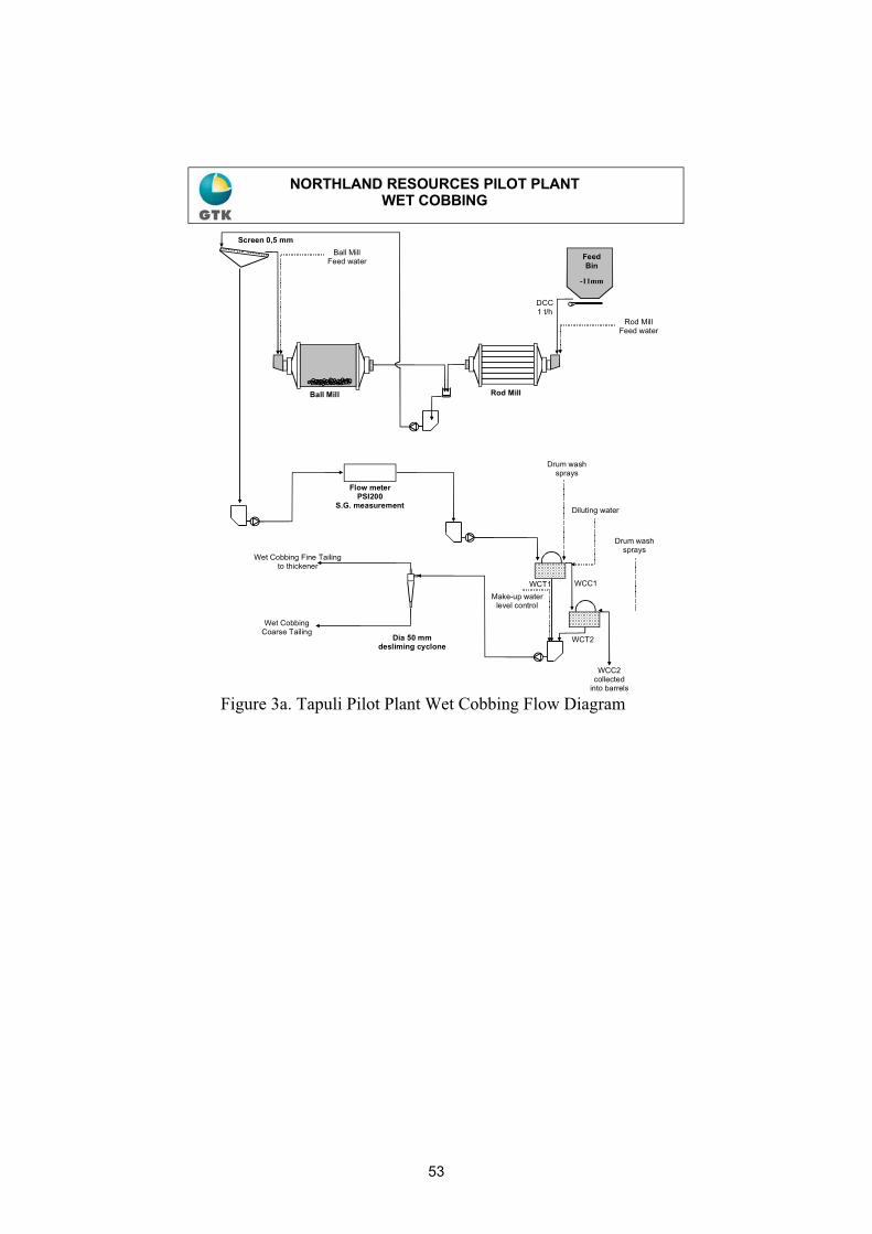
-11mm
FeedBin
Screen 0,5 mm
Wet Cobbing Fine Tailingto thickener
Wet Cobbing Coarse Tailing
NORTHLAND RESOURCES PILOT PLANTWET COBBING
Ball Mill Rod Mill
Flow meterPSI200
S.G. measurement
Rod MillFeed water
Ball MillFeed water
Make-up waterlevel control
Diluting water
Drum washsprays
Drum washsprays
DCC1 t/h
WCC2collected
into barrels
Dia 50 mmdesliming cyclone
WCC1WCT1
WCT2
Figure 3a. Tapuli Pilot Plant Wet Cobbing Flow Diagram
53

NORTHLAND RESOURCES PILOT PLANTWET LIMS SEPARATION 1
Flow meterPSI200
S.G. measurement
Make-up waterlevel control
Diluting water
Drum washsprays
Ball Mill
Drum washsprays
Drum washsprays
Diluting water
WLT1 WLT2
WLT3
WLC1
WLC2
WLC3 collectedinto barrels
WLT combined andpumped to thickener
Bredel typefeed pump
50 mmcyclone
Feed preparation conditioners
Mill Feedwater
Figure 3b. Tapuli Pilot Plant LIMS flow diagram
Figure 3. Tapuli Pilot Plant set-up of the wet cobbing (a) and wet LIMS (b) circuits.
Table 3. Tapuli Pilot Plant final concentrate assay.
Wt% Fet SiO2 Al2O3 CaO MgO S Na K Blaine(cm2/g)
TapuliConcentrate 69.3 0.95 0.14 0.10 1.99 0.045 0.007 0.013 1700
3.1.3 Further Developments
The pilot plant results will be used for basic engineering design of process plant and which will be incorporated into a prefeasibility study to be completed in early 2009.
Autogenous milling options may offer a substantial economic advantage and a different flowsheet will also be considered; however the metallurgical results of recovery and grade are not expected to change significantly.
54

3.2 Stora Sahavaara Flowsheet Development
Stora Sahavaara ore has been evaluated using numerous drill cores and from a 2200 tonne bulk sample taken in 2007. Significant bench scale characterisation and a full pilot plant have been conducted.
The testwork has been performed by SGS Lakefield and recently published.4 Stora Sahavaara ore, like that of Tapuli, is quite basic in nature, and requires the flotation of pyrrhotite at a low pH; which consequently involves significant acid consumption during the flotation stage of the process. The flowsheets under consideration are shown in Figure 4. It was noted in the work to date that the autogenous milling option was the lowest in overall energy consumption and produced the cleanest concentrate.
It was established early that in order to achieve a high quality Fe concentrate low in sulphur the Stora ore needed to be subjected to a fine grind (in order to liberate the sulphur) of at least a P80 of 90 microns and that flotation was needed to remove the magnetic pyrrhotite. Whilst the silica and alumina content of the concentrate produced from the bulk sample and pilot plant processing was low at <1.5% SiO2 + Al2O3, the MgO content was found to be quite high at >4%. Further grinding to around P80 of 40 microns (approximate to a pellet feed size) and additional LIMS separation improved the quality of the concentrate further by further lowering the MgO, SiO2 and Al2O3, and increasing the Fe content. The MgO content of the concentrate has under further investigation, described below.
55

Figure 4. Stora Sahavaara flowsheet options.
Variation testing revealed that the MgO content of the magnetite varies across the mineral resource, which prompted further evaluation of the resource using a series of Dings Davis tube tests on assay reject samples from a number of drill cores taken across the Stora resource to reflect early development of the mine.
The Stora Sahavaara mineral resource is comprised of a main lens, and an adjacent lens, “Södra Sahavaara”. In total 233 DDT tests have been performed on assay rejects (P85 of 75 micron) from circa 5 metre composite intervals from 18 drill holes in Stora Sahavaara including Södra Sahavaara lens. The locations are shown in Figure 5. In addition, EPMA-WDS Microprobe analysis was carried out on 37 samples of magnetic and non-magnetic fractions from DDT tests from 8 drill holes across.
56

The number of magnetite grains analysed for Stora Sahavaara (main lens) was 264. Based on these analyses the arithmetic and weighed average for the MgO content in magnetite is 2.12 % and 2.60% respectively. In the case of the Södra Sahavaara lens, 98 grains were analyzed showing significantly less MgO content, with arithmetic average of 0.33% and weighted average of 0.37%. The concentrates produced commercially will contain entrained or locked minerals such as serpentine. It should be expected that Stora Sahavaara concentrate will average between 2.7 and 3% MgO. The overall concentrate averages from Stora Sahavaara and Södra Sahavaara DDT tests are shown in Table 4. Note that the DDT tests were performed at a coarser particle size than the industrial case, and the concentrate still contains pyrrhotite.
Table 4. Dings Davis tube concentrate assays for samples from Stora Sahavaara and Södra Sahavaara. Notes: 1) no sulphide flotation was made, therefore the
concentrates include magnetic pyrrhotite which would be mostly removed in flotation; 2) the particle size was slightly coarser than in the anticipated industrial process giving poorer liberation in the DDT tests.
Satellite Av. mass-% Magnetics SiO2 TiO2 Al2O3 Fe MgO CaO Na2O K2O S
Stora Sahavaara 54,8 1,82 0,06 0,27 65,2 3,87 0,15 0,00 0,01 1,50Södra Sahavaara 36,6 1,67 0,07 0,17 67,5 1,46 0,28 0,01 0,02 0,44
3.2.1 Further Developments
A drilling program completed in 2008 has produced circa 25 tonnes of ore which provides a representative sample of the mineral resource. Further concentrate will be produced from this sample which will be better representative of the MgO content in the pellet feed concentrate from the early years of production from Stora Sahavaara and will provide an opportunity to better optimise the flowsheet.
57

Figure 5. Map of Stora Sahavaara including Södra Sahavaara lens (thinner zone toward the bottom of the map) showing drill holes with DDT tests (red dots). Drill holes with DDT samples subjected to EPMA-WDS shown with squares. The ore zone dips 50-70o west.
58

3.3 Hannukainen Flowsheet Development
From early metallurgical investigations of Hannukainen, it was determined that the best flowsheet for recovery of all minerals of interest, magnetite, copper and gold, required a flowsheet with the dry cobbing stage eliminated. This led to the conclusion that an AG/SAG option may be viable, or three stage conventional crushing. As previously reported4, there were three main flowsheet options for post-crushing beneficiation that were tested at bench scale. All involve flotation of pyrite, chalcopyrite, pyrrhotite and magnetic separation of magnetite in slightly differing configurations. Flowsheet 3, Figure 6, emerged as the best option with regard to recovery of iron, copper and gold. The chemical analyses of the streams derived from the bench scale work are shown in Table 5. Another flowsheet, Flowsheet 2, shown in Figure 7, was eliminated prior to optimisation due to anticipated high cost of pyrrhotite flotation if made prior to magnetic separation. However, this will be re-evaluated; as the loss of recoverable iron using Flowsheet 3 have been largely attributed to magnetite carryover in the pyrrhotite flotation. Magnetic entrainment of fine magnetite with pyrrhotite has been found, with an example shown in Figure 8. It may be possible to improve recovery using flowsheet 2 which places the flotation prior to the low intensity magnetic separation, or by adding a scavenger circuit after the pyrrhotite flotation. Re-evaluation of the flowsheet is also needed to establish the most economic approach, as flowsheet 3 requires all feed ore to be ground to <100 microns.
59

Grinding Circuit
1st Cleaner Scav
Final Fe Concentrate
Cu 3rd Cleaner Concentrate
1st Cleaner Scavenger Tail – Pyrite Conc
1
2
3
Product Legend
23
4
1st Cleaner
Chalcopyrite Rougher
3rd Cleaner
2nd Cleaner
M
5
1
Magnetic Separation Tail
Pyrrhotite Concentrate
4
5
LIMS
Pyrrhotite Rougher
Figure 6. Flowsheet 3 for processing Hannukainen ore.
Table 5. Flowsheet 3 Stream analyses from bench scale testwork.Element Unit Head Fe Conc Cu Conc Po Conc Py Conc Low S tailsCu % 0.26 0.002 26.2 0.15 0.33 0.012Fe % 35.2 70.6 31.8 63.3 39.7 8.53Au g/t 0.10 0.02 7.06 0.11 0.74 0.07S % 2.67 0.05 28.2 22.6 35.3 0.12SiO2 % 27.9 0.98 14.7 0.94 --- 49.3Al2O3 % 4.25 0.39 1.04 0.27 --- 6.83MgO % 4.42 0.35 0.60 0.24 --- 7.76CaO % 9.10 0.29 1.74 0.19 --- 16.1Na2O % 1.25 <0.01 0.21 0.02 --- 2.05K2O % 0.41 0.01 0.26 0.02 --- 0.76TiO2 % 0.19 0.11 0.06 0.05 --- 0.25P2O5 % 0.12 <0.01 <0.02 <0.01 --- 0.18MnO % 0.19 0.12 0.04 0.05 --- 0.27Cr2O3 % <0.01 0.02 0.003 0.05 --- 0.01V2O5 % 0.01 0.02 0.002 <0.01 --- <0.01LOI % 0.49 -2.97 14.0 8.04 --- 0.82Sum % 98.7 100.3 N/A 100.4 --- 99.0wt yield % 100 31.5 0.91 4.69 3.04 59.8
60

Grinding Circuit
1st Cleaner Scav
Final Fe Concentrate
Cu 3rd Cleaner Concentrate
1st Cleaner Scavenger Tail – Pyrite Conc
1
2
3
Product Legend
23
4
1st Cleaner
Cu Rougher
3rd Cleaner
2nd Cleaner
M
5
1
Magnetic Separation Tail
Pyrrhotite Concentrate
4
5
Py/Po RougherLIMS
Figure 7. Flowsheet 2 for processing Hannukainen ore.
Figure 8. Large pyrrhotite grain with a number of small magnetite grains – taken from pyrrhotite concentrate obtained from Flowsheet 3 testwork.
61

3.3.1 Further Developments
The resource has been evaluated in a preliminary geo-metallurgical program by SGS Mineral Services. A cluster analysis based on chemistry defining three different ‘clusters’ was made. Metallurgical response is planned to be tested for each of three ‘clusters’ as well as variability within the defined cluster, as well as retest the response for flowsheets 2 and 3 for each cluster at bench scale. This will be done using selected drill core from across the mineral resource.
In addition to the core being tested above, a further 12 tonnes of metallurgical core was drilled from across the resource, and 18 tonnes of ¼ core from exploration may be used for a mini-pilot plant in order to confirm the final flowsheet and produce concentrates for product development.
4. Conclusions
Flowsheet options have been developed for processing of Tapuli, Stora Sahavaara and Hannukainen ore. All three ores require relatively fine grinding, to less than 100 micron in order to produce high grade magnetite concentrate. Autogenous grinding alternatives in lieu of conventional 3-stage crushing and ball milling will be considered for all three flowsheets. All three resources can produce high quality (low silica plus alumina) iron ore concentrates suitable for pelletising.
Hannukainen and Stora Sahavaara ores require flotation to remove pyrrhotite. While pyrrhotite flotation at low pH has shown to be successful, further testwork at near neutral pH will be undertaken. Further testing of variability of metallurgical response is underway for Hannukainen.
Work has started on a pre-feasibility study and revised preliminary economic evaluations of the Swedish Resources, along with additional exploration and characterisation of selected targets in the Pajala and Kolari regions as well as NI43-101 compliant resource estimates anticipated during 2009 for Pellivuoma and Kuervitikko.
5. Acknowledgements
The authors wish to thank Mr. Tapio Knuutinen, Mr. Markku Kuusisto, Mr. Markku Klemetti and Mr. Pekka Mörsky and their colleagues at the Geological Survey of Finland for their work on the Tapuli pilot plant; and Mr. André McKen, Ms. Dominique Lascelles, Mr. Guillaume Chiasson, Dr. Guillermo Turner-Saad and Dr. Christian Dragusanu and their colleagues at SGS Mineral Services, Lakefield, for their work on the Hannukainen and Stora Sahavaara flowsheet development.
The assistance of Mr. Esko Pöyliö and Dr. Kyösti Heinänen is gratefully acknowledged.
62

6. References
1. Mukhopadhyay, D.K., Steedman, J., Lindholm, T. ”Mineral Resource Estimates for the Hannukainen Deposits, Kolari Area, Finland”, NI43-101 Technical Report, Micon International Co Limited, 2007.
2. Barry, J.P.; Sandefur, R.L., “Technical report, Stora Sahavaara Project, Northern Sweden”, Chlumsky, Armbrust & Meyer LLC, 2006.
3. News release, “Northland Upgrades Resource Figures for Tapuli Magnetite Project”, Northland Resources Inc., December 11, 2008.
Note: NI43-101 report release pending.
4. Lascelles, D., McKen, A., Chiasson, G., Marsden, P., Hooey, L., Dixon, A., Houseley, K., ”The recovery of metals from the Stora Sahavaara and Hannukainen Iron Oxide Copper Gold (IOCG) Resources”, Procemin 2008, Oct. 22-24, 2008, Santiago, Chile, pp. 229-240.
5. Lindholm, T., Mukhopadhyay, D.K., Steedman, J.,”Tapuli Resource Estimate”, GeoVista AB, 2008.
63

64

Treatment of process water from molybdenum flotationIkumapayi Fatai K1, Jan-Eric Sundkvist2 and Nils-Johan Bolin3
1Division of Mineral Processing and Metallurgy, Luleå University of Technology, SE-971 87 Luleå, Sweden, [email protected]
2&3Division of Process Technology, Boliden Mineral AB, SE-936 81 Boliden, Sweden, [email protected],[email protected]
AbstractThe Boliden copper mine in Aitik, north of Sweden is aiming to produce molybdenum as a new product. Due to the use of sodium hydrogen sulphide (NaHS) as a depressant of copper concentrate during the molybdenum flotation, it was a concern that the tailings pond cannot buffer the potential acid generation when free hydrogen sulphide ions (HS-) and degradation products such as thiosulphate ions (S2O3
2-) are further oxidized downstream to sulphate ions (SO4
2-). There was also a concern regarding possible dissolution of heavy metals into the process water, for example mercury. Test work carried out aiming to generate data for the design of a suitable process for treatment of the process water before discharging it from the molybdenum flotation circuit into the tailings pond, demonstrates that: A significant portion of the Chemical Oxygen Demand (COD) can be removed by aeration of the pulp through oxidation of HS- and polysulphides to elemental sulphur and thiosulphate. Subsequent flocculation test work on the oxidised pulp has shown that elemental sulphur as well as precipitated mercury or fine mercury minerals will go to the final copper concentrate by sedimentation. The thiosulphate content in the overflow from the solid-liquid separation of the oxidised pulp can be completely converted to sulphate using hydrogen peroxide based on the Fenton procedure. The overflow was finally neutralized using slaked lime. Acceptable water quality to the tailings pond could be accomplished.
Keywords: NaHS; conditioning; COD; flotation; thiosulphates; aeration; Fenton oxidation
1 Introduction The predominant process employed to produce molybdenite from copper concentrate is to depress copper sulphides, capitalizing on the surface property of the easy floatability of molybdenite. The depressant agent commonly used is sodium hydrogen sulphide (NaHS). Addition of NaHS reagent to the pulp reduces the redox potential to a level where copper sulphides are un-floatable. Depression of copper sulphide starts at a Redox potential of about -250 mV. However, for an efficient depression, the Redox potential is maintained between -450 and -500 mV. The reaction mechanism is not completely understood, however, the addition of NaHS allows for obtaining sulphides with a fresh surface because it desorbs the collector, making depression easy (Equation 1-1; X signifies the collector). The surface of chalcopyrite is also modified from hydrophobic to hydrophilic (Equation 1-2) and there is high possibility of elemental sulphur desorption from the surface of the concentrates (Equation 1-3) (Ikumapayi, 2008).
2CuX(s) + HS- Cu2S(s) + 2X- + H+ (1-1)2CuFeS2 + HS- S2
2- + H+ +Cu2S(s) + 2FeS(s) (1-2)So + HS- S2
2- + H+ (1-3) The proposed addition rate of NaHS at Aitik is in the range of 5-8 kg per tonne of copper concentrate and it was a concern that the tailings pond cannot buffer the potential acid generation when free HS- and degradation products, mainly thiosalts, are further oxidized downstream to SO4
2-
(Equations 1-4 and 1-5) (McGeer et al., 2000 and Schwartz et al., 2006). HS- + 2O2 SO4
2- + H+ (1-4) H2O + S2O3
2- + 2 O2 2 SO42- + 2 H+ (1-5)
65

At the nominal production rate of 343000 ton of copper concentrate, the expected addition of NaHS has a potential to produce 950-1500 ton of sulphuric acid per year. Another concern is possible dissolution of heavy metals into the process water (Bolin and Jönsson, 2007). For example mercury and antimony sulphides can dissolve in alkaline sulphide solution by forming stable metal-sulphide complexes. Table 1 is a thermodynamic calculations result of Hg-sulphide-water system based on an algorithm described by Eriksson (Ericsson, 1979). As can be seen from the results, the solubility of Hg is significant and depends strongly on pH at the expected NaHS concentration in process solution.
Table 1: Calculated equilibrium concentrations of mercury species at 5.85 kg/m3 NaHS in solution Calculated equilibrium concentrations of Hg2+ species
Solubility Hg2+ Hg(HS)2(aq) HgS22-(aq) HgS(s)
pH mg Hg/l log([x]/M) log([x]/M) log([x]/M) log([x]/M) 13.00 576.7 -51.06 -12.74 -2.54 -2.1512.75 418.7 -50.92 -12.38 -2.68 -2.1012.50 281.6 -50.75 -12.05 -2.85 -2.0712.25 177.9 -50.55 -11.75 -3.05 -2.0412.00 107.5 -50.33 -11.47 -3.27 -2.0211.75 63.1 -50.10 -11.20 -3.50 -2.0111.50 36.4 -49.86 -10.94 -3.74 -2.0111.25 20.8 -49.61 -10.69 -3.99 -2.0011.00 11.8 -49.37 -10.43 -4.23 -2.00
Mo flotation w
orking range
2 Literature review A number of attempts have been made to remove thiosalts from mining effluents, most of which are either site/effluent specific, uneconomical or ineffective (Wasserlauf and Dutrizac, 1982 CANMET, 1998 Dinardo and Salley, 1998 Li and Boucher, 1999 Riveros and Chaulk, 2000 Sridhar, 2001 Gould et al., 2004): Co-precipitation with ferric salts as well as natural degradation in which the thiosalts concentration is expected to be oxidised naturally by dissolved oxygen in the effluents was ineffective due to factors such as temperature, nutrients, oxygen concentration and bacterial populations in the effluents (Riveros and Chaulk, 2000 and Gould et al., 2004). Direct photolytic process (DPP), which involves the destruction of thiosalts by direct absorption of ultraviolet (UV) irradiation by the thiosalts and their progeny, and subsequent chemical interactions in the aqueous phase was effective but uneconomical (Sridhar, 2001). SO2/air oxidation process in the presence of iron is a viable process for thiosalt destruction but site/effluent specific, each effluent has to be characterized individually in order to identify the catalysts/elements present in solution and their effect on the oxidation kinetics (CANMET, 1998). Chlorination, ozonation, hydrogen peroxide, chalcopyrite catalysis, alkaline pressure oxidation, bicarbonate addition and reduction by iron achieved complete thiosalts removal, and almost complete removal in the case of biological oxidation; these methods are technically feasible however there is a high degree of uncertainty regarding the effectiveness of these technologies to treat large volumes of effluent on a continuous basis (Dinardo and Salley, 1998 Li and Boucher, 1999).
3 Test work description 3.1 GeneralThe test work procedures have been developed on an ongoing basis since no standard methods for destruction of thiosalts in process water from a molybdenum circuit are available or known.The conducted test work will be presented in a chronological order.
66

3.1.1 MaterialThe copper and pyrite concentrates used as feed were obtained fresh at the Boliden concentrator in Aitik, Sweden. Technical grade NaHS flakes (~70% NaHS) were used as depressant of copper sulphide. Nitrogen gas was used to create inert atmosphere when necessary. The flocculant used is known as Magnafloc 351, hydrogen peroxide, (H2O2, 35%) was used as oxidising agent, ferrous sulphate pentahydrate, (FeSO4 .7 H2O, green vitriol or melanterite) was used as catalyst during effluent oxidation, technical grade sodium hydroxide, (NaOH), sulphuric acid, (H2SO4) and slaked lime, (Ca(OH)2) were used as pH regulators. All chemicals and reagents were collected from Concentrator’s laboratory in Boliden. 3.1.2 Analytical methods The COD reflects the maximum oxygen uptake requirement of the process water. It is measured with the aid of Hach-Lange spectrophotometer DR 2800 (oxidizable substances present in the water sample react with sulphuric acid-potassium dichromate solution in the presence of silver sulphate as a catalyst, potassium dichromate is reduced forming Cr3+. The amount of green coloration of Cr3+ is evaluated in the spectrophotometer and is used as an indirect measure of the oxidizable contents of the water sample (Clair et al., 2003). The elemental sulphur, (So) and tetrathionate, (S4O6
2-)concentrations were determined by cyanolysis followed by spectrophotometric determination of formed thiocyanate (SCN-) (Mizoguchi and Okabe, 1975). Thiosulphate, (S2O3
2-) and sulphite, (SO3
2-) concentration were analyzed by iodometric titration (Koh, 1990). The sulphate, (SO42-)
concentration was analyzed by spectrophotometric turbidity measurement of precipitated barium sulphate (BaSO4) (Meneses et al., 2005). The sulphide, (HS-) concentration in solution was analyzed by calculation from COD difference before and after eliminating sulphide as H2S from the solution by blowing nitrogen through the solution. The ammonia/ammonium concentration in the final solution from the testwork with ammonium sulphide conditioning was determined by the Hach/Lange method. An attempt to detect any desorbed xanthate present in the solution was done by addition of copper (II) sulphate and Cu(I)-chloride. The presence of xanthates is indicated by precipitation of yellow copper xanthate. The dissolved oxygen in the pulp and solutions was measured by inserting the probe of a Hach-HQ 30d flexi oxygen meter directly into the pulp or solution. The Redox potential was measured against Ag, AgCl reference electrode with the aid of an Orion 230A+ Redox meter. The pH was measured with the aid of an Orion 210A pH meter.
3.2 Test series no. 1: simulating natural degradation of process water Test series no. 1 was based on a concept where most of the process water is recycled, see Figure 1. Bleed from the copper concentrate thickener overflow is diverted to the planned pyrite tailings pond, where oxidizable components in the water are naturally degraded by the action of air. pH and metals in the discharged water from the pyrite pond can be controlled by further treatment with lime addition.
67

C o p p e r c o n c e n tra te w ith M o f ro m C u /p y r ite s e p a ra t io n c irc u it
T h ic k e n e r
6 5 % s o lid s
O v e r f lo w
F in a l c o p p e r c o n cth ic k e n e r
P re -c o n d itio n e rN a H S
s to c k ta n k
4 5 % s o lid s
M o -C u s e p a ra t io nf lo ta t io n c irc u it
F in a l c o p p e r c o n cf ilt ra t io n
O v e rf lo w
F in a l M o c o n cth ic k e n e r
F in a l M o lly - c o n cf ilt ra tio n
O v e r f lo w
M a k e -u p w a te r
T o s m e lte r
T o s m e lte r
F ilt ra te
F ilt ra te
6 5 % s o lid s
A ir o r N 2 o r re c yc le d a ir a s f lo ta t io n g a s
P ro c e s s w a te r b le e d to th e p y r ite ta ilin g s p o n d
P yr ite c o n c e n tra te
Figure 1: Conceptual flow sheet no. 1: Natural degradation of process water bleed
About 2 kg of Aitik copper concentrate was pulped and agitated at about 45 % solids in reactors provided with water jackets. The condition/flotation simulation was carried out at two temperatures, 5 and 18 oC, respectively which are assumed to cover the expected operational temperature range. NaHS was added to the pulp initially to obtain a Redox potential of about –530 mV followed by 10 minutes conditioning. Air was then introduced under the impeller to simulate the flotation for 30 minutes. Redox of about –570 mV was maintained with addition of more NaHS. After flotation, the pulp was allowed to settle overnight and the overflow was filtered for the subsequent oxidation test work. The filtered overflow was split and transferred to 3-litres glass vessels provided with agitators. The vessels were submersed in a water bath provided with a temperature-controlled dip-cooler. The solutions were oxidized by the action of air by vortex formation and oxygen uptake only by gentle agitation. The test work performances are summarized in Table 2.
Table 2: Test work performance summary, test series no. 1
Flotation conditions Thickener O/F treatment Test Temp ConditioningAeration Redox targetThickening Type of aeration Temp no. oC minutes minutes mV hours Intensity oC1:a 5 10 30 -530/-570 17 Gentle agitation, no vortex formation 51:b 5 10 30 -530/-570 17 Forced agitation, vortex formation 51:c 18 10 30 -530/-570 17 Gentle agitation, no vortex formation 51:d 18 10 30 -530/-570 17 Forced agitation, vortex formation 5
3.3 Test series no. 2: Effect of pyrite in NaHS solution The aim of test series no. 2 was to investigate the effect of the presence of pyrite during prolonged aeration of a synthetic NaHS-solution in order to simulate the possible chemical reactions in the planned pyrite tailings pond. The aeration was done in a bioreactor where air was introduced under the impeller. The test work performances are summarized in Table 3.
Table 3: Test work performance summary, test series no. 2 Test Temp NaHS concentrationPulp density no. oC g/l % solids 2:a Ambient 4.3 02:b Ambient 4.3 43
68

3.4 Test series no. 3: Mode of thiosalts and heavy metals formation The aim of test series no. 3 was to simulate the process conditions by following the formation of thiosalts and dissolution of heavy metals (specifically mercury) in the process water. An additional aim was to verify possible precipitation of heavy metals as metal-sulphides back into the concentrate by extensive oxidation of the pulp, thereby reducing free HS- and polysulphides concentration in the solution. Tests were carried out at both low (5 oC) and ambient (16 oC)temperatures in order to simulate (extreme) cold as well as warmer conditions. Pulp of 35% solids was conditioned with 4 to 633 kg NaHS/tonne concentrate in a 3-liter closed glass reactor, in a nitrogen atmosphere. The pH was maintained at approximately 11(with addition of sodium hydroxide solution when required), conditioning lasted for 30 - 83 minutes in order to achieve a better depression of copper at Redox potential of approximately -500 mV. Both dried stored and wet fresh copper concentrates were used in the tests. Aeration was carried out extensively for 4 to 5 hours by introducing air or oxygen into the pulp with agitation by stirring. The test work performances are summarized in Table 4.
Table 4: Test work performance summary, test series no. 3 Test Temp Conditioning Aeration Aeration gas Material NaHS no. oC minutes hours kg/t3:a 16 60 5 O2 Dry stored Cu conc. 293:b 5 30 5 O2 Dry stored Cu conc. 113:c 16 30 4 O2 Fresh wet Cu conc. 4.3 3:d 16 30 4 Air Fresh wet Cu conc. 4.3 3:e 16 83 5 O2 Dry stored Cu conc. 633 3:f 16 30 4 Air Fresh wet Cu conc. 4.3 3:g 16 30 4 Air Fresh wet Cu conc. 4.3
3.5 Test series no. 4: Treatment of the process water Test series no. 4 is a number of flotation-oxidation test works based on a concept where the sulphur species are removed from the solution step wisely see Figure 2. The tests were carried out in a lab scale flotation cell, in order to simulate real process conditions, including conditioning, flotation, subsequent oxidation of the pulp, solid liquid separation as well as oxidation and neutralization of final solution. The formation and destruction of thiosalts in solution was followed throughout the experiment. A 3-liter WEMCO flotation cell was used throughout the experiment. During the low temperature experiment, the cell was placed in a water bath, which is cooled with the aid of a cooling bar. Pulp of fresh copper concentrate, 30% solids was conditioned with 8 kg NaHS/tonne concentrate for approximately 10 minutes in a nitrogen atmosphere. The pH was maintained at approximately 11, using sodium hydroxide. A single test was carried out in which the pulp was initially conditioned for 24 hours using ammonium sulphide. Flotation was carried out for approximately 30 minutes after conditioning using nitrogen gas. The remaining pulp was oxidized with air or oxygen until a tendency of unmanageable foaming was observed.
69

C opper concentra te w ith M o from C u/pyrite sepa ra tion c ircu it
T h ick ener
65 % so lids
O ve rflow
F ina l coppe r concth ick ener
P re-cond ition ingN aH S
s tock tank
45% so lids
M o-C u sepa ra tionflo ta tion c ircu it
F ina l coppe r concfiltra tion
O ve rflow
F ina l M o - concth ick ener
F ina l M o - concfiltra tion
O verflowM ake -up fresh w ater
T o sm elte r
T o sm elte r
F iltra te
F iltra te
65 % so lids
A ir o r N 2 o r recyc led a ir as f lo ta tion gas
P rocess w a ter b leed to the pyrite ta ilings pond
P yrite concentra te
P u lp ox ida tion
N 2
A ir o r O 2
P u lp po lish ingby pe rox ide
H 2O 2
F loccu lan t
P e rox ide ox ida tion by F en ton p rocedure
N eu tra liza tion by lim e add ition
Figure 2: Proposed flow sheet no. 2
Aeration was carried out at high (11 to 12) and low (7 to 8) pH as well as ambient (16 to 19 oC) and low (5 to 7 oC) temperatures. The final pulp was further oxidized by addition of hydrogen peroxide when pulp-oxidation was carried out at high pH, in order to completely remove the polysulphides and thereby ensuring the precipitation of heavy metals. The end-point was indicated by the disappearance of the yellow coloration of the solution and smell of H2S. A solution of 0.92-g/l Magnafloc 351 was subsequently added to the pulp in order to speed up the settling rate and obtain a clear overflow. The solution was decanted and analyzed for dissolved species.
3.5.1 Final oxidation by means of Fenton procedure The clear solution was analysed for thiosalts concentration via COD and iodometric titration for calculation of the stoichiometric H2O2 demand to subsequently oxidize the thiosalt content completely to sulphate based on Fenton’s reagent procedure (Fenton’s reference). The Fenton testwork was carried out batchwise. The pH of the solution was controlled between 3.5 and 5. Iron II catalyst was added as a solution of FeSO4 to a concentration of approximately 60 mg Fe/l and the H2O2 solution was added slowly, while the pH was maintained within the above-mentioned range. Faster addition rates of the H2O2 solution inhibit the catalyst (Fenton’s reference). The acidic solution was finally neutralized to approximately pH 9 by addition of powdered slaked lime, Ca(OH)2. The variable factors in performed test work are summarized in Table 5.
Table 5: Variable factors summary in test series no. 4.
Test Temp
no. oC hours kg/t pH Gas4:a 16 - - Natural Air and O2
4:b 16 - - Natural Air4:c 16 - - Natural Air4:d 16 - - 7.5-8.5 Air4:e 16 24 1.7 7.5-8.5 Air4:f 16 - - 7.5-8.5 Air4:g 16 - - 7.5-8.5 Air and N2
4:h 5 - - 7.5-8.5 Air4:i 16 - - 7.5-8.5 Air4:j 5 - - Natural Air4:k 5 - - Natural Air4:l 5 - - 7.5-8.5 Air
(NH4)2S conditioning Pulp oxidation
Note: Natural pH is about 11.
70

4 Results4.1 Test series no. 1 The assay results from sampling of the solutions from simulated flotation tests are summarized in Table 6. Table 6: Solution chemistry results from test work series no.1
Ag Bi Sb Hg SiO2 Redox*
Test solutions mg/l mg/l mg/l mg/l mg/l pH mV Solution Test 1 a, b; 10 minutes conditioningc <0.1 0.77 1.1 5.7 12.6 11.2 -539 Solution Test 1 a, b; 30 minutes aeration <0.1 0.8 5.3 4.49 11.9 -567 Solution Test 1 a, b; 17 hours settling 12.2 -497
Solution Test 1 c, d; 10 minutes conditioning <0.1 2.1 8.2 27.2 11.7 -533 Solution Test 1 c, d; 30 minutes aeration <0.1 1.2 8.4 17.2 12.1 -571 Solution Test 1 c, d; 17 hours settling 12.2 -413 * vs. Ag, AgCl reference electrode As can be seen in Table 6, considerable concentrations of Hg, Sb and Bi were found in the filtered process solutions. It can also be noticed that the pH of the solutions increased during the course of aeration. Figures 3-4, shows the profiles obtained from the subsequent prolonged aeration of the filtered process solutions.
Figure 3: (Top left and right): pH and Redox profiles test 1a and 1b respectively (Bottom left and right): Sulphur species profiles test 1a and 1b respectively
71

Figure 4: (Top left and right): pH and Redox profiles test 1c and 1d respectively (Bottom left and right): Sulphur species profiles test 1c and 1d respectively
Figure 5 shows the obtained milky solutions containing colloidal sulphur and polysulphides.
Figure 5: Prolonged aeration test work setup showing the formation of colloidal sulphur
The results show that natural oxidation of the overflow is most probably a very slow and incomplete process. The final solution contained mainly thiosulphate, colloidal sulphur and polysulphides after two weeks of continuous oxidation and it is anticipated that neutralization would be very difficult to control at the existing tailings pond in Aitik however, the solution has potential to be completely oxidized to sulphuric acid, and there is also a risk of uncontrolled discharge of dissolved heavy metals such as mercury into the pond. Therefore a different process route was considered in test series no. 3 and 4.
72

4.2 Test series no. 2 The results from the sampling of the solution and pulp are shown in figure 6
Figure 6: Test 2a, 2b (Top left): pH and Redox versus aeration time (Top right): Chemical oxygen demand versus aeration time (Bottom left): Thiosulphate concentration defined by I2 titration versus aeration timeFigure 6 shows that presence of pyrite surfaces increase the initial COD and sulphur species removal rate. However, there seems not to be any significant improvement of the final results. The apparent very high concentration of thiosulphate indicated in the beginning is due to co-titration of HS- and polysulphides. The iodine titration indicates about the same concentration of reduced sulphur species in the final solution. Final COD is somewhat higher for pyrite pulp, which may be explained by the presence of fine solids in the filtrate. The abnormal thiosulphate profile between day 1 and 5 for the pyritic pulp cannot be easily explained and is most probably an analytical anomaly. 4.3 Test series no. 3 The assay results from sampling of the solutions and solid residues are summarized in Table 7. Table 7: Assay results, final conditions from test series no.3
Test Temp Aeration gas NaHS
Assayed head
Hg in residue
Hg in final solution
Calc.Head Redox range
no. oC kg/t g Hg/t g/t µg/l g Hg/t mV 3:a 16 O2 29 43.1 28.1 0.83 28.1 -629 to -10 3:b 5 O2 11 43.1 39.6 0.23 39.6 -603 to -17 3:c 16 O2 4.3 23.5 29.2 3.59 29.2 -496 to -17 3:d 16 Air 4.3 23.5 24.7 0.61 24.7 -496 to 15 3:e 16 O2 633 43.1 17.8 6060 27.4 -506 to -683 3:f 16 Air 4.3 23.5 30.2 7-15 30.3 -482 to 0.3 3:g 16 Air 4.3 23.5 N/A 2.5-6 N/A -368 to 13.7
The calculated and assayed head (mercury grade in the concentrate) of mercury concentration was in good agreement only in tests 3:b and 3:d while it is not balance in the remaining tests. The unbalanced situation could not be easily explained. It appears that the deviation is more significant at high mercury grade, tests 3:a and 3:e than at lower grade, except when the conditioning was carried out at low temperature, test 3:b. This may indicate that the actual found concentration of
73

mercury in the final solution is underestimated in the solution from the ambient temperature tests. At low temperature it can be expected that the dissolution of mercury is slow and more incomplete compared to higher temperatures. Losses of colloidal or very fine particles of mercury to the filtrate may also explain the deviation between calculated head and direct assayed heads. The degree of dissolution of mercury may also depend on mineralogy of the ore. The mercury may occur as HgS or as amalgam together with precious metals, AuAgHg. The mineralogy and grade may vary in the concentrate depending on actual ore treated in the concentrator. In Table 8, the Hg profile in solution is summarized, for non-filtered (decanted after settling) and filtered solutions, respectively. This was done in order to establish any effect of suspended solids on the solution assays.
Table 8: Test 3f Mercury profile, non-filtered and filtered solution Hg in solution µg/l Process stages Non-filtered Filtered
Feed, without NaHS 6.9 3.66 Feed, with NaHS 665 4.59 30 minutes conditioning 523 4.73 30 minutes aeration 146 0.49 1 hours aeration 8.26 0.16 2 hours aeration 9.11 0.05 2.5 hours aeration 218 0.60 3 hours aeration 14.3 0.80 3.5 hours aeration 77.6 7.07 4 hours aeration 6.91 14.9
Table 8 shows that high mercury concentrations are more frequent in non-filtered solutions. This indicated that the mercury is enriched in the fine fractions of the copper concentrate. However, at some of the sampling points, the assayed concentration of mercury was higher in the filtered solution. This could either be due to analytical errors or uncontrolled losses by precipitation of mercury during sample storage. In addition, the Hg concentration in the final solution is in general approximately the same as that found in the pulp solution before NaHS was added. It was also observed that the solution was yellow even after 4 hours, indicating presence of residual polysulphides (S2
2-). The indicated presence of mercury in the intermediate solution may be due to low concentration of free S2-, which stabilizes the soluble HgS2
2- complex. The increase of mercury in the solution during aeration may be explained by the nature of mercury mineralogy. For example elemental mercury requires an oxidant for dissolution. Such oxidant might be the formed polysulphides. See equation 4-1. Hgo + S2
2- HgS22- (4-1)
Therefore, to control the discharge of mercury to the pond, the concentration of suspended solids in the process bleed solution has to be minimized by flocculation or coagulation after complete oxidation of the pulp. By this procedure any fine particles composed of mercury, elemental sulphur and other constituents will go to the final copper concentrate.
4.4 Test series no. 4 A sequence of COD concentration from flotation-oxidation tests sampled solutions is summarized in Figure 7. Figure 7 shows available results of analyzed COD concentrations present in the solution at each stage of the test work carried out at different test conditions as shown in the legend. Full data of each test stage are not available in all the experiment due to laboratory circumstances and aim of each experiment.
74

Figure 7: Solution COD concentrations at different test stages
The most probable main chemical reactions at different process stages are outlined as follows: Initial mixing with NaHSReaction with dissolved oxygen in the process water: 2HS- + 2 O2 S2O3
2- + H2O (4-2)
Conditioning with NaHSThe following reactions give a COD net increase and consume alkali: Dissolution of elemental sulphur: HS- + So H+ + S2
2- (4-3) Collector desorption: 2 CuX + HS- Cu2S + 2 X- + H+ (4-4) (1 mmol of HS- gives about 64 mg COD, while 1 mmol of amyl xanthate gives 312 mg COD as per measurement)
Elemental sulphur may also be disproportionated by the action of the high alkalinity: 4 So + 4 OH- 2 HS- + S2O3
2- + H2O (4-5)
The following reaction gives a COD decrease contribution: Sulphidation of metal hydroxides: HS- + Me(OH)2 MeS + H2O + OH- (4-6)
Minor air introduction to pulp may also contribute to COD decrease: 2HS- + 2 O2 S2O3
2- + H2O (4-7) HS- + 2 O2 SO4
2- + H+ (4-8)2HS- + 0.5 O2 S2
2- + H2O (4-9)
75

The observed net increase of COD as well as the slight decrease of pH during conditioning indicates that COD generating reactions are dominating. Analysis of the feed concentrate shows that it contains about 0.4% So and the indicated So concentration in the solution was estimated to corresponds to about 7.9 % of the sulphur from the concentrate.
N2 flotation During flotation with nitrogen it can be anticipated that the same type of reactions occur as during conditioning. However, it was observed during testwork that only minor changes of pH, redox and COD occurred during flotation provided that introduction of air was minimised. Possible anaerobic reactions seem to go to the end already during conditioning.
AerationpH increase was observed during the pulp aeration. The analyses of the solution during aeration indicate that the following reactions may occur: 2HS- + 2O2 S2O3
2- + H2O (4-10) 2HS- + 0.5O2 S2
2- + H2O (4-11) S2
2- + H2O + 0.5 O2 2So + 2OH- (probable cause of pH increase) (4-12) S2
2- + H2O HS- + So + OH- (4-13) HS- + 2O2 H+ + SO4
2- (4-14)
The formation of more So will diminish the concentration of HS- and S2- in solution. When the concentration of free HS- and S2- became very low; any dissolved mercury will precipitate: HgS2
2- + H2O HgS(s) + OH- + HS-(further oxidised) (4-15)
H2O2 oxidationPeroxide was used as oxidant both as a pulp polisher and in the subsequent solution oxidation stage: The following reaction may describe the polishing stage, which is carried out without pH control: H2O2 0.5O2 + H2O (4-16) 2HS- + 4H2O2 S2O3
2- + 5H2O (4-17) 2HS- + 2O2 S2O3
2- + H2O (4-18) S2
2- + H2O2 2So + 2OH- (4-19) HS- + 4H2O2 H+ + SO4
2- + 4H2O (4-20) S2
2- + H2O HS- + So + OH- (4-21) 3H2O2 + So SO4
2- + 2H+ + 2H2O (4-22)
The solution from the pulp polishing stage mainly contains thiosulphate, which is further oxidised completely to sulphate by means of the Fenton procedure. The following equation describes the overall reaction: S2O3
2- + 4H2O2 2SO42- + 2H+ + 3H2O (4-23)
Iron (II) sulphate is used as a catalyst in the Fenton procedure in order to generate reactive hydroxyl radicals for stochiometric usage of added peroxide (Michael et al.,2003 Fenton’s reference).
Fe2+ + H2O2 Fe3+ + OH- + .OH (4-24)
Fe3+ + H2O2 Fe2+ +.OOH + H+ (4-25)
76

Recycling of NaHSFree sulphide and sulphide occurring as polysulphides in the solution can be recovered or stripped by acidification with e.g. sulphuric acid (Equations 4-26 and 4-27) followed by scrubbing of the stripped H2S with a caustic soda solution which produces NaHS (Equation 4-28). StrippingH+
aq + HS-aq H2Sg (4-26)
2H+aq + S2
2-aq H2Sg + So
s (4-27)
ScrubbingNaOHaq + H2Sg NaHSaq + H2O (4-28)
Table 9 shows a summary of result of process interest.
Table 9: Summary of important test results: Approximate reagent consumption and final COD
Pulp oxidation by air Polishing H2S stripping Settling Fenton Overall
Total O2 uptake H2O2 H2SO4 Magnafloc g/t H2O2 H2O2 COD mg/l S2O32-
mg/l kg/t kg/t g/t kg/t kg/t mg/l mg/lAmbient temperature, low pH 42 3,24 40 2,29 2,29 38,8 0Ambient temperature, high pH 134 0,905 50 5,20 6,11 69,2 0Low temperature, low pH 5,05 40 1,64 1,64 66,6 0Low temperature, high pH 46 0,835 3,27 4,10 345 72,8
Final assayProcess stages
Experiment
5 Conclusion1. The testwork has shown that oxidation of a clear bleed solution from the molybdenum flotation
circuit is a very slow process ending up with colloidal sulphur and thiosulphates. 2. The testwork has shown that in-situ oxidation of the process solution is the preferred route. 3. The thiosulphate content in the overflow from the solid-liquid separation of the oxidised pulp
was completely converted to sulphate by hydrogen peroxide based on Fenton procedure, which was finally neutralized using slaked lime.
4. Flocculation of oxidised pulp has shown that elemental sulphur and precipitated mercury or fine mercury minerals will go to the final copper concentrate by sedimentation. This will ensure acceptable quality of the bleed water to the tailings pond.
5. Elemental sulphur present on the surface of the concentrate is dissolved by NaHS forming polysulphides, which gives rise to an increase in COD during conditioning.
6. The testwork has also indicated a possible route for recycling of a significant portion of added NaHS by performing the aeration at a pH controlled between 7 and 8.5 with addition of sulphuric acid.
7. The oxidation testwork carried out at low temperature, 5-8 oC, shows that oxidation rate decrease significantly at high pH. In spite of 4 time’s longer aeration time, the residual COD level was higher compared to aeration at 16 oC or aeration at low pH.
8. No residual xanthate was detected in the treated process water. It was not confirmed if degradation species from xanthate like carbon disulphide is present in the treated process water.
6 Acknowledgement We express our profound gratitude to the management of Boliden Mineral AB for granting us permission to publish information on this project.
77

7 References Bolin Nils Johan, Jönsson Hans (2007) Expansion from 18 to 36 Mton at the Aitik concentrator.New Boliden internal report CANMET (1998) An evaluation of SO
2/air mixture for thiosalts destruction from metal mining, Progress Report No. 1,
1998 Clair N. Sawyer, Perry L. McCarty, Gene F. Parkin (2003) Chemistry for Environmental Engineering and Science 5th ed.).pages 626-629 New York: McGraw-Hill. ISBN 0-07-248066-1.Dinardo O., Salley J (1998) Treatment of thiosalts in milling effluents: A review of treatment processes CANMET- MMSL Report 97-060(CR) Eriksson, G (1979) Anal. Chim. Acta, 112, 375-83 Gould W.D., Kawaja J., Bédard P., Dinardo O and Morin K (2004) Characterization of natural degradation of thiosalts within a tailings pond, CANMET- MMSL Report 04-002(CR) Ikumapayi F.K (2008) Purification of molybdenite concentrates. Masters thesis Luleå University of Technology. ISSN 1653-0187/ ISRN LTU-PB-EX--08/012--SE / NR 2008:012 Koh Tomozo (1990) Analytical chemistry of polythionates and thiosulfate. Analytical Sciences Vol.6 Li M, Boucher J.F (1999) Thiosalts treatment by bicarbonate addition, The thiosalt consortium, Noranda Inc., Technology Centre Environment Program Contract number 23440-8-1003/001/SQ McGeer James C, King Morgan, Brigham Sarah, Nadeau Jennifer (2000) The Acute toxicity of Sulfur Oxyanions to
Daphnia magna and Selenastrum capricornutum, CANMET-MMSL Project No. 602065 Meneses Silvia R.P, Maniasso Nelson, Zagatto Elias A.G (2005) Spectrophotometric flow-injection determination of sulphate in soil solutions. Talanta 65 1313–1317 Michael J. Borda, Alicia R. Elsetinow, Daniel R. Strongin, Martin A. Schoonen (2003). A mechanism for the production of hydroxyl radical at surface defect sites on pyrite Geochimica et Cosmochimica 67 (5), 935-939 Mizoguchi Tadaaki, Okabe Taijiro (1975) The chemical behaviour of low valence sulfur compounda IX. Photometric determination of thiosulfate, trithionate and tetrathionate in mixture. Bulletin of the Chemical Society of Japan, Vol. 48(6), 1799-1805
Reference Library-Applications Industrial Wastewater - Fenton's Reagent - Iron-Catalyzed Hydrogen Peroxide.mht http://www.h2o2.com/applications/industrialwastewater/fentonsreagent.html Riveros P.A, Chaulk J (2000) Removal of thiosalts from solution by co-precipitation with ferric salts CANMET-MMSL 2000-036 (CR) Schwartz M.L., Vigneault B., McGeer J.C (2006) Evaluating the potential for thiosalts to contribute to toxicity in mine effluents, CANMET-MMSL 06-053(CR) Sridhar Sampat (2001) A study of the direct photolytic process for the removal of thiosalts from mine effluent, MMSL, CANMET, NRCAN Report Wasserlauf M, Dutrizac J.E (1982) The chemistry, generation and treatment of thiosalts in milling effluents: A non- critical summary of CANMET investigations 1976-1982 CANMET Report 82-4E
78

LIMITATIONS IN THE FLOTATION PROCESS
Björn JohanssonBoliden Mineral AB, Process Technology, 936 81 BOLIDEN,
ABSTRACT
A good understanding of the flotation techniqiue is of vital importance for Boliden. Numerous laboratory and full scale tests are initiated by production problems or expansion plans, three of the resent investigations are presented briefly. They have beenchosen as they reflects the limitations that can be found in the flotation process. The first two are full scale tests to establish a so called grade – recovery relationship. The drop in recovery as the concentrate grade is increased is well known from laboratory tests but full scale data are seldom reported. Tests were done with Zn-mineral flotation from the Kristineberg and Maurliden ores at the Boliden concentrator. The Kristineberg process was found to be limited primarily by the recovery, there was no impact on the concentrate grade during the test. The Maurliden process is characterisesed by the selectivity between sphalerite and iron sulphides. A lowering of the concentrate grade with 1 unit-% increased the Zn –circuit recovery by 0.5 unit-%.
The last example comes from a bulk flotation of sulphides conducted on what is normally the flotation tailings in the Garpenberg concentrator. Full scale tests showed surprisingly low flotation kinetics compared to our expactations based on laboratory tests. The limited ability to float coarse particles must be overcome before a rest flotation process can be developed.
79

1. IntroductionDuring 2008 about 840 000 tonnes of concentrates were produced by flotation, in our 4 concentrators and consumed by our smelters or sold externally. The efficiency of this process is of great importance. The flotation response of new mineral deposits are investigated on a standard basis and production problems are met with different types of investigations, depending on the nature of the problem. About 500 laboratory flotation tests were made during 2008 at the Process Technology laboratory in Boliden and normally a dozen detailed samplings are made yearly of flotation circuits in our production units.
The results dicussed here, comes from investigations with different objectives. They point at some of the limitations that exists in flotation circuits. The first example comes from a cooperation with our smelters in Kokkola and Odda, with the objective to produce more Zn metal from our mines. The investigations in the flotation circuits were directed towards establishing a grade – recovery relationship in full scale. The second example comes from tests with bulk flotation of sulphides on flotation tailings to achive a tailings sand with low content of sulphur.
2. Grade – recovery relationship A flotation circuit starts with a rougher where selectivity is promoted to produce a fairly rich froth product, this product is cleaned in a number of steps to produce the final, high grade, product. The middlings from the rougher is normally treated in a scavenger where the process control aimes at a high recovery at the cost of a lower selectivity. The scavenger concentrate is then combined with the circuit feed, there are also other recirculating products in the circuit according to figure 1.
Normally, the circuit recovery can be improved by an increased flotation rate in the scavenger, a decrease of the concentrate grade can then be expected. Such a grade – recovery relationship can be investigated by running open flotation tests in laboratory scale and by combining, mathematically, different concentrate and middling products. In this way, a grade – recovery curve can be constructed and the optimal operation point can be calculated. In full scale operation, different limitations, not accountable for in the laboratory tests, may interfere. Because of this, laboratory investigations alone, are not suffcient, The relationship has been investigated in full scale for two different ore types in the Boliden dressing plant, Kristineberg and Maurliden.
Normally full-scale tests are done at an on/off basis, altering the process from normal conditions to test conditions a number of times until a certain amount of observations are collected. Statistical methods are then used to calculate whether the observed differences in results are significant or not. Normal variation in ore feed quality to a concentrator results in variations in process results and rather extensive on/off tests could be expected in order to find a grade – recovery relation. A number of “step-changes” were done to prepare for this.
80

Ore Rougher Scavenger Tails
Clean. 1
Clean. 2
Clean. 3
Conc.
Figure 1 Typical flotation circuit.
The main technique was to change the concentrate grade, wait for steady state conditions to develop and to compare the circuit recoveries before and after the change. The longer time the test takes the higher risk there is for a change in ore quality or a disturbance from some part of the process. A to short time for the test will not allow the process to reach a new steady state. In both cases the results from the test cannot be trusted, a trade off between these to risks have been made at each test occasion. As it later proved out, the data from the step-changes was enough for evaluation and the on/off tests were not needed.
2.1 KristinebergThe ore from the Kristineberg ore was processed with a high recovey and high concentrate grades. Table 1 presents assays from 24-hour samples collected from the same day as a step-test was carried out. The Zn-circuit is preceded by a flotation of Cu and Pb minerals where some Zn-is lost as shown in the table.
Table 1 Kristineberg metallurgical result. 24-hours plant samples Zn-loss to Zn-conc Zn-circuitCuPb conc feed tailings circuitDistrib-% grade-% grade-% grade-% rec-%
2.8 56.5 4.5 0.18 96.3
The process was in steady state at the time for the test and no disturbance occurred. The collector reagent solution addition was increased with 40 % and the addition of flotation air to the scavenger was increased after about ¾ of an hour. No major decrease in tailings grade could be noted, the concentrate grade did in fact increase. The increase in collector addition proved with time to be too high and would have had to be adjusted for a consistent production. Instead of fine-tuning reagent additions, the initial increase in addition rate was kept, until a sufficient time had elapsed to allow for the change to have full effect on the tailings grade (3 hours). The tailings grade was not affected and it was
81

concluded that the process was operated at near to maximum recoveries before the test.
It should be noted that there are more means for regulating the process, other reagents such as frother or depressants can be addded, pH can be changed and froth thickness. These methods can be used individually or in combination. The choice of variables to be used was left to the operator
2.2 MaurlidenThree tests were done with Maurliden ore, they were all carried out in section C in the Boiliden plant. The Zn cleaner circuit in this section can easily be converted from 4 to a 3 cleaner step configuration, this possibility was used in all three tests. The method made it possible to quickly change from a high to a low concentrate grade production but the evaluations were still complicated by subtle changes in the ore qualities. An example can be seen in figure 2. where X-ray pulp assays are presented together with chemical assays from samples taken at two short periods. The tailings grade was high before the test and it can be noted that this initial level was not reached after the test.
A more thorough evaluation showed that there was a disturbance in the process on the morning of 2007-05-19 that seems to be connected to an increase of the Fe-grade in the ore and there was still a reminisce of this when the test started. No disturbances occurred after the test and at about 2007-05-19, 03.00 the recirculating load had leveled out, indicating that the circuit was in steady state condition. At that time the concentrate grade was at the same level as when sampled before the test.
The new steady state condition gave a possibility to use a time period after the test instead as a reference. It was possible to calibrate the X-ray pulp analyses by comparing mean values of X-ray pulp analyses to chemical assays.
The general connection between circuit recovery and concentrate grade can be expressed as
82

Rcirc = -0,5*Conc.grade + L1 where Rcirc = Circuit recovery (1) L1 = Constant
474849505152535455
12:00 14:00 16:00 18:00 20:00 22:00 0:00 2:00 4:00
Time
Con
c gr
ade
(%)
0.20.30.40.50.60.70.80.91.0
Taili
ngs g
rade
Zn
(%)
Figure 2 Zn concentrate and tailings grades 2007-05-18, 12.00 – 2007-05-19, 04.00. X-RAY pulp assays and chemical assays from two sampled periods
The test was repeated on two occasions of which one not colud be evaluated as head grades were varying to much. The result from the other test was similar to the first one. An increase in recovery of 0,5 %-units can be expected at each 1 %-unit decrease in concentrate grade. The contents of Fe and S increases in the Maurliden Zn concentrate as the content of Zn decreases. The influence on other element grades is small
3. Rest bulk flotation of sulphides from flotation tailings The mine in Garpenberg has developed into a vast net of drifts that stretches along 3 km in a north – south direction, reaching for a number of ore bodies where Lapperget is the biggest. All types of ores that are produced this far, are complex sulphide ores where the content of sulphur varies. The sulphur is found in value minerals and in sulphides like pyrite and pyrrothite, these latter minerals ends up in the flotation tailings. Given the right conditions, they will oxidise and produce acid water. In many places, the gangue rock is dominated by carbonates that can neutralise the acid but a number of leach tests on the tailings sand has shoved that there is a potential for the sand to produce acid drainage water in the long run, if no precautions are made. Further more, the flotation tailings has become a vital part of the production method as the mine uses both paste and
83

hydraulic sand fill as back fill material1. The dams in the tailings deposit are also made up of tailings sand. In this situation it could be beneficial to be able to control the sulphur content of the tailings sand by rest bulk flotation of sulphides from the flotation tailings. The floated sulphides could be collected into different products used as backfill material in the mine or they could be placed in a special part of the tailings deposit where conditions for oxidation would be minimised.
Laboratory flotation tests on flotation tailings have suggested that a bulk flotation can be performed by adding a strong collector (55 g/ton PAX) and a short flotation time. Reagents like sulphuric acid or soda ash may be used to increase recovery of sulpur minerals to the froth product.
The Garpenberg concentrator has recently beeen expanded and new flotation machines have been installed. During this time we had the oppurtunity to test rest bulk flotation of sulphides in full scale, using an abandoned flotation line. This line was earlier one of two paralell flotation lines used for bulk flotation of Cu- and Pb-minerals. Part of the tailings from the Zn-flotation circuit was processed as scetched out in figure 3. The tests could only be made during time periods when the paste plant was not running and this presentation summarises results from short campaigns performed during two years. Activating reagents as soda ash could not be used as no free reagent mixing line was available. This was met by doing complementary laboratory studies in which activating reagents were used.
Ore
Zn-conc.
Cu-conc.
Pb-conc.
Grinding Flotation Restflotation
Bulk sulphideconcentrate
Tailings sandNormal
Low sulphur
Figure 3 Schematic picture of the Garpenberg flotation process with rest bulk sulphide flotation
The test line consisted of 12 SALA BFR flotation machines, each with 2 cells with a pulp volume of 3,2 m3 each, giving a total volume of 77 m3. Using a split box and a pump with variable speed, a specific amount of tailings from the Zn-circuit could be fed to the test line. The flotation machines is mounted in pairs of two with overflow tailing boxes between each stage, this made it possible to sample the middling product after 2, 4, 8 and 12 machines. The combined froth
1 The paste is a mixture of flotation tailings and cement or slag. Hydraulic fill sand is the coarse part of the flotation tailings received after classification.
84

product from the first four machines were collected and sampled as well as the combined froth product from the last 8 machines. Balancing the open circuit made it possible to mathematically split these combined froth samples to match the middling samples.
The amount of sulphur analysed in each sample was distributed to chalcopyrite, galena sphalerite and pyrite.
3.1 Results from bulk flotation testsThe flotation of sulphides in the test line was much slower than expected. To improve this, the froth layer thickness was minimised as much as was practically possible. This meant that the froth layer in different cells varied from 7 cm down to 1 cm. Flotation air to each flotation cell, regulated by a manual valve, was maximised so that pulp overflow to froth launders and/or “cooking” tendencies were avoided. No means for measuring the air addition rate was available during the tests but later on the air flow rate, expressed as the specific gas rate (Jg), has been measured, it varied around 0.5 cm/s in the different cells.
The addition of PAX was increased up to a situation were a majority of the cells in the lower part of the test line had ceased to produce due to a collapse in their froth layers. Decreasing the collector addition rate had the effect that more cells started to produce froth to the launders but the overall kinetics of the sulphide mineral flotation decreased as can be seen in figure 4.
179 g/t PAX
126 g/t PAX
0
50
100
0 10 20 30 40 50
Flotation time (min)
Acc
Py
rec.
(%).
Figure 4. Flotation of pyrite (Py) in two different tests. About 17 g/t of frother was added. A trend with the expression Rec= R *(1 - e-kt) has been adjusted to the balanced results.
Originally the intention was to run laboratory flotation tests with the same amount of reagents as in the test line. This caused such a rapid flotation in laboratory scale that no evaluation could be made regarding the effect of soda
85

ash. Tests at lower addition rates of PAX and high addition rates of soda ash, more than 3 kg/t, showed that higher recoveries of pyrite could be expected but that the kinetics did not improve, see example in figure 5.
0
50
100
0 2 4 6 8 10
Flotation time (min)
Acc
Py
rec.
(%)
Figure 5 Laboratory flotation of pyrite (Py) in three different tests. Thick lines represents test with 3,5 kg/t of soda ash. Thin line represents test without soda ash. About 70 g/t of PAX was added in all tests. Trends as in figure 4 have been adjusted to the results.
The frother currently used in Garpenberg is Nashfroth 240. Main components are diethylene and polypropylene glycols in combination with monobutyl and methyl eters. A “stronger” frother has also been tested, a mixture of propylene glycols, Nashfroth 350. Small additions of this reagent created a watery froth but the flotation in the first cells became unselective which delayed the pyrite flotation. Figure 6 presents an example of the flotation kinetics for different particle size classes. The pyrite found in coarse particle size classes is not flotating. These particles could be recovered only with high reagent additions of reagents, and then they started to flotate after 50 minutes.
Samples from flotation tail products were tested for their ability to generate acid and also their buffering capacity was measured (ABA tests). Generally the Garpenberg type of tailings sand should have a sulphur content below 1 % S to be considered as a non-acid generating material. These tests have shown that this can be achieved only in a big flotation circuit, with a flotation time of more than 1 hour and probably also equipped with one or more cleaner steps.
86

0
50
100
0 10 20 30
Flotation time (min)
Acc
Py
reco
very
(%)
+8845 - 8810 - 45-10
Figure 6. Flotation of pyrite in different particle size classes. 55 g/t CuSO4, 85 g/t PAX and 1 g/t Nashfroth 350.
4. DiscussionIn the daily control of a flotation process the operator responds to changes in the ore feed quality and to disturbances caused by mechanical failures. These responses can be changes in reagent and flotation air addition rates for example. Changes in these process variables are also done to improve results. These improvements are made until some limitation is reached or is assumed to be close. An example of this is the Kristineberg test where the process operated close to a froth collapse. If the froth collapses the losses in value minerals will be considerable during the time it takes to come back to operating conditions again.
The Maurliden test describes a more common situation at least in the Boliden concentrators. The flotation of the value mineral is done in close competition with another mineral often pyrite and pyrrothite. Value minerals and iron sulphides with similar flotation properties accumulates in the different recirculating products. The limiting factor will be the ability of the process to handle these circulating loads, but there are possibilities to operate at different points at the grade – recovery curve. The established relation in the tests clearly showed that no benefits could be gained by lowering the concentrate grade.
Although these two ores are different in their performance, we do recognise these differences in our laboratory flotation tests. In the last tests reported we were surprised by a large difference in laboratory and full scale performance. This has to do with the ability to flotate coarse particles, it seems to be much easer in laboratory than in full scale. There are no plans in Garpenberg to install a sulphide bulk rest flotation circuit. We plan to develop such a process for the Aitik mine and the experiences from Garpenberg points at the importance of full scale tests.
87

88

New innovations in on-stream analysis for flotation circuit management and control
Matti Kongas, Kari Saloheimo
Outotec Minerals Oy Pl 84, 02201 Espoo
ABSTRACT
Over the years on-stream XRF analyzers have become more sophisticated. They have been integrated with controlled sampling systems, operator does not need to manually change windows. WD and ED channels can be used in the same analyzer for best analytical performance. Operator interface is now much more user friendly.
1 Sampling
1.1.1 Controlled sampling
Dependable on-line analyzer measurement of slurry particle size and composition is not possible directly from a large process flow. Analyzers require a representative sample from most process streams. Composite samples are collected for laboratory analysis, whose results are used in metallurgical balance accounting and product quality assurance. An integral part of sampling, often overlooked, is the sample transport and delivery system to and from an analyzer.
On-stream analyzers have traditionally used continuously flowing primary samples. Controlled sampling is a built-in feature in new generation Courier analyzers. The analyzer can have an active role in controlling the primary sample acquisition and delivery to the analyzer. Remote controlled sample valves are required and the desired sampling sequence has to be configured. A combination of continuous and controlled sample lines can be used in the same analyzer system.
For on-demand sampling, analyzer scheduler starts the primary sample flow some time before the next measurement and/or composite sampling. After measurement the sample flow is stopped and the sample cutter and sample line are flushed with water. This radically improves the availability of sample lines and reduces the volume of returned samples.
89

Figure 1 On-stream analyzer with controlled primary samplers.
The primary sample usually flows continuously, but is interrupted at programmed intervals to flush the sampler nozzle or cutter and the sample line. The flushing is scheduled not to interfere with normal measurements and composite sampling cycle.
1.2 Metallurgical multi-stage sampling
Operation of the sampler is based on a combination of static multiple cutter stages (depending on the process flow), followed by a moving crosscut sampler stage, which produces the sample. MSA samplers can handle process flows from 60–18,000 m3/h. The MSA sampler can be configured to deliver a composite sample or a continuous flow of about 150 l/min, which is suitable for elemental and particle size analyzers. Analyzer controlled sampling by the MSA samplers is also possible.
90

2 Sample presentation
2.1.1 Flow cell design
Every step from the process stream to X-ray fluorescence analysis must be taken into account when considering the representativeness of samples used for assaying. Low energy X-ray fluorescence radiation travels only a short distance in the slurry, typically about 1 mm. Thus, the sample at the surface of the analyzer window must represent the whole process flow for accurate on-stream assays. CFD tested flow cell technology ensures that a fresh representative sample reaches the critical area for analysis. The wear caused by the sample flow keeps the flow cell window clean and free of scaling caused by active slurry contact.
2.2 Automatic window changer
The thin plastic window wears out and has to be changed by process operators typically once per shift or once per day. Manual window change necessitates the shut down of the X-ray tube, which causes thermal stress inside the tube and changes analyzer internal temperature. The window can now be changed automatically using an automatic window changer mechanism, which can operate without tube shutdown. Tube life has been significantly increased by the automatic window changer and practically all new analyzer installations are using it.
Figure 2 Automatic window changer, which moves a new window surface from the upper roll and winds up the used window onto the lower roll.
91

3 Analysis
3.1 Wavelength dispersive technology
Analyzer excites the sample in the flow cell sensitive layer using a high-intensity X-ray tube. Radio isotope sources are rarely used today as the problems for isotope licencing and disposal have increased. Atoms in the sample react by emitting fluorescence radiation, characteristic of each individual element in the sample. Various detector technologies can be used to measure this signal.
Figure 3 In wavelength dispersive detector only a narrow peak (blue) of the spectrum passes through the spectrometer and is measured by the detector..
The wavelength-dispersive channel measures only the narrow element peak. A high-resolution spectrometer separates the peak before it reaches the detector. Nearby element peaks do not overlap and the background signal is minimal. Because the full capacity of the detector is used for the relevant peak, a high-power X-ray tube can be used and analysis speed and sensitivity are high. Wavelength-dispersive detection is deployed by high-performance laboratory analyzers. Several element-specific wavelength-dispersive channels are used in analyzers for the simultaneous measurement of all critical elements.
3.2 Energy dispersive technology
Complementary energy-dispersive technology is used to increase the range of elements analyzed and to extend the capability of the system to measure up to 12 assays per stream. The energy-dispersive detection channel (Si(Li), Si-PIN, SDD (silicon drift detector) or proportional counter) measures the whole spectrum (blue). Measuring a small Zn peak (green arrow) is a challenge, since most of the detected counts cannot be used for the specific assay. Limited resolution and its deterioration with count rates above10 kcounts per second seriously limit useful X-ray intensity in most cases. Analysis speed and sensitivity are low. Energy-dispersive detectors can be used for less critical measurements of high-
92

grade assays, as a cost-effective complement to wavelength-dispersive detectors. One energy-dispersive detector can measure several element peaks at the same time. New high count rate SDD detectors have become radically cheaper recently and are increasing the rate of applications where energy dispersive detectors can be used.
Figure 4 In energy dispersive detector, the whole spectrum is measured by the detector.
3.3 Assay estimation by reflectance spectroscopy
flow cell
Spectrophotometer
lamp
Webcam
Figure 5 Reflectance flow cell for continuous sample flow
For economic and maintenance reasons one x-ray fluorescence analyzer is multiplexed to measure several sample lines. If the number of sample lines to qscan through is about 20, each line can only be measured once per 30 minutes. This is still acceptable for many purposes. It would be convenient to supervise
93

some sample lines continuously, tailings for example, for abrupt increase in valuable metal concentration. Optical reflectance spectroscopy offers one possibility to do this.
An optical flow cell is connected to a continuously flowing primary sample line. The sample is illuminated by a halogen lamp through a saphire window in flow cell and a multichannel spectrum analyzer is used to monitor the color spectrum of the sample. A web camera is used to monitor the sample flow. as shown in Fig. 5 (Haavisto et al., 2008). The spectral range of the spectrograph is about 420–1020 nm with a spectral resolution of 5 nm. In an improved model, fiber optics is used to transfer the spectrum to a centralized spectrometer The measuring heads can now be packed into smaller enclosures. This makes it possible to install several flow cells close to the sample multiplexers of the XRF analyzer. Since all channels are measured by the same imaging detector, the analysis is performed simultaneously in all channels with a single image grab and analysis sequence. The intensities of the measured spectra have to be roughly equal between the lines, so that the measured spectra is not too noisy or saturated.
A recursive PLS model is continuously updated after each new on-line X-ray fluorescence measurement measurement using results. The analysis is carried out by Matlab software in a centralized PC, which is also capable of handling the web camera signals for monitoring purposes. New estimates are available every 10 seconds. The model stays valid long enough for the next update.
4 User Interface
4.1 Operator interface
On-stream X-ray fluorescence analyzer produces a significant amount of valuable information, which has to be distributed around the plant organization; to process operators, metallurgists, laboratory and maintenance organizations. Particularly effective ion with process operators is important. Measurement data and analyzer status is also sent to process monitoring and control system.
Process operators need an easy to learn and use access to the analyzer system. Touch sensitive 15” display panel PC has proven to be the most effective way to provide a local interface near the analyzer. Large display gives a big picture to analyzer operational status and measurement results. Touch screen operation is easy to learn and remember even for occasional users. Some security related functions are still controlled by hard-wired switches and indicator lamps.
94

Figure 6 Local touch screen user interface
The local user interface displays the assays, trends and analyzer status information in several dedicated views. It can also be used for setting up the functions and parameters of the analyzers. The local user interface PC collects analyzer system measurement, calibration and diagnostic data for local and remote support. Log and scheduled assay reports can be generated in the user interface PC and shared through the plant network with operators and metallurgists.
Figure 7 An example of local user interface displays showing sampling system status. Essentially the same displays are available at networked remote user interface PC’s.
95

4.2 Network
CourierRemote user
Interfacefor process environment
CRI 6710
PC user interface forremote support
PC user Interfacesfor laboratory, instrument shopand office environmentCPI 6720
Courier
Sampling andAnalyzerControl
PCS 6750
AnalyzerProbe
PRS 4011
CourierLocal userInterfaceCLI 6700
Encrypted virtualprivate network (VPN)
trough firewall with anti-virus engine
Plant offi ce network
PC user Interfacefor control room
CPI 6720
Plant automationsystem
Firewall withanti-virus engine
Automation sy stem connections
Outotec remote supportO ces
ProcessCourier
Sampling andAnalyzerControl
PCS 6750
AnalyzerProbe
PRS 4011
CourierLocal userInterfaceCLI 6700
Analyzer network
Figure 8 Networked analyzers
Several analyzers can be networked to share common remote user interface PCs. Local and remote user interface operations are very similar in order to minimize learning and configuration effort. Calibration program can run on one of the networked PCs to access calibration data and calculate the best models for assay calculations. Redundant connections to the plant process control system go directly to analyzer electronics for best availability.
96

5 Process control
5.2 Assays in process control
It is not practical to measure the concentrate assays from each individual flotation machine. Froth cameras are combined with on-line XRF analyzers to control simultaneously the individual machines and supervise the overall performance of the circuit. The speed at which the froth is recovered over the lip of the cell has a very direct and consistent influence on the grade and the recovery of the flotation circuit. Therefore, the control of the froth speed is possible by using slurry level, aeration rate and frother dosage as manipulated variables.
The aeration rate is preferably used for fast and fine froth speed adjustment, while for relatively big step speed adjustments, level and frother changes are applied. The aeration rate was chosen as the primary adjustment variable, as air could be controlled more tightly to a set point than the level.. It was found that the concentrate grade is more strongly correlated to froth speed than to level or to aeration rate. For this reason, the concentrate grade controller was developed. Based on the grade information obtained from on-stream analyzer, a fuzzy controller adjusts the set point of the froth speed. The recovery from the cells under the new control strategy was found to be significantly better than the recovery from the corresponding cells in other bank under manual control. The system balances the operation of the cells in a row.
Air
Level
LevelLevel
Air Air
Mass pull OKGrade OK Mass pull OK
Grade OK Mass pull OKGrade OK
A
A
A
A Samplingpoint
Figure 9 Assay control scheme based on froth imaging and on-line elemental analysis
97

5.2 Advanced level control
Stable control of pulp levels is critical for the assay control system operation described in previous section.. In a series of large flotation cells, individual PID-control of slurry levels is not adequate. Feed disturbances travel through the cell bank and as each cell independently compensates for the disturbance separately, they concurrently drive the level of the following cell off the set point. Therefore more sophisticated methods have been developed to deal with level control. These strategies consider the problem as a multivariable task, where the whole series of cells is monitored and compensations between cells are calculated. Different approaches to this control problem have been reported yet the basic idea of compensation of incoming disturbances is the same.
Significant improvements to level control performance have been reported after implementation. Better performance results several benefits such as increased recovery of valuable metal, decreased tailings grade of valuable metal, possible reduced use of reagents in scavenger flotation due to lowered grades and faster and better performance in plant start-up. Good performance of level controls is important also for other advanced controls since several grade controls use levels as manipulated variables. The level set points are manipulated relatively often and therefore fast and accurate set point tracking is required.
6 Keep it working
As analyzer functionality has increased while mineral processing sites have had increased turnover of personnel, scheduled proactive service visits by expert supplier personnel have become a common practice in the industry.
Figure 10 New generation analyzers collect diagnostic information, which can be accessed locally or though remote access.
References
Haavisto, O., Kaartinen, J., Hyötyniemi, H., 2008. Optical spectrum based measurement of flotation slurry contents. Int. J. Miner. Process. 88 (3–4), 80–88.
98

INVESTIGATION OF FLUFF SEPARATION FROM GRANULATED WASTE
PLASTICS TO BE USED IN BLAST FURNACE OPERATION
Halit Z. Kuyumcu 1, Jan Rosenkranz 1
Department for Mechanical Process Engineering & Solids Processing
Technical University Berlin 1
ABSTRACT
Against the backdrop of advancing prices for blast furnace coke and primary energy carriers based on fossil fuels the ironmaking industry tries to utilize secondary raw materials to the maximum feasible extent. In Germany among others plastic granulate material produced from recycled sales packaging that arises from the “Green Dot” system, is used as a substitute reducing agent and energy source. Up to particle sizes of 10 mm the material can be injected into the blast furnace via the tuyères by using a pneumatic conveying system and by means of several injection lances.
Although the physical and chemical parameters of the applied recycling products are specified in principle there can be deviations resulting from inefficient material processing. Particularly with regard to particle size individual lots can contain a higher amount of fine and fibrous particles that build up fluff agglomerates when being agitated as it is the case during pneumatic conveying and injection, in consequence of which the pipes and filters of the system are choked.
The occurrence of fluff therefore requires additional treatment of the material. At the Institute of Mechanical Process Engineering & Solids Processing of the Technical University of Berlin the dry separation of the fluff material fraction has been systematically investigated in the framework of a cooperation project with ironmaking industry. The paper presents results from bench scale tests using a laboratory zigzag sifter. The analysis of separation efficiency with respect to finding the optimal process parameters in terms of volumetric air flow rate and solids throughput comprised the evaluation of material recovery and grade efficiency curves. Based on the results a process for industrial application can be designed.
99

1. Introduction1.1 Waste plastics in blast furnace operation
In several integrated steelworks in Germany and Austria as well as in Japan granulated waste plastics are used in blast furnaces to replace heavy oil or pulverized coal [1]. Besides serving as an energy source the hydrocarbons are gasified and act as reducing agents in the conversion of the iron ore. This kind of application is approved as a raw material recycling, reducing the blast furnace coke quantity needed in the process and therefore improving the CO2 balance of the whole process chain.
The reaction gases necessary for the reduction of the iron oxide are generated when the plastic material is injected into the molten bath at the bottom of the blast furnace via the tuyères, compare Fig 1. At a temperature of approximately 2000 °C the plastics are abruptly gasified. As the chemical compositions of mineral oil and plastics are very similar, this process allows the substitution of one kg oil by one kg plastics [2].
iron oxide coke furnace gas(CO22, H22O, CO, H22)
heavy oil / waste plastic
oxygen
pig iron
cracking tosynthesis gas
reduction ofiron oxid
iron oxide coke furnace gas(CO22, H22O, CO, H22)
heavy oil / waste plastic
oxygen
pig iron
cracking tosynthesis gas
reduction ofiron oxid
Fig. 1: Reduction in blast furnace [3]
Approximately 60% of the reduction potential of the gas arising from the plastic material is utilized during migration through the furnace shaft, limited by the equilibrium of reaction. At the end of the process a mixture of carbon dioxide, carbon monoxide and water vapour is present that is further used within the steelworks as a fuel gas, increasing the overall utilization to approximately 80% [4]. As the plastics and also pulverized coal do not contribute to the gas permeability of the blast furnace, the substitution of coke is limited. Relevant impurities contained in the plastic material are several metals and especially
100

chlorine, where the latter is restricted to 1.5 %. The high temperatures in the vicinity of the tuyères and the absence of oxygen at the top of the furnace prevent the formation of dioxins.
1.2 Production of granulated waste plastics from post-consumer plastics
The granulated waste plastics used for blast furnace application are produced in a specific treatment plant involving several processing steps, compare Fig. 2. The feed stream comprises a mixture of different plastics from pre-processed packaging material originally coming from the German “Green Dot” recycling system. The used and emptied packaging including fastenings, bottle tops and labels contains can contain up to 10 % of extraneous material (as glass, rubber, textiles or compostable waste) and foreign matter [5].
After opening the bales some of the extraneous material is separated in a rotary screen. The mixed plastics are then shredded in a single-shaft shredder. Ferrous parts are removed in a magnetic drum separator, non-ferrous metals in an eddy current separator.
shreddershredder
magneticseparatormagneticseparator
magneticseparatormagneticseparator
wind sifterwind sifter
feed: mixed waste plastics
agglomeratoragglomerator
rotary screenrotary screen
Fe metals
Fe metals
granulated waste plastics
vibrating screenvibrating screen
glass,minerals,metals,other plastics
Fig. 2: Flowsheet for plastic waste processing
After fractionating light and heavy plastics in a sifter, the light packaging are surface-melted by pressure and frictional heat in so-called agglomerators. The resulting granular particles are again processed in a magnetic separator and then screened into products of different size. Material < 1 mm is used thermally. The middle fractions of usually 1 to 8 mm can be directly used for blast furnace operation while larger granulate has to be further reduced in size. Fig. 3 shows the products from plastic waste processing.
101

Fig. 3: Granulated waste plastics
1.3 Fluff-related operating trouble
In the case under consideration an injection plant for the granulated waste plastics was designed for a maximum capacity of 8000 kg/h, see Fig. 4.
cell wheel sluicecell wheel sluice
intermediateconveying system
intermediateconveying system
bunkerbunker
feed: granulated waste plastics
feed hopperfeed hopper
< 10 mm
pressure sluicepressure sluice
conveying vesselconveying vessel
to blast furnace
cell wheel sluicecell wheel sluice
intermediateconveying system
intermediateconveying system
bunkerbunker
feed: granulated waste plastics
feed hopperfeed hopper
< 10 mm
pressure sluicepressure sluice
conveying vesselconveying vessel
to blast furnace
Fig. 4: Injection plant to blast furnace
Granulated waste plastics from the silo are conveyed by a screw conveyor and at first separated at 10 mm by a vibrating screen to ensure the removal of remaining oversize particles not suitable for injection. Via a cell wheel sluice the material is then moved to an intermediate pneumatic conveying system using
102

cold blast furnace wind of approximately 1700 m3/h. After temporary storage in a bunker the material is fed to a intermediate vessel passing a pressure sluice and from there distributed to the injection lances of up to 13 tuyères using compressed air.
The quality of the pre-treated waste plastics can change from lot to lot. In some cases there is a higher fraction of fluff material that tends to agglomerate when being moved, consequence of which is the blinding of the vibrating screen and the choking of the pneumatic conveying system including its dust separation units. By definition fluff are very fine fibres coming off from cellulose material or are produced when cutting the plastic packaging. Between the fluff particles form-locking agglomeration occurs (“felting” or “pilling”) where individual fibres are intertwined. In the following also granular particles attach to these fibres, either by embedding to the netting or due to electrostatic adhesive forces, see Fig. 5. This process is promoted by moving the fluff containing material, thereby producing additional fibres by abrasion.
Fig. 5: Characterization of fluff fraction (small image with magnification 50x)
As the formation of felt-like agglomerates is mainly determined by the fraction of very fine fibres, particle size and particle shape are the relevant dispersity properties. For the characterization of the feed material particle size analysis by sieving was carried out at sizes 10 mm, 5 mm, 2.5 mm, 1.25 mm, 0.63 mm and 0.315 mm, see Fig. 6. Microscopic analysis of the sieve fractions showed that fluff particles are mainly found in the fraction smaller 0.315 mm, also in small amounts and already agglomerated in the sieve fraction 0.63/0.315 mm. As the amount of granular particles in these fractions is very small, particle size can be used as a sufficient criterium, i.e. fluff separation can be achieved by particle size classification.
103

0.0
0.2
0.4
0.6
0.8
1.0
0.1 1 10 100
particle size [mm]
cum
ulat
ive
unde
rsiz
e [-]
feed material
Fig. 6: Particle size distribution of granulated waste plastics
2. Approach for dry processing and experimental setup To avoid blinding of the vibrating screen material the fluff separation step should be arranged ahead of the removal of oversize particles. Within the scope of selecting an appropriate particle size classification process the following requirements had to be met:
Dry processing with minor particle movement within the bed before and during separation to minimize fluff agglomeration
Separation at a cut size of approximately 0.5 mm considering non-ideal separation, with an adequate separation sharpness to minimize material losses
Minimal vulnerability to failures (no moving parts, no built-in fitments), technology with low maintenance demands and minimal wear
Considering that the density of the granulated plastic particles does not deviate that much from the mean solid density of approximately 1400 kg/m3 these requirements can be fulfilled at best by a gravity wind sifting process. From experiences in the processing of different solid waste materials the zigzag sifter has proven to be a suitable type of sifter for the separation of light and fibrous impurities.
Separation in a zigzag sifter is based on the following principle, compare Fig. 7. The feed material moves downwards on the inclined wall of the sifter channel due to gravitation action. At each bend of the sifter channel the material has to cross the upward air flow to reach the wall of the opposite side of the channel, subject to a cross-flow sifting process. Most of the particles with low sedimentation velocity, i.e. the light and fine particles respectively, are separated
104

from the solid flow and lifted to the next zigzag element. Particles with a sedimentation velocity close to the fluid velocity rotate in a horizontal vortex.
light product
feed
heavy product
fluid flow
main flow
circulating flow
light product
feed
heavy product
fluid flow
main flow
circulating flow
Fig. 7: Separation principle of zigzag sifter
Fine and coarse product are directed in counter flow, allowing for basically high loads. High separation sharpness is achieved by a cascade of several zigzag elements. The entire material is successively classified by multiple separations, as each zigzag element acts as a separate stage. Zigzag sifters are applicable for cut sizes between 0.1 and 10 mm.
1
2
3
4
5
6
7
1.Feed hopper2.Vibrating feeder3.Zigzag sifter4.Bin heavy/coarse product5.Aerocyclone6.Bin light/fine product7.Vacuum cleaner
1
2
3
4
5
6
7
1
2
3
4
5
6
7
1
2
3
4
5
6
7
1.Feed hopper2.Vibrating feeder3.Zigzag sifter4.Bin heavy/coarse product5.Aerocyclone6.Bin light/fine product7.Vacuum cleaner
Fig. 8: Experimental setup with laboratory zigzag sifter
105

Therefore the department’s laboratory zigzag sifter was used in the experimental investigation of fluff separation, compare Fig. 8. The feed material is dosed to the sifter channel (3) via the feed hopper (1) and a vibrating chute (2). Here separation takes place within the upward air flow. While the coarse and heavy particles fall in to the lower product bin (4), the fine and light particles are carried away and are removed from the air flow by an aerocyclone (5). The sifter is controlled by the settings of the volumetric air flow (i.e. the flow velocity) between 5 and 45 Nm3/h and the vibration intensity of the feeder related to a solids throughput of up to 8 kg/h for the present material. Additional technical parameters can be taken from Tab. 2.
Investigation of fluff separation was conducted by systematically varying the two control variables. After sampling from a bigbag and sample splitting the particle size distribution of the feed was determined. Products from the experimental tests were analyzed by mass recovery and particle size distribution of the coarse product. Separation efficiency curves could be described as a function of particle size thereby ignoring the effect of shape and density.
3. Results from separation tests and discussion 3.1 Variation of volumetric air flow
Within the investigation of the effect of the volumetric air flow the solids throughput was kept at a constant value of approximately 3.7 kg/h. Fig. 9 shows the recovery of the coarse or heavy material respectively as well as the fluff material in the fine product. Reducing the air flow results in smaller material losses via the fine product. This is connected with a slight shift of the fluff fraction < 0.315 mm towards the coarse product, while the effect on the size fraction < 0.63 is obviously higher.
0.00
0.20
0.40
0.60
0.80
1.00
4 6 8 10 12 14 16
volumetric air flow [Nm3/h]
reco
very
[-]
coarse product
fraction < 0.315 mm in fine product
fraction < 0.63 mm in fine product
Fig. 9: Recovery and fluff separation as a function of volumetric air flow
106

To further characterize the separation the separation efficiency curves were generated from measured particle size distributions of feed and coarse product together with information on coarse material output. For the grade efficiency holds:
FeedFeed,i
CPCP,im,i Mm
MmxT (1)
with the mean particle size of the i-th sieve fraction
2xxx upper,ilower,im,i (2)
Fig. 10 shows the separation efficiency curve for the constant solids throughput. Measuring points which by way of calculation gave values somewhat larger than 1, where corrected to 1, as the causing agglomerates were of negligible quantity. Discontinuities at larger particle sizes occurring at 5 and 10 Nm3/h result from the overlapping effects of particle shape and density on the separation. While fractions smaller 2.5 mm are mainly granular, the larger fractions visibly contain more light and foil-like particles that arrive in the fine / light product flow.
0.00
0.20
0.40
0.60
0.80
1.00
0.1 1 10 100
particle size [mm]
sepa
ratio
n ef
ficie
ncy
[-]
5 Nm3/h
10 Nm3/h
15 Nm3/h
Fig. 10: Effect of volumetric air flow on separation efficiency
From the position of the curves the shift of the cut size towards finer sizes with decreasing air flow is clearly recognizable. There is also an effect on the slope of the curves, i.e. the separation sharpness.
For the quantitative comparison of the separation parameters the measured separation efficiency curve was approximated in the fine particle size range by a Lynch separation function. After data fitting via least square method the parameters cut size and separation sharpness could be determined.
For the Lynch separation function holds [6]:
107

2expxxexp1xxexpxT
T
T (3)
where
slope parameter
xT separation cut size
Using the parametrised function the separation cut size xT and the separation sharpness are calculated from:
5,0TxxT (4)
75,0Tx25,0Tx (5)
0.00
0.50
1.00
1.50
2.00
2.50
0.0 5.0 10.0 15.0 20.0
volumetric air flow [Nm3/h]
cut s
ize
[mm
]
0.00
0.20
0.40
0.60
0.80
1.00
sepa
ratio
n sh
arpn
ess
[-]
cut size
separation sharpness
Fig. 11: Cut size and separation sharpness as a function of volumetric air flow
Fig. 11 depicts the two variables plotted against the volumetric air flow. With decreasing flow velocity of the sifter air the separation cut size decreases continuously down to a value of 0.45 mm.
The curve shape of the separation sharpness on the other hand shows a maximum at medium air flows. This is possibly due to the rise in turbulent flow processes with increasing flow velocity, leading to an increase of misplaced material in the fine and coarse product. On the other hand a decrease of the flow velocity changes the broadness of the velocity distribution within the sifter channel in such a way that the amplifying effect of different flow velocities at the wall collision points of fine and coarse particles is reduced, compare Fig. 12.
108

air
finecoarse
air
finecoarse
Fig. 12: Separation process in one element of the zigzag sifter [7]
3.2 Variation of solids throughput
Contrary to the variation of the volumetric air flow changing the solids throughput has only little effect on the mass recovery of the coarse product. Fig. 13 depicts the experimental results at a constant air flow of 5 Nm3/h. Also the fraction of particles smaller 0.315 mm in the fine product changes insignificantly, while the portion smaller 0.63 mm slightly increases with decreasing solids throughput.
0.00
0.20
0.40
0.60
0.80
1.00
0.0 2.0 4.0 6.0 8.0 10.0
solids throughput [kg/h]
reco
very
[-]
coarse product
fraction < 0.315 mm in fine product
fraction < 0.63 mm in fine product
Fig. 13: Recovery and fluff separation as a function of solids throughput
109

Fig. 14 shows the determined separation efficiency curves for different solids throughputs. The effect on separation cut size and sharpness is smaller compared to the effects of a varying air flow. This impression can be quantified again by numerically fitting the separation function to the experimental data as introduced in section 3.1. Calculated values for the two parameters plotted against the solids throughput are shown in Fig. 15. The separation sharpness throughout reaches high values of more than 0.5.
0.00
0.20
0.40
0.60
0.80
1.00
0.1 1 10 100
particle size [mm]
sepa
ratio
n ef
ficie
ncy
[-]
8,1 kg/h 5,6 kg/h
3,7 kg/h 1,3 kg/h
Fig. 14: Effect of solids throughput on separation efficiency
0.00
0.10
0.20
0.30
0.40
0.50
0.60
0.0 2.0 4.0 6.0 8.0 10.0
solids throughput [kg/h]
cut s
ize
[mm
], se
para
tion
shar
pnes
s [-]
cut size
separation sharpness
Fig. 15: Cut size and separation sharpness as a function of solids throughput
110

4. Design and scale-up for industrial application 4.1 Process design and balancing
Within the process design for the dry processing plant the original units as vibrating screen, screw conveyor and pneumatic conveying system were to be integrated. Fig. 16 shows the principal configuration together with the zigzag sifter. Different process structures result from the following considerations:
Instead of exhausting the sifter air the air flow can be circulated in a closed loop (compare dashed line). The operation with air circulation is advisable with respect to the otherwise high amounts of exhaust air.
Keeping the practical value for the maximum solids load of the sifter air, it could be beneficial to have several sifter channels in parallel, e.g. if there are restrictions regarding the maximum headroom or for flexibility reasons in respond to changes of the throughput.
zigzag sifterzigzag sifter
filterfiltervibrating screenvibrating screen
pneumaticconveying system
pneumaticconveying system
feed: granulated waste plastics
aerocycloneaerocyclone
< 0,45 mm
> 0,45 mm
dosingdosing
> 10 mm< 10 mm
sifter air
air
treated material to injection
sifter air
ventilatorventilator
fluff
oversize
Fig. 16: Draft flowsheet
The processing plant’s capacity is determined by the injection capacity of the downstream injection plant of 8000 kg/h of granulate. Because of the expected high volume of air the sifter air can not be taken from the cold blast. Instead a separate compressor unit is necessary. For dimensioning the sifter plant information on the solids mass flows to the individual components were
111

necessary. The balancing of operation was performed assuming linear partition coefficients to describe the separation behaviour of sifter, vibrating screen, aerocyclone and bag filter:
95 % of the sifter feed enter the heavy/coarse product.
3 % of the screen feed enter the oversize fraction.
85 % of the light/fine product from the sifter are removed by the aerocyclone.
98 % of the solids leaving the aerocyclone are removed by the filter.
Tab. 1 summarizes the balancing results. For the design case with two identical sifters in parallel the flows are divided in half, as for each sifter channel there has to be a separate dust collection. With respect to the solids load of the circulating air it can be presumed that the circulating load first increases, and when exceeding a limiting load significantly decreases again.
Tab. 1: Balanced material flows [kg/h]
Stream 1 Sifter 2 Sifters
Feed 8.680,41 4.340,21
Sifter coarse/heavy 8.247,63 4.123,81
Sifter fine/light 434,09 217,04
Product to injection 8.000,20 4.000,10
Screen oversize product 247,43 123,71
Aerocyclone dust 368,97 184,49
Filter feed 65,11 32,56
Filter dust 63,81 31,91
Solids recycle (via air circulation)
1,30 0,65
4.2 Estimation of process and design parameters
Bench scale test showed that fluff separation from granulated plastic waste using a zigzag sifter is feasible with a good quality and small losses of compact particles at a theoretical cut size xT = 0.45 mm. The volumetric air flow determines the separation cut size as well as the separation sharpness. To shift the separation towards the fine sizes the corresponding air velocity in the sifter channel has to be small. As the separation sharpness decreases with decreasing air velocity, the volumetric air flow should not go below 5.0 Nm3/h at bench scale. In the tests conducted the effect of solids throughput on the efficiency of the separation was comparatively smaller. For a solids mass flow higher 5.0 kg/h the laboratory sifter started to choke.
112

Hence the starting point for scale-up was a volumetric air flow of 5.0 Nm3/h and a solids throughput of 5.0 kg/h, i.e. ratio of solid mass flow to sifter air of 1, which is the common value for the zigzag sifter. Other characteristics to be used in scale-up were the mean air flow velocity related to the solid-free channel (empty conduit air velocity) and the solid throughput related to the channel cross sectional area.
To transfer the bench scale test results (index “model”) to the industrial full scale (index “fullscale”) several similarity relations had to be considered, described by dimensionless characteristics, where as a rule not all requirements can be met at the same time. For the scale-up of the zigzag sifter the following relations are relevant [8]:
(i) Geometrical similarity For preservation of geometric similarity between model and full scale equipment all dimensions have to be scaled using the same scaling factor m = constant, i.e.
ttanconsmtt
bb
hh
HH
fullscale
elmod
fullscale
elmod
fullscale
elmod
fullscale
elmod (6)
From geometric similarity also identical values for the channel angle and the number of elements result. With a view to choking the following relation between particle dimensions and channel geometry has to be considered:
ttanconshl
elementoneofheightensiondimparticleimummax
Ki
P (7)
(ii) Physical similarity All material properties (fluid density, fluid viscosity, mean particle density) have to be changed with the same ratio
ttanconsfullscale,Fluid
elmod,Fluid
fullscale,Fluid
elmod,Fluid
fullscale,P
elmod,P or fullscale,Fluid
fullscale,P
elmod,Fluid
elmod,P (8)
(iii) Dynamic similarity Ratio of velocities:
ttanconsv
wvelocityairconduitempty
velocityentationdimseparticle s (9)
with
FluidW
FluidPPPs cA
gAd2w (10)
where
wS particle sedimentation velocity [m/s]
A particle cross sectional area [m2]
AP product of the two maximum particle dimensions [m2]
113

dp particle thickness [m]
g gravitational acceleration [m/s2]
cW drag coefficient [-]
density [kg/m3]
Remark: particle cross sectional area, particle thickness and size, particle density as well as the drag coefficient are distributed attributes.
Solids load of sifter air:
ttanconsVM
flowairvolumetricflowassmsolids
Air
s (11)
Channel Reynolds number:
forcefrictionforceinertiabv
ReFluid
Fluid (12)
In the following these basic relations for scaling were used to calculate estimate values for the relevant process and design parameters. The consideration was based on the following assumptions:
Fluid = air at standard state
Solid = granulated plastic waste as used in the tests
Necessary solids throughput for 8,000 kg/h product = 8,700 kg/h
Theoretical cut size xT = 0.45 mm
Tab. 2: Process and design parameters (per sifter channel)
Lab 1 Sifter 2 Sifters
Input mass flow [kg/h] 5 8,700 4,350
Volumetric air flow [Nm3/h] 5 8,700 4,350
Empty conduit air velocity [m/s] 0.9645 0.9645 0.9645
Cross sectional area [m2] 0.00144 2.506 1.253
Channel width b [m] 0.040 1.23 0.87
Channel depth t [m] 0.036 2.04 1.45
Channel height H [m] 1.00 4.09 2.89
Number of elements n [-] 20 5 4
Number of sifter stages n-1 [-] 19 4 3
Height of one element h [m] 0.05 0.82 0.72
Channel angle [°] 120 120 120
Total compressor rating [kW] - approx. 25 approx. 12
114

In Tab. 2 the results of the laboratory sifter are compared with the two variants having one sifter channel or two sifter channels in a parallel circuit respectively. The compressor rating was roughly calculated on the basis of the necessary volumetric air flow and estimated values for the pressure losses within the sifter components.
5. ConclusionsAt the Department for Mechanical Process Engineering & Solids Processing the separation of fluff from granulated waste plastics has been investigated. Founded on particle analysis dry processing by means of a zigzag sifter could be identified as an appropriate separation process.
Subsequently fluff separation was investigated in systematic tests at bench scale, approving the good suitability of the zigzag sifter. The resulting product stream could be cleaned from fluff by moving more than 90% of the small, fibrous particles < 0.315 mm to the sifter fine product, connected with a material loss in the granular material of 4 to 6 % due to non-sharp separation.
On the basis of separation efficiency and mass recovery the material flows were then balanced. Meeting the required product amount of 8.000 t/h the solids throughput as well as the relevant process and design parameters for an industrial scale zigzag sifter were estimated.
References[1] J. Buchwalder, K. Scheidig, M. Schingnitz and P. Schmöle: Results and
Trends on the Injection of Plastics and ASR into the Blast Furnace, ISIJ International 46 (2006) No. 12, pp. 1767 - 1770
[2] F. Sasse and G. Emig: Chemisches Recycling von Kunststoffen, Chemie-Ingenieur-Technik 70 (1998) No. 3, p. 233 - 245
[3] J. Demeter: Im Fokus: Kunststoffe und Umwelt, BASF Seminar, 2005
[4] Y. Ogaki, K. Tomioka, A. Watanabe, K. Arita, I. Kuriyama and T. Sugayoshi: Recycling of Waste Plastic Packaging in a Blast Furnace System, NKK Technical Review No. 84, 2001
[5] Nehlsen AG: Product brochure “Kunstoffaufbereitung”, 2008
[6] A.J. Lynch: Mineral Crushing and Grinding Circuits, Elsevier Scientific, Amsterdam-Oxford-New York, 1977
[7] F. Kaiser: Der Zickzack-Sichter – ein Windsichter nach neuem Prinzip,Chemie-Ingenieur-Technik 35 (1963) No. 4, p. 273 - 282
[8] G.G. Rosenbrand: The Separation Performance and Capacity of ZigZag Air Classifiers at High Particle Feed Rates, Dissertation TU Eindhoven, 1986
115

116

New Apatite Flotation at Svappavaara
K-O Mickelsson1, J Östling2, G Adolfsson3
Technology & Business Development LKAB Malmberget1,Optimation AB Luleå2
Technology & Business Development LKAB Kiruna3
ABSTRACTWhen LKAB decided to increase the pellet capacity in Kiruna with an extra 5 million tonnes by 2008, it required an increase of ore production from the mine. The best way for the mine to increase production was to simplify the ore handling system from three ore products to one product. This, in turn, has required the investment of two flotation plants: one in Svappavaara and one in Kiruna called KA3. The flotation plant in Svappavaara comprises of a rougher and a cleaner stage for the removal of apatite and then it is followed by a magnetic separation and a lamella thickener for water recovery.
Between November 2007 and May 2008, before the start of the plant in Svappavaara, work regarding modelling and simulation was carried out. During this time a process simulator powered by dynamic models describing each part of the process was created. Simulation technology has been used successfully in the areas of process optimization, Factory Acceptance Test (FAT) and training of operators. 1. Introduction1.1. Background
LKAB strategy was set to concentrate on pellet production. This strategy resulted in construction of a new pellet plant in Malmberget during 2006 and another pellet plant in Kiruna 2008. The new plant in Kiruna will have a capacity of 5 millions tonnes and maximum 6 millions tonnes per year. With this investment LKAB will take a major step realizing the ambition of becoming a 100% supplier of pellets to the steel industry.
The investment in new pellet plant required an increase of ore production in the mine. The capacity under ground on the main level was increased and even the capacity in hoisting to the surface was enlarged. These measures to improve the production were not sufficient. The treatment of the ore under ground was rather complicated. The crude ore was sampled for analysis, when empty the train vehicle on the main level in the mine. The ore was divided in three different products and each product was adjusted to a certain grade of phosphor. The three products were transported to the cobbing plant and further to the concentrating plants in Kiruna and Svappavaara.If the handling of the ore could be simplified the capacity in the mine could be increased.The new concentrator in Kiruna was therefore equipped with a flotation plant for removal of apatite from the magnetite and the production of low phosphor fines was stopped. This action was not enough.
117

By changing the production system, so that just one type of ore from the mine is produced, there will be no need for analyzing of the ore under ground and the handling of the ore will be much simpler. The capacity in the mine would be increased with about 1,2 million tonnes per year and the maximum capacity in KA3 can be used. To succeed in this, the concentrator plant in Svappavaara also had to be equipped with a flotation plant.
Plant 1 product from mine 2 products from mine Crude ore Product Crude ore Product Svappavaara 5,8 3,8 5,8 3,8 KA1 5,9 3,9 5,9 3,9 KA2 7,6 5,0 7,7 5,0 KA3 8,7 5,6 7,4 4,7 Specialproducts
0,8 0,6 0,8 0,6
Gangue 2,0 - 2,0 - Total 30,8 18,9 29,6 18,0 Table 1. Production with one and two products from the mine.
Figures showed that the investment in a new flotation plant in Svappavaara would increase the total capacity with 0,9 Mton of pellets per year.
1.2 Dynamic Modelling & SimulationModelling and simulation is often used in the preparation phase in mineralogy projects such as dimensioning of processing plants. This is often based on static or in some cases dynamic models with quite high precision. As we want to run the simulation in at least real time speed we are forced to somewhat simplify the models.
We wanted to create a simulator which fully described the process in the new flotation plant. The purpose of the simulator was to test the application program of the control system and to verify the control strategies as well as training the operators in an environment as close to reality as possible.
We have worked out a project layout based on very good experiences with similar earlier missions. We have used basically the same concept as in:
MK3 Modelling and simulation work with the new concentrator plant and pellet plant in Malmberget. We created function specifications for the whole control of the process in the concentrator plant and pelletizing plant as well as in the new loading/unloading station for the railway cars. The control strategies was tested and also parameterized with the help of dynamic modelling. We also created an own simulation platform for operator training.
118

Operator training simulator in the new concentrator and pelletizing plant in Kiruna KA3/KK4.
In these projects dynamic models of each part of the process was created and they can, due to the object oriented design, be reused and improved in other projects.
The complexity level of the models is mainly limited to simulate properties that are visible to the process control system by means of measurement. As an example we have a case where we divided the process flow consisting of iron ore slurry in two fractions >45um and <45um instead of a whole size distribution curve. This approach was used because this is what we actually measure after the comminution in the concentrator plant. We don’t want to nor have the need to present a full size distribution curve. Even if it’s possible theoretically to the cost of higher processor load during simulation.
The models are constructed to be as fast as, or (preferably) faster than real time in order to yield results faster and of course to cooperate nicely in operator training cases.
2. The projectA calculation of the project showed that the time for repayment was less than one year and the capacity in the new pellet plant in Kiruna can be fully used.The investment was calculated to 362 mn crowns in Svappavaara and the cobbing plant in kiruna. The whole project, included a robotized analyze lab for concentrate and new control rooms for the concentrator and the pellet plant in Svappavaara reached a total investment of about 400 mn crowns.
The project was started during the spring 2007 and in May 2008 the flotation plant was running in production. Both time schedule and costs for the project followed the plan.
119

Figure 1: The new flotation in Svappavaara
3. The processThe original process in Svappavaara was kept without any changes. The ore is crushed in Kiruna to – 30 mm and concentrated with dry drum separators to a grade of about 62 %Fe. The ore is transported by railroad to Svappavaara and further by truck to a stockpile. In Svappavaara the primary grinding is in rod mill followed by wet magnetic separation. The second stage is pebble mill, where a waist rock from Kiruna is used as pebbles. After grinding there is a four stage wet magnetic separation. The concentrate is fed to a slurry tank with about 4 hour’s storage time.
The feed to the new flotation plant comes from the slurry tank. By this solution it was easy to change process, when the flotation was ready to start and ore with higher P-content was fed to mill.
The flotation circuit was delivered by Metso and consists of four conditioners for mixing sodium silicate, the collector and a frother. The rougher flotation has 5 flotation cells, type RCS 100 and the cleaning section contains a flotation column, diameter 3,2 m, and two RCS 30 flotation cells.
The bottom product from the rougher is cleaned in wet magnetic separators to a final concentrate with 71,3 % Fe and 0,025% P. The tailing is thickened in a lamella thickener, where water is recovered to the process. The froth product goes to a flotation column, where the froth, containing 6%P, is a tailing product and the bottom product is circulated back in the process. The bottom product column passes a scavenger. The bottom product from the
120

scavenger goes to feed flotation and finally the froth goes to magnetic separation before regrinding in the pebbles mill.
Figure 2: The flow sheet of the new process in Svappavaara
Figure 3: View over rougher flotation to the right. The chemical room and flotation column to the left. The magnetic separation at the back in the hall.
121

4. ResultsDuring the spring 2008 one of the three products from the mine, B1 ore with low P-content, was first stopped and than started and stopped again. Finally in May, only one product from the mine was delivered to the concentrator plants. In figure 4, it can be seen how the P-content in the high phosphor product from mine is changed in P-grade.
Figure 4: Changing in P-grade between 3-, 2- and 1-product mine.
When low and high phosphor ores was mixed, the P-content was decreased from about 0,1 %P to 0,05 % P in feed to flotation. In Svappavaara, the ore was changed from low phosphor to high phosphor ore. The change in P-content in the ore can be seen in figure 5.
Figure 5: P-grade in ore to Svappavaara
122

4.1 Flotation circuitAfter start with ore containing a higher P-grade, the P-content after the original process changed from 0,025 %P to 0,04 % P. The P-grade of the feed to flotation and the final concentrate is showed in figure 6.
Figure 6: P-grade in feed flotation and in the final concentrate
The final concentrate could reach the target of 0,025 % P. By changing the dosage of collector the P-content can be controlled to the target. An automatic sampling and analyse system gives a chemical analyse of the feed and the concentrate every twenty minute.
It is critical and important for the balling process in the pellet plant, that the surface tension of the process water is high. The target for the surface tension after flotation was >65 mN/m, which easily could be achieved. Example of results is showed in table 2.
Table 2: Surface tension on pellet concentrate
Date Surface tension mN/m
2008-05-05 72.0 2008-05-06 72.2 2008-05-07 72.2 2008-05-08 72.2 2008-05-09 71.3 2008-05-12 72.3 2008-05-27 72.0 2008-05-29 72.2
123

The implementation of the new flotation process did not have any negative effect on the process in the pellet plant. None of the quality parameters measured was changed after the start of the flotation.
The low P-grade in the feed to flotation, depending on the mixture of low and high phosphor ore, caused a low flow to the cleaning stage compared with the maximum design capacity. When the P-content in the feed is so low, the flotability in the cleaning was poor and an increasing circulating load occurred. The rougher concentrate can in these cases be sent to tailing and still the goal of <1% Fe-losses in the flotation circuit could be reached.
4.2 Magnetic separationThe non-floating product from flotation is cleaned in a magnetic separator in two stages. The flotation and the magnetic separation improved the pellet concentrate. Example of results from sampling the circuit is showed in table 3.
Element Feed flotation (%) After flotation (%) Pellet conc. (%)
Fe 71,12 71,18 71,32 P 0,047 0,034 0,029
SiO2 0,57 0,57 0,47 MgO 0,14 0,12 0,10 CaO 0,28 0,24 0,20 K2O 0,039 0,035 0,032
Table 3: Result from sampling
4.3. The ThickenerThe tailing from the magnetic separation goes to a lamella thickener. The normal feed to the thickener is 2000 m3/h with about 2 % solid. The water overflow thickener is recovered and returned to the process. The process water should have a solid content less then 0,20 g/l. The solid content was much below the target. Result from sampling is showed in table 4.
Date Solid g/l
2008-05-08 0.0520 2008-05-09 0.0530 2008-05-12 0.0250 2008-05-27 0.0730 2008-05-29 0.0720
Table 4: Analyse of solid in the water from thickener
4.4. Summary of resultsAll demands of the new process have been realised. The pellet concentrate from the concentrator has been improved with higher Fe-content and lower impurities as a result. The water used in the process can be recovered, so that the temperature in the process water can be close to 30 C and finally the flotation did not worsen the pellet process.
124

5 Modelling & Simulation, Methodology, tools and platforms. The basic idea of our design is to replace the actual process with dynamic models as the following concept drawing shows in figure 7.
Kjell-Ove Mickelsson LKAB TFM Lars Lindqvist Optimation AB
DCS
Simulator design
Operator interface
Process
Process model
Data interface
Figure 7. Conceptual design.
As can be seen in the design drawing we principally disconnect the DCS from the process and reconnect the bus through an interface to our models. As an operator you hardly see the difference between the real process and the models from the operator screen if we handle every I/O either by default actions or through the values passed from the dynamic models. The little red devil represents the possibility to inflict flaws in the process through the data interface by changing values in real time. This is highly useful in operator training scenarios.
The simulator design also opens the possibilities to fully test changes in the process and/or in the control system application code before implementation in the real plant. There are also possibilities to parameterize regulators in the control system by doing step changes in the output signals to the simulated process and log the behaviour of the measured values. You can then for example use the Lambda method to calculate parameters for the regulators.
5.1 Modelling toolAs a platform to create models we use Dynasim’s (http://www.dynasim.se)environment for modelling and simulation of integrated and complex systems. The software is called Dymola, Dynamic Modelling Laboratory, and is based on the Modelica object oriented modelling language. (http://www.modelica.org)
125

5.2 Simulator platformWhen we have fully functioning models that describes the process flow we also need a simulator platform to emulate the control system side with regulators and operator screens with GUI (Graphical User Interface). In earlier projects we have used National instruments Labview (http://www.labview.com) with own developed control modules which emulated the control system and hand made GUI’s which worked as operator screens and dialogues. We created that Labview application within the project. This is a very time consuming work and you practically have to make a second close copy of the code that already exists / under creation for the real control system.
To be able to work more efficient and reuse the code that was already created or under creation for the control system we used ABB’s (http://www.abb.se) ITS (Industrial Training Simulator). The Soft Controller concept of the ITS platform allows code and operator interface to be transformed directly for execution in the simulator. The identical system software and control system code gives identical behaviour.
5.3 Link between the models and the simulator platformDuring simulation the physical I/O in the plant control system is replaced by SW signals being stimulated by the dynamical process model via ABB’s OPC server. Control of the simulation functions (start, stop, pause etc.) in the ITS simulator platform is performed via a software interface called ITS Link. Communication between models and OPC client as well as model to model is done via a high performance shared memory area. Figure 8 shows the communication paths.
Figure 8. Communication paths.
126

5.4 DUR Process optimization toolThe lambda tuning tool “DUR” by Optimation AB < http://www.optimation.se>is an “Easy to use, but yet powerful” web and database application for tuning PI-controllers using the lambda method. The database keep records of all changes made to controller parameters as well as historical measurement data and calculated process models. The tool connects to the simulation platform as well as the real plant control system via the OPC server.
6. Project Layout and Time Schedule.
The key stages in a flow sheet describing the workflow consist of: Analysis, Pre projecting. Mapping of shortage Alternative plans of action Specification of requirements Control design. Control strategies Operator support. Applied Simulation Dynamic model of the process. Verification of control design Thorough review of different running conditions Visualisation Fundamental Program description. Program description for DCS programming. Programming Implementing according to standard type circuits Testing Verification of DCS program. Off line verification of functions and calculations
(With the help of simulator) FAT Test
Education Operators, strategies of operation. Technical maintenance. (With the help of simulator) Commissioning Surveillance and operator support during start-up. Fine adjustment, follow up. Minor adjustments after some weeks of operation. Support. Mentoring. Operator support.
We got into the project at a phase where the pre-projecting and control design already was completed and decided. It would have been more efficient if we were called at an earlier stage, but there was still a lot to benefit from the contribution.
127

6.1 Time scheduleAfter the decision to involve simulation technology to support the Svappavaara flotation project we made up a preliminary time plan based on the earlier experience and the mentioned plan with the key stages.
The main time plan for Svappavaara flotation was
Pre Projecting May 2006 – Feb 2007 Project start in February 2007 Installation of Machinery starting in September 2007 Start of production in June 2008
Derived from the main time schedule and based on the recommended project layout we made up a plan specific for the modelling and simulation work:
Time plan modelling and simulation: (Syntax, W742 Equal to Week 42 2007)
W742 – V744 Preparation and installation of temporary ITS-system at Optimation AB in Luleå.
W742 Table of Objects with I/O list from ABB. Definition of tag names vital!
W742 – 745 Construction of Svappavaara models including completion and adaptation of existing models from Kiruna KA3 flotation.
W742 – 744 Gathering of technical data, valve sizes, dimensioning of pumps, measurement ranges etc. Base data for the Parameterization of models.
W744 – 747 Parameterization of models. W741 – 745 Integration Dymola/ITS. W748 Code embryo and preprint of operator screens from ABB. W748 – 750 System and application tests. W751 Work at ABB in order to test code. W751 ITS-complete system transported to ABB in Luleå. W752 - 802 Work with Simulation models- W803 - 804 FAT-test at ABB in Luleå, where ITS-system is used. W805 - 810 Further elimination of errors in the control system code and
consolidation of reports to ABB. Basic parameterization of all PID-controllers.
W810 - 811 Operator training in Svappavaara where ITS system is used. W805 - 820 Work synchronized with the activity of putting the plant into
service
128

7 Dynamic Modelling and simulation.
Within the project we created models for the flotation specific parts of the process, such as flotation cells. The models of the flotation cells contain functions for yield, chemical properties and mass flow, as well as valves and sensors. In this project we did not need to parameterize the quality values such as chemical properties and recovery. The reason for this is that we don’t measure any of this quality values in order to control the process and therefore its not critical values to the model. The measurement of quality parameters would of course have been of high interest from the aspect of automation of the process to fully automate the dosing of reagents, but this was not planned in the initial design.
An example of an important simulated value is the slurry level in the flotation cells. The level from the slurry to the edge should consist of foam. This is very important to control in order to get the flotation cells to work properly. This process is automated and controlled by the control system. We chose to reuse and modify the flotation models that had already been created in the KA3/KK4 operator training simulator project.
The models have to be validated and verified to be robust enough in order to trust the results from the simulation. Models are often based on known technology which is described in validated theories behind each process. Some models are based on analytical results from tests and some on physical known properties such as heat transfer and pump curves.
A way to validate models is by making step changes in the real available process or processes that are similar to the ones simulated. The response is compared to the results and parameterized to reflect reality. Time base (dead time) is also important to deal with. For example on conveyor belts and belt scales.
The models are connected via DSHM and OPC/ITS-Link interface to the ITS platform. As the control system code was created, the changes was imported to, transformed and matched in the ITS environment. This is a relatively straight forward work because it’s the same environment in both systems. In earlier project we used Labview to create the control system and visualization platform and here the work effort was more than double that of when we use the ITS. This because we had to recreate the control system code from scratch in the Labview system. Another drawback with this approach was that the operator screens and faceplates had a different design compared to the original control system.
With the ITS platform which we leased specifically for this project and the process models, we had the possibility to develop and test the control strategy of the process a long time before the process were installed and available physically.
129

8 Benefits with the work method.
8.1 TroubleshootingAs we continuously and iteratively work through the control application code bugs and faults become visible. This is a process that can be of benefit already when commencing work with the models and importing and testing of the control system code. A considerable part of the total time spent is during the time of the construction phase in the project when we normally cant test and work with the control system code in this way. This is resulting in much higher quality of the control system code in the end.
For a number of reasons it is several times more costly to spend time on this close to the end of the project than to do this kind of work effort as early as possible. In most cases there’s actually a lot of work in this area even after the project has ended. Resulting of course in costs for the company running the faulty process.
8.2 Design faultsWe discover design faults for example dimensioning of pumps that is wrong because of miscalculated data. Pressure heights etc.
8.3 FAT TestingThe simulator is a superb tool to use when commissioning the FAT test. In this project we ran the process from beginning to end live in front of a committee of process engineers, coders, sub contractors and system engineers. This took about five days but errors were corrected directly and more complex errors were noted down to be corrected later on. Design and layout is also easy to comment and correct or note down to eventually be corrected later.
8.4 Basic parameterizationWe can run the process and make step changes in order to parameterize the regulators in order to get good starting values. Often the parameters are so good that we don’t need to change them afterwards.
Figure 9. DUR is a tool used to analyse process behaviour from step changes and calculate the regulator parameters with the Lambda method
130

8.5 Quality simulations and enduranceWe can study dynamic effects of quality parameters to be able to decide the endurance when experiencing different disturbances in the process. For example change in the composition of the raw material. We can also estimate endurance that is how long we can withstand the disturbances without taking drastic measures and for example have to shut down the process.
8.6 Continuous improvement of control system codeAs we have the possibility to work with the code and process long before the real process is even available we can learn, improve and make changes where any weakness is discovered. This minimizes the trouble at start-up of the process as well as the flaws that generally gets discovered after some time of operation. Another great advantage is that we can set and test all alarm limits before commissioning of the plant as well as we have the possibility to disable and create code to block unnecessary alarms. This greatly reduces the amount of false alarms during and after commissioning of the plant.
8.7 Training of operatorsOne of the goals with the dynamic real time simulator is train the process operators and engineers in order to control the process in the best way. We can inflict errors in order to train the operators to respond similarly and efficient when they occur. We can train troubleshooting, start-ups and shutdowns of the process. Process engineers and researchers also have benefits in using the simulator to test and train themselves to understand and handle the process in the most efficient way.
Figure 10. Real time Simulator supported operator training.
131

8.9 Dynamic simulator as test bench for program changesAt the time of commissioning of the process we don’t want to unnecessarily disturb the process in order to implement changes in the control system code. Instead we use the simulator platform to test and debug the code changes to be sure that they work properly. After this extensive and efficient beta testing we can fast and securely implement the changes into the real control system.
9 Conclusions.The obtained advantage with this work method can clearly be seen in all parts where automatic control is applied and where we have had the opportunity to affect the outcome. The idea is to continuously throughout the project work with the basic process need in form of measurement, control strategies and the actual creation of the control system code. To be able to control the process in an efficient and economical way is the very fundament of any such project. No matter how high quality the machinery or how perfect the process concepts are, you still have to be able to control every component in the process. Bad control strategies and erroneous control code can ruin the function of any process. We have effectively shortened the start-up time by an estimated two weeks. The operators felt much more confident during the first weeks of operation because training was commenced. The plant was also running continuously for a week without any kind of disturbances and with good product quality directly after the first start. This is notable and not particularly common when starting new process plants. We minimised the errors in the code to a minimum which of course makes the continuous operation more smooth. We found flaws in the process design which could be announced and taken care of in an early stage of the project. We have approximately spent 1600 work hours and some hardware and software licensing is also added to the total cost. Well spent resources as LKAB consider this project as one of the most successful plant projects ever; we feel that one of the reasons for this clearly must be our contribution. The saving is obviously the shortened start-up time, operators that are ready to take decisions already from the first minute and the elimination of errors which could cause trouble years into the future operation of the process.
10 ReferencesAdolfsson, G “Förstudie: Flotation I Svappavaara vid 1-produktgruva”, LKAB-utredning 06-742Nordhamn K, Svonni K, ”Uppföljning av flotationskrets med förtjockare efter idrifttagning av Svappavaara flotation, LKAB-utredning 08-865. Quinteiro, C ”1PG - Analys av utfallsdata från juli-augusti 2008”, LKAB-utredning 08-821 Mickelsson, K-O ”Slutrapport Modellering och Simulering MK3”, LKAB-utredning 08-757 ABB ITS Information URL: http://library.abb.com ITS_OandG_Flyer.pdf (2004) Modelice language URL: http://www.modelica.orgDynasim dymola homepage URL: http://www.dynasim.seOptimation Homepage URL:http://www.optimation.se
132

PROCESSING OF A WORLD CLASS RUTILE DEPOSIT IN NORWAY
Knut L Sandvik (1) and Paul Inge Norkyn (2)
(1) NTNU Trondheim Norway (2) Nordic Mining ASA Munkedamsvegen 45 N-0250 Oslo, Norway
ABSTRACT A number of rutile bearing eclogite ores containing 3 – 5 % TiO2 are located in the Sunnfjord region in Norway. The mineral composition is not unlike what one finds in rutile bearing beach sands. The Engebøfjellet deposit appears to be the one, which offers the best possibility for obtaining a commercial grade rutile product at a reasonable recovery.
The geological history of the ore is complicated and has a strong impact upon the process lay out. The separation process will be complicated, as the gangue minerals have to be removed more or less one by one by utilising different unit processes available. Both a “wet” and “dry” separation circuit will be necessary to produce a high grade rutile concentrate. The “wet” process may include crushing/grinding using high pressure roller mills combined with or without rod/ball milling, high and low magnetic separation, gravimetric separation and flotation.
A 94-95 % TiO2 concentrate has been produced in lab. scale. A garnet concentrate will be produced as a bi-product.
The most pressing environmental constraint is the tailings disposal. The tailing material will be stored in the 300 meter deep fjord just outside the processing plant.
1. Introduction The most important source of titanium minerals today is beach sands containing ilmenite and/or rutile. Rutile is the preferred source as the route to pigment is shorter and gives minimal disposal problems. Only two large scale hard rock ilmenite mines are today in operation; the Allard lake deposit in Canada and the Tellnes deposit in Norway and possibly one hard rock rutile mine in China.
There is a number of rutile containing eclogite deposits in the Sunnfjord area on the western coast of Norway. Figure 1 shows a map giving the location of some of the more promising rutile deposits.
All the geological information/data as well as the mineralogical explanations are referring to different publications of Are Korneliussen and others of which (1) Are Korneliussen et al. (2000) may give the easiest introduction.
133

Figure 1. Rutile containing eclogite deposits in the Førdefjord area
So far the most promising of those deposits appear to be the Engebøfjellet deposit, and the efforts are concentrated upon developing this deposit. Figure 2 shows a more detailed map of the deposit which demonstrates that there are wide grade variations within the ore body. A typically process feed is estimated to be around 4 % TiO2
As seen from figures 2 and 3 the deposit is located close to the Førdefjord.
Figure 2. A more detailed map of the deposit.
134

Geologically the rock is supposed to be formed by subduction in Cambrian times. The resulting high pressure and temperature led to metamorphosis to eclogites. Later geological events have partially reversed the eclogitization and also introduced other rocks.
Figure 3. The mountain in the middle contains most of the deposit.
A typical picture of the ore is shown in figure 4.
.
135

Figure 4. Eclogite rich in omphasite (greenish) and garnet (red).
2. Process mineralogy.Commercial rutile concentrates are produced from beach sands probably originating from eclogite mountains. Nature has during millions of years ground and liberated the heavy minerals. The processing of beach sands is therefore relatively simple compared to processing a hard rock eclogite containing rutile and garnet. Typically a rutile concentrate containing 92 – 95 % TiO2 and a particle size > 45 µm is demanded by the market.
The most common minerals: - Rutile 3-5 % - Garnet(almandine) 30-40 % - Omphasite 15-30 % - Amphibole 5-15 %
Minor minerals: - Quartz, Feldspar, Mica, Magnetite, Ilmenite, Sulphides.
The overall process flow sheet will be a “wet” processing circuit followed by a “dry” circuit.
The primary “wet” processing has to remove most of the bulk minerals without excessive loss of recovery. However, when it is a question of reaching the final grade, the minor minerals become very important as the basic “wet” process is aimed at removing major occurring minerals. The final up-grade has to be done by “dry” processing.
136

The complexity of the ore illustrates the geological process that has taken place during the formation of the deposit.
Figure 5 is an illustration of some of the geological processes that has taken place.
.
Rut
3
4Rut
Tit
1IlmMt
Rut 2
bilder
Rut
Ilm
The geologicalexplanation
Figure 5. (1) The route from stable magnetite and ilmenite together with silicates at a low pressure. (2) During high pressure in the subduction zone rutile was the stable Ti mineral. At the same time garnet and omphasite was formed. A second generation of rutile was formed in the intrusion of veins rich in quartz. (3)During uplift, fractures and shear zones opened for an influx of fluids which triggered amphibolite-facies retrogradation reactions in which rutile altered to ilmenite. (4) Retrograded alterationcan can further form ilmenite in to titanite in the green chist facies.
Figure 6 is a picture of retrogradation from rutile to ilmenite. Retrogradation will change the magnetic susceptibility of a rutil grain. This effect can influence the selectivity when the ore is processed using high intensity magnetic separation.
137

Figure 6. Retrogradation formed during the orogenesis. The microscopic picture shows retrogradation from rutile (dark grey) in to ilmenite (light grey) in the majority of a rutile grain.
3. Comminution The rutile is more or less liberated around 300 µm. The liberation size is hard to define due to the metamorphic changes of the ore. The metamorphic alteration of the ore has resulted in zones of finer rutile mineralization in some parts of the ore.
Ovegrinding of rutile has to be avoided to reduce the loss of rutile by “wet” processing. This is the most critical parameter to control. Dry processing efficiency, which is a necessary final step, is also critical to a high fine particle content.
The ore contains a lot of well defined crystalline minerals. Autogenous and semiautogenous grinding has been tested. A specific gravity of the ore of 3.5 -3.6 t/m3
should guarantee heavy grinding media. It was hoped that breakage would take place along crystal boundaries and that the rutile could be liberated without producing fine particles (slime). Pilot tests in a small scale Ø690 x L1000 mm mill has demonstrated that the ore was unusually hard to grind by AG or SAG milling, obviously the high geological pressure had resulted in a very competent matrix. The power consumption by AG grinding approached 40 kWh/ton without reaching steady state and SAG tests resulted in a power consumption of 28 kWh/ton.
Rutile
Ilmenit
138

This could be compared to 6.8 kWh/ton reported by MINPRO for rod milling.
High pressure roller grinding (HPRG) has been carried out at NTNU, Trondheim, using a 30 kW Schönert Ø200 x L100 mm HPRM. As shown in figure 7 the roller mill was succeeded by a ball mill in closed circuit with a 0.3 mm screen.
300µm screen
Figure 7. HPRM based comminution offers possibilities for better rutile liberation and lower power consumption.
The HPRG power consumption was 3.6 kWh and the ball mill drew 1.5 per ton new feed. Total this is 5.1 kWh/t compared to 6.8 for rod milling. These results are indicative and have to be confirmed by further testing. A 2 stage HPRG will be tested to investigate if HPRG could produce a final product < 0.3 mm.
Electrical grinding tests have been carried out. It has been reported to give excellent liberation without sliming. The capacity of the largest equipment operating today is around 100 kg/hr. For the time being, electrical grinding is therefore out of question for this project.
4. Choice of separation processes The minerals of this deposit are much the same as found in beach sands. More or less the same separation processes may be used upgrading the Engebø deposit. Liberation of rutile and overgrinding seems to be a problem that the beach sand operators do not have to cope with. Flotation could be an alternative but environmental considerations has to limits this process to a minimum. The gangue minerals have more or less to be picked out one by one by separate processes circuits. The major removal of gangue has to be done by wet processes but as for beach sands, the final upgrading has to be done using dry magnetic separation to reach the final concentrate grade.
ClassificationDesliming is at 20 µm is necessary to give a reasonable feed to processes like flotation The finest fraction contains a lot of alteration minerals as well as lighter green minerals. Some rutile loss has to be accepted by desliming.
The coarsest fraction will respond well to magnetic and gravitate separation and may therefore be treated separately. A split between 100 - 150 µm has so far been used and the coarse and the fine fractions have been treated separately as shown in figure 8.
139

Figure 8. A possible configuration of a wet high intensity magnetic circuit. A coarse and fine particle fraction is processed separately.
Magnetic separation Figure 9 shows the results of a Franz magnetic fractionation test of the particle size class -147 +104 µm. The change in magnetic properties is quite gradual. Free strongly magnetic particles have been removed in advance by LIMS. The remaining minute magnetite particles, mainly attached to quartz are probably responsible for the dip of the curve below 0.2 amperes. The flat plateau at 0.2 A shows where the garnet is extracted which corresponds to a magnetic susceptibility around 566 x 10-9 m3 /kg.Then there is a gradual change to the green minerals, mainly omphasite. It is therefore possible to do quite an upgrading by magnetic separation, especially in the coarse size fractions.
0,000
0,200
0,400
0,600
0,800
1,000
1,200
1,400
1,600
1,800
0,0 10,0 20,0 30,0 40,0 50,0 60,0 70,0 80,0 90,0 100,0
Weight magnetic [%]
Am
père
[I]
"µm 104"
Figure 9. Franz magnetic fractionation curve for the size class -147 +104 µm. The amount of minerals of low magnetic susceptibility is quite limited.
The major magnetic separation to remove the bulk of the gangue minerals has to be done by wet processing. Processing the coarse stream is quite straight forward using high intensity magnetic separation in order to pull out gangue minerals gently by increasing the magnetic strength. It is important to avoid rutile being trapped. Rutile occurring as mixed grains with garnet or other minerals can be lost. Retrogradation of rutile could change the magnetic susceptibility and cause reduced separation efficiency by magnetic separation.
The “wet” magnetic separation of the fines is not so straight forward and could result in a major loss of rutile. The advance of HGMS separation technology in former Czechoslovakia and later China leading to the SLon separator, as described by (2) Jan
Coarse circuit Fine circuit
High intensity mag sep Green minerals
Garnet
0,15 mm
Garnet
140

Svoboda (2004) and (3) Xiong Dahe (1994) may give better possibilities for an improved separation efficiency. Tests with the SLon separator carried out in China indicates that loss of fine rutile may be reduced using this separator. Figure 10 shows a tentative flow sheet for the wet part of the magnetic separation.
Coarse nonm ags
Garnet etc
Cleaned feed
Strong mags
Fine garnet tailMP
Fine garnet
Fine m ag tai l
Fine nonm ags
Fine m ag feed
Slime
Green pretai l
Coarse nonm ags 1
Fine feedCoarse feed
Feed
Figure 10. A possible configuration of a wet high intensity magnetic circuit. A coarse and a deslimed fine fraction are treated separately. The fine nonmags contain trapped rutile and have to be retreated.
The ore contains typically 4 % TiO2. Unlike most mineral processes where the valuable mineral can be recovered by processing, this process involves more or less circuits to remove the gangue minerals one by one. Figure 11 shows how much of the total weight of the feed that can be removed by magnetic separation.
Figure11. Mass distribution in the various magnetic fractions demonstrates how much of the material which can be pulled out.
Gravity separation Although quartz, feldspar, mica and others are minor minerals, they tend to remain in the nonmag products. A gravity step could be included for removing lighter minerals. In the coarse circuit a spiral separation will do. The spirals may be placed after the wet magnetic separation. In the fine circuit spirals will not be efficient as the particles are too fine. Flotation combined with centrifugal gravity separation is an option.
To grav sep
Ferromagnetics
Coarse
Fine
Nonmags34 % wt
Mag 1
Mag 2
Fine mags
Slime
To flotation
141

FlotationFlotation is a possible process which may concentrate the rutile directly from eclogite feed. The coarser fractions are too coarse for flotation so only the fine stream will be processed by flotation. One efficient reagent is benzyl arsenic acid as reported by (4)Qi Liu; Yongun Peng (1999). Another possibility is acidic phosphoric acid mono and diesters with hydrofluoric acid as a depressant. HF could be used as a depressant to depress garnet, which otherwise floats together with the rutile. The use of these reagents is restricted due to environmental reasons. To reduce the amount of garnet entering the flotation, a magnetic separation step has to be set up in front of the flotation to produce a 10 % TiO2 flotation feed which may easily be upgraded to 40 % by flotation. Garnet is easily removed by magnetic separation so coflotation of garnet and rutile is no problem. The remaining garnet has to then to be removed by another magnetic step which brings the rutile grade up to 80 % TiO2. The tailing will consist of green minerals.
Electrostatic separation. There will always remain traces of quartz and other non-conductors in the concentrates from the wet circuits, which dilute the concentrate. Successful tests have been carried out to make a final rutile concentrate.
Environmental constraints 96 % of the ore will end as tailing material. As the possibility of placing the tailing on land is limited, a sea deposal will be established. Referring to figure 12, the deposit is situated at the shore of a 300 meter deep fjord designated a national salmon sanctuary. The ore does not contain any bio available heavy metals or other unwanted elements. The content of flotation reagents and a possible spreading of fine particles are critical factors to the environment.
After dewatering, the tailing will be mixed with sea water from the bottom of the fjord to get the right pulp density and temperature to achieve optimum settling conditions.
142

Figure 12. Map showing how the ore body is situated close to the fjord.
Conclusion The rutile has to be upgraded to a 92- 95 % final concentrate. A process has been developed for the Engebøfjellet deposit based on laboratory test work. Figure 13shows a rather complicated “wet” processing flow sheet, involving a number of different mineral separation technologies.
Garnet etc
Coarse dry tail
Coarse conc
Dried coarse
Coarse spiral conc
Coarse spiral tail
Fine spiral conc
Fine dry conc
Fine dry tail
Fine siral tail
Sent grav tailscalp
scalp tail
Sent gr conc
Floatex O/F
f lotexU/F
Flot conc
secmag conc
secmag tail
Sec magf ine feedCleaner tail
f ine tailScavenger c
Rougher c
Cleaned feed
Strong mags
Fine garnet tailMP
Fine garnet
Flot tail
Fine mag tail
Fine nonmags
Fine mag feed
Slime
Green middlings
Green tail Green pretail
Coarse nonmags 2
Coarse nonmags 1
Fine feed
Coarse feed
Feed
Engebøfjellet
Førdefjorden
Processing plant
143

Figure 13. Conceptual flow sheet wet section Engebøfjellet plant.
In addition to the mineral separation circuit there is a comprehensive water recovery section. A tailing disposal plan has been worked out and an application has been forwarded.
The existing flow sheet is not final. More test work has to be done. Alternative separation technologies have to be considered. Acid leaching is also an alternative that will be tested.
5. References 1 )Korneliussen, Are et al.: Rutile in eclogites as a mineral resource in the Sunnfjord Region, Western Norway. NGU Bull. 436 ,2000 pp 39-47 2) Svoboda, Jan: Magnetic Techniques for the Treatment of Materials. London 2004 pp119-128.3) Xiong Da-he: New development of the SLON vertical Ring and Pulsation HGMS Separator. Magn.Electr.Sep. 5 (1994) ,211. 4) Qi Liu; Yongun Peng; The development of a composite collector for the flotation of rutile. Minerals engineering ISSN 0892-6875 ,1999, vol. 12, no12, pp. 1419-1430
144

Fragmentation Measurement in LHD Buckets using 3D Vision
Matthew Thurley
Lulea University of Technology, Dept. of Computer Science & Electrical Engineering, LuleaSE-97187, SWEDEN
Abstract
Advances in the ongoing development of industrial vision systems for non-invasive, fast, and reliableparticle sizing in the mining and aggregates industries are presented. Specifically the results of ademonstration project for automated fragmentation measurement of ore in LHD excavator bucketsbased on 3D range data. A 3D vision system has been installed on the tunnel roof in a productionarea of an underground iron ore mine with 3D surface data of the bucket contents being collected asthe LHD unit passes beneath. Fully automated offline processing of the data was performed on 424data sets, determining the individual fragments in the bucket and estimating their size. Morphologicalimage segmentation is used to identify regions in the 3D data and a proven classification techniqueis used to determine whether individual regions are overlapped or non-overlapped rock fragments. Asignificant new challenge of the work has been to identify fines, that is, material that is below theresolution of the 3D sensor. A new technique has been developed that determines whether identifiedregions in the segmentation are areas of fine material or rock fragments. The presented research allowsthe possibility of feedback to blasting and feed-forward to the crusher, providing the opportunity toundertake a Mine-to-Mill analysis of fragmentation.
Key words: Particle size, Automation, Image processing
Email address: [email protected](Matthew Thurley).
URL:http://www.ltu.se/staff/m/mjt?l=en(Matthew Thurley).
Article published in Mineralteknik (2009) 1–12
145

1 Introduction
In the mining and aggregate industries a great dealof effort goes into measuring or estimating the sizedistribution of particulate material. One of the reasonsis that suppliers of particulate material are typicallypaid to supply a specific size range of material. Forboth industries there is also a fundamental questionabout process control & optimization that is relevantto crushing and grinding, and for processing plantsthat want to control their value-added products suchas baked limestone and iron ore pellets.
Furthermore, blasting and caving are very cost effec-tive methods of rock breakage, but they are not pro-cesses that are easily quantified. Mine and quarry op-erators want to measure the fragmentation results ofthese activities but sieving is impractical as a routineassessment tool predominantly due to time consuminginterruptions to excavation.
Sampling and sieving is routinely used by both indus-tries to evaluate particle size in their processing plantsbut it is intermittent, invasive, slow and not suited toprocess feedback or timely measurement of qualitycontrol.
As a result there is an opportunity for online, non-contact, automated machine vision systems for mea-surement of particle size that can provide the neces-sary accuracy and fast feedback. This is particularlythe case when the measurements can be performed di-rectly on the blasted rock, and where the particle sizeis directly related to the quality of the saleable prod-uct, such as in the aggregate industry, and for iron orepellets.
Particle size measurement using vision has been thesubject of research and development for over 25 years(Carlsson and Nyberg, 1983) with a legacy of pre-dominantly photographic based systems with widelyvarying degrees of success and no general solutionavailable on the market.
Literature review indicates numerous publications re-lating to sizing of crushed or blasted rock, using2D imaging (some of the more prominent or re-cent (Maerz et al., 1996; Schleifer and Tessier, 2001;Kemeny et al., 2001; Salinas et al., 2005)). These 2Dphotographic based systems are subject to bias dueto uneven lighting conditions, excessive shadowing,color and texture variation in the material, and lackof distinction between overlapped and non-overlappedfragments.
In their review of a commercial system, based onKemeny et al. (2001), Potts and Ouchterlony (2005,pg. vi, viii) report that the system erroneously assumes
the resultant size distribution is unimodal and theyconclude by expressing strong reservations saying 2D“imaging has a certain but limited usefulness whenmeasuring the fragment size distribution in a muckpileor from a belt in an accurate way. It could probablydetect rough tendencies in fragmentation variations, ifthe lighting conditions do not vary too much, and ifcover glasses for camera lenses are kept clean”.
There are a number of publications relating to 3D sizemeasurement, Noy (2006, rocks), Blomquist and Wernerson(1999); Bouajila et al. (1999, iron ore pellets),Frydendal and Jones (1998, sugar beets), Kim et al.(2003, river rock) Lee et al. (2005), however, with theexception of Frydendal and Jones (1998), none of theaforementioned systems (2D or 3D) removes the biasresulting from overlapped particles. For conveyor beltapplications Kim et al. (2003) and Lee et al. (2005)recommend installing a mechanical vibration feeder (awide high speed conveyor belt with a spreading feederthat results in a largely single layer of material) toseparate rocks and prevent particle overlap. However,such an addition to the plant is typically impracticaland for the examination of rocks in buckets, thereis no other option than to account for overlappedand non-overlapped fragments. Frydendal and Jones(1998) used graph theory and average region heightto determine the entirely visible sugar beets but thisrelied on the regular shape and size of the beets. Onlythe presenting author has made this distinction be-tween overlapped and non-overlapped particles usingthe advantages of 3D surface data and in a mannerthat does not presume constraints on size or shape(Thurley and Ng, 2008, laboratory rock piles).
Regarding the detection of fines, Noy (2006) statesthat their algorithm can distinguish fines, and showssome supporting images, but no specific details ofthe algorithm are provided. The research presentedhere details a two feature classifier that allows for thedetection and exclusion of areas of fines.
2 Research Background
The presented research builds upon a series of achieve-ments and research developed on both laboratory rockpiles and industrial application.
We have previously implemented an industrial mea-surement system on conveyor belt for iron ore pel-lets (Thurley and Andersson, 2007) using laser trian-gulation equivalent to the SICK IVP Ruler collectinghighly accurate 3D profiles of the laser line at about4000 Hz. This ensures we have a high density of 3Dpoint data at a spacing between consecutive pointsin the direction of the belt of approximately 0.5 mm.
146

This high data density has at least two advantages.Firstly it allows us to detect small sliver regions orcrescent-like regions of overlapped particles and en-sure that they are not merged into other regions. Andsecondly, it has ensured that we could detect a veryhigh resolution when it came to measuring the size ofeach iron ore pellet allowing a size distribution withvery fine spacing of 5, 8, 9, 10, 11, 12.5, 13, 14, and16+ mm size classes.
One of the key criteria for particle size measurementis therefore high data density as it defines the capacityto detect small overlapped particles, the lower limiton particle size that can be reliably detected, and theresolution of size classes detectable.
Another criteria is the computational speed of the anal-ysis. It is generally desirable in a conveyor belt situ-ation to sample as frequently as possible, but a suf-ficient sampling rate depends on the specific applica-tion. Iron ore pellet production is a process with cyclicfeedback and surging. Changes in the rotational speedof the pelletising disk tend to be observed on the con-veyor belt after 5–10 minutes, so measurement everyminute for the pellet system (Thurley and Andersson,2007) is more than adequate.
Computational speed is significantly improved if thedata is approximately regularly spaced along the x andy axes. This has been another advantage of the 4000Hzdata collection rate of the SICK IVP Ruler technology.By arranging the camera setup appropriately it is pos-sible to obtain a data spacing along the axis parallelwith the laser profile (across the belt) approximatelyequivalent to the 0.5 mm spacing along the belt. Asa result it can be trivial to resample to a regular gridresulting in significant speed improvements.
The computational speed of the analysis process out-lined in the pellet system (Thurley and Andersson,2007) has now been improved to 35 seconds on a2 GHz Mobile Pentium 4 processing a data set of500,000+ 3D points. Furthermore, multi-core CPUseffectively offer a linear increase in the rate at whichdata can be sampled from the conveyor and processed.
3 New Application, Different Sensor
We now report on the results of a demonstration projectfor the sizing of rock material in the excavator bucketof an underground LHD excavator, specifically theSandvik Toro2500E shown in figure 1.
The demonstration project had three broad aims asfollows;
• To demonstrate the potential to collect 3D data of
Fig. 1. LHD bucket.
the LHD bucket without any interruption or inter-ference with the LHD unit.
• To perform fragmentation size measurement.
• To perform volume measurement of the bucket con-tents (this objective is not detailed in this paper).
The objective for the mining company is to obtainsize distribution information to provide feedback tothe underground blasting, a process for which theycurrently have no reliable size measurement and forwhich sieving is completely impractical.
The LHD unit digs out a load of rocks from the draw-point of the blast, drives through the tunnels to a dump-ing shaft, and then returns to repeat the process every2–4 minutes. The final computation for size analysistakes under 10 seconds on a 2 Ghz Mobile Pentium 4which is more than adequate for this application.
The data capture requires an alternative sensor as thegeometry of the vehicle and tunnel is too large forthe SICK IVP Ruler technology. Data collection wasachieved using a hybrid system based on two sensors.A LMS200 laser scanner to continuously scan, pro-viding the data for detecting the LHD unit and calcu-lating the bucket volume. And an LMS400 laser scan-ner to provide the high resolution data necessary forfragmentation measurement, scanning only when theLHD unit is detected. The LMS400 specifications ad-vertise 400Hz scanning frequency, 0.1o step angle, 3 mmaximum distance measurement, and 1–10 mm rangeaccuracy. Figure 2 illustrates the geometry of the tun-nel, the LHD unit, and the setup of the LMS400 laserscanner.
The laser scanner collects 2D data in a vertical planeacross the width of the vehicle, measuring height val-ues as it scans. The third dimension is parallel to the
147

Fig. 2. Profile of the tunnel, the Toro2500 LHDunit, and the LMS400 laser scanner setup.
motion of the vehicle and can be calculated based onthe time taken to collect the data and the speed ofthe vehicle. However, the speed of the vehicle is notknown and will be estimated based on detecting thebucket in the data which is of known length.
The most critical requirement of the sensor is datadensity as this impacts the capacity to detect over-lapped particles and the accuracy with which sizingcan be estimated. Therefore, the capacity to collect alot of data is more important than the range accuracy.At maximum data collection rates of 460Hz and 0.1o
step angle we collected bucket data for an LHD unitdriving at approximately 3.5 ms−1, capturing 3D datapoints with a spacing in the x,y plane of 6-10 mm, anda range error of approximately ±25 mm on the flatcabin roof of the LHD unit. This range error was sig-nificantly larger than our initial expectation and provedtoo large for practical use. We therefore operated thescanner at 290Hz with a 0.2o step angle capturing 3Ddata points with a spacing of approximately 10 mmwith a range error of approximately ±5mm. Vehi-cle speed in the production level was between 2 and3 ms−1.
The expected material size when the vision systemis in production will be 0–1000 mm with sizes below100 mm not being required to be measured. Materialbelow 100 mm also constitutes fines in this case asit is below the expected detection limit of the visionsystem.
We can now state the specific sizing objectives of thedemonstration project;
• Fully automated offline sizing of 200 or more LHDbuckets.
• Rocks classified into size classes, 100, 200, 300,400, 500, and 600+ mm.
• Sizing of all visible fragments.
4 Analysis
In order to achieve the project objectives the followingtasks were performed;
• Collect 3D data of each LHD bucket.
• Identify the bucket.
• Preprocess the 3D data to remove noise.
• Segment the 3D data of the LHD bucket to identifyindividual fragments.
• Identify areas of fines versus rock fragments.
• Identify which rocks are overlapped and which arenon-overlapped.
• Sizing.
4.1 Identify the Bucket
The spacing between data points in the direction ofmotion of the LHD (the y axis) was first assigned at aconstant value based on the length of the LHD as thevehicle speed was assumed to be constant as it passesunder the scanner. This assumption did not match re-ality however as many cases were observed of thevehicle dramatically slowing or speeding up while un-der the scanner. Specifically we observed cases wherethe constant speed assumption was producing a bucketscaling error +16% and -27% which would directlytranslate into sizing and volume measurement error.
Therefore, we detect the location of the bucket inthe 3D data and rescale the y axis so that the datamatches the known length of the bucket (length isthe dimension parallel to the direction of motion ofthe vehicle). The bucket is approximately 2930 mm inlength when in fixed position for driving as calculatedfrom the Toro2500E schematic from Sandvik.
To identify the bucket we calculate the front and backof the bucket by analysing a graph of number of datapoints per laser scanline. Figure 3 shows a reflectanceimage taken by the laser scanner with noted scanlinenumbers and figure 4 the corresponding graph of 3Dpoints per scanline with the automatically detectedfront and back of the bucket.
The front of the bucket is always after a series of0 values in the graph and is quickly followed by asteep increase to a maximal value of 300+, and theback is always a large negative gradient down fromthis maximal value. Figure 5 shows the 3D data ofthe bucket after it has been scaled correctly based onthis bucket detection algorithm.
148

Fig. 3. Reflectance image from each scanline ofthe LMS400 laser scanner
100 200 300 400 500 600
0
50
100
150
200
250
300
350
Point count for each scanline (data set pass173)
Scan Number
Num
ber
of P
oint
s
566.0164
BACKFRONT
LHD Bucket Detected
Fig. 4. Data points per scanline across the bucket
Fig. 5. LHD bucket 3D data: correctly scaled
4.2 Preprocessing
In this stage we remove noise using a simple 8 neigh-bour median filter, followed by removal of points that
had no immediate neighbours. Large noise values tendto occur at the edges of the bucket, where partial re-flection of the laser spot can occur. The combinationof these filters was sufficient to remove observablenoise.
After noise removal the data is resampled to a regulargrid in the x, y plane. A regular grid representationgreatly improved computational efficiency and in thiscase results in a computation time for the entire siz-ing process of under 10 seconds on a 2 GHz MobilePentium 4.
4.3 Segmentation: Identify Fragments
The first stage of the image segmentation phase is tofind the area of rocks in the bucket, versus the visiblemetal parts of the bucket. A well known segmentationalgorithm called watershed segmentation from selectedsources is used to find two regions, the bucket whichmust intersect the back of the data, and the rocks,which intersects the middle of the data. Figure 6 showsthe result of this segmentation and clearly identifiesthe bucket. The bucket is then removed for furtherprocessing to identify the individual rock fragments.
Fig. 6. Segmentation to identify the metal portionof the bucket versus the rocks
The next step is to perform the detailed image segmen-tation to identify the individual rock fragments. Thesetechniques have been applied to laboratory rock piles(Thurley and Ng, 2005) and in an industrial pelletmeasurement system (Thurley and Andersson, 2007)and were easily adapted to this application. The tech-nique is predominantly based on morphological imageprocessing, based largely on various edge detectiontechniques to facilitate seed formation, followed bythe watershed segmentation algorithm.
The significant difference in this application is thepresence of fines. Fines create a significant portion of
149

the pile surface where the laser scanner cannot “see”individual particles, but only a noisy, but relativelysmoothly varying surface. At this stage of the segmen-tation somewhat randomly shaped regions are identi-fied where there are areas of fines. Figure 7 showsthe automated segmentation corresponding to figure5 and figures 8 and 9 show another data set with itscorresponding segmentation.
Fig. 7. Automated segmentation of figure 5
Fig. 8. LHD bucket data: second data set
4.4 Boundary Following Algorithm
In order to explain the following two sections on iden-tifying areas of fines and distinguishing between over-lapped and non-overlapped particles it is necessary tointroduce a boundary following algorithm developedby Thurley and Ng (2008) for the purpose of over-lapped particle detection.
The algorithm begins with a segmentation of a pile ofparticulate material and examines each region in thesegmentation.
For each region in the segmentation we identify aseries of prominent points equally spaced around the
Fig. 9. Automated segmentation of figure 8
perimeter of the region.
Looking at figure 10 we see a representation of tworegions (one overlapping the other) with a series ofprominent points marked for region Ri.
Fig. 10. Boundary following algorithm
We then use these points to define small local areasin which we examine the height of the regions in thatlocal area. In the magnified section of figure 10 youcan see a circular area about point g, we examine thisarea, denoted Ng and calculate the average height ofall of the points in the region Ri that intersect areaNg , and we calculate the average height of all of thepoints in the region Rn that intersect region Ng . Bycomparing these two average height values we canevaluate whether in the local neighbourhood of pointg, region Ri is either above or below region Rn.
This determination will be used both to determine ar-eas of fines, and overlapped/non-overlapped particles.For the height measure used to detect fines, we sumthe absolute value of this height difference for all thepoints around the perimeter. For the visibility ratioused to distinguish overlapped/non-overlapped parti-cles, we count ratio of points g where region Ri isabove region Rn.
150

4.5 Identify Areas of Fines
A new algorithm has been developed that identifieswhich regions in the segmentation correspond to ar-eas of fines, and which to rocks. It is based on theobservation that areas of fines are relatively smoothlyvarying surfaces compared to rock surfaces which arevery abruptly changing at the edges. The algorithmexamines the degree to which the height of the rangedata changes around the boundary of the identifiedregions in the segmentation.
Both the height measure and visibility ratio introducedabove are used in the classification of areas of fines.If we consider the bucket data set in figure 9 we cansee that there are a lot of regions that are areas offines. By manually classifying each region in this dataset we create a “truth” data set upon which we willcreate an automatic classifier. We manually classifiedeach region in this data set as either; rock, area-of-fines, unknown, many-rocks (an under-segmentation)or rock-pieces (an over-segmentation). Then for eachregion we calculate the height measure and visibilityratio. Figure 11 shows the plot of these results withthe height measure along the horizontal axis, and thevisibility ratio along the vertical axis. What you canimmediately see, is that the regions that were manuallyidentified as fines (as denoted by red + symbols) aretowards the left and bottom of the graph, and regionsthat were manually identified as rocks (denoted byblack o symbols) appear more towards the right andtop of the graph.
0 20 40 60 80 100 120 140 160 180 200
0.0
0.1
0.2
0.3
0.4
0.5
0.6
0.7
0.8
0.9
1.0
Fines Classification pass349
Height Measure (root mean square sum)
Vis
ibili
ty R
atio Individual rocks
Area of finesUnknown regionMany rocksRock pieces
Regions below the curved line will be classified as fines
Fig. 11. Fines classification graph for figure 9
By using this spatial relationship we can define an au-tomatic classifier, that is, a line that separates the fines(red + symbols), and the rocks (black o symbols) asshown by the curved line in the graph. When we pro-cess a different data set we will calculate the visibilityratio, and the height measure for each region, and de-termine if that region would plot beneath the line. Ifso, that region will be classified as an area of fines.No classification strategy is perfect but most regionsare classified correctly. For figure 9, 21 of the 22 rockregions are classified correctly, and 27 of the 33 finesregions are classified correctly with the results shownin figure 12.
Fig. 12. Automated segmentation with fines re-moved from figure 9
When we apply the classifier to our first data set weget the results shown in figure 13.
Fig. 13. Automated segmentation with fines re-moved from figure 7
151

4.6 Identify Overlapped/Non-overlappedFragments
At this stage we examine the regions identified asrock fragments and use a proven classification strat-egy (Thurley and Ng, 2008; Thurley and Andersson,2007) to determine which rocks are non-overlapped,and can therefore be accurately sized based on theirvisible profile, and which rocks are overlapped. Thisdistinction allows us to eliminate misclassificationof overlapped rocks are if they were smaller non-overlapped rocks.
We apply an equivalent strategy to that applied onlaboratory rock piles (Thurley and Ng, 2008) usingthe visibility ratio and selecting a decision boundaryof 0.7. Figure 14 shows the final classification strategyand figure 15 shows only the rocks that were classifiedas non-overlapped from figure 13.
Fig. 14. Classification strategy for fines and over-lapped/non-overlapped rocks applied to the re-gions in figure 9
4.7 Sizing
Sizing is performed using a feature called best-fit-rectangle area which we have found through our workwith rock and pellets correlates well to sieving, if theparticle is non-overlapped.
In order to classify best-fit-rectangle areas into sievesize classes however, we require a series of decisionboundaries. In effect, thresholds that define what areavalue separates one size class from another. Typicallythis would be calculated in the laboratory on samples
Fig. 15. Automated segmentation with fines re-moved and overlapped fragments removed fromfigure 13
of the ore relevant to the application but this is notpractical for the size classes in question here so a moregeneric approach had to be taken.
Based on observations from the authors doctoral the-sis using a sample of crushed basalt the followingapproach was used. If size class A is between i andj, and size class B is between j and k, then the de-cision boundary for the classification between A andB is the square of the mid point of size class B,([j + k]/2)2 = [j + k]2/4 mm2. This approach is ad-mittedly adhoc and requires experimentation or furtherscientifica advances so that the decision boundariescan be tailored to the ore being sized as it is relatedto the particle shape of each size class.
For overlapped particles we use a probabilistic sizingstrategy. All we know about a given overlapped par-ticle is that it cannot be smaller than the size of thevisible portion. We also know the distribution of sizesof the non-overlapped particles. Using this informa-tion we allocate a fraction of each overlapped rock toa small range of size classes that seems most likelygiven the visible portion of the overlapped rock.
Beginning with figure 16 we show a series of threedata sets with the associated sizing results.
152

Fig. 16. Automated segmentation with fines re-moved from figure 7
0 100 200 300 400 500 600+
Number of Rocks by Size Class
Sieve Size Class (mm)
Num
ber
of R
ocks
0
5
10
15
2038% visible fines62% rocks in shown sizes
Fig. 17. Identified fragments and sizing histogramfor figure 16
Size Classes100 200 300 400 500 600
15 Non-overlapped rocks
5 3 2 0 4 1
47 Overlapped rocks
3.8 13 14.9 3.8 8.4 3
Total of 62 measured rocks
8.8 16 16.9 3.8 12.4 4
38% of the surface was classified as finesTable 1Sizing results for figure 17
Fig. 18. Automated segmentation with fines re-moved from figure 9
0 100 200 300 400 500 600+
Number of Rocks by Size Class
Sieve Size Class (mm)
Num
ber
of R
ocks
0
5
10
15
2061% visible fines39% rocks in shown sizes
Fig. 19. Identified fragments and sizing histogramfor figure 18
Size Classes100 200 300 400 500 600
6 Non-overlapped rocks
2 4 0 0 0 0
35 Overlapped rocks
1.8 12 6 7.6 4.5 3.2
Total of 41 measured rocks
3.8 16 6 7.6 4.5 3.2
61.2% of the surface was classified as finesTable 2Sizing results for figure 19
153

Fig. 20. Automated segmentation with fines re-moved for a third set
0 100 200 300 400 500 600+
Number of Rocks by Size Class
Sieve Size Class (mm)
Num
ber
of R
ocks
0
5
10
15
2034% visible fines66% rocks in shown sizes
Fig. 21. Identified fragments and sizing histogramfor figure 20
Size Classes100 200 300 400 500 600
24 Non-overlapped rocks
10 6 4 1 0 3
41 Overlapped rocks
4.6 13.3 15.9 4.6 0.8 4.8
Total of 65 measured rocks
14.6 19.3 19.9 5.6 0.8 4.8
33.8% of the surface was classified as finesTable 3Sizing results for figure 21
5 3 Days of Production
Using the strategy outlined we processed 424 addi-tional data sets for a LHD excator across three daysof production. We present the sizing results in fig-ure 22 in three subplots where the time of day is thehorizontal axis. The top two subplots show the num-ber of fragments of each size class in the same colorscheme as the previous histograms. The bottom sub-plot shows the percentage of the visible surface thatwas classified as fines.
6 Conclusion
As a demonstration project the focus was proof-of-concept and in this respect the work has been verysuccessful. The potential to capture 3D data of thepassing LHD unit and perform automated analysis toidentify and size the individual rock fragments hasbeen demonstrated and proven as to be feasible.
Furthermore a new ability to detect areas of fines hasbeen developed that shows very promising results.
For the work to develop beyond this proof-of-conceptstage there are a number of areas of the researchthat need further work in order to ensure robustness,accuracy and reliability.
• Further development and validation of the new finesdetection algorithm.
• Classification boundaries for converting fragmentbest-fit-rectangle area into sieve size class need tobe further investigated for this application
• Conversion of the size distribution from “number offragments” to a percentage by weight distribution isrequired and for this information about the ore be-ing sized is necessary to give estimations for aver-age fragment weight by size class. Experience fromlaboratory rock piles and green and baked pelletshas shown that particles of different size classes donot follow simple cubic volumetric scaling as thesize increases. This corresponds to varying particleshape as particle size changes.
• Investigation of what the observed proportion offines on the surface can indicate about the fines inthe overall mass and use this to produce a valuefor the 0-100 mm size class in the percentage byweight distribution.
• Use observed surface proportions and knowledge ofthe bucket geometry to approximate the bucket sizedistribution. Supporting research has already beenperformed on laboratory rock pils in a cylindricalbucket (Thurley, 2002).
154

0
5
10
15
20
25
30
Num
ber
of R
ocks
2008−08−04 2008−08−05 2008−08−06 Sieve Classes
100200300400500600+
0
5
10
15
20
25
30
Num
ber
of R
ocks
Sieve Classes
100200300400500600+
0
20
40
60
80
100
Time of Day
Vis
ible
Fin
es (
%)
17:0
0
18:0
0
19:0
0
20:0
0
21:0
0
22:0
0
12:0
0
13:0
0
14:0
0
15:0
0
16:0
0
17:0
0
18:0
0
19:0
0
20:0
0
21:0
0
22:0
0
23:0
0
07:0
0
08:0
0
09:0
0
10:0
0
11:0
0
12:0
0
13:0
0
14:0
0
15:0
0
16:0
0
17:0
0
18:0
0
19:0
0
20:0
0
21:0
0
22:0
0
23:0
0
Number of Rocks by Sieve Size Class for 424 Buckets (5 bucket average)
Fig. 22. Number of rocks by sieve size class for three days of production
7 Acknowledgements
Many thanks to ProcessIT Innovations and LKAB forthere support both financial and inkind. Additionallythanks to Softcenter AB for their involvement, partic-ularly building the laser scanner measurement system.
References
Blomquist, M., Wernerson, A., September 1999. Range camera onconveyor belts: Estimating the size distribution and systematicerrors due to occlusion. In: Proceedings of the SPIE – TheInternational Society for Optical Engineering. pp. 118–126.
Bouajila, A., Bourassa, M., Boivin, J., Ouellet, G., Martinovic,T., 1999. On-line non-intrusive measurement of green pelletdiameter. In: Ironmaking Conference Proceedings. pp. 1009–1020.
Carlsson, O., Nyberg, L., 1983. A method for estimation of frag-mentation size distribution with automatic image processing.In: Proceedings of the First International Symposium on Rock
Fragmentation by Blasting – FRAGBLAST. Lulea, Sweden,pp. 333–345.
Frydendal, I., Jones, R., August 1998. Segmentation of sugar beetsusing image and graph processing. In: ICPR 98 Proceedings –14
th International Conference on Pattern Recognition. Vol. II.Brisbane, Australia, pp. 16–20.
Kemeny, J., Mofya, E., Kaunda, R., Lever, P., October 2001. Im-provements in blast fragmentation models using digital imageprocessing. In: Explosives in Mining Conference. AusIMM,Hunter Valley, NSW, Australia, pp. 357–363.
Kim, H., Haas, C., Rauch, A., Browne, C., 2003. 3d imagesegmentation of aggregates from laser profiling. ComputerAided Civil and Infrastructure Engineering, 254–263.
Lee, J., Smith, M., Smith, L., Midha, P., 2005. A mathematicalmorphology approach to image based 3d particle shape analysis.In: Machine Vision and Applications. Vol. 16(5). Springer–Verlag, pp. 282–288.
Maerz, N., Palangio, T., Franklin, J., August 1996. Wipfrag imagebased granulometry system. In: Franklin, J., Katsabanis, T.(Eds.), Measurement of Blast Fragmentation – Proceedings ofthe FRAGBLAST 5 Workshop. Balkema, pp. 91–99.
Noy, M. J., May 2006. The latest in on-line fragmentation mea-
155

surement - stereo imaging over a conveyor. In: Proceedings ofthe Eighth International Symposium on Rock Fragmentationby Blasting – FRAGBLAST 8. pp. 61–66.
Potts, G., Ouchterlony, F., 2005. The capacity of image analysisto measure fragmentation, an evaluation using split desktop.Tech. rep., Swebrec - Swedish Rock Breaking Institute, ISSSN1653-5006.
Salinas, R. A., Raff, U., Farfan, C., February 2005. Automatedestimation of rock fragment distributions using computer visionand its applcation in mining. In: IEE Proceedings: Vision,Image and Signal Processing. Vol. 152(1). pp. 1–8.
Schleifer, J., Tessier, B., October 2001. Fragmentation assessmentusing the Fragscan system: Quality of a blast. In: Explosives inMining Conference. AusIMM, Hunter Valley, NSW, Australia,pp. 365–372.
Thurley, M., Andersson, T., 2007. An industrial 3d vision systemfor size measurement of iron ore green pellets using mor-phological image segmentation. Minerals Engineering 21 (5),405–415.URL http://dx.doi.org/10.1016/j.mineng.2007.10.020
Thurley, M., Ng, K., February 2005. Identifying, visualizing,and comparing regions in irregularly spaced 3d surface data.Computer Vision and Image Understanding 98 (2), 239–270.URL http://dx.doi.org/10.1016/j.cviu.2003.12.002
Thurley, M., Ng, K., 2008. Identification and sizing of the entirelyvisible rocks from segmented 3d surface data of laboratoryrock piles. Computer Vision and Image Understanding 111,170–178.URL http://dx.doi.org/10.1016/j.cviu.2007.09.009
Thurley, M. J., December 2002. Three dimensional data analysisfor the separation and sizing of rock piles in mining. Ph.D.thesis, Monash University.URL http://image3d6.eng.monash.edu.au/thesis.html
156

NORDIC MINING SCHOOL (NMS) FOR ADVANCED EXTRACTIVE TECHNOLOGY AND NATURAL RESOURCE MANAGEMENT A joint Luleå University of Technology and Oulu University initiative
Pär Weihed, Luleå University of Technology (coordinator)Seppo Gehör, University of Oulu Erling Nordlund, Luleå University of TechnologyBertil Pålsson, Luleå University of Technology Helena Vikstedt, University of OuluLeena Ylineimi, University of OuluBjörn Öhlander, Luleå University of Technology
BACKGROUNDThe Bothnian Bay region has a strong infrastructure for mining and minerals technology development with large possibilities for further development.The region has two technical universities with 30 000 students, more than 3000 researchers and teachers, and 350 professors; a large number of successful high-tech companies, small one-man upstarts as well as major international mining and MTS companies (Mining Technology Service); a number of science parks, national competence centres and an innovation-oriented public sector. Inshort, the region has an excellent environment to establish state of the art education within advanced mining and mineral technology, and stimulate new knowledge within areas where Sweden and Finland are competitive on a global scale.
To enhance this innovative environment Luleå University of Technology and Oulu University have jointly set up a powerful Nordic competence centre for exploration, mining, minerals processing and metallurgical education called the NORDIC MINING SCHOOL. The centre should focus on:
Improve the quality in education primarily at a masters level Stimulate contacts, remove borders and make mobility between Sweden and Finland
easierPlay an important role for the development and integration of new business
partnerships in the region Make the joint university environment in the region more attractive, also for
international students Attract further resources to the universities
The Nordic Mining School is funded for 3 years by Interreg IVa Nord, the two universities, Länsstyrelsen Norrbotten and Pohjois-Pohjanmaan liito.
157

GOALSThe main tasks of the school would be to:1. Increase the cooperation within education between Luleå University of Technology and
Oulu University – as well as the cooperation with industry, governments and other organisations in the region
2. Highlight Northern Fennoscandia as a significant science region in ore geology, mining engineering, minerals engineering, and metallurgy
3. Increase the quality and efficiency among the participating institutions by opening up courses, libraries and other facilities to masters students, teachers and researchers, and establish new joint strategies in education and research
ACTIVITIES OF THE CENTRE Luleå University of Technology and Oulu University will develop interregional cooperation within:
Education (masters level and potentially post graduate level) Innovations/technology transferResearch
The educational part will form the basis for the school where the curriculum in mining engineering, rock mechanics, mineral processing, metallurgy, exploration and environmental geosciences at masters level offered in english will be opened up for students at both universities. By combining the two universities curriculum we will offer a masters level programme within exploration, mining, metallurgy and environment that is among the strongest in Europe. The ambition is that this will attract also international students to the region and strengthen the local industry by providing highly skilled local students for the labour market.
The students will spend minimum 6 months of their 2 years masters programme at the university at which they are not enrolled. We will work on joint diploma and joint/double degrees for these students which will further increase the attractiveness of the universities and the masters programmes included in the mining school.
Beside the cooperation in education the NORDIC MINING SCHOOL also will introduce the concept of “mineral entrepeneurship” into the masters programme for the first time in the Nordic countries. This will be achieved by recruiting a joint professor for both universities, also as far as we know for the first time in the Nordic counties. The professor will also be responsible to build a Finnish-Swedish research group that should be developed together with the Nordic industry. The ambition is that this research group will after 3 years be self suffiecient with research funds for PhD-students and research projects in the Nordic and international realm. By introducing the concept of mineral entrepeneurship it is anticipated that the students graduating from the school will have a good knowledge in business processes directly related to the mineral and mining industry.
LOCALISATION OF THE SCHOOL
158

The school would be located at the two universities. It will be built up with the help of existing infrastructures and competences of the two universities. The various cooperation efforts within the school would take place mainly at faculty and departmental level and be formalised through agreements.
ORGANISATIONA joint board and organisation should be set up to lead and administrate the cooperation. The board/steering committee will constist of one professor and one student from each university and 3 representatives from industry. The school administration will be organised through a 50% position at each university. The administrators should be teachers with a good knowledge of mining and metallurgical education.
The Administration Office The day to day work will be managed by a joint administration office hosted at both universities. The administration office will also provide service for the steering committee and be responsible for all the other activities in the name of the Nordic Centre for Advanced Extractive Technology and Natural Resource Management. The administration office is the joint executive body and responsible for co-ordinating all joint courses and curriculum. This body is also responsible for promotional activities and outreach, for instance running a joint web page.
The tasks of the Administration office are to: Develop and evaluate the education at the joint programs, the joint courses and the joint degrees at the Nordic School for Advanced Extractive Technology and Natural Resource Management Prepare proposals for general strategies for the education at the Nordic School for Advanced Extractive Technology and Natural Resource Management Coordinate the cooperation between the different education and subjects at the centreTake initiatives in matters concerning education at the school.
The Student Union Committee The student unions at the two universities will have a cooperation body which also will appoint the students representatives for the board/steering group.
The Board/Steering Group The Board/Steering Group is the formal decision body for eduucationa programmes and other activities in the School. It is also the contact point with industry. A chairman will be appointedto lead the steering group. The chairman will be appointed by the rectors.
JOINT PROFESSORSHIP To manifest the cooperation we propose that a joint professor in "Mineral entrepreneurship and business processes" should be established. The main task of the joint professor would be to lead the work and build up the organisation and activities of the centre, and develop an innovative environment and an efficient commercialisation structure that will enhance a global branding of the Bothnian Bay region as a high-tech region for mining and mineral processing technology. It is anticipated that the professor one year after the installation will have a 7.5 ECTS course prepared at an advanced level in mineral entrepeneurship and business processes. This course should also be offered to all PhD-students in relevant fields at both universities.
159

Figure 1.Preliminar organisation chart for the Nordic Mining School.
MOBILITYThe school will promote the mobility between the two universities through the joint coordination office which will organise information session for students and teachers, provide information materials etc. Further information will be gathered on a special web page for the school. To support the mobility of the students and teachers between Luleå University of Technology and Oulu University we propose that a system will be set up between the two universities based on the Socrates Erasmus Student Mobility Grant1 and the NOVA-Nordplus mobility grant2. Organisation of accomodation will be a part of the tasks for the administrators.
1 Erasmus is a European-funded student mobility scheme which is part of Socrates, the European Community education programme. It is based on partnerships between higher education institutions in different countries in the European Union. Students may receive a grant towards their costs. The grants are intended to offset the additional costs of mobility, such as travel costs, foreign language preparation where necessary and a higher cost of living in the host country.
2 The Nordic Council of Ministers established the Nordplus program in 1988 as a mobility- and co-operation program for students and teachers in higher education in the Nordic countries. The program has three specific goals, namely to support and
160

Besides mobility, enhanced and improved modules in distant learning will be set up at the universities. Both universities have a long experience and are leading universities on a national level. We will utilise this expertise to establish a cross-border distant learning system. This is a challenge mainly because software is presently adapted for domestic use. High speed connection between the universities must be established so that real time AV-connections works smoothly.
COURSES A joint curriculum will be offered at a masters level. The teaching language will be english. Students should stay for periods of minimum 6 month at the sister university. During a phasing in period students will be offered shorter modules based on the ECTS system. It is also anticipated that teachers will move to offer moduels at the sister university. We will also utilise distant learning systems which are well developed at each university. One task will be to connect hardware and software across the border. An evaluation of the possibility of double and joint degrees will constitute an important task for the first year of the school in the school.
RESEARCH PROJECTS As a further possibility when the school is established (as a post proposal activity) joint efforts regarding research projects would be developed.
NAME OF THE SCHOOL The name of the school should communicate a high-tech and modern sector in an international environment. We propose that the name of the school will be “The Nordic Mining (NMS) school for Advanced Extractive Technology and Natural Resource Management”.
NORWEGIAN INCOORPORATION Norwegian involvment will be evaluated as a post-project possibility, due to current limitations in curriculums at Norwegian universities within the Interreg IVA region.
intensify Nordic co-operation within higher education and to increase student and teacher mobility. the Nordplus program awards: 1) student and teaching staff mobility grants, 2) grants for planning and running intensive courses, for developing jointstudy programmes and other network activities, 3) network support.
161

162

NEAR-INFRARED SENSOR-BASED SORTING IN THE MINERALS INDUSTRY
H.Wotruba1, M.Robben1, D. Balthasar2
1RWTH Aachen University, (AMR) Department of Mineral Processing, Germany, 2TiTech GmbH, Mülheim-Kärlich, Germany
ABSTRACT
The amount and type of applications of sensors in sorting in general is impressive. Yet a great number of minerals cannot be sufficiently distinguished from each other without the help of the secondary properties of the mineral. Recent tests on inseparable ores with traditional sensor-based techniques show sufficient results with a near-infrared (spectroscopic) sensor. The near-infrared sensor-based sorting has its roots in the recycling industry (e.g. sorting of polymers and paper) Worldwide more than 1500 near-infrared sensor sorters have already been installed. Current near-infrared spectroscopy applications in the mining are in laboratories, and in exploration (e.g. drill core logging).
With NIR spectroscopy, it is possible to create a fingerprint of each sample, which is directly related to the sample’s mineralogical composition. Test work was conducted using a laboratory Fourier Transform Infrared Spectrometer in the wavelength range between 1000 nm and 2632 nm. Visual and statistical analyses have shown that the separation, based on those spectra, is possible for a variety of the tested applications.
Test results from a near-infrared sensor sorter (PolySort) of TiTech confirmed those findings and show different possible applications. The investigated wavelength range is from 800 till 1900 nm.
Next to mineralogical differences, the moisture content, temperature and the size of the mineral cause spectral variations. It is expected that these spectral variations do not hinder the sorting of minerals. This is due to the fact that the variations caused by different sample preparation methods are smaller than the variation caused by mineralogy differences.
It will be necessary to test and study every mineral deposit separately in order to see if the implementation of near-infrared sensor sorter brings the expected advantages. The near-infrared sensor sorter shows a great potential and looks to be a fine addition for the minerals industry.
163

1. Sensor-based sorting Sensor-based sorting is introduced as an umbrella term for all applications where particles are singularly detected by a sensor technique and then rejected by a mechanical process1.
1.1 Functional principleSensor-based sorting is based on differences in physical properties, which can be detected by a sensor. After the detection and qualification of one or more of those properties, possibly with multiple sensors, all the information is evaluated to decide whether the particle is discharged or not and the mechanical separation is actuated. Figure 1 shows a typical sensor-based sorting system and illustrates the fundamental principle and main sub-processes2. In sensor-based sorting the difference in physical properties needs only to be large enough to be detected, because opposed to classical separation unit processes, sensor-based sorting is the only process with a decoupling of material properties from the mechanical separation. Sensor-based sorters detect, evaluate and separate every single particle individually and are therefore single particle separators3.
1
23
4
5
6
79 8
10
CPU
1
23
4
5
6
79 8
10
CPU
Figure 1; Functional principle of a sensor-based sorter. 1) Material preparation, 2) Material presentation, 3&4) Material sensing, 5&6) Data processing, 7) Material separation, 8&9) Product and waste, 10) Connection to LAN (Wotruba, 2006)
1.2 The delevopment in sensor-based sortingAt the moment we have a “technology push” situation in the mineral-processing sector, where equipment manufacturers have developed systems that are capable of fulfilling more tasks than being asked for by industry. This can mainly be due to the rapid developments in machine vision applications in neighboring industries like pharmaceuticals, food and recycling industry. Although the development of sensor-based sorters is still driven by those neighbouring industries, sensor-based sorting is a technology long recognised to hold great
1 Riedel, 2005, 2 Wotruba, 2006 3 Riedel, 2005
164

potential for increasing productivity in the minerals industry and it has the potential to establish itself as a standard unit process in mineral processing4.
Sensor-based sorting is nowadays used for the processing of diamonds, mainly with DE-XRT (Dual energy X-Ray transmission) and XRF (X-Ray fluorescence) sensors. Optical sorters, in mineral applications, are used for brightness increase of carbonate rocks, quartz/feldspar separation, rock salt processing, sorting of gravel, marble, gemstones (tanzanite, emeralds), gold and pre-concentration in PGM (Platinum Group Metals. Ongoing intensive research and development will be likely to result in even more applications in the future5.
Yet a great number of minerals cannot be sufficiently distinguished from each other without the help of the secondary properties of the mineral (color, brightness, conductivity, etc). The development of new types of sensors is a must in sensor-based sorting technology. Existing sensors can be used only for limited applications. Recent tests on inseparable ores with traditional sensor techniques show sufficient results with the near-infrared sensor (NIRS).
2. Near-infrared spectroscopyThe NIRS makes use of absorbance spectroscopy. Spectroscopic techniques are based on the interaction of electromagnetic radiation with a molecular system. The method of infrared spectroscopy exposes the material to be analyzed to a light source emitting the infrared proportion of the electromagnetic spectrum. The material absorbs the radiation at characteristic wavelengths and the resulting spectrum of the reflected radiation displays strong decreases in the intensity at these wavelengths, so called absorption bands.
2.1 Physical backgroundTwo processes are causing the absorption of near-infrared radiation in molecules; the electronic transitions and the vibrational transitions.6 A spectrometer is used to detect these absorptions and for the near–infrared it approximate records the wavelength range between 780 nm and 3000 nm.
2.1.1 Electronic transitions The most common electronic process revealed in the near-infrared spectra of minerals is due to unfilled electron shells of transitions elements (Ni, Cr, Co, Fe, etc.) and is called the crystal field effect. Iron is the most common transition element in minerals. The crystal field varies with crystal structure from mineral to mineral, thus the same ion produces different absorptions, making specific mineral identification possible from spectroscopy7.
4 Riedel, 2005 5 Wotruba, 2008 6 Hollas, 2004 7 Clark, 1999
165

2.1.2 Vibrational transitions At temperatures above absolute zero, all the atoms in molecules are in continuous vibrations with respect to each other. A molecule can only absorb radiation when the incoming infrared radiation is of the same frequency as for one of the fundamental vibration modes of the molecule. The exact frequency at which a vibration occurs is determined by the strengths of the bonds involved and the identity of the atoms joined by the bond. Beside this the number of atoms in the molecule uniquely determines the vibrational degrees of freedom and thus the number of fundamental vibration modes. Thus molecular vibrations do not represent random motions but well-defined displacements of the individual atoms. The same or similar functional groups in different molecules will typical absorb within the same specific frequency range. Non-linear molecules composed of n-atoms have 3n-6 degrees of freedom or fundamental vibrations and linear molecules 3n-5. Those vibrations are often given descriptive names, such as stretching, bending, scissoring, rocking and twisting. In figure 2 and 3 an example of a triatomic molecule, with his fundamental vibrations and the resulting absorption bands in the spectrum, is given.8, ,9 10
Figure 2 (left) Six modes of vibrations of nonlinear methanal CH2O (University of Leicester, 2007). Figure 3 (right) Absorption bands in spectrum of methanal (Michigan State University, 1999)
In practice, IR spectra do not normally display the calculated amount of absorption bands for each of the fundamental vibration modes of a molecule. Among the vibrations those that produce a net change in the electric dipole moment may result in IR activity. This means that for homonuclear diatomic molecules no infrared absorption is observed. For hetronuclear diatomic molecules, which do possess a permanent dipole moment, infrared activity occurs.11,12 The vibrational transitions have bigger influence on the spectra than the electronic transitions and are therefore more significant as sorting criteria.
8 Siebert, 2008 9 Sherman Hsu, 1997 10 Stuart, 2004 11 University of Leicester, 2007 12 Stuart, 2004
166

2.1.3 Infrared spectrum The vast majority of molecules have infrared bands in the spectral range between 2500 nm and 25000 nm, in the mid-infrared region, which can be assigned to fundamental vibrations. The NIR region contains almost exclusively absorptions bands that can be assigned to overtone and combination vibrations. Overtones are multiplies of the fundamental vibrations. Combination bands arise when two fundamental vibrations interact and are influenced by radiation at the combined frequency13. The factors influencing the amount of observed absorption bands are listed in table 1.
Table 1 Factors influencing the amount of observed absorption bands (Phan, 2006 & Stuart, 2004)
Factors limiting the number of absorption bands:
Factors increasing the number of absorption bands:
Not infrared active vibration modes OvertonesMolecular symmetry Combinations of fundamental vibrations Limitations of the spectrometer Differences of fundamental vibrations Degeneration of vibrations (vibrational frequencies located are too closely)
Coupling interactions of two fundamental vibrations
Too weak absorptions Coupling interactions between fundamental vibrations and overtones or combinations bands (Fermi resonance).
As mentioned before, the wavelength of the absorption bands has a sensitive dependence on the forces acting on the atoms and the identity of those atoms. These forces do not only result from chemical bonds connecting the individual atoms but also include contributions from non-bonding interactions within the molecule and with the molecular environment. In this way, the frequencies of the fundamental modes constitute a characteristic signature of the chemical constitution, the structure and electron density distribution of the molecule in a given chemical environment. These parameters also control the intensities of the bands. The intensity is simply proportional to the probability of the vibrational transition. The combination of all the above mentioned factors (electronic and vibrational) create a unique IR spectrum for each sample14.
2.2 NIR spectroscopy as analytical toolNIR spectroscopy has been used for material analysis in the laboratory for over seventy years and is certainly one of the most important analytical techniques available to today’s scientists. It has proved to be a useful analytical technique in the pharmaceutical, food argicultural, pulp & paper, paint and environmental fields.15 With NIR spectroscopy the identification of all types of organic and many types of inorganic compounds is possible as well as determination of the molecular composition of surfaces and quantitative determination of compound mixtures, molecular conformation and stereochemistry, and molecular orientation. NIR spectroscopy can contribute to the elucidation of details in the molecular structures and intermolecular interactions that go far beyond the resolution of even highly resolved crystal structures.16
13 Stuart, 2004 14 Siebert, 2008 15 Stuart, 2004 16 Siebert, 2008
167

The method of near-infrared spectrometry applied to minerals is known from the evaluation of deposits using portable spectrometers and the analysis of drill cores extracted by exploratory drilling, where velocity is not a critical issue. One of the primary exploration applications of NIR spectroscopy is the identification and characterization of alteration minerals and their distribution within zoning patterns around mineral deposits.17 Reflectance spectroscopy is also widely used in the remote sensing discipline and geolists have recognized that this method has far reaching applications in, for example, lithology mapping18.
2.3 Potential and limitations of NIR spectroscopyAs mentioned by using NIR spectroscopy it is possible to identify all types of organic and many types of inorganic compounds. The number is limited because not all minerals are active in the NIR and therfore do not show diagnostic absorption features (like sulfides). Dark minerals can also cause problems because they absorb a high quantity of the electromagnetic radiation, although it is not said that all optically black materials are also black (100% absorption) in the NIR region. The main molecule bondings which do cause absorption bands in the near-infrared region for minerals are given in table 2. Examples of NIR active minerals are listed in table 3.
Table 2 Main molecule bondings causing absorption bands in NIR (USGS, G-MEX,PIMA, Clark,1999 and Thompson, 1999)
Molecule bondings Absorption bands in NIR (nm)Hydroxyl (OH) 1400 (1550, 1750, 1850)Water (H20) 1400, 1900Carbonate (CO3) 2300 – 2350, 2550 (1870,1990,2155)Ammonia (NH4) 2020, 2120, 1560 FeOH 2230 – 2295, (2330)MgOH 2300 – 2360, (2250)AlOH 2160 – 2220, (2200)
Table 3 Examples of NIR active minerals (USGS, G-MEX,PIMA, Clark,1999 and Thompson, 1999)
NIR active mineral groups (examples) Minerals in that group (examples) Phyllosilicates Clays, Chlorite, Serpentine mineralsHydroxylated silicates Epidote, AmphibolesSulphates (selected) Alunite, Jarosite, GypsumCarbonates Calcite, Dolomite, Anchorite, Magnesite,
RhodochrositeAmmonium-bearing minerals Buddingtonite, NH4-illites
Alunite group
The overall background shape (reflectance hull) is influenced by ferrous iron absorptions around 1000 nm and strong water and carbonate absorptions around 2700 nm. The presence of iron in most minerals results in a strong positive slope from 1300 nm to 1900 nm19.
17 Thompson, 1999 18 PIMA 19 Clark, 1999
168

Minerals that do not have structural OH, H2O, CO3 or NH4 will not display strong diagnostic absorption features in the NIR region. The spectrum of samples dominated by other minerals can however display absorptions associated with non-diagnostic secondary components;
- broad waterbands caused by fluid inclusions or surface moisture (from washing)
- clay absorptions from present weathered material and feldspathic components.
Water causes absorption bands in the NIR spectrum, thus it is important to know where those bands are and how they behave because they should not be mixed up with specific identification bands of minerals (figure 4).
Figure 4 Absorption bands in NIR caused by water (USGS, 2007)
2.4 Main research areasDifferences in absorption features make material sortable with NIRS sorters. Therefore NIRS sorters will work for the processing of tasks like talcum, marble and limestone. If the major components do not show specific absorption features, minor components like alteration minerals can be used as markers for the sorting task as indirect sorting criteria. Additionally to all direct applications, large potential is expected for the NIRS sensor for numureous indirect sorting tasks. It will be necessary to test and study every mineral deposit separately to see if the implementation of NIR spectroscopy brings the expected advantages. Research for the single deposits is required and must be encoured to unfold the potential of NIRS sorting20.
Infrared spectroscopy has been frequently used to investigate the structural properties of clay minerals. There are three major absorption features that characterize the reflectance spectra of clay minerals in the NIR region, which are overtones and combinations of fundamental features that occur at longer wavelengths due to vibrational processes in OH and H2O, making applications of NIRS in clay mineral studies ideal. Such has included the study of chemical
20 Robben, 2008
169

substitution of their octahedral mayor cations of Al, Mg and Fe all of which have different bond lengths to the molecules of OH and H2O, and therefore have different predictable wavelength positions which can be used to identify the specific molecular bonds and the mineral species in which they occur21,22. For example, it appears easy to distinguish kaolinite from hallysite with spectroscopy. Montmorillonite is easily distinguished from illite where as XRD analysis combines them into the general terms smectites23. The activity of clay minerals in the NIR spectrum is expected to bring results for sorting hydrothermal (e.g. PCD), impregnated and altered deposits. The occurrence of clay minerals is often connected to the grade of the minerals of interest, which have no infrared activity themselves.
2.5 Spectral variationNext to mineral chemistry differences in the moisture content, temperature and the size of the mineral can also causes spectral variations. For any sensor application, where the material surface properties are inspected, like for the NIRS, the material has to be cleaned either by washing/scrubbing or dedusting. It is expected that these spectral variations do not hinder the sorting of minerals. This is due to the fact that the variations caused by different sample preparation methods are smaller than the variation caused by mineralogy differences24.Other examples of causes for spectral variation are, Albedo, instrument stability, particle size, transparency, overall reflectivity mineral orientation and degree of crystallinity.
3. Testwork The amenability on NIRS sorting for different deposits is tested. Two cases are shown in this article. Sorting Fluorite, Calcite, Dolomite and Barite from each other. Those minerals are often not sortable with other sensor-based sorters. The other test work was sorting talcum out of waste material like Carbonate and Quartz. A comparison is made with optical sensor-based sorting, to possibly reach a more satisfying sorting result. In the wavelength range between 1000 nm and 2632 nm test work was conducted using a laboratory Fourier Transform Infrared Spectrometer (resolution 8 cm-1, Thungsten source, PbS detector, controlled by OPUS software, developed by Bruker Optik GmbH).
The NIRS sorter applied is the PolySort built by TiTech. The PolySort is built for the recycling and food industry but is easy adjustable for minerals processing industry25. Belt speed is up to 4 m/s. Throughput is limited by the mechanical process and will be comparable to other sensor-based sorters built for the mining industry.
21 Kariuki, 2003 22 Stuart, 2004 23 Clark, 1995 24 Robben, 2008 25 Harbeck, 2008
170

3.1 Barite, Fluorite, Calcite and DolomiteThe spectra of representative samples of Barite, Fluorite, Calcite and Dolomite are recorded with the desktop spectrometer, the results are shown in figure 5. The analyses of the absorption features is written in table 4.
Wavelength (nm)
Ref
lect
ance
(%)
Baryt
Fluorit
Calcit
Dolomit
Wavelength (nm)
Ref
lect
ance
(%)
Wavelength (nm)
Ref
lect
ance
(%)
Fluorit
Calcit
Dolomit
BarytBarite
Fluorite
Calcite
Dolomite
Wavelength (nm)
Ref
lect
ance
(%)
Fluorit
Calcit
Dolomit
Baryt
Wavelength (nm)
Ref
lect
ance
(%)
Wavelength (nm)
Ref
lect
ance
(%)
Fluorit
Calcit
Dolomit
BarytBarite
Fluorite
Calcite
Dolomite
Figure 5 Reflectance spectra of Barite, Fluorite, Calcite and Dolomite. Curves are offset on the vertical axis and baseline corrected.
Table 4 Analyse of absorption features, Barite, Fluorite, Calcite and Dolomite (G-MEX)
Mineral Analyses of absorption features Barite (BaSO4) No significant absorption bands in the analyzed NIR spectrum. The
two absorption curves seen are due to crystalline water (1400nm and 1900nm)
Fluorite (CaF2) No significant absorption bands in the analyzed NIR spectrum. The two absorption curves seen are due to crystalline water (1400nm and 1900nm)
Calcite (CaCO3) Shows significant absorption bands in the NIR spectrum due to the carbonate structure. The weaker absorption bands (1880 nm, 1992 nm and 2156 nm) are not always present in mixed spectra. The absorptions around 2340-2345 nm and 2550 nm are diagnostic carbonate features, which are also present in mixtures.
Dolomite (Ca,Mg(CO3)2) The diagnostic carbonate features are also present in the spectrum of Dolomite, but with a shift in comparison to the Calcite absorptions to around 2320-2328
The analysis of the spectra of Fluorite and Barite shows that the two minerals cannot be sorted with NIRS. But as result of the test work it is expected that Calcite and Dolomite can be separated from the two. Chemical variation in the carbonate group is gauged by a shift in the position of the major feature between 2300nm and 2350nm as a function of the cation present. The position of the absorption curve of Calcite (CaCO3) is near 2340nm and the one of Dolomite (Ca,Mg(CO3)2) is near 2320nm. Due to this difference, it is expected that Calcite and Dolomite can be separated with NIRS sorters.
3.2 Talcum, Quartz and CarbonateThe aim of the test work was the separation of talcum from the waste material, namely carbonate and quartz. Representative spectra of the different rock types
171

can be seen in figure 6. The spectra have visible differences, strong absorption features and are repeatable for all rock types. Talcum has strong diagnostic features and therefore it is possible to sort based on those results, especially in higher wavelengths of the spectrum (from 2200 till 2600 nm).
Wavelength (nm)
Ref
lect
ance
(%)
Talc
Carbonate
Quartz
Wavelength (nm)
Ref
lect
ance
(%)
Talc
Carbonate
Quartz
Figure 6 Reflectance spectra of talcum, carbonate and quartz. Curves are offset on the vertical axis and are baseline corrected.
Figure 7 shows a screen shot of a feature space that has been used for separation in the test work with the PolySort. Each point in the figure represents one spectrum.
Figure 7 Feature space for classification of quartz (purple), talcum (blue) and carbonate (yellow).
The NIRS sorter rejected 94% of the talcum, 15% of the carbonate and 1% of the quartz, out of 100 particles per rock type, where it should accept carbonate and quartz. This means that the quartz was sorted 99% successfully and that some of the carbonate was recognized as a product. The pollution of the stones by talcum powder had only a low impact on the sorting quality. Removing the talcum by washing the carbonate did not enhance the classification. Separation of talcum versus quartz works extremely successfully for the tested material. Separation of talcum versus carbonate is difficult but with the existing detector range (800 till 1700 nm) possible, if a slight loss of talcum or a slight pollution of the talcum by carbonate is acceptable.
172

3.3 Talcum NIRS sorting in comparison to Optical sortingOptical sorting is already implemented for the processing of talcum, thus a comparison with the NIRS sorting is made. The task is to separate talcum from mainly quartzite waste that has been partly colored by iron oxides. The particle size was 15 till 50 mm. The NIRS sorter was able to sort 7.2% waste out of the material recognized as product from the optical sensor-based sorter. As it can be seen in figure 8 there are no optical differences between talcum and waste material. The material on the left of the 10 mm laboratory screen is waste material and on the right side of the picture is the talcum.
Figure 8 Talcum and waste material
4. Potential of the implementation of sensor-based sortingFacilities for the winning and processing of raw materials are substantial energy and water users. Both resources are nowadays already expensive and sparsely, counting up that the highest level of the increasing energy prices is not yet reached. These pressures are leading to an increasing emphasis on saving water and energy in mineral processing operations, including its more efficient re-cycling and two technical requests concerning the processing arise:
- The development and optimization of dry processing techniques - The development and optimization of sorting techniques before crushing
and grinding.Traditional processing techniques fulfill those tasks only in a limited extends because only very few raw materials have sufficient primary sorting criteria’s in coarse particle sizes. Sensor-based sorters can provide solutions in some of those most critical areas of modern mining and processing production. Although some sensors, like the NIRS, have the disadvantage of the need of clean surfaces, the water consumption is much smaller for cleaning than when the water is used as a medium in the separation. 26, ,27 28
4.1 Implementation of sensor-based sortersSensor-based sorters have been and can be implemented in different mineral processing stages to fulfill various tasks. The basic aim of ore sorting is to improve the grade of the ore stream flowing into subsequent mineral processing
26 Death, 2005 27 Wotruba, 2006 28 Riedel, 2005
173

operations. At heart, sensor- based sorting is the most basic first step towards mineral beneficiation possible.29, ,30 31
Sensor-based sorters can be implemented for simple sorting tasks where hand-sorting was used before, with the advantages that they are more steady, based on objective sorting criteria’s, useful for smaller size ranges with higher throughput and lower operational costs and higher security standards. Sensor-based sorters can fulfill sorting tasks which where possible with traditional sorting techniques (density separation or magnetic separation) but with the advantage of dry processing, a possibly better grade/recovery relationship and in some cases also processing in a coarser size range. Sensor-based sorters can also be applied to sort material, which could not be sorted economically before in industrial processes, for example minerals with the same density or same magnetic properties in coarse particle sizes. Additional it is possible to combine different sensors contrary to traditional techniques, so multiple sorting criteria can be used in the same step. The sensor-based sorters also very compact and therefore useful for mobile installations or for use in places with limited space (containers or underground).32
Sensor-based sorters can be applied for pre-concentrating of plant feed, for coarse particle sizes, intermediate product or final product processing for particle sizes down to 1 mm. Below this size they are usually not economical due to the correlation between average feed size and throughput. Another implementation area is the resorting of waste dumps, which often still contain high concentrated ore pieces and decentral mining faces where the potential stream can be sorted before transporting to a more central processing plant. With the implementation of sensor-based sorting probably resources can be turned into reserves and not renewable resources better used.33
4.2 Implementation of NIRS sortersNIR spectroscopy has gained increasing interest, especially in process control applications. The NIRS sorting has its roots in the recycling industry, more than 1500 NIRS sorters have already been installed with high technical availability.NIRS sorting is, for example, used for the following applications over the last years:
- Identification and sorting of synthetic materials - Elimination from contaminants out recycable paper - Elimintaion of unwanted halogeen bondings- Identification and elimitation of unwanted textiles, like old carpet, out of
recycable textiles. - Chlorine reduction in refuse derived fuel (RDF)
29 Death, 2005 30 Wotruba, 2006 31 Riedel, 2005 32 Wotruba, 2008 33 Wotruba, 2006
174

NIRS sorting is a proven technology in recycling industry. Now it is time to transfer this technique to the minerals industry.
5. Conclusions and recommendations The research done shows that NIRS sorting shows great potential for the mining industry in the near future. Not only because there are applications where the NIRS can be used for sorting tasks that could not be separated before but also because it is a proven technique that can be transferred from a neighbouring industry.
The diagnostic absorption bands of most minerals lay between 1800-2500 nm. The extended range NIRS sorter, released in 2009 by TiTech, will measure and detect in this range. Additionally to known advantages of sensor-based sorters the NIRS offers the ability to sort on signals that are direct result of its mineralogical composition. It will be necessary to test and study every mineral deposit separately to see if the NIRS sorting can bring advantages. We suggest an emphasis of the industry on research on the application of near-infrared sensor-based sorters to accelerate the development and unfold the potential of this technique to create value or add value to existing operations.
ReferencesClark, R. N., Chapter 1-Spectroscopy of Rock and Minerals, and principles of Spectroscopy, Remote sensing, volume 3, (A.N.Rencz, ed.) John Wiley and Sons, New York 1999 Clark, R.N., Reflectance spectra, AGU Handbook of Physical Constants, 1995 Death, D.L., Chapter 3-Review of Sensing Technologies for ore sorting,AMIRA “Project P902: Dry Processing Review”, CSIRO, November 2005. G-MEX, spectral interpretation field manual and a practical application handbook, volume 1&2 AusSpec International, 2005 Harbeck, H., Kroog, H., new developments in sensor-based sorting,aufbereitungstechnik nr.5, Wedel, 2008 Hollas, J.M., modern spectroscopy, publisher: Wiley, Chichester, 2004 Kariuki, P., Chapter 2 spectral properties of clays and clay soils, spectroscopy and swelling soils, proefschrift, Delft, 2003 Michigan State University, Department of chemistry, Infrared Spectroscopy.Internet pages ( W. Reusch, 1999) internet pages, Feb. 2008 http://www.cem.msu.edu/~reusch/VirtualText/Spectrpy/InfraRed/infrared.htm Phan, H., Fundatmental Infrared Spectroscopy TN-100, Midac Corportation 2006, internet pages Jan 2009 <http://www.midac.com/apnotes/Tn-100.PDF> PIMA, spectral international inc. internet pages, jan 2009 http://www.pimausa.com/index, Riedel, F., Wotruba, H., Chapter 5-Review of Sorting Technologies, AMIRA “Project P902: Dry Processing Review”, , RWTH Aachen, November 2005. Robben, M.R., NIR sensor sorting-basic study for application of NIR spectroscopy for sorting minerals, Bachelor Thesis, Aachen, February 2008
175

Sherman Hsu, C-P., Settle, F.A., Handbook of instrumental techniques for analytical chemistry, Chapter 15-Infrared Spectroscopy, publisher: Prentice Hall, June 1997 Siebert, F., Hildebrandt, P., Vibrational spectroscopy in life science, publisher Wiley, Weinheim, 2008 Stuart, H.B., Infrared Spectroscopy, fundamentals and applications, publisher Wiley, Chichester, 2004 Thompson, A.J.B., Hauff, P.L., Robitaille, A.J. Alteration mapping in Exploration: Application of Short-Wave Infrared (SWIR) Spectroscopy, SEG newsletter, number 39, October 1999. University of Leicester, Basic Infrared Spectroscopy, Deparment of chemistry, Head of department; J.Woodward, August 2007. Jan 2009 <http://www.le.ac.uk/chemistry/pdf/teachersworkshop.pdf> USGS Digital spectral library slib06a, R.N. Clark, G.A. Swayze, R. Ilse, Livo, K.E., ed, 2007 http://speclab.cr.usgs.gov Wotruba, H., Sensor sorting technology-is the minerals industry missing a chance? Plenary lecture. XXIII International Mineral Processing Congress, Istanbul, 2006. Wotruba, H., Pretz, T., Stand der Technik der sensorgestützten Sortierung.Plenary lecture. “Sensorgestützte Sortierung 2008”, Aachen , 2008.
176