Initialsetup–Ireferredtutorial1givenbyProf.Huangforinitialsetupexceptfollowingchanges–

1. Iturnedgravity“on”andput-9.81inYaxis(alongheight1mofcylindricaltank)2. Icreatednewmaterialforwaterandgavefollowingvalues

a. Density-"Boussinesq"toallowbuoyancy-driventhermalconvectionb. Operatingdensity=986kg/m^3c. Thermalexpansioncoefficient=4*10^-41/Kd. Operatingtemperature=45C

3. Settheboundaryconditionfortheoutletto"outflow",insteadof"pressureoutlet".4. Chosesecondorderdiscretization5. Useddoubledprecisionformoreaccurateresults6. Refinedmeshto9*10^-3mwithnumberofnodesalmostequalto48,0007. Usedk-epsilonmodelwith“realization”modeon.8. Used“AdaptiveGradient”foraccurateresults.

Task1

Tout = ∫ ∫ vnTdA∫ ∫ vndA

StepstocalculateTemperature1. Createtwodifferentcustomdefinedfunctionfornumeratoranddenominator2. Use “integral” in “user defined” functions in “Results” to calculate the value of user

definedfunction.3. After getting the values, divide numerator by denominator and that is the value for

Temperature.

Fortask1∫ ∫ vnTdA=0.00874708∫ ∫ vndA=2.7965489*10^-5Tout=312.7812145K

Contourplotoftemperatureontheplaneofsymmetry(isometricview)

Contourplotofvelocitymagnitudeontheplaneofsymmetry(isometricview)

Plotofstreamlines(frontview)

Plotofstreamlines(rearview)

Task2IchangeddirectionofgravityformYaxistoXaxiswiththesamevalueof9.81m/s^2.Allothersettingsaresame.

Fortask2,usingsamestepsasTask1tocalculatetemperature,weget-∫ ∫ vnTdA=0.0095174448∫ ∫ vndA=3.0713205*10^-5Tout=309.881199K

Contourplotoftemperatureontheplaneofsymmetry(isometricview)

Contourplotofvelocitymagnitudeontheplaneofsymmetry(isometricview)

Plotofstreamlines

Plotofstreamlines(rearview)

Task3Iturnedgravity“off”forthistaskanddensityconstant.Allothersettingsaresame.

Fortask3,usingsamestepsasTask1tocalculatetemperature,weget-∫ ∫ vnTdA=0.0085905139∫ ∫ vndA=2.8151461*10^-5Tout=305.15339K

Contourplotoftemperatureontheplaneofsymmetry(isometricview)

Contourplotofvelocitymagnitudeontheplaneofsymmetry(frontview)

Plotofstreamlines

Plotofstreamlines(rearview)

ComparisonofTask1,2and3–Intask1,thegravitationalforceisalongtheheightofcylinder,i.e.normaltoplate,hencethefluidistouchingthesurface,fillingtankforsomeheight,gainingheatandthenleavingthetank,hencetheoutlettemperatureismaximumfortask1ascomparedtoothertwo.In task2, thegravitational force isalongXaxis,hence, the fluid ismovingtowardstheXaxis(alongthelengthofinlet/outletpipe).Duetothegravitationalforcedirection,notbeingnormaltobaseplate,theamountoffluidtakingheatfromtheplatewillbe lesscomparedtotask1,hence,theoutlettemperatureislessthantask1.Intask3,theonlyforceisliquid’skineticenergy,duetowhich,theliquidwillfollowdirectionofvelocity,collidefromoppositewall,andduetocollision,itwilldisperseandreachoutlet.Asthereisnoexternalforcepresent,theamountoffluidreachingbottomwillbevery less,hencetheoutlettemperatureisleastinTask3.Task4Fortask4,wehadparta)initialization–30degCb)initialization–40degC.

1. Changedsettingto“transient“.2. Initializetemperatureto“303K”and“313K”forparta)andb)respectively.3. DefinecustomizedfunctionfornumeratoranddenominatorasdiscussedinTask14. Timestepusedforthistaskwas1sec5. Meshsettingsused–finemesh6. Totaltimestepsforwhichsolutionsran–66047. Theplotswerethenplottedusingexcelfromthegeneratedoutputfiles8. Allothersettingsremainedsame.

Steadystatetemperature=312.78KForparta)Toutatlasttimestep=312.53K Temperaturedifferenceforparta)=0.15K<0.3KForpartb)Toutatlasttimestep=313.05K Temperaturedifferenceforpartb)=0.27K<0.3K

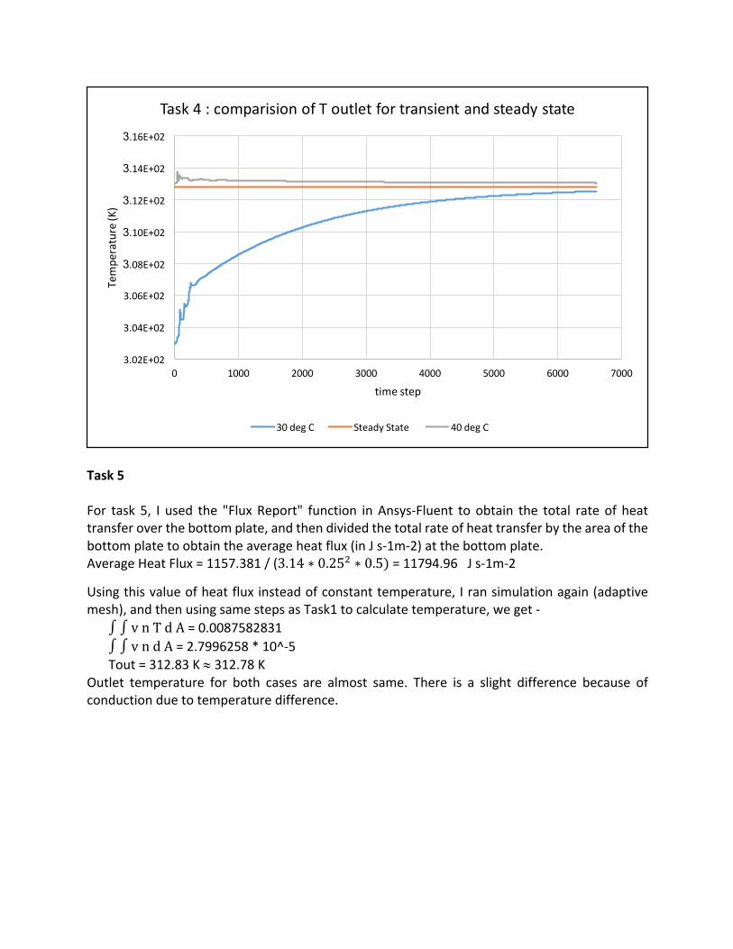
Task5For task 5, I used the "FluxReport" function inAnsys-Fluent to obtain the total rate of heattransferoverthebottomplate,andthendividedthetotalrateofheattransferbytheareaofthebottomplatetoobtaintheaverageheatflux(inJs-1m-2)atthebottomplate.AverageHeatFlux=1157.381/(3.14 ∗ 0.254 ∗ 0.5)=11794.96Js-1m-2

Usingthisvalueofheatfluxinsteadofconstanttemperature,Iransimulationagain(adaptivemesh),andthenusingsamestepsasTask1tocalculatetemperature,weget-

∫ ∫ vnTdA=0.0087582831∫ ∫ vndA=2.7996258*10^-5Tout=312.83K»312.78K

Outlet temperature for both cases are almost same. There is a slight difference because ofconductionduetotemperaturedifference.

3.02E+02

3.04E+02

3.06E+02

3.08E+02

3.10E+02

3.12E+02

3.14E+02

3.16E+02

0 1000 2000 3000 4000 5000 6000 7000

Tempe

rature(K)

timestep

Task4:comparisionofToutletfortransientandsteadystate

30degC SteadyState 40degC

contourplotoftemperatureonthebottomplate(bottomview)

contourplotoftemperatureonthebottomplate