Embed Size (px)
Citation preview

1
Informed Search and Exploration
Berlin Chen 2004
Reference:1. S. Russell and P. Norvig. Artificial Intelligence: A Modern Approach, Chapter 42. S. Russell’s teaching materials

2
Introduction
• Informed Search– Also called heuristic search– Use problem-specific knowledge– Search strategy: a node is selected for exploration based on an
evaluation function, • Estimate of desirability
• Evaluation function generally consists of two parts – The path cost from the initial state to a node n, (optional)– The estimated cost of the cheapest path from a node n to a goal
node, the heuristic function, • If the node n is a goal state →• Can’t be computed from the problem definition (need experience)
( )nf
( )nh
( )ng
( ) 0=nh

3
Heuristics
• Used to describe rules of thumb or advise that are generally effective, but not guaranteed to work in every case
• In the context of search, a heuristic is a function that takes a state as an argument and returns a number that is an estimate of the merit of the state with respect to the goal
• Not all heuristic functions are beneficial– Should consider the time spent on evaluating the heuristic
function– Useful heuristics should be computationally inexpensive

4
Best-First Search
• Choose the most desirable (seemly-best) node for expansion based on evaluation function– Lowest cost/highest probability evaluation
• Implementation– Fringe is a priority queue in decreasing order of desirability
• Several kinds of best-first search introduced– Greedy best-first search– A* search– Iterative-Deepening A* search– Recursive best-first search– Simplified memory-bounded A* search
memory-bounded heuristic search

5
Map of Romania
( )nh

6
Greedy Best-First Search
• Expand the node that appears to be closet to the goal, based on the heuristic function only
– E.g., the straight-line distance heuristics to Bucharest for the route-finding problem
•
• “greedy” – at each search step the algorithm always tries to get close to the goal as it can
( ) ( ) goalclosest the to node fromcost of estimate nnhnf ==
SLDh
( )( ) 366=AradInhSLD

7
Greedy Best-First Search (cont.)
• Example 1: the route-finding problem

8
Greedy Best-First Search (cont.)
• Example 1: the route-finding problem

9
Greedy Best-First Search (cont.)
• Example 1: the route-finding problem
– The solution is not optimal (?)

10
Greedy Best-First Search (cont.)
• Example 2: the 8-puzzle problem
2+0+0+0+1+1+2+0=6 (Manhattan distance )

11
Greedy Best-First Search (cont.)
• Example 2: the 8-puzzle problem (cont.)

12
Properties of Greedy Best-First Search
• Prefer to follow a single path all the way to the goal, and will back up when dead end is hit (like DFS)– Also have the possibility to go down infinitely
• Is neither optimal nor complete– Not complete: could get suck in loops
• E.g., finding path from Iasi to Fagars
• Time and space complexity– Worse case: O(bm) – But a good heuristic function could give dramatic improvement

13
A* Search
• Pronounced as “A-star search”
• Expand a node by evaluating the path cost to reach itself, , and the estimated path cost from it to the goal,– Evaluation function
– Uniform-cost search + greedy best-first search ?– Avoid expanding nodes that are already expansive
( ) ( ) ( )nhngnf +=
( )ng( )nh
( )( )( ) goal togh cost throupath totalestimated
from goal cost topath estimatedreach far to socost path
nnfnnh
nng
===
Hart, Nilsson, Raphael, 1968

14
A* Search (cont.)
• A* is optimal if the heuristic function never overestimates– Or say “if the heuristic function is admissible”– E.g. the straight-line-distance heuristics are admissible
( )nh
( ) ( )( ) goal to fromcost path true theis where
,*
*
nnhnhnh ≤
Finding the shortest-path goal

15
A* Search (cont.)
• Example 1: the route-finding problem

16
A* Search (cont.)
• Example 1: the route-finding problem

17
A* Search (cont.)
• Example 1: the route-finding problem

18
A* Search (cont.)
• Example 1: the route-finding problem

19
A* Search (cont.)
• Example 1: the route-finding problem

20
A* Search (cont.)
• Example 2: the state-space just represented as a tree
A
B C D
E F G L4
L1 L2 L3
4 3 2
3
2
4
1
8
1
3
Fringe (sorted)
Fringe Top Fringe Elements A(15) A(15) C(15) C(15), B(13), D(7) G(14) G(14), B(13), F(9), D(7) B(13) B(13), L3(12), F(9), D(7)
L3(12) L3(12), E(11), F(9), D(7)
Node g(n) h(n) f(n)A 0 15 15B 4 9 13C 3 12 15D 2 5 7E 7 4 11F 7 2 9G 11 3 14 L1 9 0 9L2 8 0 8L3 12 0 12L4 5 0 5
( ) ( ) ( ): node offunction Evaluation
nhngnfn
+=Finding the longest-path goal
( ) ( )nhnh *≥

21
Consistency of A* Heuristics
• A heuristic h is consistent if
– A stricter requirement on h
• If h is consistent
– I.e., is nondecreasing along any path during search
( ) ( ) ( ) ,, nhnancnh ′+′≤
n
n’
G
( )nanc ′,,( )nh
( ) nh ′
( ) ( ) ( )( ) ( ) ( )( ) ( )( )nf
nhngnhnancng
nhngnf
≥+≥
′+′+=
′+′=′
,,
( )nf
Finding the shortest-path goal
, where h(‧) is the straight-line distance to the nearest goal

22
Contours of the Evaluation Functions
• Fringe (leaf) nodes expanded in concentric contours
• Uniformed search ( )– Bands circulate around the initial state
• A* search – Bands stretch toward the goal and is narrowly focused around
the optimal path if more accurate heuristics were used
( ) 0 , =∀ nhn

23
Contours of the Evaluation Functions (cont.)
• If G is the optimal goal
– A* search expands all nodes with f(n) <f(G)
– A* search expands some nodes with f(n)=f(G)
– A* expands no nodes with f(n) > f(G)

24
Optimality of A* Search• A* search is optimal• Proof
– Suppose some suboptimal goal G2 has been generated and is in the fringe (queue)
– Let n be an unexpanded node on a shortest path to an optimal goal G
– A* will never select G2 for expansion since
( ) ( ) ( )( ) ( ) ( )( ) ( ) ( ) ( ) ( ))( admissible is since )(
lsuboptioma is since )(
0 since
*2
*222
nhnhh nhngnf
GnhngGg
GhGgGf
≤+=≥
+=>
==
( ) ( ) 2 nfGf >

25
Optimality of A* Search (cont.)
• Another proof– Suppose when algorithm terminates, G2 is a complete path (a
solution) on the top of the fringe and a node n that stands for a partial path presents somewhere on the fringe. There exists a complete path G passing through n, which is not equal to G2and is optimal (with the lowest path cost)
1. G is a complete which passes through node n, f(G)>=f(n) 2. Because G2 is on the top of the fringe ,
f(G2)<=f(n)<=f(G)3. Therefore, it makes contrariety !!
• A* search optimally efficient– For any given heuristic function, no other optimal algorithms is
guaranteed to expand fewer nodes than A*

26
Completeness of A* Search
• A* search is complete– If every node has a finite branching factor– If there are finitely many nodes with
• Every infinite path has an infinite path cost
• To Summarize again
( ) ( ) Gfnf ≤
Proof:Because A* adds bands (expands nodes) in orderof increasing , it must eventually reach a bandwhere is equal to the path to a goal state.f
f
( ) ( )( ) ( )
( ) ( ) with nodes no expands A with nodes smoe expands A
with nodes all expands A
*
*
*
GfnfGfnf
Gfnf
>
=
<
If G is the optimal goal

27
Complexity of A* Search
• Time complexity: O(bd)
• Space complexity: O(bd)– Keep all nodes in memory– Not practical for many large-scale problems
• Theorem– The search space of A* grows exponentially unless the error in
the heuristic function grows no faster than the logarithm of theactual path cost
( ) ( ) ( )( ) log- ** nhOnhnh ≤

28
Memory-bounded Heuristic Search
• Iterative-Deepening A* search
• Recursive best-first search
• Simplified memory-bounded A* search

29
Iterative Deepening A* Search (IDA*)
• The idea of iterative deepening was adapted to the heuristic search context to reduce memory requirements
• At each iteration, DFS is performed by using the-cost ( ) as the cutoff rather than the depth
– E.g., the smallest -cost of any node that exceeded the cutoff on the previous iteration
cutoff3
cutoff1
cutoff4 cutoffk
f hg +f
cutoff2
cutoff5

30
Iterative Deepening A* Search (cont.)

31
Properties of IDA*
• IDA* is complete and optimal
• Space complexity: O(bf(G)/δ) ≈ O(bd) – δ : the smallest step cost– f(G): the optimal solution cost
• Time complexity: O(αbd) – α: the number of distinct values small than the optimal goal
• Between iterations, IDA* retains only a single number –the -cost
• IDA* has difficulties in implementation when dealing with real-valued cost
f
f

32
Recursive Best-First Search (RBFS)
• Attempt to mimic best-first search but use only linear space– Can be implemented as a recursive algorithm– Keep track of the -value of the best alternative path from any
ancestor of the current node– It the current node exceeds the limit, the recursion unwinds back
to the alternative path– As the recursion unwinds, the -value of each node along the
path is replaced with the best -value of its children
f
ff

33
Recursive Best-First Search (cont.)
• Algorithm

34
Recursive Best-First Search (cont.)
• Example: the route-finding problem

35
Recursive Best-First Search (cont.)
• Example: the route-finding problem

36
Recursive Best-First Search (cont.)
• Example: the route-finding problem
Re-expand the forgotten nodes(subtree of Rimnicu Vilcea)

37
Properties of RBFS
• RBFS is complete and optimal
• Space complexity: O(bd)
• Time complexity : worse case O(bd)
– Depend on the heuristics and frequency of “mind change”– The same states may be explored many times

38
Simplified Memory-Bounded A* Search (SMA*)
• Make use of all available memory M to carry out A*
• Expanding the best leaf like A* until memory is full
• When full, drop the worst leaf node (with highest -value)– Like RBFS, backup the value of the forgotten node to its parent if
it is the best among the subtree of its parent– When all children nodes were deleted/dropped, put the parent
node to the fringe again for further expansion
f

39
Simplified Memory-Bounded A* Search (cont.)

40
Properties of SMA*
• Is complete if M ≥ d
• Is optimal if M ≥ d
• Space complexity: O(M)
• Time complexity : worse case O(bd)

41
Admissible Heuristics
• Take the 8-puzzle problem for example– Two heuristic functions considered here
• h1(n): number of misplaced tiles• h2(n): the sum of the distances of the tiles from
their goal positions (tiles can move vertically, horizontally), also called Manhattan distance orcity block distance
• h1(n): 8• h2(n): 3+1+2+2+2+3+3+2=18
42
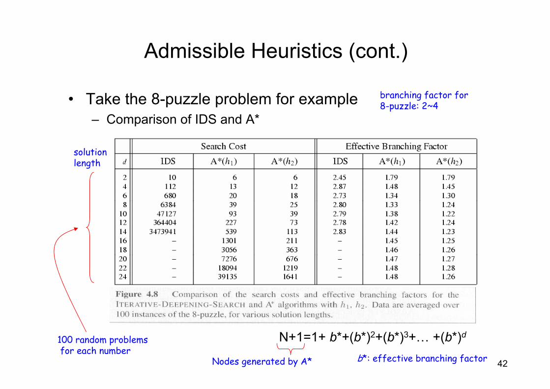
Admissible Heuristics (cont.)
• Take the 8-puzzle problem for example– Comparison of IDS and A*
100 random problemsfor each number
N+1=1+ b*+(b*)2+(b*)3+… +(b*)d
Nodes generated by A* b*: effective branching factor
branching factor for8-puzzle: 2~4
solutionlength

43
Dominance
• For two heuristic functions h1 and h2 (both are admissible), if h2(n) ≥ h1(n) for all nodes n– Then h2 dominates h1 and is better for search– A* using h2 will not expand more node than A* using h1
f(G)f(s)
f becomes larger
44
Inventing Admissible Heuristics
• Relaxed Problems– The search heuristics can be achieved from the
relaxed versions the original problem• Key point: the optimal solution cost to a relaxed problem
is an admissible heuristic for the original problem(not greater than the optimal solution cost of the original
problem)
– Example 1: the 8-puzzle problem• If the rules are relaxed so that a tile can move anywhere then
h1(n) gives the shortest solution• If the rules are relaxed so that a tile can move any adjacent
square then h2(n) gives the shortest solution

45
Inventing Admissible Heuristics (cont.)
– Example 2: the speech recognition problem
Original Problem(keyword spotting)
Relaxed Problem (used for heuristic calculation)
Note: if the relaxed problem is hard to solve, then the valuesof the corresponding heuristic will be expansive to obtain

46
Inventing Admissible Heuristics
• Composite Heuristics– Given a collection of admissible heuristics h1,h2,…,hm, none of
them dominates any of other
• Subproblem Heuristics– The cost of the optimal solution of the subproblem is a lower
bound on the cost of the complete problem
( ) ( ) ( ) ( ){ } ,...,,max 21 nhnhnhnh m=

47
Tradeoffs
Search Effort
Heuristic ComputationSearch Effort
Heuristic Computation
Heuristic ComputationSearch Effort
Search Effort
Heuristic Computation
Time
Relaxation of problemfor heuristic computation

48
Iterative Improvement Algorithms
• In many optimization, path to solution is irrelevant – E.g., 8-queen, VLSI layout, TSP etc., for finding optimal
configuration– The goal state itself is the solution– The state space is a complete configuration
• In such case, iterative improvement algorithms canbe used – Start with a complete configuration (represented by
a single “current” state)– Make modifications to improve the quality

49
Iterative Improvement Algorithms (cont.)
• Example: the n-queens problem– Put n queens on an nxn board with no queens on the same row,
column, or diagonal– Move a queen to reduce number of conflicts
(4, 3, 4, 3) (4, 3, 4, 2) (4, 1, 4, 2)
5 conflicts 3 conflicts 1 conflict

50
Iterative Improvement Algorithms (cont.)
• Example: the traveling salesperson problem (TSP)– Find the shortest tour visiting all cities exactly one– Start with any complete tour, perform pairwise exchanges
1 2
34
5
1→2→4→3→5→1 1→2→5→3→4→1
34
1 2
5

51
Iterative Improvement Algorithms (cont.)
• Local search algorithms belongs to iterative improvement algorithms– Use a current state and generally move only to the neighbors of
that state– Properties
• Use very little memory• Applicable to problems with large or infinite state space
• Local search algorithms to be considered– Hill-climbing search– Simulated annealing– Local beam search– Genetic algorithms
52
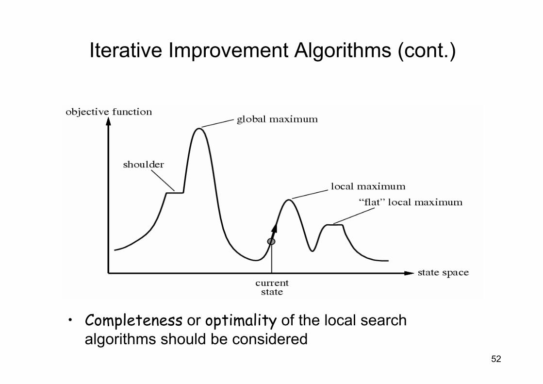
Iterative Improvement Algorithms (cont.)
• Completeness or optimality of the local search algorithms should be considered

53
Hill-Climbing Search
• “Like climbing Everest in the thick fog with amnesia”
• Choose any successor with a higher value (of objective or heuristic functions) than current state– Choose Value[next] ≥ Value[current]
• Also called greedy local search

54
Hill-Climbing Search (cont.)
• Example: the 8-queens problem– The heuristic cost function is the number of pairs of queens that
are attacking each other
– h=3+4+2+3+2+2+1=17 (calculated from left to right)
– Best successors have h=12 (when one of queens in Column 2,5,6, and 7 is moved)

55
Hill-Climbing Search (cont.)
• Problems:– Local maxima: search halts prematurely – Plateaus: search conducts a random walk– Ridges: search oscillates with slow progress
• Solution ?
Neither completenor optimal
8-queens stuck in a local minimum Ridges cause oscillation

56
Hill-Climbing Search (cont.)
• Several variants– Stochastic hill climbing
• Choose at random from among the uphill moves
– First-choice hill climbing• Generate successors randomly until one that is better than current
state is generated• A kind of stochastic hill climbing
– Random-restart hill climbing • Conduct a series of hill-climbing searches from randomly generated
initial states• Stop when goal is found
57
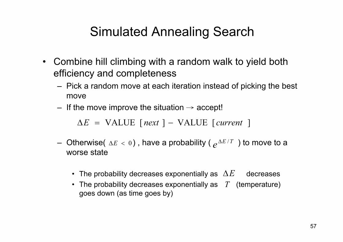
Simulated Annealing Search
• Combine hill climbing with a random walk to yield both efficiency and completeness– Pick a random move at each iteration instead of picking the best
move– If the move improve the situation → accept!
– Otherwise( ) , have a probability ( ) to move to a worse state
• The probability decreases exponentially as decreases• The probability decreases exponentially as (temperature)
goes down (as time goes by)
TEe /∆
E∆
][VALUE][VALUE currentnextE −=∆
T
0<∆E

58
Simulated Annealing Search (cont.)

59
Local Beam Search
• Keep track of k states rather than just one– Begin with k randomly generated states
– All successors of the k states are generated at each iteration
• If any one is a goal → halt!
• Otherwise, select k best successors from them and continue the iteration
– Information is passed/exchanged among these ksearch threads
• Compared to the random-restart search– Each process run independently

60
Local Beam Search (cont.)
• Problem– The k states may quickly become concentrated in a small region
of the state space– Like an expensive version of hill climbing
• Solution– A variant version called stochastic beam search
• Choose a given successor at random with a probability in increasing function of its value
• Resemble the process of natural selection

61
Genetic Algorithms (GAs)
• Developed and patterned after biological evolution
• Also regarded as a variant of stochastic beam search– Successors are generated from multiple current states
• A population of potential solutions are maintained
– States are often described by bit strings ( like chromosomes) whose interpretation depends on the applications
• Binary-coded or alphabet(11, 6, 9) → (101101101001)
• Encoding: translate problem-specific knowledge to GA framework
– Search begins with a population of randomly generated initial states

62
Genetic Algorithms (cont.)
• The successor states are generated by combining two parent states, rather then by modifying a single state
– Current population/states are evaluated with a fitness functionand selected probabilistically as seeds for producing the next generation
• Fitness function: the criteria for ranking• Recombine parts of the best (most fit) currently known states • Generate-and-test beam search
• Three phases of GAs– Selection → Crossover → Mutation

63
Genetic Algorithms (cont.)
• Selection– Determine which parent strings (chromosomes) participate in
producing offspring for the next generation
– The selection probability is proportional to the fitness values
– Some strings (chromosomes) would be selected more than once
( ) ( )( )∑ =
= P
j j
ii
hFitnesshFitnessh
1
Pr

64
Genetic Algorithms (cont.)
• Two most common (genetic) operators which try to mimic biological evaluation are performed at each iteration
– Crossover• Produce new offspring by crossing over the two mated parent
strings at randomly (a) chosen crossover point(s) (bit position(s))• Selected bits copied from each parent
– Mutation• Often performed after crossover• Each (bit) location of the randomly selected offspring is subject to
random mutation with a small independent probability
• Applicable problems– Function approximation & optimization, circuit layout etc.

65
Genetic Algorithms (cont.)
Encoding Schemes
Fitness Evaluation
Testing the End of the Algorithm
Parent Selection
Crossover Operators
Mutation Operators
HaltYES
NO

66
Genetic Algorithms (cont.)
• Example 1: the 8-queens problem
2 4 7 4 8 5 5 23 2 7 5 2 4 1 1 3 2 7 4 8 5 5 2
number of non attacking pairs of queens
parents offspring
( ) ( )( )∑ =
= P
j j
ii
hFitnesshFitnessh
1
Pr

67
Genetic Algorithms (cont.)
• Example 2: common crossover operators

68
Genetic Algorithms (cont.)
• Example 3: HMM adaptation in Speech Recognition
( )Dkkkk ,....,,, 3211 =h
( )Dmmmm ,....,,, 3212 =h
( ) ( ) ( ) ( )( )( ) ( ) ( ) ( )( )fDfffffff
fDfffffff
imikimikikimikim
ikimikimimikimik
−+⋅−+⋅−+⋅−⋅+⋅=
−+⋅−+⋅−+⋅−⋅+⋅=
1...., ,1 ,1 ,1
1,....,1 ,1 ,1
33322112
33322111
s
s
dg ddd gg σε ⋅+=ˆ
sequences of HMM mean vectors
crossover(reproduction)
mutation
( )
( )
( )∑ = ⎟
⎟
⎠
⎞
⎜⎜
⎝
⎛
⎟⎟⎠
⎞⎜⎜⎝
⎛
=P
j
j
i
i
TP
TP
1exp
expPr
hO
hO
h

69
Genetic Algorithms (cont.)

70
Genetic Algorithms (cont.)
• Main issues– Encoding schemes
• Representation of problem states– Size of population
• Too small → converging too quickly, and vice versa – Fitness function
• The objective function for optimization/maximization• Ranking members in a population

71
Properties of GAs
• GAs conduct a randomized, parallel, hill-climbing search for states that optimize a predefined fitness function
• GAs are based an analogy to biological evolution
• It is not clear whether the appeal of GAs arises from their performance or from their aesthetically pleasing origins in the theory of evolution

72
Local Search in Continuous Spaces
• Most real-world environments are continuous– The successors of a given state could be infinite
• Example: Place three new airports anywhere in Romania, such that the sum of squared distances from each cities to its nearest airport is minimized
x1,y1
x2,y2
x3,y3
objective function: f =?

73
Local Search in Continuous Spaces (cont.)
• Two main approach to find the maximum or minimum of the objective function by taking the gradient
1. Set the gradient to be equal to zero (=0) and try to find the closed form solution
• If it exists → lucky!
2. If no closed form solution exists• Perform gradient search !

74
Local Search in Continuous Spaces (cont.)
• Gradient Search– A hill climbing method– Search in the space defined by the real numbers– Guaranteed to find local maximum– Not Guaranteed to find global maximum
( ) ( )xxxxxx
ddff αα +=∇+=ˆ
maximization
minimization
( ) ( )xxxxxx
ddff αα −=∇−=ˆ
the gradient ofobjective function

75
Online Search
• Offline search mentioned previously– Nodes expansion involves simulated rather real actions– Easy to expand a node in one part of the search space and then
immediately expand a node in another part of the search space
• Online search– Expand a node physically occupied
• The next node expanded (except when backtracking) is the child of previous node expanded
– Traveling all the way across the tree to expand the next node iscostly

76
Online Search (cont.)
• Algorithms for online search– Depth-first search
• If the actions of agent is reversible (backtracking is allowable)– Hill-climbing search
• However random restarts are prohibitive– Random walk
• Select at random one of the available actions from current state• Could take exponentially many steps to find the goal