Informed Momentum Trading versus Uninformed Naive ... · Informed Momentum Trading versus Uninformed "Naive" Investors Strategies Anurag Banerjee and Chi-Hsiou ... For this purpose

Informed Momentum Trading versus Uninformed

"Naive" Investors Strategies

Anurag Banerjee�and Chi-Hsiou Hungy

Durham Business School

Abstract

We construct a zero-net-worth uninformed "naive investor" who uses a random

portfolio allocation strategy. We then compare the returns of the momentum strate-

gist to the return distribution of naive investors. For this purpose we reward momen-

tum pro�ts relative to the return percentiles of the naive investors with scores that

are symmetric around the median. The score function thus constructed is invariant

and robust to risk factor models. We �nd that the average scores of the momentum

strategies are close to zero (the score of the median) and statistically insigni�cant over

the sample period between 1926 and 2005, various sub-sample periods including the

periods examined in Jegadeesh and Titman (1993 and 2001). The �ndings are robust

with respect to sampling or period-speci�c e�ects, tightened score intervals, and the

imposition of maximum-weight restrictions on the naive strategies to mitigate market

friction considerations.

JEL: G11; G12; G14

�Durham Business School, Durham University.yDurham Business School, Durham University. Address for Correspondence: Email:

[email protected]; Tel: +44 191 334 5498; Address: Durham Business School, Mill Hill Lane,Durham, DH1 3LB, UK.

1

1 Introduction

There has been extensive research seeking to understand why the momentum strategies of

buying the recent winner stocks and selling short the recent loser stocks generate pro�ts as

documented by Jegadeesh and Titman (1993 and 2001). The risk-based approach, models

risk factors or dynamic risk exposures related to economic and �rm fundamentals. Many

studies demonstrate that momentum strategies, although reducing the exposure to the mar-

ket risk by undertaking the long-short positions, do not hedge risk in all dimentions and are

far from risk-free (e.g. Berk, Green and Naik (1999), Grundy and Martin (2001), Johnson

(2002), Pastor and Stambaugh (2003), Avramov and Chordia (2006), Chordia and Shivaku-

mar (2006), Sagi and Seasholes (2007) and Liu and Zhang (2008), among others). Some stud-

ies examine the momentum pro�ts after taking into account of transaction costs (Lesmond,

Schill and Zhou (2004), Korajczyk and Sadka (2004)) and liquidity (Sadka (2006)). Most

studies, however, show that model alpha of momentum strategies remains signi�cant1.

The approach using asset-pricing models requires correct speci�cations of risk factors

and the dynamics of time-varying coe¢ cients. If there is an omitted factor in a model,

the estimated alpha (and factor betas) su¤er from omitted variable bias. In this paper,

instead of investigating the potentially unidenti�ed factors, we propose a di¤erent approach

which removes the necessity of modeling risk to measure the performance of the momentum

strategies.

Our method rewards and penalizes the momentum strategist for using the past return

information in the formation of the strategies. To this end, we construct the "naive investors"

who use no information and weight risky assets randomly. The question we ask is, compared

1The theory and empirical evidence from behavioral approach advocate that the deviations from rationalbehavior can result in momentum (See, e.g. Chan, Jegadeesh and Lakonishok (1996), Barberis, Shleifer andVishny (1998), Hong and Stein (1999), Grinblatta and Han (2005), Hvidkjaer (2006) and Chui, Titman andWei (2010).

1

to the "naive investors", by how much do we reward or penalize the momentum strategist

for his/her e¤orts?

Imagine a stock market where there are both momentum investors (MI, hereafter) who

observe the past price pattern and "naive investors" (NI, hereafter) who do not. The traders

who pursue the zero net-worth momentum strategies must �rst observe past stock returns

in order to quantitatively form portfolios of the winner (top 10% past returns) and the

loser (bottom 10% past returns) stocks and then execute intensive long-short trading with

overlapping strategy positions.

The NIs, on the contrary, are agnostic about the return generating process, and hence do

not use any information. The NIs are unsophisticated and thus do not understand how to

sell short stocks2. They therefore randomly form long positions in the N risky assets. The

NIs invest in the same feasible set of stocks as that for constructing the momentum strategies

and �nance their investments in stock portfolios by borrowing at the risk-free rate, using

the one-month Treasury bill rate as a proxy. Thus, the NI�s strategies consist of both long

(the risky assets) and short (the risk-free asset) positions, thereby creating an initial zero

net-worth position. The excess portfolio returns from the naive strategies are thus the pro�ts

of the zero net-worth strategies of the naive investor.

To form a random portfolio, the uninformed NI chooses with equal chances any positive

or zero weight for each of the feasible stocks at the beginning of each month t. The weights �

of this portfolio, summing to unity, are thus a non-negative vector of random drawings from

an uniform distribution3. At the end of the period t, when asset returns r are realized the NI

liquidates his/her portfolio and gets a return of r0�: Since the portfolio weights are random

variables, the portfolio returns are also random variables. Therefore we get a probability

2Jones and Lamont (2002), for example, describe the di¢ culties of short sales including the risks, costs,legal and institutional restrictions, and the need of su¢ cient stock supply from investors who are willing tolend.

3We generate the portfolios using Monte Carlo method which is described in detail in Section 2.

2

distribution of returns of the NI at the end of period t. The NI then uses the same method

to reform and hold a portfolio for the next period t+1. We thus get the time-series of return

distributions of the NI.

Now consider the sophisticated MI who, unlike the NI, uses past return information to

form the momentum strategies FP at period t and gets the pro�t r0FP . Our method is

to compare the pro�ts r0FP of momentum strategies that buy the winners and sell short

the losers to the quintiles of the return distribution of the simple strategy of the NI. In

each period the MI gets a reward from the set of {2, 1, 0, -1 or -2}. If the pro�t r0FP is

above the 80th percentile of the return distribution of the NI, we assign a reward of 2 units.

Similarly, if it is above the 60th percentile but below the 80th percentile, an award of 1 unit

is assigned for the MI. Thus, the reward decreases with the quintiles. Likewise, below the

40th percentile and the 20th percentile of the NI return distribution the MI is penalized by

being awarded negative rewards of -1 and -2, respectively. Between the 40th percentile and

the 60th percentile the reward is zero4. We then generate a time-series of rewards over a

period of T years.

Note that by construction the median of the NI�s pro�ts is always awarded zero, and

that the rewards/penalties of the NI are uniformly distributed with a probability of 1/5.

Therefore, the expected reward of the NI is zero. Our hypothesis is that if the MI�s strategy

is better than the NI�s strategy, then he/she should, on average, get a positive reward for

the e¤orts over this T�year period. We test this hypothesis over di¤erent T�year horizons.

We call this function which assigns rewards to the MI by comparing r0FP to the NI return

distribution a score function. We show (in Theorem 1) and prove (in the Appendix) that

our method is appropriate because the score function is invariant under any common risk

4Note that the reward function does not have to be a �ve point function or even symmetric. Users canchange the parameters of this function.

3

factors in addition to scaling returns by volatility. That is, the scores of the risk-adjusted

returns of factor models are the same as those of the raw returns. Thus, the main advantage

of our method is that the score function does not require us to identify the source of risk

and to estimate factor loadings.

The second advantage of our method is that the score function is robust against return

outliers, and thus is robust against unexpected booms or busts of a group of companies.

Further, we can specify the level of robustness by estimation design. This advantage is

particularly useful since we �nd that there are extreme values of returns and pro�ts of the

momentum and the naive strategies. In contrast, most moment-based estimation techniques

are sensitive to outliers. For example, OLS has a breakdown point of 0% in that a change

of a single observation can change the parameter estimates.

Moreover, our score function is also useful as it provides robust statistical tests based on

it�s analytical and statistical properties: (i) The score function is invariant under common

a¢ ne transformation, i.e., that an overall increase or decrease in asset returns or a jump in

return volatility does not change the score of a strategy. Thus, the momentum strategies

do not receive rewards when everyone else in the market does as well; likewise, they are not

punished during a period of an overall market crash. (ii) The score function rewards and

penalizes a strategy, which can be directly used for performance management.

We also derive the asymptotic properties of the performance measure given a set of

asset returns, and then perform a t-test based on the asymptotic distribution of the score

function. If the momentum strategies outperform the naive strategies, the average score of

the momentum pro�ts should be signi�cantly positive.

We use the monthly equity data of the NYSE, AMEX and NASDAQ over the sample

period between 1926 and 2005, various sub-sample periods and 100 randomly selected ten-

year periods. In order to provide further detailes on the anatomy of the momentum trading,

4

we separately analyze the returns on the winner and the loser portfolios, and next look into

the momentum pro�ts from buying the winner and selling the loser portfolios. We �nd

that the winner portfolio has a small average score, positive and statistically signi�cant. In

contrast, although the losers generate negative returns that are statistically signi�cant, the

losers have a negative average score, but statistically insigni�cant. This is because the return

di¤erences between the losers and the NI�s have high variability and are small on average.

Strikingly, the average score of the momentum pro�ts from buying the winners and selling

the losers is close to zero. It is important to note that the scores of the momentum pro�ts

are not equal to the winners�scores minus the losers�scores as the scores are not linearly

additive. The momentum strategies take both sides of the extreme return positions, and

thus take up the tail risk. By doing so, they face large dispersions in the strategy pro�ts.

The momentum pro�ts are almost equally likely to either go higher than the 80th percentile

or drop below the 20th percentile of the pro�ts of the naïve investors strategies, and hence,

receive either the highest or the lowest scores at di¤erent points in time. As a result, the

scores of the momentum pro�ts o¤set each other. Overall results show that the momentum

strategies do not outperform the portfolios of the naïve investors.

Furthermore, in order to mitigate period-speci�c sampling considerations we simulate

the distributions of the average scores of the winner and the loser portfolios as well as the

momentum pro�ts by re-sampling with replacements for 100 times. In each of the 100

randomly chosen ten-year period we use all feasible stocks in the sample during that period

and then construct the empirical distribution of the average scores. Our simulations con�rm

the previous results.

Finally, since the naive investor might not be able to enjoy all the possible strategies

due to market frictions, we impose certain limits on the weight of a stock. This results

in evaluating the momentum strategy over a relatively restricted return space than the

5

unlimited one5. Since by construction, the naive investor is short in the risk-free asset to

establish the long position in stocks, we �rst set a maximum weight of 10% on each stock.

We also set a maximum weight of 10% on any stock in the smallest decile given their high

transaction costs. For robustness checks, we also apply a more detailed 11-point score system

based on the unrestricted return space and those with weight restrictions. These results are

quantitatively similar and do not change our conclusions.

Overall, we �nd that over the long-run the rewards and penalties cancel out and that

the momentum strategist is no better than a simple "naive" randomizer. Our �ndings

are important for a number of reasons. First, the evidence suggests that by 50% chance

the naive strategy would not perform worse than the momentum trading that is long the

winners and short the losers. From a practical point of view, asset managers who charge

fees and pursue the momentum strategies would have only 50% chance of beating the naive

strategies. Employing the information of past stock returns to form the momentum strategies

does not seem to be bene�cial as it requires costly and intensive trading. The construction

of the long-short strategy position is further complicated by the risks, costs and regulation

restrictions on short sales of stocks.

Second, the positive average score of the winner portfolio shows that by 60% of the time

the winner portfolio outperforms the naive strategies. Our evidence suggests that taking

a long position in the winner stocks which is �nanced at the risk-free rate can receive a

rather small, but positive reward. This, of course, does not take into account of the costs of

transactions, and of acquiring and analyzing return information.

The rest of the paper is structured as follows. Section 2 de�nes the strategies of the naive

investors. In Section 3 we construct a score function and describe the empirical tests. Section

5We are grateful to the anonymous referee for this valuable comment and the useful suggestions thatmake the analysis more interesting.

6

4 presents results and Section 5 concludes. The Appendix contains proofs of theorems,

statistical properties of the score function and derivations of statistical tests not presented

in the text.

2 The Naive Investors�Strategies

De�ne an investor�s portfolio strategy F over the asset set A which consists of N stocks that

are feasible for trading at a given time6 as

F : ! W (A)

where is the information available at the time of investing, W (A) is the vector of portfolio

weights on A chosen by an investor. The excess portfolio returns from strategy F is then

given by r0F where r is the vector of returns on the feasible asset set in excess of the risk-

free rate. Notice that FW , the strategy that selects winners, FL the strategy that selects

losers as well as the momentum strategy FP = (FW � FL) are in the set of W (A). For

the momentum investors, the information set is the past returns which they use to form

Winner and Loser portfolios.

We de�ne a naive investor (NI) as an agent who has an uninformed prior on asset returns

and does not change his portfolio formation decisions through acquiring information and

learning from own past investment outcomes. Since the NI does not use any information,

in each period, he randomly forms a vector of non-negative weights adding up to unity to

allocate his wealth to the set of feasible assets.6We supress the time-t subscript here to simplify notation.

7

Formally we de�ne the set of all possible strategies of the NI, �; as

� : fg ! W+ (A)

where fg denotes the empty information set employed by the NI. W+ (A) is the vector of

portfolio weights on the given feasible asset set A: This weight vector de�nes the feasible

portfolio set of the NI,

W+ (A) =nw : (wi) s.t. 0 � wi � 1 and

Xwi = 1; i = 1; 2; :::; N

o(1)

where wi is the weight on stock i 2 A. The feasible portfolios set is of N � 1 dimension

because of the restriction that the weights must sum to unity. In general this is also known

as an N dimensional unit simplex. W+ (A) forms an uniform distribution over the simplex.

For example, Figure 1 illustrates that the feasible portfolio set with three assets is a two

dimensional triangle, the vertices being (1, 0, 0), (0, 1 ,0) and (0, 0, 1).

[Insert Figure 1]

Also notice that FW and FL are in this set, i.e., fFW ;FLg 2 W+ (A) : We derive ana-

lytical expressions for the weights in Theorem A1 (see Appendix) which gives a method for

generating the weight distribution of the NI�s strategy uniformly over the unit simplex.

We emphasize that the random allocation by the NI means that the weights are randomly

drawn from an uniform distribution over a simplex, and hence, do not necessarily arrive at

an equally weighted portfolio. For example, in the 3-asset case the chance to allocate all

amount into only one asset with weights of (1, 0, 0) is the same as the chance to equally split

the investment amount with weights of (1/3, 1/3, 1/3) because the NI randomly chooses

weights (see Figure 1). In the Appendix we demonstrate the properties of the special case

8

where the NI chooses the same weight accross all feasible stocks to form an equally weighted

portfolio.

Let the cumulative distribution of the pro�ts of the NIs�strategies conditional on asset

returns, G (qj r), be given by

G (qj r) = Pr (r0� � qj r) :

Given the pro�t distribution we can then generate its percentiles qk such that G (qk j r) = k100;

k 2 f1; ::; 100g: In practice we do not need to compute the pro�t distribution since the weights

of the naive strategies can be simulated using Theorem A1.

To illustrate the density of the pro�ts (given in Theorem A2 in the Appendix) of the

NIs�portfolios, we use the 3-asset case as an example where the weights on the assets are

generated by Figure 1. Figure 2 plots the pro�t density g (qj r) of the NI�s when the returns

on the 3 assets are, respectively, -1%, 1% and 2%. It shows that the �rst quintile point, q20;

is 0.11%, the second point, q40; is 0.56%, ...etc.

[Insert Figure 2]

3 The Score Function

We de�ne a score function for a strategy F. Our objective is to evaluate the performance of

F with respect to the NIs�strategies. We give a score to a strategy based on the relative per-

formance of the excess portfolio returns r0F against the percentiles of the pro�t distribution

of the naive strategies.

9

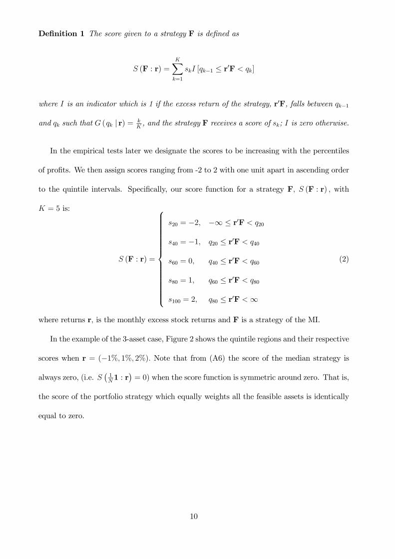
De�nition 1 The score given to a strategy F is de�ned as

S (F : r) =KXk=1

skI [qk�1 � r0F < qk]

where I is an indicator which is 1 if the excess return of the strategy, r0F, falls between qk�1

and qk such that G (qk j r) = kK, and the strategy F receives a score of sk; I is zero otherwise.

In the empirical tests later we designate the scores to be increasing with the percentiles

of pro�ts. We then assign scores ranging from -2 to 2 with one unit apart in ascending order

to the quintile intervals. Speci�cally, our score function for a strategy F; S (F : r) ; with

K = 5 is:

S (F : r) =

8>>>>>>>>>>>>>><>>>>>>>>>>>>>>:

s20 = �2; �1 � r0F < q20

s40 = �1; q20 � r0F < q40

s60 = 0; q40 � r0F < q60

s80 = 1; q60 � r0F < q80

s100 = 2; q80 � r0F <1

(2)

where returns r; is the monthly excess stock returns and F is a strategy of the MI.

In the example of the 3-asset case, Figure 2 shows the quintile regions and their respective

scores when r = (�1%; 1%; 2%): Note that from (A6) the score of the median strategy is

always zero, (i.e. S�1N1 : r

�= 0) when the score function is symmetric around zero. That is,

the score of the portfolio strategy which equally weights all the feasible assets is identically

equal to zero.

10

3.1 Analytical Properties of the Score Function

Assume that the cross-section of excess returns are characterized by a factor model:

rt = �t +Btxt + "t; "t ��0; �2t INt

�; t = 1; :::; T (3)

where �t = [�1t; :; �it;::; �Ntt], Bt = [�1t; ::;�it; :::;�Nt] is the vector of factor loadings, x0ts

are common risk factors, �2t is the cross-sectional variance at time t and Nt is the total

number of assets at time t. For a particular strategy Ft using equation (3) we get the usual

factor model

rF;t = �F;t + x0t�F;t + et; et �

�0; �2F;t

�(4)

where �F;t = �0tFt, �F;t = B0tFt, rF;t = r0tFt and �

2F;t = �

2tF

0tFt:

The following theorem states that the score function for measuring the performance of

a strategy is invariant under common risk factors, that is, the scores of the risk-adjusted

returns of a strategy are the same as those of the raw returns. This property is important

because, instead of identifying the �right factors�and measuring the risk-adjusted returns,

we can concentrate on raw returns for comparison purpose.

Theorem 1 Let the excess return generating process be given by the factor model (3). For

any strategy F 2 W (A) the score of the risk-adjusted return is the same as that of the excess

return,

S

�F :

r�Bx�

�= S (F : r) :

The theorem also gives an additional practical advantage over traditional methods of

estimating the risk factor model. If there are omitted factors xt in a model of (4), the

estimates of �F;t will be biased. This has led to considerable research in identifying the right

factors, for example, the factors of the market (the CAPM), the SMB and HML (Fama-

11

French (1993)), liquidity (Pastor and Stambaugh (2003)), macroeconomic risk (e.g., Liu and

Zhang (2008)) and momentum (e.g., Avramov and Chordia (2006)). Theorem 1 implies that

we can avoid the identi�cation of risk factors and hence, the estimation of factor loadings

�F;t.

Theorem 2 The score function has a breakdown point7 of 100K% when q1 = �1 and/or

qK = +1:

Theorem (2) shows that our score function is robust against outliers and structural shifts

in the return data. By construction, only when a fraction of 100K% of the data taking arbitrary

values (such as outliers or data shifts) would the score function change. In our empirical

analysis later, we choose K = 5 i.e a break down point of 20%.

In contrast, conventional moment-based estimators are sensitive to changes in sample

observations in that the point estimate of a model will change even if only one �rm is

removed from the sample. For example, if we estimate model (4) using OLS method, a

bankruptcy of just one �rm can change the value of the estimate of �F;t: Indeed, moment-

based regression methods have the same problem. Least Squares Median estimator has a

breakdown point of 50%, but lacks precision, and also typically fares even worse than OLS

for cases with high leverage points8. Bounded in�uence methods have a high breakdown

point but they e¤ectively remove a large proportion of observations.

Part a) of the following theorem shows that the strategy of shorting the loosers for our

symmetric 5 point strategy function receives a score of S (�FL : r) = �S (FL : r) :

7Breakdown point of a statistic is the smallest fraction of �bad�data (outliers or data grouped at theextreme of a tail) the statistic can tolerate without taking on values arbitrarily far away from uncontaminatedstatistic (for details see: Huber and Ronchetti (2009))

8Outliers with respect to the predictors are called leverage points (for details see: Belsley, Kuh and Welsch(1980))

12

Theorem 3 a) If the score function is symmetric i.e. sk = �sK�k+1, for k = 1; ::; K then

S (�F : r) = �S (F : r)

b) If sk�1 � sk for all k, for two strategies F1 and F2 where S (F1 : r) � S (F2 : r) ; we

have

S (F1 : r) � S (�F1 + (1� �)F2 : r) � S (F2 : r)

for all � 2 (0; 1) :

Since the score function in a step-function of strategy returns, it is non linear. Thus,

scores of the momentum pro�ts from buying the winners and selling short the losers are not

always equal to the winners�scores minus the losers�scores, i.e., S (FP : r) 6= S (FW : r) �

S (FL : r) :9

3.2 Sample and Empirical Tests

We use monthly equity data of the NYSE, AMEX and NASDAQ �les from the Center

for Research in Security Price (CRSP) for the period between January 1926 and December

2005. Our tests focus on the representative momentum strategies that form equally weighted

portfolios by sorting stocks on their past 6-month compounded returns and hold portfolios

for 6 months. We exclude all stocks with prices below $5 at portfolio formation as in

Jegadeesh and Titman (1993). This de�nes our feasible asset set A. At the end of each

month, the stocks within the top 10% of past returns comprise the winner portfolio and

stocks within the bottom 10% of past returns comprise the loser portfolio. The overlapping

momentum strategies thus consist of six strategies with each starting one month apart.

9As a counter example, suppose 0 < S (F1 : r) < S (F2 : r) ; then r0F1 < r0F2: Without loss of generalitylet r0F1 = 0; then S (F1 + F2 : r) = S (F2 : r) 6= S (F1 : r) + S (F2 : r) :

13

Portfolios are initially equally weighted at the time of formation and are held for six months

without rebalancing during the holding period10. We compute monthly excess portfolio

returns and the pro�ts to momentum strategies using single-period returns as in Liu and

Strong (2008). The monthly portfolio returns from the overlapping strategies are averages

of the six strategies as in Jegadeesh and Titman (1993).

One of the reasons for developing a score function to compare the momentum strategies

against the entire distribution of the strategies of NIs is that a standard t-test is not robust

against return outliers. Indeed, over the whole sample period the kurtosis of the momentum

pro�ts is 33. The Jarque-Bera test rejects the normality assumption for the momentum

pro�ts (the p-value is essentially zero).

We generate the distribution of the cross-section of excess portfolio returns. Using the

result in Theorem (A1) we construct, each month, a cross-section of excess returns of 1,000

portfolios for the NIs and obtain the quintile points of the excess return distribution. We

then assign scores as described in equation (2).

To illustrate the score distribution we plot Figure (3) which shows in box charts the

monthly pro�t distribution of the NIs�strategies for the period from 1990 to 1998 examined

by Jegadeesh and Titman (2001). The bottom box displays the 20th to the 40th percentiles

of the excess returns of the NIs strategies; the green box in the middle displays the 40th to

the 60th percentiles; and the top box displays the 60th to the 80th percentiles.

[Insert Figure 3 here]

Using the centered excess returns rc = r�r1 we plot the centered box charts in Figure

4. Corollary A4 shows that the score function is a¢ ne invariant in returns, i.e., S (F : r) =

S (F : rc). One signi�cant observation is in order, the distribution of the centered returns

10In the case when a stock is delisted during the holding period, the liquidating proceeds are reinvestedin the remaining stocks in the portfolio.

14

is stable, and hence is the score function. We also plot the �gures (unreported for brevity,

but available upon request) for the periods from 1965 to 1989 of Jegadeesh and Titman

(1993), and the period from 1999 to 2005, respectively. The patterns in these �gures are

qualitatively the same and show that the distributions of the centered returns are stable.


The empirical average score of the strategy Ft is given by:

b� (fFt : rtg) = 1

T

TXt=1

St (fFt : rtg) :

The mean of the average scores b� (f�t : rtg) using the results from (A8) when the score

function is given by (2) or any symmetric score function is given by:

E [b� (f�t : rtg)] = 0.We use the score function (2) to evaluate the momentum strategies. The winner and the

loser portfolios and the momentum strategies receive a score of zero if their excess returns

or pro�ts fall within the 40th and the 60th percentiles of the excess return distribution of

the NIs strategies; a score of 1 for falling within the 60th and the 80th percentiles; and a

score of 2 for going higher than the 80th percentile. The negative scores are given vice versa.

We then use the score function to evaluate the momentum pro�ts and the excess returns on

the winner and the loser portfolios. Appendix C gives details for the statistical tests of the

scores.

Our goal is to �nd out whether the scores of momentum pro�ts are signi�cantly higher

than those of the NIs�strategies. Therefore we test the null hypothesis H0 : E[S (FP : r)] = 0

against the alternative HA : E[S (FP : r)] > 0: We evaluate the score of the momentum

15

strategies every month during the T evaluation periods and then calculate the average score,

b� (fFPt : rtg) : Therefore a test of whether the momentum strategies outperform the NIs

strategies is to test whether the average score of the momentum strategies is signi�cantly

positive. We perform a test based on the t-test given by (A9) in the Appendix. We also run

the tests for the winner H0 : E[S (FW : r)] = 0 (against HA : E[S (FW : r)] < 0): We noted

before that shorting the losers will gives positive scores (see Theorem 3 a)). Therefore we

test whether the score of the loser portfolios is negative i.e. H0 : E[S (FL: r)] = 0 against

HA : E[S (FL: r)] < 0.

4 Results

Table 1 presents the average scores of the winner, the loser portfolios and the momentum

pro�ts. Panel A shows, for the whole sample period, that the winner portfolio has a small, but

positive and statistically signi�cant average score of 0.11; the loser portfolio has a negative

and statistically signi�cant average score of -0.09. The average score of the momentum

pro�ts is 0.02 and statistically insigni�cant, showing that the momentum strategies do not

outperform the zero net-worth strategies of the NIs.

[Insert Table 1 here]

Figure 5 shows the relative frequencies of the scores. In Panel A for the whole sample

period, the scores of the winner, the loser portfolios and the momentum pro�ts tend to be

at the extreme ends of either positive or negative 2. The excess returns on the winner and

loser portfolios are more likely to receive positive and negative extreme scores, respectively.

In contrast, the chances for the momentum pro�ts to receive either positive or negative 2

are very close (0.468 versus 0.483), thereby o¤setting each other. As a result, the average

score of the momentum pro�ts is close to zero, which corresponds to the results in Table 1.

16


4.1 Over Sub-Sample Periods

We then perform the analysis for various sub-sample periods. Panel B of Table 1 shows that

over the period between 1965 and 1989 as in Jegadeesh and Titman (1993), both the average

scores of the winner and the loser portfolios are very low and statistically insigni�cant. The

average score of the momentum pro�ts is essentially zero and statistically insigni�cant. The

results in Panels C, D and E for the sample periods of Jegadeesh and Titman (2001), the

period between August 1929 and March 1933 during the great depression as designated by

the NBER, and the period between January 1995 and March 2000 for the dot-com bubble,

respectively, show very similar patterns. Overall, the average scores of the momentum pro�ts

are close to zero in all the periods considered.

Panels B and C of Figure 5 show respectively, the score frequencies for the periods

of Jegadeesh-Titman (1993 and 2001). The scores of the winner, the loser portfolios and

the momentum pro�ts exhibit very similar patterns as in Panel A. Panels D and E show,

respectively, the score frequencies for the periods during the great depression and the dot-com

bubble. Comparing to the other periods examined, during the great depression period the

cases of extremely positive and negative returns on the winner portfolio occur less frequently

while the loser portfolio is more likely to generate extreme losses. Therefore, the momentum

strategies that buy winners and sell short losers are more likely to receive a score of +2.

During the dot-com bubble the loser portfolio seems to become less likely to generate extreme

losses. Again, the momentum pro�ts have extreme scores on both ends, o¤setting each other.

To understand this phenomenon, in Figure 6 we plot the box charts for the momentum

pro�ts for the period between 1990 and 1998.11 The blue lines above the top boxes show

11To avoid ambiguity in the graph we only show the charts over this short period for clear illustration. The

17

the magnitudes of the momentum pro�ts going higher than the 80th percentiles of the

distributions of the excess returns of the NIs strategies. The red lines below the bottom

boxes show the magnitudes of the momentum pro�ts being lower than the 20th percentiles.

An observation is clear that the momentum strategies incur high levels of pro�ts and loses

from time to time, but overall, are likely to o¤set each other.


This phenomenon is better illustrated in Figure 7 where we plot the box charts for the

momentum pro�ts using the distribution of centered excess returns rc which subtract r from

r: Note that the magnitudes of the momentum pro�ts displayed here are the same as those

in Figure 6.12 Interestingly, we �nd that there are very few periods of momentum pro�t

runs i.e. consecutive months of large positive pro�ts, highlighting the risky nature of the

momentum trading.


4.2 100 Randomly Selected 10-Year Periods

We design a simulation experiment to see whether the momentum strategies outperform the

naive strategies in any given period and any given set of assets. For each run, we select an

experiment period of 120 months with the starting month randomly chosen between July

1926 and December 1995. We then use all sample stocks in that period and the portfolio

formation methods described earlier to form the momentum strategies and the strategies of

the NIs. The set of sample stocks that are used to construct NIs portfolios is the same as

results (available upon request) for the whole sample period and other sub-sample periods are qualitativelyvery similar and do not change the conclusions.12

r0cFP = (r�r1)0(FW � FL) = r (FW � FL) since 10FW = 10FL = 1:

18

that of the momentum portfolios. We compute average excess returns of the momentum

portfolios and the monthly pro�t distributions of the zero net-worth naive strategies over

the 120 months.

In a randomly selected sample we give a score to the momentum strategies, i.e., b� (fFjt : rtg) ;j = W;L; P in each month and then compute an average score over 120 months in the sam-

ple. We sample 100 times with replacements and then generate 100 average scores for each

of the winner and the loser portfolios as well as the momentum pro�ts.

The winner portfolio tends to receive positive average scores, while the average scores of

the loser portfolio are positively skewed and tend to be negative. We test, in each sample,

whether the average scores of the momentum pro�ts are positive. Speci�cally, we test the

null hypothesis of H0 : E[S (FP : r)] = 0 against the alternative of E[S (FP : r)] > 0 using

the 120 monthly scores of the momentum pro�ts: At the 5% level 82% of the samples accept

the null. Hence, the naive diversi�er is almost as good as the momentum strategist. The

results demonstrate that the momentum strategies do not outperform the strategies of the

NIs in the randomly selected samples, consistent with the results in the earlier sections.

4.3 Robustness Checks

4.3.1 Imposing Weight Restrictions on the NI�s Portfolio

We impose some restrictions on the naive investors�strategies in order to examine the ro-

bustness of our results in a more realistic setting than the unrestricted one we examined

earlier. The �rst restriction is that the weight on each stock in the naive investor�s portfolio

cannot exceed a maximum of 10%. Speci�cally, the feasible set is now given by:

W(1)+ (A) =

nw : 0 � wi � 0:1 for all i 2 A and

Xwi = 1

o: (5)

19

Consequently, the chance for the naive investor to place an excessively large weight on

a stock that experiences an extreme return during the holding period is eliminated, leading

to a shrinkage in the tails of the pro�t distribution of the naive strategies. Therefore, those

momentum returns falling within the range between the 80th and the 20th percentiles in the

previous analysis are now possible to fall outside of this range, and hence receive extreme

scores on both ends.

Notice that, however, since most of the momentum returns in the previous analysis

are already outside of the range between the 80th and the 20th percentiles, they continue to

either drop below the 20th percentile or go higher than the 80th percentile of the naive pro�t

distribution after applying for the restriction. Again, we �nd that the momentum strategies

receive extreme scores at di¤erent points in time, and cancel out each other accross time.

Part I of Table 2 reports the results. Over the whole sample period both the winner

and the loser portfolios have rather small, but statistically signi�cant average scores. The

extreme positive and negative scores for the momentum pro�ts o¤set each other. Thus, the

average score of the momentum pro�ts is close to zero and statistically insigni�cant. Overall

results for various sub-periods, again, con�rm our �ndings reported earlier.


Given the typically high transaction costs of small size stocks, we exam the second re-

striction that the weight of the naive investor�s portfolio on a stock whithin the smallest size

decile of the feasible asset set cannot exceed a maximum of 10%. This implicitly implies an

assumption that the naive investor has the information on �rm size. Formally we de�ne the

set of all possible strategies of the NI, �; as

� : fMVi; i 2 Ag ! W(2)+ (A)

20

whereMVi is the market value of asset i: The weight vector that de�nes the feasible portfolio

set of the NI is

W(2)+ (A) =

nw : 0 � wi � 0:1 for all i s.t. MVi � q10 (MV ) and

Xwi = 1

o(6)

where q10 (MV ) is the bottom decile of the market values of all feasible stocks.

We randomly choose weights w; as in (1) and use an Acceptance-Rejection algorithm 13

to restrict our weights in the feasible sets de�ned in (5) and (6). Overall results reported in

Part II of Table 2 con�rm our �ndings over the whole sample period and various sub-periods.

Again, we �nd that the momentum strategies receive extreme scores at di¤erent points in

time, and cancel out each other accross time.

4.3.2 Using 11 Points Score Function

We repeat the empirical tests using 11 score points of the return distribution by assigning

scores ranging from -5 to +5 with one unit apart in ascending order of equal intervals of 9:1

(i.e. 100/11) percentiles. Speci�cally, our score function for a strategy F; eS (F : r) ; withK = 11 can be written compactly as:

eS (F : r) = 11Xk=1

(k � 6) Ihq 100�(k�1)

11

� r0F < q 100�k11

i(7)

where q� is ��percentile of the NI�s returns and r0F is the return of the MI. It is worth to

note that the choice of odd-number points for a score function ensures that the median of

the naive strategies always gets zero score.

Part I of Table 3 presents the results. The only di¤erence in results from using a 11-point

score system is that both the winner and the loser portfolios now have insigni�cant average

13See Robert and Casella (2004) for details.

21

scores over the whole sample period. This is a result of increasing the variance of the scores

because the scores now can take 11 points instead of 5 points in the earlier analysis.


Figure 5 further gives the relative frequencies of the scores over various periods we exam-

ined. The overall pattern reveals that the scores of the winner portfolio, the loser portfolio

and the momentum pro�ts tend to be at the extreme ends of either positive or negative 5,

providing further evidence that momentum returns often locate at the tails of the naive re-

turn distribution. Again, the extreme positive and negative scores for the momentum pro�ts

o¤set each other, resulting in an average score close to zero.


Parts II and III of Table 3 report the results, respectively, for the analyses of applying the

�rst restriction of a maximum weight of 10% on each stock and the second restriction of a

maximum weight of 10% on small size stocks. In all cases, the winner and the loser portfolios

show small (of opposite signs) and statistically insigni�cant average scores. The average

scores of momentum pro�ts are close to zero and statistically insigni�cant. Overall, the

results from applying such restrictions are very similar to those of the case with unrestricted

weights and do not change our conclusions.

5 Conclusions

In this paper we evaluate the pro�ts of the momentum strategies which use past return

information against the cross-section of the pro�t distribution of the zero net-worth strategies

of "naive investors" (NIs) who do not use any information. We de�ne a score function which

is invariant under di¤erent risk factors, and by which to give scores to the momentum

22

strategies relative to the pro�ts of the population of the NIs. We thus do not need to

specify the risk factors underlying the momentum e¤ect. We �nd that average scores of

the momentum strategies are close to zero and statistically insigni�cant over the sample

period between 1926 and 2005, various sub-sample periods including the periods examined

in Jegadeesh and Titman (1993 and 2001). The �ndings are robust with respect to sampling

or period-speci�c e¤ects in our simulations where we randomly select 10 years for 100 times.

Our overall results are also robust to the use of a more detailed score system, or maximum

weight restrictions on stocks. The preponderance of the evidence suggests that professional

asset managers who pursue the momentum strategies would have only 50% chance of beating

the naive strategies.

Appendix

A Proofs of Theorems

Theorem A1 The joint distribution of the portfolio weights of the NI is uniform and is

given by � = (�1; :::; �i; :::; �N) where the marginal distribution of the weight on stock i is

�i =EiPEi, and Ei s iid ExponentialDist(1) such that the density of � is

h (w) = N !; if w 2 W+ (A) ;

= 0; otherwise

Proof of Theorem. A1: First note thatPN

i=1 �i = 1 and 0 � �i � 1 for all i = 1; :::N:

We prove that the joint density of � is a constant.

23

Let E =PN

i=1Ei and the joint density of Ei �s is: exp��PN

i=1 ei

�. Therefore the joint

density of (E1; ::; Ei; ::EN ; E) is given by :

exp

�

NXi=1

ei

!I

"NXi=1

ei = e

#:

Consider the reverse transformation Ei = E�i: The Jacobian of the transformation is EN :

Thus the joint density of (�; E) is ceN exp (�e), where c is a normalizing constant: Integrat-

ing out e and normalizing the constant gives h (w) = N !:

Corollary A1 The cross-sectional mean and the projection median, PM; 14 of � are given

by

E[�] = PM (�) =1

N1 (A1)

where 1 is a vector of ones with length N .

Corollary A2 The variance-covariance matrix of � is

E[��0] = �� =1

N (N + 1)

�I� 1

N110�: (A2)

Corollary A3 The excess portfolio return from a naive strategy � is given by r0�: Following

from (A1), the cross-sectional mean and the median of the excess portfolio returns of the NI

strategies are

E[r0�] =M (r0�) =1

N

NXi=1

ri = r

Hence, r is e¤ectively the equally weighted excess return of the feasible asset set. From (A2)

14See: Zuo (2003) for a recent discussion.

24

the variance of the excess portfolio returns of the NI strategies is

V ar (r0�) =1

N + 1

NXi=1

(ri � r)2 :

Theorem A2 Let g be the density of the pro�ts of the NIs�strategies such that G (qj r) =qZ

�1

g (qj r) dz, where r is a vector of excess returns. We have:

g (qj r) =NXk=1

(rk � q)N�1NY

l=1;l 6=k

(rl � rk)

Proof of Theorem. A2: We can write

G (qj r) = Pr

NXi

riEi � qNXi

Ei

!= Pr

NXi

(ri � q)Ei � 0!

(A3)

The density of Y =PN

i (ri � q)Ei at y = 0 follows from equations (27) and (28) of Biswal

et. al. (1998, pages 593-594) by substituting �ij = 1 and xk = (ri � q).

Proof of Theorem. 1: Note that

G (q : r) = Pr (r0� � q) = Pr�r0�� (�+Bx)0F

�� q � (�+Bx)0F

�

�:

then

S (F : r) =

KXk=2

skI [qk�1 � r0F < qk]

=

KXk=1

skI

�qk�1 � x0B0F

�� r0F� x0B0F

�<qk � x0B0F

�

�= S

�F :

r�Bx�

�:

25

As a special case we get the following corollary.

Corollary A4 The score function is invariant under common a¢ ne transformation i.e.,

for any � 2 R+ and � 2 R, the score of a¢ ne transformations of the excess returns remains

the same.

S (F : �r+ �1) = S (F : r) :

Proof of Theorem. 2: It is easy to see that since we are using kth percentiles, N=K

returns in r needs to be arbitrarily large to change the score function.

Proof of Theorem. 3: a) Notice that Pr(r0� �qa (r0�)) = �() Pr(�r0� � �qa (r0�)) =

1 � �, implying that �qa (r0�) = q1�a (�r0�) : Now because of the symmetry of the scores

we have:

S (�F : r) =KXk=1

skI [qk�1 � �r0F < qk]

=KXk=1

skI [�qk�1 � r0F > �qk]

=KXk=1

�sK�kI [qK�k � r0F < qk] = �S (�F : r) :

b) Note that S (F : r) =PK

k=1 skI [qk�1 � r0F < qk] is an increasing function of r0F,

and is both quasi-concave and quasi-convex in r0F. Hence, if S (F1 : r) � S (F2 : r) ; then

r0F1 � r0F2

S (F1 : r) =KXk=1

skI [qk�1 � r0F1 < qk]

�KXk=1

skI [qk�1 � r0 [�F1 + (1� �)F2] < qk]

�KXk=1

skI [qk�1 � r0F2 < qk] = S (F2 : r) :

26

B Statistical Properties of the Score Function

Given an excess return vector r; the probability of strategy F receiving a score sk is

pk � Pr (S (F : r) = sk) � Pr (qk�1 � r0F < qk)

Thus, the expected score of the strategy is

E[S (F : r)] = �S (F : r) =KXk=1

skpk (F : r) = s0p:

where p = [p1 (F : r) ; ::pk (F : r) ::; pK (F : r)] is the vector of probabilities that strategy F

receives the designated scores s =(s1; ::sk::; sK) for its returns falling in the corresponding

return ranges: The variance of the scores of strategy F is

V ar (S (F : r)) = �2S (F : r) =KXk=1

[sk]2 pk (F : r)� [�S (F : r)]

2 : (A4)

The mean and variance of the scores for the NI strategy � are, respectively:

�S (� : r) =1

K

KXk=1

sk; and �2S (� : r) =1

K

KXk=1

[sk]2 � [�S (� : r)]

2 (A5)

Normalizing the expected score of the NI strategy to be zero by choosing appropriate s,

the variance is then simply �2S (� : r) =1K

PKk=1 [sk]

2 : The median of the score of the NI

strategy is

M(S (� : r)) = sm; such that qm�1 � r < qm: (A6)

27

Recall that the median strategy is feasible as the equally weighted portfolio 1N1 and thus

always has a score of sm; i.e., S�1N1 : r

�= sm: The variance of the equally weighted portfolio

is zero, i.e.,V ar�S�1N1 : r

��= 0:

C Tests of Statistical Signi�cance of the Scores

We test the null hypothesis H0 : E[S (F : r)] = E[S (� : r)] against the alternative H1 :

E[S (F : r)] > E[S (� : r)]: The empirical average score of any strategy Ft is given by:

b� (fFt : rtg) = 1

T

TXt=1

S (fFt : rtg) :

In order to construct a test statistic for the purpose under the null hypothesis we �nd

the sampling distribution of the average score under the null i.e. b� (f�t : rtg) where �t and

rt are the naive strategy and the vector of excess stock returns at period t = 1; :::; T: The

likelihood function of the scores of the naive strategies is a multinomial distribution:

L (� 1; :::; �K : f�t; rtg) = cKYk=1

p�kk

where � k =TPt=1

I [qk�1;t � r0t�t < qk;t] is the number of times the naive strategy return r0t�t

falls between qk�1;t and qk;t where qk;t is the k=K percentile of the excess return distribution

of the naive strategy at period t, such thatP� k = T and c is a normalizing constant.

The maximum likelihood estimator (MLE) for pk is then given by: bpk = �kT: The asymp-

totic distribution of bpk ispT bpk asy� N (pk; pk (1� pk)) ; k = 1; :::; K:

28

The variance and covariance of bpk arevar (bpk) = pk (1� pk)

Tand Cov (bpk; bpl) = �pkpl

T:

Therefore, from (A5), the empirical mean of the scores is

b�S (fFt : rtg) = KXk=1

skbpkThe expectation of b�S (f�t : rtg) and the sample variance of b�S (f�t : rtg) are

E[b�S (f�t : rtg)] = KXk=1

skpk and V ar (b�S (f�t : rtg)) = �2S (�t: r)

T: (A7)

From the discussion above, the asymptotic properties of the performance measure for naive

strategy �t given a vector of asset returns rt at period t is

pTb� (f�t : rtg) asy� N

��S (� : r) ; �

2S (� : r)

�: (A8)

Therefore the di¤erence in performance between strategy F and the NI strategy � can be

measured by b� (fFt : rtg)� � (� : r) : One can compute a t-ratio using (A8) for testing thenull hypothesis that strategy F performs the same as the NI strategy � as

t (F) =pTb� (fFt : rtg)� �S (� : r)p

�2S (F : r): (A9)

29

References

Avramov, Doron, and Tarun Chordia, 2006, Asset Pricing Models and Financial MarketAnomalies, Review of Financial Studies, 19, 1001-1040.

Barberis, N., A. Shleifer and R. Vishny, 1998, A Model of Investor Sentiment, Journal ofFinancial Economics, 49, 307�343.

Belsley, David A., Edwin Kuh and Roy E. Welsch, (1980), Regression Diagnostics: Identi-fying In�uential Data and Sources of Collinearity, John Wiley & Sons Inc.

Berk, Jonathan B., Richard C. Green, and Vasant Naik, 1999, Optimal Investment, GrowthOptions, and Security Returns, Journal of Finance, 54, 1153-1607.

Biswal, Mahendra P, N. Biswal, and Duan Li, 1998, Probabilistic Linear ProgrammingProblems with Exponential Random Variables: A Technical Note, European Journalof Operational Research, 111, 589-597.

Chan, Louis K., Narasimhan Jegadeesh, and Josef Lakonishok, 1996, Momentum Strategies,Journal of Finance, 51, 1681-1713.

Chordia, Tarun, and Lakshmanan Shivakumar, 2006, Earnings and Price Momentum, Jour-nal of Financial Economics, 80, 627�656.

Chui, Andy C., Sheridan Titman, and K. C. John Wei, 2010, Individualism and Momentumaround the World, Journal of Finance, 65, 361-392.

Fama, Eugene F., and Kenneth R. French, 1993, Common Risk Factors in the Returns onStocks and Bonds, Journal of Financial Economics, 33, 3-56.

Grinblatta, Mark, and Bing Han, 2005, Prospect Theory, Mental Accounting, and Momen-tum, Journal of Financial Economics, 78, 311�339.

Grundy, Bruce D., and Spencer J. Martin, 2001, Understanding the Nature of the Risksand the Sources of the Rewards to Momentum Investing, Review of Financial Studies,14, 29-78.

Hong, Harrison, and Jeremy C. Stein, 1999, A Uni�ed Theory of Underreaction, MomentumTrading and Overreaction in Asset Markets, Journal of Finance, 54, 2143�2184.

Huber, Peter J. and Elvezio Ronchetti, 2009, Robust Statistics, John Wiley & Sons Inc.

Hvidkjaer, Soeren, 2006, A Trade-Based Analysis of Momentum, Review of Financial Stud-ies, 19, 457-491.

Jegadeesh, Narasimhan, and Sheridan Titman, 1993, Returns to Buying Winners and Sell-ing Losers: Implications for Stock Market E¢ ciency, Journal of Finance, 48, 65-91.

Jegadeesh, Narasimhan, and Sheridan Titman, 2001, Pro�tability of Momentum Strategies:An Evaluation of Alternative Explanations, Journal of Finance, 56, 699-720.

Johnson, Timothy C., 2002, Rational Momentum E¤ects, Journal of Finance, 58, 585-608.

30

Jones, Charles, and Owen Lamont, 2002, Short-Sale Constraints and Stock Returns, Journalof Financial Economics, 66, 207-239.

Korajczyk, Robert A., and Ronnie Sadka, 2004, Are Momentum Pro�ts Robust to TradingCosts?, Journal of Finance, 59, 1039-1082.

Lesmond, David A., Michael J. Schill, and Chunsheng Zhou, 2004, The Illusory Nature ofMomentum Pro�ts, Journal of Financial Economics, 71, 349�380.

Liu, Weimin, and Norman Strong, 2008, Biases in Decomposing Holding Period PortfolioReturns, Review of Financial Studies, 21, 2243-2274.

Liu, L. Xiaolei, and Lu Zhang, 2008, Momentum Pro�ts, Factor Pricing, and Macroeco-nomic Risk, Review of Financial Studies, 21, 2417-2448.

Pastor, Lubos, and Robert F. Stambaugh, 2003, Liquidity Risk and Expected Stock Re-turns, Journal of Political Economy, 111, 642-685.

Robert, C.P. and G. Casella, 2004, Monte Carlo Statistical Methods (second edition). NewYork: Springer-Verlag.

Sadka, Ronnie, 2006, Momentum and Post-Earnings-Announcement Drift Anomalies: TheRole of Liquidity Risk, Journal of Financial Economics, 80, 309�349.

Sagi, Jacob S., and Mark S. Seasholes, 2007, Firm-Speci�c Attributes and the Cross Sectionof Momentum, Journal of Financial Economics, 84, 389�434.

Zuo, Yijun, 2003, Projection-Based Depth Functions and Associated Medians, Annals ofStatistics, 31, 1460-1490.

31

32

Table 1 Average Scores of the Momentum Strategies

The score function assigns 5 score points ranging from -2 to +2 with one unit apart in ascending order to the quintile intervals of the profits of

the naïve investor strategies. This table presents the mean scores of the momentum strategies for the whole sample period (Panel A), the sub-

sample periods of Jagadeesh-Titman (1993 and 2001) (Panels B and C), the periods during great depression (Panel D) and the dot-com bubble

(Panel E). ‘Winner’ and ‘Loser’ are, respectively, the excess returns on the winner and the loser portfolios. ‘Momentum Profits’ represent the

profits from buying long the winner and selling short the loser portfolios. t-statistics are in parentheses. * and ** denote statistical significance at

the 10% and 5% levels, respectively.

Panel A. The Whole Sample: 01-1927 to 07-2005

Winner Loser Momentum Profits

Average Score 0.107 -0.091 0.017

(1.775**) (-1.503*) (0.267)

Panel B. Jagadeesh-Titman (1993): 01-1965 to 02-1989

Average Score 0.120 -0.116 0.051

(1.112) (-1.090) (0.448)

Panel C. Jaggadeesh-Titman (2001): 01-1990 to 02-1998

Average Score 0.132 -0.089 0.030

(0.747) (-0.486) (0.154)

Panel D. Great Depression: 08-1929 to 03-1933

Average Score 0.105 -0.073 0.114

(0.380) (-0.247) (0.397)

Panel E. Dot-Com Bubble: 01-1995 to 02-2000

Average Score 0.126 -0.061 0.039

(0.526) (-0.255) (0.152)

33

Table 2 Five Score Points, Restriction of 10% Maximum Weight on Each Stock or on Small Size Stocks

The naïve investors’ strategies are subject to: (I) a restriction that any stock in the feasible asset set has a maximum weight of 10%, and (II)

another restriction that any stock in the smallest size decile has a maximum weight of 10%. The score function assigns 5 score points ranging

from -2 to +2 with one unit apart in ascending order to the quintile intervals of the profits of the naïve investor strategies. t-statistics are in

parentheses. * and ** denote statistical significance at the 10% and 5% levels, respectively.

I. 10% Maximum Weight on Each Stock II. 10% Maximum Weight on Small Size Stocks


Winner Loser Momentum

Profits

Winner Loser Momentum

Profits

Average

Score

0.107

-0.091

0.017 0.108

-0.090

0.018

(1.761**)

(-1.497*)

(0.271) (1.785**)

(-1.484*)

(0.274)


Average

Score

0.119

-0.116

0.051 0.121

-0.116

0.051

(1.103)

(-1.088)

(0.448) (1.118)

(-1.087)

(0.448)


Average

Score

0.133

-0.091

0.030 0.135

-0.087

0.030

(0.755)

(-0.495)

(0.154) (0.766)

(-0.473)

(0.154)


Average

Score

0.105

-0.073

0.114 0.105

-0.073

0.114

(0.380) (-0.247) (0.397) (0.380) (-0.247) (0.397)


Average

Score

0.126

-0.065

0.039 0.129

-0.061

0.039

(0.526)

(-0.267)

(0.152) (0.540)

(-0.255)

(0.152)

34

Table 3

Eleven Score Points, With and Without Maximum Weight Restrictions The score function assigns 11 score points ranging from -5 to +5 with one unit apart in ascending order of equal intervals of 9.1 (i.e. 100/11)

percentiles of the profits of the naïve investor strategies. t-statistics are in parentheses.

I. Unrestricted

II. 10% Maximum Weight on Each

Stock

III. 10% Maximum Weight on Small

Size Stocks


Winner

Loser

Momentum

Profits Winner

Loser

Momentum

Profits Winner

Loser

Momentum

Profits

Average

Score

0.122

-0.104

0.019

0.122

-0.105

0.019

0.122

-0.104

0.020

(0.815)

(-0.696)

(0.120)

(0.813)

(-0.698)

(0.121)

(0.812)

(-0.694)

(0.122)


Average

Score

0.136

-0.131

0.059

0.136

-0.131

0.059

0.135

-0.131

0.059

(0.506)

(-0.496)

(0.210)

(0.504)

(-0.495)

(0.207)

(0.503)

(-0.493)

(0.211)


Average

Score

0.152

-0.103

0.033

0.151

-0.102

0.034

0.151

-0.103

0.033

(0.352)

(-0.227)

(0.068)

(0.348)

(-0.225)

(0.070)

(0.346)

(-0.227)

(0.068)


Average

Score

0.114

-0.091

0.128

0.114

-0.095

0.128

0.116

-0.093

0.128

(0.167)

(-0.126)

(0.179)

(0.166)

(-0.133)

(0.179)

(0.171)

(-0.130)

(0.179)


Average

Score

0.141

-0.072

0.041

0.139

-0.067

0.041

0.141

-0.070

0.041

(0.237)

(-0.121)

(0.065)

(0.234)

(-0.113)

(0.065)

(0.236)

(-0.118)

(0.065)

Figure1:RandomSampleof1000portfolioweightswhenN=3:

35

Figure2:DensityoftheNIs�pro�tsg(r0 �jr)inpercentagegivenr=(�1;1;2)andN=3:

36

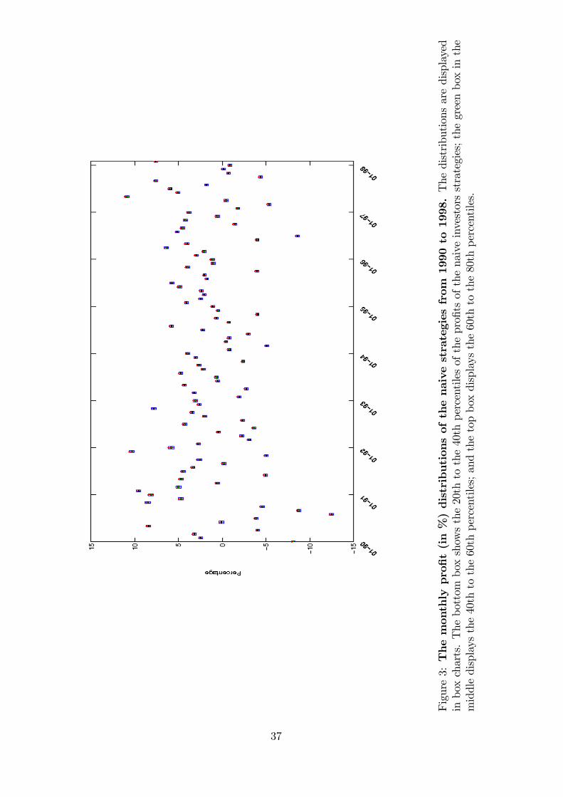
Figure3:Themonthlypro�t(in%)distributionsofthenaivestrategiesfrom

1990

to1998.Thedistributionsaredisplayed

inboxcharts.Thebottom

boxshowsthe20thtothe40thpercentilesofthepro�tsofthenaiveinvestorsstrategies;thegreenboxinthe

middledisplaysthe40thtothe60thpercentiles;andthetopboxdisplaysthe60thtothe80thpercentiles.

37

Figure4:Thecentered

monthlypro�t(in%)distributionsofthenaive

investorsstrategiesfrom

1990

to1998.The

distributionsarecenteredbytheirmediansanddisplayedinboxcharts.Thebottom

boxshowsthe20thtothe40thpercentilesofthe

pro�tsofthenaiveinvestorsstrategies;thegreenboxinthemiddledisplaysthe40thtothe60thpercentiles;andthetopboxdisplaysthe

60thtothe80thpercentiles.

38

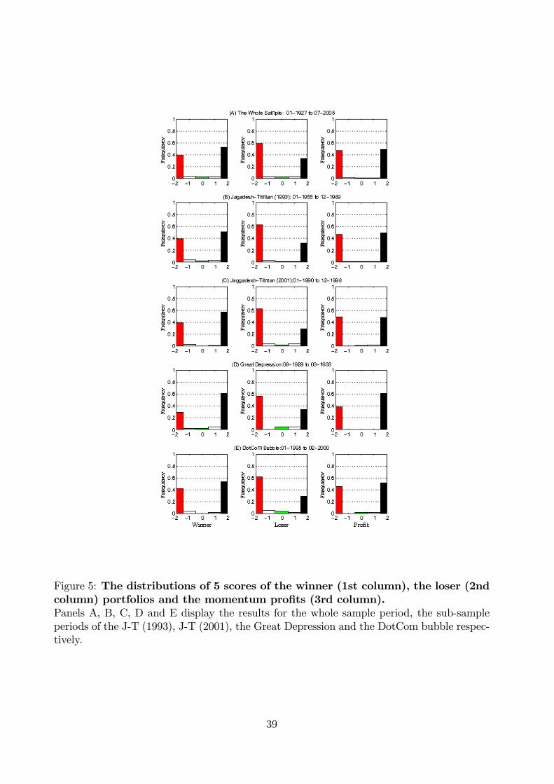
Figure 5: The distributions of 5 scores of the winner (1st column), the loser (2ndcolumn) portfolios and the momentum pro�ts (3rd column).Panels A, B, C, D and E display the results for the whole sample period, the sub-sampleperiods of the J-T (1993), J-T (2001), the Great Depression and the DotCom bubble respec-tively.

39

Figure6:

The

monthly

return

(in

%)

distributions

ofthe

momentum

pro�ts:

JT(2001):

1990-1998.

Thedistributionsaredisplayedinboxcharts.Thebottom

boxshowsthe20thtothe40thpercentilesofthepro�tsofthenaivein-

vestorsstrategies;thegreenboxinthemiddledisplaysthe40thtothe60thpercentiles;andthetopboxdisplaysthe60thtothe80th

percentiles.Thedeviationsofthemomentumpro�tsabovethetop80thpercentileofthepro�tsofthenaivestrategiesareinblue;andthe

deviationsofthemomentumpro�tsbelowthebottom

20thpercentileofthepro�tsofthenaivestrategiesareinred.

40

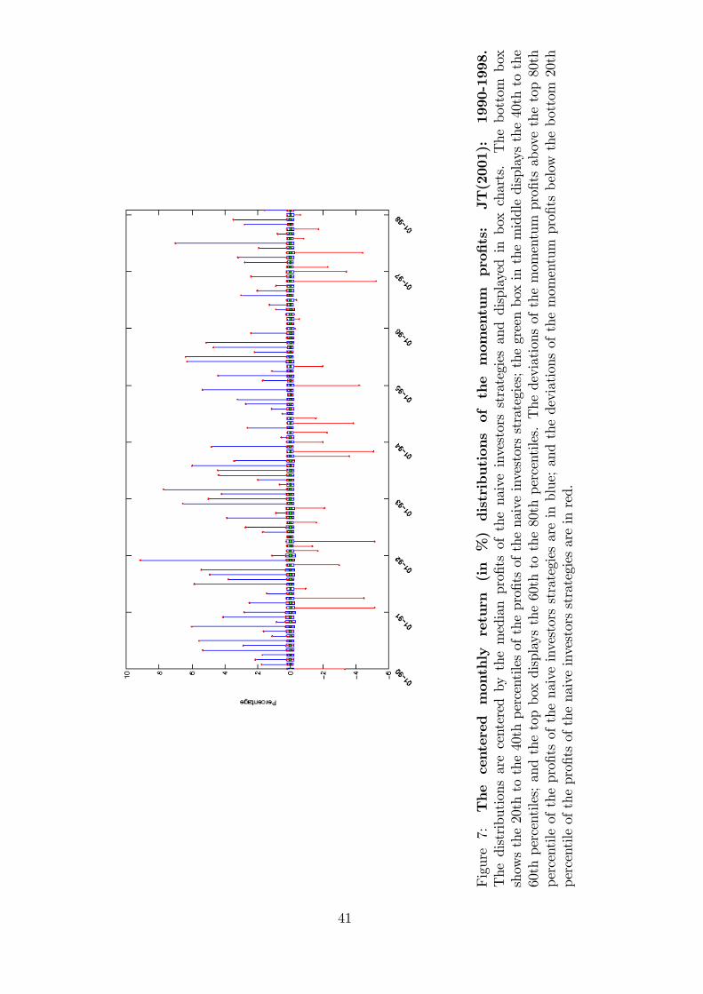
Figure7:

Thecentered

monthly

return

(in%)distributionsof

themomentum

pro�ts:

JT(2001):

1990-1998.

Thedistributionsarecenteredby

themedianpro�tsofthenaiveinvestorsstrategiesanddisplayedinboxcharts.Thebottom

box

showsthe20thtothe40thpercentilesofthepro�tsofthenaiveinvestorsstrategies;thegreenboxinthemiddledisplaysthe40thtothe

60thpercentiles;andthetopboxdisplaysthe60thtothe80thpercentiles.Thedeviationsofthemomentumpro�tsabovethetop80th

percentileofthepro�tsofthenaiveinvestorsstrategiesareinblue;andthedeviationsofthemomentumpro�tsbelowthebottom

20th

percentileofthepro�tsofthenaiveinvestorsstrategiesareinred.

41

Figure 8: The distributions of 11 scores of the winner (1st column), the loser (2ndcolumn) portfolios and the momentum pro�ts (3rd column).Panels A, B, C, D and E display the results for the whole sample period, the sub-sampleperiods of the J-T (1993), J-T (2001), the Great Depression and the DotCom bubble respec-tively.

42

Documents

Informed Momentum Trading versus Uninformed Naive ... · Informed Momentum Trading versus Uninformed "Naive" Investors Strategies Anurag Banerjee and Chi-Hsiou ... For this purpose