Embed Size (px)
Citation preview

InformatIve PsychometrIc fIlters
RobeRt A. M. GReGson

Previous Books by the Author
Psychometrics of SimilarityTime Series in Psychology
Nonlinear Psychophysical Dynamicsn-Dimensional Nonlinear Psychophysics
Cascades and Fields in Perceptual Psychophysics

InformatIve PsychometrIc fIlters
RobeRt A. M. GReGson

Published by ANU E Press The Australian National University Canberra ACT 0200, Australia Email: [email protected] Web: http://epress.anu.edu.au
National Library of Australia Cataloguing-in-Publication entry
Gregson, R. A. M. (Robert Anthony Mills), 1928- . Informative psychometric filters.
Bibliography. Includes index. ISBN 1 920942 65 3 (pbk). ISBN 1 920942 66 1 (online).
1. Psychometrics - Case studies. 2. Human beings - Classification. 3. Psychological tests. 4. Reliability. I. Title.
155.28
All rights reserved. No part of this publication may be reproduced, stored in a retrieval system or transmitted in any form or by any means, electronic, mechanical, photocopying or otherwise, without the prior permission of the publisher.
Cover design by Teresa Prowse. The image on the front cover, that resembles a scorpion, is the Julia set in the complex plane of the Complex Cubic Polynomial used as a core equation in Nonlinear Psychophysics; it is employed in its equation form in some chapters in this book, and is discussed in more detail in the author’s three previous books on nonlinear psychophysics and in some articles in the journal Nonlinear Dynamics, Psychology and Life Sciences
Printed by University Printing Services, ANU
This edition © 2006 ANU E Press

Preface
There has been a time gap in what I have published in monograph form,during which some very important and profound shifts have developed inthe way we can represent and analyse the sorts of data that human organ-isms generate as they progress through their lives. In that gap I have beenfortunate enough to make contact with and exchange ideas with some peo-ple who have chosen to explore nonlinear dynamics, and to see if the ideasthat are either pure mathematics or applications in various disciplinesother than psychology can be usefully explored as filters of behaviouraltime series.
Three strands in my previous published work have come togetherhere; they are time series, psychophysics, and nonlinear nearly chaotic dy-namics. Also, the width in scale of the data examples examined has broad-ened to include some psychophysiological and social processes. There hasevolved a proliferation of indices, hopefully to identify what is happeningin behavioural data, that can be regarded as partial filters of informationwith very varying efficiency.
The title of this effort was selected to emphasise that what is measuredis often information or entropy, and that the focus is on problems and datathat are ill-behaved as compared with what might be found in, say, physicsor engineering or neurophysiology. The object is to model in a selectiveway, to bring out some features of an underlying process that make somesense, and to avoid misidentifying signal as noise or noise as signal.
Recent developments in psychophysiology (Friston, 2005) have em-ployed networks of mixed forward, reverse and lateral processes, some

ii INFORMATIVE PSYCHOMETRIC FILTERS
of which are linear and some nonlinear. That form of construction bringsus closer to neurophysiological cortical structures, and takes theory fur-ther than is pursued here, though there is in both approaches an explicitassumption of nonlinear mappings playing a central role in what is nowcalled the inverse problem; that is to say, working back from input-outputdata to the identification of a most-probable generating process.
There is no general and necessary relationship between identifiabilty,predictability and controllability in processes that we seek to understandas they evolve through time. In the physical sciences sometimes the threeare sufficiently linked that we can model, and from a good fitting modelwe can predict and control. But in many areas we may be able to controlwithout more than very local prediction, or predict without controlling,because the process under study is simple and linear, and autonomousfrom environmental perturbations. That does not hold in the life sciences,particularly in psychology outside the psychophysical laboratory.
The unidentifiabilty or undecidabilty in identification, prediction andcontrol can be expressed in information measures, and in turn, using sym-bolic dynamics, can be expressed theoretically in terms of trajectories ofattractors on manifolds. It is the extension of our ideas from linear autocor-relation and regression models to nonlinear dynamics that has belatedlyimpacted on some areas of psychology explored here.
A related problem that is unresolved in the current literature, for exam-ple in various insighful studies in the journal Neural Computation, is thatof defining complexity. The precise and identifiable differences betweencomplexity and randomness have been a stumbling block for those whowant to advance very general metrics for differentiating the entropy prop-erties of some real data in time-series form. I have not added to that dis-pute here, but sought simply to illustrate what sorts of complicated, non-stationary and locally unpredictable behaviour are ubiquitous in some ar-eas of psychology. The approach is more akin to exploratory data analysisthan to an algebraic formalism, without wishing to disparage either.
The problems of distinguishing between the trajectories of determinis-tic processes and the sequential outputs of stochastic processes, and con-sequently the related problem of identifying the component dynamics of

iii
mixtures of the two types of evolution, has produced a very extensive lit-erature of theory and methods. One method that frequently features is so-called box-counting or cell-mapping, where a closed trajectory is trappedin a series of small contiguous regions as a precursor to computing mea-sures of the dynamics, particularly the fractal dimensionality (for an ex-ample, which has parallels in the analysis of cubic maps in nonlinear psy-chophysics, see Udwadia and Guttalu, 1989).
Serious difficulties are met in identifying underlying dynamical pro-cesses when real data series are relatively short and the stochastic part istreated as noise (Aguirre & Billings, 1995), it is not necessarily the casethat treating noise as additive and linearly superimposed is genericallyvalid (Bethet, Petrossian, Residori, Roman & Fauve, 2003). Though diversemethods are successfully in use in analysing the typical data of some dis-cipines, as in engineering, there are still apparently irresolvable intractabil-ities in exploring the biological sciences (particularly including psychol-ogy), and a proliferation of tentative modifications and computational de-vices have thus been proposed in the current literature.
The theoretical literature is dominated by examples from physics, suchas considerations of quantum chaos, which are not demonstrably relevantfor our purposes here. Special models are also created in economics, butmacroeconomics is theoretically far removed from most viable models inpsychophysiology. Models of individual choice, and the microeconmicsof investor decisions, may have some interest for cognitive science, butthe latter appears to be more fashionably grounded, at present, in neuralnetworks, though again the problem of simultaneous small sample sizes,nonlinearity, non-stationarity, and high noise have been recognised andaddressed (Lawrence, Tsoi & Giles, 1996).
One other important social change in the way sciences exchange in-formation has in the last decade almost overtaken the printed word. Forany one reference that can be cited in hard copy, a score or more are im-mediately identifiable in internet sources such as Google, and the changesand extensions of ideas, and perhaps also their refutation, happens at arate that bypasses the printed text even under revisions and new editions.For this reason, there are some important topics that are not covered here,

iv INFORMATIVE PSYCHOMETRIC FILTERS
tools such as Jensen-Shannon divergence are related to entropy and tometric information and could well be used to augment the treatment ofnonlinear and non-stationary psychological data but so far have not beenconsidered. We urge the reader to augment and criticise the present textby checking developments in the electronic sources, particulary focussingon work such as that by Fuglede and Topsøe (www.math.ku.dk/topsoe/)on Jensen-Shannon divergence, or Nicolis and coworkers (2005) on dy-namical aspects of interaction networks, that have relevance and promise.Jumps between modes of dynamical evolution even within one time se-ries essentially characterise psychological processes, and transient statessuch as chimera (Abrams and Strogatz, 2006) may yet be identified in psy-chophysiology.
I want to thank various people who have encouraged or provoked meto try this filtering approach, and to bring together my more recent workthat is scattered over published and unpublished papers, conference pre-sentations, invited book chapters, and even in book reviews. One very con-genial aspect of the modern developments in applied nonlinear dynam-ics is the conspicuously international character of the activity. ProfessorsStephen Guastello and Fred Abraham in the USA, Hannes Eisler in Swe-den, John Geake in England, Ana Garriga-Trillo in Spain, and Don Byrneand Rachel Heath in Australia, have all offered me constructive help orencouragement over the last decade.
School of PsychologyThe Australian National University

Contents
1 Introduction 1 FiltersandFiltering . . . . . . . . . . . . . . . . . . . . . . . . . . . . . . . . . . . . . . . . . . . . . . . . 7 EventSeries . . . . . . . . . . . . . . . . . . . . . . . . . . . . . . . . . . . . . . . . . . . . . . . . . . . . . . 16 MarkovandHiddenMarkovmodels . . . . . . . . . . . . . . . . . . . . . . . . . . . . . . . . 18 Stimulus-responsesequences . . . . . . . . . . . . . . . . . . . . . . . . . . . . . . . . . . . . . . . 19 LimitsonIdentifiability . . . . . . . . . . . . . . . . . . . . . . . . . . . . . . . . . . . . . . . . . . . . 22 Somepeculiaritiesofpsychophysicaltimeseries . . . . . . . . . . . . . . . . . . . . . . 24 MeasureChains . . . . . . . . . . . . . . . . . . . . . . . . . . . . . . . . . . . . . . . . . . . . . . . . . . 27 OtherSpecialCasesofTransitionMatrices . . . . . . . . . . . . . . . . . . . . . . . . . . . 27
2 Information, Entropy and Transmission 33 Shadowing . . . . . . . . . . . . . . . . . . . . . . . . . . . . . . . . . . . . . . . . . . . . . . . . . . . . . . 36 FittingaModelplusFilter . . . . . . . . . . . . . . . . . . . . . . . . . . . . . . . . . . . . . . . . . 38 PreliminaryDataExamination . . . . . . . . . . . . . . . . . . . . . . . . . . . . . . . . . . . . . . 40 RelaxationofMetricAssumptions . . . . . . . . . . . . . . . . . . . . . . . . . . . . . . . . . . 41 Fast/SlowDynamics . . . . . . . . . . . . . . . . . . . . . . . . . . . . . . . . . . . . . . . . . . . . . . 45 FilteringSequentialDynamics . . . . . . . . . . . . . . . . . . . . . . . . . . . . . . . . . . . . . 49
3 Transients onto Attractors 53 Manifolds . . . . . . . . . . . . . . . . . . . . . . . . . . . . . . . . . . . . . . . . . . . . . . . . . . . . . . . . 56 Identificationoflocalmanifoldregions . . . . . . . . . . . . . . . . . . . . . . . . . . . . . . 57 TreatingasTimeSeries . . . . . . . . . . . . . . . . . . . . . . . . . . . . . . . . . . . . . . . . . . . . 60 TremorSeries . . . . . . . . . . . . . . . . . . . . . . . . . . . . . . . . . . . . . . . . . . . . . . . . . . . . 62 Higher-orderDynamics . . . . . . . . . . . . . . . . . . . . . . . . . . . . . . . . . . . . . . . . . . . 68

InformatIve PsychometrIc fIltersvi
4 Inter- and Intra-level Dynamics of Models 71 Intermittencies . . . . . . . . . . . . . . . . . . . . . . . . . . . . . . . . . . . . . . . . . . . . . . . . . . . 78 SynchronyandBinding . . . . . . . . . . . . . . . . . . . . . . . . . . . . . . . . . . . . . . . . . . . . 83 BoundedCascadesin6-dpartitionedNPD . . . . . . . . . . . . . . . . . . . . . . . . . . . 85 ComparisonControlConditionsfortheDynamics . . . . . . . . . . . . . . . . . . . . 92 SerialHypercycling . . . . . . . . . . . . . . . . . . . . . . . . . . . . . . . . . . . . . . . . . . . . . . . 94 Theextensionto2Dand3DLattices . . . . . . . . . . . . . . . . . . . . . . . . . . . . . . . . . 95 Conclusions . . . . . . . . . . . . . . . . . . . . . . . . . . . . . . . . . . . . . . . . . . . . . . . . . . . . . 100 Appendix1 . . . . . . . . . . . . . . . . . . . . . . . . . . . . . . . . . . . . . . . . . . . . . . . . . . . . . 101 Appendix2 . . . . . . . . . . . . . . . . . . . . . . . . . . . . . . . . . . . . . . . . . . . . . . . . . . . . . 103
5 A Bivariate Entropic Analogue of the Schwarzian Derivative 105 TheSchwarzianderivative . . . . . . . . . . . . . . . . . . . . . . . . . . . . . . . . . . . . . . . . 108 CoarseEntropyFiltering . . . . . . . . . . . . . . . . . . . . . . . . . . . . . . . . . . . . . . . . . . 109 ASchwarzianderivativeanalogue . . . . . . . . . . . . . . . . . . . . . . . . . . . . . . . . . .111 Extendingtothebivariatecase . . . . . . . . . . . . . . . . . . . . . . . . . . . . . . . . . . . . .114 ThemanifoldofthelaggedBESf . . . . . . . . . . . . . . . . . . . . . . . . . . . . . . . . . . . 120 Discussion . . . . . . . . . . . . . . . . . . . . . . . . . . . . . . . . . . . . . . . . . . . . . . . . . . . . . . 121 Appendix:BernsteineconomicdataandPhysionetdata . . . . . . . . . . . . . . 125
6 Tribonacci and Long Memory 129 TheTribonacciSeries . . . . . . . . . . . . . . . . . . . . . . . . . . . . . . . . . . . . . . . . . . . . . 132 Higher-OrderDerivedSeries . . . . . . . . . . . . . . . . . . . . . . . . . . . . . . . . . . . . . . 137 Discussion . . . . . . . . . . . . . . . . . . . . . . . . . . . . . . . . . . . . . . . . . . . . . . . . . . . . . . 140 ClassicalARMAanalyses . . . . . . . . . . . . . . . . . . . . . . . . . . . . . . . . . . . . . . . . . 144 ApEnmodelling . . . . . . . . . . . . . . . . . . . . . . . . . . . . . . . . . . . . . . . . . . . . . . . . . 145 ESfAnalyses . . . . . . . . . . . . . . . . . . . . . . . . . . . . . . . . . . . . . . . . . . . . . . . . . . . . 148 ClassicalARMAanalyses . . . . . . . . . . . . . . . . . . . . . . . . . . . . . . . . . . . . . . . . . 149 Discussion . . . . . . . . . . . . . . . . . . . . . . . . . . . . . . . . . . . . . . . . . . . . . . . . . . . . . . 152 HumanPredictiveCapacities . . . . . . . . . . . . . . . . . . . . . . . . . . . . . . . . . . . . . . 158 Conclusions . . . . . . . . . . . . . . . . . . . . . . . . . . . . . . . . . . . . . . . . . . . . . . . . . . . . . 163 Note . . . . . . . . . . . . . . . . . . . . . . . . . . . . . . . . . . . . . . . . . . . . . . . . . . . . . . . . . . . 164 PostscriptontheFigures . . . . . . . . . . . . . . . . . . . . . . . . . . . . . . . . . . . . . . . . . . 173

vii
7 Rescorla’s Theory of Conditioning 175 ExtensiontoDiscriminationLearning . . . . . . . . . . . . . . . . . . . . . . . . . . . . . . 177 StructuralAnalogies . . . . . . . . . . . . . . . . . . . . . . . . . . . . . . . . . . . . . . . . . . . . . 178 Simulationin2DNPD . . . . . . . . . . . . . . . . . . . . . . . . . . . . . . . . . . . . . . . . . . . . 182 HigherandIndeterminateDimensionality . . . . . . . . . . . . . . . . . . . . . . . . . . 186
8 Nonlinearity, Nonstationarity and Concatenation 189 StatisticalMethods . . . . . . . . . . . . . . . . . . . . . . . . . . . . . . . . . . . . . . . . . . . . . . . 191 TheTimeSeriesUsed . . . . . . . . . . . . . . . . . . . . . . . . . . . . . . . . . . . . . . . . . . . . . 195 ComparisonofHigher-orderAnalyses . . . . . . . . . . . . . . . . . . . . . . . . . . . . . . 201 Discussion . . . . . . . . . . . . . . . . . . . . . . . . . . . . . . . . . . . . . . . . . . . . . . . . . . . . . . 205 Notes . . . . . . . . . . . . . . . . . . . . . . . . . . . . . . . . . . . . . . . . . . . . . . . . . . . . . . . . . . 207
9 Time Series of Disasters 215 LimitsonIdentifiability . . . . . . . . . . . . . . . . . . . . . . . . . . . . . . . . . . . . . . . . . . . 217 TheDeathsSeries,x . . . . . . . . . . . . . . . . . . . . . . . . . . . . . . . . . . . . . . . . . . . . . . 220 TheTimeIntervalsSeries,y . . . . . . . . . . . . . . . . . . . . . . . . . . . . . . . . . . . . . . . 221 TheLocalDeathRatesSeries,z . . . . . . . . . . . . . . . . . . . . . . . . . . . . . . . . . . . . 222 Discussion . . . . . . . . . . . . . . . . . . . . . . . . . . . . . . . . . . . . . . . . . . . . . . . . . . . . . . 227 SeriesofIrrationalBeliefs . . . . . . . . . . . . . . . . . . . . . . . . . . . . . . . . . . . . . . . . . 230
10 Perron-Frobenius at the Edge of Chaos 237 ALeakyBistableMatrix . . . . . . . . . . . . . . . . . . . . . . . . . . . . . . . . . . . . . . . . . . 239 Probabilitypartitioning . . . . . . . . . . . . . . . . . . . . . . . . . . . . . . . . . . . . . . . . . . . 239 ATremorSeries . . . . . . . . . . . . . . . . . . . . . . . . . . . . . . . . . . . . . . . . . . . . . . . . . . 240 Informationmeasuresasnon-stationarityindices . . . . . . . . . . . . . . . . . . . . 245 Discussion . . . . . . . . . . . . . . . . . . . . . . . . . . . . . . . . . . . . . . . . . . . . . . . . . . . . . . 249 DynamicsofCardiacPsychophysiology . . . . . . . . . . . . . . . . . . . . . . . . . . . . 250 HigherOrderStatistics,bESf . . . . . . . . . . . . . . . . . . . . . . . . . . . . . . . . . . . . . . 255 SubdividingtheThirdEpoch . . . . . . . . . . . . . . . . . . . . . . . . . . . . . . . . . . . . . . 256 Self-SimilarityatDifferentScales . . . . . . . . . . . . . . . . . . . . . . . . . . . . . . . . . . . 258 Multipleanalysesonsampleseries . . . . . . . . . . . . . . . . . . . . . . . . . . . . . . . . . 259 PanicPre-dynamics . . . . . . . . . . . . . . . . . . . . . . . . . . . . . . . . . . . . . . . . . . . . . . 263

InformatIve PsychometrIc fIltersviii
Notes . . . . . . . . . . . . . . . . . . . . . . . . . . . . . . . . . . . . . . . . . . . . . . . . . . . . . . . . . . 266 Appendix . . . . . . . . . . . . . . . . . . . . . . . . . . . . . . . . . . . . . . . . . . . . . . . . . . . . . . . 267
11 Appendix: Nonlinear Psychophysical Dynamics 269
References and Bibliography 279
Subject Index 307

Chapter 1
Introduction
The reader should be warned against being seduced into think-ing that linearization tells the whole story.
(Infeld and Rowlands, 2000, p. 296)
This monograph is about building models of psychological or psy-chophysiological data that extend through time, are inherently unstableand, even from the perspective of the applied mathematician, are often in-tractable. Such instabilities have not gone unnoticed by statisticians andeven such patterns as good and bad patches in the performance of sportsteams, which are inexplicable to some of their followers, have been mod-elled. Attempts to address this problem in a diversity of disciplines are le-gion and it is only data of interest to the psychologist and the constructorof psychological measurements that are our focus. This does not mean thatnew methods will not emerge, even while this monograph is being writ-ten. Strange attractors and soliton metamorphoses have been added to therange of theoretical constructs available to the physicist and the sorts ofdata that we may meet in psychometrics are often appropriately treated asevidence of non-coherence, though that term is, as yet, rarely used outsidephysics (Infeld and Rowlands, 2000). In one sense, psychological data canbe even worse because they jump about in their dynamics or are induced

2 INFORMATIVE PSYCHOMETRIC FILTERS
to do so by the action of the environment providing stimuli. One mightthink of any attempt at modelling a real life process extending throughtime as a compromise between plausibility of a representation of substan-tive data and mathematical tractability. If that were so, it could be a zerosum game in which one is achieved at the expense of the other. But it isnot. There can be and frequently is loss on both sides of the compromise.
Historically, we could go back to 1812, when one of the first seriousmathematical models of sensory or cognitive processes was created byHerbart (translated by Gregson, 1998). He had the profound insight that
The calculation of the rises and falls of imagery in conscious-ness this most general of all psychological phenomena, ofwhich all others are all only modifications would only requirea quite simple algebraic representation, if the imagery couldbe said to be directly proportional in all its strength, if not ithas its origins in the perception of time itself, and would showagainst already existing contrasts.
But that does little more than remind us that the subsequent evolution ofthe discipline was a history of false starts and neglected solutions. Thereare two sorts of mathematical borrowing that are found in the history ofquantitative psychology: borrowing of a wide area of mathematically ex-pressed theory already in use in physics, biology or engineering, such asstochastic differential equations, or catastrophe theory; and borrowing ofspecific equations that were originally advanced as models in some sub-stantive area that has no immediate intuitive parallels with psychology.The first sort of borrowing, if it can be called borrowing, is involved hereand has been one of increasing interest recently as symbolic dynamics(Jimenez-Montano, Feistel and Diez-Martinez, 2004). The second sort goesback a long way; for example, it seems not to be generally known that theuse of a linear model with an added Gaussian random residual compo-nent, introduced by Fechner in the 1850s, goes back, via Weber, to Gaussand the resurveying of the streets of Hannover after the Napoleonic warsand to Gauss’s monograph on least squares of 1809 (Buhler, 1986).

INTRODUCTION 3
It seems to be relatively rare for mathematical psychology to produceits own equations that are not copies of something in physics or biology,such as borrowing the logistic equation created for population dynamics,but that may be an unfair criticism. If hard work has already been done,one can build on it. The complex cubic Gamma recursion of nonlinear psy-chophysics (Gregson, 1988, 1992), will be quoted later. It resembles someother mathematical models but is a bit different; a model can be one of afamily and, at the same, uniquely applicable to some substantive area ofscience.
The title of this monograph was chosen to include the word infor-mative, which has a special meaning that will characterise the approachtaken: informative implies information, and information implies informa-tion theory and its extensions, associated with the names Kullback, Leiblerand Akaike (de Leeuw, 1992). The use of information theory in psychol-ogy had a brief popularity, due in part to the efforts of Attneave (1959),preceding methods, in the later 20th century, that have had some partialimpact on psychometrics but rather more on engineering. Recently, in-formation measures as a basis of choice between alternative models hasbeen strongly advocated in biology (Burnham and Anderson, 2002). Thisis an approach with which we have strong sympathy, but one that sets usat odds with some preferred traditions in psychophysics and in appliedstatistics. Much of both classical and modern psychophysics is written out-side time. It is not an area of dynamics, let alone nonlinear dynamics, butone of steady-state stimulus-response mapping (Falmagne, 2002). Therehave been important attempts to extend this dynamically: Helson’s (1964)work on adaptation level theory was one, and Vickers (1979) on accumu-lator theory was another. Trying to build time series analysis into the to-tal picture that was mostly linear theory created this author’s 1983 workTime Series in Psychology. But what has happened since creates a need fora fundamental rethink if nonlinear systems are to play a important role.
Ignoring sequential effects in stimulus-response mappings by only ex-amining behaviour under asymptotic steady-state conditions is useful ifsome sorts of individual differences in responses to the environment areimportant; the logic of a simple intelligence or memory test does not ask

4 INFORMATIVE PSYCHOMETRIC FILTERS
how a respondent got, over some years, to be what he or she now is,but what he or she can now do when faced with tasks of various diffi-culties. One cannot investigate absolutely everything at once and delib-erately choosing not to ask some questions is, perhaps paradoxically, oneof the bases of scientific method. But asking too many questions at once,that is, collecting a host of data on all potentially relevant variables, cancreate studies in which nothing is identifiable or decidable. In statistics,this is called the problem of overdetermination or lack of degrees of free-dom. The counter argument, particularly in nonlinear systems, is that, ifvariables are taken one by one and not in clusters as they occur in thereal world, then the nature of their interaction is obscured and causality isobliterated.
————————————————-Figure 1.1
EVENT Ef(E)−→ Receptors R
f(E,R)−→ NEURALyφ ACTIVITY Ny ySampling g(E) −→ Sensory S1yφ ψφO
yψφ(N,S1)
INSTRUMENTF (g(E))−→ Sensory S2
φψ(g(E))−→ OBSERVER
−ATION
————————————————-
There are a number of locations in Figure 1.1 where a psychophysi-cal mapping may be created. Indeed, in the 1860s, Fechner distinguisedwhat he called psychophysics from below and psychophysics from above.In the 1890s, Wundt wrote as though he was predominantly seeing him-self as doing physiology. It is explicit in Fechner (1860), that he wished

INTRODUCTION 5
to bring together evidence in one framework from all of physics, phys-iology and everyday life. There are two pathways in Figure 1.1 that areof interest: from the Event, through S1, to the Observer; and through theIntrumentation of the Event and S2 to the Observer. The path through S2is, as drawn, a bit of a cheat, as it should really go from Instrumentationback to Receptors R and then via S1. The path via S2 is drawn to empha-sise that some Events are never directly available to our senses, such asvoltages or radio waves (except in some pathologies, apparently), but wecan and do read pointer readings and may consider the psychophysicalrelations between pointer readings and our awareness of events in waysthat were never available in the mid-19th century. Yesterday, as I am writ-ing this, it was hot and muggy, so I consulted the barometer hanging inthe hallway of my home, and read humidity and temperature dials. Yes,I was right. It was information consistent with feeling hot and stuffy; itwasn’t an illusion due to me having a bad cold. But I did not have a soundmeter handy to check the loudness of my hi-fi system. That just soundedagreeable, though the nearby thunderstorm sounded threatening.
But there is an immediate complication: a step labelled ’sampling’ in-dicates that only parts of the Event get represented in the Instrumentationand some of the properties encoded may never correspond to our sen-sory experiences. This is particularly true for detailed chemical analyses,as compared with odours and tastes. Unprocessed signals can come as faras S1 and/or S2, but get no further.
The psychophysical mappings, symbolised in Figure 1.1 as ψφ terms,and expressed in equations; traditionally they are usually called laws,named after Weber, Fechner, or Plateau (but his was later reinstated byStevens). These equations are peculiar, for two reasons: they are usually in-completely expressed, as they have no stipulated boundary conditions butare intended only to hold within a limited Event amplitude range, calledlower and upper thresholds; and they treat the Event as fixed in time, suf-ficiently encoded as a scalar variable. There is no provision for dynamicsin the environment, but some for delays in the sensory pathways. Fechnerregarded the method of average response to a fixed stimulus as one for get-ting a best estimate from repeated presentations of a fixed environmental

6 INFORMATIVE PSYCHOMETRIC FILTERS
stimulus that created local second-order variability in the sensory system,though the dynamics of neither were then of interest, only the first andsecond moments. Much of contemporary psychophysics does just that.
If one wanted to rewrite Fechner’s version of Weber’s law with bound-aries, then for Response = ψ, Stimulus = φ,
f(∆1φ|p = .5) = a · log(φ), φmin < φ < φmax [1.1]
might be acceptable. Note that the equation is strictly not psychophysical,in that psychological units of magnitude are replaced by a j.n.d. operationexpressed in physical units. There are serious problems with the rigorousinterpretation of [1.1] as a scale of measurement, that are discussed byLuce and Galanter (1951).
The alternative popularised by Stevens (1951) is
ψ = a · φb, φmin < φ < φmax [1.2]
and this form does map from physical to psychological measures, but thechoice of what actually to use as ψ is very arbitrary.
As both [1.1] and [1.2] are monotonic and, as written, have no addi-tive constants, one can be transformed to the other. There are objections to[1.2] concerning what happens in the region near φmin. Those objectionsgo back to Wundt. In order for an observer to perform the tasks necessaryto create data for either equation, some sort of comparison of successiveevents is needed, but the events are taken as being independent realisa-tions of the same stationary process. To put it another way, they are bothmodels of relative judgement or, as Luce and Galanter subsumed it, in thegeneral category of discrimination tasks. What is also interesting here isthat neither equation describes a process that is self-terminating in time,whereas in nonlinear dynamics that can be done without adding indepen-dent boundary conditions. What are treated as events are not themselvesinstantaneous, but the temporal extension of the events may not featurein [1.1] or [1.2], unless the event is itself a time interval whose durationis to be judged. The time to process in S1 or S2 may be much longer thanthe temporal duration of the event, as is involved in short-term memory,

INTRODUCTION 7
or the delays in the instrumentation and it is this difference in processingduration that commonly characterises the whole system. A consequenceis that separate equations for response latencies, or reaction times as theywere sometimes called, have to be added to the system. A special case thatarises in audition is the perception of pitch; the signal is fluctuating in timeand the eventual response is a single unfluctuating level, the Neural Net-work in the ear integrates the fluctuations in a time sample, so the eventmust have duration. We will explore these filters in later chapters.
The pathways in Figure 1.1 can be thought of as imperfect informa-tion transmitters in various senses: the instrumentation only detects someEvent properties, both intentionally and unintentionally; the neural net-works that include sensory channels to the brain have limitations in activ-ity level capacities and rates of transmission; and the eventual consciousobserver has fluctuations in attention and memory, both short and longterm.
Filters and Filtering
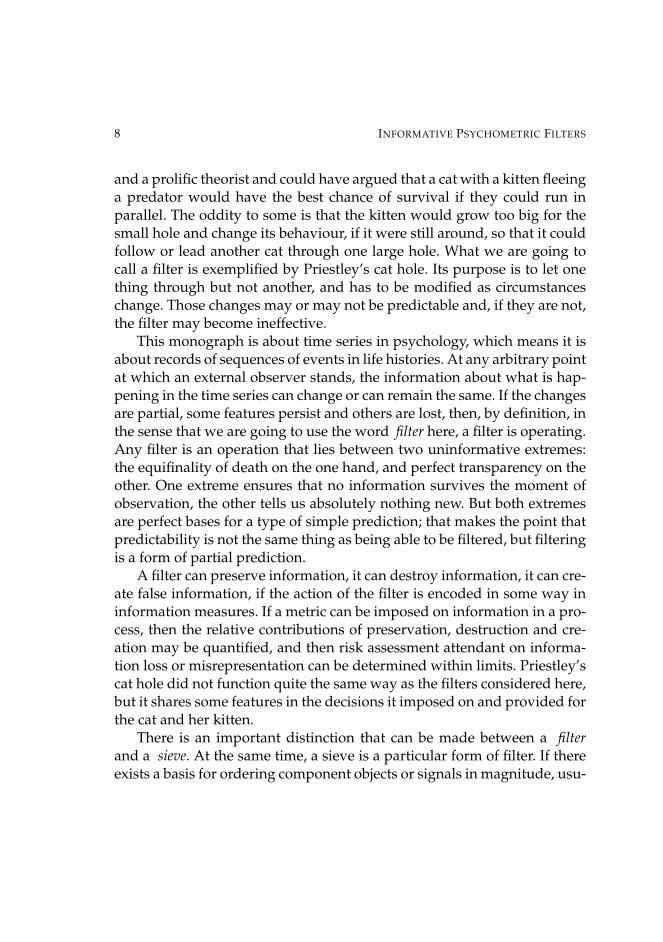
There is a story, probably not apocryphal, that the great British chemistJoseph Priestley (1733-1804) cut a hole in the base of his door so that hiscat could come and go through it1. This in itself is not exceptional, todaypeople do it with a little hinged panel on the hole and it is called a cat-flap.But Priestley also cut, alongside the larger hole that was big enough for anadult cat but too small for a dog, a much smaller hole for a kitten. This isseen as eccentricity, but can also be the result of shrewd observation of catbehaviour: a mother cat will carry a very small kitten by holding the backof the kitten’s neck in her jaws, older kittens who can see and run will runalongside their mother where she can keep an eye on them, not necessarilyfollow her from behind, out of her sight. Priestley was a careful observer
1 This story is also attributed to Sir Isaac Newton, who is said to have cut not one holefor one kitten but four holes alongside each other, for the whole litter. The principle ofthe story is unaltered but, as recent scholarship portrays Priestley as a nicer person thanNewton, let us give him some credit.
8 INFORMATIVE PSYCHOMETRIC FILTERS
and a prolific theorist and could have argued that a cat with a kitten fleeinga predator would have the best chance of survival if they could run inparallel. The oddity to some is that the kitten would grow too big for thesmall hole and change its behaviour, if it were still around, so that it couldfollow or lead another cat through one large hole. What we are going tocall a filter is exemplified by Priestley’s cat hole. Its purpose is to let onething through but not another, and has to be modified as circumstanceschange. Those changes may or may not be predictable and, if they are not,the filter may become ineffective.
This monograph is about time series in psychology, which means it isabout records of sequences of events in life histories. At any arbitrary pointat which an external observer stands, the information about what is hap-pening in the time series can change or can remain the same. If the changesare partial, some features persist and others are lost, then, by definition, inthe sense that we are going to use the word filter here, a filter is operating.Any filter is an operation that lies between two uninformative extremes:the equifinality of death on the one hand, and perfect transparency on theother. One extreme ensures that no information survives the moment ofobservation, the other tells us absolutely nothing new. But both extremesare perfect bases for a type of simple prediction; that makes the point thatpredictability is not the same thing as being able to be filtered, but filteringis a form of partial prediction.
A filter can preserve information, it can destroy information, it can cre-ate false information, if the action of the filter is encoded in some way ininformation measures. If a metric can be imposed on information in a pro-cess, then the relative contributions of preservation, destruction and cre-ation may be quantified, and then risk assessment attendant on informa-tion loss or misrepresentation can be determined within limits. Priestley’scat hole did not function quite the same way as the filters considered here,but it shares some features in the decisions it imposed on and provided forthe cat and her kitten.
There is an important distinction that can be made between a filterand a sieve. At the same time, a sieve is a particular form of filter. If thereexists a basis for ordering component objects or signals in magnitude, usu-

INTRODUCTION 9
ally but not necessarily on a single continuum, then those magnitudes arethe basis on which a sieve separates the set of objects into two or moresubsets and allows one to pass through in time. The idea of a sieve in aphysical sense is thousands of years old, wheat is separated from chaff,gold is panned by swirling out less dense particles from sand or gravel.But when information in time series is being transmitted, it is usual towrite of band pass filtering, a term that covers a diversity of possibilities.Then, events that lie in a narrow magnitude band are given a special sta-tus, either for acceptance or rejection. The bands are often defined in termsof frequency components, as is common practice in electroencephalogramanalyses. What is not passed on may be defined as noise. If very slowly orvery quickly fluctuating components in a mixture of components of a timeseries are given a priori some special meaning, then they are filtered in orout by using, respectively, high- or low-pass filters. The following diagram(Figure 1.2) is a simple heuristic to relate some parts of filtering.
There is another sense in which information is filtered: censoring. Thename obviously derives from its older usage in distasteful politics or gov-ernment, but has been borrowed by statisticians to indicate when a fre-quency distribution of data has been in some way truncated or trimmed,usually to exclude a long tail or outliers. This obviously implies that thereis some prior notion of what the full frequency distribution would belike and, as a consequence of censorship, estimates of parameters are sus-pected or known to be biased.
The flow diagram in Figure 1.2 is skeletal, it includes most of the in-formation flows that will concern us and where they are but, as it stands,would be useless in exploring any real situation, because it has no equa-tions, variables, parameters, or gains at any point and no specified delaysin the pathways. All these are necessary in order to create a simulation andcompare that simulation against real world events.
The words IN and OUT indicate places where the system would beexternally observable. Externally refers to any instrumentation, either be-havioural or psychophysiological, that is accessible independently of theassumptions in the system representation. A symbol δ indicates variabledelay in feedback (fb) that is controlled independently of the intrinsic de-

10 INFORMATIVE PSYCHOMETRIC FILTERS
————————————————-Figure 1.2
Model
F irst
IN V ersion Noise−→ OUTy y
Time Series Data −→ FILTER −→ Information← fby x y xyOUT New Filter Predictionx
Stationaryx yOUT
xSubset −→ Tests ←− Disparities
xδxIN yOUT
xIterated
y xModel −→ Control−→ fb
InRealT ime
————————————————-
lays of the filtering operations themselves.Many of the steps in the flow diagram are, to some extent, discretionary
and involve decisions about when to stop an iterative revision of mod-elling and prediction. Such iterative processes that should converge, if theanalysis is stable, but might not converge on a useful solution (hence theword ”applicable” is implicit in the title of this monograph), are them-selves the subject of computational filtering when they become written as

INTRODUCTION 11
computer programs. One discretionary step is the abstraction of a subsetof data that, on inspection, appears to be stationary with respect to thelower-order variables of the model being used as the central filter. Lower-order here means the parts of a model that are treated as constant locally intime, so in turn implies taking short subsamples. As always, the problemof non-stationarity is ubiquitous in psychological data.
It is assumed in the flow diagram that the input data that is externallyobservable is complete in terms of the inbuilt assumptions of the initialmodel. However, many data sets are censored, and particularly may bealiased. This term refers to yet another sort of filtering and is most oftenused to denote a situation where high frequency components of a seriesencoded in the frequency domain are lost because the frequency of dis-crete encoding is less than twice the maximum frequency of the signal’scomponents. But aliasing can also arise in a different way; for example, thestatistics of the long series of major accidents resulting in deaths in Englishcoal mines over the century beginning around 1850 does not include acci-dents where there were fewer than 10 men killed at once. Aliasing smallaccidents seriously biases both the distributions of accident magnitudesand the inter-accident intervals in time. This confounds our understand-ing of the relevant causalities. There is no difficulty in imagining similarproblems in self-report records or recall by human subjects who keep di-aries of their misfortunes, moods, or illnesses.
The filtering that yields both information and noise is, in experimen-tal psychology, most commonly that created by the General Linear Model(GLM), of which ANOVA is a special case. The part that is filtered outas noise is assumed to be Gaussian, to have independent identically dis-tributed (i.i.d.) realisations and be independent of the linear model compo-nents. In general, these are empirically false but mathematically tractableassumptions. The GLM is not usually applied iteratively in experimentalpsychology. The assumptions made in the GLM will not be used here, witha few exceptions.
A partitioning between signal and noise is traditional in linear modelsunder stationarity, but it does not follow that analyses in the frequency do-main, when cyclic patterns are observed or suspected, are necessarily most

12 INFORMATIVE PSYCHOMETRIC FILTERS
advantageous. An interesting example of using eigenvector decomposi-tions of autocovariance matrices was described by Basilevsky and Hum(1977); it has various advantages if the time series variables have somemetric properties and can be used for weak stationary short series. It alsohas the advantage that series need not be detrended prior to analysis andthe partitioning of causal components can be easier to interpret. For thesereasons, we will return to eigenvalue methods in some cases in later chap-ters, even though we will need to relax assumptions about metric variablesand stationarity.
The input time series may be multivariate and the measures that com-prise it may be real or complex if they are apparently numerical but, moregenerally, are symbols, encoding different types of behaviour such as areused by ethologists in studying animal behaviour patterns and sequences.Priestley’s cat and her kittens need representation in a series of behavioursequences, parallel in time and space, and assumptions of interdepen-dence of component series can be erroneously filtered out. Non-numericalsymbols are still information and can still be filtered, though the filteringmay then not be possible in the frequency domain. If the initial modelmakes wrong assumptions about the properties of the input series, thenthe filter will not be optimal, as the filter is an extension of the model, builton the same assumptions about the nature of the input. A multicompo-nent time series may be misidentified and wrongly filtered if assumptionsabout the mutual independence of parallel input component channels arewrong.
Special cases, that arise in nonlinear dynamics, where the input seriesis treated as a trajectory in a dynamical system, may also be modelled asrecursive steps within a neural network. In such cases, the variables canbe complex (Hirose, 2003).
Given the suspected existence of a dynamic system in the real world,it is possible to proceed through a series of ordered stages, with successor failure at any stage. Any step may be partially implemented, and thedegree of partial implementation can be sufficient to progress to the nextstage, with a consequent increasing risk of failure.
It is also possible to achieve some later stage, such as Control, without,

INTRODUCTION 13
in fact, having any predictive capacity beyond the short-term.
[1] ObservationThis refers to ordinary language observations of events and properties
of events with minimal theoretical presuppositions. Let us call these theset Ω. One might call this stage extreme atheoretical empiricism.
[2] DescriptionIt is assumed that some framework or vocabulary for grouping and
ordering events is employed, which takes some account, not necessar-ily valid, of the relative substantive a priori significance (not necessarilystatistical significance) and reliability of different data components, whenthey are potentially to be incorporated in a total description of the situationunder examination. The descriptive attributes imposed by the observer arethe set a, b, c, d, ... and so Ω becomes Ωabcd....
[3] MeasurementThis is defined as the first stage in which observations are replaced by
numerical or symbolic encodings, as those numbers x, y, .., with assumedmetric properties of some type µ(x, y, ..), are then the working basis of thenext stages. This is the step at which ordinary language meanings cease tofeature if the encoding is consistent and unambiguous. This consistencyrefers to the mappings Ωabcd... 7→ µ(xy..). In general the mapping will bemany-to-one, multiple instances of events classified as identical in terms oftheir attributes will map into one set of numerical variables. This impliesa condensation of structure prior to formal modelling.
[4] ModellingThis is defined as the formal construction of mathematical or symbolic
programming structures, which are comprised of parameters and vari-ables and the relations between them. This definition is deliberately vague,as it covers any model that can be written as code, in digital or analoguemode, and would thus include any differential-difference equations andrecursive maps. The purpose here is to focus on models that are intended

14 INFORMATIVE PSYCHOMETRIC FILTERS
to reflect the putative properties of system dynamics. If the set of relationaloperators in a model M is ρM, then
M ≡def ρM ,Ωabcd..
[5] IdentificationWhen, by some incomplete process of matching a subsetQ of the prop-
erties of M is matched down to a residual error limit ε with a real data setnot used in [4], the process is said to be Q, ε-identified. This idea parallelsthe statistician’s notions of goodness-of-fit and the costs of misidentifica-tion.
[6] PredictionA prediction is a statement at Q, ε level about a set of events [1] or [2]
that have not been employed in the construction ofM . They may be futureevents, or ones that are already on file but not employed in [4,5].
[7] ControlIn order to write about control it is necessary to define first the notion
of acceptable limits of variation within a Q, ε system. We assume that arepresentation M exists and that it can, over time, drift out of satisfyingQ, ε conditions for M . To control effectively is to add a set of rules for thetransient implementation of a feedback loop that was not originally partof M ; either current variable values are changed by being overwritten, orparameters are reset. If the control is recursive, then the need for predictionis minimal. Otherwise, local predictability is required. Control involvesthe use of energy and thus may reduce the efficiency of a system whichembodies M .
[8] ResponseAll of [1] through [4] may be incomplete and lead to pseudo-
identification in [5]. Importantly, in [1], if we are to consider dynamics,then already observations are tagged as occurring in time and in temporalseparation, coincident or sequential. By Response [8] is meant the capacity

INTRODUCTION 15
of the observer to take protective or corrective action to change the out-comes of the action of a system that cannot be controlled. For example, theweather can be predicted in the very short term, not be well predicted inmedium term, and be well predicted on average with seasonal correctionin the long term. The response is sometimes to carry an umbrella or to usea sun-screen cream.
The change from [1] to [2] involves the use of some categorisation ofraw data, so a priori notions of similarity and difference and clustering be-come involved. When the partially described data are quantified, either bydirect measurement of properties in extension, or by probabilities of classmembership, then we move to [3]. Modelling [4] uses [3] and operations ofidentity and relations. The errors arise at this stage either because of wrongvariables being included at [2,3] or wrong relationships being postulatedin [4]. Dynamic models involve relationships that evolve in time.
All psychological data are samples from the evolving life histories ofthe observed individuals who are the subjects of observation and theoris-ing. From the perspectives of time series analysis they generate data whosenumerical properties are ill-behaved or even ill-defined, and in terms oflinear models they are non-stationary unless some ruthless data smooth-ing or filtering is applied locally. The wider the windows in time throughwhich we observe the behaviour, the more insight we potentially obtain,but the less tractable the data become. Predictability means extrapolationinto future time of dynamic sequences whose structures are incompletelyobserved, and whose instabilities can be shown to be only second-order.
Time series fall into different types: event series, time-interval series,and events-in-time series. Further subdivision of these types is possible,according to whether or not the variables are continuous or categorical,and whether the observed events are treated as seen through narrow win-dows opened upon an underlying continuous process (Krut’ko, 1969) orare assumed to be discrete events exhaustively recorded. The statisticalmethods used to identify sequential dependencies in the dynamics can bequite different for the various types.
Any series which is representable in the time domain can also have anequivalent representation in the frequency domain using Fourier analysis

16 INFORMATIVE PSYCHOMETRIC FILTERS
and, computationally, the Fast Fourier Transform. That approach yields arepresentation of the relative energy in any frequency component of theprocess and is used widely in EEG analyses, which are typically eventseries of potential levels recorded at 3 msec intervals, when a physiologicalsignificance is given to energy in the 10-12 Hz spectral band.
Event Series
An event series is here defined as a series of events equally spaced in time.Event xj arrives at time τj , but the temporal units in which τ is recordedplay no part in the data analysis, though they play a part in the subsequentinterpretation of the process. The first differences of the time process ∆1τjare zero or taken as constant, or are assumed to be sufficiently near con-stant not to be important in their variation. For example, observations aremade once a month on total suicides in a community, or once every ten sec-onds on attention shifts to a television program, or once every ten msecsto an EEG measure. The time series analysis is applied to the sequence,
x1, ..., xj , ...., xn
which is taken to be unbroken, though missing values which are randomlydistributed and do not exceed more than about 5% of n can be filled by lo-cal linear interpolation, matching iteratively the first two moments of thedistribution of x. The widespread use of ARIMA modelling introduced byBox and Jenkins (1970) is almost always concerned with event series asdefined here, but modifications to handle local discontinuities and inter-polated episodes are useful in psychological applications (Gregson, 1983).
The results of analysis are expressed in autocorrelation spectra andthen models of minimum order are fitted, within the general frameworkof (p, d, q) where p is the order of the autoregressive parts of the model, d isthe order of differencing (∆d(x)), and q is the order of the moving averageparts of the model. We shall not be using much of that theory in this workbecause the time series encountered in psychology are often too short or

INTRODUCTION 17
too nonstationary in ARIMA terms to legitimise the methods beyond ex-ploratory data analyses, so the reader is referred to standard sources suchas Hannan (1967) or Kendall (1973).
Time-interval Series
When the occurrence of an event, but not its magnitude, is considered to bethe meaningful basis of data, and the events do not arrive equally spacedin time but with inter-event-intervals (iei) dτj , the frequency distributionof dτ is the focus of statistical analysis. The iei series is itself a time seriesand may be explored using all the methods available for an event series,the interpretation of results is, however, quite a different matter.
Events-in-Time Series
It should be immediately obvious that series in which both the intervalsbetween events have a distribution in real time and the events them-selves vary in magnitude occur in the real world. In fact, one would thinkthat psychological data are preferably recorded and encoded in this form,though examples are, in fact, sparse. A series of judgements of sensoryintensity may be made, each with a response delay (or reaction time) af-ter stimulus presentation and the arrival of the stimuli may be random orlocally unpredictable. For example, in a vigilance task, looking at a radarscreen for the movement of objects in airspace, some signals may be seenquickly, some after a delay, and some missed completely. The objects gen-erating the signals and the signals themselves can vary in size, proximityto the observer, and rate of movement.
In the notation just introduced for the two previous cases, each eventis a pair xj , dτj and this series may be represented in complex variables,
xj , idτj
The advantage of using complex variable models for the generation of thisprocess is that the imaginary part may exhibit fast dynamics at the same

18 INFORMATIVE PSYCHOMETRIC FILTERS
time that the real part changes relatively slowly. Fast/slow dynamics ap-pear to be widespread in psychophysiological contexts (Gregson, 2000), sothe possibility of treating event-in-time series as complex and not as twosimultaneous reals needs a priori consideration.
Markov and Hidden Markov models
If data are only encoded in an exhaustive mutually exclusive set of cate-gories, which need not be ordered, then the event series and events-in-timeseries can be represented in another fashion. The variable xj may be a la-bel of a set of k ordered states, or it may be the result of a coarse scaling inwhich x is partitioned into k ordered categories which span the total rangeof x. The latter approach is particularly useful where the response data ina psychological experiment are not more than steps on a Likert scale.
The core of any k-state Markovian model is the transition probabilitymatrix Tk×k, which is taken as having fixed elements in a stationary real-isation. It thus follows that variation in estimated transition matrices oversuccessive subseries are an empirical test of non-stationarity.
Tk×k =
p11 p12 p13 . . . p1k
p21 p22 p23 . . . p2k...
......
. . ....
pk1 pk2 pk3 . . . pkk
The convention of interpretation is that the rows are the jth trial states1, ..., k and the columns are the (j + 1)th states so that the transition prob-abilities are the system’s one-lag stochastic dependencies. If it is possiblefor transition to happen from any one state to any other over a finite se-ries of trials, the process is ergodic, and the stationary k-state vector V∞ iscomputable. That is,
∃V∞ such that V′∞ = V∞T
INTRODUCTION 19
The extension of this model to what is called a hidden Markov processarises when the dwell time in any state is not one lag with an exit proba-bility vector given by the kth row of T, but is an exponential decay func-tion, where the probability of staying in the state over more than one timeunit decreases with a decay parameter specific to that state. That is, k moreparameters are added to the model. This case has so far had negligible usein psychometrics, but can be usefully regarded as an example of fast/slowdynamics, where the fast dynamics are within a state and the slow dynam-ics are controlling the inter-state transitions. It becomes intractable as anestimation problem for short series with a large number of states or longseries with a low number of states (Visser et al, 2000). As the focus of thisstudy is on short series with a priori an unknown number of states, it isset aside. It is the failures of the simplest Markov model, where the prob-ability distributions of lengths of runs in a state are not the power seriespsjj , j = 1, ..., k, s = 1, ..,∞, p < 1 but are more persistent in some states,that are of particular interest in psychology.
Stimulus-response sequences
A special case, which involves multivariate time series and particular in-terpretations of the components of the vector x ∈ X at any stage j, arisesin psychological models and is an extension of the previous cases. Its pic-ture has been called an influence-lines diagram (Gregson, 1983), which isuseful for revealing the hidden ambiguity in many experiments betweenstimulus-dependent and response-dependent sequential processes. Thediagram is a window of fixed length on the process, which may extendto an indeterminate degree outside the window both in the past and inthe future. In the statistical sense, it is sometimes called a moving-boxcarwindow, and the process is stationary if the implicit scalar weights on allthe influence lines within the window remain the same; that is to say, theyare independent of the time counter j. We use U to mean an uncontingentprocess and C a contingent process. Here, j is the time sequence counter,which in an experiment is a trial number, s is a stimulus magnitude, r

20 INFORMATIVE PSYCHOMETRIC FILTERS
a response magnitude, and er is an expected response. In fact, er can beany ancillary psychological variable, such as subjective confidence ratingsor response latencies, or even a measure of surprise. This latter ancillaryvariable can run into future time, whereas, except in the dubious contextof parapsychology, s and r do not. The vector Xj = (sj , rj , erj).
In U the stimulus series is externally defined, and may be generated bya function sj+1 = f(sj), where f may be deterministic or stochastic; in thelatter case we may write sj = f(sj−1, sj−2, ..., sj−m, εj), ε ∼ N(0, σ). Thelag parametermmay be unknown or may be defined by the experimenter.
U :=
past past now future futuresj−2 → sj−1 → sj → sj+1 → sj+2 →↓ ↓ ↓
rj−2 → rj−1 → rj → . . . . . . . . . . . .↓ ↓ ↓ . . . . . . . . .
erj−2 → erj−1 → erj → erj+1 → erj+2 →
U may be regarded as the normal paradigm for a psychophysical experi-ment, though most usually only the set of vectors sj , rj is recorded, andthe mapping r = Φ(s) is of interest, outside of time. The terms er manybe replaced or augmented by subjective confidence ratings, particularly ifthe task defining s→ r is identification and not estimation.
There is another interpretation, if the task is to learn some associa-tions between s and some outcomes e∗r which are provided by the ex-perimenter (and not by the subject) after r, in some cases generating sur-prise (Dickinson, 2001). In this case the e∗r have the role of condition-ing stimuli in classical conditioning. Rescorla and Durlach (1981) distin-guished between within-event and between-event learning: the formerneeds only sj , rj pairings, whereas the latter requires the sequential link-ages j − k, ...j − 1, 7→ j in the diagram.
An extended psychophysical function may be defined, where m and nare unknowns, as
rj = Φ∗(s, r) = f(sj , sj−1, ..., sj−m, rj−1, rj−1, ..., rj−n, εj)

INTRODUCTION 21
and we note that statistically, if it is linear, Φ∗ is an ARMA process.The contingent process C is one in which the stimulus series is inde-
pendent of the environment and is internally-generated contingent on theprevious response series.
C :=
past past now future futuresj−2 sj−1 sj sj+1 . . . . . .↓ ↓ ↓ . . . . . .
rj−2 → rj−1 → rj → rj+1 → . . .↓ ↓ ↓ . . . . . .
erj−2 → erj−1 → erj → erj+1 → erj+2 →
The contingent process is, for example, one which is postulated to arisewhen in a vigilance task attention transiently fails, so that sj = null, butresponding continues. An example of such an experiment has been anal-ysed by Gregson (2001).
Transitions between the two processes can arise at any j and each pro-cess can be regarded as a state of the system. Then, from the perspective ofeither U or C, the system as a whole is nonlinear and nonstationary, butit can be written as a 2-state Markov and, at that level of analysis, can bestationary and stochastic, that is:
T2×2 :=(
U⇒ U U⇒ CC⇒ U C⇒ C
)For example, a series might exist, a part of which is observed, such as
→ ...,U,U,U,U,C,C,U,U,U,C,U,U,U, ......→
and if the C epochs are taken as evidence of intermittent malfunction,either cognitive or clinical, then the lengths of runs of C are of interest.
In terms of fast/slow dynamics, the processes which generate re-sponses r, er within a trial are fast and unobserved, and the transitionsfrom trial to trial j → (j + 1) are slow and externally observable.

22 INFORMATIVE PSYCHOMETRIC FILTERS
Another extension of the U is made by some theorists, where the distaland proximal stimuli are distinguished. This case arises in the study of theperceptual constancies, such as for size-distance object constancy. Let us,in that case, use D and P as labels to distinguish the two sorts of stimu-lus, and the mapping from D to P is then physiological when D refers tothe physical object’s dimensions (some distance away) and P refers to theretinal image of the object as viewed by the observer. The second mappingfrom Psj to rj is then taken to be psychological, the correction that makesthe correlation of r,Ds greater than for r, Ps is assumed to take place atthis stage. Rewriting the influence diagram U as uncontingent but distin-guishing P and D we now have
U :=
past past now future futureDsj−2 → Dsj−1 → Dsj → Dsj+1 → Dsj+2
φ ↓ φ φ ↓ φ φ ↓ φ ↓ ↓Psj−2 φ→ Psj−1 φ→ Psj φ→ . . . . . . . . .ψ ↓ ψ ψ ↓ ψ ψ ↓ ψ . . . . . . . . .rj−2 ψ → rj−1 ψ → rj ψ → [rj+1] . . . . . .ψ ↓ ψ ψ ↓ ψ ψ ↓ ψ . . . . . . . . .erj−2 ψ → erj−1 ψ → erj ψ → . . . . . . . . .
and the influence lines are labelled to indicate whether the postulatedcausal links are predominantly physiological (φ) or psychophysical (ψ).It is assumed that the Ds series is not generated by any deterministic rule;the series may be i.i.d. A point to emphasise is that rj+1 may be partlydetermined before any Dsj+1 actually occurs. The extensive literature oncontrast and assimilation effects in sequences of judgements, followingHelson (1964), may be viewed as an attempt to identify the dynamics ofsituations in U form.
Limits on Identifiability
From only the external record s, r, er it is not in general possible unam-biguously to reconstruct the linkage patterns in either U or C. This is a

INTRODUCTION 23
serious problem because the linkage patterns are the simplest model of theprocess dynamics that are available.
The linkages sj → rj are not linear mappings, and can be representedin fast /slow dynamics as sj → Γ(Y, a, e, η) → rj (Gregson, 1995), wherethe evolution of the complex Γ trajectories is fast, if the sequential slowdynamics j → j + 1 are ignored or treated as second-order. But there arecascades; for example, in C we have
∀j : K := rj−1 → κ→ sj → Γ(Y, a, e, η)→ rj → κ→ sj+1
where κ is affine. Hence the coherence between the two series s, r(even given that both are observable) also masks the internal dynamicsof the K-cascades. There are also other cascades possible in parallel.
The most readily generated ambiguities in the dynamics rest on triplesover a subsequence j − 2, j − 1, j. The diagonal (south-east or north-east)links, if present, mean that influence can run forward for two or moresteps. Giving the system both memory and coupling between levels s, r, erimplies that two or more paths in a triple, such as sj−2 → rj−1 → rj , andsj−2 → rj−2 → rj−1 → rj exist. If the delay times on these two paths aredifferent (only because they have a different number of internal links eachwith unit delay) then the shortest should dominate if they run in parallel.A consequence of this is that a path over a quad j − 3, j − 2, j − 1, j couldbe shorter than a path over a triple.
Perhaps surprisingly, there are many experiments in which the stim-ulus series is not really known, all that is recorded is the series r. Thestimuli are degenerated into a set of states, so that on any one trial there isambiguity within a state, even if the state is identifiable. Defining an exper-iment as a set of treatment levels mapping onto a potentially continuously-varying response, as is done in a factorial design, is such as example ifrepeated measures are used within cells. But the number of repeated mea-sures needs to be so great, for system identification, that an ANOVA anal-ysis becomes dubious pertinent.
Most methods for time series dynamics do demand long series andthis monograph is mostly about series which are short but informative,

24 INFORMATIVE PSYCHOMETRIC FILTERS
even if they are perhaps not regarded as subsamples which might be con-catenated after experimental replication to form a longer stationary series.Long-term correlations cannot be detected if the data are not themselveslong-term (Peng, Hausdorff & Goldberger, 1999).
As they have been written,U andC are examples of Event series. How-ever, if the presentation of a stimulus is allowed to be contingent upon theresponse latency of the subject’s response to the previous stimulus, thenthe series become Events-in-time series.
If we are only interested in response shifts, such as attention comingon (+) or going off (-), then the response is binary (+,-) and the series isa Time-interval series, the intervals are between crossing points, and theunit of measurement of the inter-crossing-point-interval durations is thesingle inter-event interval. Such series are also known in statistical the-ory as point processes, the response shifts between on and off states, andthe intervals in time between successive crossing points between the twostates have a distribution in time which may be studied in its own right.
Some peculiarities of psychophysical time series
Time series in psychophysical experiments are, in some respects, quite dif-ferent from those in areas of application such as physiology or economics.The spacing in real time of the events is two-dimensional, from stimulusto stimulus, and may not be constant but a function of events in the R or Eseries on previous trials. The spacing in time (the response latencies) fromstimulus to response within a trial is again variable, and is contingent onprevious trials to some degree, but also on the intrinsic psychophysicalmapping S → R.
We have to therefore distinguish two major cases, contingent and non-contingent. The latter is simpler, so we depict it here as a diagram of in-fluence lines. Each such line may, in theory, be modelled as a regression,not necessarily linear, and may or may not be thought of as a stationaryprocess.

INTRODUCTION 25
It may be helpful to distinguish the contributing parts of the dynam-ics of the total system as identified, not identified, or unidentifiable. Thehuman participant in the experiment has a memory and forms concepts,which are here labelled expectations, E. This is an extra series that doesnot have a corresponding part in most models in the physical sciences.From the viewpoint of an external observer the experimenter the stimuliare or can be identified if they are, in fact, created by the experimenter,the responses are identified, the expectations are unidentifiable as theyare private information of the participant in the experiment. They can beasked for and this then constitutes another experiment with another seriesof self-reported expectations, ψE.
Note that the NPD dynamics, running down the page, are orthogonalto the sequential stimulus dynamics (controlled by Φ) running across thepage. It is thus usual in psychophysical experiments to try and space thestimuli in real time so that the Γ mapping becomes independent on eachtrial, and then averaging over trials under the assumption of stationaritymodels the form of Γ, which has been known for about 150 years to beroughly ogival. An extra variable, e, called here for convenience sensitivity,modifies the shape of the ogive. This spacing of the S sequence can oftenfail and when it succeeds it destroys information about the dynamics ofthe total system.
We may remark that all the influence lines are causal, even if not iden-tified, the whole system is deterministic and there are no random parts,though residual observational error on S and R may be treated as stochas-tic. Some of the nonlinearity in NPD can have the appearance of noise ifan attempt is made to model the S 7→ R relations with a linear model.
There are other important distinctions that are intrinsic to psychophys-iological processes. The Φ sequence is in slow dynamics, the orthog-onal Γ process is in fast/slow dynamics (as is characteristic of mostphysiologically-based sensory processes), and the Ej−1 7→ Rj is indeter-minate in this respect.

26 INFORMATIVE PSYCHOMETRIC FILTERS
Figure 1.3
Influence Lines Diagram
The non-contingent case, S is not a function of previous RS = stimulus, R = response, E = expectation
Φ is the stimulus generating function in timeΓ is the NPD (nonlinear psychophysical dynamics) function
PAST NOW FUTUREΦ Φ Φ Φ
.....Sj−2 → Sj−1 → Sj → Sj+1 → Sj+2.......
Γ ⇓ Γ ⇓ Γ ⇓
.....Rj−2 → Rj−1 → Rj →
⇓ ⇓ ⇓
.....Ej−2 → Ej−1 → Ej →
Γ(a, Y (Re), e) ⇔ ΨΦ(S,R, sensitivity)

INTRODUCTION 27
Measure Chains
Time series are modelled usually by assuming they are from a continuousfunction, then employing differential equations, or in discrete time, andthen using difference equations. In dynamical parlance, they are functionson the reals R, or on the integers Z. But, since the work of Hilger (1988), ithas been possible to consider intermediate cases where the time series hasproperties that are neither strictly on R nor on Z, but on a time scale T .A time series built on T is called a measure chain. The extensions of theseideas to nonlinear functions are reviewed by Bohner and Peterson (2001).
The delta derivative f∆ for a function f defined on T has the properties
i) f∆ = f ′ is the usual derivative if T = Rii) f∆ = ∆f is the usual forward difference operator if T = Z.
Various examples of nonlinear functions on measure chains are re-viewed by Kaymakcalan, Lakshmikantham and Sivasundaram (1996).
Our interest in these extensions is partly motivated by knowing thatif some process is represented as continuous then its functions may notexhibit chaos, but if it is mapped into discrete time then it may have locallychaotic dynamics. Bohner and Peterson (2001) give examples of biologicalprocesses that have gaps and jumps, so that their time basis is not regular,yet they still have biological continuity. These are more readily modelledon T chains than on constant-interval series.
Other Special Cases of Transition Matrices
For attempting a bit more coverage of possibilities but not pretendingto any completeness, we should mention some special sorts of transitionprobability matrices that have potential application in real-world psycho-logical processes. Markovian representation of contaminative dynamics isone example.
In Table 1.1 the terms with a negative sign mean that the pro-cess thereat returns to the previous state. This somewhat odd and non-standard notation is due to Wang and Yang (1992) and it is, in my view,

28 INFORMATIVE PSYCHOMETRIC FILTERS
preferable to rewrite the matrix QN as in Table 1.2, which leads to imme-diate computability from raw sample data. We then have:
—————————————————–Table 1.1: Birth and Death Process of Order (N + 1)
QN =
−b0 b0 0 ...0 0 0a1 −(a1 + b1) b1 ...0 0 0... ... ... ... ... ...0 0 0 ...aN−1 −(aN−1 + bN−1) bN−1
0 0 0 ...0 aN + bN −(aN + bN )
——————————————————
In this process an individual enters at the first state s0 and staysthere over time with probability p(1 − b0); if, however, he/she becomesinfected this then occurs with probability p(b0) and progression subse-quently is through the states in strict sequence to eventual death. In eachstate s ∈ Q the process may stagnate. The penultimate state is thus re-covery without reinfection.
If the whole process is to represent persistent reinfection of a subsam-ple of the population then additional off-diagonal terms to create a feed-back path to s1 have to be introduced. Alternatively, a whole matrix foreach cohort of infection is written and the population as a whole treated
——————————————————Table 1.2: B and D process in probability notation
Qp,N =p(1− b0) p(b0) ...0 0 0
... ... ... ... ...0 0 ...p(aN−1) (1− p(aN−1 + bN−1)) p(bN−1)0 0 ...0 p(aN + bN ) p(1− (aN + bN ))
——————————————————

INTRODUCTION 29
as a collection of sub-populations running in parallel but staggered in thetimes of their onsets in the first state s0. The assumption is that the sub-populations are closed and cannot cross-infect. That might be a plausibleway to proceed for a collection of small country towns, separated in termsof social and commercial movements between pairs of towns, but wouldnot work in suburbs of a large city.
An alternative model is given by Wang and Yang, which is shown inTable 1.3, but this does not seem to offer any immediate advantages. Theproblem is to derive expressions for the expected duration (and frequencydistribution of expected durations) of an individual in any state s, which iscommonly treated as an exponential distribution with generating param-eter p(sii), the leading diagonal term in Qp,N .
——————————————————-Table 1.3: Canonical structure of epidemial dynamics
Q =
−(a0 + b0) b0 0 ... 0 0 0...a1 −(a1 + b1) b1 ... 0 0 0...... ... ... ... ... ... ......0 0 0 ... an −(an + bn) bn... ... ... ... ... ... ...
where a0 > 0, b0 > 0, ai > 0, bi > 0 (i > 0).
——————————————————-
The next matrix arises from a theory about the sequential genera-tion of stress, conjectured by Jason Mazanov (personal communication,2004), which was encoded simply in a linkage flow diagram. This dia-gram would, unfortunately, confuse two time scales: the short-term scaleis between-states within-time, and the long-term scale is within- andbetween-states but between-times. To disentangle this it is necessary toproduce two matrices, and to have long-term as a dummy state for theshort term matrix to exit into the long-term, and to be re-entered from it.It would, of course, be possible to nest the short-term states within onelarger matrix, as a submatrix on the diagonal, but this is clumsy.

30 INFORMATIVE PSYCHOMETRIC FILTERS
Table 1.4: Jason’s TheoryThe Short-term Matrix; internal to one episode
State Stressor interp1 Stress interp2 SR Long-termStressor p11 p12 p13 p14 p15 p16
interp1 p21 p22 p23 p24 p25 p26
Stress p31 p32 p33 p34 p35 p36
interp2 p41 p42 p43 p44 p45 p46
SR p51 p52 p53 p54 p55 p56
Long-term p61 p62 p63 p64 p65 p66
——————————————————-
The corresponding long-term matrix has the same core of five stressgeneration states, but with a link back to Short-term substituted for Long-term as the sixth state. The numerical probabilities are, however, differentand the existence of absorbing states would be expected to arise.
Let us make trial substitutions in the 6 × 6 Short-term matrix, as theoff-diagonal pattern does resemble slightly the pattern in the epidemialmatrices.
——————————————————-Table 1.5: substitution in Table 1.4
STM =
.10 .80 − − − .10
.08 .08 .64 − − .2
.08 − .14 .48 .10 .2
.08 − .04 .16 .32 .4p51 − p53 − − .20p61 − p63 − − .50
——————————————————-
The terms left in pxy form in Table 1.5 are suspected to be the manip-ulable consequences of the enviroment; in short they could be the exper-

INTRODUCTION 31
imental variables. The inequalities p51> or <p53 and p61> or <p63
have some status in that they conjointly define four alternative theories onthe persistence of stress induction.
The obvious problem with this model is that it has 60 d.f., and for sys-tem identification at least 1200 d.f. would be needed in the raw data be-ing modelled. There are precedents in econometrics and in epidemiologyfor models of such complexity, but the identification problems as soon (asfeedback loops are nested) become well outside the usual resources of clin-ical psychology. If the model were to be reduced to being expressed onlyin externally observable variables, which are Stressors and SR, then thereare 8 d.f., which is tractable. It might then be possible to test whether theprocess is, in fact, reducible to a two-level Markovian dynamic.


Chapter 2
Information, Entropy andTransmission
Until the present, most of our understanding of biological sys-tems has been delimited by phenomenological descriptionsguided by statistical results. Linear models with little consid-eration of underlying specifics have tended to inform suchprocesses. What is more frustrating has been the failure ofsuch models to explain transitional, and apparently aperiodicchanges of observed records.
(Zbilut, 2004, p.4)
This monograph is mostly about data that can be characteristically in-tractable in the face of viable methods that are developed in other disci-plines. For example, in creating methods to study series of earth tremorsthat could be used to predict earthquakes, multiscale analyses are pro-posed (Zaliapin, Gabrielov & Keils-Borok, 2004). A series is chopped intoshort segments, where it is known from extensive data and experiencethey will be approximately linear trends, up or down, separated by turn-ing points. The segments thus created are a mix of slow and fast fluctu-ations; the slow fluctuations have large amplitude and are the part ap-

34 INFORMATIVE PSYCHOMETRIC FILTERS
proximated by a linear trend, the fast fluctuations are lower amplitudeand appear to ride on the slow segments. In terms of filtering, each seg-ment in succession is separately filtered, and a model that involves boththe parameters of each segment and the locations of turning points can beconstructed. The literature in probability theory on identifying and pre-dicting such processes is now diverse and not restricted to variations oflinear models. The interrelations of symbolic dynamics, Markov chains,discontinuities or singularities, and random evolutions feature in mod-ern mathematical treatments (Horbacz, 2004), and will receive some usagehere.
The important contrast with a model in experimental psychology isthat earthquakes are, unfortunately, not controlled, they are observed,whereas stimulus-response relationships are manipulated, they are ex-plored in the laboratory where conditions are set up to create some sortof local stationarity. This often makes it possible to use models like theso-called Stevens’ Law,
Resp = a+ Stimb + ε
where a and b are scalars, and ε ∼ N(0, σ) is Gaussian noise, the Stimulican be scaled in some metric based on physical properties and the Re-sponse may be arbitrarily scaled or represented as a probability. The prob-lem is that, unless we replace the constants a, b by functions varying overtime, there is no way the underlying dynamics that are involved when thesystem is perturbed and comes back to stability, at some rate, can be cap-tured in the model. Stationarity is censoring of dynamics. Ideally, what weseek is a relaxation of metric assumptions and insight into dynamics at thesame time (Gregson, 1988, 1992).
It has been noted that the filter in use is also part of the current modelbeing tested and, more usually, it is the model that is the focus of attentionand the structure of the filtering, together with the notion of the statisticalnature of the noise, that is taken for granted as a secondary consideration.An example is the practice of multiple regression, where the data are eitherstatic outside time, or time series. The residual noise after model fitting istaken as Gaussian i.i.d. and independent of the signal components.

INFORMATION, ENTROPY AND TRANSMISSION 35
Here in regression we have a multiplicity of predictor variables andone dependent variable, so the input to the filter is a set of parallel timeseries and the problem is to find the intervariable causality of the systemand filter optimally to exclude noise. This problem is usually treated ashypothesis testing in psychometric literature, but a strong alternative ap-proach, which can be grounded in Bayesian inference, has been advancedby Burnham and Anderson (2002), which uses instead the corrected like-lihood inference approach built on Akaike’s Information Criterion (AIC)and its many modifications. There are still difficulties with doing this forsmall samples with many alternative models, and it is preferable theoreti-cally to restrict consideration to nested models. There are other criticismsof hypothesis testing in the specific context of identifying the dynamics ofcausality that have been pointed out by Feng (2003).
A little-known theorem in what is called the search problem, anothername for the inference or inverse problem (which means getting back fromdata to an optimal causal model), was derived by Wolfert and Macready(1997). This states that, as no model is ideal, uncontaminated, pure truth,all algorithms that address the inverse problem are equally bad, but evenso if the search algorithm is fitted to a particular problem space, it can workbetter than most other alternatives that do not use all the prior informationthat properly define the inverse problem. It does not follow from this thatall filters are equally bad but, as remarked in the introductory chapter, falseoutcome information about causality can be created by inefficient filtering.
Consider a case where there are potentially 5 predictor variables i =1, ..., 5, so there are 25 − 1 possible models, ignoring the situation wherenothing has any predictive value. The linear models are
y = b1v1 + b2v2 + b3v3 + b4v4 + b5v5 + ε [2.1]
and all subsets of this generic model where some bi are zero. Each opera-tion of setting one or more bi = 0 is a filter, apart from the filter implicitin partitioning the residual ε. The models are said to be nested if they areordered from [2.1] down to y = b1v1, dropping terms v5, then v4, then v3,and so on. This is simply making the filter progressively more stringent on
36 INFORMATIVE PSYCHOMETRIC FILTERS
an implicit ordering of the potential relative importance of the variables tocarry information about y. There are still 5!=120 nested models to consider.If cross-product terms on the v are included, making the models nonlin-ear, then the number of possible models explodes and nesting them is,in reasonable, practical terms, computationally intractable. Any overde-termined model will fit data in the sense of creating some prediction ofinput-output relationships; any overdetermined model is an approxima-tion to a transparent filter.
Shadowing
The concept of shadowing is fundamental to describing how a filter thatis only approximately a representation of the mathematics that defines thegeneration of a time series of data can be modelled, under restricted con-ditions, using information measures. The explanation rests on three stagesin the argument: what is meant by noise, what is meant by a nearby trajec-tory, and why moving into symbolic dynamics, with Markov representa-tions, is a constructive approach to identifying and controlling nonlineardynamical trajectories. In short, shadowing is a type of filtering to preservestability.
For linear time series, the noise is assumed to be in some frequencyband that separates it from the signal or, if a frequency domain partitionis not possible and Fourier analyses are invalidated, then signals are as-sumed to be the sharp as opposed to the diffuse components. This, again,will not work if the signals are not at least in part periodic. It is necessary todistinguish between two sorts of noise: that intrinsic to nonlinear dynam-ical evolution, and that due to added error of observation (Grassberger,Hegger, Kantz, Schaffrath and Schreiber, 1992).
Consider a series of symbols Y1, ..., Yj , ..., YN , that is whereY ∈ Ya, Yb, Yc, .., YS takes at any time one of S exhaustive mutually ex-clusive states. In the limit if S is large and the states are ordered the sym-bols Y are replaced by some variable yj . The recursive difference equation

INFORMATION, ENTROPY AND TRANSMISSION 37
of the system is thenYj+1 = f(Yj) [2.2]
and real data will be of the form
yj+1 = f ∗ (yj) + ε [2.3]
where f and f∗ are in some definable sense close, and where ε is exper-imental observation noise, distributed hopefully over a closed interval.Such noise can be additive, as written or multiplicative. Noise with infinitevariance is obviously troublesome but exists in some statistical models.The other sort of noise is added by the dynamics during its evolution andit is asked if there exists a nearby trajectory that is free from this noise butalso satisfies the exact dynamics. Such a trajectory does not have to exist,but if it does, it is said to be shadowing the exact dynamics, always withinsome small limit close to the desired clean model. Shadowing is thus a sortof filter, finding it is an art. As there are two sorts of noise, if an attemptis made to filter out ε, then the other pseudonoise gets partly taken outwith it and distortion of the identification of f(y) results. The question iswhether misidentification of f(Y ) also follows. It seems that, under sometechnical conditions, when a representation by Markov chains is possi-ble (that is, using Y and not y) it is possible to construct shadowing evenwhen the dynamics involve singularities (Kruger and Troubetskoy, 1992).The mathematical basis that supports shadowing is the Anosov ClosingLemma (Katok and Hasselblatt, 1995, section 6.4.15). It is easier to meetshadowing conditions if the dynamics involve some cycling, which in turnimplies a particular structure in a Markov chain.
Turning the argument around, so that we go from y to Y and not Y toy, any series y can be converted to a Y series, by rescaling onto the unitinterval, that is
〈max(y),min(y)〉 ⇔ 〈1, 0〉 =def 〈max(Y ),min(Y )〉 [2.4]
and then the Y representation can be partitioned into S subsets. Thesesubsets are the states of the system in symbolic dynamics terms, but only

38 INFORMATIVE PSYCHOMETRIC FILTERS
if the probabilities of state occupancy are equal, that is
∀si ∈ S, pi = 1/S
is the partitioning maximum entropy. Otherwise, the widths of the si haveto be adjusted to make the pi approximately equal, so that the filter implicitin the partitioning transmits the most information.
The interrelations between symbolic dynamics, Markov chains, shad-owing, and recurrent neural networks have an extensive and expandingliterature (Lawrence, Tsoi and Giles, 1996; Setiono & Liu, 1996; Zak, 2004),but so far this has had little impact on psychometrics, though some onneurophysiology.
Fitting a Model plus Filter
The problems with fitting a family of models are various, the most trouble-some is that of overfitting. In short, any model that is too complicated willfit data, as a filter it becomes transparent, the flap lets the dog through aswell as the cat. If the process is really nonlinear and not stationary, then try-ing to capture those dynamics economically by adding the product termssuch as b1,2v1v2, b1,2,3v1v2v3, of which there are at least 5C2 +5 C3 +5 C4,creates a lot of models where the fit assessed as R2 will be almost equallyhigh and ”significant” but useless. Burnham and Anderson (2002, chap-ter 3) give a valuable set of examples of fitting models by AIC to variousdata sets; the nearest to our present interests is the example of adding aninsecticide to a tank full of earth in the bottom and plants and little fishes,to simulate a pond. The example involves dynamics changing over timeand illustrates the point that various analytical methods need to be em-ployed in parallel and that we have to make maximum use of what isalready known about the problem in terms of its basic science, to select aclosed set of candidate models to achieve parsimony and relevance.
Working in discrete and not continuous time and considering a vari-able yj , j = 1, .., N that takes only a finite set of n symbols, each symbol

INFORMATION, ENTROPY AND TRANSMISSION 39
si, i = 1, .., n in a time series sample has probability pi, then the informa-tion is
H(x) = −n∑1
pilog(pi) [2.5]
The Kullback-Leibler information that compares a model θ, giving corre-sponding expected probabilities xi|θ with a data sample is then
I(y, x) =n∑i=1
pi · log( pixi|θ
)[2.6]
and that may be thought of as a mismatch distance (not a true metric dis-tance, because of asymmetry) between theory and data, in our situation θbecomes a filter and the mismatch is expressed in information loss. Thenif there is a class of related and a priori plausible parsimonious modelsθ1, θ2, etc., the models are ordered in terms of their mismatches, and itera-tive revision to make the filter open, as the model converges on data, is byrevision of θ evaluated by minimising mismatching. The approach usingKullback-Leibler information has been extended to the situation where wedo not know how the data are generated but can consider three hypothe-ses at the same time, one of which is some sort of noise (Zheng, Freidlinand Gastwirth, 2004).
If the models considered are linear and fitted to short stationary timeseries, and we are only concerned with one data set n, then AIC can beused to select a (or a subset) most appropriate candidate model. For amodel θ, with r parameters and residual sum of squares (RSS)
σ2 = RSS/(n− (r + 1))
for least squares estimation with log likelihood
log(Λ(θ)) = −12nlog(σ2)− n
2log(2π)− n
2[2.7]
and we can drop the last two terms as they do not affect inference becausethey are constants for any competing model in a closed set on one data

40 INFORMATIVE PSYCHOMETRIC FILTERS
sample. Then for a given data set y
AIC = −2log(Λ(θ|y)) + 2K [2.8]
where K is the number of fitting parameters (≥ n). The AIC formula asjust given has limitations and has been modified in various ways for smallsamples. A very important recent result (summarised by Burnham andAnderson, 2002, section 6.4.5) is that a set of weighted AIC values for aset of models on one data set yields a good approximation to the Bayesianposterior model probabilities, provided that one is prepared to assumeequal prior model probabilities.
As the flow diagram of filtering in Chapter 1 is drawn, these AIC meth-ods could be applied where we have linear models to consider on the sta-tionary subsets used for filter revision, but not globally. As exploration andtests of non-stationarity are the main focus of some later chapters here, theAIC results are given for completeness but not for invariant employment.They are still preferable to hypothesis testing and significance measures inmany situations.
Preliminary Data Examination
Any time series is an ordered set of symbols. Those symbols may eachhave numerical properties or they may not. If they are numbers in a metric,they may be re-encoded as weaker numbers with only ordinal properties,they may be re-encoded as ordered non-numerical symbols, or they maysimply be labelled as elements of a mutually exclusive exhaustive set ofstates. What sort of symbols they are imposes limits on what meaningfuloperations may be performed on them. If it is assumed that the numbersare in a mathematical sense well-behaved, and they are not, then bogusconclusions could be drawn from operating on them algebraically.
Given a time series, a finite sample from some longer process, thereare a wide range of other series that may be derived from it. If we do notknow the history of the data with which we are presented, then it may bethat what is observed is itself a derived series. Two successive numbers,

INFORMATION, ENTROPY AND TRANSMISSION 41
yj , yj+1, observed at times tj , tj+1 respectively, may be replaced in variousways. The simplest are the difference δjy = yj − yj+1, and the absolutedifference |yj − yj+1|. This operation of differencing may be repeated toa kth order. If the difference δjt = tj − tj+1 is not constant, then the localgradient gj = δjy/δjt may be used to create a new series of g values. Thestatistical properties of derived series are not in general the same as thoseof the core series from which they are derived. Each of the series y, δy, gmay have computable first and second moments of the distribution of val-ues that their variable takes.
Relaxation of Metric Assumptions
Serious difficulties are met in identifying underlying dynamical processeswhen real data series are relatively short and the stochastic part is treatedas noise (Aguirre & Billings, 1995), it is not necessarily the case that treat-ing noise as additive and linearly superimposed is generically valid (Be-thet, Petrossian, Residori, Roman & Fauve, 2003). Though diverse methodsare successfully in use in analysing the typical data of some disciplines, asin engineering, there are still apparently irresolvable intractabilities in ex-ploring the biological sciences (particularly including psychology), and aproliferation of tentative modifications and computational devices havethus been proposed in the current literature.
The theoretical literature is dominated by examples from physics, suchas considerations of quantum chaos, which are not demonstrably relevantfor our purposes here. Special models are also created in economics, butmacroeconomics is theoretically far removed from most viable models inpsychophysiology. Models of individual choice and the microeconomicsof investor decisions may have some interest for cognitive science, butthe latter appears to be more fashionably grounded, at present, in neuralnetworks, though again the problem of simultaneous small sample sizes,nonlinearity, non-stationarity and high noise have been recognised andaddressed (Lawrence, Tsoi & Giles, 1996).
Much of the computational literature focusses on fractal dimensional-

42 INFORMATIVE PSYCHOMETRIC FILTERS
ity, Lyapunov exponents, or entropy (Mayer-Kress, 1986), however, thereare paths between symbolic dynamics and entropy measures, particu-larly where the location of periodic saddle orbits is involved (Lathrop andKostelich, 1989a,b). The use of Lyapunov exponents emphasises that thepredictability and controllability of processes are fundamental concerns,but even here systems can float between uncertainty and certainty abouttheir future evolution (Ziehmann, Smith & Kurths, 2000). One exception,that could circumvent the difficulties in analysing psychological data thatare encoded in numbers that do not satisfy metric axioms, is to use sym-bolic dynamics. The problem of constructing psychological measures withaxiomatic bases that define some sort of metric was a continuing challengein the late-20th century (Krantz, Luce, Suppes & Tversky, 1971) and the in-validity of assumptions by fiat that had been achieved has been describedby Michell (2002). Possible foundations of psychophysical scaling wereestablished on a basis of the long-established functional calculus (Aczel,1966, gives an historical survey) to define what forms of scales can sat-isfy metric axioms (Luce, Bush & Galanter, 1963). The assumptions thereinimply functional deterministic stability and are not of use for modellingdynamics processes without augmentation; the modern approach usingMCMC statistics can in some restricted cases be treated as a hybrid of Eu-ler functionals and Markov chain transitions (Winkler, 2003, p. 314), whichdoes postulate an evolving mixture of deterministic and stochastic pro-cesses running through time. The symbolic dynamics explored here areclosely related to some of the assumptions of MCMC practice, but we donot use the full apparatus of statistical estimation, rather the focus is on theubiquitous non-stationarity of psychological time series. In effect, by us-ing symbolic dynamics, the processes studied are taken to be in the classof discrete dynamical systems, and tests for stability that are developedare in that domain (Gumowski & Mira, 1980).
There have apparently been examples from social psychology whereusing symbolic dynamics instead of making metric assumptions (withANOVA-type statistics) has produced more sensitive insights into thedynamics (Heath, 2000, p. 311). Guastello, Hyde and Odak (1998) andGuastello (2000) on information exchanges during creative problem solv-

INFORMATION, ENTROPY AND TRANSMISSION 43
ing in a social group, Guastello, Nielson and Ross (2002) in the analysis ofbrain activity in MNR pattern sampling, and Pincus (2001) in family in-teraction dynamics, have also made valuable use of symbolic dynamics,employing some necessary variations in technical details.
If one wishes to explore nonlinear dynamics directly within the tradi-tional framework of difference-differential equations then the use of vari-ables with metric properties, such as can more readily be achieved in psy-chophysiology than in psychophysics, is mandatory.
The matrices that we create for a representation of psychophysiologicaland psychophysical time series are Markovian, and are necessarily squareand non-negative. They may also be sparsely filled and quasi-cyclic. Weknow from the fundamental mathematics and from examples constructed(Mitchener and Nowak, 2004), that if we accept the positivity of the largestLyapunov exponents as a sufficient indication of chaos, of one sort, thenthe processes being represented in transition probability matrix form maybe chaotic.
One of the powerful consequences of using symbolic dynamics onmaps on the unit interval is that Markov transition probability matricesmay be created, and from those an information theory treatment is sup-ported, leading back into entropy calculations. The deep mathematicalrelations between symbolic dynamics, Markov chains, and entropy mea-sures have now an extensive literature, which has been surveyed by Blan-chard, Maas and Noguiera (2000).
This rests on some theorems of Parry (1964, 1966) showing that, if aseries behaves locally like a Markov process, then, from the perspectiveof information theory, it is Markov. This approach has been extended byBuljan & Paar (2002).
Symbolic dynamics have also been linked with nonlinear psy-chophysics (Geake & Gregson, 1999), for encoding the existence of em-bedded recurrent episodes within trajectories. They are used in the gener-ation of the entropic analogue of the Schwarzian derivative, ESf , in scal-ing quasiperiodic psychological series (Gregson, 2002; Gregson & Leahan,2003).
The idea of employing Markovian representations of psychological

44 INFORMATIVE PSYCHOMETRIC FILTERS
processes evolving through time is certainly not an innovation and wasused in a fundamentally different way in learning theory (Bower & Theios,1964). There, the dependent variable was the probability of making a par-ticular response (usually a correct one) on a trial in a learning curve thateventually entered an error-free absorbing state; a major finding was thatthree theoretical states in discrete time generated closer fits to observeddata. Mathematical learning theory was not conceptualised as an instanceof nonlinear dynamics, but rather as simpler stochastic processes with as-sociated statistical tests.
Parry usefully distinguishes between two matrices that play a part ontheory, the State Transition Matrix (s.t.m.) which Parry calls the StructureMatrix, where each cell is 0, or 1 only if a transition exists, and the Tran-sition Probability Matrix (t.p.m.) where each cell is a probability. As theprocess is Markov, the transition is taken to be t → t + 1, in real time theincrement is t to t+ θ, where θ is the time interval between two successiveobservations of the process. In simpler treatments θ is taken as a constant,but it can be a random variable. Given a set S of states s ∈ 1, .., i, j, .., nthat is exhaustive, but not necessarily ordered in terms of some measureµ(s), the elements of t.p.m, t(i, j) are given by
t(i, j) => 0 if s(i, j) = 1;= 0 if s(i, j) = 0
[2.9]
The t.p.m matrices are usually taken in terms of succession, so that eacht(i, j) ∈ F is the probability of state j following state i, t → t + 1. Thisis appropriate in a dissipative and irreversible process, such as a real psy-chological time series. But the reverse matrix can be computed, in whicheach t(i, j) ∈ R mean the probability that i is preceded by j, t→ t−1. Thisusually has different eigenvectors. Possibly the most important extensionof these ideas is to non-homogeneous Markov chains as a structure fornon-stationary psychophysics.
As we will want to examine some real and theoretical Markovian ma-trices and their associated eigenvalues, it is proper to begin by restatingthe Perron-Frobenius theorem (Frobenius, 1912, Seneta, 1973) for primi-tive matrices:

INFORMATION, ENTROPY AND TRANSMISSION 45
Suppose that T is an n × n non-negative primitive matrix. Then thereexists an eigenvalue r such that:
(a) r real, > 0;
(b) with r can be associated strictly positive left and righteigenvectors;
(c) r > |λ| for any eigenvalue λ 6= r;
(d) the eigenvalues associated with e are unique to constantmultiples;
(e) if 0 ≤ B ≤ T and β is an eigenvalue of B, then |β| ≤ r,and |β| = r impies B = T .
(f) r r is a root of the characteristic equation of T .
We are also going to need to make reference to the well-known scram-bling property of Markov matrices, namelyAn n× n stochastic matrix p+ pij is called a scrambling matrix, if givenany two rows α and β there is at least one column, γ, such that pαγ > 0and pβγ > 0.
A corollary follows; if Q = qij is another stochastic matrix, then forany Q, QP is scrambling, for fixed scrambling P .
Fast/Slow Dynamics
Interest in processes where there is a functional division between slowdynamics, that may serve as a carrier, and fast dynamics, that can re-semble noise or a signal with chaotic characteristics, possibly began inengineering, but this now recognised as a paradigm for some biologicalapplications. In fact this area of investigation is intimately linked to thetwo-attractor problem just discussed above. Arecchi (1987, p.42) from afrequency domain approach, observed:

46 INFORMATIVE PSYCHOMETRIC FILTERS
We have shown that, whenever in nonlinear dynamics morethan one attractor is present, there are two distinct power spec-tra:
i) a high frequency one, corresponding to the decay of cor-relations within one attractor;
ii) a low frequency one, corresponding to noise inducedjumps.
The term fast/slow is used to label such processes1; it is not, in fact,critical whether the fast part is treated as the signal or the slow part; theimportant consideration is which of the two parts, if they are separable,is externally controllable over some finite time interval, at some rate ofintervention.
For a very simple case, we assume that the dynamics are stationaryand first construct the s.t.m. of the slow part, which we label Css. The dou-ble suffix is r to remind us that the process is assumed to be slow andstationary.
Css =
0 1 0 0 ... ... 0 0 L1 0 1 0 ... ... 0 0 00 1 0 1 ... ... 0 0 00 0 1 0 ... ... 0 0 0... ... ... ... ... ... ... ... ...... ... ... ... ... ... ... ... ...0 0 0 0 ... ... 0 1 00 0 0 0 ... ... 1 0 1L 0 0 0 ... ... 0 1 0
.
This matrix is defined over transitions in the real time interval t, t+ θ, andθ has to be chosen by trial and error if the generator of the slow dynam-ics (such as a sinusoid) is not known. If θ is too small then some terms
1 Guckenheimer (2003) uses the term slow-fast in a more complicated treatment of thebifurcations of such systems.

INFORMATION, ENTROPY AND TRANSMISSION 47
s(i, i) ' 1, and if θ is too large then other off-diagonal cells are not zero.Css may then be part of a matrix where the elements of S are strictly or-dered and the cell t(..) values fall off monotonically as we move away fromthe leading diagonal.
Let any one line (with correction for the end lines) of the t.s.m. ofCss contain the terms t(i, i − 1), 0, t(i, i + 1), and the minima over S bemin(t(i, i − 1)),min(t(i, i + 1)). This double off-diagonal matrix with theminima substituted for all i is Tss.
If the trajectory is on a closed orbit, then the cells s(i, n) and s(n, i),marked L in the matrix, are also non-zero. The matrix is then a circum-plex (Shye, 1978). This form corresponds to an attractor on a limit cycle.Obviously, both with and without the L cells the Css pattern depends onfinding an order of the elements of S that generates the pattern. If the nstates are on a closed orbit, then there are 2n such orderings: one can startat any state and go in either direction round the orbit.
If the fast component is the trajectory of a chaotic attractor in its basin,then it eventually visits everywhere, has no absorbing states, and its t.s.m.is ergodic. Call this matrix Dns. The observed matrix of the process isMs+n,s and if the two parts add linearly within any cell then, over somesubsequence in time, that is stationary,
Ms+n,s = Tss +Dns [2.10]
so subtracting cell-by-cell
Dns = Ms+n,s − Tss [2.11]
It is Dns that we now treat by Parry measure to find the approximate eigen-values of the fast part of the system.
The matrices Css and F from some depression data (Gregson, 2005) dohave some interesting resemblance to a symbolic dynamics representationof the Belousov-Zhabotinskii chemical reaction described by Lathrop andKostelich (1989b, p. 152). The resemblance does not reduce to saying thatthe causality is the same between chemistry and psychophysiology, it saysmerely that a problem in identifiability has common structure. This is

48 INFORMATIVE PSYCHOMETRIC FILTERS
BZ =
0 1 0 0 0 0 00 0 1 0 0 0 00 0 0 1 0 0 00 0 0 0 1 0 00 0 0 0 0 1 00 0 0 0 0 1 11 0 0 0 0 1 0
.
This type of matrix can be evidence of cyclic stable dynamics, on a count-able space chain; a deeper analysis is given by Meyn and Tweedie (1993,p. 115). The off-diagonal array and the recurrence at s(1, 7) resemble halfof the symmetry of Css, and thus the weak asymmetry of F . The BZ dy-namics are associated with closed orbits and an intermittent burst afterwhich the dynamics return to a periodic orbit. It is possible to employ thesymbolic representation to calculate the topological entropy ht using onlyrelatively slow orbits and hence of low period, as Lathrop and Kostelich(1989) also had the maps of the reconstructed attractor and the data series8400 points long.
If Np is the number of periodic points for the pth iterate of the returnmap, then
ht = limp→∞
1plog2Np [2.12]
but [2.12] does not work for short series. Alternatively from the t(i, j) ma-trix BZ
Np = trace Mp [2.13]
The trace2 is the sum of the diagonal elements of the t.p.m. matrix, as it isdominated by the largest eigenvalue λ1 of the matrix for large p,
ht = log2λ1 [2.14]
which resembles the Parry measure derivation. In the example ofBZ, ht =0.73 bits/orbit.
2 See Horst (1963) for an introduction to trace properties and computation.

INFORMATION, ENTROPY AND TRANSMISSION 49
In situations where there are two or more attractors and fast/slow dy-namics exist, a link emerges between the two attractor situation examinedabove and also, apparently, with nonlinear psychophysics (Gregson, 1988).This is illustrated in an example by Arecchi, Badii and Politi (1984) whoshow that, if there are jumps between basins of independent attractors,the system as a whole exhibits a low-frequency component in its powerspectra. The Lyapunov exponent is then complex, being made up of partscorresponding to attraction and repulsion. This has some qualitative par-allel with the Γ function used in nonlinear psychophysics; both Γ and theexample created by Arecchi et al are grounded in a cubic map, withoutnoise. The dynamics are very complicated and cannot be reduced to a sin-gle 1/f b, 1
2 < b < 2, power spectrum.
Filtering Sequential Dynamics
The information in a dynamic series involves not just the values taken ina raw data series yj , but their successive differences, ∆1yj ,∆2yj and so onuntil they converge to a very small value or zero.
Entropic Analogue of the Schwarzian Derivative.
This method was introduced by Gregson (2001), it is a parallel of a deriva-tive introduced by Schwarz (1868), but based on local summations ofcoarsely scaled series and not on point derivatives of a continuous func-tion. The idea of treating a dynamical trajectory from an entropy perspec-tive is not novel, but is well developed (See Sinai, 2000, Chapter 3) and canbe traced back to statistical mechanics in the 19th century.
A series of a real variable y is partitioned into k exhaustive and mu-tually exclusive subranges in the values y it takes, k = 10 is initially suf-ficient. As a condition of the normalisation 0 ≤ y ≤ 1 the end subrangesh = 1, k will initially not be empty. Some or all of the remaining k− 2 sub-ranges may be empty, when the dynamics are minimally informative. Callthe width of one such subrange δ(0) (of y). δ(0) = .1 for the original y but

50 INFORMATIVE PSYCHOMETRIC FILTERS
will almost always be less for ∆m(y), the successive mth absolute differ-ences of the series. This δ is the partitioning constant of the system. Callthe partitioning constant of the range of the mth differences δ(m). In theexamples used here δ(1) is referred to simply as δ in the tables of results,and all δ(m),m > 0 are set constant = δ(1).
The frequencies of observations lying in one segment δh, h = 1, ..., k isthen nh, and converting to probabilities ph we compute the information inthat subrange. The absolute differences of the rescaled y series are takenputting
∆1(yj) = |yj − yj−1| [2.15]
and further differencing repeats this operation, so that
∆2(yj) = |∆1(yj)−∆1(yj−1)| [2.16]
This operation can be continued only until all absolute differences are zero.Going only as far as ∆4 is sufficient. Summing over all subranges gives thetotal information in the mth differenced distribution as
I(m)h = I(m) =
k∑h=1
phlog2(ph)|m [2.17]
Then, by definition, the entropic analogue of the Schwarzian derivative,abbreviated to ESf , has the form
ESf :=I(3)
I(1)− 3
2
(I(2)
I(1)
)2
[2.18]
For some strongly chaotic (theoretical variants on Γ) series, ESf is pos-itive in the examples we have seen and becomes increasingly negativeas processes are more stochastic. It has been applied to series from psy-chophysics, EEGs, climate and economics. Its main advantage is that is iscomputable over much shorter time series than the Lyapunov exponents.
By extension, each of the distributions of ∆kyj can be predicted by adynamical model and then compared to data by the Kullback-Leibler for-mula.

INFORMATION, ENTROPY AND TRANSMISSION 51
Bispectral Kernel Analysis
This method is usually employed in the frequency domain, but here a timedomain version is used, together with the surrogate tests.
Bispectral analyses are, in fact, third-order kernels of time series. Theyhave been extensively used in anaesthesiology in the tracking of the evo-lution of EEGs during surgery, following Rampil (1998) and Proakis et al(1992), and are there computed in the frequency domain using FFTs. Theyresemble the kernels used in nonlinear analyses described by Marmamelisand Marmarelis (1978).
If there exists a real discrete zero mean third-order stationary process x,then its third-order moment matrix is defined over a range of lags 1, ...,m,1, ..., n by
R(m,n) := E[x(j) · x(j +m) · x(j + n)] [2.19]
This matrix is skew symmetric as m,n can be exchanged in the definition.The triangular supradiagonal matrix is sufficient for exploratory purposesand is used in the tables in the form shown; to compute its eigenvalues, itis reflected into the square form and the leading diagonal cells filled withthe average of the off-diagonal cells as an approximation. Its roots will, ingeneral, be a mixture of reals and complex conjugates.
b(1,2) b(1,3) b(1,4) b(1,5) b(1,6)b(2,3) b(2,4) b(2,5) b(2,6)b(3,4) b(3,5) b(3,6)b(4,5) b(4,6)b(5,6)
Compare the usual second-order autocorrelation which is defined as
R(m) := E[x(j) · x(j +m)] [2.20]
over a range of lags 1, ...,m.


Chapter 3
Transients onto Attractors
There are various ways of dealing with transient perturbations of what ap-pears to be an almost regular evolution of dynamics: one can ignore them;one can delete them and replace then by the moving average of adjacentobservations; one can treat them as outliers, perhaps generated by errorsin measurement; one can treat them as outliers from a non-normal distri-bution due the the presence of a secondary distribution; or one can treatthem as intrinsic to the dynamics and perhaps predicted by chaos the-ory. We will examine some alternatives. In psychometrics, it is temptingto regard them as errors due to the influence of unwanted brief externalstimuli. One can argue (Gregson, 1992) that any psychophysical stimulus-response series is itself a series of transient perturbations of the stable dy-namics of a sensory system that exist when no inputs are being received.A sensory system then filters signals and returns after each to stability, butmay modify its own filter characteristics in so doing. It can show adapta-tion and desensitisation.
A reanalysis of long-standing assumptions in models of judgements,as made in multidimensional scaling or similarity theory, has shown thatsome metric space and stochastic assumptions are neither necessary noruniversally valid (Miyano, 2001), but, importantly, using a cross-entropyformulation (resembling a Boltzmann or Kullbach-Leibler measure), it is

54 INFORMATIVE PSYCHOMETRIC FILTERS
possible to tie together imprecision of judgements and their associatedconfidence levels, and to have, within the one model, behaviour rang-ing from stochastic to deterministic. Such floating appears to be a com-mon characteristic of psychophysiological processes at various levels fromthe neurophysiological to the psychophysical and it is interesting that re-searchers in various of these areas have resorted to local entropy measuresrather than to the more traditional frequency domain representations.
Let us first look at an approach from nonlinear dynamics. The purelymathematical analyses of nonlinear dynamics are concerned with theproperties of attractors under stability, within their own basins, or at theboundaries of their basins. It is in applications to the physical sciences thatquestions of stability have mainly been studied as computational prob-lems (Viana, 2000). The use of nonlinear dynamics in the behavioural sci-ences is still slight, though advocated in some quarters (Nowak & Val-lacher, 1998), and the serious question that investigators face is what todo about the fact that most data are about transients or pathways ontostability that, at any moment, might be overwritten by the effects of newdestabilizations. In previous work, I have gone so far (Gregson, 1992) as toequate, conceptually, stimulation to transient destabilization of a continu-ing underlying process that is itself nonlinear and may be chaotic.
Nonlinear dynamics are analysed as a special class of problems withintime series analysis, if we take a statistician’s approach. Most of the avail-able methods and the derived indices which characterise the nature ofthe nonlinearity and the attractors generating the dynamics are legitimateonly for long stationary series (Kantz & Schreiber, 1997). There are otherproblems (Demazure, 2000) in that linearization is not universally applica-ble, but may be applicable in the neighbourhood of singular points that areattracting. There are also difficulties in linearization when working withdimensionalities greater than 2 and we do not usually know much aboutthe dimensionality of psychological dynamics a priori.
In reopening the questions here, initially a restriction to considering bi-variate trajectories in the reals will be imposed. One of the system param-eters may be designated gain, and the other control; that is not strictly nec-essary, but conceptually it can help. The output variable of the system will

TRANSIENTS ONTO ATTRACTORS 55
be single and real, at least initially. This will be relaxed once some simplermethods have been outlined. A diversity of indices have been proposedfor characterising the dynamics which are supposed to underlie the gen-eration of any observed trajectory of sufficient length; these have variouslyplausible mathematical justifications and, in some cases, may be treated asstatistics and not as strictly deterministic indices, so that confidence inter-vals on estimates may be derived either analytically or by Monte Carlomethods.
Various reasons exist for being interested in very short time serieswhen these are taken to be samples from a dynamical trajectory. We maysuspect that there is evidence of moving onto or off an attractor, or be-haviour in the neighbourhood of a singularity, or of one of the local recur-rent patterns within a longer series that jumps between levels of stability.In the most general sense, we may simply think the process is not station-ary, but not be sure how or why this happens. In psychological processesthe very nature of the nonstationarity itself can be informative and evencharacterise the system.
Setting these constraints, the dynamics of the process can be repre-sented on the surface of a manifold which has locally (geodesically) atleast two dimensions but is in an embedding space (geometrically) of atleast three dimensions (Gregson, 1998; Roweis & Saul, 2000). The mani-fold of a nonlinear system is not flat, if it is a surface in two dimensions,but has curvature in varying degree in at least one direction correspond-ing to the axes of the embedding space. In psychometric applications, thismanifold may be the response surface of a process which maps from stim-ulus properties to observable responses. It is thus the extension of the tra-ditional idea of a psychometric curve, but any one curve is produced bya section plane through the manifold, and where the section is drawn is afunction of the task constraints imposed in generating a small region of themanifold. Reverting back to the idea of the influence line diagrams U,C inthe introduction, a response time series is the result of meandering overthe surface of the manifold. The data of an experiment are thus a sparsemapping of the surface of the manifold in this restricted case where themanifold is a surface without volume.

56 INFORMATIVE PSYCHOMETRIC FILTERS
Whether or not the manifold can be plausibly reconstructed from adata set depends not just on the degree of sparseness but on where thesparse data lie; if they are tightly clustered, then a local region of the man-ifold can be recovered, partly because in that local region geodesics on thesurface of the manifold and Euclidean distances in the embedding spaceare virtually the same. This local relation enables the data analysis to uselinear approximations, as Roweis and Saul (2000) observe. But is is also thereason why it is possible to create valid psychophysical functions locallywith traditional methods, but to fail with a global analysis.
Nonlinearities that are sometimes puzzling from the perspective ofFechnerian psychophysics include cusps, the breakdown at extremes ofWeber’s law, negative masking and simple discontinuities.
Manifolds
An invariant manifold is the name given by mathematicians to a surfacecontained in the phase space of a dynamical system which has the prop-erty that orbits starting on the surface remain on the surface throughoutthe course of their dynamical evolution (Wiggins, 1988, p. 26). To visualisean example, consider a linen handkerchief which, when laid flat on the ta-ble, is a two-dimensional rectangle. Scrumple it up a bit and put it into atransparent plastic rectilinear box. To give the coordinates of any point onthe handkerchief within the box needs a vector of three terms: the x, y, z co-ordinates defined with reference to the sides of the box. But distances run-ning tightly on the surface of the handkerchief, and not jumping throughthe space in which it is contained are still distances in a two-dimensionaltopology.
In psychophysics, the nearest analogue to a manifold is a response sur-face; examples using Γ theory (Gregson, 1988, 1995, 1998) might also beseen to resemble a slightly scrumpled handkerchief. There are earlier ex-amples, Osgood’s (1953, p. 532) transfer and retroaction surface in serialand transfer learning theory is a manifold. But some parallels betweenmathematical definitions and the properties of real psychophysical sys-

TRANSIENTS ONTO ATTRACTORS 57
tems can, with caution, be pushed a little further if we are prepared toaccept that what happens in sensory and perceptual systems is governedby some nonlinear dynamical principles. In the psychophysical example,there is always some noise present, which means that data points thatought to lie in the response surface will lie near to it, like insects buzzingaround a honey-soaked cloth. If and only if we know the equation thatdefines the response surface, then we can partition data into points on thesurface and points clustered around the surface, just as in the simplest al-most degenerate case of a single psychometric function (or item character-istic curve) we can linearise the plot and use regression theory to estimategoodness-of-fit.
The mathematical theory enables us to go further and find that the dy-namics of points near to an invariant manifold M , which are attracted toor repelled from the manifold, are themselves in manifolds, called respec-tively the stable and unstable manifolds of M . Only if one understandsall the dynamics of M and its associated stable and unstable manifoldscan one describe what the system will do as it evolves in time. To parallelthis in behavioural terms, one has to understand the capacity of a systemfor self-correction and for its breakdown under overload to understandit properly. Studying it only under stationarity, which is studying it onthe invariant manifold, is not enough. Our interest in transients, then, isan interest in the local trajectories that run onto an invariant manifold orrun away from it, but, preferably, onto it, as we are more concerned withbringing systems under control than watching them self-destruct.
Identification of local manifold regions
There are various ways in which the actual response surface of a systemmight be identified in the region in which we have data, when that re-sponse surface is treated as part of the invariant manifold of a nonlineardynamics.
Reconstruction of local trajectories onto the surface, where in a smallregion linear mappings are admissible, has been developed by Roweis and

58 INFORMATIVE PSYCHOMETRIC FILTERS
Saul (2000). Alternately, one may create a model of a global region andthen differentiate the surface to find areas of maximum instability, whichare areas with the maximal information of potential interest for processcontrol. Let us consider what the failure of Weber’s law tells us, as dynam-icists. Forget, for the moment, that it is a unidimensional description ofsystem sensitivity. It tells us that there exists a middle range within whichsensitivity is informative, and end ranges where responses change onlycoarsely with stimulus changes. This is a section through a manifold whichhas a gradient in one region and is almost flat at the edges. The manifold isbounded because biological systems do not responsd to zero or to infinity,they only operate in a narrow window of physical inputs. The manifoldcan be locally differentiated; that is, at any point, its surface x can be re-placed with another surface whose values are the maximum local gradi-ent δx|x at that point. This analysis is outside time; it is global and aboutthe end points of all the trajectories that have terminated on the invariantmanifold. If the surface of the manifold is viewed from the viewpoints ofall three of the embedding dimensions then the derivative surface has atany point x, y, z a vector δx, δy, δz|x,y,z and the steepest gradient is a vec-torial resultant of these three gradients (Weatherburn, 1927).
A process arrives on the invariant manifold if it is governed by thestable manifold. The stable manifold is exposed in the time series whichare generated in the attractor basin. If the attractor dynamics are chaoticthen the largest exponent in the vector of Lyapunov exponents is positive,but as the dynamics do not explode some or all of the remaining exponentsmust be negative; the process stretches on one dimension while it shrinkson another, staying within a bounded space. For this reason, the largestexponent, if positive, is taken heuristically as sufficient evidence of thepresence of chaotic dynamics in the system. The Lyapunov exponents aredirectional, but they are not the same thing as the local gradients on theinvariant manifold; one set is global in time and the other is local in space,so both are needed for a coherent system description.
What, then, is the link between the time series described in the intro-duction and the time series of the stable manifold? They are not derivedfrom quite the same sort of experiment; for example, if both EEGs and

TRANSIENTS ONTO ATTRACTORS 59
perceptual responses are collected in the same experiment, the time scaleof the EEG recordings is relatively fast: one data point per 3 msecs in thegap between successive perceptual responses made slowly at some sec-onds apart. Preserving the finer distinctions of our terminology, the EEGseries is an event series (it has to be if the FFT approach is to be used toget an energy spectrum in the frequency domain), whereas if the percep-tual responses are paced by the subject’s own response latencies and are ofdetection (’yes-no’) form, then the response series is a time-interval series.
One sort of model that has been explored in stochastic representationsis an accumulator, where the cumulative fast covert activity ongoing dur-ing the EEG series reaches a threshold or an absorbing barrier and thenreleases the overt slow response (Heath, 1992; Vickers, 1979). It is quitepossible for the dynamics at one level to be linear and to be nonlinear atthe other (Wright & Liley, 1996). If the system is already on the invariantmanifold, then any time series is an orbit on the manifold; it may or maynot be represented by a random walk in a tiny neighbourhood, but cannotbe random over a wider neighbourhood, because of the connectedness ofthe manifold. However, the manifold may incorporate catastrophes and sotime series of orbits may have transients through singularities.
The fundamental problem with short records is that they may be gen-erated in a diversity of ways:
• partly a stable manifold,
• partly later an invariant manifold,(the probability of beginning a data series on an orbit on the invari-ant manifold is asymptotic to zero if the process is perturbable andneeds real time to come to stability.)
• or stochastic high-dimensionality perturbation of a linear process.
In any of such processes, there may or may not be stationarity in thedynamics1. The nonstationarity may be a form of jumping between the
1 In the limit, the process is already on a point attractor, which is a manifold of zero di-

60 INFORMATIVE PSYCHOMETRIC FILTERS
components already listed, or even jumping from one manifold to another.If the attractor is multi-lobed, as some of the classical cases in the physicalliterature are known to be, so that they jump intermittently from one lobeto another in the phase space, then even uncertain identification cannotresult until one or more jumps between stable regions has occurred. Jumpsbetween stable regions on a manifold are assumed to be catastrophes invarious social psychological studies (Guastello, 1995) but jumps betweenbasins of attraction in a delayed attractor’s dynamics may simply be theresults of jumps in an external forcing function (Gregson, 2001).
The idea that a time series could be generated by a set of states withconditional jumps between them was explored by Tong in the SETAR (Self-excitatory autoregressive) models. Another approach is to use stochasticdifferential equations, with jumps; under some conditions these convergeto a Markov structure, a semigroup (Horbacz, 2004). In SETAR, any one-state evolution was modelled by an AR process of low (i.e. finite) order,but if the states were generators of orbits on a nonlinear manifold thiswould be conceptually inadequate. The difficulty is to model the transitionrules between states or between corresponding stable (that is, stationary)regions, which is why the assumptions of the simpler catastrophes are soplausible and tractable.
Treating as Time Series
A little recapitulation will not come amiss, using a Markov representationand symbolic dynamics.
mensionality, and, from the psychologist’s external viewpoint, we have complete responsestereotypy.

TRANSIENTS ONTO ATTRACTORS 61
C =
0 1 0 0 ... ... 0 0 00 0 1 0 ... ... 0 0 00 0 0 1 ... ... 0 0 00 0 0 0 ... ... 0 0 0... ... ... ... ... ... ... ... ...... ... ... ... ... ... ... ... ...0 0 0 0 ... ... 0 1 00 0 0 0 ... ... 0 0 11 0 0 0 ... ... 0 0 0
.
C is a Markov transition probability matrix containing one cycle throughthe states 1, 2, 3, 4, ..., n, 1, 2, 3, 4, ..., n, 1, ... It is the cycle that orders thestates, not their intrinsic identities. Frobenius (1912) specifically discussedthis form of non-negative square matrix. The process that C represents insymbolic dynamics is cyclic but not necessarily periodic. In order to decideif it is strictly periodic, and then compactly representable in the frequencydomain by a Fourier expansion, it is necessary also to know the probabil-ity distribution of dwell times in each of the cells labelled with a ’1’. If, forexample, all of these distributions are exponential, of the same form, anddecaying with a long tail, then it can be periodic as well as cyclic. MatrixC is not a probability transition matrix as it stands, but a state occupancymatrix, the distinction Parry is cited as drawing in Chapter 2. But, in thelimit, it can be interpreted as a completely deterministic probability ma-trix. It is not then ergodic. Let us relax a little the form of C and see whathappens. Let m be the rank of C. Put q = (1/m) ∗ (1 −m)pi,i) and fill thematrix m×m with q where we had zeroes. The matrix is then ergodic, andmaximum entropy.

62 INFORMATIVE PSYCHOMETRIC FILTERS
Cm =
q p1,1 q q ... ... q q qq q p2,2 q ... ... q q qq q q p3,3 ... ... q qq q q q ... ... q q q... ... ... ... ... ... ... ... ...... ... ... ... ... ... ... ... ...q q q q ... ... q pm−2,m−2 qq q q q ... ... q q pm−1,m−1
p1,m q q q ... ... q q q
We can now derive the stationary state vector, when Cm = 7 × 7,
and the eigenvalues, from Cm, which are, for q = (1 − p)/(m − 1) andif p = .8, q = (1− .2)/6 = .033, as it is asymmetrical some eigenvalues arecomplex conjugate pairs, that is
E: 1.00, -0.694±0.334i, 0.480± 0.602i, -0.1713 ± 0.750iThe stationary state vector (SSV) is a rectangular distribution. If the cyclicdynamics are disrupted by a periodic transient, such as is done by puttingthe fourth row of Cm as .04, .04, .04, .04, .40, .40, .04, then the SSV is quitedifferent, and after relatively slow convergence shows a peak for state 4.
Tremor Series
It could be argued that the comparison of different measures of dynam-ics will vary with stronger erratic characteristics of the time series used,and so for comparison a series with very different appearance, and irregu-lar transient extreme deviations, unlike, for example, some normal cardiacseries, is treated analogously to see what happens. We have chosen recordsof the motor control fluctuations and hence the failures that characteriseParkinson’s disease, but without choosing here to model the physiologicaldynamics within limbs and brain that are the basis of what is externallyrecorded, simply to look at the time series themselves. The example cho-sen is s14r45of.d from the PhysioNet archives; only the first 4000 steps are

TRANSIENTS ONTO ATTRACTORS 63
used, in blocks of 400. The dynamics are on visual inspection nonlinearand non-stationary. Deviations can be peaks isolated in time, or come insustained bursts.
Figures 3.1, 3.2 and 3.3
The raw data of Parkinsonian blocks 2, 4 and 10, illustrating transients.Vertical scales vary.
These series are wildly fluctuating, and their irregularity is reflected inmost of the computed indices. The distribution of the dependent variable(as in the vertical axes in the graphs) is nothing like Gaussian, and wouldnot he readily represented in the frequency domain, as Fourier analysescannot handle local aperiodic spikes. Autocorrelations would be similarlymisleading except as long-term averages. It is possible to treat this sortof series in a Markov chain filtering, as we did in the introductory exam-ple’s Epochs. It is possible that the leaky bistable matrices introduced by

64 INFORMATIVE PSYCHOMETRIC FILTERS
Mitchener and Nowak (2004) are a candidate model.
There appear to be two levels of tremors, low amplitude high fre-quency and intermittent aperiodic high amplitude, which coexist. High-pass and low-pass filtering could be used to partial these out. Parallelswith the dynamics of sleep-wake cycles involving modelling by two cou-pled oscillators can lead to similar algebra (Strogatz, 1986).
——————————————Table 3.1: Descriptive statistics of Parkinsonian Tremor series
Block LLE mean Kurt ESf D2 H ApEn1-400 +.034 .812 133.41 -.3897 1.835 .1647 1.112
401-800 +.078 .717 19.63 -.5572 1.806 .1928 1.122801-1200 +.083 .529 6.43 -.5027 1.806 .1937 1.120
1201-1600 +.052 .725 71.66 -.5578 1.780 .2200 1.1881601-2000 +.009 1.033 156.22 -.5025 1.932 .0684 1.0922001-2400 +.073 .831 5.93 -.6258 1.788 .2118 1.2452401-2800 +.096 .640 5.82 -.6642 1.790 .2103 1.2502801-3200 +.065 .937 23.80 -.6354 1.780 .2201 1.2593201-3600 +.080 .756 5.17 -.6146 1.836 .1641 1.2193601-4000 +.023 1.106 122.78 -.4891 1.750 .2498 1.111
– – – – – – – –cftv .449 .207 1.045 .145 .298 .250 .054regr 1 -4.94 -1874.52 -1.89 -5.08 0.78 1.44corr 1 .825 .910 .660 .289 .461 .635
Key: Block: beats in sequence. LLE: largest Lyapunov exponent. mean: av-erage i.b.i. Kurt: kurtosis. ESf: entropic analogue of Schwarzian derivative.D2: fractal dimensionality. H: Hurst index. ApEn: approximate entropy(k = 10, δ = .02). cftv: coefficient of variation (σ/|µ|). regr: slope of regres-sion of variable on LLE. corr: product-moment correlation of LLE withvariable. For ESf, k = 10, δ = .005
——————————————

TRANSIENTS ONTO ATTRACTORS 65
It now appears, from other quite separate data on oscillations inParkinsonian tremors from a gyroscope-based recording instrument (Mo-tus bioengineering), that the local LLE is related in its fluctuations to com-parable fluctuations in the local ESf and these variations are compatiblewith differences in theESf arising between random and edge-of-chaos ac-tivity. The bispectral approach also identifies local epochs with anomalousdynamics. Non-stationarity does not create an absolutely critical objectionto using all these methods, rather the non-stationarity is intrinsically inter-esting in biological processes.
For a brief comparison, exploring some data from the Motus recorder,(kindly provided by Dr. Felsing) in four blocks of 200 steps each, a singleentropy value from each bESf matrix is derived; the original data seriesare left in their raw units, and the b(n,m) values computed. The notationb(n,m) for B(n,m) is used to emphasise that these are short sample andnot infinite summation estimations. The b(n,m) are then rescaled to (0,1)over the whole triangular matrix, so that each 0 < b∗(n,m) < 1, and the∑n,m b · log(b) value is used as a single index of the matrix information.Call this Ent : bESf .
The Motus series are dominated by a sinusoidal carrier signal and arehence quite stable over successive subsamples.
Markov and Eigenvalue representations
Each subset time series y can be converted to a 5-state symbolic series Y ,and its associated Markov transition probability matrix then computed.This conversion to non-metric encoding is the shift from y to Y in Chapter2. The choice of five states is arbitrary, but sufficient for our exploration ofinstabilities in the dynamics. The last column is an estimate of the Station-ary State Vector for the matrix.
If the data in Block 2 are taken as generated by a basic symbolic processX unperturbed by transients, then the SSV in that block can be used as

66 INFORMATIVE PSYCHOMETRIC FILTERS
Table MEntropy values based on bESf and Esf
of Motus series
Sample Ent:bESf ESf1 4.1465 -.16372 4.8012 -.05413 4.8221 -.04314 5.4598 -.0251
Matrices of maximum and minimum differences of deviates in thecells of the four bESf triangular matrices
Maxima (bolface) are written over their corresponding minima.
4.2737 2.4720 .7191 -.0059 -1.58053.9950 2.4511 .5646 -.1096 -1.90042.5889 .7240 -.1613 -2.04402.5460 .5853 -.3210 -2.10111.7894 -1.314 -1.89841.6936 -1.4740 -1.9878-.2319 -2.3957-.3006 -2.4869
-1.9232-2.1691
——————————————
estimates of pi(X|θ), i = 1, .., 5 in the Kullback-Leibler expression
I(Y,X) =5∑i=1
pi(Y ) · log(pi(Y )Xi|θ
)[3.1]
and that may be taken as a relative mismatch distance (not a true metricdistance, because of asymmetry) between theory in Block 2 and data in

TRANSIENTS ONTO ATTRACTORS 67
Tables 3.2: Markov matrices for blocks.The transition probability matrix for Subset 2 in a 5-state encoding.
.205 .436 .256 .103 .000 : .0977
.130 .426 .374 .070 .000 : .2882
.054 .210 .613 .113 .011 : .4662
.105 .158 .316 .421 .000 : .1429
.000 .500 .500 .000 .000 : .0050
Eigenvalues: 1.000, .316± .015i, .021, .012The transition probability matrix for Subset 3 in a 5-state encoding.
.074 .148 .333 .444 .000 : .0676
.071 .143 .393 .357 .036 : .0675
.106 .041 .463 .382 .008 : .3076
.047 .062 .209 .645 .038 : .5323
.000 .100 .200 .700 .000 : .0251
Eigenvalues: 1.000, .283, -.063, .052± .024iThe transition probability matrix for Subset 8 in a 5-state encoding.
.200 .200 .533 .067 .000 : .0375
.024 .293 .561 .122 .003 : .1028
.034 .086 .776 .100 .003 : .7268
.019 .019 .635 .327 .000 : .1303
.000 .000 1.000 .000 .000 : .0025
Eigenvalues: 1.000, .219± .046i, .165, -.006The transition probability matrix for Subset 10 in a 5-state encoding.
.000 .714 .286 .000 .000 : .0178
.011 .849 .134 .004 .004 : .7053
.029 .340 .621 .010 .000 : .2694
.000 .500 .500 .000 .000 : .00511.000 .000 .000 .000 .000 : .0025
Eigenvalues: 1.000, .496, -.010± .051i, -.006

68 INFORMATIVE PSYCHOMETRIC FILTERS
the other blocks. For block 3 compared with block 2, I(Y,X) = .7064, for8 with 2, .2410, and for 10 with 2, .6167. Block 3 has the greatest deviance,so the lowest relative posterior Bayes probability of being generated fromthe dynamics in block 2 (Burnham and Anderson, 1998).
A possible further type of exploratory data analysis on series with sus-pected non-stationarity arises here and, for interest, is described. The in-trinsic asymmetry of I(Y,X) means that for a set of m ∈ M subsets or se-quential non-overlapping data blocks there areM(M−1) comparisons, theauto-comparisons I(m,m) are all zero by definition. This can be set out in aasymmetric square matrix, with leading diagonal (trace) of zeroes, whoseeigenvalues will include a dominant term. Using for illustration the fourmatrix SSVs in Tables 3.2, we have then from [3.1] the I(Y,X), Y,X,∈ Mmatrix
Y→: Bl. 2 Bl. 3 Bl. 8 Bl. 10X:Bl. 2 0 .7064 .2410 .6276X:Bl. 3 .6253 0 .6292 2.2592X:Bl. 8 .2889 .7491 0 1.5309X:Bl.10 .9284 3.6118 1.4041 0
with eigenvalues E : 3.817,−2.965,−0.635,−0.217.
Higher-order Dynamics
The bESf matrices are computable for each subset and the triangular formshown in Chapter 2 can be rewritten in square symmetrical form, but theentries are not necessarily positive (Gregson, 2002). The leading diagonalcells are taken to be the mean of the off-diagonal cells. This convention hasbeen checked to show that it does not materially effect the eigenvalues.The eigenvalues for each of the ten subset matrices are given in Table 3.3.As the matrices are symmetric by definition none of the eigenvalues arecomplex.
There now appears to be a transient perturbation around block 4. Dueto local memory in the system the first-order transient in block 3 leaves

TRANSIENTS ONTO ATTRACTORS 69
Table 3.3: Eigenvalues of the ten reflected bESf matrices
Block E1 E2 E3 E4 E5 E61 -2.1975 -0.2343 0.2223 0.1822 -0.1509 -0.00642 -2.3814 0.2233 -0.2166 0.1412 -0.1041 -0.02873 -2.2254 0.2756 -0.2324 0.1694 -0.1307 0.06184 -1.9827 -0.3001 0.1713 0.1052 0.0489 -0.00775 -2.7091 -0.3209 0.3162 0.1739 -0.1143 -0.04996 -2.0382 -0.3044 0.2288 0.0521 0.0426 -0.02797 -2.4898 0.2460 -0.1660 -0.0904 0.0660 -0.04688 -2.6348 0.2136 -0.1600 -0.0534 0.0323 -0.02739 -2.4972 0.3059 0.2358 0.912 -0.8158 -0.0810
10 -2.4093 0.2931 -0.2849 0.1507 -0.1379 -0.0121
————————————————-
traces that show later. Such traces are sometimes called persistence. Yetanother note of caution is in order: if one employs more conventionalstochastic time series analysis on nonstationary data, it is possible to makeidentification errors, positive and negative, and only some models areproperly sensitive to the detection of persistence (McCabe, Martin andTremayne, 2005). It is only sensible to search for persistence if there existssome plausible reason to believe that the substrate physiology or mem-ory processes have the capacity to support such persistence. In this sense,the psychology provides boundary conditions within which a statisticalmodel has to be framed. Relevant models of working memory have beenrevised by introducing nonlinear dynamical networks in the relevant the-ory and there are thus open and unsettled questions about how persistencemight be stored (Machens, Romo and Brody, 2005).
This interesting and unstable tremor series is revisited again in Chapter10 for a further and slightly different analysis, which complements whatis explored here.


Chapter 4
Inter- and Intra-levelDynamics of Models
In the period since the early 1980s, the amount of research published onthe nonlinear dynamics of systems, including networks, has so expandedthat it is impossible, even if one had the necessary erudition, to compre-hend and synthesise effectively its implications for the psychologist. Ad-mittedly, only a tiny fraction of this work is specifically addressed to prob-lems which plausibly arise in considering brain and behaviour, but, eventhen, one has to selectively sift through results to discern what has impli-cations for data analysis and theory construction.
Historically, one may trace an evolution and a shift in the style of mod-elling: from the simplest networks with two layers, through multi-layerednets, to network dynamics with stable and unstable basins of attraction(Killeen, 1989, Thelen and Smith, 1994), on to systems with two or moresimultaneous time scales, supporting fast and slow oscillations (Cveti-canin, 1996) and giving more consideration to what is becoming learntabout mid-brain information transmission, encoding and storage (Jensenand Lisman, 1996). On the one hand, the increase in the power of computa-tion to the massively parallel has partly closed the gap between the effec-tive degrees of freedom of the functioning brain and the simulation of at

72 INFORMATIVE PSYCHOMETRIC FILTERS
least one or more of its subsystems; sensation, perception, memory, deci-sion and choice. On the other hand, the availability of newer non-intrusivebrain scan technologies, PET and MRI to augment the limited insights pro-vided by EEG, has cast irreversible doubts on simplistic mappings of con-sciousness to neurological activity (Revensuo and Kamppinen, 1994; Hen-son, 2005).
The processes which we can observe at the behavioural level are theconsequences of mass action in the central nervous system; pathways withmultiple serial and parallel cross-coupled interaction are recursively acti-vated and can be not only nonlinear in their dynamics but also not station-ary in the parameters of any model which captures, at least, the robust fea-tures of their qualitative dynamics. There are at least three distinguishableways in which we may constrain the evolution of a trajectory. Modellingthe single neuron is not what we are after. Modelling systems which canstill function in much the same way when a fraction of their connectivitygraph is deleted is of prime importance.
The use of attractor neural networks (ANNs, see Amit, 1989) as psy-chophysical metaphors, with capacity to classify, remember and learn, has,unsurprisingly, shown that simple nonlinear couplings over local arrays inspace and in time can generate a diversity of input-output mappings andcan be sufficient substrates of Gestalt phenomena (Gregson, 1995, Ruh-nau, 1995). Some phenomena created are static, some are transient, someare locally predictable, and some are irredeemably stochastic. If we chooseto start with the physicist’s spin-glass theory and then progressively relaxsome of its structural assumptions, it is possible to approach a metaphor ofsome neurobiological mass action. Even that intrinsically over-simplifiedANN exhibits the switching between stability and transitory eruptive phe-nomena, which can also emerge from a possibly infinite collection of alter-native models which at their core involve nonlinear recursive mappingsevolving through time; in short, they exemplify an aggregate of trajecto-ries, not a single trajectory. This aggregate is sometimes autonomous andsometimes slaved by inputs from the environment. The distinction linksinto what has been called contextual guidance in multivariate neural net-works (Kay and Phillips, 1996).

INTER- AND INTRA-LEVEL DYNAMICS OF MODELS 73
Again, we are faced with a multi-level problem, as in the title of thischapter, but now the upper or dominant level represents constraint by theorganism’s metabolism and not directly by the environment. Of course, inturn, the environment can modify the metabolism, via nutrition, but thetime scale of that is vastly slower than the processes in milliseconds whichconcern us here.
I would like here to explore one aspect of trajectory generation thatI had briefly mentioned earlier (Gregson, 1988) and never subsequentlyelaborated for its computational consequences. The basic idea is very sim-ple, namely that if the dynamics, necessarily dissipative and irreversible,are the mode of functioning of a real system and not just a mathematicalrecreation, then what they represent can only be achieved, in real spaceand time, by consuming energy (and producing waste products, but let usleave that out of the story for now). For example, the brain needs glucoseand the mechanisms of conversion of glucose to energy to keep going. Weknow that, in fact, the brain is a dominant user of energy in the economyof the total body. There are limits on how fast it can function, which havepreoccupied psychophysicists since the mid-19th century, and it can runout of energy and become dysfunctional, or atrophy in some of its cells.There is always death on the eventual horizon.
One is therefore tempted to take a very simple starting point, not evena network in 3D but a single nested recursive channel, and see what hap-pens to its quasi-stability, periodicities, and even its frequency spectralrepresentation, if we embody in the model additional constraints on whatare implicitly the changes which need energy to take place. These are thechanges in the levels of the core system variables; these levels should beexpressible as potential energy values. If one were to go initially in this ar-gument to nΓ cascades then the possibility of hyperchaos could arise andmuddy the waters even more (Thomsen, Mosekilde and Sterman, 1991).The necessary algebra is derivable from the multichannel and cascade nΓk
precedents but is perhaps untidy.However, without any of these entropy-bounding considerations we
observe in a nonlinear system the diversity of dynamics which are repre-sentable by the regions and boundaries of Julia sets and by the homoclinic

74 INFORMATIVE PSYCHOMETRIC FILTERS
and heteroclinic orbits in phase space diagrams.If the dynamics are within an environment whose series of inputs
might push the process across a heteroclinic orbit (Wiggins, 1988, p. 182),then some additional constraints on the dynamics are needed if the organ-ism is to survive. In mathematical terms, the introduction of these con-straints on the components of a multiple channel system would open upthe possibilities, already noted by Rossler (1991), of a hierarchy of types ofchaos (Baier and Klein, 1991) some of which are not analytically tractableeven though they can be readily simulated. They are also almost impos-sible to identify from outside without parametric knowledge of the con-straints themselves. To keep things simple, we are not going to considerthe possibility of a real biological system sitting permanently in a hetero-clinic tangle; from an evolutionary perspective, that seems unrealistic.
Putting new bounds on the rate of evolution of trajectories, and henceprotecting a system from running into explosion, at the expense of forcingits evolution into only some subregions of its natural dynamics, has con-sequences which can be counter-intuitive. There is no psychophysicallygood a priori reason to restrict any model to analytically tractable struc-tures, because there is no a priori reason to assert that such processes atpresent exist in the real organism (what is analytically tractable changesslowly and extends over time with the emergence of new mathematicalideas). For a demonstration that some qualitative phenomena can arise ina bounded nonlinear system, as opposed to showing necessary and suffi-cient conditions for them to arise, it is unhelpful to move prematurely toanalytic treatments if our intended focus is on generating a diversity ofexternally-observable dynamics without recourse to parameter prolifera-tion in the model core. Instead of pushing up degrees of freedom to cap-ture more and more transients and complexities, we can do the oppositeand constrain the freedom of the dynamics locally by imposing bounds onthe derivatives in time in such a way as to introduce yet more nonlinear-ities, even to create singularities in the evolution of trajectories; but whatsort of singularities is not something our intuitions can reliably anticipate.
Given that we have input variables, internal parameters not coupled toinputs, and the system’s state variables, imposing bounds to stop degener-

INTER- AND INTRA-LEVEL DYNAMICS OF MODELS 75
ation onto either explosion or the equifinality of death means that we mustconstrain either limits of variability or rates of change and their higherderivatives. After some heuristic exploration, an extension of a Gamma(Γ) cascade (Gregson, 1992,1995) within various bounds has been createdto show what choices face the theoretician. The simplest Gamma trajec-tory, like many other recursions in a complex function, Y , with the realson the bounded interval (0,1), will with small parameter changes exem-plify point, periodic, quasi-periodic and strange attractors, and have quitedifferent dynamical evolution in its real and imaginary parts. As I am us-ing NPD cascades as the working example here, the limits can be put ona, the real input, on the real and imaginary parts of the system’s variableY (Re,Im), and on the cascade re-scaling parameter κ. We may also con-sider imposing limits on the cumulative local sum of Y , as that is a roughmeasure of the rate of energy consumption over a short recent time win-dow. Psychophysiologists are thoroughly aware of the phenomena of deadintervals in neural transmission following signal transductions from inputto output; neural systems that need ‘to stop and take a breath’ are ubiqui-tous.
Using NPD operator notation (Gregson, 1988,1992,1995), for two cas-caded stages subscripted (1) and (2),
C : U 7→ at(1) 7→ Γa,e;Y 7→ κY(1) 7→ at(2) 7→ Γa,e;Y 7→ Y(2)(Re) 7→ xt........[4.1]
and this is extended indefinitely to M cascade steps as required. It canbe argued, from considerations of the duration of the temporal present inconsciousness (Ruhnau, 1995), that a cascade is the minimal duration dy-namic structure that can underlie binding in neuropsychology1 but we donot need this interesting conjecture for the present exploration. It treatsthe evolution of internal representation of an original input as recursivelyrestabilised nonlinear trajectories, as a cascade of Γ components which
1 There is a possible parallel here between a cascade with boundary conditions imposedand what Lansner (1986) called a running associative net, which is a succession of activetemplates initiated, reconstructed, stabilized and finally terminated, fuzzy and context de-pendent. The ideas are advanced quite independently, however.

76 INFORMATIVE PSYCHOMETRIC FILTERS
may each lie in a different region of phase space, alternating with a lin-ear rescaling to convert back from a Y output to a new a input, whilstpreserving some continuity in the system variable but subject to the newboundary conditions. In [4.1] κ is a multiplier on Y (Re) outputs from thepreceding cascade to counteract the effects of scale compression; the rea-sons for this, and its effects, are discussed in Gregson (1995)
There is also a parallel here with what is called a Sil’nikov condition(Sil’nikov, 1965, Friedrich and Uhl, 1992), which has been reported in EEGactivity; there, an attractor is left and reentered recursively within onetrajectory. However that dynamical model requires three dimensions andstructural assumptions that have not been shown to be necessary or real-isable in the present context.
So, imposing bounds on rate of change dY/dj (j is a time base but notin fixed msec units) with recursive linear rescaling and re-entry to the tra-jectory (which is what I have called a cascade step) is expected to showitself in the creation of new patterns of transitions between types of phasespace dynamics, but the dynamics themselves will be qualitatively analo-gous and the path to chaos via period doubling, or odd periodicities, maypersist within the dynamically unbounded segments of the evolution. Weconceptualise the effect of the boundary conditions as intermittent, operat-ing only when the system tries to cross a heteroclinic orbit into instability,so that their operation partitions the time series of the trajectory’s evolu-tion into segments each of which may be dynamically coherent and locallytherefore analytically tractable in the sense of Γ algebra. But the seriesas a whole could appear random if filtered through, for example, lineartime series modelling. Also the critical values of the parameters a, e, η in Γwhich are associated with shifts in the dynamics will be confounded withthe effects of setting the bounds from the higher level. Expanding [4.1] toshow where the bounds operate, each Γ step is of the form of a cubic re-cursion of an internal state complex variable Y , within the time interval ofone trial or one cascade step, in discrete time units j, has been written andgenerated as
Γ : Y(j+1) = −a · (Yj − 1)(Yj − ie)(Yj + ie) i =√−1 [4.2]

INTER- AND INTRA-LEVEL DYNAMICS OF MODELS 77
with the recursion given a starting value Y0 and running j = 1, ..., η. Thestimulus input U maps affinely onto a, and e is an internal parameter. Y isthe state variable in continuous existence before and after the Γ trajectory,which is itself a transient destabilisation of the system. The terminal realvalue Yη(Re) corresponds to an observable response, if the process termi-nates there. The corresponding imaginary part of the trajectory Y (Im) isalways second-order with respect to the real part. Original initial gain a(1)
is the only direct link with the system’s environment.The restabilisation step used here, from cascade J to J + 1, is
aJ+1 = Y (Re)J × (5.49− 2.01) + 2.01κ [4.3]
where the numerical values are used to keep the recursion within bounds;they are arbitrary, within limits.
The structure of [4.1, 4.2, 4.3] creates two levels of recursion, withinη steps of a Γ trajectory and within a cascade step J . That is, Γ is nestedwithin the cascade recursion. Taking this structure one level deeper, a runof M (J = 1, ...,M ) cascade steps can be one recursion within a higher-order loop K which, each time it is entered, reinitialises on a(1) by con-tacting the stimulus environment U again, but keeps the running valuesof Y (Re,Im) from the last M of K. Obviously U can change in time quiteindependently of the looped cascades of Γ trajectories.
Using an operator notation, we have to get from a stimulus U to aresponse Yobs
Yobs = K(M(C))a|U [4.4]
and this evolves in η×M ×K time units. We now need to look at some ofthe time series properties of [4.4] when it is constrained by bounds on itsenergy consumption.
Though this sort of model was derived from considerations of exter-nal psychophysics and to a much lesser extent neurophysiology, it can inmathematical terms be regarded as a special case of the Cellular NeuralNetworks (CNNs), which are strictly applied mathematics and usuallysimulated by electronic circuits, even though their analogies with brainprocesses are optimistically asserted by their creators. By treating these

78 INFORMATIVE PSYCHOMETRIC FILTERS
analogies tolerantly, the wide range of mathematical results now avail-able can be drawn on to provide insights into how the nΓ cascades andnestings also may furnish a basis for learning, memory, and pattern recog-nition, discrimination and storage. (Brucoli, Carnimeo and Grassi, 1995,Thiran, Crounse, Chua and Hasler, 1995).
Intermittencies
It has long been known that EEG time series can exhibit sudden peak fluc-tuations, whose inter-peak interval frequency distribution may be stochas-tic; these, for example, occur in the diagnosis of epilepsy. It has also beennoted in nonlinear dynamics that the evolution of attractors expressed as atime series can shown long runs of stable periodicity with sudden appar-ently interpolated episodes of aberrant fluctuations. These interpolationsmay themselves have a recurrent easily identifiable form which I havepreviously called arpeggios ; examples are noted by Gregson and Harvey(1992). It has also been known for some time that two statistical time seriescan run apparently identically for a subseries of trials and then abruptlydiverge; their differences are not identifiable only from finite sample reali-sations unless and until they exhibit local divergence. This is not necessar-ily an example of chaotic dynamics; it can occur with linear models.
Intermittent recurrent subsequences arising within relatively stable se-ries are thus dynamically ambiguous; the standard methods of identifica-tion, based on ARIMA, FFT, or adaptive filters will either treat the subse-quences as noise because they are aperiodic in a quasi-periodic environ-ment, or set up a compound mechanism in which the intermittencies aregenerated autonomously from the background series and then summedwith its spectra by, probably, a weighted linear rule. The distinction be-tween tracking such a series locally with adaptive filtering for its controland predicting its long term evolution has to be kept in mind. The ap-proach here is focussed on the generation of series, not on their identifi-cation when their underlying dynamics are unknown. The object is to seewhat qualitative forms emerge as a consequence of the boundary condi-

INTER- AND INTRA-LEVEL DYNAMICS OF MODELS 79
tions, which could be misidentified by standard methods of data analysis.The following examples are all with bounds imposed outside the Γ re-
cursion, by the outer loops and not in the interval j = 1, ..., η. It followsthat the cascades are not fully protected against explosion if the param-eters a, e, η, Y0 allow instability within the local trajectory of one cascadestep J . Where parameters are not given, they are the same as in the previ-ous example.
1: Consider [4.1 to 4.4] with the parameters and constraints
e = .25, η = 10,K = 10,M = 10 ∆1Y = 0.7, 10−5
a(1) = 5.051
max∑Y (Re) = 6
κ = 1.0
After K = 2,M = 10 it runs for all M = 10 onto an attractor whichis a = 4.55..., Y (Re) = .73... that is nearly stable and very graduallyincreasing, Y (Im) within a loop is dynamically constant, and Y (Re)for M = 1 decreases with K. Within j = 1, .., η, Y (Re) and hence aare both period 2.
However, we have only to alter η to 9 instead of 10, and because the Γdynamic is past its first bifurcation, the attractor at M = 10 becomesas soon asK = 2 the point a = 4.55427 and Y (Re) = .731113. Insteadthe Y (Im) series is now variable and aperiodic within a loop, and forM = 1 a = 4.98650 and fixed.
2: For comparison,
e = .35, η = 10,K = 10,M = 10
a(1) = 4.2
induces an alternation at M = 10 of a = 4.46, 4.85 and Y (Re) =0.815, 0.704 so that a periodicity of the recursion in K is observed,and Y (Im) is aperiodic.

80 INFORMATIVE PSYCHOMETRIC FILTERS
Now we can remove the outer loop computationally simply byputting M = 100,K = 1 and we obtain period 2 alternation in Jof a = 4.851, 4.456 and correspondingly in Y (Re).
3: If the Γ parameters are set deliberately at the edge of a stable basin,almost on a heteroclinic orbit, then we get intermittency with an oddvalue coming up at apparently unpredictable intervals. For example,in
e = .35, η = 10,K = 1,M = 260
a(1) = 5.34035
κ = 0.95
the a series fluctuates irregularly (aperiodically) between about 5.16and 4.07, with odd values ' 3.92 observed at J = 16, 48, 65, 76,86, 113, 119, 128, 141, 149, 158, 167, 191, 197, 212, 234, and 258 andthe Y (Re) series has a corresponding low value at each of thesepoints. This is a typical edge-of-chaos phenomenon; it requires noextra component in the model but only a careful choice of parametervalues.
4: Moving well away from chaos in the reals, with
e = .25, η = 10,K = 1,M = 260
a(1) = 3.4
κ = 0.95
we observe a strictly periodic intermittent episode, in a steady aand Y (Re) background. For nearly all values, after initial stabili-sation, Y (Re) = .71845, but at J = 41, 42, 43, 44 we have Y (Re) =.56,.64,.70,.72. This little arpeggio episode repeats itself at 40J inter-vals.
Clearly, a diversity of qualitative dynamics becomes readily possible assoon as we admit nesting of recursions hierarchically and the core trajec-tory is nonlinear. The system in its repertoire of time series now includes

INTER- AND INTRA-LEVEL DYNAMICS OF MODELS 81
Figure 4.1: a values for looped cascadeη = 10. Recursion steps 0,....,260
not just the steady state, periodic and path-to-chaos trajectories which aregenerated by [4.1], but the intermittencies of both predictable and unpre-dictable occurrence. The system is always deterministic in its generation,but may appear random in its outputs.
From the Gregson and Harvey (1992) results and other reported find-ings about nonlinear trajectories, we know that series with aperiodicityand local arpeggio sequences of identical recurrent form, but stochasticinter-event intervals can be generated by a number of well-studied attrac-tors. The additional result here is the new type of series, with the baselinefixed and the arpeggio at fixed intervals, which are not the cycle timesη,M,K but can be a multiple of them. This sort of series is a potentialbase for a biological clock, created without any special dedicated dynam-ics for such a clock in the system; it arises just because of the parametersettings in a narrow window. It is left open precisely how these controlparameters can be brought into play and have their values set. Insofar as

82 INFORMATIVE PSYCHOMETRIC FILTERS
Figure 4.2: a values for looped cascadeη = 10. Recursion steps 0,...,65
it is a problem of modulating shifts into and out of chaos, where chaos ison the edge of instability, the problem has received attention with a dif-ferent approach concerned with the connectivity of the network in whichthe nestings are embedded (Doyon, Cessac, Quoy and Samuelides, 1993).Here we are assuming stable and completely connectively in the simu-lations; the assumption globally is not apparently necessary. An implica-tion is that any recursive loop in the Γ family can, with constraints locallyimposed, serve as a biological clock for a whole system of connected re-cursions. There is no need to have a specific locality for the time keepingprocess, and it can itself move about in slow time.

INTER- AND INTRA-LEVEL DYNAMICS OF MODELS 83
Figure 4.3: a values for looped cascadeη = 10. Recursion steps 0,....,260
Synchrony and Binding
The approach here has been, so far, to start from nonlinear psychophysicsand extend its structures to exemplify new recursive dynamics. The moti-vation has been partly to see where biological clocks might come from andpartly to compare results in a wider sense with both cognition and withphysiology. The second comparison turns out to be the relatively easierbecause of a detailed critical review by Singer (1993) which summarisesthe dynamics of neurological brain networks where they exhibit oscilla-tions and synchronies. (The points raised by Singer are given in Appendix1.)
If the oscillatory dynamics of two non-contiguous regions come intosynchrony in some frequency range, then they are said to be bound. It isthe so-called binding problem and the suggestion that binding is a nec-essary and sufficient condition for the emergence of consciousness that

84 INFORMATIVE PSYCHOMETRIC FILTERS
Figure 4.4: a values for looped cascadeη = 10. Rescaled on a, Recursion steps 0,...,65
makes this property of nonlinear networks important for the psychologist.The formal mathematics of networks that oscillate exhibit synchrony, canbind, and may be a putative basis for consciousness were first sketchedout in the 1980s; that work seems to be still unknown to most cognitivepsychologists (Caianiello, 1987,1989, Palm and Aertsen, 1986). The needto attempt some three-way mutual compatibility between neurophysiol-ogy, conscious cognition, and mathematical representations of both, hasbeen remarked on by various writers, but it does no harm to reiterate ithere. The present innovation is to attempt to link a model that starts frompsychophysics (and not from spin-glass nets or related physicalisms) toconditions for binding, and hence for the emergence of consciousness ifthe binding hypothesis holds.
There is, in the neurophysiology, a critical relation between delays inreciprocally linked groups and the establishment of synchronization. It is

INTER- AND INTRA-LEVEL DYNAMICS OF MODELS 85
required to have a rapid succession of short bursts and an upper limit onthe frequency of reverberation. The synchronous discharge creates strongsimultaneous inhibition, and oscillations are a consequence of synchrony.Synchrony at a millisecond time scale is significant; it requires a tempo-ral structure that allows the synchronous/asynchronous states distinc-tion to exist with high temporal resolution and the establishment of syn-chrony over large distances. Singer (1993, p. 366) observes that both ofthese requirements can be met by paced oscillatory discharge patterns ina bounded frequency range. The properties match the dynamics of whathas been observed in (n × n)Γk cascaded lattices (Gregson, 1995) if theyare also nested in the bounded recursions of [4.1, 4.2, 4.4] set out here. Toexplore that situation more deeply we need to create an nΓ extension of[4.1, 4.2, 4.4].
Bounded Cascades in 6-d partitioned NPD
These notes are not a simulation of a specific experimental configuration,but an exploration of what can arise in the dynamics of 6Γ Case 2 withsome parameter constraints. It is already known that multiple (one-to-many) solutions in the input-output mappings can arise, apart from thosedue to hysteresis. This example is now put into the nests of bounded re-cursions; it was previously used in an unpublished model of a problemin visual perception as a single 6Γ stage with some imbalances. As it issomewhat intricate in its dynamics it can serve as an introduction to sys-tems where attractors co-exist. The qualitative features of output near-equivalences can be shown: In a 6-channel cross-coupled Γ system thereare six gain parameters a1, a2, ...., a6, and potentially six e1, ..., e6 internalparameters. These latter are reduced by constraints on cross-coupling, toa1, ..., a6, λ1, .., λ3.
The following table summarises the settings used here; the channelsare in fact treated as being coupled locally in pairs.
This configuration means that channels 1 through 4 are fixed in their in-put settings, but channels 5 and 6 are variable and could float over a wide

86 INFORMATIVE PSYCHOMETRIC FILTERS
arbitrary range. For the current demonstration we do not need to invokethis plasticity; computations with all initial parameters fixed, chosen to benear to chaotic activity, are sufficient (compare Freeman, 1994). The pur-pose of this exploration is to look at the effects on outputs Y1, ..., Y6(Re)of the variations in a5. Because of the cross-couplings the values of Y1, Y2
are functions of the total parameter set, and not just of a1, a2, e1, e2.It can be shown that the behaviour of |Y2 − Y5|(Re) is under some set-
tings of λ multimodal. This is sufficient for the present heuristics. SeeAppendix 2 for computational details.
Table 4.1: Parameters having degrees of freedomin the original program modified for this study
Channel a λ a:fix or var1 a1 λ1 fixed2 a2 λ1 fixed3 a3 λ2 fixed4 a3 + .2 λ2 fixed5 a5 λ3 variable6 a5 + .2 λ3 variable
————————————————-
The cross-coupling between the six dimensions is only partial; they aregrouped here into three subsets, by the operation of the λ coefficients as in[4.5], to define the (complex) e for each Γ as in [4.1].
e1 = (0, λ1/max(a3, a4, a5, a6))e2 = (0, λ1/max(a3, a4, a5, a6))e3 = (0, λ2/max(a1, a2, a5, a6))e4 = (0, λ2/max(a1, a2, a5, a6))e5 = (0, λ3/max(a1, a2, a3, a4))e6 = (0, λ3/max(a1, a2, a3, a4)) [4.5]

INTER- AND INTRA-LEVEL DYNAMICS OF MODELS 87
A possible consequence of [4.5] is that the system as a whole can runinto what Rossler (1991) has called hyperchaos. For the present purposes,the interest is that the system can run onto a series of point attractors; thatis, a vector a or individual Y can show transient perturbations indepen-dently of the concurrent dynamics of the other channels. These transientsare like those identified in the example 3 for the simpler case already de-scribed. The rate at which the system as a whole, expressed in vectors aor Y (Re), goes to stability depends on the values of the loop constantsin [4.4], which are common for the whole set of six dimensions, and on thee in [4.5] for the individual dimensions. Terminal values of a ( and Y ) canbe unequal when initial values are equal and vice versa.
We must now address the problem of what happens if we use lineartime series analyses methods in an attempt to identify periodicities, via au-tocorrelation spectra, in the component detailed Y series with η ×M ×Kterms. As might be expected, until the process has run onto an attractoror a set of attractors it is not stationary and estimations are confounded.Its hidden generators are very nonlinear, in [4.1] and [4.2], and are not re-coverable from outputs Y or the restricted series Yη with M × K terms.The fact that linear time series methods are dangerous in biological anal-yses is now well documented (Cutler and Kaplan, 1996). Another prob-lem arises: the autoregressions are completely invalidated if we includethe extreme realizations within the transients when they arise, and com-putational degeneracies result. An example is shown in Table 4.2, for re-cursions Nos. 192-202 with η = 10,M = 5,K = 10, κ = 1.46, a =3.15, 4.70, 4.10, 4, 80, 4, 20, 4.50, and λ = 1.00, 1.25, 1, 29. There isnothing necessarily surprising in such phenomena; complicated multi-channel processes can double back in their dynamics when their bases arenonlinear (Dawson, Grebogi, Yorke, Kan and Kocak, 1992).
Table 4.3 gives an example where the processes shown no explo-sive transients, but the six components vary considerably in their quasi-periodicity. If there were binding, then we would expect two or moreseries to be in phase and exhibiting a comparable spectrum of the auto-correlations. To check this we may set up the (triangular) matrix of crosscorrelations of the six vectors of 20 coefficients. It is also necessary, there-

88 INFORMATIVE PSYCHOMETRIC FILTERS
Table 4.2:Example of a local instability in one dimension, for Y 6(Re)
192 0.655201 0.654684 0.673780 0.638777 0.518174 0.438628193 0.822628 0.823239 0.810192 0.829268 0.827969 0.898943194 0.653720 0.652882 0.665020 0.637210 0.670651 0.556254195 0.822635 0.823236 0.812151 0.829139 0.878040 1.03977196 0.653705 0.652890 0.661164 0.637503 0.529913 -0.287737197 0.822635 0.823236 0.812769 0.829165 0.838031 1.16740198 0.653705 0.652889 0.659937 0.637444 0.645619 -1.51008199 0.822635 0.823236 0.812934 0.829160 0.883736 37.2423200 0.653705 0.652890 0.659608 0.637456 0.511263 -318667.201 0.513489 0.766225 0.705921 0.830226 0.684813 0.725012202 0.470594 0.692762 0.686127 0.619342 0.716427 0.739834
————————————————-
fore, to examine the pair-wise cross-correlations of the raw series of 500realizations. Cross-correlations are known to be informative in connectedneural nets, but there are dangers in inference from externally observableproperties by using what are in effect linear filters; ”In the case of highlyinterconnected neural systems, for example when oscillatory behaviour ispresent, the response is far from linear. In such cases, therefore, any con-clusions for the functional connectivity between two neural systems thatare based solely on the presence of correlated activity are questionable.”(Kalitzin, van Dijk, Spekreijse and van Leeuwen, 1997, pp. 73-74). Again,Liao and Sethares (1995, p. 14) noted that ”In many applications wheredata are generated by a nonlinear mechanism, linear models are unaccept-able and identification schemes fail This is mostly due to the fact that forgeneral nonlinear systems there are no universally applicable models.”
In Table 4.4, which is given as examples for the degrees of lag 0 to 4,(there is a series for each of the lags 1-20 computed), the leading diagonalcells would be filled with the autocorrelations of the individual MKΓ se-

INTER- AND INTRA-LEVEL DYNAMICS OF MODELS 89
ries. To obtain the roots of the total cascaded 6Γ when it is treated as oneundecomposable series externally observed, we create the determinants ofeach of the lag matrices as in Table 4.4, with the autocorrelations added in,and use these determinants as the coefficients of a delay function whichcan itself be factorised. The method is given with examples in Gregson(1983). The factorisation of this process is to be compared with that of oneor more component Γ trajectories.
A second approach is to impose a cut-off on the Y terms and treat thosevalues above a critical level as the realisations of a point process. The in-terest is then in the statistics of the frequency distribution of inter-pointintervals or of run lengths between crossing points. These do not neces-sarily have a periodicity which is a multiple or submultiple of the M,K, ηterms, so that the periodicities of the point process are not a sufficient basisfor system identification; this is relevant when considering EEG analysesof brain dynamics. We return to this aspect later.
The example deliberately created by the parameter settings for Tables4.3 and 4.4 is intrinsically unstable and if it were not for the two outerloops would eventually explode. It is trivially simple to create very stableexamples where the core Γ recursions run quickly in the Y reals onto pointattractors. However, it is necessary to examine the roots of the factorisationof the polynomial whose coefficients are the sequence of the determinantsof the completed matrices in Table 4.4. In Table 4.5 we give two cases,simply for illustration: the unstable one just created, and a very stable onewith lower λ and a coefficents2. The roots for the imaginary componentsof the Y evolution have been shown as well, to emphasise the point thatthe dynamics are not exactly the same for the two parts of the complexsystem variable Y and, in general, the imaginary trajectories can be moreturbulent, though second-order in magnitude, and are not postulated tobe externally observable. Possibly, the numerical method has just failed tofind a repeated conjugate root pair for the Y (Im) series in the first example.It would, however, be a mistake to equate the imaginary component withstochastic noise.
2 The roots were obtained by using the Mathematica command NSolve.

90 INFORMATIVE PSYCHOMETRIC FILTERS
Table 4.3: Autocorrelations in a externally stable caseη = 10,M = 5,K = 10, κ = 1λ = 1.00, 1.25, 1.29
initial a settings: 3.5, 4.7, 4.1, 4.8, 4.2, 4.5 Autocorrelations lags 0 to 20;read across lines, as text, in order
Y (Re) 1:1.0000 0.5418 0.0840 -0.0095 -0.0122
-0.0168 -0.0142 -0.0201 -0.0129 -0.0196-0.0074 0.2377 0.4253 0.2946 0.12890.0115 -0.0025 0.0041 -0.0026 0.0010
Y (Re) 2:1.0000 0.5878 0.2806 0.0036 -0.0161
-0.0181 -0.0173 -0.0282 -0.0107 -0.02650.0085 0.0219 0.0124 0.0162 -0.00070.0108 0.0010 0.0073 0.0008 0.0036
Y (Re) 3:1.0000 0.0373 0.5449 -0.1061 0.4652
-0.1397 0.3915 -0.1788 0.3218 -0.22770.2482 -0.2585 0.1822 -0.2981 0.1738
-0.3108 0.1623 -0.3190 0.1474 -0.3211Y (Re) 4:
1.0000 -0.5416 0.7286 -0.5579 0.5897-0.4539 0.4460 -0.3589 0.3263 -0.30850.2313 -0.3035 0.2605 -0.3207 0.2808
-0.3470 0.3008 -0.3629 0.3158 -0.3655Y (Re) 5:
1.0000 -0.4581 0.6768 -0.4958 0.6225-0.4907 0.5683 -0.4849 0.5155 -0.47960.4738 -0.4741 0.4338 -0.4774 0.4307
-0.4753 0.4284 -0.4740 0.4270 -0.4750Y (Re) 6:
1.0000 -0.6879 0.7100 -0.6867 0.6885-0.6677 0.6652 -0.6464 0.6410 -0.62230.6519 -0.6275 0.6506 -0.6338 0.6549
-0.6400 0.6608 -0.6470 0.6679 -0.6565

INTER- AND INTRA-LEVEL DYNAMICS OF MODELS 91
Table 4.4: Cross correlations 6× 6 of lags 0 to 4 from Table 4.3based on a run of 250 points
above diagonal, n to k, below diagonal reversed k to n
n to 2 n to 3 n to 4 n to 5 n to 6lag 0
-.— 0.453 0.670 0.313 0.480 0.2580.453 -.— 0.615 0.545 0.521 0.5290.670 0.313 -.— 0.539 0.946 0.7910.480 0.258 0.615 -.— 0.539 0.6700.545 0.521 0.529 0.539 -.— 0.9220.946 0.791 0.539 0.670 0.922 -.—lag 1
-.— 0.353 0.616 0.258 0.431 0.1970.314 -.— 0.470 0.448 0.387 0.3440.412 0.234 -.— 0.016 -0.038 -0.1730.251 0.084 0.159 -.— -0.030 -0.1990.198 0.089 0.064 0.092 -.— -0.412
-0.102 -0.232 -0.104 -0.219 -0.421 -.—lag 2
-.— 0.263 0.556 0.174 0.395 0.1780.188 -.— 0.278 0.162 0.248 0.2300.323 0.175 -.— 0.106 0.431 0.3130.204 0.052 -0.070 -.— 0.284 0.3910.059 -0.066 -0.029 0.231 -.— 0.4720.431 0.332 0.149 0.264 0.494 -.—lag 3
-.— 0.158 0.480 0.121 0.329 0.1130.110 -.— 0.072 0.055 0.044 -0.0040.257 0.212 -.— -0.232 -0.196 -0.3280.160 0.068 -0.044 -.— -0.189 -0.377
-0.019 0.001 0.033 -0.053 -.— -0.466-0.190 -0.258 -0.262 -0.299 -0.433 -.—lag 4
-.— 0.074 0.404 0.042 0.280 0.0890.098 -.— 0.046 -0.073 0.034 -0.0020.241 0.200 -.— 0.139 0.390 0.3100.148 0.052 -0.053 -.— 0.327 0.4020.042 -0.058 -0.035 0.262 -.— 0.4550.386 0.325 0.206 0.304 0.475 -.—

92 INFORMATIVE PSYCHOMETRIC FILTERS
The numerical values of the coefficients have been rounded off andshould not be given precise meanings; what is important is the pattern ofthe roots estimated. In both examples, we have one real and two conju-gate pairs from the few lags used in Table 4.4. The correlations in Table 4.4decrease monotonically in many cells having the same location, as we rundown the set of five 6×6 matrices. This implies, if we accept a causal inter-pretation, that there is weak binding between the channels in their quasi-periodic dynamical evolution. The drifting apart of trajectories in termsof their lag correlations might be related to the Lyapunov coefficients ofthe process. In both examples, we expect at least one complex conjugatepair of roots from the original Γ cores (compare [4.1]), and the rescaling of[4.3,4.4] creates another weak periodicity, of slower frequency determinedby M , which is the periodicity forcing the 6Γ core back into its attractorbasins. The raw time series to generate Table 4.3, for example, is computa-tionally just a string of numbers with no given information about M,K, η.In this respect, it is like an ignorant external observer with only an outputrecord.
We can retrieve the evidence of internal oscillations, but not necessar-ily an indication of precisely how they are generated. Here we have twotemporally alternating mechanisms: one linear in the reals ([4.3]) and theother complex nonlinear ([4.2]). The two cases show complex conjugatepairs in both the stable and unstable half-fields together, a pattern whichis sometimes associated with the presence of chaotic dynamics, althoughthe example of Tables 4.3 and 4.4 appears basically homogeneous. To ob-tain a fuller picture of the system as it floats through its parameter space(there are at least nine parameters which can in principle affect the rootpattern, though it is always the same system in its structure) requires theexploration of response surfaces and sections through them.
Comparison Control Conditions for the Dynamics
There are two simpler configurations which should be compared with thedeliberately intricate examples summarised in Table 4.5. One is where all

INTER- AND INTRA-LEVEL DYNAMICS OF MODELS 93
Table 4.5: Determinants and roots for two cases,one unstable and the other stable
The unstable case as in Tables 4.3 and 4.4
λ: 1.00, 1.25, 1.29, initial a:3.5, 4.7, 4.1, 4.8, 4.2, 4.5
Y (Re), lags: 0 1 2 3 4determinants: -309.7 -3.067 -.00625 .583× 10−5 −.279× 10−5
factored to give:
Y (Re) roots: real: -1.1652 conjugate: −.446± .980i .529± .312iY (Im) roots: real: -0.9987 conjugate: −.478± .690i −.477± .692i
A relatively stable case for comparison
λ: 0.90, 1.00, 1.10, initial a:3.2, 4.3, 4.1, 4.0, 3.5, 3.8
Y (Re), lags: 0 1 2 3 4determinants: -.00181 -.00317 .0406 .00175 .00228
factored to give:
Y (Re) roots: real: -.0557 conjugate: −.892± .394i .419± .904iY (Im) roots: real: -1.0238 conjugate: −.264± .845i .458± .486i
————————————————–
the channels are identical with uniform cross-coupling, and the other iswhere there is no cross-coupling, the Case 1 of Gregson (1992,1995), sothat e values are set in [4.1] independently for each channel.
The dynamics associated with the 6Γ Case 1 example are apparentlyquite different from those for the corresponding cross-coupled Case 2 ex-ample, which has otherwise the same parameters. The single conjugatepaired root exists as in [4.2], but the remaining roots are all real and of

94 INFORMATIVE PSYCHOMETRIC FILTERS
mixed sign, indicating mixed stability. The implication is that there arestructural changes in the internal dynamics of an nΓ system which can beexternally identifiable.
This is not the only distinction that emerges readily between the twostructures in nΓ, Case 1 with parallel channels having fixed e, and Case2 with cross-coupling via the λ which in effect alter their operative evalues with collateral inputs.
It is computationally trivial to show that setting arbitrary cut-offs lev-els on Y (Re) for each channel will create quite different inter-crossing in-terval frequency distributions for the two Cases and that the point pro-cess series differ markedly from one channel to another within one case.Further, distributions that are regular but not multiple of M,K, η can beobserved. Some data from one example are given in Table 4.8:
Serial Hypercycling
So far the cascading had been within each Γ process and the six processesare in parallel evolution, their trajectories are cross-coupled through [5]only. An alternative structure is where each trajectory cascades onto an-other dimension’s Γ and the closed loop at level K is recursively throughan ordered subset of the available dimensions. For example, the cas-cade beginning in [4.6] is serially and recursively through dimensions1,2,3,4,5,6,1,2,3,...
C : U 7→ at(1) 7→ Γa1,λ1;Y 7→ κY(1) 7→ at(2) 7→ Γa2,λ2;Y 7→ Y(2)(Re)
7→ .....xt........ [4.6]
and we may call this path a hypercycle. But there are NHC possible suchhypercycles, where
NHC =6∑
h=1
h!
(6h
)[4.7]
and these are not externally distinguishable, except in their recursive peri-odicity, which is h(η+ z) in time units if we arbitrarily take the restabilisa-

INTER- AND INTRA-LEVEL DYNAMICS OF MODELS 95
tion process in [4.3] to have z j units, when the six component Γ recursionseach run onto a stable attractor.
But if one or more does not, because it has gone into chaotic dynamics,then the hypercycles of order h are not necessarily commutative. It is onlyif they are not commutative and we have full information about startingvalues a that identification might be possible from the latencies and theterminal values.
The extension to 2D and 3D Lattices
Obviously psychologists are interested, at the very least, in having ac-counts of 2D processes in vision and 3D processes in solid brain struc-tures; the simplest nΓ examples here do not extend without more compli-cations to the higher dimensionality networks. Previously (Gregson, 1995),we have explored a lot of properties of the 2D arrays in (n × n)Γ simula-tions, (but nothing on (n× n× n)Γ).
Qualitative characteristics of the dynamics identified there are oftenparalleled in CNN theory and simulations. Many of these have beendemonstrated in recent years in, for example, the journals IEEE Trans-actions on Circuits and Systems and International Journal of Bifurcation andChaos, though it must be reiterated that usually there is no convincing ar-gument presented that the particular CNNs used are a close analogue ofwhat is needed to explore psychophysics, perception and cognition. To theextent that CNNs are, at the metatheoretical level, a family of processessome generalisations might, however, be useful. It is known that cellu-lar 2D and 3D networks can exhibit pattern formation because they havea spatial frequency instability in the neighbourhood of their equilibriumconfiguration. Modes of organisation exist in connected sets and, duringevolution, a transient state can appear so that unstable modes expand atthe expense of stable modes in the dynamics. Oddly, the patterns createdin 2D can resemble stripes or spots, checkerboards, or even the surfaceof the human cortex, but the transition from one pattern to another maybe abrupt (Thiran, Crounse, Chua and Hasler, 1995, Crounse, Chua, Thi-

96 INFORMATIVE PSYCHOMETRIC FILTERS
Table 4.6: Cross correlations 6× 6 of lags 0 to 4 for Case 1to compare with Table 4.4; based on a run of 250 points
No cross-coupling, all e = .25
above diagonal, n to k, below diagonal reversed k to n
n to 2 n to 3 n to 4 n to 5 n to 6lag 0
-.— 0.156 0.854 0.120 0.794 0.5620.156 -.— 0.278 0.990 0.302 0.4080.854 0.120 -.— 0.229 0.994 0.8890.794 0.562 0.278 -.— 0.253 0.3620.990 0.302 0.408 0.229 -.— 0.9320.994 0.889 0.253 0.362 0.932 -.—lag 1
-.— 0.152 0.645 0.135 0.586 0.3790.133 -.— 0.197 -0.803 0.195 0.1090.589 0.126 -.— 0.195 0.548 0.4550.531 0.344 0.202 -.— 0.190 0.107
-0.802 0.199 0.114 0.191 -.— 0.4530.540 0.434 0.193 0.112 0.437 -.—lag 2
-.— 0.021 0.467 -0.008 0.404 0.194-0.023 -.— -0.044 0.848 -0.038 0.0490.449 -0.021 -.— -0.043 0.274 0.1350.392 0.192 -0.011 -.— -0.040 0.0450.852 -0.009 0.053 -0.046 -.— 0.1270.280 0.145 -0.040 0.029 0.133 -.—lag 3
-.— 0.039 0.328 0.028 0.266 0.0740.065 -.— 0.059 -0.859 0.047 -0.0610.342 0.067 -.— 0.024 0.121 -0.0040.294 0.150 0.022 -.— 0.052 -0.051
-0.856 0.013 -0.066 0.063 -.— -0.0170.133 0.049 0.017 -0.058 0.024 -.—

INTER- AND INTRA-LEVEL DYNAMICS OF MODELS 97
Table 4.6 (continued): Cross correlations 6× 6 of lags 0 to 4 for Case 1to compare with Table 4.4; based on a run of 250 points
No cross-coupling, all e = .25
above diagonal, n to k, below diagonal reversed k to n
n to 2 n to 3 n to 4 n to 5 n to 6lag 4
-.— -0.030 0.278 -0.058 0.221 0.043-0.026 -.— -0.047 0.841 -0.041 0.0520.341 -0.015 -.— -0.068 0.172 0.0560.304 0.173 -0.035 -.— -0.038 0.0480.844 -0.028 0.046 -0.043 -.— 0.0630.193 0.123 -0.060 0.021 0.111 -.—
Table 4.7: Determinants and roots for 6Γ Case 1
The example in Table 4.6; no λ cross-coupling, e = .25
λ: 1.00, 1.25, 1.29, initial a:3.5, 4.7, 4.1, 4.8, 4.2, 4.5
Y (Re), lags: 0 1 2 3 4determinants: 4.701 -.0067 2.858 .00258 −1.672
factored to give:
Y (Re) roots: real: 2.2817 .6692 -.2978 conjugate: −.327± .989i

98 INFORMATIVE PSYCHOMETRIC FILTERS
Table 4.8: Periodicities of Point ProcessesIn both cases the a are 3.1, 4.7, 4.1, 4.2, 4.5 , run length = 350.For 6Γ Case 1 with e = .25,
Γ1 Γ2 Γ3 Γ4 Γ5 Γ6
13 8 10 9 12 334 90 12 31 3110 49 28 8040 41
For 6Γ Case 2 with λ as in Table 4.5,
Γ1 Γ2 Γ3 Γ4 Γ5 Γ6
2 5 2 9 9 918 9 14 10 17 1819 15 18 20 2028 20 26 28
————————————————–
ran and Setti, 1996). If the coupled elements in the net are bistable (theyhave two attractors, like Γ trajectories in Y (Re,Im)) we may get a sort ofclustering, and a chaotic distribution of oscillation amplitudes exists in thelattice (Nekorkin, Makarov, Kazantsev and Velarde, 1997). Again, stripesand spots and checkerboards are possible, and phase-locked clusters ap-pear. This phase-locking is a sort of binding.
The analogies with brain action have been noted, in that spatio-temporal structures emerge from cooperation of a large number of appar-ently disorganised smaller units often themselves operating in a chaoticmode. Not only do we have the emergence of chaos at one level and sta-bility at another, but this coexistence is related to the creation of memory.Ogorzałek, Galias, Dabrowski and Dabrowski (1996, p. 1870) call this spa-

INTER- AND INTRA-LEVEL DYNAMICS OF MODELS 99
Figure 4.5: an (n× n) Cascaded Lattice Process

100 INFORMATIVE PSYCHOMETRIC FILTERS
tial memory effect, and observe that ”Strongly coupled arrays display aninteresting phenomena of maintaining information about the position ofinitialization”. Such nets exists in time, not as a frozen representation, andcan maintain standing wave patterns which are a symbolic encoding ofparticular inputs.
Conclusions
The situation with six parallel inputs described is one which is completelydeterministic but nonlinear. There are no stochastic components and noresidual Gaussian error distributions. But if the outputs are treated as timeseries, particularly if the series built on the determinants of the 6×6 cross-correlation matrices of lags 0 through 4 is examined, its factoring is onlypartially informative and can be seriously misleading; it does not give acorrect picture of the system’s intrinsic dynamics and cannot validly ex-trapolate in time to predict the future evolution and therefore the stabilityof the system.
While this point may seem elementary, given the algebraic construc-tion of the system, and the necessary loss in information contingent uponusing time series correlational methods, it is reminiscent of attempts toanalyse brain mass action by decomposing the EEG in the time or fre-quency domains. In the case of the brain potential records, we only havethe outputs and not the process specification expressed in cascaded non-linear dynamics, even though the evidence from hippocampal studies sug-gests that it would be helpful to have that as well, as has been known forsome time (Nadel and O’Keefe, 1974, Nadel, 1989).
The mathematics here were developed for modelling psychophysicalchannels, and not single neurons; the distinction is important, and yetthere are some parallels in the dynamics. Koch (1997, p. 209) observes thatsynapses continually adapt to their inputs in a way that is different fromcomputers that enforce a separation between memory and computation.However, the modern view that neurons have plasticity, feedback, nonlin-earities in transmission, and are critically dependent upon the timing of

INTER- AND INTRA-LEVEL DYNAMICS OF MODELS 101
local sequences, is reminiscent of the properties of the cascades reviewedhere. Koch (p. 210) says ”we sorely require theoretical tools that deal withsignal and information processing in cascades of such hybrid analogue-digital computational elements. (there exist). Loops within loops acrossmany temporal and spatial scales. And one has the distinct feeling that wehave not yet revealed every layer of the onion.”
It transpires that the nΓ systems we have studied in depth, for theirparticular relevance to psychophysics, become a special case of the CNNswith chaotic and bistable elements when they are extended into higher di-mensionalities. This inevitably points up the complexities of their poten-tial dynamics, but also helps by suggesting why they can simulate humansensory functioning, and how such functioning is inextricably linked tothe higher order functions of memory and cognition.
Appendix 1
Places in Singer’s (1993) review on the neurophysiology of oscillating neu-ronal nets where there are close parallels between the temporal dynamicsof the model [4.1, 4.2, 4.4] and what is observed in brain activity are sum-marised here. Page references are to Singer.
A shift in interest to temporal relations in neuronal processes has be-gun; because neuronal processes are highly dynamic, temporal codes mat-ter (p. 350).
Oscillatory components in the gamma frequency range (30-60 Hz) arealso contained in field potential responses evoked by sensory stimuli (p.351) which relate to the P 300 and to activity in the thalamic nuclei. Theamplitude of the high frequency oscillations in usually small. There havebeen proposals for a functional significance of the low frequency oscilla-tions in sleep and memory.
There are two sorts of oscillations, pacemakers and the emergent prop-erties of networks. The perceptual functions of the neocortex are based ondistributed processes, in parallel and different sites. Because a sensory in-put, usually visual, elicits a large number of spatially distributed neurons,

102 INFORMATIVE PSYCHOMETRIC FILTERS
the binding problem arises; eventually we get one sensory image. The as-sembly code is relational; ”the significance of an individual response de-pends entirely on the context set by the other members of the assembly”(p. 354). ”Temporal coding offers new solutions to segmentation problemsthat have been notoriously difficult to resolve with amplitude and positioncodes alone” (p. 355). Cross-correlation studies have actually been basedon the analysis of spontaneous activity, which is appropriate for disclosinganatomical connectivity but not for stimulus-induced dynamic coupling.
”Episodes with constant frequency last only 100-300 msecs and can re-cur several times throughout the response to a continuously moving stim-ulus.” (p. 256). Neither time nor phase are related to stimulus input coor-dinates (Engel et al, 1991); it is not possible to tell from the responses ofindividual groups whether they were activated by one coherent stimulusof by two different stimuli. The only clue is provided by the evaluation ofsynchronicity of the responses of the activated groups. Synchronization bya common subcortical input will not explain binding because it is insuffi-ciently flexible and insufficiently stimulus constellation dependent.
There is a counter argument (p. 360), that ”the possibility needs to beconsidered that synchrony and oscillations are epiphenomena of a sys-tem’s properties that have evolved for a completely different purpose”.Oscillation and synchrony are not necessarily coupled dynamically. Zero-phase lag synchronization can be achieved despite considerable conduc-tion delays and variation of conduction times if the synchronizing con-nections of the coupled cell groups have a tendency to oscillate (p. 361).The number of assemblies that can coexist in the same cortical region isincreased if the oscillation frequencies are variable. because spurious cor-relations due to aliasing effects will be rare and only of short duration (p.362).
If Hebbian synaptic modification rules held unqualified, in the longrun, the gain of most synaptic connections would be increased leading tounselective and meaningless association of neurons (p. 365). This is the su-perimposition problem; it can be avoided if the connected neurons have anoscillatory time structure, which is why the n-methyl-d-aspartate (NMDA)

INTER- AND INTRA-LEVEL DYNAMICS OF MODELS 103
mechanisms are of interest 3(Jensen, Idiart and Lisman, 1996)
Appendix 2
The program used with modifications here was originally more compli-cated, to allow exploration in a wider parameter space. Only one set of avalues has been used at a time in the six channel examples here.
Using Fortran 77 programs d6.f for the single mapping (and dl64.f forthe bounded cascades), the appended output is generated; there are upto 40 settings of the a5 values in each block for fixed λ, the settings 1through 40 are increments of a5 in arbitrary steps, the line reading “lambda1 through 3” shows the λ settings for the block following.
On each line there are four numbers such as”1 2.150 2.700 2.500”,these are the setting reference number (which is purely a check ref-
erence and has no computational significance) and the values of a1, a2
and a5. Note that throughout this simulation a1, a2 are fixed. The vari-able a5 implies a6 moves with it (see table above). Using the relationeh = λ/(max(aj)), j 6= h, h, j = 1, ..., 6 which is defined by Case 2, theequivalent eh are listed only in the cases where
C = |Y2 − Y5|(Re) < .01
and as 0 ≤ Y (Re) ≤ 1 this is a 1% tolerance bound. The point of listinge1, ...e6 is to reiterate the pairing of channels 1,2:3,4:5,6; but the indepen-dence of e from a. The outputs Y (Re) are only listed where the constraintC is met, to save space in this print-out.
The important effect of the λ settings is to alter where the local match-ing condition C arises. There is one setting for a5 ' 2.65 to 2.70 for amatching, but with high λ a secondary output (Y ) matching arises witha2 = 2.7, a5 = 3.55. The precise locality of these solutions to the matching
3 Globus (1995, p. 65) also notes that, for biological realism, the intrinsic modifiabilityof the transmission properties of NMDA connections has to be considered, in contrast tomany parallel distributed processing models in artificial intelligence.

104 INFORMATIVE PSYCHOMETRIC FILTERS
condition will move around as a function of the set of 6Γ parameters. Itmay be noted that the inequality |a1 − a2| is not matched across the λrange by the inequality |Y1 − Y2|(Re).

Chapter 5
A Bivariate Entropic Analogueof the Schwarzian Derivative
An analogue expression for the Schwarzian derivative of a series had beenpreviously constructed and used to examine the dynamics of a collec-tion of time series from psychological and psychophysiological data. Thederivatives of a function in the Schwarzian expression are replaced by in-formation theory expressions based on absolute successive differences ofa time series sample. This work is briefly recapitulated, and then the ex-ploratory analysis of the numerical properties of the index is extended tocompare the coupling of two time series in parallel, for series that are var-iously known to be periodic, random, or nearly chaotic. This requires thatinstead of using the entropy Im(x) of the mth differences as the buildingblock of the expression, the transmitted information Tm(xy) is used. Themanifold of the bivariate form is introduced. Examples of both theoreticaland real data from various sources, including psychophysiology, are ex-amined. The possibility of detecting emergent dynamics associated withcoupling between series is noted with real examples.
In the sorts of data which are encountered in psychophysiology andpsychophysics, there is little room for postulating simple well-behaveddynamics, mathematical tractability has to take second place to empirical

106 INFORMATIVE PSYCHOMETRIC FILTERS
plausibility. It is coming to be realised that there are phenomena whichcannot be disentangled from noise by employing the statistical methodsapplicable to long and stationary series, such as Lyapunov spectra, fractaldimensionality, or Volterra filters (Arhem, Blomberg & Liljenstrom, 2000).There are other problems of bias in estimating dimensionality from finitesamples (Kitoh, et al, 2000), but, in the present context, where comparisonof samples from different but perhaps related experimental conditions is ofprime interest, second-order bias in any one estimate may not be a seriousproblem.
In the physical sciences, very long computational series, of the order of100,000 iterations, may be used to establish with precision the trajectoriesof, for example, the Henon attractor, throwing away the records of the first1,000 iterations. But here the opposite problem is faced, the interest lies inthe very start of trajectories, before any confidence in the simpler stabilityof the process may be held.
When interest shifts from single time series to multiple series evolvingin parallel then there are additional subtleties to be faced (Cao, Mees &Judd, 1998). The problem of looking for dynamic coupling between shortand nonlinear nonstationary series is a popular topic (Schiff et al, 1996;Tass et al, 1998). There are a number of tests for nonlinearity in time seriesof sufficient length, such as Hinich bicovariance, Tsay’s quadratic test, En-gle’s LM test, which are available on bootstrapped software (Patterson &Ashley, 2000). There is, however, a paucity of procedures for exploratorydata screening in the sense of Tukey (1977), which might be employed onvery short time series realisations as an augmentation of graphical meth-ods such as recurrence plots, or time scale stretching and variable trans-formations. That is one reason for the creation of the approach used here;another reason is computational simplicity.
Some investigators hasten to postulate random stochastic processeswhere they are improbable (Thompson, 1999) and others see only de-terministic trajectories onto attractors. Others make some sense of com-plicated brain dynamics by describing systems that dance between localattractors and random noise at different levels of dynamic organisation(Freeman, 1999, Tirsch et al, 2000).

A BIVARIATE ENTROPIC ANALOGUE OF THE SCHWARZIAN DERIVATIVE 107
This treatment of the general problem of process identification in timeseries data was originally motivated by a need to explore, in an initiallyheuristic fashion, samples of trajectories that might be generated by the Γdynamics employed in nonlinear psychophysics (NPD), based on maps ofa complex cubic polynomial (Gregson, 1988,1992,1995),
—————————————
Γ : Yj+1 = −a(Yj − 1)(Yj − ie)(Yj + ie), i =√−1
where Y is complex, 0 < Y (Re) < 1, and j = 1, ..., η,—————————————
Γ can also be written in a succinct matrix form, which elegantly showsthat with e > 0 (as is usual in substitutions which model real psychophys-ical phenomena) the process generates negative feedback (Heath, 2000, p.100). When e < Y (Im) peculiar dynamics evolve (Gregson, 2001), and ase→ 0 the linear terms eventually vanish.
The Schwarzian derivative (Schwarz, 1868) was mentioned (Gregson,1988, p. 27) in the first detailed examination of the Γ dynamics, but its ac-tual computation for realizations of NPD finite-length sample trajectorieshad not then been pursued. The Schwarzian is defined over continuousfunctions with derivatives that are stationary in their parameters and maybe said to measure a property of expansiveness in which the dynamicsfill a local region of their phase space. It is wise not to attempt intuitivelyto give this idea a common-sense meaning; its importance lies in findingindices which characterize the sort of dynamics underlying the genera-tion of the data, interpreted as time series or as trajectories of an attractor.This problem is fundamental in neurobiology (Arhem, Blomberg & Liljen-strom, 1999) and in nonlinear psychophysics (Gregson, 1995), but in thelatter case data are almost always at a coarser resolution of measurementand more intractable.
There is, of course, a diversity of algorithms for identifying the internaldynamics of nonlinear processes when only trajectory samples are observ-able, earlier methods were collectively reprinted by Hao Bai-Lin (1984),and later methods relying on surrogate generation were collected by Ott,

108 INFORMATIVE PSYCHOMETRIC FILTERS
Sauer and Yorke (1994). If we approach the problems from the perspec-tive of stochastic dynamics (Honerkamp, 1994), which is not really beingdone here, then there is no novelty in considering information measures. Itshould be emphasised that the method used here is not in its applicationrestricted to data series which arise in psychophysics. It is neutral withrespect to subject matter, but can be employed on series where identifica-tion of strong periodicity is meaningless and, at the same time, local auto-correlated bursts of activity may arise but the inter-onset intervals of suchbursts may themselves be quasi-random and hence constitute an aperiodicseries in time. Series with such characteristics may arise, for example, inthe symptomatology of schizophrenia (Ambuhl, Dunki and Ciompi, 1962).
It is necessary, wherever possible, to avoid arbitrary and strictly unnec-essary constraints on the length of data sets generated from psycholog-ical or social processes, because they are usually short, the consequenceof transient destabilisation of a process which is already nonlinear, andare far removed from the ideal cases found in theoretical physics. Theuse of 2n length samples in frequency domain analyses (Warner, 1998)can have pernicious consequences of process misidentification when non-metric and/or ubiquitous non-stationarity properties are in fact present.
The Schwarzian derivative
The Schwarzian derivative of a C3 local diffeomorphism is given by
Sf :=f
′′′
f ′ −32
(f
′′
f ′
)2
[5.1]
The Schwarzian of Γ is negative, but only under restrictions on the pa-rameter e (Gregson, 1988, p.28) and the same remains true, by the compo-sition formula, for any monotone branch of a saturated map induced byfΓ(Graczyk & Swiatek, 1998) The form [5.1] is obviously for a single seriesor trajectory and here it is to be extended to consideration of the linkagebetween two series evolving in parallel in time, each of which would stillhave its own form of [5.1]. Van Strein (1988) shows that the Schwarzian is

A BIVARIATE ENTROPIC ANALOGUE OF THE SCHWARZIAN DERIVATIVE 109
related to cross-ratios and to Moebius transformations, but no such prop-erties are claimed here for the entropic analogue about to be defined.
Coarse Entropy Filtering
For exploratory data analysis of trajectories that might be chaotic or mightbe almost strictly periodic, Gregson (1999,2000) introduced as a screeningprocedure the following steps, where the values of the real scalar data ytrajectory are bounded, or have been rescaled, into the interval 0 < y < 1.This initial normalisation removes information about the actual numeri-cal range of the values of the time series, whether or not those numbersstrictly satisfy metric properties (as some psychological category scalesmay not) and makes all values positive. The basis is therefore set for anon-parametric approach. It thus removes information about the first andsecond moments of the process; that information can be stored separatelyif it is considered meaningful1. This is deliberate, and can have the ad-vantage that series may be compared from various sources when they areoriginally expressed in units which reflect their different physical originsbut are not informative about their relative dynamics.
Here the variable y is real and can be constructed from the complexvariable Y in a Γ recursion, as in the example in Table 5.1 used here, bywriting y = polarY (Re, Im). There are, of course, two choices if a singlevariable is to be used from the complex evolution: either only take the realpart of Y , or construct the polar modulus r(Y (Re, Im)). In the particularcontext of psychophysics, where it is known that the Y (Re) part resemblesmost closely the properties of observable response data, this procedure hassome justification on those grounds.
The range of y values is partitioned into k exhaustive and non-overlapping ranges, for convenience equal in width, and k = 10 is initiallysufficient. As a condition of the normalisation, the end categories (h = 1, k)
1 It is not necessarily the case that the first and second moments of a non-stationary timeseries exist; estimates may not converge in the limit (Gregson, 1983).

110 INFORMATIVE PSYCHOMETRIC FILTERS
will be initially not empty2 Some or all of the remaining k − 2 ranges maybe empty. Call the width of one such segment δ(0) (of y); δ(0) = .1 for ybut will almost always be much less for ∆my, the successive absolute dif-ferences of the series. This is the partitioning constant of the system. It canbe critical for the bivariate form BESf as will be seen later. Call the parti-tioning constant of the range of the mth differences δ(m). In the examplesused here, δ(1) is referred to simply as δ in the tables of results, and all δ(m)
are set constant equal to δ. The original partitioning before differencing isgiven by
∀ h δ(0)h = k−1
if all segments are set equal in width3 The frequency of observations lyingin one segment δh, h = 1, ..., k is then nh. The frequencies are convertedinto probabilities of segment occupancy ph, and used to compute the in-formation Ih in that segment. This is metric entropy in the sense of Katokand Hasselblatt (1995, chap. 15).
Summing over all segments gives the total information in the spectrumas
Ih = −k∑
h=1
phlog2(ph) [5.2]
Then the absolute differences of the series are taken, putting
∆1(yj) = |yj − yj−1| [3]
which is a discontinuous analogue of differentiation. Further differencingis repeating the operation as in [5.3], so
∆2(yj) = |∆1(yj)−∆1(yj−1)| [5.4]
2 This treatment opens the door to symbolic dynamics, which leads in turn to complexitytheory (Adami & Cerf, 2000).3 If the segments are unequal but monotonically ordered, this is equivalent to a monotonictransformation of the original y values. It is known that such transformations can affectthe autocorrelation of the data series and it is not known a priori for psychological data ifthe original y necessarily satisfies metric properties; temperatures and arbitrary economicindices, for example, do not.

A BIVARIATE ENTROPIC ANALOGUE OF THE SCHWARZIAN DERIVATIVE 111
and this operation can be continued but only until all absolute differencesare zero. Going only as far as ∆4 is sufficient for empirical purposes. Foreach distribution over k segments of ∆m values a new frequency distri-bution nmh is created, with δ(1) set by inspection so that the two end parti-tions h = 1, k are not initially empty for ∆1 only, and ∀m,h Imh follows. Itwould be possible to introduce two refinements here, which might be crit-ical. These are, to re-estimate a best δ(m) at each successive differencing,instead of leaving all δ the same after estimating δ(1), and finding by ex-ploration at each differencing stage the value of δ(m) which maximises Im.As shown by an example in Gregson (2000, Table 2), the condition that thetwo end partitions h = 1, k|m are non-empty does not necessarily followafter m = 1, when δ(m) is fixed4. If the process has constant absolute firstdifferences, which is the situation with a random walk with equal incre-ments, as in the familiar drunkard’s walk, then Ish, s ≥ 1, = 0. But also,if the process is strictly periodic, again with constant absolute differences(which can be obtained if the sampling frequency is simply related to theprocess frequency) then Imh vanishes form = 2.r Some series which are en-coded in arbitrary units y may be monotonically transformed to y∗ = f(y)so that their absolute first differences become constant5.
A Schwarzian derivative analogue
Suppose that we substitute within [5.1] Im values for f , so that for exampleI3 corresponds to f
′′′, employing Im summed over the whole range of k
segments. From an example (Gregson, 1999, 2000) using three series oflength 280, one of them generated by the convolution of two Γ series (eachof which is in a complex variable, Y ) with the output variable expressedas y = polarY , compared with a strictly periodic series, and a random
4 This, when it happens, is the consequence of ESf not being the analogue of the C3
diffeomorphism condition which defines the Schwarzian.5 Such transformations to or from this simplest structure can affect the autocorrelationspectrum and produce or delete apparent evidence of long-term memory in the process(Heyde, 2000). Mandelbrot (reviewed by Feder, 1988) had shown that long memory pro-cess can have a fractal structure.

112 INFORMATIVE PSYCHOMETRIC FILTERS
series, we may construct the required variable. The values of Im are givenin Table 5.1, ignoring the minus sign in [5.2]. This is to create an entropyanalogue of a Schwarzian derivative. To give this a name, call it ESf . It isexpected that ESf will be negative if a type of dynamic stability is presentin the process.
————————————————-Table 5.1
Values of Im for k = 10 on three series——————————————————
Type of Series I1 I2 I3 I4
convoluted Γ 2.3604 1.6055 2.1345 1.4164Periodic 1.000 0.0133 0.0434 0.0434Random 2.9747 2.499 2.3062 2.1183
————————————————-
Then by definition ESf takes the values
ESf :=I3
I1− 3
2
(I2
I1
)2
[5.5]
Substituting in [5.5] gives:ESΓ = .1571, ESPeriodic = .0431, ESRandom = −.4254
Table 5.2 shows some results from applying [5.5] to various Real andImaginary trajectories of Gamma to investigate the behaviour of the dy-namics as a function of the parameter product ae in the near-chaos region,where after about 50 or more iterations the process explodes. Estimates ofthe Hurst exponent 0 < H < 1 and the fractal dimensionality 1 < D < 2have been given, derived from an algorithm used by West et al (2000) onwhat they call random fractal time series. By a standard result, H = 2−Din the 2d plane. For 0 < H < .5 the process is anti-persistent, for H = .5 itis effectively random, and for .5 < H < 1 it exhibits persistence. The algo-rithm sometimes fails on short series; the values where given make sensebut are numerically not necessarily accurate, nor very meaningful on shortunstable realisations such as trajectories onto an attractor, as opposed tobeing on the attractor.

A BIVARIATE ENTROPIC ANALOGUE OF THE SCHWARZIAN DERIVATIVE 113
——————————————————Table 5.2: D,H,ESf, and Gamma trajectories
η = 50 in all cases examined
Re/Im a e D H ESf ae periodRe 2.70 .4212 1.7506 .2494 -.2353 1.137 2Im 2.70 .4212 1.6979 .3021 .3076 4Re 3.00 .3830 1.3464 .6536 .0637 1.149 2,1;3Im 3.00 .3830 1.1971 .8083 .1397 3Re 3.25 .3100 1.4403 .5597 .0637 1.007 6,1;7Im 3.25 .3100 1.3213 .6787 -.8016 7Re 3.55 .2840 [< 1]* [> 1]* .0637 1.008 3,3;6Im 3.55 .2840 1.1391 .8609 .1648 6Re 3.85 .24177 1.7375 .2625 .2677 .931 3,1,1,1;6Im 3.85 .24177 1.7325 .2675 -.8016 6Re 4.00 .2300 1.8908 .1092 .1648 .920 2Im 4.00 .2300 1.8526 .1474 .1672 2Re 4.25 .2160 1.9270 .0730 .0637 .918 2,1;3Im 4.25 .2160 1.9718 .0282 .1397 9Re 4.45 .1500 1.6982 .3018 .0206 .668 1Im 4.45 .1500 1.7383 .2617 .0456 4Re 4.73 .1300 1.9719 .0281 .1648 .615 2Im 4.73 .1300 1.9704 .0296 .3703 2
——- ——- ——- ——- ——- ——-
* these estimations are erroneous and almost certainly meaningless; thealgorithm has failed with this time series.The notation for periodicity indicates repetitions of identical numericalvalues within a cycle, where they occur. The final number is the period-icity.
——————————————————

114 INFORMATIVE PSYCHOMETRIC FILTERS
The ESf values must be understood as each having a confidence in-terval associated with them, they are not constants. Finding what that con-fidence interval is might be a suitable problem for MCMC analyses. Thepositive value of ESf for convoluted Γ is not necessarily the same as anegative value for unconvoluted Γ. Thus, convolution can change the sta-bility indexed by the Schwarzian analogue. In comparing different datasets, both the between and within-sample variabilities of ESf should beconsidered.
Extending to the bivariate case
The formula of [5.5] is now extended to consideration of two series in par-allel, where one may be the same as or different from the other, and onemay be lagged on the other. Without loss of generality, this also covers thecase where one leads on the other. This problem is fundamental in psy-chophysiology, where nonlinear coupling between the dynamics of two ormore attractors is found in biological systems (Schiff et al, 1996; Breaks-pear, 2000).
In information theory, by definition, for two series x : g = 1, .., k andy : h = 1, .., k, the transmitted information T (xy) involves I(x, y) on then× n contingency matrix derived from [5.2] by writing
I(xy) = Ig, h = −k∑g=1
k∑h=1
pg,hlog2(pg,h) [5.6]
which givesT (xy) = I(x) + I(y)− I(x, y) [5.7]
so [5.5] becomes
BESf :=T 3
T 1− 3
2
(T 2
T 1
)2
[5.8]
There are two computational steps which must be decided before cal-culation of ESf and BESf ; the magnitude of δ, the partitioning constant
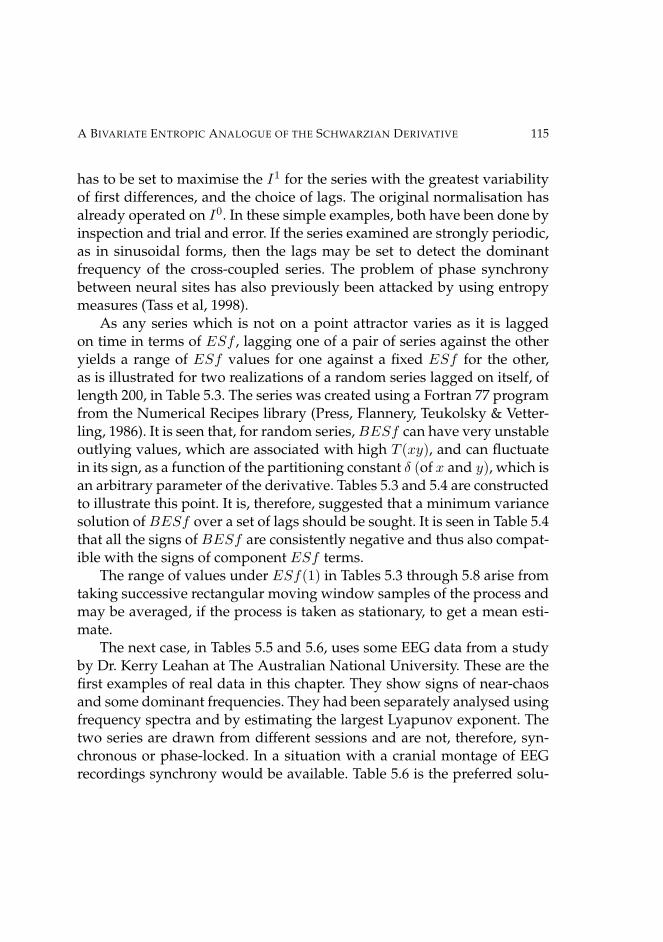
A BIVARIATE ENTROPIC ANALOGUE OF THE SCHWARZIAN DERIVATIVE 115
has to be set to maximise the I1 for the series with the greatest variabilityof first differences, and the choice of lags. The original normalisation hasalready operated on I0. In these simple examples, both have been done byinspection and trial and error. If the series examined are strongly periodic,as in sinusoidal forms, then the lags may be set to detect the dominantfrequency of the cross-coupled series. The problem of phase synchronybetween neural sites has also previously been attacked by using entropymeasures (Tass et al, 1998).
As any series which is not on a point attractor varies as it is laggedon time in terms of ESf , lagging one of a pair of series against the otheryields a range of ESf values for one against a fixed ESf for the other,as is illustrated for two realizations of a random series lagged on itself, oflength 200, in Table 5.3. The series was created using a Fortran 77 programfrom the Numerical Recipes library (Press, Flannery, Teukolsky & Vetter-ling, 1986). It is seen that, for random series,BESf can have very unstableoutlying values, which are associated with high T (xy), and can fluctuatein its sign, as a function of the partitioning constant δ (of x and y), which isan arbitrary parameter of the derivative. Tables 5.3 and 5.4 are constructedto illustrate this point. It is, therefore, suggested that a minimum variancesolution of BESf over a set of lags should be sought. It is seen in Table 5.4that all the signs of BESf are consistently negative and thus also compat-ible with the signs of component ESf terms.
The range of values under ESf(1) in Tables 5.3 through 5.8 arise fromtaking successive rectangular moving window samples of the process andmay be averaged, if the process is taken as stationary, to get a mean esti-mate.
The next case, in Tables 5.5 and 5.6, uses some EEG data from a studyby Dr. Kerry Leahan at The Australian National University. These are thefirst examples of real data in this chapter. They show signs of near-chaosand some dominant frequencies. They had been separately analysed usingfrequency spectra and by estimating the largest Lyapunov exponent. Thetwo series are drawn from different sessions and are not, therefore, syn-chronous or phase-locked. In a situation with a cranial montage of EEGrecordings synchrony would be available. Table 5.6 is the preferred solu-

116 INFORMATIVE PSYCHOMETRIC FILTERS
Table 5.3Values of ESf and BESf on a lagged random series
partitioning constant = .04lag ESf(1) ESf(2) BESf(1,2)0 -.60339 -.60339 .13711 -.61201 -.60339 -.10672 -.60982 -.60339 .00213 -.61193 -.60339 -.80434 -.60849 -.60339 .70135 -.61339 -.60339 -.39976 -.61565 -.60339 .21067 -.62309 -.60339 .05318 -.63860 -.60339 -.61769 -.63388 -.60339 -.073010 -.62859 -.60339 -30.0559
Table 5.4Values of ESf and BESf on a lagged random series
partitioning constant = .038lag ESf(1) ESf(2) BESf(1,2)0 -.63087 -.63087 -1.61441 -.63989 -.63087 -1.21942 -.63779 -.63087 -.78113 -.64043 -.63087 -5.55404 -.63441 -.63087 -3.94935 -.63874 -.63087 -1.99706 -.64264 -.63087 -1.49327 -.65229 -.63087 -.47458 -.67449 -.63087 -.00969 -.67168 -.63087 -.170010 -.66082 -.63087 -1.0143

A BIVARIATE ENTROPIC ANALOGUE OF THE SCHWARZIAN DERIVATIVE 117
tion.Another pair of EEG series is presented in Table 5.12, that has been
drawn from a real library www.physionet.org example, which is a syn-chronous pair but about which no physiological details concerning loca-tion and experimental conditions are known. As those details are missing,it is relegated to the Appendix merely for illustration of the instability thatBESf can have.
The ESf values are of comparable magnitude to those given in Table5.5, the D and H values were computed as in Table 5.2 for Γ series.
————————————————-Table 5.5
Values of ESf and BESf on two EEGseries under relaxation conditions
partitioning constant = .07lag ESf(1) ESf(2) BESf(1,2)0 -.66070 -.54500 .03881 -.65467 -.54500 .05122 -.65213 -.54500 -.75963 -.64850 -.54500 -.12074 -.65046 -.54500 -.75275 -.64447 -.54500 .26556 -.64480 -.54500 -.08167 -.66602 -.54500 -.63908 -.68870 -.54500 -1.38499 -.70055 -.54500 -.657910 -.73027 -.54500 .4720
————————————————-
The third example, in Tables 5.7 and 5.8, is created by using two strictlyperiodic series
x1,j = a1 · sin(b1 · j) + a2 · cos(b2 · j) [5.9]
x2,j = a2 · cos(b2 · j) [5.10]

118 INFORMATIVE PSYCHOMETRIC FILTERS
Table 5.6Values of ESf and BESf on two EEG
series under relaxation conditionspartitioning constant = .10
lag ESf(1) ESf(2) BESf(1,2)0 -.73528 -.48770 -.12261 -.72137 -.48770 -.31592 -.70651 -.48770 -.34543 -.70323 -.48770 -.13764 -.70651 -.48770 -.40965 -.69632 -.48770 -.05656 -.69594 -.48770 -.05007 -.71949 -.48770 -.07258 -.74613 -.48770 -.38449 -.76490 -.48770 -.154610 -.79342 -.48770 -.4595
where a1 = 1.0, a2 = .5, and b1 = .7855, b2 = .4. The periodicity createsmarked variation in BESf as a function of the lags used. In effect we arehere sampling from a series using a moving rectangular window of fixedlength. It will be noted that some of the ESf values are now positive, aswas derived in a case from Table 5.1. Table 5.7 is the preferred solution,but this is not the result of an exhaustive search, merely illustrative. It ap-pears that cross-linkage between sinusoidal series, which are the easiestform of strictly periodic series to create (unless we consider Walsh func-tions), generates wild outliers in BESf . With the possible exception ofsome experiments in psychoacoustics using sinusoidal forcing functions,this example is really not very plausible for real data. The distribution ofBESf obtainable by Monte Carlo methods would need lag series manytimes longer that the illustrative tables presented here.

A BIVARIATE ENTROPIC ANALOGUE OF THE SCHWARZIAN DERIVATIVE 119
Table 5.7Values of ESf and BESf on twosinusoidal series, [5.9] and [5.10]
partitioning constant = .079lag ESf(1) ESf(2) BESf(1,2)0 -.39387 .13742 -5.78121 -.36826 .13742 -.44662 -.34948 .13742 -4.03723 -.28921 .13742 -1.15114 -.25154 .13742 -1.13205 -.17656 .13742 -6.00866 -.14426 .13742 -.55307 -.06312 .13742 -1.98038 -.00925 .13742 -1.53309 .04213 .13742 -.330010 .08161 .13742 -4.8755
Table 5.8Values of ESf and BESf on twosinusoidal series, [5.9] and [5.10]
partitioning constant = .08lag ESf(1) ESf(2) BESf(1,2)0 -.28765 .13260 -.93291 -.26615 .13260 -303.52402 -.24998 .13260 -146.93753 -.19211 .13260 -1.02894 -.15645 .13260 -.83545 -.08514 .13260 -10.55066 -.05563 .13260 -7.48547 .02019 .13260 -.18388 .06890 .13260 -.00009 .11239 .13260 -.308610 .14464 .13260 -1.1079
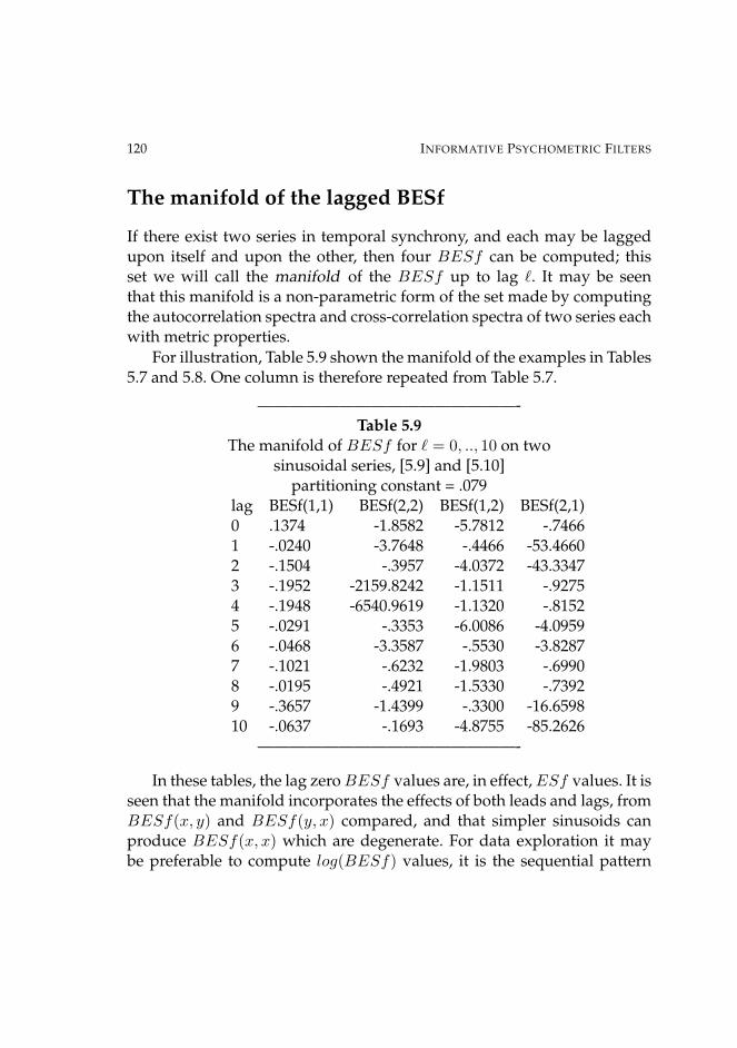
120 INFORMATIVE PSYCHOMETRIC FILTERS
The manifold of the lagged BESf
If there exist two series in temporal synchrony, and each may be laggedupon itself and upon the other, then four BESf can be computed; thisset we will call the manifold of the BESf up to lag `. It may be seenthat this manifold is a non-parametric form of the set made by computingthe autocorrelation spectra and cross-correlation spectra of two series eachwith metric properties.
For illustration, Table 5.9 shown the manifold of the examples in Tables5.7 and 5.8. One column is therefore repeated from Table 5.7.
————————————————-Table 5.9
The manifold of BESf for ` = 0, .., 10 on twosinusoidal series, [5.9] and [5.10]
partitioning constant = .079lag BESf(1,1) BESf(2,2) BESf(1,2) BESf(2,1)0 .1374 -1.8582 -5.7812 -.74661 -.0240 -3.7648 -.4466 -53.46602 -.1504 -.3957 -4.0372 -43.33473 -.1952 -2159.8242 -1.1511 -.92754 -.1948 -6540.9619 -1.1320 -.81525 -.0291 -.3353 -6.0086 -4.09596 -.0468 -3.3587 -.5530 -3.82877 -.1021 -.6232 -1.9803 -.69908 -.0195 -.4921 -1.5330 -.73929 -.3657 -1.4399 -.3300 -16.659810 -.0637 -.1693 -4.8755 -85.2626
————————————————-
In these tables, the lag zeroBESf values are, in effect,ESf values. It isseen that the manifold incorporates the effects of both leads and lags, fromBESf(x, y) and BESf(y, x) compared, and that simpler sinusoids canproduce BESf(x, x) which are degenerate. For data exploration it maybe preferable to compute log(BESf) values, it is the sequential pattern

A BIVARIATE ENTROPIC ANALOGUE OF THE SCHWARZIAN DERIVATIVE 121
over `, which is informative.The next real example is one which produced a surprise; it shows that
this method, though crude, can have some heuristic value, in that it leadsus to ask different questions about how the data are generated.
Recordings of spike trains per second in the visual cortex of an anaes-thetised cat were recorded by two independent tungsten-in-glass micro-electrodes with tips about 0.5mm apart. Each stimulus induces a brief timeseries in the two neurons being recorded; call each such train an epoch. Theonset times of the two parallel series in an epoch are synchronised; thereare no lag effects shown in Table 5.10. There are other parallel responseseries under a control condition which are not examined here.
Table 5.10 gives the values of ESf and BESf for the first 33 epochs.Though the original data analysis in terms of correlations (not done by me)suggested that the cells were not coupled, the pattern in Table 5.10 sug-gests that they are in terms of some weak dynamics. Such weak synchro-nization during conscious perception has been reported by Srinivasan,Russell, Edelman and Tonini (1999). This can be checked by using sur-rogate series methods (Theiler et al, 1992), but there are reported statisticaldifficulties with such methods. In dynamical terms, this suggests an hier-archical nesting of recursive maps. Dynamics in brain activity, arising asa consequence of stimulation as complicated as this have been reportedby Freeman (1999). He suggests that input from receptors increases thestrength of interactions between neurons, so that a loss of degrees of free-dom is entailed.
Discussion
There are many ways in which the parallel dynamics of two evolving pro-cesses can be coupled, even in the simplest cases which presuppose sta-tionarity both in the component processes themselves and in the cross-linkage. For example, the resultant series may be a weighted average, avector sum, a convolution, or, as here, a transmission of information.

122 INFORMATIVE PSYCHOMETRIC FILTERS
Table 5.10: Cat visual cortex V1 epochs
Epoch N ESf(1) ESf(2) BESf(1, 2)1 60 -.4632 -.5421 -1.21572 115 -.7450 -.6601 -2.41153 60 -.9041 -1.1539 -3.59104 60 -.6069 -.8327 -2.05535 40 -1.2018 -.9096 -1.48736 40 -.2575 -.2011 -.44597 40 -.6027 -.5572 -1.89368 30 -.6307 -.7876 -1.04109 35 -.3268 -.3320 -2.4721
10 35 -.3232 -.3959 -1.542311 35 -.4132 -.5221 -4.669712 60 -1.4888 -.9453 -1.329313 30 -.2093 -.2617 -.810914 50 -.9420 -.8911 -.255215 40 -.5771 -.6522 -7.073516 30 -.5497 -4820 -1.063817 45 -.9888 -.8400 -1.451218 40 -.2526 -.2060 +.110419 40 -.2816 -.3953 -2.663720 60 -.4522 -.5129 -.204221 60 -1.0393 -.9636 -1.887922 40 -.9117 -.6467 -1.539223 35 -.5436 -.5366 -1.395524 50 -.2620 -.2982 +.026625 30 -.4151 -.3652 -.729926 30 -.6285 -.6636 -8.929227 55 -.7805 -.6349 -.454528 50 -.3448 -.3656 -.650729 50 -.6630 -.8119 -1.200330 40 -.6088 -.6158 -1.180631 20 -.4625 -.5934 -2.867432 30 -.6346 -.6642 2.152933 40 -.2985 -.3468 +.9147
In this table N is the effective time series length within the epoch as anal-ysed.

A BIVARIATE ENTROPIC ANALOGUE OF THE SCHWARZIAN DERIVATIVE 123
The index BESf is, from our tentative exploration of its properties,not particularly easy to interpret. It would seem wise always to preservethe two ESf indices as well, as has been done in the Tables, and to com-pute the manifold if little is known a priori about the dynamics involved.If large reference samples are created against which any empirical reali-sation may be compared, then the type of the dynamics involved can po-tentially be identified. In this sense, ESf resembles (but is not reducibleto) the Hurst exponent of a time series (Feder, 1988). However, the originalmeaning of the Schwarzian as a measure of expansiveness is probably lost,a better intuitive interpretation is one of information impoverishment in arestricted sense.
There are two reasons why computation of ESf and BESf may beuseful: to identify the dynamic signature of the process, just as the Lya-punov exponents are used in chaotic dynamics, or to match against a givenreference sample in order to test for stationarity in the outputs of a process,even if the underlying dynamics of that process are not fully understood.It is critically important that the phase lock is known, if two series are syn-chronous, and that the increment (j in [5.9], [5.10] for example) is the same,or a known multiple in one series of the other, in real time units for two ormore series compared.
The comments raised here do resemble observations of Tass et al(1998), in particular, the need to try to circumvent the ”hardly solvabledilemma ’noise versus chaos’ irrespective of the origin of the observedsignals” (op cit. p.3293). It is now known that phase synchronisation ofchaotic attractors can arise or be induced (Chua, 1999) and a sort of phaselocking may be observed. The amplitudes of synchronised systems can re-main chaotic and affect the phase dynamics in a way that also arises as aconsequence of the presence of external noise. Local phase slips may beobserved, which means over a long series the question of synchronicityis irresolvable. Tass et al (1998) make the important point that synchroni-sation is not the same thing as cross-correlation, so instead of using thealgebra of linear time series statistics, they proposed two measures, one ofwhich, like ESf and BESf , is based on entropy.
The physiological data we have seen so far and been able to anal-

124 INFORMATIVE PSYCHOMETRIC FILTERS
yse, from the cat study and now from some data provided by thewww.physionet.org site, whose exact cortical source is not given, bothindicate that BESf might show long periodicities. Those long periodici-ties seem to emerge uncorrelated with the observed structure of the ESfsequences. There is some evidence that binding between closely adja-cent neural locations is mediated by 40Hz activity (Llinas & Ribary, 1993;Singer & Gray, 1995) in which case, sampling at 300Hz for ESf series wouldshow 40hz as a slower quasi-periodicity in BESf. This fundamentally im-portant matter needs more data for its resolution.
One advantage we would claim for our approach here is that relativelyshort series can be explored. This is important when the non-stationarityof psychological data is so often apparent and the need to compare shortepochs associated with specific known or suspected stimulus interventionarises. Schiff et al (1996) note the necessity of identifying the direction ofcausality in bivariate linkages and also confirm that systems with nonlin-ear cross-correlation will show mutual nonlinear prediction when stan-dard analyses with linear cross-correlation fail. This matter has also re-ceived comment from Vinje and Gallant (2000). To revert to the nonlinearpsychophysics which first motivated this study, the series we observe areinterpreted as trajectories and the coupling between them is dissipative.The theory of such coupling involves what is called ‘stochastic synchroni-sation’, which is a topological concept assuming a mapping up to a diffeo-morphism between nonlinear attractors, but its identification so far neces-sitates using delay coordinates (a standard method in the identification ofchaotic dynamics), which demands longer series than in the examples werealistically can obtain in psychophysics.
Note
The programs used here for ESf and BESf were written by the au-thor using Fort77 in a Linux environment. I am indebted to Kerry Lea-han for the use of some of her EEG data, to Dr Mike Calford for datafrom psychobiological research, to the Senior Vice President of the Temple-ton Group for providing me with an economic time series and to Michael

A BIVARIATE ENTROPIC ANALOGUE OF THE SCHWARZIAN DERIVATIVE 125
Smithson for pointing out the partial resemblance to the Hurst index. Thisweak resemblance is illustrated in the example from economic data in theappended table.
Appendix: Bernstein economic data and Physionetdata
Table 5.11 shows an analysis of a series of monthly values of an economicindex which was devised by a New York investment consultancy, Bern-stein, in the form of integer values that range from -7 to +10, reflectingthe under- or over-valuation of stock. It was used for illustration by theTempleton Global Growth Fund in its 1999 annual report, as a histogramgraph.
TheESf , fractal dimensionD, and Hurst indexH for each subseries of90 days are at the foot of the table, below the autocorrelation spectra. Theautocorrelation coefficients are carried through to 13 lags because the dataare monthly and some annual cycling might be in evidence around lag 12.It is not, however. These subseries are too short for ideal computation ofthe various indices, but the whole series is very non-stationary and non-linear.
The interest lies in the increasing instability of the dynamics as late1999 is approached. UsingESf it is seen that the increasing unpredictabil-ity is continuous from 1970 onwards, whereas usingH the anti-persistenceincreases only in the last epoch. Note that the series becomes relativelyunstable in the last column; this is what economists call ’volatility’, whichappears here to be a mix of high variance and antipersistence. In termsof giving advice to investors, it means that fund managers are, unsurpris-ingly, less confident in making predictions when volatility is high.
Each of ESf , D and H are filters. Each preserves and destroys infor-mation in an almost unique way. To get more insight into the evolvingdynamics it can be expedient to use all three, and even more indices. Oneindex suggests that there might be an abrupt change in the dynamics, ajump into volatility, another suggests that the rot had insidiously begun

126 INFORMATIVE PSYCHOMETRIC FILTERS
quite some time previously. As used here, all three filters smudge out thedynamics within data blocks, so that to search for a hypothetical sharplocus of a dynamical change at one month other filters would be needed.

A BIVARIATE ENTROPIC ANALOGUE OF THE SCHWARZIAN DERIVATIVE 127
Table 5.11 The Bernstein-Templeton Economic SeriesThe four successive periods are 90, 90, 90 and 89 months long respectively.
Period; Feb 1970→ Aug 1977→ Feb 1985→ Aug 1992→——- ——- ——- ——- ——-mean -.389 -.044 -.633 .000
s.d. 1.590 1.763 1.792 2.152min -4 -7 -7 -5max +4 +4 +3 +10
——- ——- ——- ——- ——-ar1 -.0481 .0057 .0763 .5024ar2 .0180 -.1262 -.1570 .1481ar3 -.0223 -.0008 .0596 .0194ar4 -.1248 -.1293 .0013 .0850ar5 .0170 .0424 .0584 .1384ar6 .0627 .0421 .0280 .0388ar7 -.1342 -.0116 -.0326 -.1238ar8 .0357 -.2510 -.0015 -.1893ar9 -.0141 -.1511 -.0800 .0461ar10 -.0675 -.0745 .0697 .0704ar11 -.1175 .1140 .2486 .0874ar12 -.0735 -.0080 .0760 .0558ar13 -.1401 -.0834 .0063 .0049
——- ——- ——- ——- ——-I1 2.1474 2.0751 1.7980 2.1197I2 1.9214 1.9260 1.8279 1.9474I3 1.9421 1.9840 1.7050 1.3642
——- ——- ——- ——- ——-ESf -.2965 -.3361 -.6019 -.6225D 1.3996 1.4354 1.4235 1.1015H .6004 .5646 .5765 .8985

128 INFORMATIVE PSYCHOMETRIC FILTERS
Table 5.12: D,ESf,BESf in a Physionet EEG series3 msecs time intervals, recordings in µvolts
segment D(2) ESf(1) ESf(2) BESf(1,2) BESf(1,2,1)1-100 1.9121 -.4607 -.4225 -1.3548 +.4376
101-200 1.7592 -.4577 -.3633 -1.1785 -.5894210-300 1.7469 -.2760 -.3588 -.2902 +.1218301-400 - -.4715 -.5906 -.4803 -2.2851401-500 - -.6452 -.5974 -2.9476 -1.5224501-600 - -.7287 -.5790 -.3100 -.1625601-700 - -.4462 -.5339 -.4956 -.6827701-800 - -.4621 -.4997 -2.3512 -.1527801-900 - -.6054 -.4259 +.9309 -4.1840
901-1000 - -.4133 -.3916 -.0529 -.04901001-1100 1.7882 -.3611 -.3402 -2.3839 -.34681101-1200 1.8602 -.5401 -.5729 -.4712 -1.92691201-1300 1.7737 -.5171 -.4922 -1.2113 -.23121301-1400 - -.3791 -.4328 -.1580 -.19621401-1500 - -.2443 -.2619 +.0242 -.11541501-1600 - -.8589 -.4347 -.5036 -1.74371601-1700 - -.4356 -.4266 -.1498 +.01141701-1800 - -.3860 -.5122 +.0733 -.5679
——- ——- ——- ——- ——-
D(2) is the estimated fractal dimensionality of the second series. It has onlybeen computed where it showed possible instability.BESf(1,2,1) means the cross-Schwarzian with the second series lagged byone step.

Chapter 6
Tribonacci and Long Memory
There are various ways of constructing systems that jump in their dynam-ics from one configuration to another. Systems that move from edge-of-chaos into a sort of saturated stability as their complexity increases areconsidered to be a basis for a new sort of thermodynamics where entropyis not always increasing, but the complexity of both a biological systemand its connected potential environment are increasing together (Kauff-man, 2000). This chapter uses a completely artificial model whose proper-ties can at least heuristically provide illustrations of qualitative jumps indynamics, some of which are irreversible, unlike transitions through cuspcatastrophes, and identify some of the results of relaxing purely determin-istic dynamics into partly stochastic constructions. Identifiability is againa central theme of our explorations. As this is a complicated topic a shortpreamble of the chapter follows.
Time series processes which can be derived from the Tribonacci seriesby damping its explosive properties are examined. A modification of theTribonacci series formed by imposing a modular constraint on its expan-sion, called Tribmodk, is used to illustrate the effects of small changes in itsparameters on a diversity of statistical properties variously used to char-acterise a quasi-periodic trajectory, which may be suspected to be chaoticor at the edge-of-chaos and almost certainly falls into the family of tran-
130 INFORMATIVE PSYCHOMETRIC FILTERS
sient nonlinear nonstationary series that arise in psychology. The entropicanalogue of the Schwarzian derivative, ESf, is again used, in first-orderand higher-order analyses, and the potential use of the Tribmodk series asa source of time series in psychophysical serial extrapolation experimentsis noted. These series create conceptual problems in distinguishing in hu-man sequential performance between identification, estimation and pre-diction. Comparative analyses, falsely assuming that the process is purelystochastic and stationary, are tabled to show that the process can be de-scribed but not functionally mapped by excessively complicated classicalARMA modelling. Mixing deterministic and stochastic components hascomplicated consequences, not necessarily diminishing the stability of thetrajectories.
There are two main ways in which one might want to try and explorethe relation between an observed data string made up of human responsesand the nonlinear process that leads to its observable evolution throughsome sequences of filtering: one is to create a process that is known fullyin its algebra to be nonlinear, use it as a stimulus generator, and see whatresponses it evokes in sequence over time; the other is to start with prop-erties of the observable response sequence and conjecture what nonlineardynamics might have produced it. The first is found in the few experimen-tal studies that have used series extrapolation as a dynamic response task,and the second is to start with simple series, such as point processes, anduse a known nonlinear attractor to produce the inter-stimulus responseinterval statistics. Both can be found in the relevant literature; the second(Han, Kim & Kook, 2002) is mathematically better understood but is psy-chophysically useless because it relies too readily on the generation of longseries under stationarity.
In psychophysiological data there are various sorts of sequences: re-sponse that vary in magnitude with the same time intervals between them;series of time intervals with the same point processes (of unit magnitude)that are recorded; and series that involve both at the same time variable in-tervals between events and variable magnitude events. The third sort are,in principle, the most interesting.
A fundamental difficulty lies in determining what is a close copy or
TRIBONACCI AND LONG MEMORY 131
an extension of the trajectory of a dynamical process. Given some series,it is not impossible for the human observer, by a sort of dynamical ex-trapolation, to create a few further terms which match it in the first twomoments; but it is not expected that the full autocorrelation spectra of theprocess could be matched for something like an ARMA process. If the gen-erator of the series is nearly chaotic, then the observable output may haveembedded in it local short epochs that are quite predictable, separated byepochs that are indistinguishable from random evolution (Geake & Greg-son, 1999). The random parts are predictable in their first two momentsand effectively stationary therein; the recurrent short arpeggio-like pat-terns are identical copies of one another but their onsets are not predictableby simple extrapolation. The use of the Lyapunov spectra to characterisea chaotic sequence rests on the property that prediction is locally possiblebut falls off exponentially with extrapolation into the future. Predictabil-ity of mixed chaotic and stochastic processes may be viable if the resolu-tion of prediction of individual terms is only with a predetermined limit±ε. What is predictable mathematically in a simulation exercise is not thesame as prediction performance by human observers, but the first may beused as a baseline measure of prediction efficiency.
If it is seriously contended that the process by which a human observercreates series of responses without feedback is analogous to the tracingout of an attractor trajectory on the invariant manifold, then the Poincaresections (plotted as re-entry maps) of the theory and data strings may begenerated and compared under stationarity. It does not necessarily followthat the prior creation of a stimulus series can overwrite the internal dy-namics of response generation once the stimulus series is discontinued.There may be two different attractors involved.
Psychological models of perception and memory usually make provi-sion for three boundary conditions, a short-term memory of limited capac-ity feeding into long-term memory of almost unbounded capacity, and anupper bound on the range of admissible sensory inputs. There are othermemory systems now experimentally identified (Baddeley & Logie, 1999),but this distinction between transient working memory and the storage ofretrievable memories of various sorts is generally accepted. For a human

132 INFORMATIVE PSYCHOMETRIC FILTERS
observer to observe Un−1, Un−2 and Un−3 and then respond with Un re-quires holding previous terms in memory. Three terms is probably withinthe capacity of short-term working memory. Modelling of this may bedone in a diversity of mathematical ways, here one of the simplest formsof such a process model is used to illustrate how time series with nonlin-ear properties result from the imposition of the boundary conditions. Thesubsequent analysis of the identifiable statistical properties of the series isexplored with a diversity of measures.
The Tribonacci Series
A recurrence relation, which is sometimes called the generator of the Tri-bonacci series, by a humorous analogy with the much better known Fi-bonacci series, is
Un = Un−1 + Un−2 + Un−3 [6.1]
where Un usually is taken to have only real positive integer values, andhas as its equation for deriving its roots as
x3 − x2 − x− 1 = 0 [6.2]
Unlike the Fibonacci series [6.2] has only one real root, which is
η = 1.83928675521416...
and is not transcendental.Cundy (2000) notes that η can be given an explicit value, which is
η =13[1 + (19 + 3
√33)1/3 + (19− 3
√33)1/3] [6.3]
and he lists some curious and useful properties of η, such as
(η − 1)(η2 − 1) = (η + 2)(η − 1)2 = 2 [6.4]
orη4 + 1 = 2η3, and thus η + 1/η3 = 2 [6.5]

TRIBONACCI AND LONG MEMORY 133
Here an attempt is made to examine some series derived from [6.1] whichdo not explode and hence might be of interest as models of stable timeseries with long internal memories but a limited capacity to expend energyor to store outputs. As Cundy (2000) notes, [6.1] is a truncated case of thegeneral equation
xn = xn−1 + xn−2 + ....+ x+ 1 = (xn − 1)/(x− 1) [6.6]
which has a solution x = 2 − 1/xn, that obviously approaches 2 steadilywith increasing n. We may also comment that as a process [6] is not sta-tionary in its order for the first (n− 1) terms.
It is apparent that n in [6.6] is an assumption about the short-termmemory of the system, and is taken to be a constant independent of U .Let us call this the order of the memory and denote it by m, to leave nfor use as a general suffix. In real experimental memory data, the capacityof the component memories is not observed to be constant, and m couldtherefore be better treated like a variable. This does not affect the analysesin Tables 6.1 and 6.2.
Let us rewrite [6.1] in two different ways and explore each separately.First, dampen the cumulative nature of [6.1] by rescaling1 any term Un >10 by mod10. So, if U1 = U2 = U3 = 1, to start the recurrence, then U4 = 3,U5 = 5, U6 = 9, U7 = 17.0(mod10) = 1.70, U8 = 15.7(mod10) = 1.57,U9 = 12.27(mod10) = 1.227, U10 = 4.497 and so on. Rewriting [6.1] wenow have
Un =Un−1 + Un−2 + Un−3 if Un ≤ kk−1Un if Un > k
[6.7]
where the role of k is to put an upper bound on responses to inputs, sothat the process does not explode. The need for such a bound has beenrecognised since Herbart in 1812 (cited by Gregson, 1988).
1 This is not modk in the proper sense, if it were, then, for example, Un = 17(mod10) wouldbecome Un = 7. If that definition of mod is used, then the series takes only integer valuesand could be represented as a Markov chain over k states.

134 INFORMATIVE PSYCHOMETRIC FILTERS
The important point to grasp is that this series is quasi-periodic2. Run-ning the first 200 iterations to three decimal places suggests that it is ap-proximately period 19; as 19 is a prime number, this is a curious prop-erty, not one associated with the more familiar bifurcation series or periodthree recurrences in chaotic dynamics. It then raises the question, does itlook like a series at the edge of chaos? In general, the series [6.1] can berewritten mod(k), so to give it a name let us call it Tribmodk. The relationbetween the modulus and the quasi-periodicity is unknown to me, but thequasi-periodicity is not observed to be constant over long realisations ofthe series. Then, the Tribonacci series is simply a case of m = 3. The rela-tions [6.2], [6.3], [6.4] will hold for subseries, that is segments between theoperation of mod(k), but not across that operation of [6.7].
The other modification of [6.1] is to write, more simply,
Un = q−1[Un−1 + Un−2 + Un−3], 0 ≤ q ≤ 1 [6.8]
which if q ' 3 becomes an AR(3) series, and if q ≥ 3 it runs onto a point at-tractor. This one we will call Tribarq. It is less interesting, so it is eschewedhere.
From runs 200 iterations long, with U1 = U2 = U3 = 1.0 it is possibleto estimate some statistical parameters of the Tribmodk process as a func-tion of the modulus k. The estimates of the fractal dimensionality D andthe Hurst exponent H are from an algorithm of West, Hamilton and West(2000) and their confidence limits are not known. MaxP is an estimate ofthe dominant periodicity from inspection of the autocorrelation spectrum;this is not necessarily constant over extrapolation. The largest Lyapunovexponent Λ1 is from SANTIS. The entropic Schwarzian analogueESf is aspreviously defined (Gregson, 2000), with partitioning constant .015. Sloperefers to mean∆1U .
The D and H values are not independent parameters, because they arelinked by the relation D+H = 2, and are included for illustration, but the
2 The use of modular algebra in maps with recurrent trajectories is not, of course, new. Itwas used in Arnold’s cat map in various forms to induce mapping on a torus (see Schuster,1984, p. 152 et seq.)

TRIBONACCI AND LONG MEMORY 135
Table 6.1Estimates of some statistical properties of Tribmodk
Property mod 7 mod 10 mod 13 mod 19Mean 2.6061 3.3798 4.3795 6.2192
s.d. 1.9040 2.8795 3.9187 6.0812slope -.0002 +.0012 +.0037 +.0031MaxP 40 19 9 41
D 1.8287 1.6925 1.6963 1.6562H .1713 .3075 .3037 .3438Λ1 +.1489 +.1305 +.0563 +.0519
ESf -1.9495 -2.4398 -.6758 +.4396————————————————-
remaining parameters each describe different properties of the series. Theapproach advocated here is to compute a diversity of measures to charac-terise adequately the peculiarities of the dynamics, including any evidenceof nonstationarity. This necessitates the further exploration in Table 6.2.
Some of the estimates of properties in Table 6.1 are reminiscent ofchaotic dynamics, so sensitivity to initial conditions is an aspect of Trib-modk that is worth examination. Perhaps the simplest way to investigatethe effects of varying initial conditions is to make a second-order changein one of the original starting values, replacing U1 by 1.01. In Table 6.2,this modified mod10 series is coded as S1. Alternatively, we may take anythree successive Un values from its evolving trajectory as a new startingpoint; as the series is deterministic, this will replicate the gradual changesin the local quasi-periodicity of the trajectory if these new subseries areconcatenated.
For example, the series S2 is created from the mod 10 column in Table1 by putting
U1(S2) = U170 = 3.991 [6.9.1]U2(S2) = U171 = 6.539 [6.9.2]U3(S2) = U172 = 1.163 [6.9.3]

136 INFORMATIVE PSYCHOMETRIC FILTERS
Figure 6.1: Graphs of four Tribmodk series for contrastTribmodk with k= 7, 10, 13 and 19

TRIBONACCI AND LONG MEMORY 137
The values for S3 and S4 are similarly lagged, U1(S3) = U340, U1(S4) =U510, each series is 200 iterations long, so that they overlap.
Table 6.2Variations in properties of Tribmod10 with starting values
Property S1 S2 S3 S4
Mean 3.3874 3.3931 3.3946 3.3435s.d. 2.8859 2.9068 2.8953 2.8139
slope +.0012 +.0015 -.0005 +.0005MaxP 19 9 9 19
D 1.6925 1.7012 1.8287 1.6882H .3075 .2988 .1713 .3118Λ1 +.1276 +.1120 +.1433 -.0010
ESf -2.4398 -2.4128 -2.4128 -2.4181
Higher-Order Derived Series
Given any series xj , j = 1, ..., n, it is possible to create other series byinternal multiplication across lags. The simplest series is then
Xk := xjx(j−k), j = 1, ..., n, k fixed [6.10]
and the family of Xk with k a variable defines the bases of the autocorre-lation spectrum of x.
If the multiplication is taken to a higher order, then
X(m,n) := xjx(j−m)x(j−n), ∀m,n m ≤ n [6.11]
andX(m,n) is sometimes, in frequency domain analyses, called a bispectralseries. IfX(m,n) is computed over a set ofm,n values, it gives us a triangu-lar matrix of series, which, because the process [6.11] is symmetric in m,n,can be treated as the off-diagonal cells of a square skew symmetric matrix,M of size n× n.

138 INFORMATIVE PSYCHOMETRIC FILTERS
Each cell in the X(m,n) matrix may be replaced by a function of theseries. In this context, we may compute the ESf of each of the X(m,n), andfor convenience write
b(m,n) := ESf(X(m,n)) [6.12]
The triangular matrix computed here for each of the Tribmodk series is ofthe form
b(1,2) b(1,3) b(1,4) b(1,5) b(1,6)b(2,3) b(2,4) b(2,5) b(2,6)b(3,4) b(3,5) b(3,6)b(4,5) b(4,6)b(5,6)
If this matrix is reflected to give the full square form, then its eigenvaluesare all real (Gregson, 2001), because all the elements b(m,n) are real andnot complex. It should be noted that the values of m,n are minimal andthus the matrix acts like a high-pass filter. If n were to be set at 2, 7, 10 ,13,19 respectively, then different values related to slower forced frequencieswould be found.
Table 6.3Eigenvalues for the Higher-order ESf
Eigenvalue k = 7 k = 10 k = 13 k = 19(1) -1.7448 -1.9506 -1.4773 -1.6390(2) -.7661 -.4573 +.4536 +.6265(3) +.5663 +.4114 -.3589 -.4952(4) +.3580 +.2667 -.2449 -.1892(5) -.2283 -.1775 +.2440 +.1627(6) +.1290 +.0286 +.0016 -.0557
Tables 6.3 and 6.4 were computed using only the first 200 iterations ofTribmodk. It is seen in Table 6.3 that the second through fifth eigenval-

TRIBONACCI AND LONG MEMORY 139
ues change sign as k increases. There is a reflection in the pattern of signsbetween k = 10 and k = 13.
Table 6.4Higher-order ESf matrices for the Tribmodk series
Values in italics lie within the 95% confidence intervals for random surro-gates
For k = 7-.2534 -.2598 -.2823 -.0627 -.0244-.3170 -.6473 -.4080 +.3047-.4117 -.4135 -.5552-.2605 -.0313-.2428 n: 4
For k = 10+.0281 -.3663 -.3118 -.1989 -.2875-.4510 -.5262 -.5393 -.1329-.3087 -.4255 -.1308-.5067 -.1954-.3430 n: 4
For k = 13-.3703 -.1928 -.3817 -.1260 -.0824-.1799 -.3469 -.3520 -.0276
+.0662 -.1696 -.1210-.5422 -.3138-.3143 n: 4
For k = 19-.3645 -.1545 +.0107 -.2939 -.4697-.3226 -.3355 -.0869 -.3339-.0167 -.1036 -.5846-.4247 -.3677-.1273 n: 2

140 INFORMATIVE PSYCHOMETRIC FILTERS
To show the pattern of the higher-order ESf values that generate theeigenvalues for the system, the triangular b(m,n) matrices are set out inTable 6.4. The n: values in Table 6.4 are the number of italicised valuesout of 15 in that triangular matrix. There is some agreement between theESf values in Table 6.1 and these n: values in that the k = 19 data aremore different from the other three series; as k increases resemblance to asimple strictly periodic or random series diminishes. The emergence of amore complex wave form is also shown in the graphs.
Discussion
If a series is generated by a nonlinear process, then the set of statistics tocharacterize it adequately has to be more than the sufficient statistics of alinear process with Gaussian residuals. This is so even under stationarityof the parameters generating the observed realization of the trajectory. Thesimplest statistics, then, can only serve as an exploratory way of findingsigns of suspected non-stationarity by examining successive sub-series. Ifthere is no reason to expect a simple analytic representation of the under-lying processes generating the trajectories then confidence limits on any ofthe statistical indices, such as used here, can only be estimated by MonteCarlo methods.
If series are short, as is deliberately the case here, and have many singu-larities, then attempting a representation through Fourier analysis is verycumbersome and, even with wavelets, would be potentially misleading3
Wavelets can handle Dirac δ functions when they arise within a reasonablylong process, but the singularities induced here with the mod jumps are ofa different form.
In Tables 6.1 and 6.2, the information provided by the slope merelyindicates that the process has no detectable shift in its mean over thesampled series length. In that limited sense, it is stationary and might bewithin the trajectory of a closed attractor. The ESf uses none of the in-
3 Kaiser writes, p. 61, of ”the tremendous inefficiency of ordinary Fourier analysis in deal-ing with local behaviour” (Kaiser, 1994).

TRIBONACCI AND LONG MEMORY 141
formation in the mean and s.d. and is sensitive to differences which arenot sufficiently captured in the s.d. H has low values, which is usuallyinterpreted to mean that the process is antipersistent (Feder, 1988).
The difference in terminal values for S1 in Table 6.2 andmod10 in Table6.1 is simply due to setting U1 = 1.01 as against U1 = 1.0. These values arerespectively
U198(S1) = 9.915, c.f. 9.893 [6.10.1]U199(S1) = 1.879, c.f. 1.875 [6.10.2]U200(S1) = 1.964, c.f. 1.960 [6.10.3]
which indicates that trajectories initially separated do not converge ontothe same values over the range explored. Nor, however, do they widelydiverge, which is compatible with the small positive Λ1 values.
The variations in Λ1 and in ESf over successive epochs are smalland may be due to computational approximations in the relevant algo-rithms, but there is evidence from recurrence plots that some period ofnon-stationarity does emerge within the longer series U1, ..., U510, andthe pattern of peaks in the autocorrelation spectra changes and becomesmore complicated with evolution. For the mod19 series, the autocorrela-tion spectra and the recurrence plot become even more complicated andqualitatively different from the lower modk series. This is reflected moreobviously in the ESf value, which becomes positive (this shift in sign hasbeen found previously in varying parameters in edge-of-chaos series), ascompared with the changes in the other statistics.
It is obvious from Table 6.1 thatESf is very sensitive to the choice of k,but equally within one k value it may be insensitive to local second-orderchanges in the evolution of the same trajectory, as seen from the twin val-ues of−2.4128 in Table 6.2. This insensitivity can arise as a consequence ofthe choice of the partitioning constant δ (See Appendix). The higher-orderESf matrices can be used to compare the dynamics in successive shortconcatenated subseries, particularly to explore for evidence of nonstation-arity, as they can reveal subtle changes that are missed by the lower-orderparameters; this has been done for some EEG series (Gregson, 2001).

142 INFORMATIVE PSYCHOMETRIC FILTERS
The conventional way of comparing the series, as they are obviouslyquasi-periodic, is to compute their Fourier Power Spectra, provided thatwe bear in mind the warnings just given. For illustration, spectra for Trib-modk k = 7 and 19, iterations 1-200, are shown; the extra secondary peaksthat emerge as k increases are apparent, as is a shift in the location andpower of a major peak in the middle range.
Figure 6.2: Graphs of Fourier Power Spectrafor Tribmodk k = 7 and 19
The computation of D,H and Λ1 over very short series is associatedwith difficulties, even if only relative values are sought. There is, however,some evidence that in such circumstances, with series appreciably shorterthan the 200 used here for illustration, that ESf can still be informative,and can differentiate between stochastic and some nonlinear deterministictrajectories (Gregson, 2000b). It is trivially simple, using ESf , to differen-tiate between strictly periodic series and quasi-periodic ones, because forstrictly periodic series the successive differences eventually vanish. Theydo not vanish for Tribmodk, which can have a somewhat curious distri-

TRIBONACCI AND LONG MEMORY 143
bution of ∆4(Un). Tribmodk is an example of a process which is strictlystationary in its parameters but, if examined by calculating the range ofdescriptive statistics now available for characterising non-linear dynam-ics, will appear in the light of some to be non-stationary in its outcomes.Such processes are not novel, the SETAR series created by Tong (1983) arecases in point.
The reader might appreciate some hint as to how one might use theTribmodk family and its associated statisticsm, k in experimental psychol-ogy. Perhaps the simplest way is to use a series extrapolation task, wherethe theory is used to generate a stimulus display over time and then thesubject is asked to continue the series for another large number of trials4.This has been done by various authors with the logistic or Henon func-tions (Neuringer & Voss, 1993; Smithson, 1997; Ward & West, 1998; Heath,2002), and comparisons made between the recurrence plots of theoreticaland response time series. Recurrence plots are not helpful for short series,because of their sparsity, but other statistics such as ESf can be used forcomparisons of theoretical and response series, even when the series arereplete with singularities.
There are deep relations between the chaotic dynamics of complex cu-bic maps on the unit interval, their attractors and the Fibonacci series, andthe Schwarzian derivative, that have been explored by Milnor and his co-workers (Lyubich, 1993). This suggests that, in terms of topology, thereare a number of unanswered questions about the series used here. It isan open question whether Tribmodk should be called chaotic, in the strictsense used to describe a strange attractor, despite the positive value of itsestimated largest Lyapunov exponent. It is a closed trajectory on an in-variant manifold and, with increases in the one parameter k, it becomesmore complicated, but not in the period-doubling sequence of, say, theRuelle-Takens series. It is, perhaps, preferable to call it simply nonlineardeterministic and stable. Other such series with local memory have beenalso described (Morariu, Coza, Chis, Isvoran & Morariu, 2001) in com-
4 This type of experiment has also found use in clinical diagnosis (Helmuth, Mayr & Daum,2000) with some simplification.

144 INFORMATIVE PSYCHOMETRIC FILTERS
paring and contrasting human with theoretical memory processes. Thereare yet other ways of creating chaotic sequences by considering quadraticmaps with no real zeroes. The main result is that rational initial conditionsproduce finite or infinite periodic sequences, whereas irrational ones yieldinfinite but not periodic sequences (Carvalho, 2002, p. 31).
Classical ARMA analyses
It can be informative to see what linear ARMA(p.q) representations of theTribonacci series look like. The solutions are limited to models with p 6>5, q 6> 5. We note that the order of fitted q increases with k, but the valuesof the p terms change irregularly.
————————————————-Table 6.5: ARMA parameters for the four Tribonacci series
parameter Trib07 Trib10 Trib13 Trib19AR1 -.2203 .3214 .1125 .1049AR2 .2169 -.3448 -.2658 .0674AR3 .1025 .6165 .1415 -.1006AR4 .2961 -.1432 .4127 .0387AR5 .6046 .5498 .5986 .8857
MA1 -.0067 -.5429 .2484 -.1373MA2 -.6222 -.1241 .0752 -.1031MA3 -.2929 -.5964 -.1545 .1808MA4 .3003 -.2238 .2368MA5 -.8825 -.9437
-2logΛ .7181 .9168 .9675 1.1976
All the -2logΛ terms in both Tables 6.5 and 6.6 are to be read as × E+03.————————————————-
The point of this analysis is to show that, if we have a purely deter-ministic process, which is, if we know its generating function, perfectly

TRIBONACCI AND LONG MEMORY 145
predictable, and we instead assume falsely that it is purely stochastic andstationary, then an ARMA model is computationally derivable. But thismodel tells us nothing about exactly how the process evolves; it is descrip-tive and not functional. It discriminates between the forms of Tribmodk ifk is increased, but does so in a way that is much too complicated comparedwith the generating function. It thus violates Occam’s Razor.
Paradoxically, this ARMA analysis could have some use, though itfurnishes no real insights. If Tribmodk is used as the seed process in aserial extrapolation experiment and the subject is in fact capable of ex-trapolating within some tolerance bound, ε, then the ARMA model ofthe subject’s extrapolation should resemble an appropriate minimum or-der ARMA(p,d,q), and that should also be a good fit to the ARMA(p,k,q)model of the generating seed series. We note that it is highly implausiblethat the strategy used by a human observer would be isomorphic with anARMA model with 8 to 10 terms in a linear expression, as shown in Table5. The brain does not store information that way.
Differencing at lag k, as shown in Table 6.6, does not make muchchange to the overall goodness of fit index -2logΛ, but the structure of theARMA models does change, and the differences between Tribmod13 andTribmod19 are apparent, particularly the collapse of the order of the MAterms. It is worth re-emphasising that these induced complicated patternsare all the consequence of changing just one real positive scalar parameterin Tribmodk.
ApEn modelling
Pincus, in a series of analyses (see, for example, Pincus, 1991, Pincus andSinger, 1998), has shown that a measure of approximate entropy (ApEn),which can be applied to relatively shorter time series, will qualitativelydistinguish between some stationary processes, where other measuressuch as LLE or D2 are not reliably computable. It can be shown from avariety of cases that ApEn is not monotonic on ESf, and that ESf can dis-tinguish between some pairs of series, including the Tribmodk series used

146 INFORMATIVE PSYCHOMETRIC FILTERS
Table 6.6: ARMA parameters with differencing at level k
Parameter Trib07 Trib10 Trib13 Trib19AR1 .1283 .4038 .5632 -.5944AR2 -.0799 -.2599 -.4054 -1.4286AR3 -.6251 -.0374 .3901 -.9088AR4 .5806 -.7429 -.8611 -.7501AR5 .6015 -.6007
MA1 -.2608 -.6675 -1.0313 .3037MA2 -.7149 -.1765 -.2128 .9979MA3 .6554 .0764 -.0215MA4 -.2574 .6673 1.2268MA5 -.4073 -.8079 -.7046
-2logΛ .7395 .9384 .8470 1.1267
————————————————-
here, rather better than ApEn. The two measures do not use the same dataproperties.
The estimated ApEn values, using m = 2, r = .20 (the parameters ofchoice in ApEn), for the Tribmodk series are, in order of increasing k,
.5133, .5625, .5143, .5117
These values should be compared with the ESf values in the last row ofTable 6.1.
Modified Tribonacci series with one control parameter k are strictlydeterministic. If k is replaced only when it serves as a divisor by a randomvariable θ, where 1 ≤ θ ≤ k, then the process becomes different in itsevolution, but is still bounded and edge-of-chaos. Numerical comparisonsof solutions to the ESf and ARMA modelling of the series are provided;the effects of introducing stochastic noise appear to be irregular and to bediminished as k is increased.

TRIBONACCI AND LONG MEMORY 147
There have been a number of studies concerned with the identificationand analysis of processes that are reasonably believed to be a mixture ofnonlinear dynamics and random noise. Such processes may be treated asa mix of low dimensionality dynamics and high dimensionality stochasticbackground, or as nonlinear dynamics masked by stochastic noise of in-determinate structure. The degree of masking is critical for identificationof the deterministic components. In short data samples, it may be impos-sible to disentangle signal from noise if we regard the nonlinear dynamicsas generating the true signal. Misidentification of dynamics thus arises ifone uses methods that presuppose the presence of, and only of, stochasticdynamics. At the same time, biological processes are considered to be con-taminated ubiquitously with noise, or even require for their viable plastic-ity the presence of random components (Schaffer, Ellner & Kot, 1986).
The Tribmodk series could be interpreted as a model of some cognitiveprocess. In fact, if it is used as a stimulus generator for serial extrapolationtasks, then, if the subject does extrapolate most of the properties of theseries whose local evolution has been presented, it can be thought of asevidence that the brain can perform the operations intrinsic to Tribmodk.
Tribmodk is built on three deterministic operations: (i) storage of a fewnumerical values in short-term memory, (ii) addition, and (iii) rescaling bysomething like shifting a decimal point or division by an integer. These areall simple operations that are used in AI neural networks and thought tobe performed in real neurophysiological connected structures (Oprisan &Canavier, 2001). It is important to note, from inspection of the graphs inthe previous study, that Tribmodk depends on its starting values for a fewterms and then runs onto an attractor.
The parameter k in fact performs two distinct roles: a time marker,which has been called a modulus but which triggers the action of the divi-sor, and the divisor itself. Let us relabel these kt and kd respectively, in ef-fect increasing the number of free parameters in the model by one. Now letus replace kd by θd, where 1 ≤ θd ≤ k and θd ∼ rect((k+1)/2, .289(k− 1)),where rect is a random i.i.d. distribution on the interval. In doing this, amixed deterministic-stochastic process has been created. As each of kt andkd could be replaced by a bounded random variable, there are four possi-

148 INFORMATIVE PSYCHOMETRIC FILTERS
ble Tribmod models; deterministic ktkd, mixed ktθd, θtkd, and stochasticθtθd. The purpose of this part is to compare the properties of Tribmodkand Trbmodktθd.
A secondary modification is to admit the range of θ not over 1 ≤ θ ≤ kbut only over k ± 1, which is illustrated in some of the figures. Obviously,this is less disruptive of the dynamics.
ESf Analyses
The ESf analyses are computed in the same was as for the deterministicseries; there is a complication in that any realization of the series now isnot an exact replication of any other with the same seeds x1, x2, x3 and k,so there is variance in the evolution of the source trajectory as well as inthe surrogate randomizations.
In Table 6.7 it appears that, for k = 13, the process is more consistentwith being random. In all the other three series it is nearer to chaotic thanrandom, (as ESf is more positive, as shown in Gregson 2002) but the dif-ference (-.539 versus -.549) for k = 19 is very slight.
————————————————-Table 6.7: ESf and surrogate c.i. for the four Tribmodkθ series
surrogate: 95% c.i. 95% c.i.bounds: lower upper
k ESf7 -.2832 -.450 -.418
10 -.4801 -.616 -.58813 -.6736 -.675 -.61919 -.5390 –.583 -.549
δ = .03 in all cases.

TRIBONACCI AND LONG MEMORY 149
The interplay of k and θ on the emergent dynamics is obviously notsimple.
The higher-order ESf analyses may also be compared with the previousresults and are tabulated in the same fashion.
The magnitudes and signs of the Eigenvalues are changed and rela-tively diminished. There is a suggestion that the patterns converge as kincreases and the effect of the presence of a random component is less-ened.
————————————————-Table 6.8: Eigenvalues for ESf[b(m,n)]
Eigenvalue k=7 k=10 k=13 k=19(1) -.6165 -1.4637 -1.1527 -1.1440(2) -.4709 +.2256 +.4969 +.3358(3) +.2772 -.2219 -.3054 -.2443(4) +.1827 +.1590 -.2035 +.1009(5) +.0952 -.1124 +.0706 -.0954(6) +.0078 -.0368 -.0243 -.0420
————————————————-
It can be seen by comparing n: values in Table 6.4 of the Tribmodkanalysis with Table 6.9 that the effect of introducing stochastic variation θdis not to increase the higher-order random structure but, as kt increases,slightly to diminish its randomness.
Classical ARMA analyses
The tables in this part of the note should be compared with the corre-sponding tables 6.5 and 6.6 previously considered for long memory only,for the four k values and for undifferenced and differenced ARMA mod-els. The same constraint is used, that only models of ARMA(p,q) withp 6> 5, q 6> 5 are computed to find a best fit within those limits.

150 INFORMATIVE PSYCHOMETRIC FILTERS
Table 6.9: Triangular ESf[b(m,n)] matrices for TrinmodkθItalicised values lie within the random surrogate 95% c.i. bounds
For k=7-.1310 -.1994 -.1358 .0445 -.1109.0367 -.1878 -.2196 -.0910
-.1527 .2472 -.1457.0405 n: 4
For k=10-.3367 -.1850 -.3339 -.1348 -.2787-.2045 -.2485 -.2570 -.1996-.4252 -.2512 -.1097-.2282 -.2186-.2134 n: 5
For k=13.0031 -.2150 -1953 -.3185 -.3603
-.3413 -.2327 -.2872 -.2872 -.3015.0804 -.1082 -.0822
-.1800 -.0863-.1711 n: 2
For k=19-.2785 -.2097 -.2237 -.1317 -.1390-.1622 -.2608 -.1640 .0199-.5257 -.1423 -.0928-.1280 -.2975-.0866 n: 2
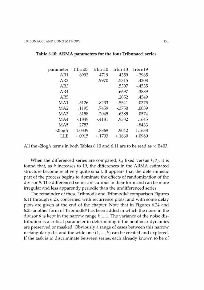
TRIBONACCI AND LONG MEMORY 151
Table 6.10: ARMA parameters for the four Tribonacci series
parameter Trbrn07 Trbrn10 Trbrn13 Trbrn19AR1 .6992 .4719 .4359 -.2965AR2 -.9970 -.5315 -.4208AR3 .5307 -.4535AR4 -.6697 -.3889AR5 .2052 .4549
MA1 -.5126 -.8233 -.5541 .0375MA2 .1195 .7459 -.3750 .0039MA3 .3158 -.2045 -.6385 .0574MA4 -.1849 -.4181 .9332 .1645MA5 .2753 -.8433
-2logΛ 1.0339 .8869 .9042 1.1638LLE +.0915 +.1703 +.1660 +.0980
All the -2logΛ terms in both Tables 6.10 and 6.11 are to be read as × E+03.
When the differenced series are compared, kd fixed versus ktθd, it isfound that, as k increases to 19, the differences in the ARMA estimatedstructure become relatively quite small. It appears that the deterministicpart of the process begins to dominate the effects of randomization of thedivisor θ. The differenced series are curious in their form and can be moreirregular and less apparently periodic than the undifferenced series.
The remainder of these Tribmodk and Tribmodkθ comparison Figures6.11 through 6.25, concerned with recurrence plots, and with some delayplots are given at the end of the chapter. Note that in Figures 6.24 and6.25 another form of Tribmodkθ has been added in which the noise in thedivisor θ is kept in the narrow range k ± 1. The variance of the noise dis-tribution is a critical parameter in determining if the nonlinear dynamicsare preserved or masked. Obviously a range of cases between this narrowrectangular p.d.f. and the wide one (1, ..., k) can be created and explored.If the task is to discriminate between series, each already known to be of

152 INFORMATIVE PSYCHOMETRIC FILTERS
Table 6.11: ARMA parameters with differencing at level k
parameter Trbrn07 Trbrn10 Trbrn13 Trbrn19AR1 .1738 1.7685 -.2762 -.5641AR2 -.0688 -.9417 -.0947 -1.3903AR3 -.5756 .1333 -.8412AR4 .5559 -.5687 -.7107AR5 -.6851 -.5675
MA1 -.3206 -2.0710 .0448 .2976MA2 -.7266 1.5726 -.6052 .9995MA3 .6417 -.3288 -.6367MA4 -.0946 .7369MA5 -.4999 .5236
-2logΛ .7399 1.0603 .8688 1.1270
The following series of graphs summarise pictorially the qualita-tive features which vary with the choice of the parameter k. Inthese cases, k is a selective filter and, to match real data prop-erties and exploration over the whole field of k and θ, solu-tions would be needed. The same selected values of k have beenused, prime numbers were chosen to block factorization effects.
————————————————-
the Tribmodk family, with k as the variable, it may be regarded as as esti-mation problem and not an identification problem.
Discussion
As remarked, this part of the study arose out of reconsideration of experi-ments in which it was asked if subjects could serially extrapolate a chaotictrajectory. The answer appears to be that they could not strictly do that, butthat they could do something which preserved some qualitative features,such as quasi-periodicity or anti-persistence, as quantified by the Hurst in-

TRIBONACCI AND LONG MEMORY 153
Figure 6.3: Tribmodkθ 07 series, 1,200
Figure 6.4: Tribmodkθ 07 differenced at 07 series

154 INFORMATIVE PSYCHOMETRIC FILTERS
Figure 6.5: Tribmodkθ k=10 series, 1,200
Figure 6.6: Tribmodkθ k=10 series, differenced at 10

TRIBONACCI AND LONG MEMORY 155
Figure 6.7: Tribmodkθ k=13 series, 1,200
Figure 6.8: Tribmodkθ k=13 series, differenced at 13
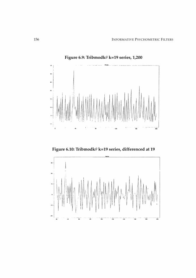
156 INFORMATIVE PSYCHOMETRIC FILTERS
Figure 6.9: Tribmodkθ k=19 series, 1,200
Figure 6.10: Tribmodkθ k=19 series, differenced at 19

TRIBONACCI AND LONG MEMORY 157
dex. It is easier to extrapolate locally from a chaotic series generated fromthe logistic map than from a random series.
The Tribmodkθ series created here might be thought of as a nonlinearydynamic repeatedly disrupted by transients; in this sense it has some eco-logical validity. That argument has been appealed to by Gregson (1995)in the context of nonlinear psychophysics but using the Γ recursion. Thepoint being made here is that using the logistic attractor after reaching sta-bility on the invariant manifold is an extreme form of stability. Even so,trajectories from stationary nonlinear dynamics can have subseries whichare qualitatively identifiably different from the rest of the series (Warren,Bashford, Colley & Brubaker, 2001); if these are what are presented as thestimulus series the results could hardly be the same as from some othersubseries from the same trajectory, though the subseries themselves maybe identifiable by the observer.
Four studies that have focussed on the serial extrapolation problemare by Neuringer and Voss (1993), Metzger (1994), Smithson (1997) andWard and West (1998). These all used the logistic function with the gainconstant set near 4 to produce a trajectory that was stable. Heath (2002),however, used a Henon attractor to generate a discretized trajectory. Thedetails about what subjects were asked to do, in terms of length of stim-ulus series, length of extrapolation, comparison with random series, andfeedback provided or withheld, differ between studies. Heath importantlyshowed that some subjects could discriminate (in terms of very local serialextrapolation) a chaotic series from one with the same spectral density thatwas not chaotic. The mode of response and the precision of responses re-quired also varied. The analysis of results was in some cases presented asthe lag-one plot xi 7→ x(i+1), which takes a very simple form for the logis-tic function. Metzger showed that if precision of response is relaxed then asimple rule, that can be learnt from inspection of the stimulus series, willapproximate the lag-one delay plot. No such simple rule does generallyexist, and in some of the Tribmodk and Tribmodkθ examples used here itis not in such a tidy form. In short, the logistic function is not a valid basisfor making assertions about chaotic trajectories in general.
But Metzger’s demonstration raises another important point; she

158 INFORMATIVE PSYCHOMETRIC FILTERS
showed that the delay plot is roughly approximated if the observer usesa small, and thus finite, set of rules of the form ”if j occurs then follow itby k”. This gives a series of lumps which lie roughly on the continuouscurve of the logistic delay plot, a parabola for the gain parameter valueselected. But such a set of rules are the cells of a transition probability ma-trix; if that matrix is ergodic and complete, and the mapping is from t tot+ 1, so no diagonal cells are absorbing states, then it may generate quasi-periodic cycles. In short, it resembles a Markov process and it may be anti-persistent. It is thus not incompatible with Smithson’s later analysis. Thequestion is, as originally put in these series extrapolation tasks, can the ex-trapolation from a chaotic trajectory be itself chaotic? The answer, if sub-jects are doing what Metzger identified, is no, because (Martelli, 1992, p.206) ”the conditions which qualify a system as chaotic require the presenceof aperiodic orbits, but are not met by any dynamical system governed bya q × q matrix M .” To explore this point further here we need Markovianapproximations to the Tribmodkθ series, for an arbitrary number of statesq. These and the terminal state vectors at ∞ are shown in the table, allassuming an equiprobable starting (rectangular) vector. The assumptionis that five states are sufficient to represent the upper limit on memorystorage that a subject would use to construct rough transition rules. Thepatterns suggest that Tribmod19θ would defeat a subject attempting ex-trapolation on that basis.
Human Predictive Capacities
As noted, a number of studies have addressed the question as to whetherthe human subject can serially extrapolate a series that is either randomor chaotic and not, therefore, strictly periodic or stationary. We know thatobservers have difficulty in recognizing what is a random sequence andattribute to local features evidence of non-randomness that is not statisti-cally valid. But recognition and production of series require different abil-ities that are not tightly coupled: I can tell often that music is by Mozartand not by Brahms, but I can play neither.

TRIBONACCI AND LONG MEMORY 159
Table 6.12: Markovian representation with 5 statesTransition probability matrices for Tribmodkθ series
d1 d2 d3 d4 d5 ∞Tribmod07θ
.82 .15 .02 .01 .00 .736
.59 .28 .10 .00 .03 .190
.33 .25 .33 .00 .08 .059
.00 1.00 .00 .00 .00 .005
.00 .50 .50 .00 .00 .010Tribmod10θ
.55 .24 .21 .01 .00 .558
.54 .24 .14 .04 .04 .246
.62 .29 .09 .00 .00 .171
.67 .33 .00 .00 .00 .015
.50 .00 .50 .00 .00 .010Tribmod13θ
.47 .15 .20 .15 .04 .488
.46 .22 .12 .17 .02 .201
.58 .29 .06 .06 .00 .156
.46 .31 .15 .08 .00 .131
.60 .00 .20 .20 .00 .024Tribmod19θ
.65 .00 .00 .15 .20 .563
.76 .24 .00 .00 .00 .143
.00 1.00 .00 .00 .00 .035
.32 .60 .08 .00 .00 .122
.37 .00 .19 .26 .19 .137

160 INFORMATIVE PSYCHOMETRIC FILTERS
There is a little-known historical precursor to such experiments, inwhich Whitfield (1950)5 asked subjects to respond to an imaginary ques-tionnaire, to which only their responses were recorded; the questions wereprivate inventions of the subject and not revealed. He found that the statis-tical structure of their response sequences, made in yes-no or rating scalefashion, changed with the length of the questionnaire. In modern parlance,they moved onto an attractor over time. The important thing about this ne-glected study is that there was nowhere any mention of randomness, butthe subjects were free to run onto an attractor of their own devising anddid so. The results showed that the series were autocorrelated, to somedegree, and unbalanced in terms of the proportion of ’yes’ and ’no’ re-sponses to an imaginary questionnaire which only allowed for binary re-sponses. There were also warm-up effects. These features match what isreported in random series production experiments; it suggests that callinga series random may be irrelevant, but that the human respondent doesinvoluntarily converge onto a noisy attractor. Call that attractor Q, and itstrajectories on its manifold the set t(Q).
Serial extrapolation without feedback has some common features withthe imaginary questionnaire, what subjects do after they have only theirmemory to rely on for extrapolating a quasi-periodic series, (largest Lya-punov exponent positive and exponentially decaying local predictability)is to move to an attractor with intrinsic instability. Even for extrapolatingthe simplest sinusoid, as in motor skills, there will be second-order de-partures from a limit cycle and response sequences that locally return tothe deterministic trajectory, such as overshooting or delays. Such patternshave been studied from the standpoint of ODEs of oscillations (Hale, 1963;Hoppensteadt, 1979).
If the stimulus series is presented continuously in parallel with the re-sponse series, then it may take on the role of a forcing function, not nec-essarily at a conscious level. This requires a different method of analysis(Gregson and& Leahan, 2003).
Suppose that the original stimulus series is generated by a determinis-
5 This work was done at University College, London, at the time I was a student.

TRIBONACCI AND LONG MEMORY 161
tic attractor A and that the subject has in her own response repertoire A∗where A∗ has two properties, it is contaminated with stochastic noise andit is in some sense near to A. In fact, what we can only observe as subject,but not as experimenter, are trajectory samples, τ(A) and τ(A∗).
Various questions then arise: if, instead of A, we present A∗, does thismake the serial extrapolation task easier or harder? To put it another way,if the subject already has both B∗ and A∗, does the presence of A∗ make iteasier to avoid using a mismatch B∗? What constitutes a match or mis-match for the task is in terms of trajectories τ(A) ' τ(B∗), not directmatching, though some attempts have been made subsequently to matchby Poincare diagrams. It is assumed that a subject can not produce a purelydeterministic nonlinear trajectory by making motor or verbal responsesand it is doubtful if a linear process can be produced without some errortolerance.
The family Tribmodk with variable k produces trajectories that do notsimply resemble one another; from comparing some samples the subjectcannot readily see that only one parameter is involved in generating thediversity of patterns, re-exploration of a family of perceptually similar pat-terns is not necessarily an optimum search strategy to find a valid serialextrapolation sequence. If only a family B∗ exists, then the subject seekswithin that family to find a close match to the presented A∗ by varyingsome parameters in a subset of B∗. As soon as noise is admitted, thedistinction is between ∃A ∩ B which may not be a condition that could besatisfied, and ∃A∗∩B∗ butA∩B = ∅which can be satisfied rather triviallyif there is no upper bound on the noise variance.
There is yet another way of conceptualising the conflict between twotrajectories: as an invasion by the stimulus attractor of the attractors al-ready dynamically resident within the observer. By an analogy with eco-logical models (Geritz, Gyllenberg, Jacobs & Parvinen, 2002), the stimulusseries is a mutant invasion, which may be absorbed, continue in parallel,or overtake the system. Such replacement of the initial dynamics is im-plausible in the context of the serial extrapolation experiments, they arenot like learning to play a Beethoven sonata that is long, complicated andremembered.

162 INFORMATIVE PSYCHOMETRIC FILTERS
What subjects can actually do with simpler oscillating series as a track-ing rather than an extrapolation task has been surveyed by Large andJones (1999). If the subject has alternative choices of series to employ, thenit becomes a sort of discrimination task for quasi-periodic series; Mein-hardt (2002, p. 143) observes in an analogous context that ”discriminationlearning can be understood as a higher level process of gradual refinementof code selection out of a rich code base provided by lower level stages”.The problem is that no lower level stage may lead by revision to an attrac-tor that is synonymous in some sense with a chaotic trajectory.
There have been numerous attempts in statistical and physical the-ory to identify the dynamics of nonstationary time series for example,by Machens (2002) in physics and Fuentes (2002) in spatial processes butthese are useless for the short series of psychological data, though sugges-tively they may employ information measures, or interesting convolutionsof stationary processes that become nonstationary in the long run.
In formal terms, the problem and some of the observable results forTribmodkθ, θ ∼ rect[k ± 1] here are related to the theory of stability underperiodic disturbances (Hoppensteadt, 2000, p.106); under some conditionsthe trajectories of the perturbed system lie sufficiently close to those of theunperturbed system. The examination of the recurrence and delay plotsgives some qualitative idea of what noisy disturbances are tolerable in thestimulus series.
It is known, from analyses of the more standard nonlinear attractor dy-namics (Logistic, Henon, etc) that a small introduction of stochastic noisedoes not perturb the closure of limit cycles, but a larger noise level willeventually destroy the attractor structure (Kapitaniak, 1990). A determin-istic trajectory is replaced by a noisy orbit, which is what we have donehere with Tribmodk. But if the noise is slight, the largest Lyapunov expo-nent remains positive and its fluctuations are smoothed out. The separa-tion of trajectories in chaotic dynamics (associated with the positive LLE)is accompanied by noise which is well-known in diffusive processes. Inthis context, compare the 2D delay plots from Tribmodk and Tribmodkθwith θ ∼ rect[k ± 1], and with Tribmodkθ 1 ≤ θ ≤ k. The narrow bandnoise appears to clarify the delay plot structure, the wide band noise de-

TRIBONACCI AND LONG MEMORY 163
stroys it.There are yet more difficulties, in that if we did have a long enough
response series to evaluate its properties it could not with certainty beconcluded that it was chaotic, even if the original stimulus series was it-self chaotic and the two appeared to match. Hoppensteadt (op cit., p. 200)notes that some functions of a slow almost periodic form can be indis-tinguishable from chaotic series in practice, say chaotic series that have apower spectrum supported by an interval of frequencies. So comparingthe stimulus series and the extrapolating response series by comparisonof Fourier spectra may be an inappropriate test.
The psychological question that remains is what, if anything, in humanperformance resembles the mixed deterministic-stochastic evolutions syn-thetically generated here when cognitive tasks are repetitively performed?If serial extrapolation is induced from a mixed system and mixed systemsare characteristic of human performance, then the problem is to measurethe disparity (or match) in the dynamic structure of two mixed systemsand to find measures of nearness of the two systems from relatively shorttime series. The approach illustrated here creates reference patterns fromTribmodk and Tribmodktθd and would then require that data from realhuman extrapolative behaviour was analysed in exactly the same way.There is no known single sufficient statistic to characterise the evolution ofmixed nonstationary processes and no reason to think that one would ex-ist, though attempts have been made to devise such a measure on a struc-tural equation which has mixed dynamics (Kauffman & Sabelli, 1998).
Conclusions
In the serial extrapolation task there are a number of different mechanismsinvolved:
(1) The local trajectory from a known but — to the subject — unspecifiedattractor A,

164 INFORMATIVE PSYCHOMETRIC FILTERS
(2) Some attractor B∗ (or one of a set of such attractors between whichswitching might spontaneously occur) in the subject that is per-turbed from its manifold by transients from other attractors,
(3) The storage of A as A∗ in short-term memory,
(4) a modification or replacement of B∗ by A∗ where these two share lo-cally some coarse trajectory properties, as a sort of learning. It is thisstage where something like a Markovian process may be substituted
(5) a drift back to the reinstatement of B∗ as the resting state of the ob-server’s system dynamics.
It is (4) that presents problems, for various empirical and mathematicalreasons (Buescu, 1997; Wiggins, 1992; Hoppensteadt, 2000). The operationof one attractor on another can be induced by a forcing function, by a tran-sition over a heteroclinic orbit, or by more exotic processes that are notdemonstrable except in simulations with very long running times6. Thereis no way with short data series that resolution of these ambiguities can besolved. The few properties of the observed time series that have been usedto match the stimulus and extrapolation response series are not specifi-cally characteristic of nonlinear dynamics, and indices that might be ofuse, such as LLLE, are not computable on short series, indices such as ESfthat are computable are not fixed scalars for most nonlinear evolutions,even under stationarity in the sense of being on an invariant manifold.
Note
The employment and meaning of the Schwarzian derivative (Schwarz,1868) in nonlinear psychophysics was noted previously (Gregson, 1988,p. 27). It measures a property sometimes called ”expansiveness”. In one
6 Concepts such as riddled basins or distinctions between different forms of attractor havefound no use in attempts so far to apply chaos theory to psychological processes, as distinctfrom physiological or ecological modelling.

TRIBONACCI AND LONG MEMORY 165
dimension, it is a natural measure of non-projectivity of a transformationf (Sullivan, 1983, p. 727).
There are fundamental differences between the information in a fre-quency analysis and that in the ESf representation7. The frequency do-main representation, by Fourier’s theorem, linearly partitions the seriesinto parts of an infinite sum
f(x) :=∞∑i=1
F (αi, πi, θi) [6.11]
where α is amplitude, π is periodicity of a sinusoidal component F , andθ is phase. The series is truncated to sufficient terms to give an approx-imation when the data series is of finite length. The α information is re-moved by [6.1], the phase θ is not considered at all and the periodicity πis effectively partitioned into slow and fast components so that the infor-mation in the fast components dominates the construction of Tribmodk.The slow dynamics function as a carrier and, if they are sinusoidal, thentheir second and later absolute differences vanish and for the slow partsESf → 0. The representation of nonlinear trajectories as being a conse-quence of slow/fast psychological dynamics has been found informative.It is also noteworthy that approximate entropy measures, such as ESf ,have found significant diagnostic use for dealing with local transientsin EEG records in anaesthesiology (Bruhn, Ropcke, Rehberg, Bouillion &Hoeft, 2000).
7 The shift from derivatives of a continuous function to discontinuous sequences is notinnovative; see Chalice (2001) on the analogues of differentiation in discrete sequencesand Sandefur (1990) for applications in dynamics

166 INFORMATIVE PSYCHOMETRIC FILTERS
Figures 6.11 and 6.12: Recurrence plots for Tribmod 07 and Tribmod 07θ
The effect of θ randomization is to destroy the broken 7 periodicity. Notethe initial unstable period before the process runs onto an attractor on theinvariant manifold.

TRIBONACCI AND LONG MEMORY 167
Figures 6.13 and 6.14: Recurrence plots for Tribmod 10 and Tribmod 10θ
There is a suggestion of non-stationarity here, but otherwise it is not inter-esting. Perhaps this is because here k is not a prime number.

168 INFORMATIVE PSYCHOMETRIC FILTERS
Figures 6.15 and 6.16: Recurrence plots for Tribmodk 13 and Tribmod 13θ
This is perhaps the most curious pattern emerging in the dynamics. Theprocess jumps between three phases, two of which are strongly periodic,suggesting two or more attractors.

TRIBONACCI AND LONG MEMORY 169
Figures 6.17 and 6.18: Recurrence plots for Tribmod 19 and Tribmod 19θ
The effect of θ randomization is to destroy both the broken and the contin-uous 19 periodicity. The initial period of instability is much shorter here.

170 INFORMATIVE PSYCHOMETRIC FILTERS
Figure 6.19: Recurrence plot with narrow noise on k, k = 7 and 10
Figure 6.20: Recurrence plot with narrow noise on k, k = 7 and 10

TRIBONACCI AND LONG MEMORY 171
Figure 6.21: Recurrence plot with narrow noise on k, k = 13 and 19
Figure 6.22: Recurrence plot with narrow noise on k, k = 13 and 19

172 INFORMATIVE PSYCHOMETRIC FILTERS
Figure 6.23: 2-d Delay plot for Tribmodk
Figure 6.24: 2-d Delay plot for Tribmodkθ, k=13

TRIBONACCI AND LONG MEMORY 173
Figure 6.25: 2-d Delay plot for Tribmodkθ, θ ∼ rect[k ± 1]
Postscript on the Figures
The marked diversity of the recurrence and delay plots induced by smallchanges in the parameters is not unique to the Tribonacci series and can beilluminated by recent discussions of the problem of defining exactly whatchaotic means. The most-frequently quoted definitions or empirical testsfor the presence of chaos include sensitivity to initial conditions and pos-itivity of the largest Lyapunov exponent, though neither are strictly nec-essary. Sobottka and de Oliveira (2006) draw a distinction between peri-odicity and eventual periodicity, trajectories that begin aperiodicially andonly after evolution become observably periodic are a property of chaoticdynamics, so recurrence plots that appear random in early iterations andthen periodic are to be expected.Another feature that Yao, Yu, Essex and Davison (2006) consider funda-mental and a definitional property is mode competition, chaotic attractorscreate at least two internal and competing modes. These may be revealedin a frequency analysis, and in unusual patterns in delay plots.


Chapter 7
Rescorla’s Theory ofConditioning
Rescorla and Wagner (1972) published an influential model of classicalconditioning, which has been further refined by Rescorla (2001), introduc-ing as necessary an ogival or cubic function which departs from its originallinearity. The question of interest is whether this revised model could besubsumed as a special case of nonlinear psychophysical dynamics. Theoriginal model, being linear and deterministic, was widely studied andmodified in various ways to try and incorporate stochastic ideas and thuscope with the probabilistic nature of competing response behaviour andresponse measures (Frey & Sears, 1978; Hanson & Timberlake, 1983).
Alternative models for interaction effects between different cues inmaking causal judgements have evolved that vary both in their structureand the number of their free parameters, as well as in prior assumptionsabout what entities may be present in a decision situation. White (2005)gives a review and it is known that effects can be predicted by modelsbetter for this purpose than Rescorla’s. White’s algebra is basically builtfrom linear weighted sums of dimensional components and is extended tocover 24 different conditions for combining evidence. He contrasts it withsome Bayesian nets used to model decisions made by children (Gopnik,

176 INFORMATIVE PSYCHOMETRIC FILTERS
Sobel, Schulz, and Glymour, 2001). We will not here go beyond consider-ing the Rescorla algebra. Its use in causal learning is reviewed briefly atthe end of this chapter.
We will keep Rescorla’s notation for his model throughout:For a single stimulus
∆pn = β(λ− pn) [7.1]
where β is the learning rate parameter, pn is the probability of a responseon trial n, and λ is the asymptote of learning. The complications beginwhen compound stimuli, made up of two or more components, are used.
The model is now expressed in terms of Vi, which is the strength ofassociation to stimulus i. V may be positive or negative and is thus not aprobability. The compound stimulus is called AX , and VAX is the strengthof association of the compound stimulus. The linear assumption is, then,that
VAX = VA + VX [7.2]
which appears from more recent data to be false. When a stimulus com-pound was followed by a US, the changes in the strength of each of thecomponents A and X were taken to be a function of VAX . This was notedto be an important departure from linearity (Rescorla & Wagner, 1972, p.76), but different from that in [7.2].
When a compound AX is followed by US1 then
∆VA = αAβ1(λ1 − VAX) [7.3]
and∆VX = αXβ1(λ1 − VAX). [7.4]
where 0 ≤ α, β ≤ 1. The α are scalar weights. If a different US2 is em-ployed, then the suffices 1 are replaced by 2 in all cases in [7.3] and [7.4].It is assumed that λ is a function of the magnitude of the US. There aresome vaguenesses or, to be more charitable, a lack of formal specificationin the model concerning the boundedness of λ and the V s. A monotonicmapping of V onto response probabilities was assumed.

RESCORLA’S THEORY OF CONDITIONING 177
It follows that, when both VA and VX begin conditioning at zero, thatafter any large number of conditioning trials with AX reinforced
VX =αX
αA + αXVAX [7.5]
which resembles Luce’s version of Individual Choice Behaviour (1959),now known to be in general false.
Extension to Discrimination Learning
Suppose that in a series of trials where AX and BX are mixed randomly,AX is always followed by reinforcement and BX is always followed bynonreinforcement, to induce a discrimination between A and B. Here Xcan be thought of as a background or as contextual cues.
∆VA = αAβ1(λ1 − VAX), [7.6]∆VX = αXβ1(λ1 − VAX) [7.7]
where AX is reinforced, and
∆VB = αBβ2(λ2 − VBX), [7.8]∆VX = αXβ2(λ2 − VBX) [7.9]
where BX is nonreinforced. Together, [7.6, 7.9] is a nine-parameter model;simplifying assumptions by setting all αs = 1.0 and βs = 0.5, and V s zeroprior to the first learning trial were made. The main point of interest is thatAX increases monotonically to an upper asymptote, butBX can variouslyrise and then fall, or fall from the onset of learning. Heath (1979) foundthe linear model inadequate and augmented it using stochastic decisionprocesses.
Various probabilistic schedules of reinforcement are used in condition-ing, and predictions incorporating π, the reinforcement probability on atrial, are derived. Consequentially, π is also the proportion of reinforced

178 INFORMATIVE PSYCHOMETRIC FILTERS
trials in a closed sequence. The asymptotic value of partially reinforced(i.e. π ' 0.5 for each compound stimulus) VAX , VBX is
Vasympt =πβ1λ1 − (π − 1)β2λ2
πβ1 − (π − 1)β2[7.10]
anf if λ1 = 1.0, λ2 = 0 and π = 0.5 then
Vasympt =β1
β1 + β2[7.11]
Rescorla and Wagner derived a diversity of expressions for asymptoticbehaviours under assumptions about parameter values and using the lin-earity assumptions VAX = VA + VX and VBX = VB + VX . An attempt tocircumvent criticisms of the linearity assumption was suggested by treat-ing the stimuli involved as sets VAX , VBX , VABX because VA∩VB 6= 0. ThenVABX → λ1 and VAX → λ2 and so for VBX , so that VX → (2λ2 − λ1), withVA, VB → (λ1 − λ2).
Those details constitute a sufficiency for considering if a parallel withΓ models in NPD is viable.
Structural Analogies
The conditioning theory is essentially about short trajectories leading toasymptotic values where the asymptotes are relative response probabili-ties. In a sense, it is about the orbits of the attractor manifold of the dy-namics, but the model’s only dynamical equations are [7.1, 7.3, 7.4]. Thedata and theory in the source papers do not usually show confidence lim-its on predictions or data, although these could be presumably be derivedwith ancillary assumptions about binomial distributions on the pn.
The entry points for comparison are the equations for two-componentmixtures in each theory, in conditioning [7.3, 7.4], and in NPD (Gregson,1992, p. 24, eqns [2.19, 2.20]) for two continua h, i, (where i =
√−1 when
it is a multiplier and not a suffix)

RESCORLA’S THEORY OF CONDITIONING 179
Yh(j+1) = −ah · (Y ∗hj − 1)(Y ∗
hj − iλh · (ai)−1)(Y ∗hj + iλh · (ai)−1) [7.12]
Yi(j+1) = −ai · (Y ∗ij − 1)(Y ∗
ij − iλi · (ah)−1)(Y ∗ij + iλi · (ah)−1) [7.13]
Both models are written in difference equation form and both can inducelocal transient nonmonotonic trajectories in their dependent variables, thecomparisons would have to be with V s in [7.1, 7.3, 7.4] and Y (Re,Im) in[7.12, 7.13]. What is expressed as two stimuli, A,B, and a background, X ,in pseudodiscrimination experiments is expressed as two complex vari-ables, Y (Re,Im), with shared Y (Im) in 2D NPD Case 2 theory. The fun-damental difference in the objectives of the two theories is that one waswritten for learning and the other for sensation. The possible comparisonarises when responses to mixtures are mediated by nonlinear interactionsbetween continua.
Parameter ComparisonsConditioning Psychophysics Meaning
pn [Y (Re)] response probabilityβ [a] learning rateα [e] weight on βπ [Y (Im)] reinforcement probability
λ1, λ2 asymptotes on VVA [Y (Re)] associative strength of A
VAX [Y (Re,Im)] strength of A with noise XVAB strength of mixed output AB
[β1, β2] a1, a2 gains on each dimension[a] e sensitivity
[VA] 0 < Y (Re)< 1 observable output (response)[π] Y (Im) internal activity
[VABX ] λ cross-couplingη delay time

180 INFORMATIVE PSYCHOMETRIC FILTERS
Note in the table that λmeans an asymptote in conditioning theory, butmeans a cross-coupling in NPD. The two meanings are quite different, butthe symbolism has been retained, so that reference to the original sourcescan be made simpler. We are going to drop the asymptote idea later inrevising NPD to incorporate some sort of conditioning process.
To compare the two models, the parameters have to be matched, if theyfunctionally correspond. Such correspondence does not necessarily haveto exist for all parameters; that is, their role within the model may be giventhe same meaning, but obviously their numerical values do not match. AsNPD is written as a difference equation, [7.1] may be revised to facilitatethe explication and comparison of model differences as
Vn+1 = (1− β∗)λ+ β∗Vn [7.14]
where β∗ = 1−β. Equation [7.14] shows that the model is a linear weightedcompromise of a postulated asymptote and the present value of V . Thereis no need to put an asymptote into Γ [7.12,7.13] because that recursion isself-limiting in Y (Re) within its attractor basin of stability. In the table ofParameter Comparisons near-functional equivalences have been indicatedin [..]; such equivalences are not necessarily symmetrical.
The Γ recursions are the basis of the observable map MΓ := a 7→ Y (Re)and the conditioning of the map Mcond := π 7→ V , as a and π are underexperimenter control and functions of Y (Re) and V are treated as responsescale values. As MΓ is the result of a complex cubic polynomial function,it is ogival. Rescorla (2001) has now revised Mcond to be ogival becausea linear map does not fit data. One may say that end effects at zero ornear asymptote exhibit nonlinearities; this is a weak convergence of thetwo models. The question we now explore is: can the conditioning modelbe rewritten as a special case of NPD? It could be argued, on the basisof a sort of biological economy, that the same brain has to support thesequential dynamics of the domains of activity, sensation and learning.Any model which is linear in its details can be treated as a local subregionof the dynamics of a more general nonlinear model on the principle ofpiecewise linearization.

RESCORLA’S THEORY OF CONDITIONING 181
The entry point of the argument is to note that ∆Y = f(e, Y (Im)) and∆V = g(α, β) are bivariate operator equations f, g respectively in the twomodels that control rates of change of their dependent variables. But inconditioning there is an extra variable π, a variable reinforcement param-eter, that has no counterpart in sensation. This is equivalent dynamicallyto having a nonstationary feedback loop added to the recursion. To recallthe distinctions of the introduction, we move from U to C time series.
A simple heuristic way to parallel the reinforcement parameter in anaugmented Γ is to make e in one-dimensional NPD a function of an exter-nal schedule Sj .Then
Γ := Yj+1 = −a · (Yj − 1)(Yj − i · f(Sj))(Y + i · f(Sj)), i =√−1 [7.15]
The time series generated by [7.15] is
Yj+1 = f(a, Sj) [7.16]
and [7.14] with π incorporated as in [10] is
Vn+1 = (1− β′)λ+ β′Vn [7.17]
where now β′ = (1− πβ).
The suggested necessary modification of [7.2] which Rescorla (2001, p.64) considers for compound stimuli is
VAAB = f(VA) + f(VB) [7.18]
and now this f is sigmoidal, so it would resemble MΓ1.
1 The theory variant called ΓV 1 in Gregson (1988) uses ej = f(∆1aj), which means thatresponse sensitivity is a function of a local rate of change of stimulation. This is a sort offeedback, whereas π in [7.10] is not contingent on ∆V . To modify [7.15] to accommodateschedules of reinforcement Sj is therefore not the same as using ΓV 1.

182 INFORMATIVE PSYCHOMETRIC FILTERS
Simulation in 2D NPD
The problem now is to see if variations in the parameter values of 2Γ Case2 equations can produce some of the same time series for reinforced andunreinforced components of a stimulus mixture. This will be attemptedin two stages: first, a purely deterministic treatment of S = f(j) in [7.16],and then a stochastic revision in which the shifts in parameters from trialto trial are probabilistic and not a monotone function of time.
Deterministic model
The qualitative pattern it is desired to reproduce, without any structuralchanges in the 2Γ model, is that in which the reinforced component slowlyrises in output strength with successive reinforcement, but the unrein-forced component first rises a little and then falls off to a low asymptote.This rise and then fall in a component which is to be extinguished is sup-posedly paradoxical for some linear models. It is necessary first to showthat a configuration of 2Γ parameter settings which are not implausible,given the extensive results (Gregson, 1992, 2001) in other sensory (but notlearning) situations can yield the apparent paradox.
The parameters in a 2Γ Case 2 model are set initially asY0(Re, Im)1, Y0(Re, Im)2, a1, a2, λ1, λ2, η. Putting Y0 = (0.5, η) for both di-mensions sets the process as initially stable. η = 10 has been fixed through-out, as response delay is not a variable system parameter being modelled.a1 = 2.4, a2 = 3.6 assumes that when the response to dimension 1 is ini-tially unconditioned then the noise strength a2 is greater. Both the a valuesare left unchanged, as the actual stimuli do not change, only the relativeresponses to them. The only parameters available to represent an alteredsensitivity to stimuli and interaction between stimuli are λ1 and λ2. Con-tinuing reinforcement over a long series J = 1, ..., N of trials thus implieshere that SJ = f(λ1, λ2, J).
After some exploratory analyses, it is found that setting initial valuesλ0,1 = 0.2, and λ0,2 = 1.15, and incrementing on each trial
∆1λ1 = +.04, ∆1λ2 = −.04 [7.19, 7.20]

RESCORLA’S THEORY OF CONDITIONING 183
yields Figures 1 and 2. Bounds on e1, e2 of e1 < .45, e2 > .01 were set2,though these are not hit for e2 in the series until J = 30.
Figure 7.1: Time course over trials J of Y(Re)1; reinforced
Figure 7.2: Time course over trials J of Y(Re)2; extinguished
Figure 1 is an analogy of VA time series and Figure 2 is an analogy ofVX . If an analogy of [7.2] is required then the two curves are summed atany point J . This would here yield an almost flat curve for the mixture un-til a1 dominated, which is implausible unless weighted summation wereto be used.
2 In Case 2 the cross-coupling is effected by making e1 = λ1/a2, and e2 = λ2/a1. It isknown from previous psychophysical results that plausible values of e lie in the range.01 < e < .45.

184 INFORMATIVE PSYCHOMETRIC FILTERS
Stochastic models
Now the increments [7.16, 7.17] in λ1, or 2 are made with associated proba-bilities, which adds another two parameters π1, or 2 to the model, compare[7.10]. There are obviously various ways in which this can be done; one,which creates slight second-order changes to the Figures 7.1 and 7.2, is towrite the random variable κ ∼ RECT (0, 1), and then
for reinforcement: λJ = λJ−1 + κ · .2− .05 [7.19]
for extinction: λJ = λJ−1 − κ · .2 + .05 [7.20]
which produces Figures 7.3 (corresponding to 7.1) and 7.4 (correspondingto 7.2). The shifts to conditioning or extinction now arise sooner and moreabruptly and the reinforcement curve runs to an asymptote.
Figure 7.3: Time course of reinforcement with stochastic perturbation
Figure 7.4: Time course of extinction with stochastic pertubation
Note that the initial rise in the extinction curve still exists. This riseexists if there is an appropriate choice of a combination of all of the pa-rameters a1, a2, λ1 and λ2.

RESCORLA’S THEORY OF CONDITIONING 185
Another much more erratic substitution of a stochastic component onthe λ values is shown, without any commitment to its plausibility. Whenconditioning experiments are run, there is no certain smooth improvementin performance, and local failures or relapses can arise, but unless these arereported in detail without averaging over replications (which is not usual)it it not possible to know if they are faithfully modelled in any simulation.However, the next two figures 7.5 and 7.6 depict what can happen. Theequations corresponding to but replacing [7.19,7.20] are (J = 1, ..., 30)
for reinforcement: λJ = λJ−1 + .04 · J(2.0 · κ− 1.0) [7.21]
for extinction: λJ = λJ−1 − .04 · J(2.0 · κ− 1.0) [7.22]
Figure 7.5: Reinforcement with erratic stochastic effects
Figure 7.6: Extinction with erratic stochastic effects

186 INFORMATIVE PSYCHOMETRIC FILTERS
Higher and Indeterminate Dimensionality
The Rescorla-Wagner model has been used in other contexts than the orig-inal conditioning paradigms for which it was created. One area of interestis the learning and use of causal inference in humans as a topic in develop-mental psychology (Gopnik, Glymour, Sobel, Schulz, Kushnir and Danks,2004). It transpires that the Rescorla-Wagner model can not capture someprocesses of causal inference, but another approach, based on directedacyclic graph theory, can do better. Such graphs are called Bayes nets whencombined with a recursive strategy to choose between various links be-tween nodes. With the subsequent use of Bayes theorem to compute var-ious posterior probabilities associated with different links and subsets ofnodes in the graph. Bayes nets were developed in artificial intelligence asone way of solving what has come to be called the inverse problem (Pearl,1988). This finding about the inadequacy of the Rescorla-Wagner model ispertinent here because, to the extent that the Rescorla-Wagner equationscan be treated as analogous to NPD equations, then those also would failif used without modification as suitable for representing inference judge-ments.
There are, however, some complications: in equations [7.1-7.22] wehave restricted comparisons to what are two-dimensional processes andcausality situations generally involve more terms, so that directed pathslike X → Y may be wrong as failing to reveal that the true situation isX ⊥ Y, Z → Y, Z → Y where ⊥ means causally independent. This islike the situation in statistics where partial correlations and not first-ordercorrelations should be used to reveal psychophysical influences like thosemapped in Chapter 1, in Figure 1.3.
Gopnik et al, (2004,p.6) observe pertinently that
Causation is not just correlation, or contiguity in space, or pri-ority in time or all three. Causal structures rarely just involveone event causing another. Instead, events involve many differ-ent causes interacting in complex ways. A system for recover-ing causal structure has to untangle the relations among those

RESCORLA’S THEORY OF CONDITIONING 187
causes and discount some possible causes in favour of others.
Even if the underlying causal relationship is deterministic, theoccurrence of other causal factors, which may not be observed,will typically make the evidence for the relationship proba-bilistic.
All this is true; the a priori indeterminacy of the number of variables,and hence the dimensionality of the system, is critical and almost alwaysgreater than two, but it is still not sufficient. The Bayes net approach isacyclic, so there are no feedback loops in it, and the assumptions are thatdeterministic and stochastic linkages are all that may prevail; there is noprovision for some of the characteristic features of nonlinear dynamics,including mixes of fast and slow dynamics, which arise naturally in NPDbut not in R-W. White (2005, p. 131) suggests that the RW model can besupplemented by ”an account of within-event associations”, which wouldinvolve more parameters and something like adding fast dynamics. Atthe same time, it is clear that causal learning involves more than bare psy-chophysical mappings, that are necessary but not sufficient.
Both Rescorla-Wagner equations and NPD create trajectories of associ-ation or estimates of causal strength; they involve changes over time andrun asymptotically to equilibria, whereas the Bayes nets need augmenta-tion to do that. Gopnik et al (2004, p.19) show experimentally that there areproblems children can solve, involving what is called ”backward block-ing”, that are outside the scope of causal Rescorla-Wagner models but canbe handled by some Bayes nets. Backward blocking is the situation wherelearners decide if some event is a cause of an effect by using informationwhere the event never appears in conjunction with other trials where itdoes appear. The RW model can be modified by adding axioms that de-crease the association of a cue with an outcome when the outcome occursin the absence of the cue. Also, the RW model requires a prior specificationof the direction of putative causal links, whereas Bayes nets (and humans)can, in some circumstances, decide between X → Y and Y → X . It maybe important that in using nΓ equations we have always that
Cause→ a, Y → Effect,

188 INFORMATIVE PSYCHOMETRIC FILTERS
that is, causal direction is expressed in model structure in a different wayfrom that in RW. If the extension to n×nΓ is used (Gregson, 1995), then thestructure of an n × n matrix of λ coefficients in [7.12, 7.13] is also neededto be solved for. That corresponds to restricting the (0,1) links in a directedBayes net.
At the present state of knowledge, it can be safely asserted that noneof the competing models have universal validity for explaining how andwhat causality inferences are actually made by human subjects. Condi-tioning theory, of which RW is a particular case, does not effectively dealwith human contingency judgements (Shanks, 1985), nor with the role ofassociated implicit stimuli (Miller, Barnet and Grahame, 1995).

Chapter 8
Nonlinearity, Nonstationarityand Concatenation
A comparison of six time series two from pseudo random generation, twofrom convoluted theoretical psychophysics, and two from EEG recordsare compared using a set of four statistics. It is seen that local largestLyapunov exponents, the entropic analogue of the Schwarzian derivative,higher-order kernel matrices, surrogate random tests for confidence limitson parameters and eigenvalues of the dynamics all yield different infor-mation about the local instabilities of the processes. All the time series are,in some way, different from one other.
Only something that appears to be both orderly and disor-derly, regular and irregular, variant and invariant, constant andchanging, stable and unstable, deserves to be called complex.
(Edelman & Tononi (2001, p. 135).
The investigation of unstable quasi-periodic orbits where there is noisepresent and surrogates may be employed has become of increasing inter-est in the study of biological data. Such data include psychophysiologicaltime series such as scalp EEGs (Ding, Ditto, Pecora & Spano, 2001). Therehas also emerged a diversity of methods for looking at nonlinear nonsta-

190 INFORMATIVE PSYCHOMETRIC FILTERS
tionary dynamics in time series, which, however, are only tractable forvery long series. For example, Casdagli (1997) reviews the use of recur-rence plots on series between 5,000 and 60,000 iterations long. The ESfmethods used here were deliberately created to look at very short seriesfrom psychophysical and psychophysiological data sets, where 100 iter-ations under stability is often a practical limit. The general problems ofemploying statistical analyses to discriminate between randomness andchaotic dynamics in time series, particularly in higher dimensionalities,something that is not always possible, are reviewed by Berliner (1992) andcommentators and the valuable role of symbolic dynamics was then al-ready known.
In psychophysiology, the identification of transient nonstationary pat-terns of activity has been explored theoretically as a basis for perceptualand memory processes (Gregson, 1993, 1995; van Leeuwen & Raffone,2001). The idea being pursued is that the dynamics of neural activity haveto be very labile for the brain to be able to learn and to revise rapidly andcontinually its processing of perceptual inputs. In time series terms, this la-bility implies possible nonstationarities and singularities. So, except oververy brief realisations, statistics such as frequency domain spectra or auto-correlations will mask and not reveal singularities as they involve only asmall part of the energy distribution of the process and become masked inany averaging over time. In the particular case of the Fourier transforms,by FFT analyses, if one were to capture the singularities or abrupt jumps,spikes or bursts, as they are variously called in EEGs, then in the limit onewould need an infinite series of frequency terms in the Fourier expansion.The alternative of treating spikes or bursts a priori as outliers is not accept-able in nonlinear dynamics, though outliers can exist as a consequence ofidentifiable exogenous perturbation.
Thom (1975) noted that, in biological data, there may be many localsmall catastrophes in the evolution of a process but, because they are manyand small, their existence would be smoothed out in modelling. However,if one can take short enough series and explore the dynamics within suchepochs, as compared with their smoother neighbouring epochs of similarlength, then the nature of the nonstationarities in the dynamics may be

NONLINEARITY, NONSTATIONARITY AND CONCATENATION 191
clarified. The questions of how and why local anomalous dynamics ariseare tied to the identification of fast/slow dynamics. Van Leeuwen and Raf-fone (2001) come to this problem through considering the activity of thehippocampus as mediated by nonlinear coupled maps. Coupling of fastand slow dynamics can be modelled in various ways: the NPD approach(Gregson, 1998, 1992, 1995) does it with complex variables, and it can alsobe done with real signals riding on slow carrier waves. In psychophysiol-ogy, it is noted that the time scale of sensory processing is much faster thatthat of memory consolidation, though both may run in parallel and mayinvolve neural circuitry via the hippocampus.
Shafer (1994, p.60), discussing the logic of statistical inference writes
We deliberately construct the stochastic story that serves as ourstandard for comparison. We often construct several.....we may(or may not) find a stochastic story in which the performanceof the spectator roughly matches the performance of our fore-caster At no point are we required to think of the forecasterherself or of the phenomenon being forecasted as part of astochastic story.
The fundamental difference here is that trajectories which are notstochastic, or are mixed deterministic and second-order stochastic, maybe used instead of stochastic stories; the matching idea is still the same.
For illustration, two EEG samples are compared with four processes,two of a complicated nonlinear form, and two which are Gaussian i.i.d.series. Thus there are six series, two from real data and four from theoret-ical computations. For each series of 960 steps, there are eight subseries of120 steps. There are four statistical methods used on each subseries, so thetotal study is 6 × 8 × 4 in its full crossed design. This does not imply thatit is amenable meaningfully to Anova.
Statistical Methods
This section recapitulates some previously described uses of methods, tomake the immediate contrast of the methods and their derived indices

192 INFORMATIVE PSYCHOMETRIC FILTERS
more compact, without back reference to the previous chapters.
Lyapunov Exponents
Under some conditions where the diffusion rate of the dynamics of thetime series is nearly zero, the probability distribution of the local largestLyapunov exponent is approximately log-normal (Fujisaka, 1983) and, un-der stricter conditions, the difference between the entropy and the largestLyapunov exponent is approximately constant (Kohmoto, 1988, p. 1349,eqn. 5.9). It is not yet known how well real psychometrical data mightsatisfy these analytical conditions. See Appendix 1 to this chapter for adefinition in terms of Jacobians.
Random Surrogate series
The method of random surrogates to compare a data series with a numberof randomised permutations of the series was introduced by Theiler etal (1992). It is used here in a slightly different manner, though the logic iscomparable. The objective is to match a series in its first two moments, butto remove any sequential dependencies in the surrogates.
Entropic Analogue of the Schwarzian Derivative
This method was introduced by Gregson (2001) and is a parallel of aderivative introduced by Schwarz (1868), but is based on local summa-tions of coarsely scaled series and not on point derivatives of a continuousfunction. The idea of treating a dynamical trajectory from an entropy per-spective is not novel but is well developed (See Sinai, 2000, Chapter 3) andcan be traced back to statistical mechanics in the 19th century.
A series of a real variable y is partitioned into k exhaustive and mu-tually exclusive subranges in the values y it takes, k = 10 is initially suf-ficient. As a condition of the normalisation 0 ≤ y ≤ 1 the end subrangesh = 1, k will initially not be empty. Some or all of the remaining k− 2 sub-ranges may be empty when the dynamics are minimally informative. Call

NONLINEARITY, NONSTATIONARITY AND CONCATENATION 193
the width of one such subrange δ(0) (of y). δ(0) = .1 for the original y butwill almost always be less for ∆m(y), the successive mth absolute differ-ences of the series. This δ is the partitioning constant of the system. Callthe partitioning constant of the range of the mth differences δ(m). In theexamples used here, δ(1) is referred to simply as δ in the tables of results,and all δ(m),m > 0 are set constant = δ(1).
The frequencies of observations lying in one segment δh, h = 1, ..., k isthen nh, and converting to probabilities ph we compute the information inthat subrange. The absolute differences of the rescaled y series are takenputting
∆1(yj) = |yj − yj−1| [8.1]
and further differencing repeats this operation, so that
∆2(yj) = |∆1(yj)−∆1(yj−1)| [8.2]
. This operation can be continued only until all absolute differences arezero. Going only as far as ∆4 is sufficient. Summing over all subrangesgives the total information in the mth differenced distribution as
I(m)h = I(m) =
k∑h=1
phlog2(ph)|m [8.3]
Then by definition the entropic analogue of the Schwarzian derivative,abbreviated to ESf , has the form
ESf :=I(3)
I(1)− 3
2
(I(2)
I(1)
)2
[8.4]
For some strongly chaotic (theoretical variants on Γ) series, ESf is pos-itive in the examples we have seen and becomes increasingly negativeas processes are more stochastic. It has been applied to series from psy-chophysics, EEGs, climate and economics. Its main advantage is that is iscomputable over much shorter time series than the Lyapunov exponents.

194 INFORMATIVE PSYCHOMETRIC FILTERS
Bispectral Kernel Analysis
This method is usually employed in the frequency domain but here a timedomain version is used together with the surrogate tests.
Bispectral analyses are, in fact, third-order kernels of time series. Theyhave been extensively used in anaesthesiology, in the tracking of the evo-lution of EEGs during surgery, following Rampil (1998) and Proakis et al(1992), and are there computed in the frequency domain using FFTs. Theyresemble the kernels used in nonlinear analyses described by Marmamelisand Marmarelis (1978).
If there exists a real discrete zero mean third-order stationary process x,then its third-order moment matrix is defined over a range of lags 1, ...,m,1, ..., n by
R(m,n) := E[x(j) · x(j +m) · x(j + n)] [8.5]
This matrix is skew symmetric, as m,n can be exchanged in the definition.The triangular supradiagonal matrix is sufficient for exploratory purposesand is used in the tables in the form shown. To compute its eigenvalues, itis reflected into the square form and the leading diagonal cells filled withthe average of the off-diagonal cells as an approximation. Its roots will, ingeneral, be a mixture of reals and complex conjugates.
b(1, 2) b(1, 3) b(1, 4) b(1, 5) b(1, 6)b(2, 3) b(2, 4) b(2, 5) b(2, 6)b(3, 4) b(3, 5) b(3, 6)b(4, 5) b(4, 6)b(5, 6)
Compare the usual second-order autocorrelation which is defined as
R(m) := E[x(j) · x(j +m)] [8.6]
over a range of lags 1, ...,m.

NONLINEARITY, NONSTATIONARITY AND CONCATENATION 195
The Time Series Used
(1) A Quasi-Random Gaussian almost-i.i.d. Series
This series was generated, using an algorithm RAN2, by Press et al (1986),with only one linear congruential generator. It is relatively coarse in reso-lution of the numerical values of normal deviates created by subsequentuse of a function GASDEV to transform to Gaussian deviates on the recti-linear deviates RECT(0,1) first generated by RAN2.
Figure 8.1: (1) Gaussian pseudo-random series
(2) A Second Quasi-random almost-i.i.d. Series
This series was also generated from an algorithm by Press et al (1986), thiswas RAN1 employing three linear congruential generators. It is supposedto have finer resolution of the values generated and to show no sensible se-quential correlations. It is assumed that the correlations in question wouldbe first-order of varying lag, as used to create the autocorrelation spectrumof the series. Its periodicity is far beyond the series length used here. Thefunction GASDEV was again used to create a series of random Gaussiandeviates.
(3) Convoluted Gamma Concatenated
Convoluted Gamma trajectories have been previously used for illustration(Gregson, 2000). As they are not phase-locked their short realisations maybe concatenated.
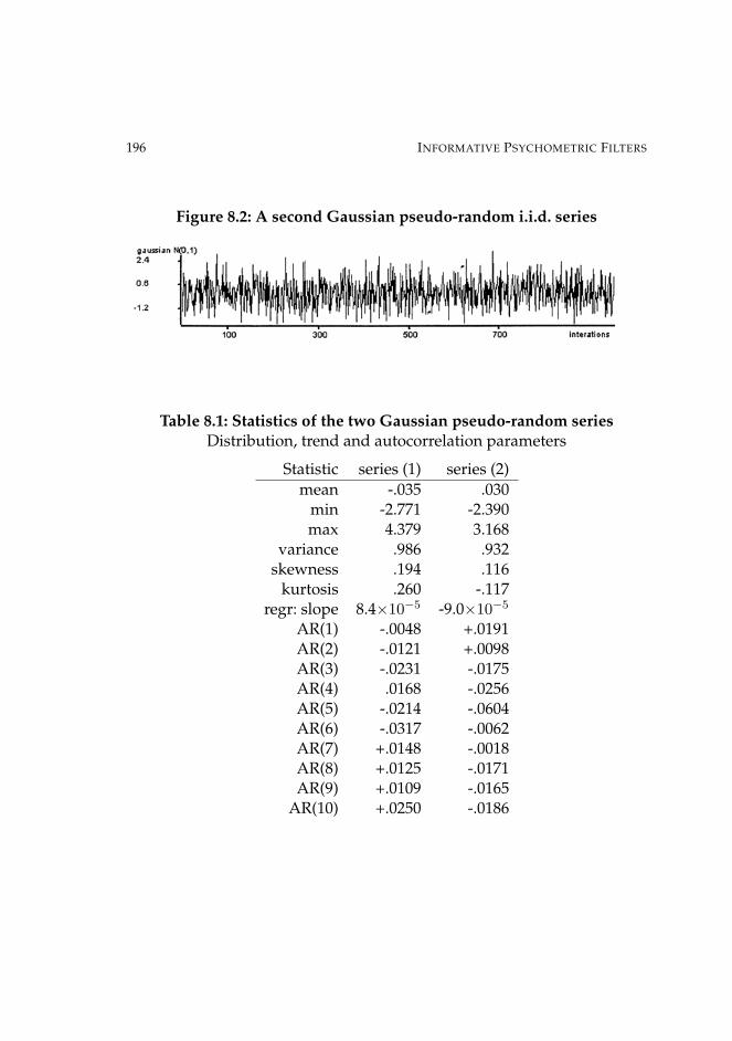
196 INFORMATIVE PSYCHOMETRIC FILTERS
Figure 8.2: A second Gaussian pseudo-random i.i.d. series
Table 8.1: Statistics of the two Gaussian pseudo-random seriesDistribution, trend and autocorrelation parameters
Statistic series (1) series (2)mean -.035 .030
min -2.771 -2.390max 4.379 3.168
variance .986 .932skewness .194 .116
kurtosis .260 -.117regr: slope 8.4×10⁻⁵ -9.0×10⁻⁵
AR(1) -.0048 +.0191AR(2) -.0121 +.0098AR(3) -.0231 -.0175AR(4) .0168 -.0256AR(5) -.0214 -.0604AR(6) -.0317 -.0062AR(7) +.0148 -.0018AR(8) +.0125 -.0171AR(9) +.0109 -.0165
AR(10) +.0250 -.0186

NONLINEARITY, NONSTATIONARITY AND CONCATENATION 197
Figure 8.3: The Raw ConvΓConc series
The first stage is to convolute, by having the parameter a in ΓV 7 avariable, with a random bounded rectangular distribution. That is, for acomplex variable Y (Re, Im)
Γ := YJ,j+1 = −aJ(Yj − 1)(Yj − ie)(Yj + ie), i =√−1, j = 1, ..., η
[8.7]where J (= 1, ..., N) is one cycle in the convolution, and
aJ ∼ α ·RECT (0, 1) + β, aj ∼ i.i.d. [8.8]
where α and β are real scalars. They have to be small and bounded toavoid the process exploding. An additional complication introduced inthis example is that e = c · ∆1(aJ); again, c is bounded. The trajectoryreturned for examination is the polar modulus r value, where
Y (Re, Im) 7→ Y (r, θ) [8.9]
of YJ,η over the range 1, ..., N . Here N = 120 and then eight such serieshave been concatenated. That is to provide a comparison of the patternsfound in some EEG samples (Gregson and Leahan, 2001). This ConvΓConcseries with η = 10 has a curious shape with local erratic high spikes andvery high frequency basal activity. Unless it is known a priori that the se-ries is a convolution of two processes, each of [8.7] and [8.8] is in itselfstationary in its parameters, then externally observed it is sample of a non-linear nonstationary process trajectory. Its largest Lyapunov Exponent L ispositive: LLE = +.0682
The trajectories created from this convolution may be treated as beingon the invariant manifold.
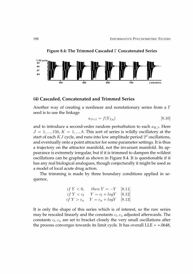
198 INFORMATIVE PSYCHOMETRIC FILTERS
Figure 8.4: The Trimmed Cascaded Γ Concatenated Series
(4) Cascaded, Concatenated and Trimmed Series
Another way of creating a nonlinear and nonstationary series from a Γseed is to use the linkage
aJ+1 = f(YJ,η) [8.10]
and to introduce a second-order random perturbation to each aKJ . HereJ = 1, ..., 150, K = 1, ..., 8. This sort of series is wildly oscillatory at thestart of each KJ cycle, and runs into low amplitude period 2d oscillations,and eventually onto a point attractor for some parameter settings. It is thusa trajectory on the attractor manifold, not the invariant manifold. Its ap-pearance is extremely irregular, but if it is trimmed to dampen the wildestoscillations can be graphed as shown in Figure 8.4. It is questionable if ithas any real biological analogues, though conjecturally it might be used asa model of local acute drug action.
The trimming is made by three boundary conditions applied in se-quence,
if Y < 0, then Y = −Y [8.11]if Y < cl Y = cl + logY [8.12]if Y > cu Y = cu + logY [8.13]
It is only the shape of this series which is of interest, so the raw seriesmay be rescaled linearly and the constants cl, cu adjusted afterwards. Theconstants cl, cu are set to bracket closely the very small oscillations afterthe process converges towards its limit cycle. It has overall LLE = +.0648,

NONLINEARITY, NONSTATIONARITY AND CONCATENATION 199
but the local LLE is not readily computable unless a high-pass filter is usedas well, after which LLE = +.0675
This trajectory lies on the attractor manifold that is deduced from theprocess running onto a limit cycle in the intervals between random per-turbations. Jumping around like that is not necessarily on the attractormanifold, as the Shil’nikov process also has jumps out of and back into aspiral trajectory in the phase space, but lies on the invariant manifold.
(5) EEG under a Control Condition
These data were provided by Kerry Leahan at ANU, drawn from a longseries of recordings of EEGs under a diversity of stimulation conditions.This series was taken from a fifth session, after stabilisation, and there wasno extraneous stimulation used.
(6) EEG under a Relaxation Condition
The series (1) and (2), and (3) and (4), all being theoretical, may be thoughtof as null hypotheses for the two real EEG series (5) and (6). The Gaussianseries are what Shafer called a stochastic story. Alternatively, the Gaus-sian series (1) and (2) may be ignored and the contrast between (3) and(4) which are nonlinear comparison stories in the same manner and (5)and (6) explored to see if the Γ series are in any sense models of the EEGprocesses, though it is not at all probable that they are.
These EEG relax (6) data were recorded from the same study as theprevious series (5), but here there was music played as a relaxing back-ground. In the sense of this study we have aperiodic stimulation of a widespectral form as a weak forcing function, which is not expected to synchro-nise readily with any of the dominant frequencies in the resting EEG. Infact, it is seen to be nearest to a coarser resolution random Gaussian series,with high dimensionality.

200 INFORMATIVE PSYCHOMETRIC FILTERS
Figure 8.5: EEG under a control condition, and its recurrence plot

NONLINEARITY, NONSTATIONARITY AND CONCATENATION 201
Figure 8.6: EEG under a relax condition, and its recurrence plot
Comparison of Higher-order Analyses
Comparative analyses are given for the six series as a whole and for ESf aspartitioned into subseries, at the end of the chapter in Appendix 2.
The tabulations of the ESf and triangular matrices of the kernal ESfvalues for the two concatenated Gamma examples (3) and (4) reveal con-sistent differences, even though both are interpreted as chaotic if the LLEpositivity is taken as a sufficient statistic.

202 INFORMATIVE PSYCHOMETRIC FILTERS
Table 8.2: Summary of LLE and ESf for whole series
series LLE min ESf mean ESf max ESf(1)Gaussian i.i.d +.1386 -.8435 -.6261 -.3680(2)Second Gaussian i.i.d. +.1382 -.6608 -.5809 -.4892(3) CΓC +.0682 -.2822 -.1607 -.0187(4)CCΓT +.0675 +.3987 +.4330 +.4534(5) EEG control +.1268 -.5877 -.4983 -.3501(6) EEG relax +.1086 -.8353 -.6316 -.4543
Even though the LLE values are both positive and not very different nu-merically, the ESf values for both the series and the higher-order kernelterms are very different. For the first case, ConvΓConc (3), the ESf valuesare small and negative for each of the subseries and in subseries 3 and 6 liewithin the surrogate 95% confidence intervals. These are the two subserieswhich have n: 6 and have turning points in the local LLE plots. The actualnumerical values in the triangular matrices are mostly positive and showsome correlation between corresponding cells in the various subseries ma-trices, which suggests that the process is indeed nearer to chaotic than torandom, but shows the nonstationarity which has been observed in theEEG data samples (Gregson and Leahan, 2003). The kernels are, however,very different from those of the EEG series.
The second case, of the trimmed series (4), has a reverse pattern, in thatnow theESf values for the subseries are positive and much larger and thetwo ranges of values do not overlap. None of these ESf values are withintheir random surrogate confidence intervals. The kernel values are mostlynegative, but the n: values are consistently lower. The total series is thus aset of trajectories in the attractor manifold, varying only slightly from onesubseries to the next. That is, there is a periodic but not sinusoidal forcingfunction.
So, here are two cases of nonlinear nonstationary series, but their inter-nal dynamics are very different.

NONLINEARITY, NONSTATIONARITY AND CONCATENATION 203
Another summary description is provided by the relative frequency ofA, W, and B codings for the ESf values for raw subseries in the six tables8.6 to 8.11 in Appendix 2:
Table 8.3: Summary of A,W,B codings for the ESf values
series A W B(1) Gaussian 4 0 4(2) Second Gaussian 5 2 1(3) CΓC 5 2 1(4) CCΓT 8 0 0(5) EEG control 7 1 0(6) EEG relax 1 4 3
Table 8.4 Eigenvalues for submatrices #1 through #4in the EEG Control condition (5)
Eigen Submat # 1 Submat # 2 Submat # 3 Submat # 4[1] -3.5813 -2.7014 -3.9175 -3.7362[2] +.4180 +.2462 -.5021 +.4131[3] -.3201 -.1562 +.4633 -.4002[4] -.1103 -.1120 +.3387 +.2502[5] +.0781 +.0855 -.2041 -.2299[6] -.0421 -.0524 -.0681 -.0164
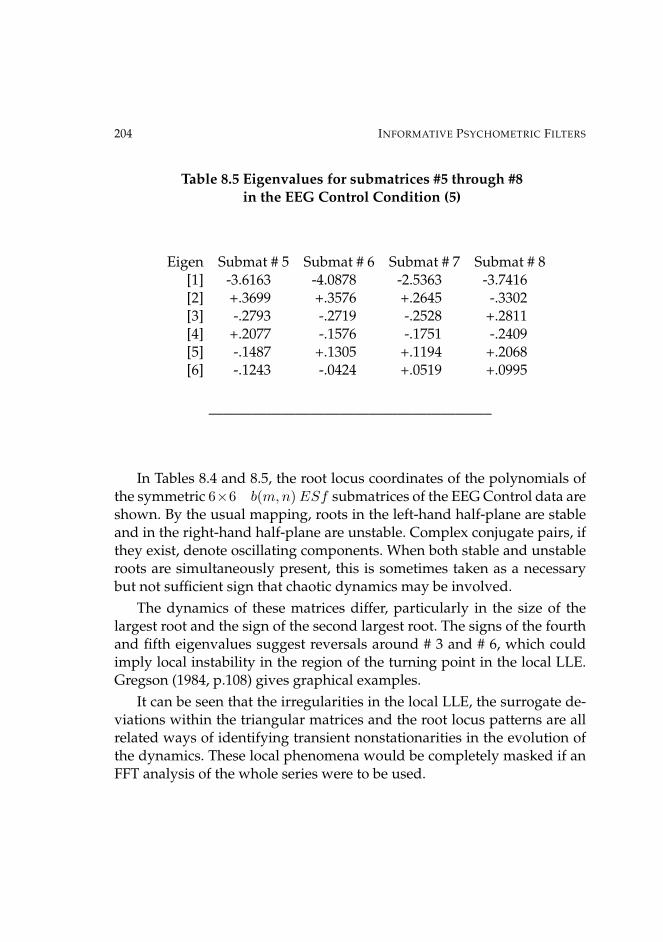
204 INFORMATIVE PSYCHOMETRIC FILTERS
Table 8.5 Eigenvalues for submatrices #5 through #8in the EEG Control Condition (5)
Eigen Submat # 5 Submat # 6 Submat # 7 Submat # 8[1] -3.6163 -4.0878 -2.5363 -3.7416[2] +.3699 +.3576 +.2645 -.3302[3] -.2793 -.2719 -.2528 +.2811[4] +.2077 -.1576 -.1751 -.2409[5] -.1487 +.1305 +.1194 +.2068[6] -.1243 -.0424 +.0519 +.0995
———————————————————–
In Tables 8.4 and 8.5, the root locus coordinates of the polynomials ofthe symmetric 6×6 b(m,n)ESf submatrices of the EEG Control data areshown. By the usual mapping, roots in the left-hand half-plane are stableand in the right-hand half-plane are unstable. Complex conjugate pairs, ifthey exist, denote oscillating components. When both stable and unstableroots are simultaneously present, this is sometimes taken as a necessarybut not sufficient sign that chaotic dynamics may be involved.
The dynamics of these matrices differ, particularly in the size of thelargest root and the sign of the second largest root. The signs of the fourthand fifth eigenvalues suggest reversals around # 3 and # 6, which couldimply local instability in the region of the turning point in the local LLE.Gregson (1984, p.108) gives graphical examples.
It can be seen that the irregularities in the local LLE, the surrogate de-viations within the triangular matrices and the root locus patterns are allrelated ways of identifying transient nonstationarities in the evolution ofthe dynamics. These local phenomena would be completely masked if anFFT analysis of the whole series were to be used.

NONLINEARITY, NONSTATIONARITY AND CONCATENATION 205
Discussion
A distinction should be drawn between nonstationarity and stability. Sta-bility is an assumption in mathematical modelling in various disciplines(Thom, 1975) and involves both the process being modelled and the modelitself. It is thus an issue as much in philosophy of sciences as in appliedmathematics. Stationarity is a local problem of determining how complexa model necessarily needs to be to represent the evolution of a dynamicsprocess. Thus, a process which is nonstationarity in terms of one modelmay be stationary in terms of another and then treated as stable over sit-uations to which it may legitimately be generalised. Whether dissipativebiological processes which eventually must die can be regarded as stableover more than short epochs is an open question, though Thom took thestance that stability applied to both physical and biological models.
If we compare the various measures, particularly focussing on theshort epochs where the n: values are higher, there is some weak mutuallycompatible relationship between the local LLE, the n: and the patternswithin the recurrence plots for the two EEG series. The actual location ina long series of such epochs may be apparently randomly distributed, butthe nonlinear dynamics within these short epochs are compatible with ajump in the phase space of the dynamics.
The results of this and the previous associated study (Gregson & Lea-han, 2003) enable us to reiterate some cautions:
(i) The use of single indices such as the LLE is not diagnostically suf-ficient to identify dynamics which are either not stationary or notstable
(ii) There is a conflict between the need for long time series to fix param-eter estimates, which require the calculation of delay coefficients, andthe need to describe transient dynamics in local epochs, which nat-urally emerge within many trajectories, both deterministic and con-taminated with second-order stochastic perturbation.

206 INFORMATIVE PSYCHOMETRIC FILTERS
(iii) If a local epoch is in the limit associated with one or more singular-ities, then the use of spectral analysis, in the frequency domain bymethods such as FFT or in the time domain by autoregression, is in-validated in that region and hence globally if the epoch is embeddedin an unidentified trajectory.
(iv) Biologically-based processes will exhibit irregular dynamics evenwithout the action of exogenous stimulation and no series on its own,without controls to separate out known exogenous sources, will befully interpretable.
(v) If the basic iteration frequency of a process in discrete time is notknown, it is not possible safely to avoid aliasing over some epochs.
(vi) Higher-order statistics can generate apparently paradoxical results ifused with surrogate methods but with no other first-order statistics.They are still valuable for investigating local departures from stabil-ity, in either the frequency or time domains.

NONLINEARITY, NONSTATIONARITY AND CONCATENATION 207
Notes
I am again indebted to Kerry Leahan for use of some of her EEG data, andto Michael Smithson for the use of his Mathematica Eigenvalue functions.The remaining computations were done either with SANTIS software orwith Fort77 Linux programs written by me.
Appendix 1: Lyapunov Exponents
We quote from Argoul and Arneodo (1986): ”To define the Lyapunov num-bers, let
Jn = [J(xn)J(xn−1), ..., J(x1)] [8.A1]
where J(x) is the Jacobian matrix of the map, J(x) = ∂F/∂x, and let
j1(n) ≥ j2(n) ≥ .... ≥ jd(n) [8.A2]
be the magnitude of th eigenvalues of Jn. The Lyapunov numbers are de-fined as:
λi =lim
n→∞[ji(n)]1/n, i = 1, ..., d [8.A3]
The Lyapunov exponents are simply the logarithms of the Lyapunov num-bers: `i = log(λi). We have the convention:
`i ≥ `2 ≥ ... ≥ `d [8.A4]
when the system exhibits ’sensitive dependence on initial conditions’ atleast L = `1 is positive.”
Appendix 2: Higher-order Subseries
The six tables BESf tables following, 8.6 to 8.11, are each made up of indicesfrom eight subseries of 120 steps long. For the first 7 subseries in each, tosave space, we show the following:
Little arrows on the left to show the direction of movement of the localLLE, from graphs in the SANTIS package.

208 INFORMATIVE PSYCHOMETRIC FILTERS
A letter, A, W or B, showing if the ESf for that subseries is above,within, or below the range of its random surrogate confidence interval.
The ESf for that subseries, with its 95% confidence intervals, based on50 random surrogates.
The triangular matrix of the bispectral coefficients, with any that arewithin their respective confidence intervals shown as italicised. None ofthose individual c.i. are shown.
The number of cells which are italicised, shown as n:
Table 8.6: (1) Gaussian N(0,1) non-i.i.d. series
LLE ESf -c.i. +c.i. b(1,2) b(1,3) b(1,4) b(1,5) b(1,6)1 δ = .030 -.6026 -.5128 -.3631 -.4502 -.4772
-.8435 -.679 -.629 -.6349 -.5887 -.5535 -.5560A -.3475 -.5696 -.6482
-.5697 -.5027-.5115 n: 2
2 -.5130 -.5919 -.4521 -.5258 -.4522-.7450 -.656 -.608 -.6062 -.5009 -.5561 -.5649
A -.4528 -.4906 -.6254 -..5554 -.5570
-.6577 n: 43 -.6121 -.5287 -.6392 -.9262 -.7458
-.5604 -.719 -.663 -.6347 -.6113 -.4014 -.6080B -.6276 -.9652 -.5009
-.4018 -.8290-.6273 n: 4
4 -.3578 -.3573 -.4139 -.3681 -.2889-.5435 -.657 -.611 -.4338 -.6418 -.3920 -.4608
B -.3578 -.4591 -.5408 -.5302 -.7140
-.6977 n: 5

NONLINEARITY, NONSTATIONARITY AND CONCATENATION 209
Table 8.6 continued: (1) Gaussian N(0,1) non-i.i.d. series
LLE ESf -c.i. +c.i. b(1,2) b(1,3) b(1,4) b(1,5) b(1,6)5 -.4925 -.5693 -.4133 -.4649 -.3254
-.7625 -.746 -.676 -.6309 -.6619 -.6425 -.4575A -.6094 -.5704 -.6559
-.5932 -.5924-.6332 n: 2
6 -.6405 -.7108 -.5276 -.3011 -.4424-.3680 -.495 -.464 -.4802 -.5430 -.5934 -.4473
B -.6469 -.4605 -.5055 -.5276 -.4172
-.4471 n: 47 -.5230 -.5316 -.4002 -.5051 -.4927
-.5320 -.638 -.592 -.5143 -.5465 -.3943 -.6504B -.4880 -.7660 -.4685
-.7025 -.6369-.6658 n: 2
Table 8.7: (2) 2nd Gaussian N(0,1) non-i.i.d. series
LLE ESf -c.i. +c.i. b(1,2) b(1,3) b(1,4) b(1,5 b(1,6)1 δ = .030 -.5484 -.5818 -.8449 -.3375 -.4769
-.6608 -.630 -.590 -.3206 -.5050 -.3655 -.6764B -.6793 -.5234 -.6761
-.8438 -.8147-.5573 n: 1
2 -.7419 -.5380 -.5342 -1.1846 -.8552-.5159 -.648 -.597 -.7613 -.5022 -.4328 -.5408
A -.6612 -.8101 -.4101 -.8674 n: 2

210 INFORMATIVE PSYCHOMETRIC FILTERS
Table 8.7 (continued): (2) 2nd Gaussian N(0,1) non-i.i.d. series
LLE ESf -c.i. +c.i. b(1,2) b(1,3) b(1,4) b(1,5 b(1,6)3 -.7005 -.5655 -.4672 -.6301 -.6285
-.5484 -.715 -.660 -.5083 -.2516 -.5792 -.5372A -.6211 -.5697 -.8095
-.5250 -.6171-.8182 n: 4
4 -.4925 -.5908 -.5354 -.4622 -.4953-.5436 -.698 -.638 -.4600 -.5634 -.5827 -.5483
A -.5271 -.4430 -.5159 -.5595 -.5280
-.4441 n: 25 -.7185 -.4952 -.6317 -.5259 -.6388
-.4892 -.619 -.517 -.5274 -.4150 -.4004 -.4181A -.6037 -.6573 -.4966
-.5641 n: 26 -.5065 -.5261 -.4333 -.4769 -.6535
-.6065 -.637 -.595 -.3438 -.5685 -.5576 -. 5728W -.4877 -.4501 -.9503
-.4851 n: 57 -.6038 -.5678 -.6016 -.6186 -.5296
-.6363 -.749 -.683 -.4347 -.4752 -.7061 -.4910A -.5375 -.6446 -.4018
-.6544 -.5205-.7269 n: 3

NONLINEARITY, NONSTATIONARITY AND CONCATENATION 211
Table 8.8: (3) Convoluted Gamma Concatenated
LLE ESf -c.i. +c.i. b(1,2) b(1,3) b(1,4) b(1,5) b(1,6)1 δ = .030 .1146 .0798 .1469 .3044 .4208
-.1750 -.290 -.197 .1290 .1290 .1629 .3343A -.3647 .1090 .2219
.1488 .3944.2345 n: 4
2 .2347 -.0032 -.2641 -.2284 -.0012-.0833 -.258 -.519 .3343 .1887 .1469 -.2608
A .2815 .1428 .0280 -.1965 .0827
-.2272 n: 23 .2286 .4022 .1494 -.2551 .3059
-.1798 -.223 -.153 .2946 .1877 .2345 -.1958W .2219 .2345 -.9050
.1934 .1859.2020 n: 6
4 .1699 .0848 -.6466 .0710 .2656-.2313 -.323 -.258 .0725 .1348 .1629 .2345
A .0890 .1743 .2424 .1179 .1887
-.0561 n: 45 .1886 -.3163 -.2255 .2567 .2407
-.2822 -.249 -.186 .4008 .1038 .0589 .0897B .2946 -.1927 .0725
-.1510 .0219.2236 n: 4
6 .1877 .1877 .1939 2145 .4202-.2213 -.244 -.147 .2126 .2086 .2610 .0758
W .1484 .1502 -.1737→ .2610 .1887
.1857 n: 67 -.0632 .1313 .2946 -.6338 .4008
-.0187 -.211 -.130 .1551 .0950 .1352 .1799A -.0457 .4008 .2610
-.1634 .2946.2946 n: 7
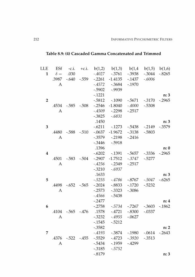
212 INFORMATIVE PSYCHOMETRIC FILTERS
Table 8.9: (4) Cascaded Gamma Concatenated and Trimmed
LLE ESf -c.i. +c.i. b(1,2) b(1,3) b(1,4 b(1,5) b(1,6)1 δ = .030 -.4027 -.3761 -.3938 -.3044 -.8265
.3987 -.640 -.559 -.2261 -1.4135 -.1437 -.6006A -.4572 -.3684 -.1970
-.5902 -.9939-.1221 n: 3
2 -.5812 -.1090 -.5671 -.3170 -.2965.4534 -.585 -.508 -.2546 -1.8040 -.4000 -.5308
A -.4509 -.2298 -.2517-.3825 -.6831.1450 n: 3
3 -.6211 -.1273 -.5438 -.2149 -.3579.4480 -.588 -.510 -.0637 -1.9672 -.3138 -.5803
A -.3579 -.2198 -.2416-.3446 -.5918.1396 n: 0
4 -.6202 -.1391 -.5657 -.3336 -.2965.4501 -.583 -.504 -.2907 -1.7512 -.3747 -.5277
A -.4256 -.2349 -.2517-.3210 -.6937.1633 n: 3
5 -.5255 -.4786 -.8767 -.5047 -.6265.4498 -.652 -.565 -.2024 -.8833 -.1720 -.5232
A -.2573 -.3323 -.3086-.4566 -.5438-.2477 n: 4
6 -.2758 -.5734 -.7267 -.3603 -.1862.4104 -.565 -.476 .1578 -.4721 -.8300 -.0337
A -.3232 -.4955 -.0627-.1545 -.5212-.3582 n: 2
7 -.4193 -.3874 -.1980 -.0614 -.2643.4376 -.522 -.455 -.5529 -.4723 -.3920 -.3513
A -.5434 -.1959 -.4299-.3185 -.5752-.8179 n: 3

NONLINEARITY, NONSTATIONARITY AND CONCATENATION 213
Table 8.10: (5) EEG control condition
LLE ESf -c.i. +c.i. b(1,2) b(1,3) b(1,4) b(1,5) b(1,6)1 δ = .030 -.4809 -.5130 -.5031 -.4853 -.7026
-.4659 -.697 -.643 -.5510 -.8330 -.6315 -.4919A -.4650 -.4649 -.6892
-.6193 -.7701-.7097 n: 4
2 -.5165 -.5564 -.4032 -.3904 -.3257-.5206 -.754 -.689 -.3961 -.5104 -.5172 -.4319
A -.5520 -.4702 -.4337 -.5084 -.3999
-.3137 n:33 -.5707 -.6562 -.6981 -.5213 -.9822
-.5778 -.764 -.698 -.4779 -1.0653 -.5449 -.5177A -.6899 -.5441 -.5724
-.7427 -.6582-.4835 n:3
4 -.5835 -.6462 -.4875 -.6077 -.8413-.3501 -.702 -.644 -.6571 -.8966 -.7204 -.6307
A -.4560 -.5690 -.6307 -.3311 -.6935
-.5230 n:45 -.5943 -.5220 -.5648 -.8248 -.4566
-.5877 -.793 -.702 -.4643 -.4269 -.6950 -.6740A -.4019 -.7060 -.5778
-.5699 -.7359-.7585 n: 1
6 -.6417 -.6922 -.6352 -.7396 -.6122-.4183 -.818 -.708 -.7996 -.6518 -.7162 -.6837
A -.4546 -.7579 -.5415 -.7587 -.5623
-.9324 n: 67 -.4430 -.3537 -.4849 -.3311 -.4242
-.4946 -.495 -.462 -.2403 -.4382 -.4840 -.4505W -.4491 -.4124 -.6066
-.3012 -.4970-.4048 n: 3

214 INFORMATIVE PSYCHOMETRIC FILTERS
Table 8.11: (6) EEG relax condition
LLE ESf -c.i. +c.i. b(1,2) b(1,3) b(1,4) b(1,5) (1,6)1 δ = .030 -.8179 -.7041 -.6143 -.5440 -.5498
-.6806 -.844 -.607 -.5612 -.8827 -.5493 -.7232W -.5275 -.6470 -.7076
-.4901 -.6115-.7683 n: 2
2 -.3435 -.3428 -.4339 -.5086 -.4778-.4543 -1.537 -.330 -.3727 -.5198 -.5154 -.4037
W -.4401 -.3836 -.3835 4163 -.5784
-.3688 n: 73 -.5784 -.6952 -.5581 -.5609 -.4763
-.6561 -.589 -.326 -.7246 -.5549 -.7149 -.8600B -.5709 -.6755 -.6035
-.7626 -.6545-.6025 n: 4
4 -.4592 -.6102 -.4473 -.4629 -.5429-.7055 -.473 -.198 -.5734 -.5066 -.6442 -.6557
B -.5957 -.4114 -.4587 -.7779 -.6349
-.6855 n: 25 -.5009 -.5867 -.5140 -.5715 -.4637
-.5820 -2.829 -1.240 -.5875 -.5798 -.3824 -.4935A -.5887 -.7528 -.5498
-.5025 -.6087-.4585 n: 2
6 -.8670 -.6597 -.7274 -1.1921 -.9999-.6152 -.824 -.261 -.7080 -.7187 -.6743 -.6710
W -.6651 -.5874 -.6209 -.6289 -.7136
-.7115 n: 57 -.2904 -.5526 -.4101 -.6620 -.4050
-.8353 -.667 -.205 -.3986 -.6061 -.5194 -.4119B -.3448 -.3510 -.5992
-.4721 -.7479-.5389 n: 1

Chapter 9
Time Series of Disasters
Disasters in British coal mines between 1851 and 1962 provide a well stud-ied data base, mainly analysed for the shape of the distribution of timesbetween successive disasters. Here the series is treated as one of variationsin the local rate of fatalities. Another series, also showing erratic fluctua-tions, sometimes due to unidentified exogenous factors, is that of the re-ported monthly sightings of UFOs in the USA over an 18-year period. Boththese series raise interesting questions for social psychologists, yet can re-quire quite different methods of analysis to explore their dynamics. Thereare big differences in temporal scale, and in the number of uncontrolledand, indeed, unidentified and uncontrollable variables, from the specifi-able psychophysics of Chapter 1, but some of the considerations aboutidentifying chaotic dynamics still surface in analogous ways.
Many real situations can generate series which are a mixture of chaotic,periodic and stochastic noise components. The actual time scale, in mil-liseconds, days, months, or years, is immaterial unless one also has moredata for interpolation. If the series are long (over 2,000 points) then itmay be possible to sample by coarsening the resolution and look for self-similarity and fractal properties, but this is not generally true. Nonstation-arity of the nonlinear dynamics, overwritten by second-order stochastic

216 INFORMATIVE PSYCHOMETRIC FILTERS
noise, is to be expected in some psychophysical and psychophysiologi-cal data. It is necessary to break a long series into successive subseries toexamine for nonstationarity, and this in itself invalidates the use of algo-rithms that depend strongly on delay coordinates in order to estimate thecorrelation dimension. It is to be expected that, even in stationary pro-cesses, the local largest Lyapunov exponent will fluctuate, approximatelyas a log normal distribution, and what is observed under nonstationarityis fluctuation from both sampling and dynamical causes. As Schaffer etal (1988) remarked, ”current methods for estimating the largest Lyapunovexponent choke on nonuniformity”, so that even if a series is long it is notnecessarily a stable basis for estimation.
The method explored here uses the fluctuations of the local largest Lya-punov exponent, the entropic analogue of the Schwarzian derivative (ESf),the confidence intervals of the ESf derived from surrogates, higher orderconvolutions in the time domain, and the eigenvalues of the matrix of theESf’s of those convolutions. It has been found that this approach can be ap-plied to series as short as 120 points; the present study now reduces thatto 72 points (each set of 72 one-month points corresponding to a six-yearperiod in the source data) to see what emerges as compared with previousanalyses in the relevant literature.
If a process is nonstationary in its parameters for all but the mostcomplicated hierarchical models, then its identification in the presenceof stochastic noise is impeded, particularly if it is simple in its stationaryepochs. However, if it is complex or chaotic, it can be more robust to theeffects of perturbing noise (Schaffer, Ellner & Kot, 1986).
The Sugihara and May (1990) approach is essentially black box, its fo-cus is on seeing if predictability is a sufficient way of distinguishing ran-dom from chaotic trajectories, under some assumptions about stationar-ity. This is still necessary, as the usual statistics, D2 and Lyapunov, arenot helpful and, indeed, dimensionality itself is not the most informativeproperty to compute for real but short biological series. As soon as a se-ries shows dead or interpolated epochs then it is not stationary, but can beput into a finite-state Markov Chain if the dead or null epochs are them-selves defined as occupying one state of the system. The problem then be-

TIME SERIES OF DISASTERS 217
comes identifying the stationarity of the state transition probability matrixin the Markov chain. Any such model needs tuning parameters (Robert &Casella, 1999); the role of the partitioning constant δ in ESf is just one suchparameter.
Limits on Identifiability
The New York measles series was used by Sugihara and May (1990) as onetest set to develop methods for discriminating between stochastic randomprocesses and chaotic processes. It is well known that such discriminationcannot always be achieved. In fact, the confusability has a practical appli-cation. Robert and Casella (1999, Chapter 2) review a number of uniformpseudo-random number generators which reproduce the behaviour of ani.i.d. sample of uniform random variables when compared through a usualset of tests. Some of these generators are mathematically chaotic attractors,which have such a long periodicity that recurrence of identical subseriesis not encountered in practical applications; that is, there are chaotic seriesthat for a specific sample of tests will pass as random. Proceeding in theopposite direction, there may be series which are essentially random bysome stochastic definition but will mimic a chaotic trajectory.
The properties of chaotic series which may be tested for as almost def-initional include sensitivity to initial conditions, local fractal dimensional-ity, positivity of the largest Lyapunov exponent, local predictability, andentropic functions. If some function of the system’s control parametersis experimentally accessible, then it may be possible to push the dynam-ics through a sequence of bifurcations, revealing Feigenbaum dynamics,which could not be done in a stochastic process. The presence of noiseand of nonstationarity or singularities will weaken the effectiveness ofsuch tests; for example, the embedding dimension of an attractor may be afixed integer, but its non-integer dimensionality on the invariant manifoldcould fluctuate. The orbits of the Lorenz equation (Davies, 1999, p.9) area well known and frequently depicted case: ”the generating point makesone or two circuits around one of the wings before switching to the other.”

218 INFORMATIVE PSYCHOMETRIC FILTERS
Each wing could be locally contained in two dimensions, but the wingsare not coplanar and it needs more dimensions to hold the whole orbits.The Shilnikov attractor is a more extreme example; it runs to the centre ofa spiral in a flat plane and then jumps out orthogonally and re-enters thespiral at its outer limit to begin the inward path again.
The frequency spectrum, and hence the autocorrelation spectrum, of achaotic process is wide with some local peaks. But a mixture of white orcoloured noise with some limited periodicity superimposed can create thesame picture. Such mixtures may have a small positive largest Lyapunovexponent. Fourier analyses may be misleading; Davies (1999, p. 56) showsthe Fourier amplitudes of the logistic map, where there is a strong period4 component, but the orbit is not periodic.
Time series which have discontinuities in them or are suspected of hav-ing some sort of instability in their generation have been the subject of adiversity of statistical methods to explore where the discontinuities arelocated, whether or not they are abrupt, and what are the best representa-tions of the discrete segments in the series lying between the discontinu-ities (Spall, 1988). In real data, there may be critical events, such as a heartattack, or a civil war, which trigger a shift in dynamics. The series may re-cover from interruptions or may be permanently changed or terminated.If the series is not isolated but has collateral variables running in their ownseries then the interaction between two or more parallel series may furnishvaluable clues about where and what disruptions have occurred.
An elegant treatment of the various commoner sorts of discontinuitiesin univariate time series was created by Gordon and Smith (in Spall, 1988,chapter 14) using state space equations. It was restricted to change pointidentification and modelling in processes in which the evolution was lin-ear between change points and the series was one of equal interval ob-servations, but is still valuable because it models, within the same equa-tions, steady-state, changes in level, change in slope, and transient outliers.However, it says nothing about higher-order dynamics, and could not beused to predict the location of the next irregularity. The series to be con-sidered here could be partly modelled by state-space equations if we wereonly interested in identifying some discontinuities as departures from a

TIME SERIES OF DISASTERS 219
hypothetical steady state. What exactly sufficiently defines a steady stateis somewhat opaque as soon as consideration of higher-order dynamicscomes into the picture.
There were many fatal accidents in the British coal mining industrybetween 1851 and 1963. The table used here from Andrews and Herzberg(1985) has a lower bound on the number of fatalities in one accident setat 10, and labels the series as one of 191 disasters. The earlier analyses byMaguire, Pearson and Wynn (1952,1953) are based on an incomplete se-ries, and treat accidents as a point process, ignoring the actual number ofdeaths involved. The focus was on comparing methods to test the non-randomness of the distribution of intervals between accidents, which ifrandom may approximate to a Poisson distribution, or to a Laplace trans-form. One might think that such an approach is unfeeling and irrespon-sible but, in fairness to those authors, they remark (p. 179): ”A thoroughstudy of time intervals between explosions in mines would take into con-sideration the number of men killed and the number at risk.” They alsocommented that, ”The problems of accidents are more human and morecomplicated than those of quality control. It is usually more importantto extract the maximum amount of information from industrial accidentdata.” Jarrett (1979) augmented the series and some internal nonunifor-mity in the rate of the process has been noted; it appears to change after125 disasters (Cox & Lewis,1966).
The series is thus long enough to be partitioned into 64, 64, and 63 suc-cessive events, to apply the same methodology as in other series. If the se-ries does, in fact, show a change in its generation process after 125 events,then the last subseries should be different from the first two. There weretechnological and social changes during this long period, but there alsoseem to have been periods of stagnation, as analysed by economists, dur-ing the late-19th century. It may be of interest that the series starts in 1851,but in 1852 the engineering employers locked out their men when they re-fused to accept systematic overtime (May, 1987, p. 236). Labour relationswere bad and labour laws were significantly loaded against workers formuch of the 19th century; legal recognition of trade unions did not occuruntil 1871. Mechanical extraction of coal from seams did not come into use

220 INFORMATIVE PSYCHOMETRIC FILTERS
in British mines until after 1900, at which date only 2 per cent of coal wasmechanically extracted.
The Deaths Series, x
The great disaster of October 1913, with over 400 deaths, stands out. Itslocation is even more marked graphically if the series variable is squared.As the series does not use accidents in which fewer than 10 persons werekilled, and we might reasonably expect that accidents involving one ortwo workers were much commoner than ones with over 10 deaths, theseries has been, in effect, low-pass filtered, so estimates of the frequencydistribution of both this series (xj) and of the time intervals series (yj)would need to be reanalysed with various cut-offs of higher values than10 if independence of successive disasters is to be examined. The totallabour force in mining, mostly coal, increased from about 200,000 in 1841to 216,000 in 1851, 496,000 in 1881, 807,000 in 1901 and to 1,128,000 in 1913(Crouzet, 1982, pp. 68, 268). After a peak of 1.2 million in 1920, the totallabour force fell steadily to 702,000 in 1938 (May, 1987, p.329). The size ofthe population at risk is therefore not constant, nor are the working condi-tions in terms of size of mine or accessibility of the coal-faces.
For this series LLE(x) = .0366
Figure 9.1: The series of 191 accidents from 1851 to 1963, x

TIME SERIES OF DISASTERS 221
Figure 9.2: The same series, squared, x2
The Time Intervals Series, y
It is this series which has been the greatest focus of statistical theorising.Tests for its randomness have taken various forms. The graphical effect ofsquaring the variable is even more marked here, emphasising the contrastin the last subseries. This is matched in the table of descriptive statistics,in the first two moments. It is not matched in the first-order ESf values,precisely because those do not use the absolute values (and hence the firsttwo moments) of the variables. Each time interval is the elapsed time indays since the previous disaster before the current one. There is, therefore,the other time series, in which the time interval is that immediately follow-ing a disaster before the next one occurs. One leads and the other lags ontime when truncated cross-correlations between the two series xj , yj andxj , y(j+1) are considered. LLE(y) = .0683
Figure 9.3: The time intervals series of 191 disasters, y
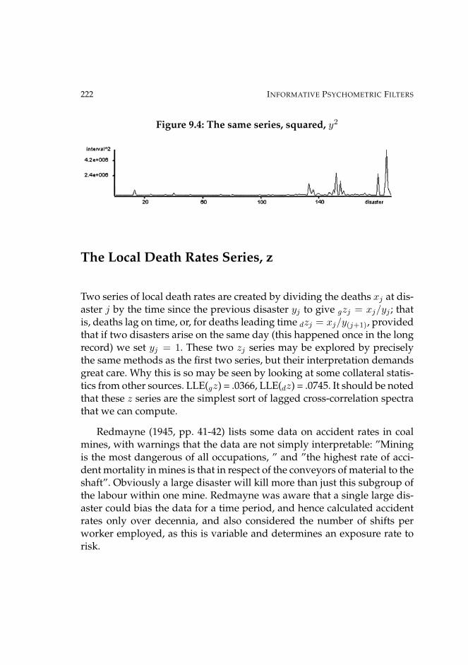
222 INFORMATIVE PSYCHOMETRIC FILTERS
Figure 9.4: The same series, squared, y2
The Local Death Rates Series, z
Two series of local death rates are created by dividing the deaths xj at dis-aster j by the time since the previous disaster yj to give gzj = xj/yj ; thatis, deaths lag on time, or, for deaths leading time dzj = xj/y(j+1), providedthat if two disasters arise on the same day (this happened once in the longrecord) we set yj = 1. These two zj series may be explored by preciselythe same methods as the first two series, but their interpretation demandsgreat care. Why this is so may be seen by looking at some collateral statis-tics from other sources. LLE(gz) = .0366, LLE(dz) = .0745. It should be notedthat these z series are the simplest sort of lagged cross-correlation spectrathat we can compute.
Redmayne (1945, pp. 41-42) lists some data on accident rates in coalmines, with warnings that the data are not simply interpretable: ”Miningis the most dangerous of all occupations, ” and ”the highest rate of acci-dent mortality in mines is that in respect of the conveyors of material to theshaft”. Obviously a large disaster will kill more than just this subgroup ofthe labour within one mine. Redmayne was aware that a single large dis-aster could bias the data for a time period, and hence calculated accidentrates only over decennia, and also considered the number of shifts perworker employed, as this is variable and determines an exposure rate torisk.

TIME SERIES OF DISASTERS 223
Figure 9.5: The gzj series;time intervals lead the number of deaths in a disaster.
Figure 9.6: The dzj seriestime intervals lag the number of deaths in a disaster.
Table 9.1Death Rate from Accidents, per 1000 employed
From Redmayne (1945), for 1873 to 1943Decade From to Rate
1 1873 1882 2.242 1883 1892 1.813 1893 1902 1.394 1903 1912 1.155 1913 1922 1.156 1923 1932 1.057 1933 1942 1.14- 1943 only 1.00

224 INFORMATIVE PSYCHOMETRIC FILTERS
Table 9.2Death rates per 100,000 man-shifts worked,
surface and underground, from 19381938 0.411939 0.371940 0.431941 0.461942 0.431943 0.36
————————————————-
It is perhaps better that we do not dwell on Redmayne’s theories (1945,p. 43) about the psychology of the miner, ”the Character and Ideocracy[sic] of the British Coal Miner”, and what he calls racial differences be-tween Celts and Danes. In interpreting the figures for 1913 to 1922, heeventually notes that the industry was under complete government con-trol during 1917 to 1921, and ”there were then strikes and unrest greaterthat at almost any other period” (no figures given). It would have beenhelpful if the relations between strike rates and death rates were tabled; itis a bit harder to get killed if one is out on strike. The whole text reads like asustained apologia for private capitalism, it was written and published ata time when nationalisation of the coal industry was under active consid-eration. Of course, that came to pass. The relevance of Redmayne’s tablesfor our current purpose is to display the changes in the generation of dataduring the total period under consideration.
When interpreting the number of deaths on one disaster, which meansfrom one mine, one needs to know how big the mine was. Crouzet (1982, p.270) notes that, ”in 1913 there were 3289 collieries worked by 1589 separatefirms. The average colliery had a workforce of 340 ... more than one thirdof the collieries were worked by fewer than 50 miners. The great majorityemployed from 50 to 2,500 without their size having any influence on theirefficiency.” If 35 miners were killed in one disaster, it means somethingquite different if the mine employed 50 men, rather than employing 500 or5,000.

TIME SERIES OF DISASTERS 225
Having got the four series x, y,g z,d z their descriptive statistics for eachsubrange may be tabulated.
————————————————-Table 9.3
Descriptive Statistics including ESf on the four seriesStatistic x1 x2 x3 y1 y2 y3
mean 41.42 53.85 58.13 113.14 133.12 395.92s.d. 55.23 55.38 83.87 137.76 115.98 464.57
variance 3050.21 3067.27 7035.17 1.8× 10⁵ 1.3× 10⁵ 2× 10⁶
Skewness 3.6026 1.9181 2.7049 2.8234 .8487 2.0776Kurtosis 15.9097 3.2257 7.5542 10.3115 -.4055 4.6043
Slope 0.1620 0.3448 -1.1566 -0.4831 1.6635 1.5907ESf -.3769 -.2322 -.1872 -.4747 -.4739 -.4301
- gz1 gz2 gz3 dz1 dz2 dz3mean 2.86 2.71 0.46 4.79 5.34 5.16
s.d. 11.53 9.44 0.75 10.38 15.98 12.63variance 132.87 89.13 0.55 107.64 255.47 159.62
Skewness 7.0063 6.1845 2.5981 3.6121 5.0138 3.7720Kurtosis 50.4346 41.7792 6.8722 14.2947 27.1255 14.9990
Slope .0407 -.0698 -.0019 -.0589 -.0993 .0979ESf -.2158 -.6152 -1.0773 -.8236 -.2161 -.2509
————————————————-
The series gzj is one in which it is assumed that an accumulator pro-cess builds up the probability of an accident over time until it is eventuallytriggered, its severity being proportional to the time for risks to accumu-late, whereas the dzj series assumes that an accident exhausts the potentialfor another accident as a function of its own severity, so that the delay tothe next accident is a proportional function of what has just occurred. Itis quite possible for the process as a whole to shift from gz to dz (or thereverse) during its evolution; this is a form of dynamical nonstationarity.
The higher-order ESf matrices can also be computed on these sub-series.

226 INFORMATIVE PSYCHOMETRIC FILTERS
Table 9.4Higher-order ESf matrices for the subseries of deaths; x
Italicised values are within the 95% c.i. for random surrogates
Block ESf b(1,2) b(1,3) b(1,4) b(1,5) b(1,6)1(of 64) -.3769 .1633 .0643 -.2771 .1338 -.0820
.4008 .1329 .2307 -.1311
.2008 .2601 .2327
.2096 -.1919-.6567 n: 5
2(of 64) -.2322 .0901 -.2261 -.2299 .3409 .1961-.0581 -.1435 -.1124 .2398-.2906 -.3552 -.0167-.1376 -.1484.2420 n: 3
3(of 63) -.1872 .3653 .2219 .2623 .2442 .1436.2610 0955 .1412 .1504.2219 .2569 .0494
-.2392 .2113.2219 n: 6
Again, the interest is in evidence of heterogeneity between the three sub-series. The ESf values for the first-order series are reduplicated for cross-checking with the previous table of descriptive statistics. From previousanalyses of time series in this fashion, it can be read that these series area mix of random and non-random higher-order relations within the se-quential dynamics, the deaths series is not one which is locally predictablewith any confidence. The deviant subseries inESf terms appears to be themiddle one, not the last one, as suggested by the earlier analyses of timeintervals by Maguire, Pearson and Wynn (1952). The middle period is theleast random in terms of higher-order dynamics, for both the deaths andthe intervals subseries. A few very disastrous accidents within a series ofmuch smaller ones can induce odd sequential dynamics.

TIME SERIES OF DISASTERS 227
Discussion
A classical problem in data analysis is that of inferring causality from acorrelation; the inference is usually invalid if unsupported by contextualknowledge. In time series, there are additional possibilities for inferringthe causal direction of links between variables. The additional informationin time series data is that which gives some insight into the temporal direc-tion of effects (as, for example, in path analysis); if the cross-correlationsin one direction at one or more lags are very different from those in theopposite direction, then some sorts of causality are supported and othersruled out. The extension from more familiar ideas here involves both thegz and dz series constructed from the two x and y data series, and theESf at first-order and higher-order values; for example, the ratios of thefirst-order ESf for gz and dz are 0.262, 2.847, and 4.294 for respectivelysubseries 1,2,3, whereas for the ratios x/y they are 0.794, 0.490 and 0.435.
It is usual to compute the cross-correlations between two parallel se-ries and see if one lags or leads upon the other. This interaction betweentwo series may itself be nonstationary and what lags at one place maylead at another. If such changes are happening, then reduction of a totalunbroken multivariate time series to one based on the Jacobians of thecross-correlations at each lag can be seriously misleading (Gregson, 1983,Chapter 6).
The four tables of higher-order ESf matrices differ from one another.Changes in one do not match changes in another but, considering the com-plicated causality of the collection of coal mines spread over regions withdifferent geology, sizes, technology, ownership, and apparently labour-management relations, there is an underlying causal heterogeneity that isnot present to anything like the same degree in the measles series. Henceany deductions are generalisations which at best will show differences be-tween different time periods.
The y series of time intervals between accidents is, indeed, nearest to aPoisson distribution if one allows the ratio of mean/s.d. to be the indicatorand the large change does then show in the last subseries where accidentsbecome rarer in time. There is not much difference in the average number

228 INFORMATIVE PSYCHOMETRIC FILTERS
of deaths (the x) series per accident over the the three subseries, but obvi-ously if one computes deaths per time (in months, and perhaps correctedfor the size of the labour force as it increased up to 1913) then conditionsimproved in one respect.
Table 9.5Higher-order ESF matrices for the subseries of intervals; y
Italicised values are within the 95% c.i. for random surrogates
Block ESf b(1,2) b(1,3) b(1,4) b(1,5 b(1,6)1(of 64) -.4747 -.0192 -.2556 -.1251 -.0468 -.2371
.0144 -.1089 -.2369 .2223-.0206 -.4565 -.0659-.0284 -.3653-.2859 n: 6
2(of 64) -.4739 -.0248 -.4247 -.4662 -.3412 .1588.1409 -.0989 -.2655 .0126
-.3062 -.1773 -.1182-.1015 -.3507.1272 n: 2
3(of 63) -.4301 .2412 .0117 -.0784 -.1403 .4620-.1386 -.0261 .0804 -.2372.2940 -.0690 -.0859
-.2283 .0285.0405 n: 3
The four higher-order ESf tables suggest that the x series is noisythroughout. The y series becomes much less noisy as it evolves, mainlydue to the fact that relatively little happens after about 1920, as technologyand prevailing economics change. This is also is reflected in the gzj series,but not in the dzj series, which is less noisy. There is thus stronger evidence

TIME SERIES OF DISASTERS 229
for an accumulator process in which the time intervals are longer after se-rious accidents. Accidents are not so much waiting to happen as manysecondary factors accumulate (as in a Poisson process) but rather that anaccident induces, for a while, more caution in all pits as knowledge of thelast disaster is diffused or knocks out, for a while, from the pool of pits atrisk those with larger current accident potential. This distinction is com-pletely lost if only the y series is analysed, as the earlier work of Maguire,Pearson and Wynn (1953) employed.
————————————————-
Table 9.6Higher-order ESf matrices for the death rates series; z
This is gzj where deaths lag on time intervalsItalicised values are within the 95% c.i. for random surrogates
Block ESf b(1,2) b(1,3) b(1,4) b(1,5) b(1,6)1(of 64) -.2158 -.1136 .0601 .1507 .1735 -.1760
-.2762 .0145 .0756 .1518.2824 .2088 .2007
-.1976 .0429.1705 n: 5
2(of 64) -.6152 -.7049 .2126 .2610 -.1863 .2610.4008 -.0978 .1134 .1102.4008 .0078 .2816
-.0434 .1344.1879 n: 5
3(of 63) -1.0773 .1610 .4008 .0247 .0651 .4008.2137 .0382 .2610 .2108.0532 .2990 .1800
-.0182 .0054.3044 n: 3
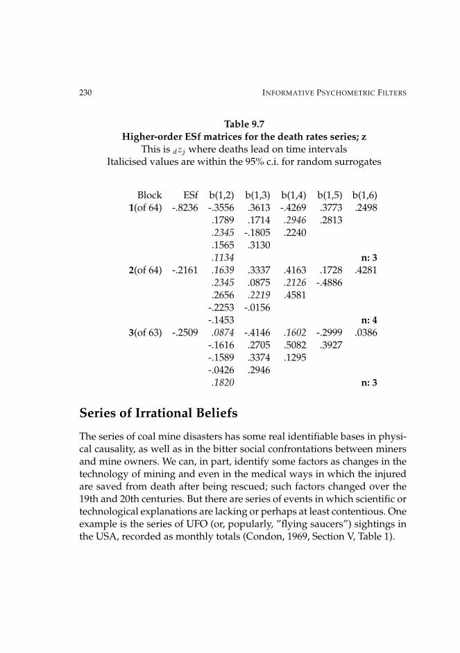
230 INFORMATIVE PSYCHOMETRIC FILTERS
Table 9.7Higher-order ESf matrices for the death rates series; z
This is dzj where deaths lead on time intervalsItalicised values are within the 95% c.i. for random surrogates
Block ESf b(1,2) b(1,3) b(1,4) b(1,5) b(1,6)1(of 64) -.8236 -.3556 .3613 -.4269 .3773 .2498
.1789 .1714 .2946 .2813
.2345 -.1805 .2240
.1565 .3130
.1134 n: 32(of 64) -.2161 .1639 .3337 .4163 .1728 .4281
.2345 .0875 .2126 -.4886
.2656 .2219 .4581-.2253 -.0156-.1453 n: 4
3(of 63) -.2509 .0874 -.4146 .1602 -.2999 .0386-.1616 .2705 .5082 .3927-.1589 .3374 .1295-.0426 .2946.1820 n: 3
Series of Irrational Beliefs
The series of coal mine disasters has some real identifiable bases in physi-cal causality, as well as in the bitter social confrontations between minersand mine owners. We can, in part, identify some factors as changes in thetechnology of mining and even in the medical ways in which the injuredare saved from death after being rescued; such factors changed over the19th and 20th centuries. But there are series of events in which scientific ortechnological explanations are lacking or perhaps at least contentious. Oneexample is the series of UFO (or, popularly, ”flying saucers”) sightings inthe USA, recorded as monthly totals (Condon, 1969, Section V, Table 1).
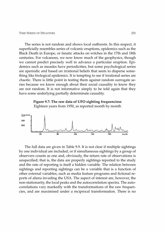
TIME SERIES OF DISASTERS 231
The series is not random and shows local outbursts. In this respect, itsuperficially resembles series of volcanic eruptions, epidemics such as theBlack Death in Europe, or fanatic attacks on witches in the 17th and 18thcenturies. For volcanoes, we now know much of the geophysics, thoughwe cannot predict precisely well in advance a particular eruption. Epi-demics such as measles have periodicities, but some psychological seriesare aperiodic and based on irrational beliefs that seem to disperse some-thing like biological epidemics. It is tempting to see if irrational series arechaotic. There is little point in testing them against random surrogate se-ries because we know enough about their social causality to know theyare not random. It is not informative simply to be told again that theyhave some underlying partially determinate causality.
Figure 9.7: The raw data of UFO sighting frequenciessEighteen years from 1950, as reported month by month
The full data are given in Table 9.9. It is not clear if multiple sightingsby one individual are included, or if simultaneous sightings by a group ofobservers counts as one and, obviously, the return rate of observations isunspecified; that is, the data are properly sightings reported to the studyand the rate of reporting is itself a hidden variable. The relation betweensightings and reporting sightings can be a variable that is a function ofother external variables, such as media feature programs and fictional re-ports of aliens invading the USA. The aspect of interest are, however, thenon-stationarity, the local peaks and the autocorrelation spectra. The auto-correlations vary markedly with the transformations of the raw frequen-cies, and are maximised under a reciprocal transformation. There is no

232 INFORMATIVE PSYCHOMETRIC FILTERS
suggestion of an annual periodicity. Showing where and how the non-stationarity arises demands that the series is explored under other trans-formations and using filters in the sense of Chapter 1; a low pass filtermerely repeats the pattern of Figure 9.7 with smoothing the peaks, a high-pass filter is now much more informative. This is shown in Figures 9.8and 9.9. Calculating indices of chaoticity on filtered series is not commonlydone, but we note that Abarbanel (1996, page 93) anticipates this when hewrites, ”we are seeing data with small scale motions suppressed yet withvery interesting dynamics How the Lyapunov exponents of a system varywith spatial averaging is the issue.”
If we wish to use symbolic dynamics (Gregson, 2005), then the UFOsightings series has to be coarse scaled by partitioning into a closed setof segments and labelling the segments each with a dummy variable. Wewill use 5 segments and then put the data into a 5-state Markov transitionprobability matrix. The simplest partitioning is into equal width ranges, amaximum a priori entropy assumption. This is in fact false, the low valuesas much commoner, so three solutions are presented.
Figure 9.8: Reciprocals of monthly UFO sighting frequenciesderived From Figure 9.7
Table 9.12 ( see also Figure 9.7) is based on using the reciprocals of theraw frequencies, which thus expresses the process in terms of local ratesof sightings. This also gives us a long term prediction of the frequencyand rate distributions, coarse scaled, of UFO sightings after 1968, underassumptions of stationarity dynamics.
The series is long enough to get some estimates of the largest Lya-

TIME SERIES OF DISASTERS 233
Figure 9.9: Highpass filtering of UFO sighting frequenciesderived From Figure 9.7
punov exponent (LLE). In all cases it is positive but very small, suggestingedge-of-chaos; For raw frequency data, LLE = +.0394, for a log10 trans-form, +.0862, for reciprocals, +.0335, for high pass filtering, +.0478, and forlow pass filtering +.0643.
ESf are computable, for the full series ESf =-.5745 with δ = .005, for thefirst 9 years,-.5009, and for the last 9 years -.4810. This is compatible withthe appearance of non-stationarity.
————————————————-Table 9.8 Autocorrelation Spectra under Transformations
The raw frequencies, their logs and their reciprocals are tabled in parallel.
lag autocorrel log10 trans reciprocal1 .5938 .7418 .76112 .2640 .5392 .53573 .1481 .4220 .41194 .0672 .3177 .35015 .0222 .2305 .31566 .0197 .1915 .31037 .0585 .1751 .29228 .0436 .1922 .27689 .0014 .1718 .2543
10 -.0139 .1737 .2662

234 INFORMATIVE PSYCHOMETRIC FILTERS
So the partitioning points are 0,.2,.4,.6,.8,1.0 for Table 9.8, and (quitearbitrarily and heuristically) 0,.1,.2,.6,.9,1.0 for Table 9.9. The reciprocalshave a skewed distribution so 0,.02,.04,.08,.2,1.0 have been used.
The stationary state vectors in Tables 9.10, 9.11, and 9.12 are based onobserved convergence after 20 iterations. The most interesting and poten-tially informative are those from the reciprocals of the frequencies in Table9.12.
Table 9.9: Monthly Returns on UFO sightings
Jan Feb Mar Apr May Jun Jul Aug Sep Oct Nov Dec1950 15 13 41 17 8 9 21 21 19 17 14 151951 25 18 13 6 5 6 10 18 16 24 16 121952 15 17 23 82 79 148 536 326 124 61 50 421953 67 91 70 24 25 32 41 35 22 37 35 291954 36 20 34 34 34 51 60 43 48 51 46 301955 30 34 41 33 54 48 63 68 57 55 32 251956 43 46 44 39 46 43 72 123 71 53 56 341957 27 29 39 39 39 35 70 70 59 103 361 1361958 61 41 47 57 40 36 63 84 65 53 33 371959 34 33 34 26 29 34 40 37 40 47 26 101960 23 23 25 39 40 44 59 60 106 54 33 511961 47 61 49 31 60 45 71 63 62 41 40 211962 26 24 21 48 44 36 65 52 57 44 34 231963 17 17 30 26 23 64 43 52 43 39 22 221964 19 26 20 43 83 42 110 85 41 26 51 151965 45 35 43 36 41 33 135 262 104 70 55 281966 38 18 158 143 99 92 93 104 67 126 82 401967 81 115 165 112 63 77 75 44 69 58 54 24
Mitchener and Nowak (2004) found a transition matrix for a pro-cess which they considered resembling a Shilnikov attractor trajectory; inthis 5-state representation, the upper left 3 × 3 submatrix is one part ofthe system, which is fully connected, the lower right 2 × 2 high ampli-

TIME SERIES OF DISASTERS 235
tude part represents a subregion into which the trajectory can transientlyjump. These dynamics are chaotic but, in a short realisation, appear non-stationary. We return to this topic in the next chapter. Another way of vi-sualising the system is to think of the 3 × 3 submatrix as partitioning thesystem’s dynamics and the transient jumps to constitute themselves a slowseries with aperiodic intervals between the jumps.
Table 9.10: 5-state transition matrix with equal partitioningThe last columns are the respective stationary state vectors
.967 .029 .005 .000 .000 .9330
.545 .273 .000 .182 .000 .0491
.000 1.000 .000 .000 .00 .0045
.500 .000 .000 .000 .500 .0089
.000 1.000 .000 .000 .000 .0045
Table 9.11: 5-state transition matrix with skewed partitioning
.884 .116 .000 .000 .000 .7319
.378 .467 .156 .000 .000 .2010
.167 .333 .333 .167 .000 .0537
.000 .500 .000 .000 .500 .0090
.000 .000 1.000 .000 .000 .0045
Table 9.12: 5-state transition matrix for reciprocal values
.671 .278 .051 .000 .000 .3491
.247 .613 .140 .000 .000 .4080
.070 .256 .558 .116 .000 .2009
.000 .250 .375 .250 .125 .0374
.000 .000 .000 1.000 .000 .0047

236 INFORMATIVE PSYCHOMETRIC FILTERS
In Table 9.12, the meaning of fast and slow submatrices is reversed: the up-per 3× 3 submatrix is now associated with slow dynamics, and the lowerright 2 × 2 submatrix with faster changes. Because of the social changesin UFO beliefs it is very doubtful if the stationary state vectors have anylong-term validity; possibly they could be replaced by beliefs in terrorism,as another form of social near-panic. Even more transitory were the mil-lennial vigils around the year 2000 (Gregson and Gregson,1999).
An argument might be advanced for treating series such as the UFOsightings as convolutions of a least two other processes: a social inertia orcontaminative effects within a social group, and perturbations from criticalincidents in the cultural environment. That would lead us back into par-allels with the spread of infectious diseases about which many stochasticmodels have been developed; some examples were noted in the last partof Chapter 1.
Note
The coal mine disasters series are taken from Andrews and Herzberg(1985).
The UFO sighting frequencies are taken from a US Air Force commis-sioned report by Condon (1969).

Chapter 10
Perron-Frobenius at the Edgeof Chaos
From the approach of symbolic dynamics, any psychophysiological timeseries may be given a square non-negative matrix representation that isthen treated as the generator of a Markov chain. This has eigenvalues that,if the matrix is scrambled, that is effectively not degenerate, give a pictureof the complexity of the dynamics. That picture is computed for two timeseries: one theoretical and homogeneous, resembling a Shilnikov attractor,and the other from real physiological data that are very unstable with tran-sient outliers. A comparison is made with indices of entropy and chaos foreach of 10 data sub-blocks. No index in itself provides a satisfactory repre-sentation of the total dynamics, but the differences between the indices areintrinsically informative. Assumptions of linearity are universally invali-dated. The use of the entropic analogue of the Schwarzian derivative (ESf)leads naturally into the calculation of Kullback-Leibler information mea-sures as asymmetric proximity indices between subseries of the data. Thefull matrix of these indices has eigenvalues that are informative concern-ing the non-stationarity of the process. The matrices that we create for arepresentation of psychophysiological and psychophysical time series areMarkovian, and are necessarily square and non-negative. They may also

238 INFORMATIVE PSYCHOMETRIC FILTERS
be sparsely filled, and quasi-cyclic. We know both from the fundamen-tal mathematics, and from examples constructed (Mitchener and Nowak,2004) that, if we accept the positivity of the largest Lyapunov exponents asa sufficient indication of chaos, of one sort, then the processes being repre-sented in transition probability matrix form may be chaotic. Possibly themost important extension of these ideas is to non-homogeneous Markovchains as a structure for non-stationary psychophysics.
As I will want to examine some real and theoretical Markovian ma-trices and their associated eigenvalues, it is proper to begin by restatingthe Perron-Frobenius theorem (Frobenius, 1912, Seneta, 1973) for primi-tive matrices: Suppose that T is an n × n non-negative primitive matrix.Then there exists an eigenvalue r such that:
(a) r real, > 0;
(b) with r can be associated strictly positive left and righteigenvectors;
(c) r > |λ| for any eigenvalue λ 6= r;
(d) the eigenvalues associated with e are unique to constantmultiples;
(e) if 0 ≤ B ≤ T and β is an eigenvalue of B, then |β| ≤ r,and |β| = r impies B = T .
(f) r r is a root of the characteristic equation of T .
There are other statements that hold from this theorem (Ding and Fay,2005) which find application in the estimation of geometrical limits in n-space.
I am also going to need to make reference to the well-known scram-bling property of Markov matrices, namelyAn n× n stochastic matrix p+ pij is called a scrambling matrix, if givenany two rows α and β there is at least one column, γ, such that pαγ > 0and pβγ > 0.
A corollary follows: if Q = qij is another stochastic matrix, then forany Q, QP is scrambling, for fixed scrambling P .
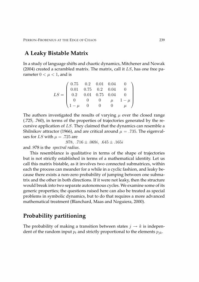
PERRON-FROBENIUS AT THE EDGE OF CHAOS 239
A Leaky Bistable Matrix
In a study of language shifts and chaotic dynamics, Mitchener and Nowak(2004) created a scrambled matrix. The matrix, call it LS, has one free pa-rameter 0 < µ < 1, and is
LS =
0.75 0.2 0.01 0.04 00.01 0.75 0.2 0.04 00.2 0.01 0.75 0.04 00 0 0 µ 1− µ
1− µ 0 0 0 µ
The authors investigated the results of varying µ over the closed range(.725, .760), in terms of the properties of trajectories generated by the re-cursive application of LS. They claimed that the dynamics can resemble aShilnikov attractor (1966), and are critical around µ = .735. The eigenval-ues for LS with µ = .725 are
.978, .716± .069i, .645± .165iand .978 is the spectral radius.
This resemblance is qualitative in terms of the shape of trajectoriesbut is not strictly established in terms of a mathematical identity. Let uscall this matrix bistable, as it involves two connected submatrices, withineach the process can meander for a while in a cyclic fashion, and leaky be-cause there exists a non-zero probability of jumping between one subma-trix and the other in both directions. If it were not leaky, then the structurewould break into two separate autonomous cycles. We examine some of itsgeneric properties; the questions raised here can also be treated as specialproblems in symbolic dynamics, but to do that requires a more advancedmathematical treatment (Blanchard, Maas and Noguiera, 2000).
Probability partitioning
The probability of making a transition between states j → k is indepen-dent of the random input pt and strictly proportional to the elements pjk.

240 INFORMATIVE PSYCHOMETRIC FILTERS
The row sums of pjk in LS are all unity, by definition. So take the unitinterval (> 0, 1) within which the random variable pt lies, and partition itin line segments s1, s3, s3 proportionately to the defined values of pjk inS1, S2, S3, and similarly for µ, 1 − µ in S4, S5. Then if and only if pt lies insegment sjk, given Sj , the resulting transition is j → k. This conventionpreserves the Markov structure of LS.
An estimate of the stationary state vector from a generated sample se-ries is
.078, .402, .273, .134, .111
Table 10.1: Descriptive statistics of a sample LS seriesBlock LLE mean Kurt ESf D2 H ApEn1-180 +.051 2.79 -0.353 -1.2541 1.716 .2837 0.535
Key: Block: iterations. LLE: largest Lyapunov exponent. mean: averagecoded state. Kurt: kurtosis. ESf: entropic analogue of Schwarzian deriva-tive (Gregson, 2002). D2: fractal dimensionality. H: Hurst index. ApEn: ap-proximate entropy (k = 10, δ = .005).
A Tremor Series
A series with a very unstable appearance and irregular transient extremedeviations is s14r45of.d from the PhysioNet archives. Only the first 4000steps are used, in 10 blocks of 400. The dynamics are, on visual inspection,nonlinear and non-stationary. Deviations can be isolated in time or come inbursts. Every estimate of the largest Lyapunov exponent has been positivebut, in some cases, marginal.
These series are wildly fluctuating and their irregularity is reflected inmost of the computed indices. It is recognised that complexity changesin time series as detected by information (entropy) measures (Tores andGamereo, 2000). The distribution of the dependent variable (as in the ver-tical axes in the graphs) is nothing like Gaussian, and would not he read-ily represented in the frequency domain, as Fourier analyses cannot han-

PERRON-FROBENIUS AT THE EDGE OF CHAOS 241
Figures 10.1, 10.2, 10.3: Blocks of the Tremor Series
dle local aperiodic spikes. Autocorrelations would be similarly misleadingexcept as long-term averages. It is possible to treat this sort of series in aMarkov chain filtering. It is possible that the leaky bistable matrices in-troduced by Mitchener and Nowak (2004) are a candidate model. Thereappear to be two levels of tremors, low amplitude high frequency and in-termittent aperiodic high amplitude, which co-exist. High-pass and low-pass filtering could be used to partial these out.

242 INFORMATIVE PSYCHOMETRIC FILTERS
Table 10.2: Descriptive statistics of Parkinsonian Tremor series
Block LLE mean Kurt ESf D2 H ApEn1-400 +.034 .812 133.41 -.3897 1.835 .1647 1.112
401-800 +.078 .717 19.63 -.5572 1.806 .1928 1.122801-1200 +.083 .529 6.43 -.5027 1.806 .1937 1.120
1201-1600 +.052 .725 71.66 -.5578 1.780 .2200 1.1881601-2000 +.009 1.033 156.22 -.5025 1.932 .0684 1.0922001-2400 +.073 .831 5.93 -.6258 1.788 .2118 1.2452401-2800 +.096 .640 5.82 -.6642 1.790 .2103 1.2502801-3200 +.065 .937 23.80 -.6354 1.780 .2201 1.2593201-3600 +.080 .756 5.17 -.6146 1.836 .1641 1.2193601-4000 +.023 1.106 122.78 -.4891 1.750 .2498 1.111
– – – – – – – –cftv .449 .207 1.045 .145 .298 .250 .054regr 1 -4.94 -1874.52 -1.89 -5.08 0.78 1.44corr 1 .825 .910 .660 .289 .461 .635
Key: Block: beats in sequence. LLE: largest Lyapunov exponent. mean:average i.b.i. Kurt: kurtosis. ESf: entropic analogue of Schwarzianderivative (Gregson, 2002). D2: fractal dimensionality. H: Hurst in-dex. ApEn: approximate entropy (k = 10, δ = .005). cftv: co-efficient of variation (σ/|µ|). regr: slope of regression of variableon LLE. corr: product-moment correlation of LLE with variable.
————————————————-The ESf and LLE measures can have associated confidence limits or fil-tered estimates computed as well, giving more insight into the variabilitybetween successive blocks of data. Comparing Tables 10.2 and 10.3 we seeimmediately that all the ESf values are outside their random surrogate 95%c.i. range; none of the blocks are random i.i.d. series.
The reason for computing the LLE values after low or high pass filter-ing is to explore the possibility that the chaotic component is either in aslow carrier wave or a fast low-amplitude part; this will only work if the

PERRON-FROBENIUS AT THE EDGE OF CHAOS 243
fast and slow parts are widely separated in their dynamics. In this series,both the slow and the fast components are associated with the transientaperiodic outlier spikes, suggesting that there are three dynamical sub-systems involved. There are still computational difficulties, as LLE valuesfrom short time series are liable to be biased (Rosenstein, Collins and DeLuca, 1993), the blocks here are much shorter than what physicists like tocall short.
————————————————-Table 10.3: Further c.i. statistics of Table 10.2
Block LpLLE HpLLE -rsESf rsESf +rsESf1-400 +.069 +.055 -.167 -.146 -.125
401-800 +.077 +.103 -.280 -.269 -.258801-1200 +.114 +.113 -.363 -.349 -.336
1201-1600 +.093 +.029 -.242 -.223 -.2041601-2000 +.036 +.034 -.224 -.208 -.1922001-2400 +.090 +.101 -.338 -.327 -.3152401-2800 +.127 +.125 -.397 -.389 -.3812801-3200 +.069 +.086 -.314 -.302 -.2903201-3600 +.118 +.093 -.375 -.363 -.3513601-4000 +.059 +.031 -.161 -.143 -.125
Key: LpLLE: LLE after low pass filter. HpLLE: LLE after high pass filter. -rsESf: lower 95% c.i. bound for random surrogate ESf. rsESf: mean randomsurrogate ESf. +rsESf: upper 95% c.i. bound for random surrogate ESf.
————————————————-
In Table 10.4 the spherical radius is the same as the largest eigenvalue,Egv 1. Note that the number of complex conjugate pairs in the roots isnot necessarily the same as for the LS matrix, which has quite differentand homogeneous dynamics. These real data are not stationary and henceare treated in short blocks to expose the breakdown of homogeneity. Notethat the dynamics drift over the total series of 4,000 data points; in some

244 INFORMATIVE PSYCHOMETRIC FILTERS
epochs the outlying tremors seem to be predominantly in one direction,in others in the opposite one. In blocks 5 and 6 the effective rank of thematrix reduces to 4.
Table 10.4: Eigenvalues of Markov matrices of the Tremor Series
Block Egv 1 Egv 2 Egv 3 Egv 4 Egv 51 1.000 .291 -.2 .041 + .066i .041 - .066i2 1.001 .316+.015i .316-.015i .021 .0123 1.000 .283 -.063 .052+.024i .052-.024i4 .999 .381 .236 .103 -.0055 .999 .259 -.056 -.002 < .0016 1.044 .237 -.048 .028 < .0017 .999 .314 .118 -.064 -.0028 .999 .219+.046i .219-.046i .165 -.0069 .999 .351 .234 .115 .068
10 1.004 .496 -.010 + .051i -.010 - .051i -.006
The values of Egv 1> 1 are computational errors, the largest eigenvalue ofa row stochastic matrix is less than or equal to unity (Karpelevich, 1951).The stationary state vectors are the solution of the matrix equation
T∞ = M∞T0
The state S5 refers to the largest positive transient tremors, expressed asdeviations from a resting position. The solutions in Tables 10.4 and 10.5have to be obtained by shifting, in some blocks, the partitions that createthe state occupancies from the raw data sequences, as the tremors are veryirregular in direction and amplitude as well as their inter-tremor intervals.In all cases, I have moved partitions, where necessary, to span the rescaledvalues and to ensure that all states are occupied. The transition probabilitymatrices are then in all cases scrambled.

PERRON-FROBENIUS AT THE EDGE OF CHAOS 245
Information measures as non-stationarity indices
The Schwarzian derivative has a long history but its importance in nonlin-ear dynamics only emerged relatively recently (Gregson, 1988). Combin-ing this derivative of C3 diffeomorphisms with an entropy measure overlocal short time-series is an exploratory innovation which has some usefulproperties. We repeat some of the definitions here as a precursor to usingthe measure in Kullback-Leibler form.
————————————————-Table 10.5: Stationary state vectors for Table 10.4.
Block p(S1) p(S2) p(S3) p(S4) p(S5)1 .0485 .0485 .3495 .5340 .01942 .0977 .2882 .4662 .1429 .00503 .0676 .0675 .3076 .5323 .02514 .0201 .1378 .7569 .0827 .00255 .0301 .8346 .1228 .0100 .00256 .0102 .0050 .0077 .0402 .93697 .0226 .0125 .0276 .3985 .53888 .0376 .1028 .7268 .1303 .00259 .0526 .0852 .1679 .6792 .0150
10 .0178 .7053 .2694 .0051 .0025
————————————————-
Schwarz (1868) defined the derivative
Sf :=f
′′′
f ′ −32
(f
′′
f ′
)2
[10.1]
which is of interest in dynamics because its value indicates the extentto which a process expands to fill a local region of the phase space.
Using successive differencing of a time-series, the total information Iin the distribution of the mth differences over k exhaustive mutually ex-

246 INFORMATIVE PSYCHOMETRIC FILTERS
clusive partitions is
I(m) := −K∑h=1
phlogs(ph)|m [10.2]
Using [10.2], suppose that we substitute within [10,1] I(m) values for fm,so that, for example, I(3) corresponds to f
′′′, employing I(m) summed over
the whole range of k subranges in each case. This is to create an entropicanalog of the Schwarzian derivative. Then, by definition, ESf (Gregson,2002) has the form
ESf :=I(3)
I(1)− 3
2
(I(2)
I(1)
)2
[10.3]
Note that [10.3] is defined at least over triplets within a series; the way inwhich the I(m) is computed drops the actual real measurement units of thedata and deliberately loses the first and second moments of the series.
If the data in one subseries are taken as generated by a basic symbolicprocess X unperturbed by transients, then the probability distribution ofthe absolute differences of orders one, two, three in that block that are com-puted for ESf estimation can be used as estimates of pi(X|θ), i = 1, .., 10in the Kullback-Leibler expression
I(Y,X) =5∑i=1
pi(Y ) · log(pi(Y )Xi|θ
)[10.4]
and that may be taken as a relative mismatch distance, not a true metricdistance, because of asymmetry, but a dissimilarity.
Every one of the 10 blocks can in turn be used as the predictor X forthe set of 10 Y . The dissimilarity of a set with itself is zero, and the fullmatrix of the differences are set out in Tables 10.6,10.7, and 10.8. Each rowis for a fixed predictorX against which all the 10 Y are compared, runningdown from X1 to X10.
These matrices indicate where the variability in information content ofthe blocks differs without having to commit to a single generating modelas theory. Using each block in turn as predictor under some assumptions

PERRON-FROBENIUS AT THE EDGE OF CHAOS 247
about error-minimal distributions is an approach reminiscent of EmpiricalBayesian statistics. The eigenvalues of these K-L matrices can, in turn, becomputed, giving some insight into the role of successive differences inthe system’s dynamics. If the matrices for differences of different orders1,2,3 show similar patterns of values, this suggests that the underlyingtime series are self-similar, which is a property of fractal dynamics.
To compare these three matrices in Tables 10.6, 10.7, 10.8, we may pro-ceed in two ways: just compute the cell-by-cell correlations to see if thematrices treated as 100-term vectors are similar, or find the eigenvectors ofeach matrix.
————————————————-Table 10.6: Based on absolute first differences, k = 10.
A Kullback-Leibler matrix of asymmetrical dissimilarities
1 2 3 4 5 6 7 8 9 10.000 3.242 5.093 .209 .134 5.093 6.567 4.838 6.499 .113.725 .000 5.217 .557 .650 5.228 4.039 7.774 3.995 .876
1.183 2.631 .000 .915 1.300 .004 5.227 3.215 5.377 1.714.184 3.719 5.292 .000 .052 5.296 7.024 4.931 7.003 .333.172 3.603 6.757 .079 .000 6.757 7.421 6.182 7.342 .202
1.185 2.676 .004 .925 1.299 .000 5.395 3.341 5.541 1.7281.658 .648 4.055 1.309 1.687 4.078 .000 4.188 .055 1.8091.244 6.632 3.605 .819 1.122 3.617 6.220 .000 6.350 1.5061.562 .586 5.754 1.280 1.528 5.772 .058 5.861 .000 1.533.124 2.891 6.308 .365 .180 6.309 5.436 5.852 5.289 .000
The eigenvalues of the first differences matrix Table 10.6 are
26.0407, -12.0417, -6.5640 + .3251i, -6.5640 - .3251i -.5446-.2028, -.1004, -.0136, -.0083, -.0012
in descending order and the last four may be neglected. Note the complexconjugate pair that arises when the matrix is not skew symmetrical aboutthe leading diagonal of zeroes.
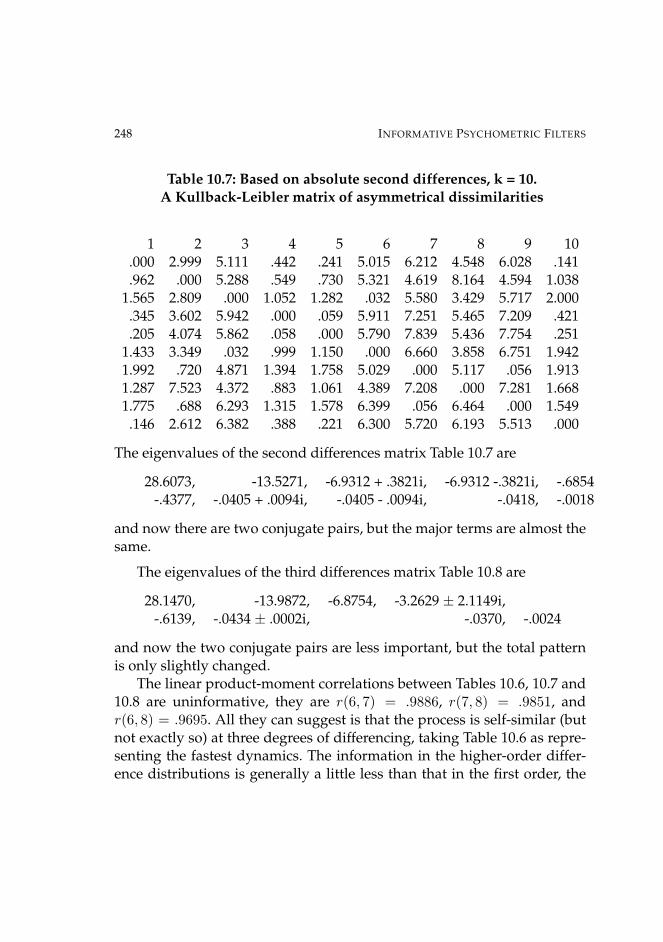
248 INFORMATIVE PSYCHOMETRIC FILTERS
Table 10.7: Based on absolute second differences, k = 10.A Kullback-Leibler matrix of asymmetrical dissimilarities
1 2 3 4 5 6 7 8 9 10.000 2.999 5.111 .442 .241 5.015 6.212 4.548 6.028 .141.962 .000 5.288 .549 .730 5.321 4.619 8.164 4.594 1.038
1.565 2.809 .000 1.052 1.282 .032 5.580 3.429 5.717 2.000.345 3.602 5.942 .000 .059 5.911 7.251 5.465 7.209 .421.205 4.074 5.862 .058 .000 5.790 7.839 5.436 7.754 .251
1.433 3.349 .032 .999 1.150 .000 6.660 3.858 6.751 1.9421.992 .720 4.871 1.394 1.758 5.029 .000 5.117 .056 1.9131.287 7.523 4.372 .883 1.061 4.389 7.208 .000 7.281 1.6681.775 .688 6.293 1.315 1.578 6.399 .056 6.464 .000 1.549.146 2.612 6.382 .388 .221 6.300 5.720 6.193 5.513 .000
The eigenvalues of the second differences matrix Table 10.7 are
28.6073, -13.5271, -6.9312 + .3821i, -6.9312 -.3821i, -.6854-.4377, -.0405 + .0094i, -.0405 - .0094i, -.0418, -.0018
and now there are two conjugate pairs, but the major terms are almost thesame.
The eigenvalues of the third differences matrix Table 10.8 are
28.1470, -13.9872, -6.8754, -3.2629 ± 2.1149i,-.6139, -.0434 ± .0002i, -.0370, -.0024
and now the two conjugate pairs are less important, but the total patternis only slightly changed.
The linear product-moment correlations between Tables 10.6, 10.7 and10.8 are uninformative, they are r(6, 7) = .9886, r(7, 8) = .9851, andr(6, 8) = .9695. All they can suggest is that the process is self-similar (butnot exactly so) at three degrees of differencing, taking Table 10.6 as repre-senting the fastest dynamics. The information in the higher-order differ-ence distributions is generally a little less than that in the first order, the

PERRON-FROBENIUS AT THE EDGE OF CHAOS 249
Table 10.8: Based on absolute third differences, k = 10.A Kullback-Leibler matrix of asymmetrical dissimilarities
1 2 3 4 5 6 7 8 9 10.000 2.844 4.562 .295 .359 4.365 5.596 4.178 5.215 .078.951 .000 5.732 .551 .611 5.823 5.514 8.297 5.506 .963
1.527 3.067 .000 1.155 1.371 .088 6.123 3.650 6.196 1.868.245 3.250 5.891 .000 .042 5.826 7.011 5.557 6.894 .305.293 3.078 6.879 .043 .000 6.809 8.046 6.578 7.941 .337
1.318 3.941 .082 1.065 1.254 .000 7.861 4.384 7.819 1.7221.885 .872 5.629 1.443 1.654 5.923 .000 5.815 .079 1.8541.244 7.616 4.052 .963 1.165 4.104 7.352 .000 7.350 1.5931.475 .860 6.169 1.241 1.441 6.328 .087 6.269 .000 1.405.068 2.290 5.464 .313 .364 5.286 5.361 5.199 4.980 .000
————————————————-
distributions are more skewed towards the lower end. As noted above, thescalar values of the differences, that is their first and second moments, areremoved in this analysis, the entropies are scale-independent.
Discussion
As the tremor series can be partitioned approximately into fast and slowdynamics, it is proper to ask where the non-stationarity arises? Taking theevidence of all the relevant tables together, it is seen that the faster dynam-ics are relatively stable in their evolution, but the slower dynamics fluctu-ate from block to block. If one thinks of the slower dynamics as a carrierwave, a stable base for supporting faster dynamics sensitive to exogenouseffects or to internal nonlinearities, that is in this case wrong.
The analysis in Tables 10.6, 10.7 and 10.8 pools over all the 10 blocks, soit is orthogonal to the previous analyses in Tables 10.2, 10.3, 10.4 and 10.5

250 INFORMATIVE PSYCHOMETRIC FILTERS
done block by block. Only the ESf estimates in these four blockwise tablesis a hidden bridge between the two orthogonal analyses.
Dynamics of Cardiac Psychophysiology
Some patients undergoing bio-feedback therapy for respiratory disordersdo have panic episodes, as they themselves relate. Others do not. Thecausality and even the detailed dynamics of panic episodes are the sub-ject of considerable controversy (Baker, 1992) and these wider questionsare not being entered into here. Rather, our starting point is the fact thatpalpitations and a local rapid raise in heart rate are the most frequentlyobserved characteristic properties of a panic attack, irrespective of the en-vironmental or intrasubjective situations that appear to trigger the onset.The measures of heart rate activity cited in the relevant literature are usu-ally the rate, in beats/minute, and nothing else. More complex analyses ofthe sequential dynamics of the heart activity are not usual, partly becausethe resources available to researchers, both in terms of recording apparatusand mathematical software for subsequent analysis, are relatively recent intheir development. The idea that we should investigate the nonlinear dy-namics of the heart under conditions when there is no panic, as a possiblepredictor of panic susceptibility, is virtually untested. At the same time, itis known that cardiac dynamics are intrinsically difficult to model, partlydue to their lability and complexity, and contradictory explanations havebeen advanced for rhythm generation (Dunin-Barkowski, Escobar, Lover-ing & Orem, 2003).
Gorman and Sloan (2000) review a number of studies in which it isshown that, under non-panic conditions, patients with panic disorders ap-pear to have diminished heart rate variability. In turn, diminished vari-ability is a precursor of myocardial infarction, in short, a good predictorof death, and self-report of panic attacks and higher anxiety can be associ-ated both with lower levels of heart rate variability and increased risk offatal coronary heart disease (Kawachi, Sparrow & Vokonas, 1994).
This investigation is in two parts: an examination of data from one

PERRON-FROBENIUS AT THE EDGE OF CHAOS 251
subject to establish the viability of some of the methodology, and a partin which comparison of some heart beat time series of clinical interest aremade using the methods established in the first part.
The first part consists of three epochs, in sequence, each about 5 min-utes long. All the three epochs were truncated at 386 interbeat intervals,which time evolution spans approximately five minutes of continuousrecording. As the third epoch was deliberately made to be non-stationary,with a brief burst of shallow rapid breathing, the treatment of that se-ries as internally homogeneous is strictly wrong, but is first presentedthat way, as in the same way as the first two epochs, as an example ofthe type of error that ignoring nonstationarity or nonlinearity can create(Bunde, Kropp & Schellnhuber, 2002). It is now expected that nonstation-arity, better described as the consequences of chaotic itinerancy (Kaneko& Tsuda, 2003), is characteristic of heart activity, where normal dynamicregulation involves return to some attractor basin or basins after transientdestabilization (Gorman & Sloan,2000). As has been known for some time,analyses that use linear statistical modelling, either static or with time se-ries assumptions, can obscure the very properties of the dynamics that areboth clinically interesting and indeed necessary for the individual’s long-term survival (Barndorff-Nielsen, Jensen and Kendall, 1993; Medvinsky,Rusakov, Moskalenko, Fedorov, & Panfilov, 2003).
We note that many of the methods for examining nonlinear time seriesand their associated dynamics were anticipated in mathematical psychol-ogy as long ago as 1960, by Licklider. The main additions now to whatwas available then centre on chaotic dynamics, the underlying entropyand time series concepts have their origins in the late 19th century. Theconventional distributional statistics are as follows, intercept and slope re-fer to a linear regression over time, the variable in most cases is pulse ratein beats/min. The time series are made up of about 900 interbeat intervals,and normally each of these is about 700-800 millisecs; each starts with thedepolarisation peak of the cycle. The nonlinear statistics in Table 10.9 areagain LLE, ESf, and ApEn. Low pass and high pass refer to the series afterfiltering:

252 INFORMATIVE PSYCHOMETRIC FILTERS
————————————————-Table 10.9: descriptive statistics
measures Epoch001 Epoch002 Epoch003min 687 640 300max 843 847 1011
mean 761.13 770.55 758.60s.d. 33.69 33.82 117.92
Skewness .003 -.983 -2.143Kurtosis -.643 1.632 5.151intercept 772 751 708
slope -.057 +.101 +.221LLE .091 .103 .090
Low pass LLE .147 .130 .089High pass LLE .092 .124 .048
ESf -.7714 -.6722 -.3172ApEn 1.1035 .9232 .4689
————————————————-As visual inspection and consideration of what is happening psychophysi-ologically indicate strong serial autocorrelation of the series (except whereperturbed), the autocorrelation spectra for each epoch are given in Table10.10, truncated to 10 lags. It is important here to note that ACF analysiscan misidentify a nonlinear process as being i.i.d. (white noise) when infact it has serial dependencies and may also be nonstationary (Granger,Maasoumi and Racine, 2004).
The serial relations are so simple that a linear lag one model could befitted if Gaussian residuals were assumed. It is this simplicity that leads tothe next suggestion, that a 5-state Markov with weak off-diagonal transi-tion probabilities is predicted (compare Hoppensteadt, 2003). This is ex-plored in Tables 10.11, 10.12, 10.13. The states are each one-fifth of therange of the i.b.i.s, so in, for example, Table 10.13, (843 − 687)/5 = 31.2,and the ranges vary for each epoch.

PERRON-FROBENIUS AT THE EDGE OF CHAOS 253
Table 10.10: Serial autocorrelation coefficientsNote: All the coefficients are positive.
lag r Epoch001 Epoch002 Epoch003[1] .9337 .9654 .6692[2] .8264 .9152 .5925[3] .6858 .8462 .4377[4] .5259 .7759 .4627[5] .3743 .7087 .3626[6] .2383 .6466 .2861[7] .1306 .5893 .1915[8] .0542 .5362 .2005[9] .0113 .4843 .1461
[10] .0030 .4378 .1543
Table 10.11: Epoch001 Transition Probability MatrixNote: The last column contains the stationary state vector.
EM1 =
.808 .192 .000 .000 .000 .123.091 .727 .182 .000 .000 .260.000 .135 .714 .151 .000 .331.000 .011 .191 .708 .090 .234.000 .000 .053 .368 .579 .050
Table 10.12: Epoch002 Transition Probability MatrixNote: The last column contains the stationary state vector.
EM2 =
.840 .160 .000 .000 .000 .077.053 .787 .160 .000 .000 .217.000 .099 .763 .137 .000 .338.000 .000 .145 .794 .061 .313.000 .000 .000 .348 .652 .055
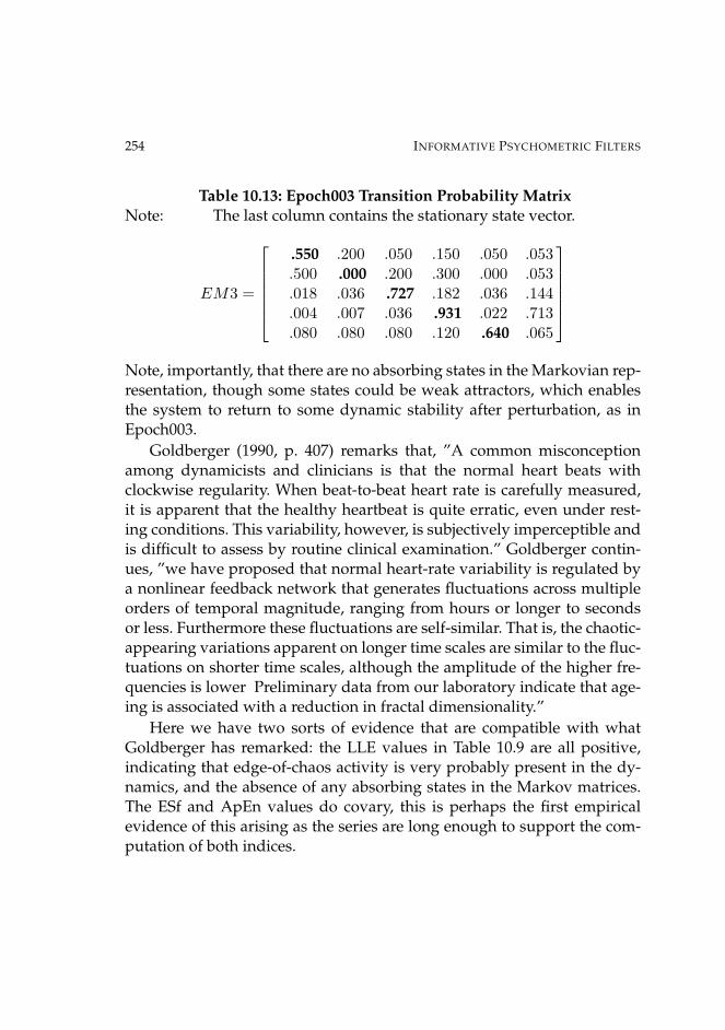
254 INFORMATIVE PSYCHOMETRIC FILTERS
Table 10.13: Epoch003 Transition Probability MatrixNote: The last column contains the stationary state vector.
EM3 =
.550 .200 .050 .150 .050 .053.500 .000 .200 .300 .000 .053.018 .036 .727 .182 .036 .144.004 .007 .036 .931 .022 .713.080 .080 .080 .120 .640 .065
Note, importantly, that there are no absorbing states in the Markovian rep-resentation, though some states could be weak attractors, which enablesthe system to return to some dynamic stability after perturbation, as inEpoch003.
Goldberger (1990, p. 407) remarks that, ”A common misconceptionamong dynamicists and clinicians is that the normal heart beats withclockwise regularity. When beat-to-beat heart rate is carefully measured,it is apparent that the healthy heartbeat is quite erratic, even under rest-ing conditions. This variability, however, is subjectively imperceptible andis difficult to assess by routine clinical examination.” Goldberger contin-ues, ”we have proposed that normal heart-rate variability is regulated bya nonlinear feedback network that generates fluctuations across multipleorders of temporal magnitude, ranging from hours or longer to secondsor less. Furthermore these fluctuations are self-similar. That is, the chaotic-appearing variations apparent on longer time scales are similar to the fluc-tuations on shorter time scales, although the amplitude of the higher fre-quencies is lower Preliminary data from our laboratory indicate that age-ing is associated with a reduction in fractal dimensionality.”
Here we have two sorts of evidence that are compatible with whatGoldberger has remarked: the LLE values in Table 10.9 are all positive,indicating that edge-of-chaos activity is very probably present in the dy-namics, and the absence of any absorbing states in the Markov matrices.The ESf and ApEn values do covary, this is perhaps the first empiricalevidence of this arising as the series are long enough to support the com-putation of both indices.

PERRON-FROBENIUS AT THE EDGE OF CHAOS 255
Higher Order Statistics, bESf
The series are long enough to permit some exploratory analyses using thehigher-order bispectral bESf matrices, that were introduced by Gregsonand Leahan (2003). To emphasise, the bold-face entries are within the ran-dom surrogate 95% c.i. ranges. Each triangular matrix of the b(m,n) seriesof triples, m < n, is written as
b(1,2) b(1,3) b(1,4) b(1,5) b(1,6)b(2,3) b(2,4) b(2,5) b(2,6)b(3,4) b(3,5) b(3,6)b(4,5) b(4,6)b(5,6)
Table 10.14: bESf values for Epoch001
EPb1 =
-.4017 −.5075 −.3283 −.5455 −.4801−.5263 −.4999 −.4311 -.4192−.3482 −.3372 −.4440−.5771 −.3287−.4520
There is little sign of random variations here, in what is essentially ahigher-order high-pass filtering, on the higher-frequency fluctuations ofthe inter-beat-interval. It is expected that Epoch002 will be much the same,but Epoch003 disturbed. Computing in the same fashion:
Table 10.15: bESf values for Epoch002
EPb2 =
−.3010 −.4986 -.4277 −.5426 -.4179−.3064 −.3381 −.4643 −.3507−.5201 −.4423 -.4297−.4456 -.4056-.4205
This EPb2 series has more noise than EPb1 in it.

256 INFORMATIVE PSYCHOMETRIC FILTERS
Table 10.16: bESf values for Epoch003
EPb3 =
−.3042 −.4512 −.4088 −.3165 −.5310−.4105 −.3483 −.4247 -.3785-.4338 −.2446 −.4811-.4056 −.3587−.3967
The noise has now moved from its location in the previous two matrices.As remarked in our previous work on series of this nature (Gregson, 2003),the bESf matrices are the off-diagonal parts of square skew-symmetric ma-trices, so their eigenvalues are computable and all real. They provide an-other way of examining shifts in the dynamics with stimulus disruption;here, dominant stimuli to the cardiac system are breathing rhythms.
Table 10.17: Eigenvalues for bESf for all three Epochs
Eigenvalue Epoch001 Epoch002 Epoch003[1] -2.6538 -2.5340 -2.3636[2] -0.2590 -0.1971 -0.2269[3] 0.2442 0.1735 0.2032[4] 0.1481 0.1059 0.1366[5] -0.1450 -0.0431 -0.0621[6] -0.0147 -0.0264 -0.0451
It is clear that the dynamics of all three epochs are not identical and thesmall differences between the first and third epochs, on the one hand, andthe second, are expressed in the lesser [2,3,4] eigenvalues in Table 10.17.
Subdividing the Third Epoch.
Before computing, it is illuminating to examine the graphs of each of thethree series, but after they have been high-pass filtered. Figures 10.1, 10.2,

PERRON-FROBENIUS AT THE EDGE OF CHAOS 257
Figures 10.4, 10.5, 10.6: The three cardiac i.b.i. seriesRaw data after high-pass filtering
10.3 show the results, the vertical axis scales of the graphs differ to accom-modate the different ranges of variability.
We now break the third epoch into the first 160 inter-beat-intervals,then the next 120, then the remaining 106, and compute for each sepa-rately; that is, three subseries in sequence. The anomalous subseries, fromthe high-pass filtered graphs, is the middle one (Epoch032), and the firstand third can be considered as controls and should resemble Epochs 001and 002.
Computationally we may run into difficulties with the shorter series,that may be insufficient to produce stable estimates of LLE or ApEn. Forthe ESf estimates in Table 10 δy = .01. These should all be compared with

258 INFORMATIVE PSYCHOMETRIC FILTERS
Epoch003 in Table 10.9.
Table 10.18: descriptive statistics of Epoch003 partitioned
measures Epoch031 Epoch032 Epoch033min 300 304 718max 910 1011 917
mean 738.56 715.63 810.31s.d. 99.48 161.23 39.88
Skewness -2.904 1.118 0.162Kurtosis 8.931 0.587 0.182intercept 771 576 846
slope -.417 2.334 -0.698LLE .095 .066 .116
Low pass LLE .039 .038 .118High pass LLE .061 .011 .031
ESf -.4567 -.2566 -.3114ApEn .4765 .4064 .4689
The variations in ESf are greater than in ApEn, so it is in this context a moresensitive measure of the destabilization induced in the middle subseriesEpoch032 by a temporary burst of a shallow fast breathing rhythm.
Self-Similarity at Different Scales
If the time series have fractal properties, and it is suggested by variousauthors that they would have, then, if we create a coarser series from thegiven data by halving the frequency of data points, we should get sub-stantially the same statistical parameters from the analyses in the previoustables. That method is, in fact, called multiscale entropy analysis (Costa,Goldberger and Peng, 2002). As Epoch001 seems to be the most stable, it isthis series only that we should employ to check this aspect of the dynam-ics.

PERRON-FROBENIUS AT THE EDGE OF CHAOS 259
Defining
∀m; xm(j) = (x(i) + x(i− 1))/2, j = mod2(i)
so that the half frequency series length n/2 is 193 double i.b.i.s longthe quarter frequency series is 96 long, and the eighth frequency seriesis 48 long, then ESf(1/2) = -.3111, ESf(1/4) = -.3194, and ESf(1/8) = -.1621.
Multiple analyses on sample series
Comparing the behaviour of different indices computed on successivesubsamples of time series is comparing the actions of different filters. Afilter may or may not preserve metric information, linear statistics suchas autocorrelations or moments do, and the various entropy-based indicesdo not, but are based in information theory. A filter may reject some in-formation and may also transform it or create spurious information if itsinbuilt assumptions are not compatible with the data structure. If the basicprocesses being studied are not stationary, then a filter that only representssome of the information present may vary in what it captures.
As an illustration of the variability that can be found under conditionsthat might reasonably be thought to be stable and even tranquil, Table10.19 shows one series collected under meditation conditions. The valuesare here expressed as interbeat intervals (i.b.i) in 100ths of a second. Thisseries could be taken as one sort of base rate situation. The various mea-sures are not usually all computed on the same data set and show somemutual disagreements. All entropy-based measures I have seen have in-built tuning parameters to be set in their computation and their settingscan critically affect the performance of the measures, that is filters, as pro-cess identifiers (Richman and Moorman, 2000).
The relative utility of the various measures is not simply decided, asthey reflect different properties of the nonlinear dynamics. We can say,using the LLE as the basic criterion, that all the series are chaotic, to a smalldegree, and that the largest Lyapunov does vary a bit over time in whatmay be psychophysiologically interpreted as a stable process, as has been

260 INFORMATIVE PSYCHOMETRIC FILTERS
reported in our previous work (Gregson and Leahan, 2003). ESf does havea stronger relation to LLE than ApEn, which is not surprising because ESfuses more series information to construct its values.
Figures 10.7, 10.8, 10.9: The raw data of Meditation blocks 1, 4 and 10Showing non-stationarity. Vertical scales vary.
Each of the ESf values has been checked against the 95% confidenceinterval found from a set of 50 random surrogate series, and shown to be

PERRON-FROBENIUS AT THE EDGE OF CHAOS 261
outside and above the associated random interval.
The higher-order bESf matrices for two selected blocks are shown inTables 10.20 and 10.21. As previously, the bold-face entries are within therandom surrogate 95% c.i. The mixture of chaotic and random componentsof the higher-order dynamics again appears. There is a possible resem-blance between Tables 10.8 and 10.13, interestingly as one is drawn fromAustralia and the other from the USA, they are independent analyses.
Table 10.19: Descriptive statistics of Meditation seriesThis series of ECG data is taken from the PhysioNet archives.
Block LLE mean Kurt ESf D2 H ApEn1-400 +.1123 68.88 -0.572 -.4341 1.813 .1866 1.020
401-800 +.1062 71.53 -0.999 -.4678 1.853 .1472 0.950801-1200 +.1198 73.51 -1.287 -.4594 1.819 .1805 0.829
1201-1600 +.0986 73.48 -1.135 -.4529 1.801 .1987 0.9531601-2000 +.1285 73.70 -0.973 -.4837 1.767 .2333 0.9492001-2400 +.1513 74.63 -1.092 -.4935 1.832 .1684 1.0292401-2800 +.1224 74.12 -1.047 -.4238 1.807 .1931 0.9542801-3200 +.1496 75.02 -1.188 -.4359 1.810 .1934 0.8723201-3600 +.1284 73.38 -0.622 -.4857 1.859 .1411 1.0533601-4000 +.1254 75.85 -0.403 -.4185 1.769 .2314 1.111
– – – – – – – –cftv .129 .025 .300 .056 .016 .155 .082regr 1 63.53 -2.02 -0.34 -0.02 0.06 0.15corr 1 .544 -.116 -.214 -.010 .034 .030
Key: Block: beats in sequence. LLE: largest Lyapunov exponent. mean: av-erage i.b.i. Kurt: kurtosis. ESf: entropic analogue of Schwarzian derivative.D2: fractal dimensionality. H: Hurst index. ApEn: approximate entropy(k = 10, δ = .02). cftv: coefficient of variation (σ/|µ|). regr: slope of regres-sion of variable on LLE. corr: product-moment correlation of LLE withvariable.
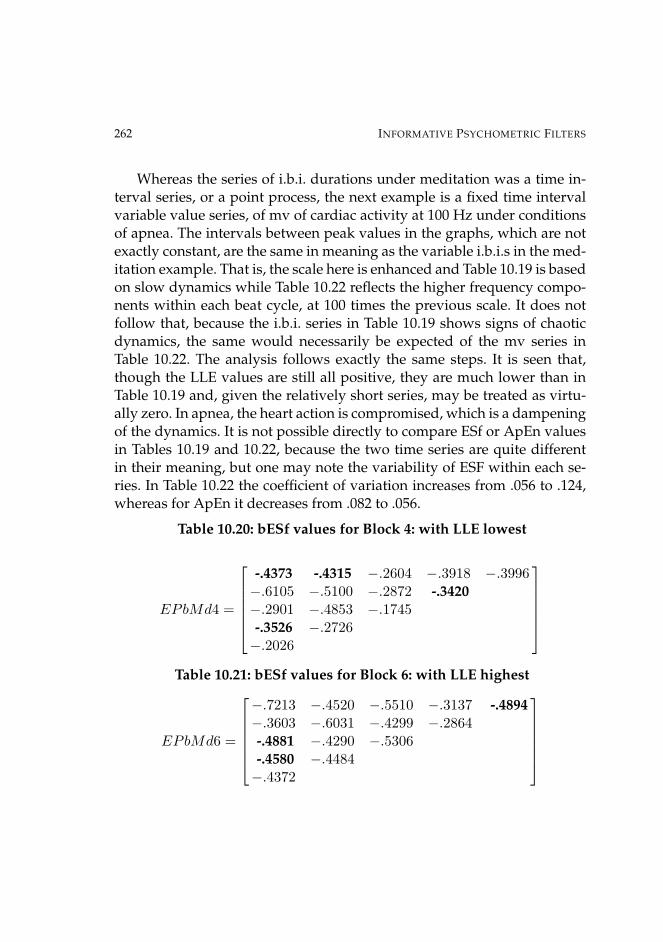
262 INFORMATIVE PSYCHOMETRIC FILTERS
Whereas the series of i.b.i. durations under meditation was a time in-terval series, or a point process, the next example is a fixed time intervalvariable value series, of mv of cardiac activity at 100 Hz under conditionsof apnea. The intervals between peak values in the graphs, which are notexactly constant, are the same in meaning as the variable i.b.i.s in the med-itation example. That is, the scale here is enhanced and Table 10.19 is basedon slow dynamics while Table 10.22 reflects the higher frequency compo-nents within each beat cycle, at 100 times the previous scale. It does notfollow that, because the i.b.i. series in Table 10.19 shows signs of chaoticdynamics, the same would necessarily be expected of the mv series inTable 10.22. The analysis follows exactly the same steps. It is seen that,though the LLE values are still all positive, they are much lower than inTable 10.19 and, given the relatively short series, may be treated as virtu-ally zero. In apnea, the heart action is compromised, which is a dampeningof the dynamics. It is not possible directly to compare ESf or ApEn valuesin Tables 10.19 and 10.22, because the two time series are quite differentin their meaning, but one may note the variability of ESF within each se-ries. In Table 10.22 the coefficient of variation increases from .056 to .124,whereas for ApEn it decreases from .082 to .056.
Table 10.20: bESf values for Block 4: with LLE lowest
EPbMd4 =
-.4373 -.4315 −.2604 −.3918 −.3996−.6105 −.5100 −.2872 -.3420−.2901 −.4853 −.1745-.3526 −.2726−.2026
Table 10.21: bESf values for Block 6: with LLE highest
EPbMd6 =
−.7213 −.4520 −.5510 −.3137 -.4894−.3603 −.6031 −.4299 −.2864-.4881 −.4290 −.5306-.4580 −.4484−.4372

PERRON-FROBENIUS AT THE EDGE OF CHAOS 263
The original data did not specify if medication was being used whenthese records were obtained, so it is not possible to partial out any causal-ity, digitalis is often used to control arrhythmias, and these series are quiteregular and have a recurrent defined periodic spectrum, with no evidenceof tachycardia.
Here, the ApEn values are very stable, but the ESf shows fluctuations,it uses higher-order derivatives and these appear to play a role that is notdetected by ApEn. The difference in the LLE values between Tables 10.19and 10.22, suggesting that the slow i.b.i. series are chaotic, but the highfrequency mv series within the i.b.i.s are not chaotic, is not novel, but hasbeen considered for brain dynamics at different levels (Wright and Liley,1996; Gregson, 1997).
Tables 10.23 and 10.24, unlike Tables 10.20 and 10.21, are generated bythe high frequency dynamics that produce the p,q,r,s fluctuations in mv ineach cycle near the peak. The values within the triangular bESf matricesare lower for this (fast) series, than for the (slow) meditation i.b.i.s. There islittle evidence of any random components here, so the process is nonlinearbut not chaotic at a lower (slow) level, taking all the evidence in Table 10.24together.
Panic Pre-dynamics
The findings of Gorman & Sloan (2000) on the importance of heart ratevariability have already been mentioned and it is important to note thatsuch variability itself is complex and has sources that are usually con-founded without appropriate statistical analyses (Chon, Zhong, Wang, Juand Jan, 2006.
But the question remains, what measures of variability in time seriesare most relevant? Tucker, Adamson & Mirander (1997) use power spec-tral analysis. That presumes linearity and dynamic stationarity, and thusfilters out aspects of the dynamics that are known to be present in normalcardiac activity, that is, in fact, edge-of-chaos (Winfree, 1987). So far as can

264 INFORMATIVE PSYCHOMETRIC FILTERS
Figures 10.10, 10.11, 10.12: The raw data of Apnea mv blocks 1, 5 and 7Illustrating cyclic variation. Vertical scales vary

PERRON-FROBENIUS AT THE EDGE OF CHAOS 265
Table 10.22: Descriptive statistics of Apnea mv seriesThis series of ECG data is taken from the PhysioNet archives.
Block LLE mean Kurt ESf D2 H ApEn1-400 +.0246 .0009 13.81 -.4771 1.863 .1373 .383
401-800 +.0328 .0043 18.90 -.3427 1.741 .2594 .326801-1200 +.0481 -.0021 19.25 -.4562 1.854 .1458 .344
1201-1600 +.0163 .0013 19.02 -.3357 1.900 .1003 .3231601-2000 +.0625 -.0043 13.45 -.4150 1.860 .1404 .3632001-2400 +.0516 .0032 17.69 -.4270 1.841 .1594 .3712401-2800 +.0645 .0002 13.49 -.4413 1.876 .1244 .3702801-3200 +.0387 -.0047 14.85 -.3303 1.863 .1370 .3593201-3600 +.0439 .0041 15.24 -.4348 1.824 .1762 .3793601-4000 +.0262 -.0077 16.19 -.4430 1.835 .1648 .370
– – – – – – – –cftv .375 8.070 .138 .124 .022 .262 .056regr 1 -.006 -58.355 -1.021 .135 -.131 .436corr 1 .0245 .4001 -.3071 .0513 .0498 .3349
Key: As Table 19. For ESf k = 10, δ = .0025
Table 10.23 bESf values for Block (3) with ESf high
EPbApn3 =
−.3243 −.3653 −.1395 −.2625 −.1647-.3043 −.3076 −.2130 −.4101−.4350 −.2807 −.3520−.1827 −.3461−.1582

266 INFORMATIVE PSYCHOMETRIC FILTERS
Table 10.24: bESf values for Block (8): with ESf lowest
EPbApn8 =
−.3027 −.4218 −.2350 −.5100 −.3702−.3523 −.2472 −.5195 −.3288−.4834 -.4099 −.4909−.2613 −.5160−.1878
be deduced from literature reviews, variability is in most studies simplyequated with Gaussian variance about a mean heart rate.
Though the focus of this intended study is on heart rate variability dur-ing periods when patients are not having panic, there are still other con-ceptual difficulties to be noted. Margraf and Ehlers (1992, p. 154) remarkthat it is inadequate to ”dichotomize the subjects’ complex responses sim-ply into panic or not panic”. They note that it is not the case that during apanic attack a subject’s heart rate always increases. ”In addition to beingprone to biases, relying on the artificial dichotomous variable ’panic/notpanic’ entails a considerable loss of information compared to the measure-ment of continuous variables.” The same argument can be applied to thetime series analysis of cardiac activity, if the latter is only encoded as ”ele-vated/normal” in the local mean rate.
Margraf and Ehlers conclude (1992, p. 224) that, ”a pure medical ill-ness approach to panic has been shown insufficient, possible biologicalvulnerabilities have been revealed only for subgroups, and the necessity ofa psychophysiological perspective has been underlined the integration ofdifferent levels of analysis is a basic problem of all modern neuroscience.Rather than biological or cognitive reductionism a true psychobiologicalperspective is needed.”
Notes
The statistical calculations were made partly by using SANTIS softwarefrom the Physiology Department of the University of Aachen and by the

PERRON-FROBENIUS AT THE EDGE OF CHAOS 267
author’s own programs in Linux Fort77, and in Mathematica. Dr Pincuskindly provided code of his Approximate Entropy program which wasrewritten into Linux. The time series in the second part were drawn fromthe PhysioNet Archives.
Appendix
For µ = .735 the eigenvalues of LS are, in complex form:
1.0, .715 + .1009i, .715− .1009i, .645 + .1645i, .645− .1645i
The dimensionality of the embedding space of the Shilnikov attractoris three. A perspective picture of its trajectory is given by Mitchener& Nowak (2004, p. 704). The formal mathematics of the Shilnikov phe-nomenon are given by Wiggins (1990, pp. 573, 602). It arises in the dy-namics near an orbit homoclinic to a fixed point of saddle-focus type in athird-order ordinary differential equation. The equation can be of the form
x = ρx− ωy + P (x, y, z),y = ωx+ ρy +Q(x, y, z),z = λz +R(x, y, z).
where P,Q,R are complex. The eigenvalues are given by ρ± iω.A deeper mathematical treatment is given by Wiggins (1988, p. 227
et seq), wherein it is noted that the attractor possesses a 2-dimensionalstable manifold and a 1-dimensional unstable manifold. The time of flightbetween the two attractors is a function of λ.
The dynamics in the local regions of saddle-nodes, of which this canbe an example, are treated qualitatively by Shilnikov, Shilnikov, Turaev& Chua (1998). A further treatment of the role of eigenvalues in the sub-system identification of metastable Markov systems has recently been re-viewed by Huisinga, Meyn and Schutte (2004).


Chapter 11
Appendix: NonlinearPsychophysical Dynamics
This appendix summarises some algebraic properties used in nonlinearpsychophysics with reference to their contextual literature in pure math-ematics. It enlarges on some material presented graphically in Chapter 1,and drawn on particularly in Chapters 3, 7, 8 and 10.
Alternative representations of the dynamics in real time:
(1) Julia sets of the dynamics, with coordinates the startingpoints Y (Re, Im)0 of the recursive iterations which yieldthe trajectories; attractor basins and self-similarities dis-played with magnification.
(2) Dynamic partitions of the system’s parameter space; localregions associated with attractor characteristics. Coordi-nates are the equation’s fixed parameters, not the internalvariable.
(3) Mappings indicating homoclinic and heteroclinic orbits,distinguishing real and complex spaces, and Poincarespace sections.

270 INFORMATIVE PSYCHOMETRIC FILTERS
(4) Trajectories as parallel time series of Real and Imaginaryparts of the system variable Y , recurrence maps, and al-ternative series based on transformations into polar coor-dinates.
(5) Symbolic dynamic encodings of the time series createdby discrete partitioning into Markovian state variables.These are the basis used here to identify arpeggio-likesubsequences.
(6) Response surfaces of terminal values of the trajectoriesover the parameter space. These come in pairs and onein the Reals corresponds most closely to psychophysicaldata from the perspective of an external observer. Surfacesmay be differentiated and the derivatives used to estimateresponse latency frequency distributions via Jacobians.
(7) Cross-entropy maps from input parameter values to Realparts of the output at a fixed number of iterations. Usedto assess information loss in stimulus-response pairings.
(8) Time series of convoluted trajectories, with variable gainparameters, matching in meaning < 4, 5, 6, 7 >.
A general mathematical results which Milnor (1992) draws on is that anycubic polynomial map from the complex numbers C to C is conjugate,under a complex affine change of variable, to a map of the form
z 7→ f(z) = z3 − 3a2z + b [11.1]
and we note that Γ in nonlinear psychophysical dynamics (NPD)(Gregson,1988, 1992, 1995) which is defined as
Γ : Yj+1 = −a(Yj − 1)(Yj − ie)(Yj + ie), i =√−1, j = 1, ..., η
[11.2]falls into this family.
A more general form which exemplifies the structural questions in-volved is to rewrite Γ as its generic family
Γ : Yj+1 = f(π, ..., πζ , Yj−k(Re, Im), Yj(Re, Im))

APPENDIX: NONLINEAR PSYCHOPHYSICAL DYNAMICS 271
in which π is any parameter, and the presence of an indeterminate num-ber of complex eigenvalues has to be allowed a priori. The dynamics varycritically with the eigenvalue structure (Ilyashenko & Li, 1999). In [11.2]we have simply ζ = 2 and one complex eigenvalue, in other words, acomplex conjugate pair. The subscript k allows for delay, and in [11.2] iszero, but has been 1 in some cases considered (Gregson, 1995, 1998). Theterminating parameter η in [11.2] is not a necessary part of the definition;it is merely an arbitrary limit to the trajectory.
The parameters π are usually taken to be scalar constants, but inΓc convolutions become variables under some definable conditions. Theshape of the plot of Y (Re)/a is similar to a cumulative normal ogive, andalso to
v(x) =
0, x ≤ 0,sin2 π
2x, 0 ≤ x ≤ 1,1, x ≥ 1.
(Daubechies, 1992, p.74).
If, instead, the situation were to be modelled in stochastic dynamics,then the nearest statistical model would be the random walk plus noise hier-archical form (Atkinson, 1998)
yt = αt + εt εt ∼ N(0, σ2ε ) [11.3]
εt+1 = αt + ηt ηt ∼ N(0, σ2η) [11.4]
where y replaces Y (Re) in the NPD structure, and α replaces a in Γ. Boththe nonlinear dynamical convoluted system and the stochastic randomwalk system use a single time counting unit, as usually presented, bothfor the driving and the response parts, which is t in [11.3,11.4] above andj in [11.2].
Consider a single channel psychophysical process mediated by a lo-cally destabilised Γ trajectory (Gregson, 1988). There are three successivetime segments called epochs,
t = 1, ..., n1, n1 + 1, ..., n2, n2 + 1, ..., N

272 INFORMATIVE PSYCHOMETRIC FILTERS
The stimulus is only made to be present in the middle time segment, ofduration n2 − n1. The gain settings are ag in the first and third epochs,and af in the middle epoch. To reflect familiar psychological terms, g is forground and f is for figure. For the ground condition in epochs 1,3 Γg is[11.2] with a = ag, and for the stimulus epoch Γf is [11.2] with a = af .
Converting to polar coordinates, with starting values Y0(Re,Im), set
x = Y (Re), w = (Y0(Im).10c)−1, y = w(Y (Im).102c) [11.5]
thenr = (x2 + y2)1/2, tanθ = y/x [11.6]
are the renormed polar coordinates required.For example, in studying the dynamics of rhythmic motion, Treffner
and Turvey (1996) use
dφ/dt = ∆ω − a sin(φ)− 2b sin(2φ) +√Qζt [11.7]
to predict equilibria and fluctuations in symmetry breaking during handcoordination tasks.
In general, the family of maps
x 7→ x+ µ+ ε cos2πx = f(x, µ, ε), x ∈ R1, ε ≥ 0 [11.8]
where points in R1 that differ by an integer so that [11.8] can be regardedas a map defined on the circle S1 = R1/Z is a generator of Arnol’d tonguesdue to the presence of terms in O(ε3). So far, there exists no formal proofthat [11.2] with periodicity in a resembles a case of [11.8], but see Chavoya-Aceves et al (1985)1
Milnor (1992, p.11) illustrates this point by comparing what he calls”pointed-swallow” configurations in Arnol’d tongues with arch configu-rations in cubic maps.
1 Arnol’d tongues can be generated also by the sine-map of the circle, which is
Yn+1 = Yn + a + b sin2πYn(mod1),
effectively the same form as [11.8].

APPENDIX: NONLINEAR PSYCHOPHYSICAL DYNAMICS 273
Let a = f(α| sin(κπt)|), 2.5 < a < 5.0, t ≡ j within the stimulus epoch.Here κ determines the periodicity and α determines the amplitude, whichhas to be constrained to keep the dynamics within the attractor basin of Γ.
——————————————————-Table 11.1: Local behaviour of output after a sinusoidal peak input
rt for various e after 50 interations of Γe→ .2 .25 .3 .35a ↓
4.3920 2.5663 0.9946 0.7954 4.92954.6789 3.9077 2.5827 1.4365 6.52424.8790 1.6367 2.4472 5.6596 13.95064.9842 0.7577 4.2730 9.4996 23.47244.9904 0.9428 4.8962 18.8983 55.20534.8973 1.9336 8.3213 23.8296 66.68274.7086 2.2313 2.0982 52.4784 203.61654.4319 3.4945 0.9261 10.1625 54.1295
——————————————————-Some of the results here have been foreshadowed by Ott, Grebogi and
Yorke (1990). They write: ”The behaviour of the response system dependson the behaviour of the drive system, but the drive system is not influ-enced by the response system. We have split the drive system into twoparts. The first part represents the variables that are not involved in driv-ing the response system, and the second part represents the variables thatare actually involved in driving the response system.” In cascaded Γ nota-tion this is exactly the same thing as putting ak+1 = f(Yη|k(Re)) (Gregson,1995, gives detailed examples).
Guided by psychophysical considerations, the situation chosen for ex-ploration involves setting up a convolution of one Γ trajectory onto a cas-cade of a second series of Γ trajectories, where the first Γ1 is quasiperiodicor chaotic in the reals, and using
a2 = α+ βY1 (Re) [11.9]
where α and β are real positive scalars to make the range of Y2(Re) liewithin stable limits,, as a2 is input to Γ2 with its η2 not less than 4. This

274 INFORMATIVE PSYCHOMETRIC FILTERS
convolution, ΓC = Γ2(Γ1) in operator notation, with settings of e chosento give autonomous dynamics beyond the first bifurcation for each Γ, isof potential interest and psychophysically possible. Such convoluted andcascaded series are also compatible in principle with what is known aboutpathways between the hippocampus and the frontal cortex (Halgren &Chauvel, 1996).
For illustration consider two examples, for complex and for polar tra-jectories. Suppose that a1 = 4.1251, e = .447226, α = 2.13 and β = 2.55,then Y1(Re) runs into quasiperiod 8 with roughly to the first decimal placethe sequence .9•, .3•, .8•, .5•, .9•, .2•, ..., (the symbol • in each step indi-cates omitted digits in the recursion of Γ). The a2 series then starts with4.30•, 3.25•, 3.78•, 3.49•, 3.73•, 3.68•, .. and the generated Y2(Re) serieswith η2 = 5 runs onto quasiperiod 8 with .9•, .7•, .8•, .6•, .9•, .7•, .9•, .6• ...But in the first phase of the convolution the largest Lyapunov exponent isnegative, for the Y1(Re) series, it moves from positive to negative for thepolar r1 series, it is positive and slowly stabilises for Y2(Re) and is positiveand unstable for polar r2.
A second case where the dynamics are very near to explosion andhave become aperiodic can be created by setting a1 = 4.132503, e =.447226, η1 = 360, then α = 2.13, β = 2.55, and η2 = 4, which createsan interesting series in Y2(Re). The Y1(Re) series is quasiperiodic 8, with.9•, .3•, .8•, .5•, .9•, .2•, .8•, .6•, .. and to characterise the Y2(Re) or r2 seriesa variant of symbolic dynamics is useful (Kantz and Schreiber, 1997).
From examination of the generated Y2(Re) series for t = 1, ..., 359 aconvenient partitioning of Y to create an X variable is made (the set ofvalues X become the states of a Markov process, as are used in the box-counting methods for mapping attractors; see Kreuzer, 1987).
and a series is then of the formX1m1X2m2X3m3....Xkmk..wheremk =0, ...,∞ is the number of successive Ø values of X in the inter X intervalXkXk+1,X ∈ A,B,C,D,E, F. For example a continuous segment of theseries is found to read as
.......E3C3F1 C1C3E1A1C3F1D1C3D1B1C3F1 C1C3E1A1C3F1→C1C3E2C3F1 C1C3E1A1C3F1D1C3... [11.10]The → indicates unbroken continuity. The subsequence set in boldface

APPENDIX: NONLINEAR PSYCHOPHYSICAL DYNAMICS 275
——————————————————-Table 11.2: Partitioning of input to create a symbolic variable
if 0 < Y < .61 X ≡Øif .61 < Y < .62 X ≡ Aif .62 < Y < .63 X ≡ Bif .63 < Y < .64 X ≡ Cif .64 < Y < .65 X ≡ Dif .65 < Y < .66 X ≡ E
and if Y > .66 X ≡ F——————————————————-
may be regarded as an arpeggio-like event Φ. There are two time serieshere which may provide evidence of near-chaos or chaotic dynamics; theinter-Φ-interval frequency distribution and its series, its first two terms be-ing 16 and 14 Xm steps, and the series of m values, at a finer resolution intime, which is running as
.....3,1,1,3,1,1,3,1,1,3,1,1,3,1,1,3,1,1,3,1,3,2,3,1,1,3,1,1,3,1,1.. [11.11]which is almost period 3.
The symbolic dynamics just constructed rest on only the Y2(Re) series;if instead the associated polar modulus r2 series is used, not quite thesame patterns merge. The comparison analysis is performed on the samesegment of the trajectory of Γ2. Comparing with [11.10], but for polar r2,reading the iterations from the same time point onwards,
...EC2C2FF1C1A2E1A1C3FFFFC2FFF1FC2FEF1FC2F→F1C1CC2E1AFCD2F1C1C2.. [11.12] from which it is not possible toidentify any recurrent Φ within the same time window. The new sequenceof m values, corresponding to [11],is now
....2,2,0,1,1,0,2,1,1,3,0,0,0,0,2,0,0,0,1,0,2,0,0,1,0,2,0,1,1,1,0,2,0,0,0,2,..[11.13]Making a change in e from 0.447226 to 0.47227 is a sufficient example, stilljust within stability retaining a2 unchanged.
For Y (Re) over the same range of iterations as before we now have(compare [11.10]):
...E3C3E1A1C3F1C1C3E3C3 F1B1C3E1A1C3→

276 INFORMATIVE PSYCHOMETRIC FILTERS
F1B1C3FB1C3 F1B1C.. [11.14]and again there is the emergence of an arpeggio Φ but not the same one asin [11.10]. The m series corresponding to [11.11] is like
...3,3,1,1,3,1,1,3,3,3,1,1,3,1,1,3,1,1,3,1,1,3,1,1,... [11.15]which is apparently quasiperiodic 3, rather like [11.10]. Repeating the exer-cise for the corresponding symbolic dynamics of polar modulus r2 yields(compare [11.12])
......EE1FC3E1A1CF1FF1CFCE2E2FCC1 FF1B1C2FEFA1→C2 FF1B1C3F1BFCF1 FF1BFCF1.. [11.16]and the weak emergence of a Φ is seen. The correspondingm series is now
....0,1,0,3,1,1,0,1,0,0,0,0,2,2,0,0,1,0,1,1,2,0,0,0,1,2,0,1,1,0,1,0,0,0,1,0,1...[11.17]which appears to be locally aperiodic.
It is immediately obvious that the autocorrelation structure of the re-sponse Y2(Re) series can be different for the two cases, and the autocor-relation structure will be related to the largest Lyapunov exponent. Forillustration, recomputing the last example given, in [11.14-11.17], witha = 4.132503, e = .447227, which is period 8 approximately during thedriving stage, gives (for comparison with [11.14]) for Y2(Re),
......EFC1 CF2DF2A1 CF2EFC1 CF2DFA CF2EFB1 CF2DFA→CF2EFB1 CF2DFB CF2EFB1CF... [11.18]and in this string we can identify two Φ which may later coalesce. Thecorresponding m series (compare [11.17]) is thus
0,0,1,0,2,0,2,0,2,0,0,1,0,2,0,0,1,0,1,0,0,1,0,2,0,0,1,0,2,0,0,1,0,2,0,0,1,0,2,.[11.19]which is period 5 after it stabilizes. The new polar r2 series is quasiperiodic8 and quite uninteresting.
The definition of mutual information I(X,Y ) takes a general form,with ∀i xi ∈ X, ∀j yj ∈ Y , and bivariate summation implicit
I(X,Y ) =T∑i=1
T∑j=1
pXY (xiyj)log2(
pXY (xiyj)pX(xi)pY (yj)
)[11.20]
The form of [11.20] extends to cover the case where one series is lagged

APPENDIX: NONLINEAR PSYCHOPHYSICAL DYNAMICS 277
onto itself, or delayed onto another realization of the same series, by writ-ing (Abarbanel, 1996, p.28), where the lagged delay is θ recursive steps ofthe map,
I(θ) =T∑n=1
(p(yn, yn+θ)log2(
p(yn)p(yn)p(yn+θ)
)[11.21]
and we may then proceed to find the θ which maximises I(θ) for agiven realization of the process. For example, if [11.14] is repartitionedat values Y (Re) = .54,.57,.62,.63,.64,.66 to give seven states over the con-tinuum 0,1 then it is seen, as the system is stationary in its parame-ters, that it is near equilibrium with a stationary state probability vector.362,.139,.140,.008,.137,.002,.108. It is this vector which is stochastically ex-ternally observable behaviour; the actual values depend on where the ar-bitrary partitions on Y are set and how many are chosen. The basic infor-mation definition H = −
∑7i=1 pilog2(pi) can be computed for the vector.
A slightly different exploration of the Y2(Re) series, for various η2, isused in Table 11.3. It is suspected that the information of the Y2(Re) fre-quency distribution is a function of η2, from some precedents. For Table
—————————————————Table 11.3: Information capacity of the Y2,η(Re) distributions
For various iterations, of the original and the first and second differenced series.η2 H[Y (Re)] H∆1[Y (Re)] H∆2[Y (Re)]2 2.502 1.419 1.3764 2.505 1.470 1.4185 2.508 1.423 1.4226 2.500 1.367 1.3077 2.529 1.447 1.4578 2.500 1.369 1.307
10 2.500 1.351 1.30911 2.501 1.351 1.30915 2.501 1.326 1.312—————————————————

278 INFORMATIVE PSYCHOMETRIC FILTERS
11.3 the Y2(Re) range has been partitioned into 10 equal steps of 0.1; if thedistribution were rectangular then H would be 3.322 (= log210). Actually,it is not ever that, and for Y1(Re) H = 2.500, so, except for an apparentirregularity at η2 = 7, the information is not much altered by the con-volution, though the actual distribution of Y values is altered. The firstLyapunov exponent can also reverse sign, and is not the same for the firstand second differences (∆1, ∆2) of the Y2 series.
A relevant comment of Boon and Prigogine (1998, p.4) who write:
Le phenomene musical possede une certaine coherence, in-termediare entre l’aleatoire et le periodique: il y a descorrelations, mais pas de structure strictement deterministe Lamusique possede une symetrie brisee: elle se deroule selon unordre temporel
Notes
(1) The standard notation C, R, Z refers respectively to Complex, Realand Integer domains. The notation of NPD algebra is made to be fullyconsistent with the previous text references given.
(2) The idea of arpeggios Φ in the symbolic dynamics used here appar-ently parallels what are also called isolating segments in chaotic phasesequences (Wojcik, 1998).

References and Bibliography
Abarbanel, H. D. L. (1996) Analysis of Observed Chaotic Data. New York:Springer-Verlag.
Abraham, N. B., Albano, A. M., Passamante, A. and Rapp, P. E. (Eds.)(1989) Measures of Complexity and Chaos. New York: Plenum Press.
Abrams, D. M. and Strogatz, S. H. (2006) Chimera States in a Ring ofNonlocally Coupled Oscillators. International Journal of Bifurcation andChaos, 16, 21-37.
Aczel, J. (1966) Lectures on Functional Equations and their Applications. NewYork: Academic Press.
Adami, C.,and Cerf, N. J. (2000) Physical complexity of symbolic se-quences. Physica D, 137, 62-69.
Aguirre, L. A., and Billings, S. A (1995) Identification of models for chaoticsystems from noisy data: implications for performance and nonlinearfiltering. Physica D, 85, 239-258.
Ambuhl, B., Dunki, R. and Ciompi, L. (1992) Dynamical Systems and theDevelopment of Schizophrenic Symptoms - An Approach to a Formal-ization. In: Tschacher, W., Schiepek, G. and Brunner, E. J. (Eds.) Self-Organization and Clinical Psychology. Berlin: Springer-Verlag. 195-212.
Amit, D. J. (1989) Modelling Brain Function: The World of Attractor NeuralNetworks. New York: Cambridge University Press.
Andrews, D. F. and Herzberg, A. M. (1985) Data. [Springer Series in Statis-tics.] New York: Springer-Verlag.

280 INFORMATIVE PSYCHOMETRIC FILTERS
Arecchi, F. T. (1987) Hyperchaos and 1/f spectra in nonlinear dynamics:the Buridanus donkey. In: Caianiello, E. R. (Ed.) Physics of CognitiveProcesses. Singapore: World Scientific. 35-50.
Arecchi, F. T., Badii, R. and Politi, A. (1984) Low-frequency phenomena indynamical systems with many attractors. Physical Review A, 29, 1006-1009.
Argoul, F. and Arneodo, A. (1986) Lyapunov Exponents and Phase Tran-sitions in Dynamical Systems. In: Arnold. L. and Wihstutz, V. (Eds.)Lyapunov Exponents. Lecture Notes in Mathematics, No. 1186 Berlin:Springer-Verlag.
Arhem, P., Blomberg, C., and Liljenstrom, H (1999) Disorder versus Orderin Brain Function. Singapore: World Scientific.
Atkinson, A. C. (1998) Discussion of the paper by Hodges. Journal of theRoyal Statistical Society, Series B, 60, 521.
Attneave, F. (1959) Applications of Information Theory to Psychology. NewYork: Holt, Rinehart and Winston.
Baddeley, A. D. and Logie, B.A. (1999) Working memory: The multiplecomponent model. In: A. Miyake and P. Shah (Eds.), Models of work-ing memory: Mechanisms of active maintenance and executive control. Cam-bridge, UK.: Cambridge University Press. 28-61.
Badii, R. and Broggi, G. (1989) Hierarchies of relations between partial di-mensions and local expansion rates in strange attractors. In: Abraham,N. B., Albano, A. M., Passamante, A. and Rapp, P. E. (1989) Measures ofComplexity and Chaos. New York: Plenum Press. 63-73.
Baier, G. and Klein, M. (Eds.) (1991) A Chaotic Hierarchy. Singapore: WorldScientific.
Baker, R. (Ed.) (1992) Panic Disorder: Theory Research and Therapy. NewYork: John Wiley and Sons.
Ball, R. (Ed.) (2003) Nonlinear Dynamics from Lasers to Butterflies. World Sci-entific Lecture Notes in Complex Systems, Vol. 1 Singapore: World Scien-tific.
Bar-Hillel, M. and Wagenaar, W. A. (1991) The Perception of Randomness.Advances in Applied Mathematics, 12, 428-454.

REFERENCES AND BIBLIOGRAPHY 281
Barndorff-Nielsen, O. E., Jensen, J. L. and Kendall, W. S. (Eds.) (1993) Net-works and Chaos - Statistical and Probabilistic Aspects. London: Chapmanand Hall.
Basilevsky, A. and Hum, D. (1977) Spectral Analysis of Demographic TimeSeries: A Comparison of two Spectral Models. In: Barra, J. R., Brodeau,F., Romier, G. and van Cutsem, B. (Eds.) Recent Developments in Statis-tics. Amsterdam: North-Holland.
Berliner, L. M. (1992) Statistics, Probability and Chaos. Statistical Science,7, 69-122.
Berthet, R., Petrossian, A., Residori, S., Roman, B. and Fauve, S. (2003) Ef-fect of multiplicative noise on parametric instabilities. Physica D, 174,84-99.
Bickel, P. J., Ritov, Y. and Ryden, T. (2002) Hidden Markov model likeli-hoods and their derivatives behave like i.i.d. ones. Annales de l’InstitutHenri Poincare, PR 38, (6), 825-846.
Blanchard, F., Maass, A. and Nogueira, A. (Eds.) (2000) Topics in SymbolicDynamics and Applications. London Mathematical Society Lecture Note Se-ries, No. 279. Cambridge: Cambridge University Press.
Blei, R. (2001) Analysis in integer and fractional dimensions. [ CambridgeStudies in advanced mathematics, 71.] Cambridge: Cambridge UniversityPress.
Blei, R. and Janson, S. (2004) Rademacher chaos: tail estimates versus limittheorems. Archiv fur Mathematik, 42, 13-29.
Bohner, M. and Peterson, A. (2001) Dynamic Equations on Time Scales.Boston: Birkhauser.
Boon, J. P. and Prigogine, I. (1998, personal communication) Le temps dansla forme musicale.
Box, G. E. P. and Jenkins, G. M. (1970) Time series analysis, forecasting andcontrol. San Francisco: Holden-Day.
Bowen, R. (1970) Markov partitions for Axiom A diffeomorphisms. Amer-ican Journal of Mathematics, 92, 725-747.
Bower, G. H. and Theios, J. (1964) A learning model for discrete perfor-mance levels. In: Atkinson, R. C. (Ed.) Studies in Mathematical Psychol-ogy. Stanford, Cal.: Stanford University Press. 1-31.

282 INFORMATIVE PSYCHOMETRIC FILTERS
Breakspear, M. (2000) Non-linear coupling underlies alpha rhythm dy-namics in human EEG. International Journal of Psychophysiology, 35, 22.
Brockwell, P. J. and Davis, R. A. (2002) Introduction to Time Series and Fore-casting, 2nd Edn. New York: Springer-Verlag.
Brucoli, M., Carnimeo, L. and Grassi, G. (1995) Discrete-Time CellularNeural Networks for Associative Memories with Learning and Forget-ting Capacities. IEEE Transactions on Circuits and Systems - 1: Fundamen-tal Theory and Applications, 42, 396-399.
Bruhn, J., Ropcke, H., Rehberg, B., Bouillon, T. and Hoeft, A. (2000) EEGapproximate entropy correctly classifies the occurrence of burst sup-pression pattern in anesthesiology. Anesthesiology, 93, 981-985.
Buescu, J. (1997) Exotic Attractors. Basel: Birkhauser Verlag.Buhler, W. K. (1986) Gauss: Eine biographische Studie. Berlin: Springer-
Verlag.Buljan, H. and Paar, V. (2002) Parry measure and the topological entropy
of chaotic repellers embedded within chaotic attractors. Physica D, 172,111-123.
Bunde, A., Kropp, J, and Schellnhuber, H. J. (2002) The Science of Disasters.New York: Springer-Verlag.
Burnham, K. P. and Anderson, D. R. (2002) Model Selection and MultimodalInference. (2nd. Edn. New York: Springer.
Caianiello, E. R. (Ed.) (1987) Physics of Cognitive Processes. Singapore:World Scientific.
Caianiello, E. R. (1989) A study of neuronic equations. In: Taylor, J. G. andMannion, C. L. T. New Developments in Neural Computing. Bristol: AdamHilger. 187-199.
Cao, L., Mees, A. and Judd, K. (1998) Dynamics from multivariate timeseries. Physica D, 121, 75-88.
Carvalho, M. P. de (2002) Chaotic Newton’s sequences. The MathematicalIntelligencer, 24, 31-35.
Chalice, D. R. (2001) How to Differentiate and Integrate Sequences. TheAmerican Mathematical Monthly, 108, 911-921.
Casdagli, M. (1989) Nonlinear prediction of chaotic time series. Physica D,35, 335-356.

REFERENCES AND BIBLIOGRAPHY 283
Casdagli. M. C. (1992) Recurrence plots revisited. Physica D, 108, 12-44.Casdagli, M. and Eubank, S. (Eds.) (1991) Nonlinear Modelling and Forecast-
ing. Reading, MA: Addison-Wesley.Chavoya-Aceves, O., Angulo-Brown, F. and Pina, E. (1985) Symbolic Dy-
namics of the Cubic Map. Physica D, 14, 374-386.Chalice, D. R. (2001) How to Differentiate and Integrate Sequences. The
American Mathematical Monthly, 108, 911-921.Chua, G. (Ed.) (1999) Controlling Chaos and Bifurcations in Engineering Sys-
tems. Boca Raton: CRC Press.Condon, E. U. (1969) Scientific Study of Unidentifed Flying Objects. New
York: US Air Force.Costa, M., Goldberger, A. L. and Peng, C.-K. (2002) Multiscale Entropy
Analysis of Complex Physiological Time Series. Physical Review Letters,89 (6), 068102-1, 068102-4
Cox, D. R. and Lewis, P. A. W. (1966) The Statistical Analysis of Series ofEvents. London: Methuen.
Crounse, K. R., Chua, L. O., Thiran, P. and Setti, G. (1996) Characterizationand dynamics of pattern formation in cellular neural networks. Inter-national Journal of Bifurcation and Chaos, 6, 1703-1724.
Crouzet, F. (1982) The Victorian Economy. London: Methuen.Cundy, H. M. (2000) Snubbing with and without eta. The Mathematical
Gazette, 84, 14-23.Cutler, C. D. and Kaplan, D. T. (1996) Nonlinear Dynamics and Time Series:
Building a Bridge between the Natural and Statistical Sciences. Providence,RI: American Mathematical Society.
Cveticanin, L. (1996) Adiabatic Invariants for strongly nonlinear dynam-ical systems described with complex functions. Quarterly of AppliedMathematics, LIV (3), 407-421.
Daubechies, I. (1992) Ten Lectures on Wavelets. Philadelphia: SIAM.Davies, B. (1999) Exploring Chaos. Reading, Mass: Perseus Books.Dawson, S. P. Grebogi, C., Yorke, J. A., Kan, I. and Kocak, H. (1992) Anti-
monotonicity: Inevitable reversals of period doubling cascades. PhysicsLetters A, 162, 249-254.

284 INFORMATIVE PSYCHOMETRIC FILTERS
de Leeuw, J. (1992) Introduction to Akaike (1973) Information Theory andan Extension of the Maximum Likelihood Principle. In: Kotz, S. andJohnson, N. (Eds.) Breakthroughs in Statistics, Volume I: Foundations andBasic Theory. New York: Springer-Verlag. 599-609.
Demazure, M. (2000) Bifurcations and Catastrophes: Geometry of Solutions toNonlinear Problems. Berlin: Springer-Verlag.
Dickinson, A. (2001) The 28th Bartlett Memorial Lecture. Causal Learn-ing: An associative analysis. Quarterly Journal of Experimental Psychology,54B, 3-25.
Ding, J. and Fay, T. H. (2005) The Perron-Frobenius Theorem and Limitsin Geometry. The Mathematical Association of America Monthly, February2005, 171-175.
Ding, M., Ditto, W. L., Pecora, L. M. and Spano, M. L. (2001) The 5th Exper-imental Chaos Conference. Singapore: World Scientific.
Doyon, B., Cessac, B., Quoy, M. and Samuelides, M. (1993) Control of thetransition to chaos in neural networks with random connectivity. Inter-national Journal of Bifurcation and Chaos, 3, 279-291.
Dunin-Barkowski, W. L., Escobar, A. L., Lovering, A. T. and Orem, J. M.(2003) Respiratory pattern generator model using Ca++-induced Ca++
release in neurons shows both pacemaker and reciprocal network prop-erties. Biological Cybernetics, 89, 274-288.
Edelman, G. M. and Tononi, G. (2001) Consciousness: How Matter BecomesImagination. London: Penguin Books.
Elliot, R.J., Aggoum, L. and Moore, J. B. (1995) Hidden Markov Models. NewYork: Springer-Verlag.
Engbert, R. and Kleigl, R. (2001) Mathematical models of eye movementsin reading: a possible role for autonomous saccades. Biological Cyber-netics, 85, 77-87.
Engel, A. K., Konig, P. and Singer, W. (1991) Direct physiological evidencefor scene segmentation by temporal coding. Proceedings of the NationalAcademy of Sciences of the USA, 88, 9136-9140.
Eykhoff, P. (1974) System Identification: Parameter and State Estimation. NewYork: John Wiley.

REFERENCES AND BIBLIOGRAPHY 285
Falmagne, J.-C. (2002) Elements of psychophysical theory. Oxford: OxfordUniversity Press.
Fechner, G. T. (1860) Elemente der Psychophysik. Leipzig: Breitkopf undHartel.
Feder, J. (1988) Fractals. New York: Plenum Press.Feng, G. (2003) From eye movement to cognition: Toward a general frame-
work of inference. Comment on Liechty et al., 2003. Psychometrika, 68,551-556.
Fischer, P. and Smith, W. R. (Eds.) (1985) Chaos, Fractals and Dynamics.[Lecture Notes in pure and applied mathematics, vol. 98] New York: MarcelDekker.
Fisher, G. H. (1967) Measuring ambiguity. American Journal of Psychology,30, 541-547.
Fokianos, K. and Kedem, B. (2003) Regression Theory for Categorical TimeSeries. Statistical Science, 18, 357-376.
Frank, T. D., Dafferthofer, A., Peper, C. E. Beek, P. J. and Haken, H. (2000)Towards a comprehensive theory of bain activity: Coupled oscillatorsystems under external forces. Physica D, 144, 62-86.
Freeman, W. J. (1994) Characterizations of state transitions in spatially dis-tributed, chaotic, nonlinear dynamical systems in cerebral cortex. Inte-grative Physiological and Behavioral Science, 29, 296-306.
Freeman, W. J. (1999) Noise-induced first-order phase transitions inchaotic brain activity. International Journal of Bifurcation and Chaos, 9,2215-2218.
Frey and Sears (1978) Model of conditioning incorporating the Rescorla-Wagner associative axiom, a dynamic attention process, and a catastro-phe rule. Psychological review, 85, 321-340.
Friedrich, R. and Uhl. C. (1992) Synergetic analysis of human electroen-cephalograms: Petit-mal epilepsy. In: Friedrich, R. and Wunderlin, A.(Eds.) Evolution of Dynamical Structures in Complex Systems. SpringerProceedings in Physics, Vol 69. Berlin: Springer-Verlag.
Friston, K. (2005) A theory of cortical responses. Philosophical Transactionsof the Royal Society, Section B., 360, 815-836.

286 INFORMATIVE PSYCHOMETRIC FILTERS
Frobenius, G. (1912) Uber Matrizen aus nicht negativen Elementen.Sitzungsberichter der Koniglich Preussichen Akademie der Wissenschaften zuBerlin, 456-477.
Fuentes, M. (2002) Spectral methods for nonstationary spatial processes.Biometrika, 89, 197-210.
Fujisaka, H. (1983) Statistical dynamics generated by fluctuations of LocalLyapunov exponents. Progress in Theoretical Physics, 70, 1264-1272.
Geake, J. G. and Gregson, R. A. M. (1999) Modelling the internal gener-ation of rhythm as an extension of nonlinear psychophysics. MusicaeScientiae, 3, 217-235.
Geritz, S. A. H., Gyllenberg, M., Jacobs, F. J. A. and Parvinen, K. (2002)Invasion dynamics and attractor inheritance. Journal of MathematicalBiology, 44, 548-560.
Gillespie, D. T. (1978) Master equations for random walks with arbitrarypausing time distributions. Physical Letters A, 64, 22-24.
Gillespie, D. T. (1992) Markov Processes. Boston: Academic Press.Globus, G. (1995) The Postmodern Brain. Amsterdam: John Benjamins.Goldberger, A. L. (1990) Fractal Electrodynamics of the Heartbeat. In: Jal-
ife, J. (Ed.) Mathematical Approaches to Cardiac Arrhythmias. Annals of theNew York Academy of Sciences, vol. 591. New York: New York Academyof Sciences. 402-409.
Gorman, J. M. and Sloan, R. P. (2000) Heart rate variability in depressiveand anxiety disorders. American Heart Journal, 140, 577-583.
Gopnik, A., Sobel, D. M., Schulz, L.E., and Glymour, C. (2001) Causallearning mechanisms in very young children. Two-, Three-, and Four-year olds infer causal relations from patterns of variation and covaria-tion. Developmental Psychology, 37, 620-629.
Gopnik, A., Glymour, C., Sobel, D. M., Schulz, L. E., Kushnir, T. and Danks,D. (2004) A Theory of Causal Learning in Children: Causal Maps andBayes Nets. Psychological Review, 111, 3-32.
Graczyk, J. and Swiatek, G. (1998) The Real Fatou Conjecture. Annals ofMathematics Studies, No. 144. Princeton, NJ.: Princeton University Press.
Granger, C. W., Maasoumi, E. and Racine, J. (2004) A dependence metricfor possibly nonlinear processes. Journal of Time Series Analysis, 25, 649-

REFERENCES AND BIBLIOGRAPHY 287
669.Grassberger, P., Hegger, R., Kantz, H., Schaffrath, C. and Schreiber, T.
(1992) On noise reduction methods for chaotic data. Chaos, 3, 127-143.Green, P. J. (1995) Reversible jump Markov chain Monte Carlo computa-
tion and Bayesian model determination. Biometrika, 82, 711-732.Gregson, E. D. and Gregson, R. A. M. (1999) Significant Time Points and
Apocalyptic Beliefs. Australian Folklore, 14, 170-182.Gregson, R. A. M. (1983) Time Series in Psychology. Hillsdale, NJ: Erlbaum.Gregson, R. A. M. (1984) Invariance in time series representations of 2-
input 2-output psychophysical experiments. British Journal of Mathe-matical and Statistical Psychology, 37, 100-121.
Gregson, R. A. M. (1988) Nonlinear Psychophysical Dynamics. Hillsdale, NJ:Erlbaum.
Gregson, R. A. M. (1992) n-Dimensional Nonlinear Psychophysics. Hillsdale,NJ: Lawrence Erlbaum Associates.
Gregson, R. A. M. (1993) Learning in the context of nonlinear psy-chophysics: The Gamma Zak embedding. British Journal of Mathematicaland Statistical Psychology, 46, 31-48.
Gregson, R. A. M. (1995) Cascades and Fields in Perceptual Psycho-physics. Singapore: World Scientific.
Gregson, R. A. M. (1996) n-Dimensional Nonlinear Psychophysics: Inter-sensory Interaction as a Network at the Edge of Chaos. In: MacCormac,E. and Stamenov, M. I. (Eds.) Fractals of Brain, Fractals of Mind. Amster-dam: John Benjamins. 155-178.
Gregson, R. A. M. (1997) Intra- and Inter-level Dynamics of Models inCognitive Neuropsychology. Proceedings of the 4th Conference of the Aus-tralasian Cognitive Science Society, Symposium on Nonlinear Models inCognition. Newcastle, NSW: University of Newcastle.
Gregson, R. A. M. (1998a) Herbart and ”Psychological Research on theStrength of a Given Impression”. Nonlinear Dynamics, Psychology andLife Sciences, 2, 157-168.
Gregson, R. A. M. (1998b) Effects of random noise and internal delay onnonlinear psychophysics. Nonlinear Dynamics, Psychology and Life Sci-ences, 2, 73-93.

288 INFORMATIVE PSYCHOMETRIC FILTERS
Gregson, R. A. M. (1999) Analogs of Schwarzian derivatives in NPD, andsome nonlinear time series compared. Unpublished seminar paper, Di-vision of Psychology, The Australian National University.
Gregson, R. A. M. (2000a) Hierarchical identification of nonlinear psy-chophysical dynamics in nonstationary realizations. Cognitive Process-ing, 1, 44-51.
Gregson, R. A. M. (2000b) Elementary identification of nonlinear trajectoryentropies. Australian Journal of Psychology, 52, 94-99.
Gregson, R. A. M. (2000c) Some empirical determinations of a bivariateentropy analogue of the Schwarzian derivative. National MathematicsSymposium on Nonlinear Time Series, Stochastic Networks and Allied Mod-ern Statistical Techniques. Canberra: Australian National University Cen-tre for Mathematics and its Applications.
Gregson, R. A. M. (2001a) Responses to Constrained Stimulus Sequencesin Nonlinear Psychophysics. Nonlinear Dynamics, Psychology and LifeSciences, 5, 205-222.
Gregson, R. A. M. (2001b) Nonlinearity, Nonstationarity, and Concatena-tion: The Characterisation of Brief Time Series. Invited address to the10th Australian Mathematical Psychology Conference; Newcastle Uni-versity, NSW, December 2001.
Gregson, R. A. M. (2002) Scaling Quasiperiodic Psychological Functions.Behaviormetrika, 29, 41-57.
Gregson, R. A. M. (2003) Cardiac Slow Dynamic Series. Paper to the 11thAustralian Mathematical Psychology Conference, Sydney, November 2003.
Gregson, R. A. M. (2004) Transitions between two Pictorial Attractors.Nonlinear Dynamics, Psychology and Life Sciences, 8, 41-63.
Gregson, R. A. M. (2005) Identifying ill-behaved Nonlinear Processes with-out Metrics: Use of Symbolic Dynamics. Nonlinear Dynamics, Psychologyand Life Sciences, 9 .
Gregson, R. A. M. and Harvey, J. P. (1992) Similarities of low-dimension-al chaotic auditory attractor sequences to quasirandom noise. Percep-tion and Psychophysics, 51, 267-278.
Gregson, R. A. M. and Leahan, K. (2003) Forcing function effects on non-linear trajectories: Identifying very local brain dynamics. Nonlinear Dy-

REFERENCES AND BIBLIOGRAPHY 289
namics, Psychology and Life Sciences, 7, 137-157.Gregson, R. A. M. (2005) Identifying ill-behaved Nonlinear Processes with-
out Metrics: Use of Symbolic Dynamics. Nonlinear Dynamics, Psychologyand Life Sciences, 9, 479-504.
Grove, E. A., Kent, C., Ladas, G. and Radin, M. A. (2001) On xn+1 =max 1
xn, Anxn−1 with Period 3 Parameter. Fields Institute Communica-
tions, 29, 161-180.Guastello, S. J. (1995) Chaos, catastrophe, and human affairs: Applications of
nonlinear dynamics to work, organizations, and social evolution. Mahwah,NJ: Lawrence Erlbaum Associates.
Guastello, S. J. (2000) Symbolic Dynamic Patterns of Written Exchanges:Hierarchical Structures in an Electronic Problem Solving Group. Non-linear Dynamics, Psychology and Life Sciences, 4, 169-188.
Guastello, S. J., Hyde, T., and Odak, M. (1998) Symbolic dynamic patternsof verbal exchange in a creative problem solving group. Nonlinear Dy-namics, Psychology, and Life Sciences, 2, 35-58.
Guastello, S. J., Nielson, K. A. and Ross. T. J. (2002) Temporal Dynamicsof Brain Activity in Human Memory Processes. Nonlinear Dynamics,Psychology, and Life Sciences, 6, 323-334.
Guckenheimer, J. (2003) Bifurcation and degenerate decomposition inmultiple time scale dynamical systems. In: Hogan, J., Champneys, A.,Krauskopf, b., di Bernardo, M., Wilson, E., Osinga, H. and Homer, M.Nonlinear Dynamics and Chaos: Where do we go from here? Bristol: Instituteof Physics. 1-20.
Gumowski, I. and Mira, C. (1980) Recurrences and Discrete Dynamic Sys-tems. Lecture Notes in Mathematics, # 809. Berlin: Springer-Verlag.
Haken, H. and Stadler, M. (Eds.) (1990) Synergetics of Cognition. Berlin:Springer-Verlag.
Hale, J. K. (1963) Oscillations in Nonlinear Systems. New York: McGrawHill.
Halgren, E. and Chauvel, P. (1996) Contributions of the human hippocam-pal formation to the definition of mental contents. In: Kato, N. (Ed.)The Hippocampus: Functions and Clinical Relevance. Amsterdam: Elsevier.377-385.

290 INFORMATIVE PSYCHOMETRIC FILTERS
Han, S. K., Kim, W. S., and Kook, H. (2002) Synchronization and DecodingInterspike Intervals. International Journal of Bifurcation and Chaos.
Hannan, E. J. (1967) Time Series Analysis. London: Methuen.Hanson and Timberlake (1983) Regulation during challenge: A general
model of learned performance under schedule restraint. PsychologicalReview, 90, 261-282.
Hao, Bai-Lin. (1984) Chaos. Singapore: World Scientific.Heath, R. A. (1979) A model for discrimination learning based on the
Wagner-Rescorla model. Australian Journal of Psychology, 31, 193-199.Heath, R. A. (1992) A general nonstationary diffusion model for two-
choice decision-making. Mathematical Social Sciences, 23, 283-309.Heath, R. A. (2000) Nonlinear Dynamics: Techniques and Applications in Psy-
chology. Mahwah, NJ: Erlbaum.Heath, R. A. (2002) Can people predict chaotic sequences? Nonlinear Dy-
namics, Psychology, and Life Sciences, 6, 37-54.Heim, R. (1978) On constrained transinformation functions. In: Heim, R.
and Palm, G. (Eds.) Theoretical Approaches to Complex Systems. LectureNotes in Biomathematics, 21. Berlin: Springer-Verlag.
Helmuth, L. L., Mayr, U. and Daum, I. (2000) Sequence learning in Parkin-son’s disease; a comparison of spatial-attention and number-responsesequences. Neuropsychologia, 38, 1443-1451.
Helson, H. (1964) Adaptation-Level Theory. New York: Harper and Row.Hennion, H. and Herve, L. (2001) Limit Theorems for Markov Chains and
Stochastic Properties of Dynamical Systems by Quasi-Compactness. [LectureNoteds in Mathematics, 1766]. Berlin: Springer-Verlag.
Henson, R. (2005) What can functional neuroimaging tell the experimentalpsychologist? Quarterly Journal of Experimental Psychology, 58A, 193-234.
Heyde, C. (2000) Empirical realities for a minimal description risky assetsmodel: the need for fractal features. Paper at the National MathematicsSymposium on Non-linear Time Series. Canberra: The Australian NationalUniversity.
Hilger, S. (1988) Ein Maßkettenkalkul mit Anwendung aufZentrumsmannigfaltigkeiten. Ph.D. thesis, Universitat Wurzburg.

REFERENCES AND BIBLIOGRAPHY 291
Hirose, A. (Ed.) (2003) Complex-Valued Neural Networks. Singapore: WorldScientific.
Honerkamp, J. (1994) Stochastic Dynamical Systems. Weinheim: VCH Ver-lagsgesellschaft mbH.
Hoppensteadt, F. C. (Ed.) (1979) Nonlinear Oscillations in Biology. (Lecturesin Applied Mathematics, vol.17) Providence, RI: American MathematicalSociety.
Hoppensteadt, F. C. (2000) Analysis and Simulation of Chaotic Systems, 2ndEdn. (Applied Mathematical Sciences, vol. 94.) New York: Springer-Verlag.
Hoppensteadt, F. C. (2003). Random Perturbations of Volterra DynamicalSystems in Neuroscience. Scientiae Mathematicae Japonicae, 58, 353-358.
Hoppensteadt, F. C. and Izhikevich, E. M. (1997) Weakly Connected NeuralNetworks. (Applied Mathematical Sciences, vol. 126.) New York: Springer-Verlag.
Horbacz, K. (2004) Random dynamical systems with jumps. Journal of Ap-plied Probability, 41, 890-910.
Horst, P. (1963) Matrix Algebra for Social Scientists. New York: Holt, Rine-hart and Winston.
Huisinga, W., Meyn, S. and Schutte, C. (2004) Phase transition and meta-stability in Markovian and molecular systems. The Annals of AppliedProbability, 14, 419-458.
Infeld, E. and Rowlands, G. (2000) Nonlinear Waves, Solitons and Chaos. 2nd.Edn. Cambridge: Cambridge University Press.
Ilyashenko, Yu. and Li, W. (1999) Nonlocal bifurcations. [Mathematical Sur-veys and Monographs, 66.] Providence, RI: American Mathematical Soci-ety.
Jarrett, R. G. (1979) A note on the intervals between coal-mining disasters.Biometrika, 66, 191-193.
Jensen, O. and Lisman, J. E. (1996) Theta/Gamma networks with SlowNMDA Channels Learn Sequences and Encode Episodic Memory: roleof NMDA channels in recall. Learning and Memory, 3, 264-278.
Jensen, O., Idiart, M. A. P. and Lisman, J. E. (1996) Physiologically realisticformation of autoassociative memory in networks with theta/gamma

292 INFORMATIVE PSYCHOMETRIC FILTERS
oscillations: role of fast NMDA channels. Learning and Memory, 3, 243-256.
Jimenez-Montano, M. A., Feistel, R. and Diez-Martinez,, O. (2004) Infor-mation Hidden in Signals and Macromolecules I: Symbolic Time-SeriesAnalysis. Nonlinear Dynamics, Psychology and Life Sciences, 8, 445-478.
Johnstone, I. M. and Silverman, B. W. (2004) Needles and straw inhaystacks: Empirical Bayes estimates of possible sparse sequences. An-nals of Statistics, 32, 1594-1649.
Kaiser, G. (1994) A Friendly Guide to Wavelets. Boston: Birkhauser.Kalitzin, S., van Dijk, B. W., Spekreije, H. and van Leeuwen, W. A. (1997)
Coherency and connectivity in oscillating neural networks: linear par-tialization analysis. Biological Cybernetics, 76, 73-82.
Kaneko, K. and Tsuda, I. (2003) Chaotic Itinerancy. Chaos, 13, 926-936.Kantz, H. and Schreiber, T. (1997) Nonlinear Time Series Analysis. Cam-
bridge: Cambridge University Press.Kapitaniak, T. (1990) Chaos in Systems with Noise, 2nd Edn. Singapore:
World Scientific.Kareev, Y. (1992) Not that Bad after All: Generation of Random Sequences.
Journal of Experimental Psychology: Human Perception and Performance, 18,1189-1194.
Karpelevich, F. I. (1951) On the characteristic roots of matrices with non-negative elements. [in Russian]. Izvestiya Akademia Nauk S.S.S.R., seriyamathematicheskogo, 15, 361-383.
Katok, A. and Hasselblatt, B. (1995) Introduction to Modern Theory of Dy-namical Systems. New York: Cambridge University Press.
Kauffman, L. and Sabelli, H. (1998) The Process Equation. Cybernetics andSystems, 29, 345-362.
Kaufmann, S. A. (2000) Investigations. New York: Oxford University Press.Kawachi, I., Sparrow, D. and Vokonas, P. S. (1994) Symptoms of anxiety
and risk of coronary disease. Circulation, 90, 2225-2229.Kay, J. and Phillips, W. A. (1996) Activation functions, computational goals
and learning rules for local processors with contextual guidance. Tech-nical Report No. 96-6. Department of Statistics, University of Glasgow.

REFERENCES AND BIBLIOGRAPHY 293
Kaymakcalan, B., Lakshmikantham, V. and Sivasundaram, S. (1996). Dy-namic Systems on Measure Chains. vol 370 of Mathematics and its Applica-tions. Dordrecht: Kluwer Academic.
Kendall, M. G . (1973) Time-Series. London: Charles Griffin.Killeen, P. R. (1989) Behaviour as a Trajectory through a Field of Attractors.
In: Brink, J. R. and Haden, C. R. (Eds.) The Computer and the Brain: Per-spectives on Human and Artifical Intelligence. Amsterdam: North Holland.53-82.
Koch, C. (1997) Computation and the Single Neuron. Nature, 385, 207-210.Krantz, D. H., Luce, R. D., Suppes, P. and Tversky, A. (1971) Foundations
of Measurement, Vol. I. New York: Academic Press.Kitoh, S., Kimura, M., Mori, T., Takezawa, K. and Endo, S. (2000) A funda-
mental bias in calculating dimensions from finite data sets. Physica D,141, 171-182.
Kocic, V. L. and Ladas, G. (1993) Global Behavior of Nonlinear DifferenceEquations of Higher Order with Applications. Amsterdam: Kluwer Aca-demic
Kohmoto, M. (1988) Entropy function for multifractals. Physical Review, A37, 1354-1358.
Kreuzer, E. (1987) Numerische Untersuchungen nichtlinearer dynamischerSysteme. Berlin: Springer-Verlag.
Kruger, T. and Troubetskoy, S. (1992) Markov partitions and shadowing fornon-uniformly hyperbolic systems with singularities. Ergodic Theoryand Dynamical Systems,12, 487-508.
Krut’ko, P. D. (1969) Statistical Dynamics of Sampled Data Systems. London:Iliffe.
Lansner, A. Associative Processing in Brain Theory and Artificial Intellin-gence. In: Palm, G. and Aertsen, A. Brain Theory. Berlin: Springer-Verlag. 193-210.
Large, E. W. and Jones, M. R. (1999) The Dynamics of Attending : HowPeople Track Time-Varying Events. Psychological Review, 106, 119-159.
Lathrop, D. P. and Kostelich, E. J. (1989a) Characterization of an experi-mental strange attractor by periodic orbits. Physical Review A, 40, 4028-4031.

294 INFORMATIVE PSYCHOMETRIC FILTERS
Lathrop, D. P. and Kostelich, E. J. (1989b) Analyzing periodic saddles inexperimental strange attractors. In: Abraham, N. B., Albano, A. M.,Passamante, A. and Rapp, P. E. Measures of Complexity and Chaos. NewYork: Plenum Press. 147-154.
Lauwerier, H. A. (1981) Mathematical Models of Epidemics. Amsterdam:Mathematisch Centrum.
Lawrence, S., Tsoi, A. C. and Giles, C. Lee (1996) Noisy Time Series Pre-diction using Symbolic Representation and Recurrent Neural NetworkGrammatical Inference. Technical Report UMIACS-TR-96-27 and CS-TR-3625, Institute for Advanced Computer Studies. College Park, MD.:University of Maryland.
Liao, H.-E. and Sethares, W. A. (1995) Suboptimal Identification of Non-linear ARMA Models Using an Orthogonality Approach. IEEE Trans-actions on Circuits and Systems - 1: Fundamental Theory and Applications,42, 14-22.
Licklider, J. C. R. (1960) Quasi-linear Operator Models in the Study of Man-ual Tracking. In: Luce, R. D., Bush, R. R. and Licklider, J. C. R. (Eds.)Developments in Mathematical Psychology, Information, Learning and Track-ing. Glencoe, Ill: Free Press. 171-279.
Lind, D. and Marcus, B. (1995) An Introduction to Symbolic Dynamics andCoding. Cambridge: Cambridge University Press.
Llinas, R. and Ribary, U. (1993) Coherent 40-hz oscillation characterisesdream state in humans. Proceedings of the National Academy of Science,USA, 90, 2078-2081.
Luce, R. D. (1959) Individual Choice Behaviour. New York: John Wiley.Luce, R. D., Bush, R. R. and Galanter, E. (1963) Handbook of Mathematical
Psychology, Vol. I. New York: John Wiley.Luce, R. D. and Galanter, E. (1963) Discrimination, section 2., Fechnerian
Scaling. In: Luce, R. D., Bush, R.R. and Galanter, E. Handbook of Mathe-matical Psychology, Vol. I New York: John Wiley. 206-213.
Luo, D. and Libang, T. (1993) Qualitative Theory of Dynamical Systems. (Advanced Series in Dynamical Systems, Vol. 12.) Singapore: World Scien-tific.

REFERENCES AND BIBLIOGRAPHY 295
Lyubich, M. (1993) Milnor’s attractors, persistent recurrence and renor-malization. In: Goldberg, L. R. and Phillips, A. V. (Eds.) TopologicalMethods in Modern Mathematics. Houston: Publish or Perish, Inc. 513-541.
MacDonald, I. L. and Zucchini, W. (1997) Hidden Markov and Other Modelsfor Discrete-valued Time Series. London: Chapman and Hall.
Machens, C. K. (2002) Adaptive sampling by information maximization.Physical Review Letters, 88, 228104-1, 228104-4.
Machens, C. K., Romo, R. and Brody, C. D, (2005) Flexible Control of Mu-tual Inhibition: A Neural Model of Two-Interval Discrimination. Sci-ence, 307, 1121-1124.
Maguire, B. A., Pearson, E. S. and Wynn, A. H. A. (1952) The time intervalsbetween industrial accidents. Biometrika, 39, 168-180.
Maguire, B. A., Pearson, E. S. and Wynn, A. H. A. (1953) Further notes onthe analysis of accident data. Biometrika, 40, 213-216.
Margraf, J. and Ehlers, A. (1992) Etiological Models of Panic - Medical andBiological Aspects. In: Baker, R. (Ed.) Panic Disorder: Theory Researchand Therapy. New York: John Wiley and Sons. 145-203.
Markus, M., Muller, S.C. and Nicolis, G. (Eds.) (1988) From Chemical toBiological Organization. Berlin: Springer-Verlag.
Marmarelis, P. Z. and Marmarelis, V. Z. (1978) Analysis of Physiological Sys-tems. New York: Plenum Press.
Marinov, S. A. (2004) Reversed dimensional analysis in psychophysics.Perception and Psychophysics, 66, 23-37.
Martelli, M. (1992) Discrete Dynamical Systems and Chaos. [Pitman Mono-graphs and Surveys in Pure and Applied Mathematics, vol. 62.] London:Longman Scientific and Technical.
Martin-Lof, P. (1969). The literature on von Mises’ kollectives revisited.Theoria, 35, 12-37.
May, T. (1987) An Economic and Social History of Britain, 1760-1970. Harlow,Essex: Longman.
Mayer-Kress, G. (Ed.) (1986) Dimensions and Entropies in Chaotic Systems.Berlin: Springer-Verlag.

296 INFORMATIVE PSYCHOMETRIC FILTERS
McCabe, B. P. M., Martin, G. M. and Tremayne, A. R.(2005) Assessing per-sistence in discrete nonstationary time-series models. Journal of TimeSeries Analysis, 26, 305-317.
McCord, C. and Mischaikow, K. (1992) Connected simple systems, transi-tion matrices and heteroclinic bifurcations. Transactions of the AmericanMathematical Society, 333, 397-421.
Medvinsky, A. B., Rusakov, A. V., Moskalenko, A. V., Fedorov, M. V. andPanfilov, A. V. (2003) Autowave Mechanisms of ElectrocardiographicVariability during High-Frequency Arrhythmias: A Study by Mathe-matical Modeling. Biophysics, 48, 297-305.
Mees, A. (Ed.) (2000) Nonlinear Dynamics and Statistics. Boston: Birkhauser.Meinhardt, G. (2002) Learning to discriminate simple sinusoidal gratings
is task specific. Psychological Research, 66, 143-156.Metzger, M. A. (1994) Have subjects been shown to generate chaotic num-
bers? Psychological Science, 5, 111-114.Meyn, S. P. and Tweedie, R. L. (1993) Markov Chains and Stochastic Stability.
London: Springer-Verlag.Michell, J. (2002 ) Stevens’s Theory of Scales of Measurement and its Place
in Modern Psychology. Australian Journal of Psychology, 54, 99-104.Miller, R. R., Barnet, R. C. and Grahame, N. J. (1995) Psychological Bulletin,
117, 363-386.Milnor, J. (1992) Remarks on Iterated Cubic Maps. Experimental Mathemat-
ics, 1, 5-24.Mitchener, W. G. and Nowak, M. A. (2004) Chaos and Language. Proceed-
ings of the Royal Society of London, Series B, 271, 701-704.Miyano, H. (2001) Identification Model Based on the Maximum Informa-
tion Entropy Principle. Journal of Mathematical Psychology, 45, 27-42.Morariu, V. V., Coza, A., Chis, M. A., Isvoran, A. and Morariu L.-C. (2001)
Scaling in Cognition. Fractals, 9, 379-391.Nadel, L. and O’Keefe, J. (1974) The hippocampus in pieces and patches:
An essay on models of explanation in physiological psychology. In: Bel-lairs, R. and Gray, E. G. (Eds.) Essays on the Nervous System. A Festschriftfor J. Z. Young. Oxford: The Claredon Press. 368-390.

REFERENCES AND BIBLIOGRAPHY 297
Nadel, L. (1989) Computation in the Brain: The Organization of the Hip-pocampal Formation in Space and Time. In: Brink, J. R. and Haden, C.R. (Eds.) The Computer and the Brain: Perspectives on Human and ArtificalIntelligence. Amsterdam: North Holland. 83-110.
Nekorkin, V. I., Makarov, V. A., Kazantsev, V. B. and Velarde, M. G. (1997)Spatial disorder and pattern formation in lattices of coupled bistableelements. Physica D, 100, 330-342.
Neuringer, A. and Voss, C. (1993) Approximating Chaotic behavior. Psy-chological Science, 4, 113-119.
Nicolis, G. and Prigogine, I. (1989) Exploring Complexity. New York: Free-man.
Nicolis, G, Cantu, A. G. and Nicolis, C. (2005) Dynamical Aspects of Inter-action Networks. International Journal of Bifurcation and Chaos, 15, 3467-3480.
Nishiura, Y. (2002) Far-from-Equilibrium Dynamics. [Translations of Math-ematical Monographs, vol. 299] Providence, RI: American MathematicalSociety.
Novak, A. and Vallacher, R. R. (1998) Dynamical Social Psychology. NewYork: Guilford Press.
Ogorzałek, M. J., Galias, Z., Dabrowski, A. and Dabrowski, W. (1996) Wavepropagation, pattern formation and memory effects in large arrays ofinterconnected chaotic circuits. International Journal of Bifurcation andChaos, 6, 1859-1871.
Oprisan, S. A. and Canavier, C. C. (2001) The Influence of Limit CycleTopology on the Phase Resetting Curve. Neural Computation, 13, 1027-1057.
Osgood, C. E. (1953) Method and Theory in Experimental Psychology. NewYork: Oxford University Press.
Ott, E. (1993) Chaos in dynamical systems. New York: Cambridge UniversityPress.
Ott, E., Sauer, T. and Yorke, J. A. (1994) Coping with Chaos. Now York: JohnWiley.
Palm, G. and Aertsen, A. (Eds.) (1986) Brain Theory. Berlin: Springer-Verlag.

298 INFORMATIVE PSYCHOMETRIC FILTERS
Parry, W. (1964) Intrinsic Markov Chains. Transactions of the AmericanMathematical Society, 112, 55-66.
Parry, W. (1966) Symbolic dynamics and transformations on the unit inter-val. Transactions of the American Mathematical Society, 122, 368-378.
Parzen, E. (Ed.) (1984) Time Series Analysis of Irregularly Observed Data. Lecture Notes in Statistics, Vol 25. Berlin: Springer-Verlag.
Patterson, D. M. and Ashley, R. A. (2000) A nonlinear time series workshop:A toolkit for detecting and identifying nonlinear serial dependence. Boston:Kluwer.
Pearl, J. (1988) Probabilistic Reasoning in Intelligent Systems. San Mateo, Cal.:Morgan Kaufmann Publishers.
Peng, C.-K,, Hausdorff, J. M. and Goldberger, A. L. (1999) Fractal mecha-nisms in neural control: Human heartbeat and gait dynamics in healthand disease. In: Walleczek, J (Ed.) Nonlinear Dynamics, Self-organization,and Biomedicine. Cambridge: Cambridge University Press.
Petersen, K., Quas, A. and Shin, S. (2003) Measures of maximal relativeentropy. Ergodic Theory and Dynamical Systems, 23, 207-223.
Pilgrim, B. Judd, K. and Mees, A. (2002) Modelling the dynamics of nonlin-ear time series using canonical variate analysis. Physica D, 170, 103-117.
Pincus, S. M. (1991) Approximate entropy as a measure of system com-plexity. Proceedings of the National Academy of Sciences of the USA, 88,2297-2301.
Pincus, S. M. and Singer, B. H. (1996) Randomness and degrees of reg-ularity. Proceedings of the National Academy of Sciences of the USA, 93,2083-2088.
Pincus, D. (2001) A Framework and Methodology for the Study of Nonlin-ear, Self-Organizing Family Dynamics. Nonlinear Dynamics, Psychology,and Life Sciences, 5, 139-173.
Press, W. H., Flannery, B. P., Teukolsky, S. A. and Vetterling, W. T. (1986)Numerical Recipes: The art of scientific computing. New York: CambridgeUniversity Press.
Proakis, J. G., Rader, C. M., Ling, F. and Nikias, C¿ L. (1992) Signal analy-sis with higher-order spectra. Advanced Digital Signal Processing. NewYork: Macmillan. Chapter 9. 550-589.

REFERENCES AND BIBLIOGRAPHY 299
Rao, C. V., Wolf, D. M., and Arkin, A. P. (2002) Control, exploitation andtolerance of intracellular noise. Nature, 420, 231-237.
Raftery, A. E. and Tavare, S. (1994) Estimation and modelling repeated pat-terns in high order Markov chains with the mixture transition distribu-tion model. Applied Statistics, 43, 179-199.
Rampil, I. J. (1998) A primer for EEG signal processing in anesthesia. Anes-thesiology, 89, 980-1002.
Rand, D. A. and Young, L.-S. (Eds.) (1981) Dynamical Systems and Tur-bulence, Warwick 1980. Lecture Notes in Mathematics, vol. 898 Berlin:Springer-Verlag.
Redmayne, R. A. S. (1945) The Problem of the Coal Mines. London: Eyre andSpottiswoode.
Reichenbach, H. (1949) The Theory of Probability. Berkeley: University ofCalifornia Press.
Rescorla, R. A. (2001) Unequal associative changes when excitors and neu-tral stimuli are conditioned in compound. Quarterly Journal of Experi-mental Psychology, 54B, 53-68.
Rescorla, R. A. and Wagner, A. R. (1972) A Theory of Pavlovian Condition-ing: Variations in the Effectiveness of Reinforcement and Nonreinforce-ment. In: Black, A. H .and Prakasy, W. F. (Eds.) Classical ConditioningII: Current Research and Theory. New York: Appleton-Century-Croft.
Rescorla, R. A. and Durlach, P. J. (1981) Within-event learning in Pavlovianconditioning. In: Spear, N. E. and Miller, R. R. (Eds.) Information pro-cessing in animals: Memory mechanisms. Hillsdale, NJ: Lawrence ErlbaumAssociates. 81-111.
Revonsou, A. and Kamppinen, M. (1994) Consciousness in Philosophy andCognitive Neuroscience.Hillsdale, NJ.: L. Erlbaum Associates.
Richman, J.S. and Moorman, J. R. (2000) Physiological time series analysisusing approximate entropy and sample entropy. American Journal ofPhysiology: Heart Circulatory Physiology, 278, H2039-H2049.
Robert, C. P. and Casella, G. (1999) Monte Carlo Statistical Methods. NewYork: Springer.

300 INFORMATIVE PSYCHOMETRIC FILTERS
Rosenstein, M.T., Collins, J. J. and De Luca, C. J. (1993) A practical methodfor calculating largest Lyapunov exponents from small data sets.Physica D, 65, 117-134.
Rossler, O. E. (1991) The Chaotic Hierarchy. In: Baier, G. and Klein, M.(Eds.) A Chaotic Hierarchy. Singapore: World Scientific. 25-47.
Roweis, S. T., and Saul, L. T. (2000) Nonlinear Dimensionality Reductionby Locally Linear Embedding. Science, 290, 2323-2326.
Ruhnau, E. (1995) Time-Gestalt and the Observer. In: Metzinger, T. (Ed.)Conscious Experience. Thorverton, UK.: Imprint Academic Schoningh.165-184.
Salmon, P. (2003) How do we recognise good research? The Psychologist,16, (1), 24-27.
Sandefur, J. T. (1990) Discrete Dynamical Systems. Oxford: Clarendon Press.Schaffer, W. M., Ellner, S. and Koty, M. (1986) Effects of noise on some
dynamical models in ecology. Journal of Mathematical Biology, 24, 479-523.
Schiff, S. J., So, P., Chang, T., Burke, R. E. and Sauer, T. (1996) Detecting dy-namical interdependence and generalized synchrony through mutualprediction in a neural ensemble. Physical Review E, 6708-6724.
Schuster, H. G.(1984) Deterministic Chaos. Weinheim: Physik-VerlagGmbH.
Schwarz, H. A. (1868)i Uber einige Abbildungs aufgaben. Journal fur reineund angewandte Mathematik, 70, (Crelle), 105-120.
Seneta, E. (1973) Non-Negative Matrices. London: George Allen and Unwin.Setiono R. and Liu, H. (1996) Symbolic Represesentation of Neural Net-
works. Computer, 29(3), 71-77.Shafer, G. (1994) The Subjective Aspect of Probability. Chapter 4 In:
Wright, G, and Ayton, P. (Eds.) Subjective Probability. Chichester: JohnWiley and Sons. 53-74.
Shanks, D. R. (1985) Forward and Backward Blocking in Human Contin-gency Judgment. The Quarterly Journal of Experimental Psychology, 37B,1-21.
Shilnikov, L. P. (1966) Birth of a periodic movement departing from the tra-jectory that goes to an equilibrium state of a saddle-point-saddle-point

REFERENCES AND BIBLIOGRAPHY 301
and then returns. [In Russian] Proceedings of the Academy of Sciences ofthe USSR, 170, 49-52.
Shilnikov, L. P., Shilnikov, A. L., Turaev, D. V. and Chua, L. O. (1998) Meth-ods of Qualitative Theory in Nonlinear Dynamics, Part 1. Singapore: WorldScientific. Chapter 2.
Shye, S. (Ed.) (1978) Theory construction and data analysis in the behavioralsciences. San Francisco: Jossey-Bass.
Sil’nikov, L. P. (1965) A case of the existence of a countable number of peri-odic motions. Soviet Mathematics, 6, 163-166. [Translation from DokladyAkademii Nauk SSSR].
Sinai, Ya. G.(Ed.) (2000) Dynamical Systems, Ergodic Theory and Applications.[ Encyclopaedia of Mathematical Sciences, Volume 100.] Berlin: Springer-Verlag.
Singer, W. (1993) Synchronization of cortical activity and its putative rolein information processing and learning. Annual Review of Physiology,55, 349-3374.
Singer, W. and Gray, C. M. (1995) Visual feature integration in the temporalcorrelation hypothesis. Annual Reviews of Neuroscience, 18, 555-586.
Smithson, M. (1997) Judgment under chaos. Organizational Behavior andHuman Decision Processes, 69, 59-66.
Sobottka, M. and de Olveira, L. P. L. (2006) Monthly of the MathematicalAssociation of America, May 2006, 415-424.
Spall, J. C. (Ed.) (1988) Bayesian Analysis of Time Series and Dynamic Models.New York: Marcel Dekker.
Srinivasan, R., Russell, D. P., Edelman, G. M. and Tonini, G. (1999) In-creased Synchronization of Neuromagnetic Responses during Con-scious Perception. Journal of Neuroscience, 19, 5435-5448.
Stevens, S. S. (Ed.) (1951) Handbook of Experimental Psychology. New York:John Wiley.
Strogatz, S. H. (1986) The Mathematical Structure of the Human Sleep-WakeCycle. [ Lecture Notes in Biomathematics, vol. 69] Berlin: Springer-Verlag.
Sugihara, G. and May, R. M. (1990) Nonlinear forecasting as a way of dis-tinguishing chaos from measurement error in time series. Nature, 344,734-741.

302 INFORMATIVE PSYCHOMETRIC FILTERS
Sullivan, D. Conformal dynamical systems. In: Palis, J. (Ed.) GeometricDynamics. [Lecture Notes in Mathematics, 1007.] Berlin: Springer-Verlag.725-752.
Tass, P., Rosenblum, M. G., Weule, J., Kurths, J., Pikovsky, A., Volkmann,J., Schnitzler, A. and Freund, H.-J. (1998) Detection of n : m Phase Lock-ing from Noisy Data: Applicatin to Magnetoencephalography. PhysicalReview Letters, 81, 3291-3294.
Theiler, J., Eubank, S., Longtin, A., Galdrikian, B. and Farmer, J. D.(1992)Testing for nonlinearity in time series: The method of surrogate data.Physica D, 58, 77-91.
Theiler, J., Galdrikian, B., Longtin, A., Eubank, S., and Farmer, J. (1992)Using surrogate data to detect nonlinearity in time series. In: Casdagli,M. and Eubank, S. (Eds.) Nonlinear modelling and forecasting. RedwoodCity: Addison-Wesley.
Thelen, E. and Smith, L. B. (1994) A Dynamical Systems Approach to theDevelopment of Cognition and Action. Cambridge, Mass.: MIT Press.
Thiran, P., Crounse, K. R., Chua, L. O. and Hasler, M. (1995) Pattern Forma-tion Properties of Autonomous Cellular Neural Networks. IEEE Trans-actions on Circuits and Systems - 1: Fundamental Theory and Applications,42, 757-774.
Thom. R. (1975) Structural Stability and Morphogenesis: An outline of a Gen-eral Theory of Models. Reading, Mass: Benjamin Cummings.
Thompson, J. R. (1999) Simulation. A Modeler’s Approach. New York: JohnWiley.
Thomsen, J. S., Mosekilde, E. and Sterman, J. D. (1991) Hyperchaotic Phe-nomena in Dynamic Decision Making. In: Mosekilde, E. and Mosek-ilde, L. (Eds) Complexity, Chaos and Biological Evolution. New York:Plenum Press. 397-420.
Tirsch, W. S., Keidel, M., Perz, S., Scherb, H. and Sommer, G. (2000) Inversecovariation of spectral density and correlation dimension in cyclic EEGdynamics of the human brain. Biological Cybernetics, 82, 1-14.
Tong, H. (1983) Threshold Models in Non-linear Time Series Analysis. LectureNotes in Statistics, 21. Berlin: Springer-Verlag.

REFERENCES AND BIBLIOGRAPHY 303
Torres, M. E. and Gamero, L. G. (2000) Relative complexity changes in timeseries using information measures. Physica A, 286, 457-473.
Treffner, P. J. and Turvey, M. T. (1996) Symmetry, broken symmetry, andhandedness in bimanual coordination dynamics. Experimental Brain Re-search, 107, 463-478.
Tucker, P., Adamson, P.and Mirander, R. (1997) Paroxetine increases heartrate variability in panic disorder. Journal of Clinical Psychopharmacology,17, 370-376.
Tukey, J. W. (1977) Exploratory Data Analysis. Reading, Mass.: Addison-Wesley.
Udwadia, F. E. and Guttalu, R. S. (1989) Chaotic dynamics of a piecewisecubic map. Physical Review A, 40(7), 4032-4044.
van der Wollenberg, A. L. (1978) Nonmetric Representation of the Radexin Its Factor Pattern Parametrization. In: Shye, S. (Ed.) Theory construc-tion and data analysis in the behavioral sciences. San Francisco: Jossey-Bass.326-349.
van Leeuwen, C. and Raffone, A. (2001) Coupled nonlinear maps as mod-els of perceptual pattern and memory trace dynamics. Cognitive Pro-cessing, 2, 67-116.
van Strien, S. (1988) Smooth Dynamics on the Interval. In Bedford, T. andSwift, J. (Eds.) New Directions in Dynamical Systems. London Mathemati-cal Society, Lecture Note Series, 127. 57-119.
Varga, R.S. (1962) Matrix Iterative Analysis. New Jersey: Prentice Hall.Viana, M. (2000) What’s new on Lorenz strange attractors?. The Mathemat-
ical Intelligencer, 22, 6-19.Vickers, D. (1979) Decision processes in visual perception. New York: Aca-
demic Press.Vinje, W. E. and Gallant, J. L. (2000) Sparse coding and decorrelation in
primary visual cortex during natural vision. Science, 287, (18), 1273-1276.
Visser, I., Raijmakers, M. E. J. and Molenaar, P. C. M. (2000) Confidenceintervals for hidden Markov model parameters. British Journal of Math-ematical and Statistical Psychology, 53, 317-327.

304 INFORMATIVE PSYCHOMETRIC FILTERS
Volchan, S. B. (2002) What is a Random Sequence? American MathematicalMonthly, 109, 46-63.
Wagenaar, W. A. (1972) Generation of random sequences by human sub-jects: A critical survey of literature. Psychological Bulletin, 77, 65-72.
Wang, X. and Yang, X. (1992) Birth and Death Processes and Markov Chains.Berlin: Springer-Verlag.
Wang, S. Y., Zhang, L. F., Wang, X. B. and Cheng, J. H. (2000) Age de-pendency and correlation of heart rate variability, blood pressure vari-ability and baroreflex sensitivity. Journal of Gravitational Physiology, 7,145-146.
Ward, L. M. and West, R. L. (1998) Modeling Human Chaotic Behaviour:Nonlinear Forecasting Analysis of Logistic Iteration. Nonlinear Dynam-ics, Psychology, and Life Sciences, 2, 261-282.
Warner, R. M. (1998) Spectral Analysis of Time-Series Data. New York: TheGuilford Press.
Warren, R. M., Bashford, J. A., Cooley, J. M. and Brubaker, B. S. (2001) De-tection of acoustic repetition for very long stochastic patterns. Percep-tion and Psychophysics, 63, 175-182.
Weatherburn, C. E. (1927) Differential Geometry of Three Dimensions. Cam-bridge: Cambridge University Press.
West, B. J., Hamilton, P. and West, D. J. (2000) Random Fractal Time Seriesand the Teen-Birth Phenomenon. Nonlinear Dynamics, Psychology, andLife Sciences, 4, 87-112.
White, P. A. (2005) Cue interaction effects in causal judgement: An inter-pretation in terms of the evidential evaluation model. The QuarterlyJournal of Experimental Psychology, 58B, 99-140.
Whitfield, J. W. (1950) The Imaginary Questionnaire. Quarterly Journal ofExperimental Psychology, 2, 76-87.
Wiggins, S. (1988) Global Bifurcations and Chaos. New York: Springer-Verlag.
Wiggins, S. (1992) Chaotic Transport in Dynamical Systems. New York:Springer-Verlag.
Winfree, A. T. (1987) When time breaks down. Princeton: Princeton Univer-sity Press.
REFERENCES AND BIBLIOGRAPHY 305
Winkler, G. (2003) Image Analysis, Random Fileds and Markov Chain MonteCarlo Methods. 2nd. Edn. Berlin: Springer.
Wolpert, D. H. and Macready, W. G. (1997) No free lunch theorems forsearch. IEEE Transactions on Evolutionary Computation, 1, 67-82.
Wright, J. J. and Liley, D. J. T. (1996) Dynamics of the brain at global andmicroscopic levels: Neural Networks and the EEG. Behavioral and BrainSciences, 19, 285-320.
Yao, W., Yu, P., Essex, C. and Davison, W. (2006) International Journal ofBifurcation and Chaos, 16, 497-522.
Zak, M. (2004) Dynamical networks for information processing. Informa-tion Sciences, 165, 149-169.
Zaliapin, I., Gabrielov, A. and Keilis-Borok, V. (2004) Multiscale TrendAnalysis. Fractals, 12, 275-292.
Zbilut, J. P. (2004) Unstable Singularities and Randomness. Amsterdam: El-sevier.
Zheng, G., Freidlin, B. and Gastwirth, J. L. (2004) Using Kullback-Leiblerinformation for model selection when the data-generating model is un-known: Applications to genetic testing problems. Statistica Sinica, 14,1021-1036.
Ziehmann, C., Smith, L. A. and Kurths, J. (2000) Localized Lyapunov ex-ponents and the prediction of predictability. Physics Letters A, 271, 237-251.


307
Subject Indexaccumulator theory 3 adaptation level 3adaptive filter 78AIC 36, 38-40aliased 11aliasing 11, 102, 206ApEn 64, 145-146, 240, 242, 251-252, 254,
257-258, 260-263, 265Arpeggios 78, 278association 102, 176, 187, attractor 45-49, 55, 58-60, 72, 76, 79, 87, 92,
95, 112, 115, 131-131, 134, 140, 147-154, 160-166, 178, 180, 198-199, 210, 217, 251, 267, 269, 273, 286, 288
Henon 106, 157 Sil’nikov 218, 234, 237, 239, 267 strange 143, 305background 78, 80, 147, 177, 179 relaxing 199 basins 49, 54, 60, 71, 92, 164, 251 attractor 251, 269backward blocking 187 Bayes 68, 186 nets 186-188binding 75, 83-84, 87, 92, 98, 124 problem 83, 102biological clock 81-82boundary conditions 5-6, 69, 75-76, 131-
132, 198 carrier waves 191cascade 73-77, 79-84, 94, 274catastrophe theory 2
cat-flap 19channel 74, 85, 93-94, 103, 271 recursive 73clusters 4, 98CNN 95coal mine disasters 230, 236coherence 1, 23complex conjugate pairs 62, 92, 243, 247,
271conditioning 20, 175, 177-181, 184-186connectivity 72, 82, 88, 102, consciousness 2, 72, 75, 83-84contextual guidance 72correlation 22, 64, 186, 202, 227, 242, 261 cross 102, 120, 123-124, 222 dimension 228cut-offs 94, 220dimensionality iii, 54, 59, 64, 95, 106, 112,
128, 134, 147, 187, 199, 216-217, 240, 242, 244, 261, 267
discontinuities 16, 34, 56, 218distribution 9, 16-17, 24, 29, 41, 50, 53, 61-
63, 78, 89, 98, 111, 118, 147, 151, 190-193, 197, 215-216, 219-220, 227, 234, 240, 245-246, 275, 277-278
log-normal 216dummy variable 232dynamics coupling 102, 106 irreversible 73, 129 nonlinear i, iv, 3, 6, 12, 36, 43-44, 54,
57, 69, 71, 78, 100, 130, 147, 151, 157, 164, 187, 190, 205, 215, 243, 250, 259
edge-of-chaos 65, 80, 129, 141, 146, 233, 254, 263
InformatIve PsychometrIc fIlters308
eigenvalue 12, 44-45, 47-48, 51, 62, 68, 138, 140, 189, 194, 204, 207, 216, 237-239, 243-245, 247-248, 256, 267, 271
eigenvector 12, 44-45, 238, 247electroencephalogram 9embedding 55-58, 217, 267entropy i-iv, 38, 42-43, 48-49, 53-54, 61, 64-
65, 73, 105, 110, 112, 115, 123, 129, 145, 165, 192, 242, 237, 240, 242, 237, 240, 242, 245, 251, 258-259, 261, 270
maximum 38, 61 multiscale 258event series 15-18, 59expectations 25, explosive properties 129extrapolation 15, 131, 134, 143, 145, 157-
158, 160, 162, 164 serial 130, 145, 147, 157, 161, 163fast/slow dynamics 19, 21, 25, 46, 49, 191feedback 9, 14, 28, 31, 100, 107, 131, 157,
160, 181, 187, 250, 254 negative 107FFT 51, 59, 78, 190, 194, 204, 206forcing function 60, 118, 160, 164, 199, 202GLM 11half-plane 204heart rate 250, 254, 263, 266Hurst 64, 125, 152-153, 240, 242, 261 exponent 112, 123, 134hypercycling 94identifiability 22, 47, 129, 217imaginary questionnaire 160inference 35, 39, 88, 188, 191, 227 causal 186 judgements 186
information impoverishment 123 theory 3, 43, 105, 114, 259initialization 100input ii, 11-12, 35-36, 53, 58, 72, 74-77, 85,
94, 100-102, 121, 131, 133, 190, 239, 270, 273, 275
instabilities 1, 15, 58, 65, 76, 79, 82, 88, 95, 117, 125, 128, 160, 169, 189, 204, 218
intermittencies 21, 48, 60, 64, 76, 78, 80-81, 241
investment 125Julia set 73, 269Kernel 51, 189, 194, 202 bispectral 51, 194Kullback-Leibler 39, 50, 66, 237, 245-249 lattices 85, 95, 98-99layers 81, 101learning 20, 44, 56, 78, 161-164, 176-182,
186, 187 rate 179logistic equation 3Lyapunov 92, 106, 131, 207, 216 Exponent 42-43, 49-50, 58, 64, 115, 123,
134, 143, 160, 162, 173, 189, 192-193, 207, 216-218, 232, 238, 240, 242, 259, 261, 274, 276, 278
manifold attractor 178, 198-199, 202 invariant 56-59, 131, 143, 157, 164, 166,
197-199, 217Matrices bistable 63, 239, 241 ergodic 61, 158, leaking 63, 239, 241 skew symmetric 51, 137, 194, 247, 256

subject Index 309
submatrices 29, 203-204, 234-236, 239 transition probability 43-44, 61, 65, 67,
158-159, 217, 232, 238, 244, 253-254 triangular 65-66, 87, 137-138, 140, 201-
202, 204, 208, 255measure chain 27, memory 3, 23, 25, 68, 69, 72, 78, 98, 100-
101, 110, 129, 131-133, 143-144, 149, 158, 160, 164, 190-191
short-term 6, 7, 131, 147 working 69, 131-132microelectrodes 121neural network iii, 7, 12, 38, 41, 72, 77, 147noise i, iii, 9-11, 25, 34-39, 41, 45-46, 49, 57, 78, 89, 106, 123, 146, 151, 161-162, 170-171, 179, 182, 189, 215-218, 252, 255-256, 271,
pseudonoise 37non-coherence 1NPD 25-26, 75, 85, 107, 178-182, 186-187,
191, 270, 271, 278UFOs 215, 230-236oscillations 65, 71, 83, 85, 92, 98, 101-102,
160, 198orbit 42, 48, 56, 59-60, 158, 162, 178, 201,
217-218 closed 47-48 heteroclinic 74, 76, 80, 164, 269 homoclinic 267outbursts 231outliers 9, 53, 118, 190, 218, 237, 243overload 57pacemaker 101partitioning 11-12, 35, 38, 50, 110, 114-120,
134, 141, 193, 217, 232, 234-235, 239, 270, 274-275
period-doubling 143
periodic series 111, 117-118, 142, 160, 162perturbation ii, 53, 59, 68, 87, 184, 198-199,
205, 236, 254 exogenous 190Poincaré 161 sections 131, 269 point processes 24, 89, 94, 98, 130, 219, 262predictability ii, 8, 14-15, 42, 125, 131, 160,
216-217proximity 17 indices 237quasi-periodic 75, 78, 124, 129, 134-135,
142, 152, 160, 162, 189recurrence relation 132 plots 106, 141, 143, 151, 166-173, 190,
200, 201, 205recurrent episodes 43reinforcement 177, 179, 181-185Rescorla-Wagner 186-187restabilisation 75, 77, 94-95Schwarzian derivative 43, 49-50, 64, 105-
114, 123, 130, 143, 164, 189, 192, 193, 216, 237, 240, 242, 245-246, 261
search problem 35segments 33-34, 76, 110-111, 134, 218, 232,
240, 271, 278self-correction 57self-similarity 270shadowing 36-37singular points 54singularities 34, 37, 59, 74, 140, 143, 190,
206, 217sparseness 56spectra autocorrelation 16, 87, 120, 125, 131,

InformatIve PsychometrIc fIlters310
141, 231, 233, 252 frequency 73, 115 power 46, 49, 142, 263stationarity 11-12, 25, 34, 57, 59, 121, 123,
130-131, 140, 176, 205, 216-217, 263Stevens’ law 34surrogate 51, 121, 139, 148, 150, 189, 192,
194, 202, 204, 206, 208, 216, 226, 228-231, 242-243, 255, 260-261
generation 107symbolic dynamics ii, 2, 34, 36-38, 42-43,
47, 60-61, 110, 190, 232, 237, 239, 274-278
synchrony 83-85, 102, 115, 120, transformation 106, 109, 110-111, 165, 231-
233, 270 reciprocal 231transient perturbations 53, 68, 87tremors 33, 65, 76, 241, 244thresholds 5topology 56, 143, transients 43, 54, 57, 59, 63, 65, 74, 87, 157,
164, 165, 246tuning parameters 217, 259window 15, 19, 58, 75, 81, 115, 118, 275