Embed Size (px)
Citation preview

HAL Id: hal-01839180https://hal.archives-ouvertes.fr/hal-01839180
Preprint submitted on 13 Jul 2018
HAL is a multi-disciplinary open accessarchive for the deposit and dissemination of sci-entific research documents, whether they are pub-lished or not. The documents may come fromteaching and research institutions in France orabroad, or from public or private research centers.
L’archive ouverte pluridisciplinaire HAL, estdestinée au dépôt et à la diffusion de documentsscientifiques de niveau recherche, publiés ou non,émanant des établissements d’enseignement et derecherche français ou étrangers, des laboratoirespublics ou privés.
Information-Theoretic Limits of StrategicCommunication
Mael Le Treust, Tristan Tomala
To cite this version:Mael Le Treust, Tristan Tomala. Information-Theoretic Limits of Strategic Communication. 2018.�hal-01839180�

arX
iv:s
ubm
it/23
2955
4 [
cs.I
T]
13
Jul 2
018
1
Information-Theoretic Limits of Strategic
CommunicationMaël Le Treust∗ and Tristan Tomala †
∗ ETIS UMR 8051, Université Paris Seine, Université Cergy-Pontoise, ENSEA, CNRS,
6, avenue du Ponceau, 95014 Cergy-Pontoise CEDEX, FRANCE
Email: [email protected]
† HEC Paris, GREGHEC UMR 2959
1 rue de la Libération, 78351 Jouy-en-Josas CEDEX, FRANCE
Email: [email protected]
Abstract
In this article, we investigate strategic information transmission over a noisy channel. This problem
has been widely investigated in Economics, when the communication channel is perfect. Unlike in
Information Theory, both encoder and decoder have distinct objectives and choose their encoding and
decoding strategies accordingly. This approach radically differs from the conventional Communication
paradigm, which assumes transmitters are of two types: either they have a common goal, or they act as
opponent, e.g. jammer, eavesdropper. We formulate a point-to-point source-channel coding problem with
state information, in which the encoder and the decoder choose their respective encoding and decoding
strategies in order to maximize their long-run utility functions. This strategic coding problem is at the
interplay between Wyner-Ziv’s scenario and the Bayesian persuasion game of Kamenica-Gentzkow. We
characterize a single-letter solution and we relate it to the previous results by using the concavification
method. This confirms the benefit of sending encoded data bits even if the decoding process is not
supervised, e.g. when the decoder is an autonomous device. Our solution has two interesting features:
it might be optimal not to use all channel resources; the informational content impacts the encoding
process, since utility functions capture preferences on source symbols.
∗ Maël Le Treust gratefully acknowledges the support of the Labex MME-DII (ANR11-LBX-0023-01) and the DIM-RFSI
of the Région Île-de-France, under grant EX032965.† Tristan Tomala gratefully acknowledges the support of the HEC foundation and ANR/Investissements d’Avenir under grant
ANR-11-IDEX-0003/Labex Ecodec/ANR-11-LABX- 0047.
This work was presented in part at the 54th Allerton Conference, Monticello, Illinois, Sept. 2016 [1]; the XXVI Colloque
Gretsi, Juan-Les-Pins, France, Sept. 2017 [2]; the International Zurich Seminar on Information and Communication, Switzerland,
Feb. 2018 [3]. The authors would like to thank Institute Henri Poincaré (IHP) in Paris, France, for hosting numerous research
meetings.
July 13, 2018 DRAFT

2
I. INTRODUCTION
What are the limits of information transmission between autonomous devices? The internet of things
(IoT) considers pervasive presence in the environment of a variety of devices that are able to interact
and coordinate with each other in order to create new applications/services and reach common goals.
Unfortunately the goals of wireless devices are not always common, for example adjacent access points
in crowded downtown areas, seeking to transmit at the same time, compete for the use of bandwidth.
Such situations require new efficient techniques to coordinate the actions of the devices whose objectives
are neither aligned, nor antagonistic. This question differs from the classical paradigm in Information
Theory which assumes that devices are of two types: transmitters pursue the common goal of transferring
information, while opponents try to mitigate the communication (e.g. the jammer corrupts the information,
the eavesdropper infers it, the warden detects the covert transmission). In this work, we seek to provide
an information-theoretic look at the intrinsic limits of the strategic communication between interacting
autonomous devices having non-aligned objectives.
The problem of “strategic information transmission” has been well studied in the Economics literature
since the seminal paper by Crawford-Sobel [4]. In their model, a better-informed sender transmits a
signal to a receiver, who takes an action which impacts both sender/receiver’s utility functions. The
problem consists in determining the optimal information disclosure policy given that the receiver’ best-
reply action will impact the sender’s utility, see [5] for a survey. In [6], Kamenica-Gentzkow define
the “Bayesian persuasion game” where the sender commits to an information disclosure policy before
the game starts. This subtle change of rules of the game induces a very different equilibrium solution
related to Stackelberg equilibrium [7], instead of Nash equilibrium [8]. This problem was later referred
to as “information design” in [9], [10], [11]. In most of the articles in the Economics literature, the
transmission between the sender and the receiver is noise-free; except the following ones [12], [13], [14]
where the noisy transmission is investigated in a finite block-length regime. Noise-free transmission does
not require the use of block coding techniques for compressing the information and mitigating the noise
effects. Interestingly, Shannon’s mutual information is widely accepted as a cost of information for the
problem of “rational inattention” in [15] and for the problem of “costly persuasion” in [16]; in both cases
there is no explicit reference to the coding problem.
Entropy and mutual information appear endogenously in repeated games with finite automata and
bounded recall [17], [18], [19], with private observation [20], or with imperfect monitoring [21], [22],
[23]. In [24], the authors investigate a sender-receiver game with common interests by formulating a
coding problem and by using tools from Information Theory. In their model, the sender observes an
July 13, 2018 DRAFT

3
infinite source of information and communicates with the receiver through a perfect channel of fixed
alphabet. This result was later refined by Cuff in [25] and referred to as the “coordination problem” in
several articles [26], [27], [28], [29].
Zn
Un Xn Y n V n
P TE D
φe(u, v) φd(u, v)
Fig. 1. The information source is i.i.d. P(u, z) and the channel T (y|x) is memoryless. The encoder E and the decoder D are
endowed with distinct utility functions φe(u, v) ∈ R and φd(u, v) ∈ R.
In the literature of Information Theory, the Bayesian persuasion game is investigated in [30] for
Gaussian source and channel with Crawford-Sobel’s quadratic cost functions. The authors compute
the linear equilibrium’s encoding and decoding strategies and relate their results to the literature on
“decentralized stochastic control”. In [31], [32], the authors extend the model of Crawford-Sobel to
multidimentional sources and noisy channels. They determine whether the optimal encoding policies are
linear or based on quantification. Sender-receiver games are also investigated in [33], [34] for the problem
of “strategic estimation” involving self-interested sensors; and in [35] for the “strategic congestion control”
problem. In [36], [37], [38], the authors investigate the computational aspects of the Bayesian persuasion
game when the signals are noisy. In [39], [40] the interference channel coding problem is formulated as
a game in which the users, i.e. the pairs of encoder/decoder, are allowed to use any encoding/decoding
strategy. The authors compute the set of Nash equilibria for linear deterministic and Gaussian channels.
The non-aligned devices’ objectives are captured by utility functions, defined in a similar way as the
distortion function for lossy source coding. Coding for several distortion measures is investigated for
“multiple descriptions coding” in [41], for the lossy version of “Steinberg’s common reconstruction”
problem in [42], for an alternative measure of “secrecy” in [43], [44], [45], [46]. In [47], Lapidoth
investigates the “mismatch source coding problem” in which the sender is constrained by Nature, to
encode according to a different distortion than the decoder’s one. The coding problems in these works
consider two types of transmitters: either they pursue a common goal, or they behave as opponents.
The problem of information transmission has therefore been addressed from two complementary
point of views: the economists consider noiseless environment and non-aligned objectives whereas the
information theorists consider noisy environment and the objectives are either aligned or opposed. In this
work, we propose a novel framework in order to investigate both aspects simultaneously, by considering
July 13, 2018 DRAFT

4
noisy environment and non-aligned transmitters’ objectives. We formulate the strategic coding problem
by considering a joint source-channel scenario in which the decoder observes a state information à la
Wyner-Ziv [48]. This model generalizes the framework we introduced in our previous work, in [49]. The
encoder and the decoder are endowed with distinct utility functions and they play a multi-dimensional
version of the Bayesian persuasion game of Kamenica-Gentkow in [6]. We point out two essential features
of the strategic coding problem:
• Each source symbol has a different impact on encoder/decoder’s utility functions; so it’s optimal to
encode each symbol differently.
• In the noiseless version of the Bayesian persuasion game in [6], the optimal information disclosure
policy requires a fixed amount of information bits. When the channel capacity is larger than this
amount, it is optimal not to use all the channel resource.
The contributions of this article are as follows:
• We characterize the single-letter solution of the strategic coding problem and we relate it to
Wyner-Ziv’s rate-distortion function [48] and to the separation result by Merhav-Shamai [50]. This
characterization is based on the set of probability distributions that are achievable for the related
coordination problem, under investigation in [51, Theorem IV.2].
• We reformulate our single-letter solution in terms of a concavification as in Kamenica-Gentkow
[6], taking into account the information constraint imposed by the noisy channel. This provides
an alternative point of view on the problem: given an encoding strategy, the decoder computes its
posterior beliefs and chooses a best-reply action accordingly. Knowing this in advance, the encoder
discloses the information optimally such as to induce the posterior beliefs corresponding to its
optimal actions.
• We reformulate our solution in terms of a concavification of a Lagrangian, so as to relate with the
cost of information considered for rational inattention in [15] and for the costly persuasion in [16].
We also provide a bi-variate concavification where the information constraint is integrated along an
additional dimension.
• One technical novelty is the characterization of the posterior beliefs induced by Wyner-Ziv’s coding.
This confirms the benefit of sending encoded data bits to a autonomous decoder, even if the decoding
process is not controlled. In fact, we prove that Wyner-Ziv’s coding reveals the exact amount of
information needed, no less no more. This property also holds for Shannon’s Lossy source coding,
as demonstrated in [49].
• When the channel is perfect and has a large input alphabet, our coding problem is equivalent to
July 13, 2018 DRAFT

5
several i.i.d. copies of the one-shot problem, whose optimal solution is given by our characterization
without the information constraint. This noise-free setting is related to the problem of “persuasion
with heterogeneous beliefs” under investigation in [52] and [53].
• We illustrate our results by considering an example with binary source, states and decoder’s actions.
We explain the concavification method and we analyse the impact of the channel noise on the set
of achievable posterior beliefs.
• Surprisingly, the decoder’s state information has two opposite effects on the optimal encoder’s utility:
it enlarges the set of decoder’s posterior beliefs, so it may increase encoder’s utility; it reveals partial
information to the decoder, so it forces some decoder’s best-reply actions that might be sub-optimal
for the encoder, hence it may decrease encoder’s utility.
The strategic coding problem is formulated in Sec. II. The encoding and decoding strategies and the
utility functions are defined in Sec. II-A. The persuasion game is introduced in Sec. II-B. Our coding
result and the four different characterizations are stated in Sec. III. The first one is a linear program
under an information constraint, formulated in Sec. III-A. The main Theorem is stated in Sec.III-B. In
Sec. III-C, we reformulate our solution in terms of three different concavifications, related to the previous
results. Sec. IV provides an example based on a binary source, binary states and binary decoder’s actions.
The solution is provided without information constraint in Sec. IV-A and with information constraint in
Sec. IV-B. The proofs are stated in App A - D.
II. STRATEGIC CODING PROBLEM
A. Coding Strategies and Utility Functions
We consider the i.i.d. distribution of information source/state P(u, z) and the memoryless channel
distribution T (y|x) depicted in Fig. 1. Uppercase letters U denote the random variables, lowercase letters
u denote the realizations and calligraphic fonts U denote the alphabets. Notations Un, Xn, Y n, Zn, V n
stand for sequences of random variables of information source un = (u1, . . . , un) ∈ Un, decoder’s
state information zn ∈ Zn, channel inputs xn ∈ X n, channel outputs yn ∈ Yn and decoder’s actions
vn ∈ Vn, respectively. The sets U , Z , X , Y , V have finite cardinality and the notation ∆(X ) stands for
the set of probability distributions over X , i.e. the probability simplex. With a slight abuse of notation,
we denote by Q(x) ∈ ∆(X ) the probability distribution, as in [54, pp. 14]. For example the joint
probability distribution Q(x, v) ∈ ∆(X×V) decomposes as: Q(x, v) = Q(v)×Q(x|v) = Q(x)×Q(v|x).
The distance between two probability distributions Q(x) and P(x) is based on L1 norm, denoted by:
||Q − P||1 =∑
x∈X |Q(x) − P(x)|. Notation U −− X −− Y stands for the Markov chain property
July 13, 2018 DRAFT

6
corresponding to P(y|x, u) = P(y|x), for all (u, x, y). The encoder and the decoder and denoted by E
and D.
Definition II.1 (Encoding and Decoding Strategies)
• The encoder E chooses an encoding strategy σ and the decoder D chooses a decoding strategy τ ,
defined by:
σ : Un −→ ∆(X n), (1)
τ : Yn ×Zn −→ ∆(Vn). (2)
Both strategies (σ, τ) are stochastic.
• The strategies (σ, τ) induces a joint probability distribution Pσ,τ ∈ ∆(Un×Zn×X n×Yn×Vn) over
the n-sequences of symbols, defined by:
n∏
i=1
P(ui, zi
)× σ
(xn∣∣un)×
n∏
i=1
T(yi∣∣xi)× τ(vn∣∣yn, zn
). (3)
The encoding and decoding strategies (σ, τ) correspond to the problem of joint source-channel coding
with decoder’s state information studied in [50], based on Wyner-Ziv’s setting in [48]. Unlike these
previous works, we investigate the case where the encoder and the decoder are autonomous decision-
makers, who choose their own encoding σ and decoding τ strategies. In this work, the encoder and
the decoder have non-aligned objectives captured by distincts utility functions, depending on the source
symbol U , the decoder’s state information Z and on decoder’s action V .
Definition II.2 (Utility Functions) • The single-letter utility functions of E and D are defined by:
φe : U × Z × V −→ R, (4)
φd : U × Z × V −→ R. (5)
• The long-run utility functions Φne (σ, τ) and Φn
d(σ, τ) are evaluated with respect to the probability
distribution Pσ,τ induced by the strategies (σ, τ):
Φne (σ, τ) =Eσ,τ
[1
n
n∑
i=1
φe(Ui, Zi, Vi)
]
=∑
un,zn,vn
Pσ,τ
(un, zn, vn
)·
[1
n
n∑
i=1
φe(ui, zi, vi)
], (6)
Φnd (σ, τ) =
∑
un,zn,vn
Pσ,τ
(un, zn, vn
)·
[1
n
n∑
i=1
φd(ui, zi, vi)
]. (7)
July 13, 2018 DRAFT

7
B. Bayesian Persuasion Game
We investigate the strategic communication between autonomous devices who choose the encoding
σ and decoding τ strategies in order to maximize their own long-run utility functions Φne(σ, τ) and
Φnd(σ, τ). We assume that the encoding strategy σ is designed and observed by the decoder in advance,
i.e. before the transmission starts; then the decoder is free to choose any decoding strategy τ . This
framework corresponds to the Bayesian persuasion game [6], in which the encoder commits to its strategy
σ and announces it to the decoder, who chooses strategy τ accordingly. We assume that the strategic
communication takes place as follows:
• The encoder E chooses and announces an encoding strategy σ to the decoder D.
• The sequences (Un, Zn,Xn, Y n) are drawn according to the probability distribution:∏n
i=1P(ui, zi)× σ(xn|un)×∏n
i=1 T (yi|xi).
• The decoder D knows σ, observes the sequences of symbols (Y n, Zn) and draws a sequence of
actions V n according to τ(vn|yn, zn).
By knowing σ in advance, the decoder D can compute the set of best-reply decoding strategies.
Definition II.3 (Decoder’s Best-Replies) For any encoding strategy σ, the set of best-replies decoding
strategies BRd(σ), is defined by:
BRd(σ) =
{τ, s.t. Φn
d (σ, τ) ≥ Φnd (σ, τ ), ∀τ 6= τ
}. (8)
In case there are several best-reply strategies, we assume that the decoder chooses the one that minimizes
encoder’s utility: minτ∈BRd(σ) Φne(σ, τ), so that encoder’s utility is robust to the exact specification of
decoder’s strategy.
The coding problem under investigation consists in maximizing the encoder’s long-run utility:
supσ
minτ∈BRd(σ)
Φne (σ, τ). (9)
Problem (9) raises the following interesting question: is it optimal for an autonomous decoder to extract
the encoded information? We provide a positive answer to this question by showing that the actions
induced by Wyner-Ziv’s decoding τwz coincide with those induced by any best-reply τBR ∈ BRd(σwz)
to Wyner-Ziv’s encoding σwz, for a large fraction of stages. We characterize a single-letter solution to
(9), by refining Wyner-Ziv’s result for source coding with decoder’s state information [48].
Remark II.4 (Stackelberg v.s. Nash Equilibrium) The optimization problem of (9) is a Bayesian
persuasion game [6], [16] also referred to as Information Design problem [9], [10], [11]. This corresponds
July 13, 2018 DRAFT

8
to a Stackelberg equilibrium [7] in which the encoder is the leader and the decoder is the follower, unlike
the Nash equilibrium [8] in which the two devices choose their strategy simultaneously.
Remark II.5 (Equal Utility Functions) When assuming that the encoder and decoder have a common
objective, i.e. have equal utility function φe = φd, our problem boils down to the classical approach of
Wyner-Ziv [48] and Merhav-Shamai [50], in which both strategies (σ, τ) are chosen jointly, in order to
maximize the utility function:
supσ
minτ∈BRd(σ)
Φne (σ, τ) = max
(σ,τ)Φn
e(σ, τ), (10)
or to minimize a distortion function.
III. CHARACTERIZATIONS
A. Linear Program with Information Constraint
Before stating our main result, we define the encoder’s optimal utility Φ⋆e.
Definition III.1 (Target Distributions) We consider an auxiliary random variable W ∈ W with |W| =
min(|U|+ 1, |V||Z|
). The set Q0 of target probability distributions is defined by:
Q0 =
{P(u, z) ×Q(w|u), s.t., max
P(x)I(X;Y )− I(U ;W |Z) ≥ 0
}. (11)
We define the set Q2
(Q(u, z, w)
)of single-letter best-replies of the decoder:
Q2
(Q(u, z, w)
)=argmaxQ(v|z,w) E Q(u,z,w)
×Q(v|z,w)
[φd(U,Z, V )
]. (12)
The encoder’s optimal utility Φ⋆e is given by:
Φ⋆e = sup
Q(u,z,w)∈Q0
minQ(v|z,w)∈
Q2(Q(u,z,w))
E Q(u,z,w)
×Q(v|z,w)
[φe(U,Z, V )
]. (13)
We discuss the above definitions.
• The information constraint (11) of the set Q0 involves the channel capacity maxP(x) I(X;Y ) and the
Wyner-Ziv’s information rate I(U ;W |Z) = I(U ;W ) − I(W ;Z), stated in [48]. It corresponds to the
separation result by Shannon [55], extended to the Wyner-Ziv setting by Merhav-Shamai in [50].
• For the clarity of the presentation, the set Q2
(Q(u, z, w)
)contains stochastic functions Q(v|z, w),
even if for the linear problem (12), some optimal Q(v|z, w) are deterministic. If there are sev-
eral optimal Q(v|z, w), we assume the decoder chooses the one that minimize encoder’s utility:
min Q(v|z,w)∈
Q2(Q(u,z,w))
E[φe(U,Z, V )
], so that encoder’s utility is robust to the exact specification of Q(v|z, w).
• The supremum over Q(u, z, w) ∈ Q0 is not a maximum since the function min Q(v|z,w)∈
Q2(Q(u,z,w))
E[φe(U,Z, V )
]
July 13, 2018 DRAFT

9
is not continuous with respect to Q(u, z, w).
• In [51, Theorem IV.2], the author shows that the sets Q0 and Q2 correspond to the target probability
distributions Q(u, z, w) ×Q(v|z, w) that are achievable for the problem of empirical coordination, see
also [26], [28]. As noticed in [56] and [57], the tool of Empirical Coordination allows us to characterize
the “core of the decoder’s knowledge”, that captures what the decoder can infer about all the random
variables of the problem.
• The value Φ⋆e corresponds to the Stackelberg equilibrium of an auxiliary one-shot game in which the
decoder chooses Q(v|z, w), knowing in advance that the encoder has chosen Q(w|u) ∈ Q0 and the utility
functions are: E[φe(U,Z, V )
]and E
[φd(U,Z, V )
].
Remark III.2 (Equal Utility Functions) When assuming that the decoder’s utility function is equal
to the encoder’s utility function: φd(u, z, v) = φe(u, z, v), then the set Q2
(Q(u, z, w)
)is equal to
argmaxQ(v|z,w) E[φe(U,Z, V )
]. Thus, we have:
minQ(v|z,w)∈
Q2(Q(u,z,w))
E Q(u,z,w)
×Q(v|z,w)
[φe(U,Z, V )
]= max
Q(v|z,w)E Q(u,z,w)
×Q(v|z,w)
[φe(U,Z, V )
]. (14)
Hence, the encoder’s optimal utility Φ⋆e is equal to:
Φ⋆e = sup
Q(u,z,w)∈Q0
minQ(v|z,w)∈
Q2(Q(u,z,w))
E Q(u,z,w)
×Q(v|z,w)
[φe(U,Z, V )
](15)
= supQ(u,z,w)∈Q0
maxQ(v|z,w)
E Q(u,z,w)
×Q(v|z,w)
[φe(U,Z, V )
](16)
= maxQ(u,z,w)∈Q0,
Q(v|z,w)
E Q(u,z,w)
×Q(v|z,w)
[φe(U,Z, V )
]. (17)
The supremum in (16) is replaced by a maximum in (17) due to the compacity of Q0 and the continuity
of function maxQ(v|z,w)E
[φe(U,Z, V )
]with respect to Q(u, z, w).
If we consider that the utility function is equal to minus the distortion function: φe(u, z, v) = −d(u, v)
as in [50, Definition 1], then we recover the distortion-rate function corresponding to [50, Theorem 1]:
Φ⋆e =− min
Q(u,z,w)∈Q0,
Q(v|z,w)
E Q(u,z,w)
×Q(v|z,w)
[d(U, V )
]. (18)
B. Main Result
We introduce the notation N⋆ = N \{0} and we characterize the encoder’s long-run optimal utility (9)
by using Φ⋆e.
July 13, 2018 DRAFT

10
Theorem III.3 (Main Result) The long-run optimal utility of the encoder satisfies:
∀ε > 0, ∃n ∈ N⋆, ∀n ≥ n, supσ
minτ∈BRd(σ)
Φne (σ, τ) ≥ Φ⋆
e − ε, (19)
∀n ∈ N, supσ
minτ∈BRd(σ)
Φne (σ, τ) ≤ Φ⋆
e. (20)
The proofs of the achievability (19) and the converse (20) results are given in App. B and C. When
removing decoder’s state information Z = ∅, we recover our previous result in [49, Theorem 4.3]. As a
consequence, Theorem III.3 characterizes the limit behaviour of long-run optimal utility of the encoder:
limn→+∞
supσ
minτ∈BRd(σ)
Φne(σ, τ) = Φ⋆
e. (21)
C. Concavification
The concavification of a function f is the smallest concave function cav f : X → R ∪ {−∞}
that majorizes f on X. In this section, we reformulate the encoder’s optimal utility Φ⋆e in terms of a
concavification, similarly to [6, Corollary 1] and [49, Definition 4.2]. This alternative approach simplifies
the optimization problem in (13), by plugging the decoder’s posterior beliefs and best-reply actions
into the encoder’s utility function. This also provides a nice interpretation: the goal of the strategic
communication is to control the posterior beliefs of the decoder knowing it will take a best-reply action
afterwards.
Before the transmission, the decoder holds a prior belief corresponding to the source’s statistics P(u) ∈
∆(U). After observing the pair of symbols (w, z) ∈ W × Z , the decoder updates its posterior belief
Q(·|z, w) ∈ ∆(U) according to Bayes rule: Q(u|z, w) = P(u,z)Q(w|u)∑u′ P(u′,z)Q(w|u′) , for all (u, z, w) ∈ U×W×Z .
Definition III.4 (Best-Reply Action) For each symbol z ∈ Z and belief p ∈ ∆(U), the decoder chooses
the best-reply action v⋆(z, p) that belongs to the set V⋆(z, p), defined by:
V⋆(z, p) =argminv∈argmaxEp
[φd(U,z,v)
] Ep
[φe(U, z, v)
]. (22)
If several actions are best-replies to symbol z ∈ Z and belief p ∈ ∆(U), the decoder chooses one of the
worst action for encoder’s utility. This is a reformulation of the minimum in (13).
Definition III.5 (Robust Utility Function) For each symbol z ∈ Z and belief p ∈ ∆(U), the encoder’s
robust utility function is defined by:
ψe(z, p) = Ep
[φe(U, z, v
⋆(z, p))]. (23)
July 13, 2018 DRAFT
11
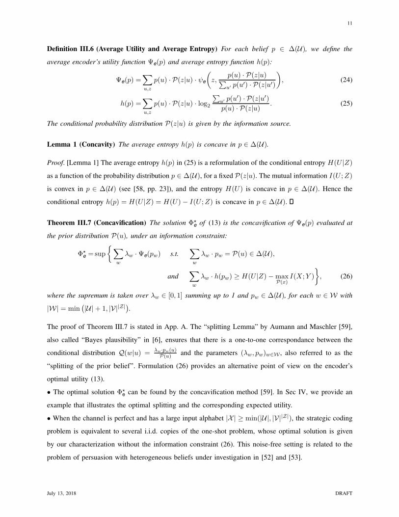
Definition III.6 (Average Utility and Average Entropy) For each belief p ∈ ∆(U), we define the
average encoder’s utility function Ψe(p) and average entropy function h(p):
Ψe(p) =∑
u,z
p(u) · P(z|u) · ψe
(z,
p(u) · P(z|u)∑u′ p(u′) · P(z|u′)
), (24)
h(p) =∑
u,z
p(u) · P(z|u) · log2
∑u′ p(u′) · P(z|u′)
p(u) · P(z|u). (25)
The conditional probability distribution P(z|u) is given by the information source.
Lemma 1 (Concavity) The average entropy h(p) is concave in p ∈ ∆(U).
Proof. [Lemma 1] The average entropy h(p) in (25) is a reformulation of the conditional entropy H(U |Z)
as a function of the probability distribution p ∈ ∆(U), for a fixed P(z|u). The mutual information I(U ;Z)
is convex in p ∈ ∆(U) (see [58, pp. 23]), and the entropy H(U) is concave in p ∈ ∆(U). Hence the
conditional entropy h(p) = H(U |Z) = H(U)− I(U ;Z) is concave in p ∈ ∆(U).
Theorem III.7 (Concavification) The solution Φ⋆e of (13) is the concavification of Ψe(p) evaluated at
the prior distribution P(u), under an information constraint:
Φ⋆e =sup
{∑
w
λw ·Ψe(pw) s.t.∑
w
λw · pw = P(u) ∈ ∆(U),
and∑
w
λw · h(pw) ≥ H(U |Z)−maxP(x)
I(X;Y )
}, (26)
where the supremum is taken over λw ∈ [0, 1] summing up to 1 and pw ∈ ∆(U), for each w ∈ W with
|W| = min(|U|+ 1, |V||Z|
).
The proof of Theorem III.7 is stated in App. A. The “splitting Lemma” by Aumann and Maschler [59],
also called “Bayes plausibility” in [6], ensures that there is a one-to-one correspondance between the
conditional distribution Q(w|u) = λw ·pw(u)P(u) and the parameters (λw, pw)w∈W , also referred to as the
“splitting of the prior belief”. Formulation (26) provides an alternative point of view on the encoder’s
optimal utility (13).
• The optimal solution Φ⋆e can be found by the concavification method [59]. In Sec IV, we provide an
example that illustrates the optimal splitting and the corresponding expected utility.
• When the channel is perfect and has a large input alphabet |X | ≥ min(|U|, |V||Z|), the strategic coding
problem is equivalent to several i.i.d. copies of the one-shot problem, whose optimal solution is given
by our characterization without the information constraint (26). This noise-free setting is related to the
problem of persuasion with heterogeneous beliefs under investigation in [52] and [53].
July 13, 2018 DRAFT

12
• The information constraint∑
w λw · h(pw) ≥ H(U |Z) −maxP(x) I(X;Y ) in (26) is a reformulation
of I(U ;W |Z) ≤ maxP(x) I(X;Y ) in (11):
∑
w
λw · h(pw) =∑
w
λw ·H(U |Z,W = w) (27)
=H(U |Z,W ). (28)
• The dimension of the problem (26) is |U|. Caratheodory’s Lemma (see [60, Corollary 17.1.5, pp. 157]
and [49, Corollary A.4, pp. 39]) provides the cardinality bound: |W| = |U|+ 1.
• The cardinality of W is also restricted to the vector of recommended actions |W| = |V||Z|, telling to
the decoder which action to play in each state. Otherwise assume that two posteriors pw1and pw2
induce
the same vectors of actions v1 = (v11 , . . . , v1|Z|) = v2 = (v21 , . . . , v
2|Z|). Then, both posteriors pw1
and pw2
can be replaced by their average:
p =λw1
· pw1+ λw2
· pw2
λw1+ λw2
, (29)
without changing the utility and still satisfying the information constraint:
h(p) ≥λw1
· h(pw1) + λw2
· h(pw2)
λw1+ λw2
(30)
=⇒∑
w 6=w1,
w 6=w2
λw · h(pw) + (λw1+ λw2
) · h(p) ≥ H(U |Z)−maxP(x)
I(X;Y ). (31)
Inequality (30) comes from the concavity of h(p), stated in Lemma 1.
Following the arguments of [49, Theorem 5.1], the splitting under information constraint of Theorem
III.7 can be reformulated in terms of Lagrangian and in terms of a general concavification Ψe(p, ν)
defined by:
Ψe(p, ν) =
Ψe(p), if ν ≤ h(p),
−∞, otherwise,(32)
Theorem III.8 The optimal solution Φ⋆e reformulates as:
Φ⋆e = inf
t≥0
{cav
[Ψe + t · h
](P(u)
)− t ·
(H(U |Z)−max
P(x)I(X;Y )
)}(33)
=cav Ψe
(P(u),H(U |Z) −max
P(x)I(X;Y )
). (34)
Equation (33) is the concavification of a Lagrangian that integrates the information constraint. The proof
follows directly from [49, Proposition A.2, pp. 37].
Equation (34) corresponds to a bi-variate concavification where the information constraint requires an
additional dimension. The proof follows directly from [49, Lemma A.1, pp. 36].
July 13, 2018 DRAFT

13
IV. EXAMPLE WITH BINARY SOURCE AND STATE
We consider a binary source U ∈ {u1, u2} with probability P(u2) = p0 ∈ [0, 1]. The binary state
information Z ∈ {z1, z2} is drawn according to the conditional probability distribution P(z|u) with
parameter δ1 ∈ [0, 1] and δ2 ∈ [0, 1], as depicted in Fig. 2. For the clarity of the presentation, we
consider a binary auxiliary random variable W ∈ {w1, w2}, even if this choice might be sub-optimal
since: |W| = min(|U| + 1, |V||Z|
)= 3. The solutions provided below implicitly refer to this special
case of |W| = 2. The random variable W is drawn according to the conditional probability distribution
Q(w|u) with parameters α ∈ [0, 1] and β ∈ [0, 1]. The joint probability distribution P(u, z) × Q(w|u)
is represented by Fig. 2. The utility functions of the encoder φe(u, v) and decoder φd(u, v) are given by
u2
u1
b
b
b
b
b
b
b
b
w2
w1
z2
z11− α
1− β
1− p0
p0
α
β
1− δ1
δ1
1− δ2
δ2
Fig. 2. Joint probability distribution P(u, z)×Q(w|u) depending on parameters p0 ∈ [0, 1], δ1 ∈ [0, 1], δ2 ∈ [0, 1], α ∈ [0, 1]
and β ∈ [0, 1].
Fig. 3, 4 and do not depend on the state z. In this example, the goal of the decoder is to choose the
action v that matches the source symbol u, whereas the goal of encoder is to persuade the decoder to
take the action v2. After receiving the pair of symbols (w, z), the decoder updates its posterior belief
u2
u1
v1 v2
0
0
1
1
Fig. 3. Utility function of the encoder φe(u, v).
u2
u1
v1 v2
9
4
0
10
Fig. 4. Utility function of the decoder φd(u, v).
P(·|w, z) ∈ ∆(U), according to Bayes rule. We denote by p ∈ ∆(U) the decoder’s belief and we denote
by γ = 0.6 the belief threshold at which the decoder changes its action. When the decoder’s belief
is exactly equal to the threshold p(u2) = γ = 0.6, the decoder is indifferent between the two actions
{v1, v2} so it chooses v1, i.e. the worst action for the encoder. Hence the decoder chooses a best-reply
action v⋆1 or v⋆2 depending on the interval [0, 0.6] or ]0.6, 1] in which lies the belief p(u2) ∈ [0, 1], see
Fig. 5. Since the utility functions given by Fig. 3, 4 do not depends on Z , we denote by ψe(p) the robust
July 13, 2018 DRAFT

14
0 1 p(u2)D
ecod
er’s
Exp
ecte
dU
tility
v⋆19
4
v⋆2 10
b
0.6
Fig. 5. The decoder’s best-reply action v⋆ depends on its belief p ∈ ∆(U): it plays v⋆1 if p(u2) ∈ [0, 0.6] and v⋆2 if p(u2) ∈
]0.6, 1].
utility function of the encoder (see Definition III.5), given by:
ψe(p) = minv∈argmax
p(u1)·φd(u1,v)+p(u2)·φ
d(u2,v)
p(u1) · φe(u1, v) + p(u2) · φe(u2, v), (35)
= 1
(p(u2) ∈]0.6, 1]
). (36)
A. Concavification without Information Constraint
In this section, we assume that the channel capacity is large enough maxP(x) I(X;Y ) ≥ log2 |U|, so
we investigate the concavification of Ψe(p) (see Definition III.6), without information constraint:
Φ◦e =sup
{∑
w
λw ·Ψe(pw) s.t.∑
w
λw · pw = P(u) ∈ ∆(U)
}. (37)
The correlation between random variables (U,Z) is fixed whereas the correlation between random
variables (U,W ) is chosen strategically by the encoder. This imposes a strong relationship between
the three different kinds of posterior beliefs: Q(u|z), Q(u|w), Q(u|w, z). We denote by p01 ∈ [0, 1],
p02 ∈ [0, 1] the belief parameters after observing the state information Z only:
p01 = Q(u2|z1) =p0 · δ2
p0 · δ2 + (1− p0) · (1− δ1), (38)
p02 = Q(u2|z2) =p0 · (1− δ2)
p0 · (1− δ2) + (1− p0) · δ1. (39)
The beliefs parameters p01, p02 are given by the source probability distribution P(u, z) ∈ ∆(U × Z)
and correspond to the horizontal dotted lines in Fig. 8, for p0 = 0.5, δ1 = 0.7, δ2 = 0.9. We denote by
July 13, 2018 DRAFT

15
q1 ∈ [0, 1], q2 ∈ [0, 1] the belief parameters after observing only the symbol W sent by the encoder:
q1 = Q(u2|w1) =p0 · β
p0 · β + (1− p0) · (1− α), (40)
q2 = Q(u2|w2) =p0 · (1− β)
p0 · (1− β) + (1− p0) · α. (41)
By inverting the system of equations (40) - (41), we express the cross-over probabilities α(q1, q2) and
β(q1, q2) as functions of the target belief parameters (q1, q2):α(q1, q2) = (1−q2)·(q1−p0)
(1−p0)·(q1−q2)
β(q1, q2) = q1·(p0−q2)p0·(q1−q2)
(42)
Lemma 2 (Feasible Posteriors) The parameters α(q1, q2) and β(q1, q2) belong to the interval [0, 1] if
and only if q1 ≤ p0 ≤ q2 or q2 ≤ p0 ≤ q1.
The proof of Lemma 2 is stated in App. D. Thanks to the Markov chain property Z −− U −−W the
posterior beliefs Q(u|w, z) reformulate in terms of Q(u|w):
Q(u|w, z) =Q(u, z, w)
Q(z, w)=
Q(u, z|w)∑u′ Q(u′, z|w)
=Q(u|w)P(z|u)∑u′ Q(u′|w)P(z|u′)
, ∀(u, z, w) ∈ U × Z ×W.
(43)
0
1
1p0 =
0.5
p0 = 0.5
p01 = 0.750000
p02 = 0.125000
p1
γ = 0.6
ν1 =
0.333333
ν2 =
0.913043
b b
b b
q1 q2
b
b
b
b p3(ν2) = 0.969231
p2(ν1) = 0.066667
p1
p2
p3
p4
Fig. 6. Posterior beliefs (p1, p2) depending on q1 ∈ [0, p0] and posterior beliefs (p3, p4) depending on q2 ∈ [p0, 1], for p0 = 0.5,
δ1 = 0.7, δ2 = 0.9 and γ = 0.6.
July 13, 2018 DRAFT

16
We define the belief parameters p1 ∈ [0, 1], p2 ∈ [0, 1], p3 ∈ [0, 1], p4 ∈ [0, 1] after observing (W,Z)
and we express them as functions of q1, q2:
p1 = Q(u2|w1, z1) =q1 · δ2
(1− q1) · (1− δ1) + q1 · δ2, (44)
p2 = Q(u2|w1, z2) =q1 · (1− δ2)
(1− q1) · δ1 + q1 · (1− δ2), (45)
p3 = Q(u2|w2, z1) =q2 · δ2
(1− q2) · (1− δ1) + q2 · δ2, (46)
p4 = Q(u2|w2, z2) =q2 · (1− δ2)
(1− q2) · δ1 + q2 · (1− δ2). (47)
Fig. 6 represents (p1, p2, p3, p4) as a functions of q1 ∈ [0, p0] and q2 ∈ [p0, 1]. In fact, the beliefs q1 and
q2, are the key parameters since they control the decoder’s best-reply action v⋆(p) through the beliefs
(p1, p2, p3, p4). We define the two following functions of q ∈ [0, 1]:
p1(q) =q · δ2
(1− q) · (1− δ1) + q · δ2, (48)
p2(q) =q · (1− δ2)
(1− q) · δ1 + q · (1− δ2). (49)
Given the belief threshold γ = 0.6 at which the decoder changes its action, we define the parameters ν1
and ν2 such that p1(ν1) = γ and p2(ν2) = γ.
γ = p1(ν1) ⇐⇒ ν1 =γ · (1− δ1)
δ2 · (1− γ) + γ · (1− δ1), (50)
γ = p2(ν2) ⇐⇒ ν2 =γ · δ1
γ · δ1 + (1− δ2) · (1− γ). (51)
This belief parameters ν1 and ν2 allow to reformulate the utility function of the encoder as a function
of belief Q(u|w) (see Fig. 7), instead of belief Q(u|w, z) (see Fig. 8).
The solution Φ◦e corresponds to the concavification of the function Ψe, defined over q ∈ [0, 1]:
Ψe(q) =((1− q) · (1− δ1) + q · δ2
)· ψe
(p1(q)
)+((1− q) · δ1 + q · (1− δ2)
)· ψe
(p2(q)
), (52)
Φ◦e = cavΨe(p0) = sup
λ,
q,q′
{λ ·Ψe(q) + (1− λ) ·Ψe(q
′) s.t. λ · q + (1− λ) · q′ = p0
}. (53)
Fig. 7 represents the utility function Ψe(q) of the encoder, depending on the belief q ∈ [0, 1]. When
the belief q ∈ [ν1, ν2], then ψe
(p1(q)
)= 1 whereas ψe
(p2(q)
)= 0. The optimal splitting is represented
by the square and circle. This indicates that the optimal posterior beliefs are (p1, p2) = (γ, p2(ν1)) and
(p3, p4) = (p1(ν2), γ), as in Fig. 8.
When the decoder has no state information, the optimal solution by Kamenica-Gentzkow [6] is the
concavification of the function ψe(p) = 1(p ∈]0.6, 1]
), corresponding to Φe in Fig. 8. In this example,
the decoder’s state information Z decreases the optimal utility of the encoder Φe ≥ Φ◦e.
July 13, 2018 DRAFT

17
0
1
1qp
0 =0.5
ν1 =
0.333333
ν2 =
0.913043
b bb
b
b
b
b b Φ◦e = 0.643750
r
b(v⋆1, v⋆1)
(v⋆2, v⋆2)
(v⋆2, v⋆1)
Fig. 7. Optimal encoder’s utility depending on the belief parameter q ∈ [0, 1] after observing W , for parameters p0 = 0.5,
δ1 = 0.7, δ2 = 0.9 and γ = 0.6.
B. Concavification with Information constraint
In this section, we assume that the channel capacity is equal to: C = maxP(x) I(X;Y ) = 0.1, so the
information constraint of Q0 is active. The average entropy stated in (25) reformulates as a function of
q ∈ [0, 1]:
h(q) =((1− q) · (1− δ1) + q · δ2
)·Hb
(p1(q)
)+((1− q) · δ1 + q · (1− δ2)
)·Hb
(p2(q)
), (54)
where Hb(·) denotes the binary entropy. The dark blue region in Fig. 9 represents the set of posterior
distributions (q1, q2) with q1 ≤ p0 ≤ q2 or q2 ≤ p0 ≤ q1, that satisfy the information constraint:
p0 − q2q1 − q2
· h(q1) +q1 − p0q1 − q2
· h(q2) ≥ H(U |Z)−maxP(x)
I(X;Y ) (55)
⇐⇒Q(w1) ·H(U |Z,W = w1) +Q(w2) ·H(U |Z,W = w2) ≥ H(U |Z)−maxP(x)
I(X;Y ) (56)
⇐⇒I(U ;W |Z) ≤ maxP(x)
I(X;Y ). (57)
The green region in Fig. 9 corresponds to the information constraint I(U ;W ) ≤ maxP(x) I(X;Y ), i.e.
when the decoder does not observe the state information Z . The case without decoder’s state information
July 13, 2018 DRAFT

18
0
1
1p(u2)
p 0=0.5
b
b Φe = 0.833333
v⋆1v⋆2
p 01=0.750000
b
b
b
br
p 02=0.125000
p2 =
p2 (ν
1 ) =0.066667
p3 =
p1 (ν
2 ) =0.969231
p1 =
p4 =
γ=0.6
b
r b
b
b b Φ◦e = 0.643750
Fig. 8. Optimal encoder’s utility depending on the belief p(u2) ∈ [0, 1] after observing (W,Z), for parameters p0 = 0.5,
δ1 = 0.7, δ2 = 0.9 and γ = 0.6.
Z is investigated in [49] and the corresponding information constraint is given by:
p0 − q2q1 − q2
·Hb(q1) +q1 − p0q1 − q2
·Hb(q2) ≥ H(U)−maxP(x)
I(X;Y ) (58)
⇐⇒Q(w1) ·H(U |W = w1) +Q(w2) ·H(U |W = w2) ≥ H(U)−maxP(x)
I(X;Y ) (59)
⇐⇒I(U ;W ) ≤ maxP(x)
I(X;Y ). (60)
Fig. 9 shows that the decoder’s state information Z enlarges the set of posterior beliefs Q(u|w) compatible
with the information constraint of Q0.
The optimal posterior beliefs are represented on Fig. 10, by the square and the circle. Due to the
restriction imposed by the channel, the optimal posterior beliefs are (ν3, ν2) instead of (ν1, ν2), and this
reduces the encoder’s optimal utility to Φ⋆e ≃ 0.63 instead of Φ◦
e ≃ 0.64. In fact, the posterior beliefs
(ν1, ν2) do not satisfy the information constraint: λh(ν1)+ (1−λ)h(ν2) < H(U |Z)−maxP(x) I(X;Y ),
whereas the pair of posterior beliefs (ν3, ν2) lies at the boundary of the blue region in Fig. 9. Posterior
beliefs (ν3, ν2) determine the posterior beliefs (p1, p2, p3, p4), represented in Fig. 11, that satisfy the
July 13, 2018 DRAFT

19
p0 =
0.5
p0 = 0.5
0
1
q2
1 q1b
b
b
ν3 =
0.383
ν2 = 0.913
Fig. 9. Regions of posterior beliefs (q1, q2) satisfying the information constraints: I(U ;W |Z) ≤ C in dark blue, and I(U ;W ) ≤
C in green, for p0 = 0.5, δ1 = 0.7, δ2 = 0.9 and channel capacity C = 0.1.
0
1
1qp
0 =0.5
ν1 =
0.333333
ν2 =
0.913043
b b
b
b
b
b
rb b Φ⋆
e = 0.6337
ν3 =
0.383
(v⋆1, v⋆1)
(v⋆2, v⋆2)
(v⋆2, v⋆1)
bbH(U |Z)− C
b
b
b
bb
Fig. 10. Optimal encoder’s utility depending on the belief parameter q ∈ [0, 1] after observing W , for parameters p0 = 0.5,
δ1 = 0.7, δ2 = 0.9, γ = 0.6 and C = 0.1. The curve represents the average entropy h(q) = H(U |Z) defined in (54), as a
function of q ∈ [0, 1].
July 13, 2018 DRAFT

20
0
1
1p(u2)
p 0=0.5
bbH(U |Z)− C
b
v⋆1v⋆2
p 01=0.750000
b
b
bb
brb
b
b
p 02=0.125000
p2 =
p2 (ν
1 ) =0.0815
p3 =
p1 (ν
2 ) =0.969231
p4 =
γ=0.6
p1 =
0.6506
b
br
b
b
b
b
b
b b Φ⋆e = 0.6337
Fig. 11. Optimal encoder’s utility depending on the belief p(u2) ∈ [0, 1] after observing (W,Z), for parameters p0 = 0.5,
δ1 = 0.7, δ2 = 0.9 and γ = 0.6. The curve represents the binary entropy Hb(·), as a function of p(u2) ∈ [0, 1].
reformulation of the information constraint:
λw1,z1Hb(p1) + λw1,z2Hb(p2) + λw2,z1Hb(p3) + λw2,z2Hb(p4) = H(U |Z)−maxP(x)
I(X;Y ), (61)
and provide the corresponding expected utility Φ⋆e ≃ 0.63.
Remark IV.1 (Impact of the State Information Z) The state information Z at the decoder has two
effects:
• When the communication is restricted (i.e. maxP(x) I(X;Y ) < log2 |U|), it enlarges the set of posterior
beliefs Q(u|w), so it may increase the encoder’s utility.
• Since it reveals partial information to the decoder, it forces the decoder to choose a best-reply actions
that might be sub-optimal for the encoder, so it may decrease the encoder’s utility.
Depending on the problem, the state information Z may increase or decrease the encoder’s optimal utility.
July 13, 2018 DRAFT

21
APPENDIX A
PROOF OF THEOREM III.7
We identify the weight parameters λw = Q(w) and pw = Q(u|w) ∈ ∆(U) and (26) becomes:
supλw∈[0,1],
pw∈∆(U)
{∑
w
λw ·Ψe(pw) s.t.∑
w
λw · pw = P(u) ∈ ∆(U),
and∑
w
λw · h(pw) ≥ H(U |Z)−maxP(x)
I(X;Y )
}(62)
= supQ(w),Q(u|w)
{∑
w
Q(w) ·Ψe(Q(u|w)) s.t.∑
w
Q(w) · Q(u|w) = P(u) ∈ ∆(U),
and∑
w
Q(w) · h(Q(u|w)) ≥ H(U |Z)−maxP(x)
I(X;Y )
}(63)
= supQ(w),Q(u|w)
{∑
w
Q(w) ·∑
u,z
Q(u|w) · P(z|u) · ψe
(z,Q(u|w, z)
),
s.t.∑
w
Q(w) · Q(u|w) = P(u) ∈ ∆(U),
and∑
w
Q(w) ·∑
u,z
Q(u|w) · P(z|u) · log21
Q(u|w, z)≥ H(U |Z)−max
P(x)I(X;Y )
}(64)
= supQ(w),Q(u|w)
{∑
w
Q(w) ·∑
u,z
Q(u|w) · P(z|u) · ψe
(z,Q(u|w, z)
),
s.t.∑
w
Q(w) · Q(u|w) = P(u) ∈ ∆(U), and H(U |W,Z) ≥ H(U |Z)−maxP(x)
I(X;Y )
}(65)
= supQ(u,z,w)∈Q0
EQ(u,z,w)
[φe(U,Z, V
⋆(z,Q(u|w, z)))
](66)
= supQ(u,z,w)∈Q0
minQ(v|z,w)∈
Q2(Q(u,z,w))
E Q(u,z,w)
×Q(v|z,w)
[φe(U,Z, V )
]= Φ⋆
e. (67)
Equation (63) comes from the identification of the weight parameters λw = Q(w) and pw = Q(u|w) ∈
∆(U).
Equation (64) comes from the definitions of Ψe(pw) and h(pw) in (24) and (25) and from: Q(u|w, z) =
Q(u,z|w)Q(z|w) = Q(u|w)·P(z|u)∑
u′ Q(u′|w)·P(z|u′) , due to the Markov chain property Z−−U −−W and the fixed distribution
of the source P(u, z).
Equations (65) - (67) are reformulations.
APPENDIX B
ACHIEVABILITY PROOF OF THEOREM III.3
This proof is built on Wyner-Ziv’s source coding [48] and the achievability proof stated in [49, App.
A.3.2, pp. 44] with one additional feature: we show that the average posterior beliefs induced by Wyner-
July 13, 2018 DRAFT

22
Ziv’s source coding converge to the target posterior beliefs.
A. Zero Capacity
We first investigate the case of zero capacity.
Lemma 3 If the channel has zero capacity: maxP(x) I(X;Y ) = 0, then we have:
∀n ∈ N, ∀σ, minτ∈BRd(σ)
Φne (σ, τ) = Φ⋆
e. (68)
Proof. [Lemma 3] The zero capacity maxP(x) I(X;Y ) = 0 implies that any probability distribution
P(u, z)×Q(w|u) ∈ Q0 satisfies I(U ;W |Z) = 0, corresponding to the Markov chain property U−−Z−−W ,
i.e. Q(u|z, w) = P(u|z) for all (u, z, w) ∈ U ×Z ×W .
Φ⋆e = sup
Q(u,z,w)∈Q0
minQ(v|z,w)∈
Q2(Q(u,z,w))
E Q(u,z,w)
×Q(v|z,w)
[φe(U,Z, V )
](69)
= supQ(u,z,w)∈Q0
EQ(u,z,w)
[φe(U,Z, V
⋆(z,Q(u|w, z)))
](70)
= supQ(u,z,w)∈Q0
EQ(u,z,w)
[φe(U,Z, V
⋆(z,P(u|z)))
](71)
=EP(u,z)
[φe(U,Z, V
⋆(z,P(u|z)))
]. (72)
Equation (70) is a reformulation by using the best-reply action v⋆(z, p)
of Definition III.4 for symbol
z ∈ Z and the belief Q(u|w, z).
Equation (71) comes from Markov chain property U−−Z−−W that allows to replace the belief Q(u|w, z)
by P(u|z).
Equation (72) comes from removing the random variable W since it has no impact on the function
φe(u, z, v⋆(z,P(u|z))).
For any n and for any encoding strategy σ, the encoder’s long-run utility is given by:
minτ∈BRd(σ)
Φne (σ, τ) = min
τ∈BRd(σ)
∑
un,zn,xn,
yn,vn
n∏
i=1
P(ui, zi
)× σ
(xn∣∣un)×
n∏
i=1
T(yi)× τ(vn∣∣yn, zn
)·
[1
n
n∑
i=1
φe(ui, zi, vi)
]
(73)
= minτ∈BRd(σ)
∑
un,zn,vn
n∏
i=1
P(ui, zi
)× τ(vn∣∣zn)·
[1
n
n∑
i=1
φe(ui, zi, vi)
](74)
=1
n
n∑
i=1
[ ∑
ui,zi,vi
P(ui, zi
)× 1(v⋆i (zi,Q(u|z))) · φe(ui, zi, vi)
](75)
= EP(u,z)
[φe(U,Z, V
⋆(z,P(u|z)))
]. (76)
July 13, 2018 DRAFT

23
Equation (73) comes from the zero capacity that imposes that the channel outputs Y n are independent
of the channel inputs Xn.
Equation (74) comes from removing the random variables (Xn, Y n) and noting that the decoder’s best-
reply τ(vn∣∣zn)
does not depend on yn anymore, since yn is independent of (un, zn).
Equation (75) is a reformulation based on the best-reply action v⋆(z,P(u|z)
)of Definition III.4, for the
symbol z ∈ Z and the belief P(u|z).
Equation (76) comes from the i.i.d. property of (U,Z) and concludes the proof of Lemma 3.
B. Positive Capacity
We now assume that the channel capacity is strictly positive maxP(x) I(X;Y ) > 0. We consider an
auxiliary concavification in which the information constraint is satisfied with strict inequality and the
sets of decoder’s best-reply actions are always singletons.
Φe =sup
{∑
w
λw ·Ψe(pw) s.t.∑
w
λw · pw = P(u) ∈ ∆(U),
and∑
w
λw · h(pw) > H(U |Z)−maxP(x)
I(X;Y ),
and ∀(z, w) ∈ Z ×W, V⋆(z,Q(u|z, w)) is a singleton
}, (77)
Lemma 4 If maxP(x) I(X;Y ) > 0, then Φe = Φ⋆e.
For the proof of Lemma 4, we refers directly to the similar proof of [49, Lemma A.7, pp. 46]. We denote
by Qn(u, z, w) the empirical distribution of the sequence (un, zn, wn) and we denote by Aδ the set of
typical sequences with tolerance δ > 0, defined by:
Aδ =
{(un, zn, wn, xn, yn), s.t. ||Qn(u, z, w) − P(u, z) ×Q(w|u)||1 ≤ δ,
and ||Qn(x, y)− P⋆(x)× T (y|x)||1 ≤ δ
}. (78)
We define Tα(wn, yn, zn) and Bα,γ,δ depending on parameters α > 0 and γ > 0:
Tα(wn, yn, zn) =
{i ∈ {1, . . . , n}, s.t. D
(Pσ(Ui|y
n, zn)∣∣∣∣∣∣Q(Ui|wi, zi)
)≤
α2
2 ln 2
}, (79)
Bα,γ,δ =
{(wn, yn, zn), s.t.
|Tα(wn, yn, zn)|
n≥ 1− γ and (wn, yn, zn) ∈ Aδ
}. (80)
The notation Bcα,γ,δ stands for the complementary set of Bα,γ,δ ⊂ Wn × Yn × Zn. The sequences
(wn, yn, zn) belong to the set Bα,γ,δ if: 1) they are typical and 2) if the corresponding posterior belief
Pσ(Ui|yn, zn) is close in K-L divergence to the target belief Q(Ui|wi, zi), for a large fraction of stages
i ∈ {1, . . . , n}.
July 13, 2018 DRAFT

24
The cornerstone of this achievability proof is Proposition B.1, which refines the analysis of Wyner-Ziv’s
source coding, by characterizing its posterior beliefs.
Proposition B.1 (Wyner-Ziv’s Posterior Beliefs) If the probability distribution P(u, z) ×Q(w|u) sat-
isfies:
maxP(x) I(X;Y )− I(U ;W |Z) > 0,
V⋆(z,Q(u|z, w)) is a singleton ∀(z, w) ∈ Z ×W,
(81)
then
∀ε > 0, ∀α > 0, ∀γ > 0, ∃δ > 0, ∀δ < δ, ∃n ∈ N⋆, ∀n ≥ n,∃σ, s.t. Pσ(Bcα,γ,δ) ≤ ε. (82)
The proof of proposition B.1 is stated in App. B-C.
Proposition B.2 For any encoding strategy σ, we have:∣∣∣∣ minτ∈BRd(σ)
Φne (σ, τ)− Φe
∣∣∣∣ ≤ (α+ 2γ + δ) · φe + (1− Pσ(Bα,γ,δ)) · φe, (83)
where φe = maxu,z,v φe(u, z, v) is the largest absolute value of encoder’s utility.
For the proof of Proposition B.2, we refers directly to the similar proof of [49, Corollary A.18, pp. 53].
Corollary B.3 For any ε > 0, there exists n ∈ N⋆ such that for all n ≥ n there exists an encoding
strategy σ such that:∣∣∣∣ minτ∈BRd(σ)
Φne(σ, τ) − Φe
∣∣∣∣ ≤ ε. (84)
The proof of Corollary B.3 comes from combining Proposition B.1 with Proposition B.2 and choosing
parameters α, γ, δ small and n ∈ N⋆ large. This concludes the achievability proof of Theorem III.3.
C. Proof of Proposition B.1
We assume that the probability distribution P(u, z) ×Q(w|u) satisfies the two following conditions:
maxP(x) I(X;Y )− I(U ;W |Z) > 0,
V⋆(z,Q(u|z, w)) is a singleton ∀(z, w) ∈ Z ×W,
(85)
The strict information constraint ensures there exists a small parameter η > 0 and rates R ≥ 0, RL ≥ 0,
such that:
R + RL = I(U ;W ) + η, (86)
RL ≤ I(Z;W )− η, (87)
R ≤ maxP(x)
I(X;Y )− η. (88)
July 13, 2018 DRAFT

25
We now recall the random coding construction of Wyner-Ziv [48] and we investigate the corresponding
posterior beliefs. We note by Σ the random encoding/decoding, defined as follows:
• Random codebook. We defines the indices m ∈ M with |M| = 2nR and l ∈ ML with |ML| = 2nRL .
We draw |M×ML| = 2n(R+RL) sequences W n(m, l) with the i.i.d. probability distribution Q⊗n(w),
and |M| = 2nR sequences Xn(m), with the i.i.d. probability distribution P⊗n(x) that maximizes
the channel capacity in (88).
• Encoding function. The encoder observes the sequence of symbols of source Un ∈ Un and finds a
pair of indices (m, l) ∈ M×ML such that the sequences(Un,W n(m, l)
)∈ Aδ are jointly typical.
It sends the sequence Xn(m) corresponding to the index m ∈ M.
• Decoding function. The decoder observes the sequence of channel output Y n ∈ Yn. It returns an
index m ∈ M such that the sequences(Y n,Xn(m)
)∈ Aδ are jointly typical. Then it observes
the sequence of state information Zn ∈ Zn and returns an index l ∈ ML such that the sequences(Zn,W n(m, l)
)∈ Aδ are jointly typical.
• Error Event. We introduce the event of error Eδ ∈ {0, 1} defined as follows:
Eδ =
{0 if (M,L) = (M , L) and
(Un, Zn,W n,Xn, Y n
)∈ Aδ,
1 otherwise.(89)
Expected error probability of the random encoding/decoding Σ. For all ε2 > 0, for all η > 0, there
exists a δ > 0, for all δ ≤ δ there exists n such that for all n ≥ n, the expected probability of the
following error events are bounded by ε2:
EΣ
[P
(∀(m, l),
(Un,W n(m, l)
)/∈ Aδ
)]≤ ε2, (90)
EΣ
[P
(∃l′ 6= l, s.t.
(Zn,W n(m, l′)
)∈ Aδ
)]≤ ε2, (91)
EΣ
[P
(∃m′ 6= m, s.t.
(Y n,Xn(m′)
)∈ Aδ
)]≤ ε2, (92)
Eq. (90) comes from (86) and the covering lemma [58, pp. 208].
Eq. (91) comes from (87) and the packing lemma [58, pp. 46].
Eq. (92) comes from (88) and the packing lemma [58, pp. 46].
There exists a coding strategy σ with small error probability:
∀ε2 > 0, ∀η > 0, ∃δ > 0, ∀δ ≤ δ, ∃n > 0, ∀n ≥ n, ∃σ, Pσ
(Eδ = 1
)≤ ε2. (93)
July 13, 2018 DRAFT

26
Control of the posterior beliefs. We assume that the event Eδ = 0 is realized and we investigate the
posterior beliefs Pσ(ui|yn, zn, Eδ = 0) induced by Wyner-Ziv’s encoding strategy σ.
Eσ
[1
n
n∑
i=1
D
(Pσ(Ui|Y
n, Zn, Eδ = 0)
∣∣∣∣∣∣∣∣Q(Ui|Wi, Zi)
)]
=∑
(wn,zn,yn)∈Aδ
Pσ(wn, zn, yn|Eδ = 0)×
1
n
n∑
i=1
D
(Pσ(Ui|y
n, zn, Eδ = 0)
∣∣∣∣∣∣∣∣Q(Ui|wi, zi)
)(94)
=1
n
∑
(un,zn,wn,yn)∈Aδ
Pσ(un, zn, wn, yn|Eδ = 0)× log2
1∏ni=1Q(ui|wi, zi)
−1
n
n∑
i=1
H(Ui|Yn, Zn, Eδ = 0)
(95)
≤H(U |W,Z)−1
nH(Un|W n, Y n, Zn, Eδ = 0) + δ (96)
≤H(U |W,Z)−1
nH(Un|W n, Zn, Eδ = 0) + δ (97)
=H(U |W,Z)−1
nH(Un|Eδ = 0) +
1
nI(Un;W n|Eδ = 0)
+1
nH(Zn|W n, Eδ = 0)−
1
nH(Zn|Un,W n, Eδ = 0) + δ. (98)
Eq. (94)-(95) come from the hypothesis Eδ = 0 of typical sequences (un, zn, wn, yn) ∈ Aδ and the
definition of the conditional K-L divergence [54, pp. 24].
Eq. (96) comes from property of typical sequences [58, pp. 26] and the conditioning that reduces entropy.
Eq. (97) comes from the Markov chain Zn−−Un−−W n−−Y n induced by the strategy σ, that implies
H(Un|W n, Zn, Eδ = 0) = H(Un|W n, Y n, Zn, Eδ = 0).
Eq. (98) is a reformulation of (97).
1
nH(Un|Eδ = 0) ≥ H(U)−
1
n− log2 |U| · Pσ
(Eδ = 1
), (99)
1
nI(Un;W n|Eδ = 0) ≤ R + RL = I(U ;W ) + η, (100)
1
nH(Zn|W n, Eδ = 0) ≤
1
nlog2 |Aδ(z
n|wn)| ≤ H(Z|W ) + δ, (101)
1
nH(Zn|Un,W n, Eδ = 0) ≥ H(Z|U,W )−
1
n− log2 |U| · Pσ
(Eδ = 1
). (102)
Eq. (99) comes from the i.i.d. source and Fano’s inequality.
Eq. (100) comes from the cardinality of codebook given by (86). This argument is also used in [61, Eq.
(23)].
Eq. (101) comes from the cardinality of Aδ(zn|wn), see also [58, pp. 27].
Eq. (102) comes from Fano’s inequality H(Zn|Un,W n), and the Markov chain Zn −− Un −− W n
July 13, 2018 DRAFT

27
H(Zn|Un), the i.i.d. property of the source (U,Z) that implies H(Z|U) and the Markov chain Z−−U−−W
that implies H(Z|U,W ).
Equations (98)-(102) shows that on average, the posterior beliefs Pσ(ui|yn, zn, Eδ = 0) induced by
strategy σ is close to the target probability distribution Q(u|w, z).
Eσ
[1
n
n∑
i=1
D
(Pσ(Ui|Y
n, Zn, Eδ = 0)
∣∣∣∣∣∣∣∣Q(Ui|Wi, Zi)
)]
≤2δ + η +2
n+ 2 log2 |U| · Pσ
(Eδ = 1
):= ǫ. (103)
Then we have:
Pσ(Bcα,γ,δ) =1−Pσ(Bα,γ,δ)
=Pσ(Eδ = 1)Pσ(Bcα,γ,δ|Eδ = 1) + Pσ(Eδ = 0)Pσ(B
cα,γ,δ|Eδ = 0)
≤Pσ(Eδ = 1) + Pσ(Bcα,γ,δ|Eδ = 0)
≤ε2 + Pσ(Bcα,γ,δ|Eδ = 0). (104)
Moreover:
Pσ(Bcα,γ,δ|Eδ = 0)
=∑
wn,yn,zn
Pσ
((wn, yn, zn) ∈ Bc
α,γ,δ
∣∣∣Eδ = 0)
(105)
=∑
wn,yn,zn
Pσ
((wn, yn, zn) s.t.
|Tα(wn, yn, zn)|
n< 1− γ
∣∣∣∣∣Eδ = 0
)(106)
=Pσ
(1
n·
∣∣∣∣{i, s.t. D
(Pσ(Ui|y
n, zn)∣∣∣∣∣∣Q(Ui|wi, zi)
)≤
α2
2 ln 2
}∣∣∣∣ < 1− γ
∣∣∣∣∣Eδ = 0
)(107)
=Pσ
(1
n·
∣∣∣∣{i, s.t. D
(Pσ(Ui|y
n, zn)∣∣∣∣∣∣Q(Ui|wi, zi)
)>
α2
2 ln 2
}∣∣∣∣ ≥ γ
∣∣∣∣∣Eδ = 0
)(108)
≤2 ln 2
α2γ· Eσ
[1
n
n∑
i=1
D(Pσ(Ui|y
n, zn)∣∣∣∣∣∣Q(Ui|wi, zi)
)](109)
≤2 ln 2
α2γ·
(η + δ +
2
n+ 2 log2 |U| · Pσ
(Eδ = 1
)). (110)
Eq. (105) to (108) are simple reformulations.
Eq. (109) comes from the double use of Markov’s inequality as in [49, Lemma A.22, pp.60].
Eq. (110) comes from (103).
Combining equations (93), (104), (110) and choosing η > 0 small, we obtain the following statement:
∀ε > 0, ∀α > 0, ∀γ > 0, ∃δ > 0, ∀δ < δ, ∃n ∈ N⋆, ∀n ≥ n,∃σ, s.t. Pσ(Bcα,γ,δ) ≤ ε. (111)
This concludes the proof of Proposition B.1.
July 13, 2018 DRAFT

28
APPENDIX C
CONVERSE PROOF OF THEOREM III.3
We consider an encoding strategy σ of length n ∈ N. We denote by T the uniform random variable
{1, . . . , n} and the notation Z−T stands for (Z1, . . . , Zt−1, Zt+1, . . . Zn), where ZT has been removed.
We introduce the auxiliary random variable W = (Y n, Z−T , T ) whose joint probability distribution
P(u, z, w) with (U,Z) is defined by:
P(u, z, w) =Pσ
(uT , zT , y
n, z−T , T)
=P(T = i) · Pσ
(uT , zT , y
n, z−T∣∣T = i
)
=1
n· Pσ
(ui, zi, y
n, z−i). (112)
This identification ensures that the Markov chain W −− UT −− ZT is satisfied. Let us fix a decoding
strategy τ(vn|yn, zn) and define τ(v|w, z) = τ (v|yn, z−i, i, z) = τi(vi|yn, zn) where τi denotes the i-th
coordinate of τ(vn|yn, zn). The encoder’s long-run utility writes:
Φne (σ, τ) =
∑
un,zn,yn
Pσ(un, zn, yn)
∑
vn
τ(vn|yn, zn) ·
[1
n
n∑
i=1
φe(ui, zi, vi)
](113)
=
n∑
i=1
∑ui,zi,
z−i,yn
1
n· Pσ(ui, z
n, yn)∑
vi
τi(vi|yn, zn) · φe(ui, zi, vi) (114)
=∑
ui,zi,yn,
z−i,i
Pσ(ui, zi, yn, z−i, i)
∑
vi
τi(vi|zi, yn, z−i, i) · φe(ui, zi, vi) (115)
=∑
u,z,w
P(u, z, w)∑
v
τ(v|w, z) · φe(u, z, v). (116)
Eq. (113) - (115) are reformulations and re-orderings.
Eq. (116) comes from replacing the random variables (Y n, Z−T , T ) by W whose distribution is defined
in (112).
Equations (113) - (116) are also valid for the decoder’s utility Φnd(σ, τ) =
∑u,z,
w,v
P(u, z, w)τ (v|w, z) ·
φd(u, z, v). A best-reply strategy τ ∈ BRd(σ) reformulates as:
τ ∈ argmaxτ ′(vn|yn,zn)
∑
un,zn,
xn,yn,vn
Pσ(un, zn, xn, yn) · τ ′(vn|yn, zn) ·
[1
n
n∑
i=1
φd(ui, zi, vi)
](117)
⇐⇒τ(v|w, z) ∈ argmaxτ ′(v|w,z)
∑
u,z,w
P(u, z, w) · τ ′(v|w, z) · φd(u, z, v) (118)
⇐⇒τ(v|w, z) ∈ Q2
(P(u, z, w)
). (119)
July 13, 2018 DRAFT

29
We now prove that the distribution P(u, z, w) defined in (112), satisfies the information constraint of the
set Q0.
0 ≤I(Xn;Y n)− I(Un, Zn;Y n) (120)
≤n∑
i=1
H(Yi)−n∑
i=1
H(Yi|Xi)− I(Un;Y n|Zn) (121)
≤n ·maxP(x)
I(X;Y )−n∑
i=1
I(Ui;Yn|Zn, U i−1) (122)
=n ·maxP(x)
I(X;Y )−n∑
i=1
I(Ui;Yn, Z−i, U i−1|Zi) (123)
≤n ·maxP(x)
I(X;Y )−n∑
i=1
I(Ui;Yn, Z−i|Zi) (124)
=n ·maxP(x)
I(X;Y )− n · I(UT ;Yn, Z−T |ZT , T ) (125)
=n ·maxP(x)
I(X;Y )− n · I(UT ;Yn, Z−T , T |ZT ) (126)
=n ·maxP(x)
I(X;Y )− n · I(U ;W |Z) (127)
=n ·
(maxP(x)
I(X;Y )− I(U ;W ) + I(Z;W )
). (128)
Eq. (120) comes from the Markov chain Y n −−Xn −− (Un, Zn).
Eq. (121) comes from the memoryless property of the channel and from removing the positive term
I(Un;Zn) ≥ 0.
Eq. (122) comes from taking the maximum P(x) and chain rule.
Eq. (123) comes from the i.i.d. property of the source (U,Z) that implies I(Ui, Zi;Z−i, U i−1) =
I(Ui;Z−i, U i−1|Zi) = 0.
Eq. (124) comes from removing I(Ui;Ui−1|Y n, Z−i, Zi) ≥ 0.
Eq. (125) comes from the uniform random variable T ∈ {1, . . . , n}.
Eq. (126) comes from the independence between T and the source (U,Z), that implies I(UT , ZT ;T ) =
I(UT ;T |ZT ) = 0.
Eq. (127) comes from the identification W = (Y n, Z−T , T ).
Eq. (128) comes from the Markov chain W −−UT −−ZT . This proves that the distribution Pσ(u, z, w)
belongs to the set Q0.
July 13, 2018 DRAFT

30
Therefore, for any encoding strategy σ and all n, we have:
minτ∈BRd(σ)
Φne (σ, τ) (129)
= minτ(v|w,z)∈
Q2(P(u,z,w))
∑
u,z,w
P(u, z, w)∑
v
τ(v|w, z) · φe(u, z, v) (130)
= minτ(v|z,w)∈
Q2(P(u,z,w))
E P(u,z,w)
×τ(v|z,w)
[φe(U,Z, V )
](131)
≤ supQ(u,z,w)∈Q0
minQ(v|z,w)∈
Q2(Q(u,z,w))
E Q(u,z,w)
×Q(v|z,w)
[φe(U,Z, V )
]= Φ⋆
e. (132)
The last inequality comes from the probability distribution P(u, z, w) that satisfies the information
constraint of the set Q0. The first cardinality bound |W| = |U| + 1 comes from [49, Lemma 6.1].
The second cardinality bound for |W| = |V||Z| comes from [49, Lemma 6.3], by considering the encoder
tells to the decoder which action v ∈ V to play in each state z ∈ Z .
This conclude the proof of (20) in Theorem III.3.
APPENDIX D
PROOF OF LEMMA 2
By inverting the system of equations, we have the following equivalence:q1 = p0·β
p0·β+(1−p0)·(1−α)
q2 = p0·(1−β)p0·(1−β)+(1−p0)·α
⇐⇒
α = (1−q2)·(q1−p0)
(1−p0)·(q1−q2)
β = q1·(p0−q2)p0·(q1−q2)
.
(133)
Assume that q1 ≤ q2, then we have:
0 ≤ α⇐⇒ 0 ≤(1− q2) · (q1 − p0)
(1− p0) · (q1 − q2)⇐⇒ q1 − p0 ≤ 0, (134)
α ≤ 1 ⇐⇒(1− q2) · (q1 − p0)
(1− p0) · (q1 − q2)≤ 1 ⇐⇒ q2 − p0 ≥ 0, (135)
0 ≤ β ⇐⇒ 0 ≤q1 · (p0 − q2)
p0 · (q1 − q2)⇐⇒ p0 − q2 ≤ 0, (136)
β ≤ 1 ⇐⇒q1 · (p0 − q2)
p0 · (q1 − q2)≤ 1 ⇐⇒ p0 − q1 ≥ 0. (137)
(138)
This proves the equivalence:
q1 ≤ q2
α ∈ [0, 1]
β ∈ [0, 1]
⇐⇒ q1 ≤ p0 ≤ q2. (139)
July 13, 2018 DRAFT

31
Assume that q1 ≥ q2, then we have:
0 ≤ α⇐⇒ 0 ≤(1− q2) · (q1 − p0)
(1− p0) · (q1 − q2)⇐⇒ q1 − p0 ≥ 0, (140)
α ≤ 1 ⇐⇒(1− q2) · (q1 − p0)
(1− p0) · (q1 − q2)≤ 1 ⇐⇒ q2 − p0 ≤ 0, (141)
0 ≤ β ⇐⇒ 0 ≤q1 · (p0 − q2)
p0 · (q1 − q2)⇐⇒ p0 − q2 ≥ 0, (142)
β ≤ 1 ⇐⇒q1 · (p0 − q2)
p0 · (q1 − q2)≤ 1 ⇐⇒ p0 − q1 ≤ 0. (143)
(144)
This proves the equivalence:
q1 ≥ q2
α ∈ [0, 1]
β ∈ [0, 1]
⇐⇒ q2 ≤ p0 ≤ q1. (145)
Hence there exists probability parameters α ∈ [0, 1] and β ∈ [0, 1] if and only if q1 ≤ p0 ≤ q2 or
q2 ≤ p0 ≤ q1.
REFERENCES
[1] M. Le Treust and T. Tomala, “Information design for strategic coordination of autonomous devices with non-aligned
utilities,” IEEE Proc. of the 54th Annual Allerton Conference on Communication, Control, and Computing, pp. 233–242,
2016.
[2] M. Le Treust and T. Tomala, “Persuasion bayésienne pour la coordination stratégique d’appareils autonomes ayant des
objectifs non-alignés,” in Actes de la Conférence du Groupement de Recherche en Traitement du Signal et des Images
(GRETSI17), Juan-les-Pins, France, 2017.
[3] M. Le Treust and T. Tomala, “Strategic coordination with state information at the decoder,” Proc. of 2018 International
Zurich Seminar on Information and Communication, 2018.
[4] V. P. Crawford and J. Sobel, “Strategic information transmission,” Econometrica, vol. 50, no. 6, pp. 1431–1451, 1982.
[5] F. Forges, “Non-zero-sum repeated games and information transmission,” in: N. Meggido, Essays in Game Theory in Honor
of Michael Maschler, Springer-Verlag, no. 6, pp. 65–95, 1994.
[6] E. Kamenica and M. Gentzkow, “Bayesian persuasion,” American Economic Review, vol. 101, pp. 2590 – 2615, 2011.
[7] H. von Stackelberg, Marketform und Gleichgewicht. Oxford University Press, 1934.
[8] J. Nash, “Non-cooperative games,” Annals of Mathematics, vol. 54, pp. 286–295, 1951.
[9] D. Bergemann and S. Morris, “Information design, Bayesian persuasion, and Bayes correlated equilibrium,” American
Economic Review Papers and Proceedings, vol. 106, pp. 586–591, May 2016.
[10] I. Taneva, “Information design,” Manuscript, School of Economics, The University of Edinburgh, 2016.
[11] D. Bergemann and S. Morris, “Information design: a unified perspective,” Cowles Foundation Discussion Paper No 2075,
2017.
July 13, 2018 DRAFT

32
[12] E. Tsakas and N. Tsakas, “Noisy persuasion,” Working Paper, 2017.
[13] A. Blume, O. J. Board, and K. Kawamura, “Noisy talk,” Theoretical Economics, vol. 2, pp. 395–440, July 2007.
[14] P. Hernández and B. von Stengel, “Nash codes for noisy channels,” Operations Research, vol. 62, pp. 1221–1235, Nov.
2014.
[15] C. Sims, “Implication of rational inattention,” Journal of Monetary Economics, vol. 50, pp. 665–690, April 2003.
[16] M. Gentzkow and E. Kamenica, “Costly persuasion,” American Economic Review, vol. 104, pp. 457 – 462, 2014.
[17] A. Neyman and D. Okada, “Strategic entropy and complexity in repeated games,” Games and Economic Behavior, vol. 29,
no. 1–2, pp. 191–223, 1999.
[18] A. Neyman and D. Okada, “Repeated games with bounded entropy,” Games and Economic Behavior, vol. 30, no. 2,
pp. 228–247, 2000.
[19] A. Neyman and D. Okada, “Growth of strategy sets, entropy, and nonstationary bounded recall,” Games and Economic
Behavior, vol. 66, no. 1, pp. 404–425, 2009.
[20] O. Gossner and N. Vieille, “How to play with a biased coin?,” Games and Economic Behavior, vol. 41, no. 2, pp. 206–226,
2002.
[21] O. Gossner and T. Tomala, “Empirical distributions of beliefs under imperfect observation,” Mathematics of Operation
Research, vol. 31, no. 1, pp. 13–30, 2006.
[22] O. Gossner and T. Tomala, “Secret correlation in repeated games with imperfect monitoring,” Mathematics of Operation
Research, vol. 32, no. 2, pp. 413–424, 2007.
[23] O. Gossner, R. Laraki, and T. Tomala, “Informationally optimal correlation,” Mathematical Programming, vol. 116, no. 1-2,
pp. 147–172, 2009.
[24] O. Gossner, P. Hernández, and A. Neyman, “Optimal use of communication resources,” Econometrica, vol. 74, no. 6,
pp. 1603–1636, 2006.
[25] P. Cuff and L. Zhao, “Coordination using implicit communication,” IEEE Proc. of the Information Theory Workshop (ITW),
pp. 467– 471, 2011.
[26] P. Cuff, H. Permuter, and T. Cover, “Coordination capacity,” IEEE Transactions on Information Theory, vol. 56, no. 9,
pp. 4181–4206, 2010.
[27] P. Cuff and C. Schieler, “Hybrid codes needed for coordination over the point-to-point channel,” in IEEE Proc. of the 49th
Annual Allerton Conference on Communication, Control, and Computing, pp. 235–239, Sept 2011.
[28] M. Le Treust, “Joint empirical coordination of source and channel,” IEEE Transactions on Information Theory, vol. 63,
pp. 5087–5114, Aug 2017.
[29] G. Cervia, L. Luzzi, M. Le Treust, and M. R. Bloch, “Strong coordination of signals and actions over noisy channels with
two-sided state information,” preliminary draft, https://arxiv.org/abs/1801.10543, 2018.
[30] E. Akyol, C. Langbort, and T. Basar, “Information-theoretic approach to strategic communication as a hierarchical game,”
Proceedings of the IEEE, vol. 105, no. 2, pp. 205–218, 2017.
[31] S. Sarıtas, S. Yüksel, and S. Gezici, “Nash and stackelberg equilibria for dynamic cheap talk and signaling games,” in
American Control Conference (ACC), pp. 3644–3649, May 2017.
[32] S. Sarıtas, S. Yüksel, and S. Gezici, “Quadratic multi-dimensional signaling games and affine equilibria,” IEEE Transactions
on Automatic Control, vol. 62, pp. 605–619, Feb 2017.
[33] E. Akyol, C. Langbort, and T. Basar, “Networked estimation-privacy games,” in IEEE Global Conference on Signal and
Information Processing (GlobalSIP), pp. 507–510, Nov 2017.
July 13, 2018 DRAFT

33
[34] F. Farokhi, A. M. H. Teixeira, and C. Langbort, “Estimation with strategic sensors,” IEEE Transactions on Automatic
Control, vol. 62, pp. 724–739, Feb 2017.
[35] J. Y. Y. Jakub Marecek, Robert Shorten, “Signaling and obfuscation for congestion control,” ACM SIGecom Exchanges,
vol. 88, no. 10, pp. 2086–2096, 2015.
[36] S. Dughmi and H. Xu, “Algorithmic bayesian persuasion,” In Proc. of the 47th ACM Symposium on Theory of Computing
(STOC), 2016.
[37] S. Dughmi, “Algorithmic information structure design: A survey,” ACM SIGecom Exchanges, vol. 15, pp. 2–24, Jan 2017.
[38] S. Dughmi, D. Kempe, and R. Qiang, “Persuasion with limited communication,” In Proc. of the 17th ACM conference on
Economics and Computation (ACM EC’17), Maastricht, The Netherlands, 2016.
[39] R. Berry and D. Tse, “Shannon meets Nash on the interference channel,” IEEE Transactions on Information Theory,
vol. 57, pp. 2821– 2836, May 2011.
[40] S. M. Perlaza, R. Tandon, H. V. Poor, and Z. Han, “Perfect output feedback in the two-user decentralized interference
channel,” IEEE Transactions on Information Theory, vol. 61, pp. 5441–5462, Oct 2015.
[41] A. E. Gamal and T. Cover, “Achievable rates for multiple descriptions,” IEEE Transactions on Information Theory, vol. 28,
pp. 851–857, Nov. 1982.
[42] A. Lapidoth, A. Malär, and M. Wigger, “Constrained source-coding with side information,” IEEE Transactions on
Information Theory, vol. 60, pp. 3218–3237, June 2014.
[43] H. Yamamoto, “A rate-distortion problem for a communication system with a secondary decoder to be hindered,” IEEE
Transactions on Information Theory, vol. 34, pp. 835–842, Jul 1988.
[44] H. Yamamoto, “Rate-distortion theory for the Shannon cipher system,” IEEE Transactions on Information Theory, vol. 43,
pp. 827–835, May 1997.
[45] C. Schieler and P. Cuff, “Rate-distortion theory for secrecy systems,” IEEE Transactions on Information Theory, vol. 60,
pp. 7584–7605, Dec 2014.
[46] C. Schieler and P. Cuff, “The henchman problem: Measuring secrecy by the minimum distortion in a list,” IEEE Transactions
on Information Theory, vol. 62, pp. 3436–3450, June 2016.
[47] A. Lapidoth, “On the role of mismatch in rate distortion theory,” IEEE Transactions on Information Theory, vol. 43,
pp. 38–47, Jan 1997.
[48] A. D. Wyner and J. Ziv, “The rate-distortion function for source coding with side information at the decoder,” IEEE
Transactions on Information Theory, vol. 22, pp. 1–11, Jan. 1976.
[49] M. Le Treust and T. Tomala, “Persuasion with limited communication capacity,” preliminary draft,
https://arxiv.org/abs/1711.04474, 2017.
[50] N. Merhav and S. Shamai, “On joint source-channel coding for the Wyner-Ziv source and the Gel’fand-Pinsker channel,”
IEEE Transactions on Information Theory, vol. 49, no. 11, pp. 2844–2855, 2003.
[51] M. Le Treust, “Empirical coordination with two-sided state information and correlated source and state,” in IEEE Proc. of
the International Symposium on Information Theory (ISIT), pp. 466–470, 2015.
[52] “Bayesian persuasion with heterogeneous priors,” Journal of Economic Theory, vol. 165, pp. 672 – 706, 2016.
[53] M. Laclau and L. Renou, “Public persuasion,” working paper, February 2017.
[54] T. M. Cover and J. A. Thomas, Elements of Information Theory. New York: 2nd. Ed., Wiley-Interscience, 2006.
[55] C. E. Shannon, “A mathematical theory of communication,” Bell System Technical Journal, vol. 27, pp. 379–423, 1948.
[56] M. Le Treust and M. Bloch, “Empirical coordination, state masking and state amplification: Core of the decoder’s
knowledge,” IEEE Proc. of the IEEE International Symposium on Information Theory (ISIT), pp. 895–899, 2016.
July 13, 2018 DRAFT

34
[57] M. Le Treust and M. Bloch, “State leakage and coordination of actions: Core of decoder’s knowledge,” preliminary draft,
2018.
[58] A. E. Gamal and Y.-H. Kim, Network Information Theory. Cambridge University Press, Dec. 2011.
[59] R. Aumann and M. Maschler, Repeated Games with Incomplete Information. MIT Press, Cambrige, MA, 1995.
[60] R. Rockafellar, Convex Analysis. Princeton landmarks in mathematics and physics, Princeton University Press, 1970.
[61] N. Merhav and S. Shamai, “Information rates subject to state masking,” IEEE Transactions on Information Theory, vol. 53,
pp. 2254–2261, June 2007.
July 13, 2018 DRAFT