Information Technology and Productivity: Where Are We Now and Where Are We Going?*

Stephen D. Oliner Daniel E. Sichel Federal Reserve Board Federal Reserve Board

May 10, 2002 * We would like to thank Darrel Cohen, John Fernald, Jaime Marquez, and David Stockton for very useful comments and discussions, as well as participants at the Atlanta Federal Reserve Bank�s January 2002 conference on Technology, Growth, and the Labor Market. For extremely valuable help with data, we are grateful to Charlie Gilbert from the Federal Reserve Board, Bruce Grimm and David Wasshausen from the Bureau of Economic Analysis, and Michael Harper, Larry Rosenblum, and Steve Rosenthal from the Bureau of Labor Statistics. The views expressed in this paper are those of the authors and should not be attributed to the Board of Governors of the Federal Reserve System or its staff.

1

ABSTRACT Productivity growth in the U.S. economy jumped during the second half of the 1990s, a resurgence that many analysts linked to information technology (IT). However, shortly after this consensus emerged, demand for IT products fell sharply, leading to a lively debate about the connection between IT and productivity and about the sustainability of the faster growth. We contribute to this debate in two ways. First, to assess the robustness of the earlier evidence, we extend the growth-accounting results in Oliner and Sichel (2000a) through 2001. The new results confirm the basic story in our earlier work � that the acceleration in labor productivity after 1995 was driven largely by the greater use of IT capital goods and by the more rapid efficiency gains in the production of IT goods. Second, to assess whether the pickup in productivity growth is sustainable, we analyze the steady-state properties of a multi-sector growth model. This exercise generates a range for labor productivity growth of 2 percent to 2-3/4 percent per year, which suggests that much � and possibly all � of the resurgence is sustainable.

2

1. INTRODUCTION1

After a quarter century of lackluster gains, the U.S. economy experienced a

remarkable resurgence in productivity growth during the second half of the 1990s. From

1995 to 2000, output per hour in nonfarm business grew at an average annual rate of

about 2-½ percent, compared with increases of only about 1-½ percent per year from

1973 to 1995. Our earlier work, along with other research, linked this improved

performance to the information technology (IT) revolution that has spread through the

U.S. economy.2 Indeed, by 2000, this emphasis on the role of IT had become the

consensus view.

However, shortly after this consensus emerged, the technology sector of the

economy went into a tailspin as demand for IT products fell sharply. Reflecting this

retrenchment, stock prices for many technology firms collapsed, and financing for this

sector dried up. These developments raised questions about the robustness of the earlier

results that emphasized the role of information technology. They also cast some doubt on

the sustainability of the rapid productivity growth in the second half of the 1990s.

Nonetheless, the latest data remain encouraging. Productivity gains have continued to be

strong, with output per hour rising 2 percent over the four quarters of 2001 � a much

larger increase than is typical during a recession.

Against the backdrop of these developments, much effort has been devoted to

estimating the underlying trend in productivity growth [see, in particular, Baily (2002),

DeLong (2002), Gordon (2002), Jorgenson, Ho, and Stiroh (2002), Kiley (2001), Martin

1 This paper draws heavily from our earlier work, including text taken directly from Oliner and Sichel (2000a and 2000b) and Sichel (1997). 2 See Oliner and Sichel (2000), Bosworth and Triplett (2000), Brynjolfsson and Hitt (2000), Jorgenson and Stiroh (2000), Jorgenson (2001), and Whelan (2000). For more skeptical views of the role of information technology written at that time, see Gordon (2000).

3

(2001), McKinsey Global Institute (2001), and Roberts (2001)]. For the most part, these

papers take a relatively optimistic view of the long-run prospects for productivity growth.

We add to this literature in two ways. First, to assess the robustness of the earlier

evidence on the role of IT, we extend the growth-accounting results in Oliner and Sichel

(2000a) through 2001. These results continue to support the basic story in our earlier

work; namely, the data still show a substantial pickup in labor productivity growth and

indicate that both the use of IT and efficiency gains associated with the production of IT

were central factors in that resurgence.

Second, to assess whether the pickup in productivity growth since the mid-1990s

is sustainable, we analyze the steady-state properties of a multi-sector growth model.

This exercise allows us to translate alternative views about the evolution of the

technology sector (and other sectors of the economy) into �structured guesses� about

future growth in labor productivity. As highlighted by Jorgenson (2001), the pace of

technological progress in high-tech industries � especially semiconductors � likely will

be a key driver of productivity growth going forward. Thus, we develop a model that is

rich enough to trace out the aggregate effects of these driving influences. We view this

steady-state machinery not as a forecasting model per se, but rather as a tool for

generating a likely range of outcomes for labor productivity growth over roughly the next

decade. Beyond that horizon, the uncertainty about the structure and evolution of the

economy is too great for our steady-state approach to offer much insight.

Our structured guesses of labor productivity growth range from 2 percent to

roughly 2-¾ percent per year. The lower end of the range reflects conservative

assumptions for key parameters in our model. Notably, in this scenario, we assume that

4

the rate of technological advance in the semiconductor industry drops back to its

historical average from the extremely fast pace in the second half of the 1990s and that

the semiconductor and other IT sectors fail to grow any further as a share of (current-

dollar) economic activity. In contrast, to generate the upper end of the range, we assume

that the pace of technological advance in the semiconductor sector reverts only halfway

back to its historical average and that the various IT sectors continue to grow as a share

of the economy. Of course, much uncertainty attends this exercise, and we also discuss

more extreme scenarios in which labor productivity growth in the steady state would fall

short of 2 percent or would exceed 3 percent. We believe, however, that these more

extreme alternatives are less likely than the scenarios generating labor productivity

growth in the 2 to 2-¾ percent range. This range, which includes the pace recorded over

the second half of the 1990s, puts us squarely in the camp of those who believe that a

significant portion � and possibly all � of the mid-1990s productivity resurgence is

sustainable.

The next section of the paper provides a largely non-technical overview of our

analytical framework. Section 3 briefly discusses the data that we use, while section 4

describes the growth-accounting results extended through 2001. Section 5 lays out the

alternative steady-state scenarios that we analyze and then presents the steady-state

results. Section 6 concludes. The paper also includes two appendices. Appendix 1 fully

describes our multi-sector model and derives all the theoretical results that underlie our

growth-accounting and steady-state estimates. Appendix 2 provides detailed

documentation for each data series used in the paper.

5

2. ANALYTICAL FRAMEWORK

This paper employs the neoclassical growth-accounting framework pioneered by

Solow (1957) and used extensively by researchers ever since.3 The neoclassical

framework decomposes the growth in labor productivity, measured by output per hour

worked, into the contributions from three broad factors: Increases in the amount of

capital per hour worked (usually referred to as �capital deepening�), improvements in the

quality of labor, and growth in �multifactor productivity� (MFP). MFP is the residual in

this framework, capturing improvements in the way that firms use their capital and labor,

but also embedding any errors in the estimated contributions from capital deepening and

labor quality.

The growth-accounting framework can be tailored to address many different

issues. We employ it to assess the growth contribution from IT capital, taking account of

both the use of this capital throughout the economy and the efficiency gains realized in its

production. Given this focus, we construct a model of the nonfarm business economy

that highlights key IT-producing industries. Our model, which extends the two-sector

models developed in Martin (2001) and Whelan (2001), divides nonfarm business into

five sectors. Four sectors produce final output: Computer hardware, software,

communication equipment, and a large non-IT sector that produces all other final goods

and services. The fifth sector in the model produces semiconductors, which are either

consumed as an intermediate input by the final-output sectors or exported to foreign

firms. To focus on the role of semiconductors in the economy, the model abstracts from

all other intermediate inputs.

3 See Steindel and Stiroh (2001) for an overview of growth accounting, issues related to the measurement of productivity, and trends in productivity growth in the post-war period.

6

Our model relies on several assumptions that are typically imposed in growth-

accounting studies. In particular, we assume that all markets are perfectly competitive

and that production in every sector is characterized by constant returns to scale. Labor

and capital are assumed to be completely mobile, which implies a single wage rate for

labor across all sectors and a single rental rate for each type of capital. Within this

competitive market structure, we assume that firms set their investment and hiring

decisions to maximize profits. Moreover, when firms purchase new capital or hire

additional workers, we assume they do not incur any �adjustment costs� that would

reduce output while these new inputs are integrated into the firms� production routines.

Finally, we do not explicitly model cyclical changes in the intensity with which firms use

their capital and labor.

These assumptions yield a tractable analytical framework by abstracting from

some notable features of the actual economy. One could be concerned that these

assumptions are so restrictive as to distort the empirical results. Reflecting such

concerns, we would not advocate using a framework such as ours to decompose year-to-

year changes in productivity growth, as cyclical factors omitted from the model could

substantially affect the results. However, Basu, Fernald, and Shapiro (2001) showed that

the basic characterization of productivity trends in the 1990s remains intact even after

allowing for adjustment costs, non-constant returns to scale, and cyclical variations in the

use of capital and labor.

With this background, we now discuss the key analytical results from our model.

The rest of this section presents and interprets these results; formal derivations can be

found in appendix 1.

7

Growth in Aggregate Labor Productivity

As shown in the first proposition of appendix 1, our model yields a standard

decomposition of growth in aggregate labor productivity. Let •Z denote the growth rate

of any variable Z. Then, the growth of output per hour for nonfarm business as a whole

can be written as:

(1) •Y -

•H = K

Cα (•

CK - •

H ) + KSWα (

•

SWK - •

H ) + KMα (

•

MK - •

H ) + KOα (

•

OK - •

H )

+ •qLα +

•MFP ,

= �=

4

1j

Kjα (

•

jK - •

H ) + •qLα +

•MFP ,

where Y denotes nonfarm business output in real terms; H denotes hours worked in

nonfarm business; CK , SWK , MK , and OK denote the services provided by the stocks of

computer hardware, software, communication equipment, and all other tangible capital,

respectively; and q denotes labor quality. Theα terms are income shares; under the

assumptions of our model, the income share for each input equals its output elasticity,

and the shares sum to one. The second line of equation 1 merely rewrites the

decomposition with more compact notation, where j indexes the four types of capital.4

Equation 1 shows that growth in labor productivity reflects capital deepening,

improvements in labor quality, and gains in MFP, with the overall growth contribution

from capital deepening constructed as the sum of the contributions from the four types of

capital. Each such contribution equals the increase in that type of capital per work hour,

4 Time subscripts on both the income shares and the various growth rates have been suppressed to simplify the notation. We use log differences to measure growth rates. The income share applied to a log difference between periods t and t+1 is measured as the average of the shares in these two periods.

8

weighted by the income share for that capital. This decomposition is entirely standard

and matches the one used in Oliner and Sichel (2000a and 2000b). Note that equation 1

does not identify the sectors using capital and labor; all that matters is the aggregate

amount of each input. Under our assumptions, we need not keep track of the individual

sectors because each type of capital has the same marginal revenue product regardless of

where it is employed, and the same holds for labor. Hence, transferring capital or labor

from one sector to another has no effect on labor productivity for nonfarm business as a

whole.

Our growth-accounting decomposition depends importantly on the income shares

of the various types of capital. These income shares are not directly observable, and we

estimate them in accord with the method used by the Bureau of Labor Statistics. In this

framework, the income share for capital of type j is

(2) jα = (R + jδ - jΠ ) jjj KpT / pY,

where R is a measure of the nominal net rate of return on capital, which is the same for all

types of capital under our assumption of profit maximization; jδ is the depreciation rate

for capital of type j; jΠ measures any expected change in the value of this capital over

and above that captured in the depreciation rate; jT is a composite tax parameter; jj Kp

is the current-dollar stock of this capital; and pY is total current-dollar income in the

nonfarm business sector. The intuition behind equation 2 is straightforward. In a

competitive market, each dollar of type j capital must earn a gross annual return that

covers the net return common to all capital as well as the loss of value that this capital

suffers over the year and the taxes imposed on the income it generates. The product of

this gross return and the current-dollar stock equals the current-dollar income assumed to

9

be earned by type j capital, which we divide by total income in nonfarm business to

obtain the desired income share. Once we calculate each capital share in this way, the

labor share is simply one minus the sum of the capital shares.

Aggregate and Sectoral MFP Growth

The term for aggregate MFP growth in equation 1 can be decomposed into the

contributions from MFP growth in each sector. In particular, proposition 1 in the model

appendix shows that

(3) •

MFP = �=

4

1i

•

ii MFPµ + •

SS MFPµ ,

where i indexes the four final-output sectors, s denotes the semiconductor sector, and

the µ term for each sector represents its output expressed as a share of total nonfarm

business output, in current dollars. This is the sectoral weighting scheme initially

proposed by Domar (1961) and formally justified by Hulten (1978). The �Domar�

weights sum to more than one, which may seem odd at first glance.5 However, this

weighting scheme is needed to account for the production of intermediate inputs.

Without this �gross-up� of the weights, the MFP gains achieved in producing

semiconductors (the only intermediate input in our model) would be omitted from the

decomposition of aggregate MFP growth.

To see this point more clearly, note that equation 3 can be rewritten as

(4) •

MFP = �=

4

1iiµ [ •

iMFP + Siβ (1 + θ )

•

SMFP ] , 5 It is easy to see that the weights sum to more than one if semiconductor producers sell all of their output to the four final-output sectors, with none sold as exports. In this case, semiconductors are strictly an intermediate input, and production by the four final-output sectors accounts for all nonfarm business output. Hence, the µ terms for these sectors sum to one before adding in µS . With a little algebra, one can show that the µ terms also sum to more than one in the more general case that allows for exports of semiconductors.

10

where 1 + θ equals the ratio of domestic semiconductor output to domestic use of

semiconductors and Siβ denotes semiconductor purchases by final-output sector i as a

share of the sector�s total input costs. This result, derived in proposition 2, shows that the

semiconductor sector, in effect, can be vertically integrated with the final-output sectors

that it supplies. MFP growth in each vertically-integrated sector � the term in brackets �

subsumes the MFP gains at its dedicated semiconductor plants. Thus, equation 4 shows

that the Domar weighting scheme (in equation 3) can be viewed as aggregating MFP

growth from these vertically integrated sectors.

To make use of equation 3, we need to estimate MFP growth in each sector of our

model. We do this with the so-called �dual� method employed by Triplett (1996) and

Whelan (2000), among others. This method uses data on the prices of output and inputs,

rather than their quantities, to calculate sectoral MFP growth. We opt for the dual

approach because the required data are more readily available.

The basic intuition behind the dual approach can be explained with an example

involving semiconductors, the prices of which have trended down sharply over time. To

keep the example simple, assume that input prices for the semiconductor sector have been

stable. Given the steep decline in semiconductor prices relative to the prices for other

goods and services, MFP growth at semiconductor producers must be rapid compared to

that elsewhere. Were it not, semiconductor producers would be driven out of business by

the ever-lower prices for their output in the face of stable input costs. This example

illustrates that relative growth rates of sectoral MFP can be inferred from movements in

11

relative output prices.6

We rely on this link to estimate sectoral MFP growth. Proposition 3 provides the

details, which involve some messy algebra. Roughly speaking, each sectoral MFP

growth rate can be written as

(5) •

iMFP = •

OMFP - iπ + terms for the relative growth in sectoral input costs,

where ≡iπ (•

ip - •

Op ) denotes the difference in output price inflation between sector i and

the �other final-output� sector, which serves as our benchmark sector. If input costs grew

at the same rate in every sector, the change in relative output prices would fully

characterize the differences in sectoral MFP growth. However, because semiconductors

loom large in the cost structure of the computer industry, we know that input costs for

that industry are falling relative to those for other sectors. The additional terms in

equation 5 take account of these differences in sectoral input costs.

Note that equation 5 determines relative rates of MFP growth, not the absolute

rate in any sector. We pin down the absolute MFP growth rates in two different ways,

the first of which uses equation 3 to force the sectoral MFP growth rates to reproduce our

estimate of aggregate MFP growth. This case represents the methodology we use to

compute historical growth contributions through 2001. In the second case, which we use 6 Under perfect competition, the growth rate of MFP in each sector can be inferred exactly from relative price movements. However, if markets are not perfectly competitive, then the dual methodology would yield an inaccurate reading on MFP growth to the extent that relative price changes owed to swings in margins rather than to technological developments. Of course, if there is imperfect competition but margins are constant, then MFP growth rates still can be inferred exactly from relative price movements because changes in margins would not be a source of changes in relative prices. For the semiconductor sector � where market concentration in microprocessors suggests that this potential problem with the dual methodology likely would be particularly acute � Aizcorbe (2002) found that a conventional Tornquist index of Intel microprocessor prices fell 24-½ percent per quarter on average from 1993-99. Adjusted for movements in Intel�s margins over this period, Aizcorbe found that Intel chip prices declined 21 percent per quarter. Thus, swings in margins appear to have had a relatively small average effect on chip prices over this period.

12

for our steady-state analysis, we condition on an assumed pace of MFP growth in the

�other final-output� sector, which generates the remaining sectoral MFP growth rates via

equation 5 and aggregate MFP growth via equation 3.

Analysis of the Steady State

In addition to explaining the source of the productivity pickup in the 1990s, we

wish to estimate a plausible range for productivity growth in the future. To develop such

a range, we impose additional �steady-state� conditions on our model, closely following

the two-sector analysis in Martin (2001) and Whelan (2001).

Among the conditions imposed to derive steady-state growth, we assume that

output in each sector grows at a constant rate (which differs across sectors). In addition,

we impose conditions that are sufficient to force investment in each type of capital to

grow at the same (constant) rate as the stock of that capital. Taken together, these

conditions can be shown to imply that production in each final-output sector grows at the

same (constant) rate as the capital stock that consists of investment goods produced by

that sector. Two other important conditions are that labor hours grow at the same

(constant) rate in each sector and that all income shares and sectoral output shares remain

constant.

Under these steady-state conditions, proposition 4 shows that the growth-

accounting equation for aggregate labor productivity becomes

(6) •Y -

•H = �

=

4

1i

( LKi αα )(

•

iMFP + •

SSi MFPβ ) +

•q +

•MFP ,

where•

MFP is calculated, as above, from equation 3. Note that equation 6 contains no

explicit terms for capital deepening, in contrast to its non-steady-state counterpart,

13

equation 1. No such terms appear because the steady-state pace of capital deepening is

determined endogenously within the model as a function of the sectoral MFP growth

rates. Hence, the summation on the right side of equation 6 represents the growth

contribution from this induced capital deepening. With this interpretation, it becomes

clear that equations 1 and 6 share a common structure � both indicate that the growth of

labor productivity depends on capital deepening, improvements in labor quality, and

growth in MFP.

To further interpret equation 6, consider the growth-accounting equation (outside

the steady state) for a simple one-sector model:

(7) •Y -

•H = Kα (

•K -

•H ) +

•qLα +

•MFP .

Now, impose the steady-state condition that output and capital stock grow at the same

rate and substitute•K =

•Y into equation 7, noting that Kα + Lα = 1 under constant returns

to scale. The result is

(8) •Y -

•H =

•q +

•MFP / Lα = ( Kα / Lα )

•MFP +

•q +

•MFP ,

where the second equality uses the fact that ( Kα / Lα ) = (1/ Lα ) - 1 when Kα + Lα = 1.

Comparing equations 6 and 8 shows that our steady-state growth-accounting

decomposition is the multi-sector counterpart to the decomposition in a one-sector model.

Summary

We use equations 1-3 and 5 to decompose the observed growth in labor

productivity through 2001. Equation 1 provides the structure for the decomposition,

while equation 2 shows how we calculate the income shares, and equations 3 and 5

(implemented with the dual method) shows how we relate aggregate MFP growth to its

14

sectoral components. To estimate the growth of labor productivity in the steady state, we

replace equation 1 with equation 6, but otherwise we use the same machinery as for the

historical decompositions.

3. DATA This section provides a brief overview of the data used for this paper; a detailed

description appears in appendix 2. To estimate the pieces of the decomposition of labor

productivity growth, we rely heavily on data from the Bureau of Economic Analysis

(BEA) and the Bureau of Labor Statistics (BLS). Our starting point is the dataset

assembled by BLS for its estimates of multifactor productivity. These annual data cover

the private nonfarm business sector in the United States and provide measures of the

growth of real output, real capital input, labor hours, and labor quality. At the time we

were writing, the BLS dataset ran through 2000, and we extended all necessary series

through 2001.

The income shares in our growth-accounting calculations depend on estimates of

the gross rate of return earned by each asset (R + δj - Πj). To measure the components of

the gross return, we rely again on data from BEA and BLS. With just a few exceptions,

the depreciation rates (δj) for the various types of equipment, software, and structures are

those published by BEA. Because BEA provides only limited information on the

depreciation rates for components of computers and peripheral equipment, we follow

Whelan (2000) and set these depreciation rates equal to a geometric approximation

calculated from BEA capital stocks and investment flows. For personal computers, we

are uncomfortable with BEA�s procedure, and instead set the depreciation rate for PCs

equal to the 30 percent annual rate for mainframe computers. (See appendix 2 for a

15

discussion of this issue.) To estimate the capital gain or loss term in the gross return (Πj),

we use a three-year moving average of the percent change in the price of each asset. The

moving average smooths the often volatile yearly changes in prices and probably

conforms more closely to the capital gain or loss that asset owners expect to bear when

they make investment decisions. Finally, to calculate the net return (R), we mimic the

BLS procedure, which computes the average realized net return on the entire stock of

equipment, software, and structures. By using this average net return in the income share

for each asset, we impose the neoclassical assumption that all types of capital earn the

same net return in a year.

To implement the sectoral model of MFP, we need data on final sales of computer

hardware, software, and communication equipment, as well as data on the semiconductor

sector. Our data on final sales of computer hardware came from the National Income and

Product Accounts, and we used unpublished BEA data to calculate final sales of software

and communication equipment. For the semiconductor sector, we used data from the

Semiconductor Industry Association as well as data constructed by Federal Reserve

Board staff to support the Fed�s published data on U.S. industrial production.

4. DECOMPOSITION OF LABOR PRODUCTIVITY GROWTH

As discussed above, our earlier research documented that information technology

was a key driver behind the resurgence in labor productivity growth during the second

half of the 1990s. Recent developments � including the bursting of the Nasdaq bubble

and the dramatic retrenchment in the high-tech sector � have raised questions about the

robustness of those results. By extending our estimates through 2001, we can assess

16

whether the latest data still support the basic story in our earlier research. We describe

our new numbers and then compare them to our earlier results.

Results Through 2001

Table 1 presents our decomposition of labor productivity growth in the nonfarm

business sector through 2001. As shown in the first line of the table, growth in labor

productivity picked up from about 1.5 percent per year in the first half of the 1990s to

about 2.4 percent since 1995.7 Rapid capital deepening related to information technology

capital � the greater use of information technology � accounted for about three-fifths of

this pickup (line 3).8 Other types of capital (line 7) made a much smaller contribution to

the acceleration in labor productivity, while the contribution from labor quality actually

fell across the two periods. This leaves multifactor productivity (line 9) to account for a

little less than half of the improvement in labor productivity growth.

Next, we decompose this overall MFP contribution into its sectoral components in

order to estimate the growth contribution from the production of information technology.

Lines 10-14 of table 1 display this sectoral decomposition. The results show that the

MFP contribution from semiconductor producers (line 10) jumped after 1995. Given our

use of the �dual� methodology, this pickup owes to the more rapid decline in

7 Note that the figures for output per hour in table 1 are based on the BLS published series for nonfarm business output. This series is a �product-side� measure of output, which reflects spending on goods and services produced by nonfarm businesses. Alternatively, output could be measured from the �income side� as the sum of payments to capital and labor employed in that sector. Although the two measures of output differ only slightly on average over long periods of time, a sizable gap has emerged in recent years. By our estimates, the acceleration in the income-side measure was about ⅓ percentage point greater (at an average annual rate) after 1995. We employ the published product-side data to maintain consistency with other studies; in addition, if an adjustment were made to output and labor productivity growth, it is not clear how that adjustment should be allocated among the components of capital deepening and MFP growth. Nonetheless, the true pickup in productivity growth after 1995 could be somewhat larger than shown in our table. 8 As described in appendix 2, there is some evidence that BEA may revise down its figures for software spending in the next NIPA benchmark revision. If such a revision were to occur, the software contributions to growth displayed on line 5 would be reduced.

17

semiconductor prices in this period, which the model interprets as a speed-up in MFP

growth. In contrast, the MFP contribution from the other information technology sectors

taken together (lines 11-13) rose only a little after 1995 compared with the first half of

the 1990s.

For computer hardware, the particularly rapid decline in prices after 1995 might

have led one to believe that MFP growth in this sector had increased dramatically.

However, as indicated earlier, the computer sector � as we define it � excludes the

production of the semiconductors embedded in computer hardware. Thus, MFP in the

computer sector represents only efficiency gains in the design and assembly of

computers, not in the production of the embedded semiconductors. Accordingly, our

results indicate that the faster declines in computer prices after 1995 largely reflected the

sharp drop in the cost of semiconductor inputs rather than independent developments in

computer manufacturing.

The MFP contributions from the software and communication equipment sectors

were fairly small during both 1991-95 and 1996-2001. According to the published

numbers, the relative prices of both software and communication equipment fell much

less rapidly than did relative computer prices during these periods.9 In addition, for

communication equipment, our numbers indicate that much of the relative price drop that

9 Jorgenson and Stiroh (2000) raised the possibility that software prices may have fallen faster than reported in the official numbers. While this may be correct, software has historically been a craft industry, in which highly skilled professionals write code line by line. In the 1960s and 1970s, several studies examined costs per line of code written. Phister (1979, p. 502) estimated a 3.5 percent annual reduction in the labor required to produce one thousand lines of code. Zraket (1992) argued that the nominal cost per line of code in the early 1990s was little changed from twenty years earlier, which would yield a real decline similar to Phister�s. Of course, the more recent adoption of suites, licenses, and enterprise-wide software solutions may well have led to dramatic declines in the effective price of software. All told, we believe that considerable uncertainty still attends the measurement of software prices.

Jorgenson and Stiroh (2000) also suggested that prices of communication equipment may have fallen faster than reported in official statistics. Recent work by Doms (2002) provides support for that perspective.

18

did occur reflected the plunging costs of semiconductor inputs, which our sectoral

decomposition attributes to MFP growth in the semiconductor industry, not in

communication equipment. Thus, the �dual� methodology suggests that the MFP gains

in both software and communication equipment have been far smaller than those in the

computer sector.

Putting together the information technology pieces (line 15), greater use of

information technology and faster efficiency gains in the production of information

technology more than accounted for the 0.89 percentage point speed-up in labor

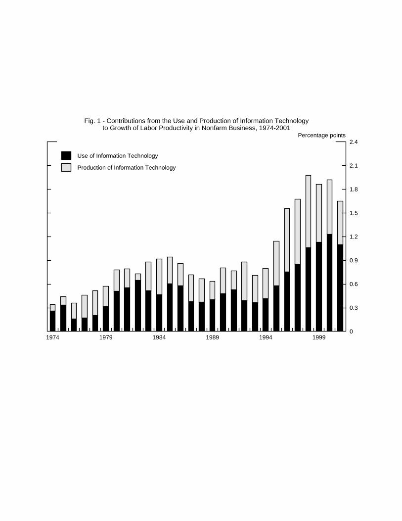
productivity growth after 1995. This large contribution can also be seen in figure 1; the

dark bars show the contribution from the use of IT and the light bars show the

contribution from the production of IT on a year-by-year basis. As the figure shows,

these contributions surged after 1995. Although they dropped back in 2001, the

contributions for that year remain well above those observed before 1995. Based on

these results, we conclude that the latest data confirm the main findings in our earlier

work. Namely, the resurgence in labor productivity is still quite evident in the data, and

information technology appears to have played a central role in this pickup.

Further Comparison to Our Earlier Work

Table 2 compares our latest numbers to those in Oliner and Sichel (2000a).10 The

first column of the table shows contributions to the pickup in labor productivity growth

from our earlier paper, the second column presents estimates through 2000 using the

latest data, and the third column repeats the contributions through 2001 shown in table 1.

In addition to the inclusion of data for 2000, the numbers in the second column differ

10 This table shows separate MFP contributions only for the semiconductor and computer sectors to maintain comparability with our earlier work.

19

from those in the first because there have been several data revisions since our earlier

results were completed.11 As can be seen from these columns, incorporating data for

2000 and revisions for earlier years changed our results relatively little. The contribution

to the productivity pickup from software capital deepening increased, but this was offset

by a more negative contribution from labor quality and a somewhat smaller contribution

from MFP growth.

Extending the results through the recession year 2001 tempers the step-up in labor

productivity growth (line 1), as would be expected given the procyclical behavior of

productivity gains. At the same time, line 2 indicates that the growth contribution from

capital deepening increased with the inclusion of data for 2001. The large implied

contribution in 2001 may seem puzzling in light of the recession-related downturn in

investment spending. However, recall that capital deepening reflects the ratio of capital

services to hours worked. Hours declined in 2001, which � all else equal � boosts the

capital-hours ratio. Also, note that our growth accounting uses annual-average data.

Because investment spending weakened over the course of 2001, annual averaging

smooths this decline relative to the change observed over the four quarters of the year.

Similarly, the Tornquist weighting procedure delays the impact of such changes by using

an average of this year�s and last year�s capital income shares as aggregation weights for

the capital deepening contributions. Thus, some of the effects of the recession on

corporate profits (and hence on the capital income shares) will not show up in our

11 The most important data revisions since we finished the work for Oliner and Sichel (2000a) have been the two annual NIPA revisions released by BEA � which are fully reflected in the latest BLS multifactor productivity data � and the inclusion of official estimates of capital stocks for software. (In our earlier work, we had included our own estimate of software capital stocks.) In addition, we have made some minor adjustments to our estimation procedures, but these changes had relatively small effects.

20

numbers until 2002. Indeed, a back-of-the-envelope calculation suggests that the

contribution of capital deepening will drop back in 2002.12

The final effect of folding in data for 2001 is the noticeably smaller contribution

of MFP to the post-1995 step-up in labor productivity growth (line 9). Virtually the

entire effect resides in the large residual sector consisting of all nonfarm business except

the computer and semiconductor industries (line 12).

Some observers might argue that the very small acceleration of MFP outside these

IT-producing sectors indicates that the productivity benefits of IT have been either

narrowly focused or have been largely reversed over the past year. However, we are not

inclined to accept either interpretation for two reasons. First, the use of IT throughout the

economy has contributed significantly to the pickup in labor productivity growth, quite

apart from developments in IT-producing industries. Second, the much-reduced MFP

acceleration in other industries likely reflected cyclical factors.13 Identifying the

magnitude of such cyclical influences is challenging, and we believe that the trend cannot

be inferred from the average growth rate between 1995 and 2001. The first year of that

period, 1995, was midway through the cycle, while the last year, 2001, was a recession

year.14 Thus, taking an average over 1995-2001 implicitly draws a line from a point at

12 To show this, we calculated capital deepening for 2002 on the assumption that the growth rate of real investment in high-tech equipment snaps back to its robust average pace during 1996-2000 and that hours fall nearly 1 percent in 2002 on an annual-average basis as projected in Macro Advisers� January Economic Outlook. Even under this optimistic assumption for investment and sluggish forecast for hours, the contribution of capital deepening to labor productivity growth in 2002 would be below its 2001 value, but still significantly above its pre-1995 value. 13 Even though MFP is often associated with technological change, short-run movements in MFP can be heavily influenced by cyclical factors that have little relation to technological change. For further discussion of this point, see Basu, Fernald, and Shapiro (2001). 14 Inferring the trend from the average growth rate between 1995 and 2000 also may be problematic because the average covers a period from mid-cycle to peak. But, moving the initial year back to the prior peak in 1990 is not appealing because we are interested in what happened to productivity beginning in the mid-1990s.

21

mid-cycle to a point near the bottom of the cycle. Such a line likely understates the trend

over this period.

5. LABOR PRODUCTIVITY GROWTH IN THE STEADY STATE

How much of the resurgence in labor productivity growth in the second half of the

1990s is sustainable? To address this question, we use the steady-state machinery

described in section 2 to generate a range of likely outcomes for labor productivity

growth in the future. We do not regard these steady-state results as forecasts of

productivity growth for any particular time period. Rather, this exercise yields

�structured guesses� of the sustainable growth in labor productivity consistent with

alternative scenarios for the evolution of key features of the economy.

To construct this range of likely outcomes, we set lower and upper bounds on

steady-state parameters and then solve for the implied rates of labor productivity growth.

We believe that these scenarios encompass the most plausible paths going forward, but

there is substantial uncertainty about future productivity developments. Hence, as we

will discuss, the sustainable pace of labor productivity growth could fall outside the range

that we consider most likely. The rest of this section describes the lower and upper

bound parameter values that we chose, presents our steady-state results, and compares

our results to those obtained by other researchers.

Parameter Values

Table 3 displays the many parameters that feed into our model of steady-state

growth. To provide some historical context, the first three columns of the table show the

average value of each parameter over 1974-90, 1991-95, and 1996-2001. The next two

22

columns present our assumed lower-bound and upper-bound values for each parameter in

the steady state, and the final column briefly indicates the rationale for these steady-state

values.15

Lines 1-15 of the table list the parameters needed to compute aggregate and

sectoral MFP growth in the steady state. These parameters include each sector�s current-

dollar share of nonfarm business output (the µ�s), outlays for semiconductors as a share

of total input costs in each final-output sector (the β�s), the rate of output price inflation

in each sector relative to that in the �other final-output� sector (the π�s), and the growth

of MFP in the �other final output� sector (MFPO).

Although the steady-state bounds for some of these parameters require no

discussion beyond the brief rationale in the table, others need further explanation.16

Starting with the output shares, we calibrated the steady-state bounds from the plots in

figure 2. The short lines in each panel represent the bounds, which can be compared to

the history for each series. The current-dollar output shares for producers of computer

hardware and communication equipment have each fluctuated in a fairly narrow range

since the mid-1980s. Our steady-state bounds largely bracket those ranges. For

producers of software and semiconductors, the current-dollar output shares have trended

sharply higher over time, and our steady-state bounds allow for some additional increase

15 Note that the upper-bound value for each parameter yields a higher rate of productivity growth than the lower-bound value. For some parameters, such as relative prices, the upper-bound value is numerically smaller than the lower-bound value. 16 In performing similar exercises, DeLong (2002), Kiley (2001), and Martin (2001) start with demand elasticities for high-tech products to generate output and income shares. In contrast, we set assumptions for output shares and other key parameters directly. Because relatively little is known about high-tech demand elasticities, we prefer the transparency of directly setting output shares and other parameters based on their historical patterns.

23

from the average level in recent years.17

Among the semiconductor cost shares (the β�s), we set the share for computers

equal to 0.30, the middle of the range employed by Triplett (1996). For software, we set

the share to zero. The share for communication equipment is shown in figure 3. This

share has risen quite a bit since the early 1990s, reflecting the increasing concentration of

computer-like technology in communication equipment. We set the steady-state bounds

on the assumption that this trend will persist.

This increase in the semiconductor content of communication equipment implies

that the relative price for such equipment is likely to fall more rapidly in the future than it

has over history. We built that expectation into the steady-state bounds for πM, shown on

line 14. These values were chosen to ensure that the implied MFP growth rate for the

sector, computed by the dual method, remained close to the average pace over 1996-

2001.

This issue does not arise for the other final-output sectors, where the

semiconductor cost shares are assumed to change little, if at all, going forward. For these

sectors (lines 11-13), we set the bounds on relative price changes (the Π�s) by reference

to historical patterns. The lower bound for each sector equals the average rate of relative

price change over 1974-2001, while the upper bound lies midway between that average

and the most rapid rate of relative price decline for the three subperiods since 1974.

Thus, we do not assume that the extremely rapid declines in computer and semiconductor

prices over 1996-2001 will persist in the steady state, even in our optimistic scenario.

Lines 16-28 of the table list the components of the capital income shares. For the 17 The output share for the semiconductor sector plunged in 2001 to the lowest level since 1994 owing to the deep cutbacks in spending on high-tech equipment during the recession. In setting the steady-state bounds, we assumed that the cyclical drop would be reversed as the economy recovers from recession.

24

nominal rate of return on capital and the asset-specific depreciation rates, we simply

project forward the average values for 1996-2001. These parameters varied only slightly

between the first and second halves of the 1990s; moreover, the higher nominal return on

capital over 1974-90, which was driven in part by the elevated pace of inflation over that

period, is not appropriate for the current low-inflation environment. For the next element

of the income share, the expected capital gain or loss on the asset, we set the steady-state

bounds in essentially the same way as we did for the relative inflation rates. For all types

of capital except communication equipment, we chose these bounds by reference to the

historical data, though we looked back only to 1991 to avoid building in the higher rates

of inflation that prevailed over 1974-90. The bounds for communication equipment were

set to the analogous bounds for the relative price decline on line 14, plus two percentage

points. This add-on for the assumed rate of inflation in the �other final-output� sector

converts the relative price change into an absolute change.

The final piece of the income share is the (tax-adjusted) capital-output ratio,

expressed in current dollars (TpKK/pY). Figure 4 displays this ratio back to 1974 for the

four types of capital. For computer hardware and communication equipment, where the

capital-output ratio has not displayed a clear trend of late, we set the bounds to keep the

ratio in its neighborhood of recent years. In contrast, for software and other fixed capital,

we chose the bounds to allow for a continuation of longer-term trends. Figure 5 shows

the implied bounds for the capital income shares, along with the historical series for these

shares. The one series that bears comment is the share for other equipment and

nonresidential structures, which plummeted in 2001, as the recession-induced decline in

25

corporate profits depressed the nominal return to capital (R).18 The steady-state bounds

for this income share imply at least a partial reversal of this cyclical decline.

The final parameter of note is the growth of labor quality (line 35). We assume

that labor quality will increase 0.30 percent per year in steady state, noticeably slower

than its average annual rise since 1959. Jorgenson, Ho, and Stiroh (2002) suggest a step-

down in labor quality growth of similar magnitude, while Aaronson and Sullivan (2001)

project a slightly larger drop-off in labor quality growth going forward.

Results

Table 4 contains the �structured guesses� of labor productivity growth in the

steady state using lower-bound and upper-bound parameter values.19 As shown on line 1,

the lower-bound parameter values generate steady-state growth in labor productivity of

about 2 percent, while the upper-bound values imply growth of slightly more than 2-¾

percent.20 This range, which sits well above the sluggish pace realized from the early

1970s to the mid-1990s, suggests a relatively optimistic outlook for labor productivity.

To provide intuition for the steady-state range, note that the lower-bound figure of

about 2 percent is roughly ½ percentage point below the pace of labor productivity 18 The drop in R had a much greater effect on the income share for this broad capital aggregate than on the income shares for computers, software, or communication equipment. For these high-tech assets, the rapid trend rate of depreciation is the dominant piece of the gross return, overwhelming even sizable movements in R. 19 As noted in section 2, our model does not explicitly account for adjustment costs. Nevertheless, we recognize that such costs could have important implications for labor productivity growth, as emphasized by Kiley (2001) and Basu, Fernald, and Shapiro (2001). And, implicitly, our steady-state estimates of labor productivity growth embed the average historical value of adjustment costs. Specifically, if adjustment costs have held down labor productivity growth on average historically, our growth-accounting framework will sweep these effects into the residual � which is MFP growth in �other final output.� Because our steady-state estimates depend on MFP growth in that residual category, the average historical magnitude of adjustment costs is implicitly built into these estimates. 20 It is reassuring that the results generated by the steady-state model over historical periods are well aligned with measured productivity growth. In particular, if we use the steady-state model with the historical average parameter values in table 3, it returns an average growth rate for labor productivity of 1.57 percent over 1974-2001, very close to the actual growth rate of 1.62 percent over this period.

26

growth during 1996-2001. This slowdown occurs because we assume that the rates of

decline in semiconductor and computer prices revert to their long-run historical averages

from the very rapid pace realized in the second half of the 1990s. These assumptions

produce a marked slowdown in MFP growth in the semiconductor sector and, to a lesser

extent, in the computer sector. Nonetheless, labor productivity growth for nonfarm

business as a whole remains above the 1974-95 average because the IT sectors, taken

together, constitute a larger part of the economy than they did in this earlier period.

The upper-bound figure of about 2.8 percent in steady state is almost ½

percentage point above the 1996-2001 pace. The model generates this step-up even

though the price declines for semiconductors and computers in steady state (and hence

the rates of MFP growth) are assumed to be less rapid than those in the second half of the

1990s. The countervailing factor is that the semiconductor sector and other IT sectors

grow as a share of the economy compared to the second half of the 1990s. The greater

importance of these sectors with relatively fast MFP growth more than makes up for the

slower price declines for semiconductors and computers.

The remaining lines of table 4 decompose steady-state growth in labor

productivity into induced capital deepening and MFP growth. These numbers highlight

the important role of IT in future labor productivity growth. In particular, a comparison

of lines 2 and 3 indicates that the induced capital deepening in steady state is very heavily

skewed toward IT capital in both the lower- and upper-bound scenarios, just as it was in

the latter half of the 1990s. More broadly, as shown on line 7, the combined contribution

of both the induced use and the production of IT accounts for about three-fourths of

overall labor productivity growth in both the lower- and upper-bound scenarios.

27

As indicated above, our intent is to provide a likely range for steady-state growth

in labor productivity, not to bound all possible outcomes. For example, the steady-state

model can generate labor productivity growth above 3 percent per year if we assume that

semiconductor and computer prices continue to fall at the 1996-2001 pace and allow the

semiconductor output share to rise by the amount seen between the first and second

halves of the 1990s. Conversely, we can generate numbers for labor productivity growth

between 1-½ and 1-¾ percent per year if we assume that price declines for computers and

semiconductors revert to their historical average and that the computer and

semiconductor output shares go back down to levels seen in the first half of the 1990s.

So, while we are comfortable with a likely range for steady-state labor productivity

growth from 2 percent to 2-¾ percent, we are well aware of the uncertainty that attends

the exercise we have undertaken.

Comparison to Other Research

Table 5 compares the steady-state results in this paper to those obtained by other

researchers. There are two points to take away from this table. First, the range of

estimates is very wide, extending from about 1-¼ percent up to 3-¼ percent. This range

highlights the uncertainty surrounding the future path of productivity growth. Second,

despite the wide band of uncertainty, most of the point estimates (or range midpoints) fall

within our range of 2 to 2-¾ percent per year. Thus, there is considerable agreement

among researchers that productivity growth likely will remain fairly strong going

forward.

28

6. CONCLUSION

Recent debates about the pickup of productivity growth in the United States have

revolved around two questions. First, are the results from earlier research that

emphasized the role of IT still valid given the sharp contraction in the technology sector?

Second, how much of the improvement in labor productivity growth since the mid-1990s

could plausibly be sustained? This paper addressed both questions.

As for the robustness of earlier results, we used data through 2001 to reassess the

role of information technology in the productivity revival since the mid-1990s. These

new growth-accounting results indicate that the story told in Oliner and Sichel (2000a)

still stands. Namely, output per hour accelerated substantially after 1995, driven in large

part by greater use of IT capital goods by businesses all throughout the economy and by

more rapid efficiency gains in the production of IT goods.

To address the question of sustainability, we analyzed the steady-state properties

of a multi-sector growth model. This framework translates alternative views about the

evolution of the technology sector and other features of the economy into estimates of

labor productivity growth in the steady state. When we imposed relatively conservative

values for key parameters, this framework generated steady-state growth in labor

productivity of about 2 percent per year. This estimate rose to roughly 2-¾ percent when

we imposed somewhat more optimistic assumptions. We refer to these estimates as

structured guesses, and think of them as identifying a likely range of productivity

outcomes over roughly the next decade. Of course, any such exercise entails substantial

uncertainty, and we also discussed scenarios that would generate a wider range of

outcomes.

29

Our analysis highlights that future increases in output per hour will depend

importantly on the pace of technological advance in the semiconductor industry and on

the extent to which products embodying these advances diffuse through the economy.

This observation is consistent with the emphasis in Jorgenson (2001) on semiconductor

technology. Gaining a deeper understanding of technological developments in this sector

should be a high priority for those attempting to shed light on trends in productivity.

30

REFERENCES

Aaronson, Daniel and Daniel Sullivan. 2001. Growth in worker quality. Federal Reserve Bank of Chicago Economic Perspectives 25, Fourth Quarter: 53-74. Aizcorbe, Ana. 2002. Why are semiconductor prices falling so fast? Industry estimates and implications for productivity measurement. Federal Reserve Board. Finance and Economics Discussion Series Paper 2002-20. March. <www.federalreserve.gov/pubs/feds/200220/200220pap.pdf>. Baily, Martin Neil. 2002. The new economy: Post mortem or second wind? Institute for International Economics. Unpublished paper. January 10. Basu, Susanto, John G. Fernald, and Matthew D. Shapiro. 2001. Productivity growth in the 1990s: Technology, utilization, or adjustment? Carnegie-Rochester Conference Series on Public Policy 55: 117-165. Bosworth, Barry P. and Jack E. Triplett. 2000. What is new about the new economy? Information technology, economic growth, and productivity. Unpublished paper. The Brookings Institution. Congressional Budget Office. 2002. The Budget and Economic Outlook: Fiscal Years 2003-2012. January. <www.cbo.gov>. (Accessed: March 26, 2002). DeLong, J. Bradford. 2002. Productivity growth in the 2000s. Unpublished paper. University of California at Berkeley. Domar, Evsey. 1961. On the measurement of technological change. Economic Journal 71, December: 309-29. Doms, Mark. 2002. Communications equipment: What has happened to prices? Unpublished paper. Federal Reserve Board. Economic Report of the President. 2002. Washington, D.C.: U.S. Government Printing Office. Economic Report of the President. 1999. Washington, D.C.: U.S. Government Printing Office. Flamm, Kenneth. 1997. More for less: The economic impact of semiconductors. December. Semiconductor Industry Association. Fraumeni, Barbara M. 1997. The measurement of depreciation in the U.S. national income and product accounts. Survey of Current Business 77, July: 7-23.

31

Gordon, Robert J. 2002. Technology and economic performance in the American economy. National Bureau of Economic Research. Working paper no. 8771. Gordon, Robert J. 2000. Does the �new economy� measure up to the great inventions of the past? Journal of Economic Perspectives 14, Fall: 49-74. Grimm, Bruce. 1998. Price indexes for selected semiconductors, 1974-96. Survey of Current Business 78, February: 8-24. Herman, Shelby. 2000. Fixed assets and consumer durable goods. Survey of Current Business 80, April: 17-30. Hulten, Charles R. 1978. Growth accounting with intermediate inputs. The Review of Economic Studies 45, October: 511-18. Jorgenson, Dale W. 2001. Information technology and the U.S. economy. American Economic Review 91, March: 1-32. Jorgenson, Dale W. and Kevin J. Stiroh. 2000. U.S. economic growth in the new millenium. Brookings Papers on Economic Activity 1, pp. 125-211. Jorgenson, Dale W., Mun S. Ho, and Kevin J. Stiroh. 2002. Projecting productivity growth: Lessons from the U.S. growth resurgence. This volume. Kiley, Michael T. 2001. Computers and growth with frictions: Aggregate and disaggregate evidence. Carnegie-Rochester Conference Series on Public Policy 55: 171-215. Macroeconomic Advisers. 2002. Economic Outlook. St. Louis, Missouri. January. Martin, Bill. 2001. American potential. UBS Asset Management. May. <www.phillipsdrew.com/research/american_potential.pdf>. (Accessed: March 26, 2002). McKinsey Global Institute. 2001. US productivity growth 1995-2000: Understanding the contribution of information technology relative to other factors. Washington, D.C.: McKinsey Global Institute. October. Moylan, Carol. 2001. Estimation of software in the U.S. national accounts: New developments. Organization for Economic Cooperation and Development, STD/NA(2001)25, September 24, 2001. Oliner, Stephen D. 1994. Measuring stocks of computer peripheral equipment: Theory and application. Unpublished paper. Federal Reserve Board.

32

Oliner, Stephen D. and Daniel E. Sichel. 2000a. The resurgence of growth in the late 1990s: Is information technology the story? Journal of Economic Perspectives 14, Fall: 3-22. Oliner, Stephen D. and Daniel E. Sichel. 2000b. The resurgence of growth in the late 1990s: Is information technology the story? Federal Reserve Board. Finance and Economics Discussion Series Paper 2000-20. May. <www.federalreserve.gov/pubs/feds/2000/200020/200020pap.pdf>. Parker, Robert and Bruce Grimm. 2000. Software prices and real ouptut: Recent developments at the Bureau of Economic Analysis. Bureau of Economic Analysis. Unpublished paper. April. Roberts, John M. 2001. Estimates of the productivity trend using time-varying parameter techniques. Contributions to Macroeconomics 1, no. 1. <www.bepress.com/bejm/contributions/vol1/iss1/art3>. (Accessed: March 26, 2002). Sichel, Daniel E. 1997. The Computer Revolution: An Economic Perspective. Washington, D.C.: The Brookings Institution. Solow, Robert. 1957. Technical change and the aggregate production function. Review of Economics and Statistics 39, August: 65-94. Steindel, Charles and Kevin J. Stiroh. 2001. Productivity growth: What is it and why do we care about it? Business Economics 36, October: 13-31. Triplett, Jack E. 1996. High-tech industry productivity and hedonic price indices. In Industry Productivity: International Comparison and Measurement Issues, Proceedings of May 2-3, 1996 OECD workshop, 119-42. Paris: Organisation for Economic Cooperation and Development. Whelan, Karl. 2001. A two-sector approach to modeling U.S. NIPA data. Federal Reserve Board. Finance and Economics Discussion Series Paper 2001-4. April. <www.federalreserve.gov/pubs/feds/2001/200104/200104pap.pdf>. Whelan, Karl. 2000. Computers, obsolescence, and productivity. Federal Reserve Board. Finance and Economics Discussion Series Paper 2000-6. February. <www.federalreserve.gov/pubs/feds/2000/200006/200006pap.pdf>. Whelan, Karl. 1999. Tax incentives, material inputs, and the supply curve for capital equipment. Federal Reserve Board. Finance and Economics Discussion Series Paper 1999-21. April. <www.federalreserve.gov/pubs/feds/1999/199921/199921pap.pdf>.

Table 1

Contributions to Growth in Labor Productivity, Using Latest Data 1974- 1991- 1996- Post-1995 1990 1995 2001 change (1) (2) (3) (3) minus (2) 1. Growth of labor productivity1 1.36 1.54 2.43 .89 Contributions from:2 2. Capital deepening .77 .52 1.19 .67 3. Information technology capital .41 .46 1.02 .56 4. Computer hardware .23 .19 .54 .35 5. Software .09 .21 .35 .14 6. Communication equipment .09 .05 .13 .08 7. Other capital .37 .06 .17 .11 8. Labor quality .22 .45 .25 -.20 9. Multifactor productivity .37 .58 .99 .41 10. Semiconductors .08 .13 .42 .29 11. Computer hardware .11 .13 .19 .06 12. Software .04 .09 .11 .02 13. Communication equipment .04 .06 .05 -.01 14. Other sectors .11 .17 .23 .06 Memo: 15. Total IT contribution3 .68 .87 1.79 .92 1. In the nonfarm business sector. Measured as average annual log difference for years shown multiplied by 100. 2. Percentage points per year. 3. Equals the sum of lines 3 and 10-13. Note: Detail may not sum to totals due to rounding. Source: Authors� calculations based on BEA and BLS data.

Table 2

Acceleration in Labor Productivity between 1991-95 and Post-1995 Period, Effect of New Data and Revisions

JEP Paper This Paper This Paper Through 1999 Through 2000 Through 2001 1. Acceleration in labor productivity1 1.04 1.00 .89 Contributions from:2 2. Capital deepening .48 .57 .67 3. Information technology capital .45 .54 .56 4. Computer hardware .36 .36 .35 5. Software .04 .13 .14 6. Communication equipment .05 .07 .08 7. Other capital .03 .02 .11 8. Labor quality -.13 -.20 -.20 9. Multifactor productivity .68 .62 .41 10. Semiconductors .27 .30 .29 11. Computer hardware .10 .06 .06 12. Other sectors3 .31 .26 .06 1. In the nonfarm business sector. Measured as percentage points per year. 2. Percentage points per year. 3. Includes producers of communication equipment and software. Note: Detail may not sum to totals due to rounding. Source: Authors� calculations based on BEA and BLS data.

Table 3

Parameter Values for Steady-State Calculations . Historical Averages Steady-State Values 1974- 1991- 1996- Lower Upper Method for Setting Parameter 1990 1995 2001 Bound Bound Steady-State Values . Output shares1 (µ) 1. Computer hardware 1.06 1.19 1.32 1.10 1.40 See figure 2. 2. Software .84 1.79 2.70 3.10 3.60 See figure 2. 3. Communication equipment 1.80 1.68 1.83 1.60 2.00 See figure 2. 4. Other final-output sectors 96.33 95.45 94.14 94.20 93.00 Implied by lines 1-3 and 5. 5. Net exports of semiconductors -.04 -.11 .00 .00 .00 1996-2001 average. 6. Total semiconductor output .30 .58 .91 1.00 1.20 See figure 2. Semiconductor cost shares1 (β) 7. Computer hardware 30.00 30.00 30.00 30.00 30.00 Assumed constant value. 8. Software .00 .00 .00 .00 .00 Assumed constant value. 9. Communication equipment 1.17 4.59 8.88 13.00 16.00 See figure 3. 10. Other final-output sectors .00 .27 .37 .46 .46 Implied by lines 1-4, 6-9, and 36. Relative inflation rates2 (π) 11. Semiconductors -28.90 -21.75 -44.71 -31.01 -37.86 � �Lower bound is 1974-2001 average; 12. Computer hardware -19.29 -17.79 -27.15 -20.71 -23.93 �� � upper bound is midway between that 13. Software -4.13 -4.83 -3.90 -4.21 -4.52 � �value and fastest historical decline. 14. Communication equipment -2.44 -4.06 -5.80 -6.00 -7.75 Calibrated to keep the sector�s MFP growth rate near the 1996-2001 pace. 15. Growth of MFPO

3 .11 .17 .23 .11 .23 Used historical range. . Footnotes are at the end of the table.

Table 3, continued . Historical Averages Steady-State Values 1974- 1991- 1996- Lower Upper Method for Setting Parameter 1990 1995 2001 Bound Bound Steady-State Values . 16. Nominal return on capital3 (R) 7.88 4.29 4.55 4.55 4.55 1996-2001 average. Depreciation rates3 (δ) 17. Computer hardware 29.74 30.11 30.30 30.30 30.30 1996-2001 average. 18. Software 34.87 37.04 38.46 38.46 38.46 1996-2001 average. 19. Communication equipment 13.00 13.00 13.00 13.00 13.00 1996-2001 average. 20. Other business fixed capital 5.87 6.08 6.10 6.10 6.10 1996-2001 average. Expected capital gains/losses4 (Π) 21. Computer hardware -12.70 -11.79 -23.21 -17.50 -20.36 See footnote 5. 22. Software 3.27 -.56 -.31 -.44 -.50 See footnote 5. 23. Communication equipment 3.65 -.07 -3.01 -4.00 -5.75 See footnote 6. 24. Other business fixed capital 6.31 2.52 2.55 2.54 2.53 See footnote 5. Capital-output ratios (TpKK /pY) 25. Computer hardware .0192 .0293 .0294 .0300 .0360 See figure 4. 26. Software .0191 .0440 .0618 .0800 .0900 See figure 4. 27. Communication equipment .0876 .1087 .0951 .0875 .1025 See figure 4. 28. Other business fixed capital 2.4227 2.2648 2.1008 1.9000 2.0500 See figure 4. . Footnotes are at the end of the table.

Table 3, continued . Historical Averages Steady-State Values 1974- 1991- 1996- Lower Upper Method for Setting Parameter 1990 1995 2001 Bound Bound Steady-State Values .

Income shares1 (α) 29. Computer hardware .92 1.34 1.71 1.57 1.99 Implied. See figure 5. 30. Software .75 1.85 2.67 3.48 3.92 Implied. See figure 5. 31. Communication equipment 1.48 1.88 1.96 1.89 2.39 Implied. See figure 5. 32. Other business fixed capital 18.00 17.78 17.04 15.42 16.65 Implied. See figure 5. 33. Other capital7 9.81 8.90 8.93 8.93 8.93 1996-2001 average. 34. Labor 69.04 68.25 67.69 68.72 66.13 Implied by lines 29-33.

Other parameters 35. Growth of labor quality3 (q) .32 .65 .38 .30 .30 Assumed slower growth. 36. Ratio of domestic semiconductor .89 .86 1.03 1.03 1.03 1996-2001 average. output to domestic use (1+θ) . 1. Current-dollar shares, in percent. 2. Output price inflation in each sector minus that in the �other final-output� sector, in percentage points. 3. In percent. 4. Three-year moving average of price inflation for each asset, in percent. 5. Lower bound is average over 1991-2001; upper bound is midway between that value and the smaller of the 1991-1995 and 1996-2001 values. 6. The lower and upper bounds equal the corresponding values for the relative inflation rate of communication equipment (line 14), plus 2 percent � the assumed rate of inflation in the �other final-output� sector. 7. Includes land, inventories, and tenant-occupied housing.

Table 4

Steady-State Results Using Lower Using Upper Bound Parameters Bound Parameters 1. Growth of labor productivity1 1.98 2.84 Contributions from:2 2. Induced capital deepening .97 1.47 3. Information technology capital .88 1.31 4. Other capital .09 .16 5. Labor quality .30 .30 6. Multifactor productivity .72 1.07 Memo: 7. Total IT contribution3 1.50 2.17 1. In the nonfarm business sector; measured in percent. 2. Percentage points per year. 3. Equals line 3 plus the contributions included in line 6 from producers of computer hardware, software, communication equipment, and semiconductors.

Note: Detail may not sum to totals due to rounding.

Table 5

Alternative Estimates of Steady-State Growth in Labor Productivity (Percent per year)

Point Estimate Range 1. This paper 2.0 to 2.8 2. Jorgenson, Ho, and Stiroh (2002)1 2.25 1.3 to 3.0 3. Congressional Budget Office (2002)2 2.2 4. Economic Report of the President (2002) 3 2.1 5. Baily (2002) 2.0 to 2.5 6. Gordon4 2.0 to 2.2 7. Kiley (2001) 2.6 to 3.2 8. Martin (2001)5 2.75 2.5 to 3.0 9. McKinsey (2001)6 ≈ 2.0 1.6 to 2.5 10. Roberts7 2.6 11. DeLong (2002) �like the fast-growing late 1990s� 1. Jorgenson, Ho, and Stiroh measure productivity growth for a broader definition of the economy than do the other papers. To make their numbers comparable to those in the other studies, add 0.15 percentage point to the point estimate and range shown for Jorgenson, Ho, and Stiroh in the table. 2. Table 2-5. 3. Table 1-2, p. 55. 4. Based on personal correspondence with Robert Gordon, March 24, 2002. 5. In personal correspondence of March 23, 2002, Bill Martin indicated that his forthcoming revised estimates would be slightly lower than those in Martin (2001). 6. Chapter 3, exhibit 13. 7. Unpublished update to Roberts (2001).

Use of Information Technology

Production of Information Technology

1974 1979 1984 1989 1994 19990

0.3

0.6

0.9

1.2

1.5

1.8

2.1

2.4

Fig. 1 - Contributions from the Use and Production of Information Technology

Percentage pointsto Growth of Labor Productivity in Nonfarm Business, 1974-2001

Figure 2Current-dollar Output Shares (percent)

Computer Hardware

0

0.5

1

1.5

2

1974 1978 1982 1986 1990 1994 1998

Software

0

1

2

3

4

1974 1978 1982 1986 1990 1994 1998

Figure 2 (cont.)Current-Dollar Output Shares (percent)

Communication Equipment

0

0.5

1

1.5

2

2.5

1974 1978 1982 1986 1990 1994 1998

Semiconductors

0

0.5

1

1.5

1974 1978 1982 1986 1990 1994 1998

Figure 3Semiconductor Cost Share in Communication

Equipment (percent)

0

4

8

12

16

1974 1978 1982 1986 1990 1994 1998 2002

1Each subcomponent within a category is tax-weighted.

Figure 41

Current-dollar Capital-Output Ratios

Computer Hardware

0

0.01

0.02

0.03

0.04

1974 1978 1982 1986 1990 1994 1998 2002

Software

0

0.025

0.05

0.075

0.1

1974 1978 1982 1986 1990 1994 1998 2002

1Each subcomponent within a category is tax-weighted.

Figure 4 (cont.)1

Current-dollar Capital-Output Ratios

Communication Equipment

0.025

0.05

0.075

0.1

0.125

1974 1978 1982 1986 1990 1994 1998 2002

Other Equipment and Nonresidential Structures

1.5

2

2.5

3

1974 1978 1982 1986 1990 1994 1998 2002

Figure 5Current-dollar Income Shares (percent)

Computer Hardware

0

0.5

1

1.5

2

2.5

1974 1978 1982 1986 1990 1994 1998 2002

Software

0

1

2

3

4

1974 1978 1982 1986 1990 1994 1998 2002

Other Equipment and Nonresidential Structures

12

14

16

18

20

1974 1978 1982 1986 1990 1994 1998 2002

Figure 5 (cont.)Current-dollar Income Shares (percent)

Communication Equipment

0.5

1

1.5

2

2.5

1974 1978 1982 1986 1990 1994 1998 2002

1

APPENDIX 1: MODEL OF SECTORAL PRODUCTIVITY

This appendix presents our model of sectoral productivity and derives key results

for our analysis of growth in aggregate labor productivity. The model divides nonfarm

business into five sectors. Four of the sectors produce final output (computer hardware,

software, communication equipment, and all other final output). The fifth sector

produces semiconductors, which are either consumed as an intermediate input by the

final-output sectors or exported to foreign firms. To focus on essential linkages, the

model abstracts from all intermediate inputs besides semiconductors.

The Model

Let Yi (i = 1,�,4) denote the production of the final-output sectors. Each sector

produces investment goods (Ii) and consumption goods (Ci) for domestic use, where Ii

and Ci are identical goods sold to different agents (firms buy Ii, while households buy Ci).

Let Ii,j and Ii,s denote, respectively, the purchases of Ii by final-output sector j (j = 1,�,4)

and by semiconductor producers, with Ii = � j Ii,j + Ii,s. Each sector also produces goods

for export (Xi). To produce this output, sector i employs labor (Li) and various types of

capital (Kj,i, j = 1,�,4), and it purchases semiconductors (Si) as an intermediate input.1

With this notation, the production function for each final-output sector can be written as

(1) Yi = Ci + �=

4

1i

Ii,j + Ii,s + Xi = Fi (Li , K1,i , K2,i , K3,i , K4,i , Si , zi) for i = 1,�,4,

where zi measures the level of multifactor productivity. Although we do not explicitly

model foreign production, the capital stocks Kj,i should be regarded as including 1When either I or K has a double subscript, the first subscript indicates the sector that produced the investment good, while the second subscript indicates the sector that uses it as an input to production.

2

imported capital goods of type j. To ease the notational burden, we have suppressed time

subscripts in equation 1 and will do so throughout this appendix.

The output of the semiconductor sector (Ys) is either sold as intermediate input to

the domestic final-output sectors (Sd) or is exported (Sx). The semiconductors purchased

by the domestic final-demand sectors (Si) include imported semiconductors (Sm), which

implies that the production sold for domestic use can be written as Sd = � i Si - Sm. We

assume that semiconductor producers employ labor and the same set of capital inputs as

the final-output sectors. With these assumptions,

(2) Ys = Sd + Sx = �=

4

1iiS + Sx - Sm = Fs (Ls , K1,s , K2,s , K3,s , K4,s , zs).

The next step is to define the relationship between the sectoral variables and their

aggregate counterparts. Following the guidance of index number theory, we express the

growth in aggregate final output as a superlative index of growth in sectoral final output.

Let •Z ≡ (�Z/�t)/Z denote the growth in any variable Z. Then, the growth of aggregate

nonfarm business output (Y) in our model is

(3) •Y = �

=

4

1i

•

ii Yµ + •

xxS S,µ - •

mmS S,µ

where iµ ≡ piYi /pY (for i = 1,�,4), xS ,µ ≡ psSx /pY, mS ,µ ≡ psSm /pY, and

pY ≡ �=

4

1i

piYi + psSx - psSm.2 pi and ps denote the prices of final output and

semiconductors, respectively, and pY represents aggregate current-dollar output.

2 Equation 3 is just one of several possible superlative indexes of output growth. It differs slightly from the Fisher chain index used in the U.S. National Income and Product Accounts.

3

Equation 3 expresses the growth in aggregate output as a share-weighted average of

sectoral output growth, where the shares are in current dollars. Note that the

semiconductors sold to domestic final-output sectors are an intermediate input for those

sectors and thus do not appear in equation 3; only net exports of semiconductors enter the

equation, consistent with the treatment of semiconductors in the National Income and

Product Accounts.

The definition of labor and capital aggregates in our model is very simple. We

assume that labor input used in a given sector is identical to that used in any other sector.

We also impose this assumption on each type of capital. Given these assumptions, we

can directly aggregate the sectoral inputs, without the need for superlative aggregation

formulas. That is,

(4) L = �=

4

1i

Li + Ls

(5) Kj = �=

4

1i

Kj,i + Kj,s for j = 1,�,4.

Moreover, with this setup, there is a common wage rate (w) for labor in every sector and,

likewise, a common rental rate (rj) for all capital of type j.

Labor input in each sector is the product of hours worked (Hi) and labor quality

(qi), where quality reflects the characteristics of the workers employed in that sector. We

allow labor quality to change over time, but given our assumption of identical labor input

across sectors, qi must equal a common value q in every sector at a given point in time.

Using equation 4, this implies that

4

(6) L = �=

4

1i

q Hi + qHs = qH,

where H represents aggregate hours worked.

To derive the growth-accounting equation for each sector, we impose the standard

neoclassical assumptions of perfect competition and constant returns to scale. We also

assume that there are no adjustment costs. Under these assumptions, profit-maximizing

firms will set the marginal revenue product of each input equal to its one-period cost:

(7) w = ps(�Fs/�Ls) = pi(�Fi /�Li) for i = 1,�,4

(8) rj = ps(�Fs/�Kj,s) = pi(�Fi /�Kj,i) for i, j = 1,�,4

(9) ps = pi(�Fi /�Si) for i = 1,�,4.

If we totally differentiate equations 1 and 2 and then impose conditions 7 through

9, we obtain the standard growth-accounting equations:

(10) •

iY = •

iL

i Lβ + �=

4

1j

•

ijK

ij K ,,β + •

iSi Sβ +

•

iMFP for i = 1,�,4

(11) •

SY = •

SL Lγ + �

=

4

1j

•

SjKj K ,γ +

•

SMFP

where •

iMFP ≡ (�Fi /�zi)/Fi, •

SMFP ≡ (�Fs /�zs)/Fs, and the β�s and γ�s represent the

following income shares: Liβ ≡ wLi /piYi , the labor share in sector i; K

ij ,β ≡ rjKj,i /piYi , the

share for capital of type j in sector i; Siβ ≡ psSi /piYi , the semiconductor share in sector i;

Lγ ≡ wLs /psYs , the labor share in the semiconductor sector; and Kjγ ≡ rjKj,s /psYs , the

share for capital of type j in the semiconductor sector. Given the assumption of constant

returns, the income shares in each sector sum to one.

5

Aggregate Labor Productivity

Proposition 1 derives the expression for growth in aggregate labor productivity in

our model.

Proposition 1

Assume that all markets are perfectly competitive, that production exhibits constant

returns to scale in every sector, and that input use is not subject to adjustment costs.

Then, in the model described by equations 1 through 11, the growth-accounting equation

for aggregate labor productivity is

•Y -

•H = �

=

4

1j

Kjα (

•

jK - •

H ) + •qLα +

•MFP ,

where

•MFP = �

=

4

1i

•

ii MFPµ + •

SS MFPµ

and Lα = wL /pY ; Kjα = rjKj /pY ; iµ = piYi /pY ; and Sµ = psYs /pY.

Proof.

To begin, substitute the expression for •

iY from equation 10 into equation 3:

(12) •Y = �

=

4

1iiµ [ •

iL

i Lβ + �=

4

1j

•

ijK

ij K ,,β + •

iSi Sβ +

•

iMFP ] + •

xxS S,µ - •

mmS S,µ

= �=

4

1i

Lα ( LLi )•

iL + �=

4

1j

�=

4

1i

Kjα ( jij KK , )

•

ijK , + �=

4

1i

Sµ ( Si YS )•

iS

+ �=

4

1i

•

ii MFPµ + •

xxS S,µ - •

mmS S,µ

where the second equality follows (after some algebra) from the definitions of the α�s,

6

β�s, and µ�s. Next, totally differentiate equation 2 to obtain

(13) •

SY = �=

4

1i

( Si YS )•

iS + ( Sx YS )•

xS - ( Sm YS )•

mS .

Multiplying equation 13 by Sµ and using the definitions of Sµ , xS ,µ , and mS ,µ ,

(14) �=

4

1iSµ ( Si YS )

•

iS = •

SS Yµ - •

xxS S,µ + •

mmS S,µ .

Now, substitute equation 14 into equation 12, which yields

(15) •Y = Lα �

=

4

1i

( LLi )•

iL + �=

4

1j

Kjα �

=

4

1i

( jij KK , )•

ijK , + �=

4

1i

•

ii MFPµ + •

SS Yµ .

Next, totally differentiate equations 4 and 5:

(16) •L = �

=

4

1i

( LLi )•

iL + ( LLS )•

SL

(17) •

jK = �=

4

1i

( jij KK , )•

ijK , + ( jSj KK , )•

SjK , ,

and substitute these equations into 15:

(18) •Y = Lα [ •

L - ( LLS )•

SL ] + �=

4

1j

Kjα [ •

jK - ( jSj KK , )•

SjK , ] + �=

4

1i

•

ii MFPµ + •

SS Yµ .

= •LLα + �

=

4

1j

•

jKj Kα + �

=

4

1i

•

ii MFPµ

+ Sµ [ •

SY - ( SL µα )( LLS )

•

SL - �=

4

1j

( SKj µα )( jSj KK , )

•

SjK , ]

= •LLα + �

=

4

1j

•

jKj Kα + �

=

4

1i

•

ii MFPµ + Sµ [ •

SY - •

SL Lγ - �

=

4

1j

•

SjKj K ,γ ]

= •LLα + �

=

4

1j

•

jKj Kα + �

=

4

1i

•

ii MFPµ + •

SS MFPµ ,

7

where the third equality follows from the definitions of the α�s, γ�s, and µ�s, and the

fourth equality follows from equation 11. To complete the proof, recall that •L =

•H +

•q

from equation 6 and that the α�s sum to one under constant returns to scale. Hence,

(19) •LLα = Lα (

•H +

•q ) =

•H - �

=

4

1j

•

HKjα +

•qLα .

Substitute equation 19 into 18, which produces

(20) •Y -

•H = �

=

4

1j

Kjα (

•

jK - •

H ) + •qLα + �

=

4

1i

•

ii MFPµ + •

SS MFPµ . ����

More on Aggregate MFP

Proposition 1 showed that aggregate MFP growth in our model equals a share-

weighted sum of MFP growth in each sector. This result can be rewritten to highlight the

input-output connections between semiconductor producers and the final-output sectors.

In effect, we can integrate semiconductor producers with the final-output sectors that they

supply.

Proposition 2

Under the assumptions of Proposition 1,

•MFP = �

=

4

1i

•

ii MFPµ + •

SS MFPµ = �=

4

1iiµ [ •

iMFP + Siβ (1 + θ )

•

SMFP ] ,

where 1 + θ = �=

4

1iiS SY , the ratio of domestic semiconductor output to domestic use of

semiconductors.

8

Proof.

Using equation 2 and recalling the definitions of iµ , Siβ , xS ,µ , and mS ,µ ,

(21) ≡Sµ SSYp /pY = Sp [�=

4

1iiS + Sx - Sm] /pY

= �=

4

1i

( iiYp /pY)( iS Sp / iiYp ) + Sp (Sx - Sm) /pY = �=

4

1i

Sii βµ + xS ,µ - mS ,µ .

Note that xS ,µ - mS ,µ can be written as Sµ ( Sx - Sm) / SY , so that equation 21 becomes

(22) Sµ = �=

4

1i

Sii βµ / [ 1 - ( Sx - Sm) / SY ] = �

=

4

1i

Sii βµ / [�

=

4

1iiS / SY ] = �

=

4

1i

Sii βµ ( 1 + θ ),

where the second equality follows from equation 2 and the third from the definition

1 + θ ≡ �=

4

1iiS SY . Finally, substitute equation 22 into the expression from Proposition

1 for growth in aggregate MFP:

(23) •

MFP = �=

4

1i

•

ii MFPµ +•

SS MFPµ = �=

4

1iiµ [ •

iMFP + Siβ (1 + θ )

•

SMFP ]. ����

Measuring Sectoral MFP

To make use of propositions 1 and 2, we need to estimate MFP growth in each

sector. This can be done either from the sectoral production functions, as in equations 10

and 11, or from the sectoral cost functions � the �dual� approach. We opt for the dual

approach because the required data are more readily available. The dual counterparts to

equations 10 and 11 are:

(24) •

ip = •wL

iβ + �=

4

1j

•

jK

ij r,β + SS

i p•

β - •

iMFP for i = 1,�,4

9

(25) •

Sp = •wLγ + �

=

4

1j

•

jKj rγ -

•

SMFP .

These equations state that the growth in each sector�s output price equals the growth in

the share-weighted average of its input costs, minus the growth in MFP. MFP growth

enters with a negative sign because efficiency gains hold down a sector�s output price

given its input costs.

To reduce the amount of data needed to estimate MFP growth from equations 24

and 25, we assume that every sector has the same labor and capital shares up to a scaling

factor that reflects the intensity of semiconductor use. That is,

(26) S

L

1

1

1 ββ−

= � = S

L

4

4

1 ββ−

= Lγ and S

Kj

1

1,

1 ββ−

= � = S

Kj

4

4,

1 ββ−

= Kjγ for j = 1,�,4.

One can easily verify that the restricted factor shares sum to one in each sector. Also,

given equation 26, one can show (with some algebra) that Lγ = Lα and Kjγ = K

jα � that is,

the income shares for aggregate nonfarm business equal their counterparts in the

semiconductor sector. Substituting equation 26 into 24 and making use of the

correspondence between the γ�s and the α�s, we obtain

(27) •

ip = (1 - Siβ )[ •

wLα + �=

4

1j

•

jKj rα ] + S

Si p

•β -

•

iMFP for i = 1,�4.

Let •

V ≡(•wLα + �

=

4

1j

•

jKj rα ) denote the share-weighted growth in labor and capital costs

for the nonfarm business sector as a whole. Substitute •

V into the dual equations 25 and

27, noting that Lγ = Lα and Kjγ = K

jα in equation 25. The result is:

(28) •

ip = (1 - Siβ )

•V +

•

SSi pβ -

•

iMFP for i = 1,�,3

10

(29) •

4p = (1 - S4β )

•V +

•

SS p4β -

•

4MFP

(30) •

Sp = •

V - •

SMFP

where we have specifically identified sector 4, which will serve as the numeraire sector.

We now use the dual equations to derive expressions for MFP growth in two

cases. In the first case, we infer the rates of sectoral MFP growth that are consistent with

an independent estimate of aggregate MFP growth (from the Bureau of Labor Statistics).

This case represents the methodology we use to compute growth contributions through

2001. In the second case, which we use for our steady-state analysis, we solve for

aggregate MFP growth and MFP growth in sectors 1 through 3, conditional on an

assumed pace of MFP growth in sector 4. The next proposition derives the expressions

for sectoral MFP growth in both cases.

Proposition 3

Let Sπ ≡•

Sp - •

4p and iπ ≡•

ip - •

4p (i = 1,�,3) denote the rate of change in each sector�s

output price relative to that in sector 4. Given the dual equations 28-30, the solutions for

sectoral and aggregate MFP growth are as follows.

Case I: Conditioning on Aggregate MFP Growth

•

4MFP = (1 - S4β )(

•MFP + �

=

3

1iiiπµ ) + [ S

4β + (1 - S4β )(1 - �

=

4

1iiµ ) ] Sπ

•

SMFP = (•

4MFP - Sπ ) /(1 - S4β )

•

iMFP = •

4MFP - iπ - ( Siβ - S

4β )•

SMFP for i = 1,�,3

11

Case II: Conditioning on MFP Growth in Sector 4

•

SMFP = (•

4MFP - Sπ ) /(1 - S4β )

•

iMFP = •

4MFP - iπ - ( Siβ - S

4β )•

SMFP for i = 1,�,3

•MFP = �

=

4

1i

•

ii MFPµ + •

SS MFPµ

Proof.

The proof for case II is nearly immediate. Subtract equation 29 from equations 28

and 30. After rearranging terms and using equation 30 to substitute•

SMFP for •

V - •

Sp ,

we obtain:

(31) •

iMFP = •

4MFP - iπ - ( Siβ - S

4β )•

SMFP for i = 1,�,3

(32) •

SMFP = (•

4MFP - Sπ ) /(1 - S4β ).

Equations 31 and 32, plus the expression for •

MFP derived in proposition 1, establish the

results for case II. Note that the solution is recursive � first solve for•

SMFP from

equation 32, then substitute the result into equation 31, and finally substitute all the

sectoral MFP growth rates into the expression for aggregate MFP growth.

To prove the result for case I, substitute equations 31 and 32 into the expression

for aggregate MFP growth. After rearranging terms, this yields:

(33) •

MFP = �=

4

1i

•

ii MFPµ + •

SS MFPµ

12

= [�=

4

1iiµ + [ Sµ -�

=

3

1iiµ ( S

iβ - S4β )]/(1 - S

4β )] •

4MFP

- �=

3

1iiiπµ - [[ Sµ - �

=

3

1iiµ ( S

iβ - S4β )]/(1 - S

4β )] Sπ .

Let B ≡ �=

4

1iiµ + [ Sµ - �

=

3

1iiµ ( S

iβ - S4β )]/(1 - S

4β ) and solve equation 33 for •

4MFP :

(34) •

4MFP = (•

MFP + �=

3

1iiiπµ ) /B + Sπ ( B - �

=

4

1iiµ ) /B.

With tedious algebra, one can show that B simplifies to be 1/(1 - S4β ). Using this

expression for B, equation 34 becomes

(35) •

4MFP = (1 - S4β )(

•MFP + �

=

3

1iiiπµ ) + [ S

4β + (1 - S4β )(1 - �

=

4

1iiµ ) ] Sπ .

This equation, combined with equations 31 and 32, completes the proof for case I. As in

case II, the solution is recursive. First, solve for •

4MFP from equation 35. Then,

substitute the result into equations 31 and 32. ����

Analysis of the Steady State

The results presented so far do not require the economy to have reached a steady

state. We now impose additional conditions to derive the growth-accounting equation for

aggregate labor productivity in the steady state.

The first steady-state condition is that labor input must grow at the same rate in

every sector:

(36) •L =

•

SL = •

iL for i = 1,�,4.

13

We also require that all components of a given sector�s output grow at the same rate.

Referring back to equations 1 and 2, this condition implies the following for the final-

output sectors and the semiconductor sector, respectively:

(37) •

jY = •

jC = •

jX = •

SjI , = •

ijI , for i, j = 1,�,4

(38) •

SY = •

xS = •

mS = •

iS for i = 1,�,4.

In addition, we require that all the growth rates in equations 36-38 are constant and that

the imported share of each sector�s capital stocks remains constant. Because Ij,i grows at

a constant rate over time, the stock of this (domestically-produced) capital will grow at

the same constant rate. Moreover, with the imported share of each capital stock assumed

to be constant, the total stock including imported capital, Kj,i , will grow at the same rate

as the domestically-produced part. This reasoning implies that •

ijI , = •

ijK , and •

SjI , = •

SjK ,

for all i and j. Combining these equalities with equation 37, we obtain

(39) •

jY = •

ijK , = •

SjK , for i, j = 1,�,4.

Proposition 4

Under the steady-state conditions in equations 36-39 and the restrictions on the income

shares across sectors (equation 26), the growth-accounting equation for aggregate labor

productivity is

•Y -

•H = �

=

4

1i

( LKi αα )(

•

iMFP + •

SSi MFPβ ) +

•q +

•MFP ,

where

•MFP = �

=

4

1i

•

ii MFPµ +•

SS MFPµ .

14

Proof.

Substitute equations 26, 36, 38, and 39 into the growth-accounting equations 10

and 11, and recall that Lγ = Lα and Kjγ = K

jα when we impose the cross-sector restrictions

on the income shares. The result is:

(40) •

iY = (1 - Siβ )

•LLα + �

=

4

1j

(1 - Siβ )

•

jKj Yα +

•

SSi Yβ +

•

iMFP for i = 1,�,4

(41) •

SY = •LLα + �

=

4

1j

•

jKj Yα +

•

SMFP .

Equations (40) and (41) form a system of five equations in (•

1Y ,�,•

4Y ,•

SY ). Solving this

system yields

(42) •

iY = •L +

•

iMFP + �=

4

1j

( LKi αα )

•

jMFP + [ Siβ + �

=

4

1j

( LKi αα ) S

jβ ] •

SMFP for i = 1,�,4

(43) •

SY = •L + �

=

4

1j

( LKi αα )

•

jMFP + [1 + �=

4

1j

( LKi αα ) S

jβ ] •

SMFP .

Now, substitute equations 42 and 43 into equation 3 (the expression for growth in

aggregate output) and rearrange terms, noting that •

xS = •

mS = •

SY from equation 38:

(44) •Y = �

=

4

1i

•

ii Yµ + •

xxS S,µ - •

mmS S,µ = �=

4

1i

•

ii Yµ + ( xS ,µ - mS ,µ )•

SY

= •L + �

=

4

1i

( LKi αα )(

•

iMFP + •

SSi MFPβ ) + �

=

4

1i

•

ii MFPµ

+ [�=

4

1i

Sii βµ + xS ,µ - mS ,µ ] •

SMFP .

15

Recalling that•L =

•H +

•q and that Sµ = �

=

4

1i

Sii βµ + xS ,µ - mS ,µ from equation 21, we

obtain:

(45) •Y -

•H = �

=

4

1i

( LKi αα )(

•

iMFP + •

SSi MFPβ ) +

•q + �

=

4

1i

•

ii MFPµ + •

SS MFPµ . ����

16

APPENDIX 2: DATA SOURCES

This appendix describes the data series used in the paper. All data are annual and

cover the period from 1973 to 2001.

Real Output in the Nonfarm Business Sector (Y)

Data through 2000 are from the BLS multifactor productivity dataset. (The

version we used was released in March 2002.) In constructing output, BLS relies

primarily on the BEA real output series for nonfarm business less housing. Both the

BEA and BLS series are superlative indexes of output. For 2001, we extended the BLS

series using annual growth rates of BEA�s series for real output in nonfarm business less

housing (NIPA table 1.8).

Both BLS and BEA have incorporated the effects of technical changes to the CPI

back to 1978 (specifically, the introduction of geometric means in the CPI). However,

the output data prior to 1978 must be adjusted to be methodologically consistent with the

later data. According to the Economic Report of the President (1999, p. 94), the

introduction of geometric means prior to 1978 would hold down CPI inflation by 0.2

percentage point per year. From 1973 to 1977, consumption expenditures accounted for

about 85 percent of nonfarm business output in current dollars. Thus, the incorporation

of geometric means prior to 1978 would reduce inflation in nonfarm business prices by

about 0.17 percentage point per year (=0.2x0.85) through 1977 and would boost growth

in nonfarm business output by the same amount each year. In 1978, the adjustment is

smaller because the growth rate for that year � which depends on the level in 1977 and

the level in 1978 � straddles the change in methodology. To account for these effects, we

17

added 0.17 percentage point to the growth rate of the BLS series for nonfarm business

output for each year through 1977 and about 0.09 percentage point in 1978.

Price Index for Nonfarm Business Output (p)

We measure p as an implicit price deflator, constructed as the ratio of current-

dollar nonfarm business output to real nonfarm business output from the BLS multifactor

productivity dataset. For 1974-77, we then adjusted down the rate of change of this

series by 0.17 percentage point annually to build in the effects of the CPI revision, as

described in the previous paragraph. In 1978, we adjusted down the rate of change in this

series by about 0.09 percentage point. For the rate of change in 2001, we extended the

BLS series using the annual growth rate of BEA�s price index for nonfarm business less

housing.

Capital Inputs (KC , KSW , KM , KO)

We constructed these capital inputs in two steps. The first step develops

productive capital stocks for a detailed set of assets. The second step aggregates these

detailed stocks to the four capital inputs used in our analysis.

Productive stocks for detailed types of capital

For each type of capital, we took data through 2000 directly from the BLS

multifactor productivity dataset. BLS constructs productive stocks for highly

disaggregated asset categories, starting with data on real investment for 61 different types

of business capital and then translating these investment flows into productive stocks

with the use of hyperbolic age-efficiency profiles.

18

We extended these BLS productive stocks to 2001 as follows.3 For nonresidential

fixed capital � which constitutes a large majority of all capital used in nonfarm business �

we extended the detailed BLS investment series to 2001 using NIPA investment data for

five broad asset groups: computers and peripheral equipment, software, communication

equipment, other equipment, and nonresidential structures. For each group except

computers and peripheral equipment, we used the growth rate of investment in 2001 for

the group as a whole to extend the investment series for each asset within the group.4 For

example, we used the 2001 growth rate for overall NIPA software investment to extend

the investment series for each of the three different types of software.

For computers and peripheral equipment, we employed a more refined procedure

because the trend growth rates can differ substantially across various types of computer

hardware. To begin, we used the BLS dataset to calculate the average growth rate of

investment in 1999 and 2000 for each type of computer and peripheral equipment �

mainframes, personal computers, printers, terminals, integrated systems, and three

different types of storage devices. These growth rates represented our estimate of

�trend� growth in investment for 2001 for each detailed category. Then, we scaled these

�trend� rates so that the resulting individual investment series would chain aggregate to

the level of total real investment in computers and peripheral equipment in 2001.5

3 BLS actually relies on a two-way disaggregation by type of asset and by industry. For our analysis, we used data by asset that already have been aggregated across industries. 4 Moylan (2001) highlights methodological revisions that likely will be made to BEA�s figures for software investment at the next NIPA benchmark revision in 2003. That discussion raises the possibility that the level of software spending will be revised down. 5 This scaling procedure does not generate sensible results if the estimated �trend� growth rate of investment for a particular asset differs in sign from the actual 2001 change for the broader group to which it belongs. Because such sign differences periodically occur for some assets within software, communication equipment, other equipment, and nonresidential structures, we used the simpler procedure described above for extending investment in business fixed assets other than computer hardware.

19

Given an estimate of real investment in 2001 for each type of nonresidential fixed

capital, we extended the BLS productive capital stocks to 2001 with the perpetual

inventory method. Specifically, for each detailed asset type, we calculated a translation

factor (ft) for each year through 2000 from the following equation:

Kt = ft Kt-1 + (It + It-1)/2,

where (following BLS methodology) Kt is measured as the average of the stocks at the

end of years t and t-1. We used the value of ft in 2000 and the detailed investment data to

construct productive stocks for each type of nonresidential fixed capital for 2001.

The other assets included in BLS� measure of nonfarm business capital are tenant-

occupied rental housing, inventories, and land. For tenant-occupied rental housing, we

extended the BLS productive stock to 2001 with a simple regression equation. This

equation regressed the BLS productive stock on its own lag and on real investment in

multifamily residential structures from the NIPAs. The coefficients from this equation,

combined with NIPA data on investment in multifamily structures for 2001, generated

the estimate of the stock of tenant-occupied rental housing in 2001. For the stock of

inventories, we extended the BLS series to 2001 using NIPA inventory data. For the

stock of land, we extended the BLS series to 2001 with the average growth rate of this

stock for the five years through 2000.

Aggregation

BLS uses the Tornquist formula to aggregate the detailed productive capital

stocks into measures of capital services. The Tornquist aggregate is a weighted average

of the growth rates of the various productive stocks, with the weight for each asset type

equal to its estimated share of total capital income. To construct our capital aggregate for

20

computer and peripheral equipment (KC), we applied the Tornquist formula to the eight

components of such equipment. For software (KSW) , we followed a similar procedure for

the three different types of software. For communication equipment (KM), the capital

services aggregate just equals the productive stock; the Tornquist formula is not needed

because we have no asset detail within this aggregate. Finally, to construct KO, our first

step was to extend the BLS measure of aggregate capital services to 2001 (using the

Tornquist formula). Then, we stripped out computer and peripheral equipment, software,

and communication equipment from aggregate capital services to arrive at KO.

Labor Hours (H)

Through 2000, labor hours are from the BLS multifactor productivity dataset. We

extended the data to 2001 using the growth rate in hours of all persons in the nonfarm

business sector from the BLS Productivity and Cost release.

Labor Quality (q)

BLS measures labor quality as the difference in the growth rate of labor input and

labor hours. To calculate labor input, BLS divides the labor force into a number of age-

sex-education cells, and then constructs a weighted average of growth in hours worked in

each cell, with the weight for each cell equal to its share of total labor compensation.

Through 2000, our measure of labor quality is from the BLS multifactor productivity

dataset. For 2001, we assumed that labor quality generated a contribution of 0.25

percentage point to growth in labor productivity, its average contribution over 1996-

2000.

21

Income Shares (αj)

The income share for each detailed type of nonresidential fixed capital in a given

year is calculated from the following equation:

jα = [(R + jδ - jΠ ) jj Kp ] jT / pY.

We discuss each component of this equation below. Note that these income shares vary

from year to year, and are not fixed at a period-average value.

For tenant-occupied rental housing, inventories, and land, the income shares

through 2000 were taken directly from the BLS multifactor productivity dataset. For

2001, we extrapolated forward BLS� year-2000 level of capital income for each asset

using the trend growth rate from 1995 to 2000. We then divided the estimated 2001

capital income for each asset by total income in nonfarm business to obtain income

shares.

Once we estimate the income-share series for each capital asset, the income share

for labor equals unity minus the total income share for capital.

Depreciation rate (δj)

For the most part, the depreciation rate for each type of equipment and structure

comes from BEA (as presented in Fraumeni (1997), pp. 18-19). However, as indicated

above, BEA provides very little information on depreciation rates for the individual types

of computers and peripheral equipment; we follow Whelan (2000) and set these

depreciation rates equal to a geometric approximation calculated from BEA capital stocks

and investment flows. For personal computers, we are uncomfortable with BEA�s

procedure for depreciation rates, and instead, we set the depreciation rate for PCs equal to

22

the 30 percent annual rate for mainframe computers.6 For software, we used the BEA

depreciation rates described by Herman (2000, p. 19). BEA assumes that prepackaged

software has a service life of three years and a depreciation rate of 55 percent per year;

own-account and custom software each have service lives of 5 years and a depreciation

rate of 33 percent per year.

Expected nominal capital gain/loss (Πj)

We calculated Πj as a three-year moving average of the percent change in the

price of asset j (pj). The moving average serves as a proxy for the unobserved

expectation of price change. Through 2000, the pj series for each asset is the investment

price index from the BLS multifactor productivity dataset. Each pj series is extended to

2001 using the same procedure as that employed for real investment for each asset.

Specifically, we extended the detailed BLS price series to 2001 using NIPA investment

prices for five broad categories of nonresidential fixed investment: computers and

peripheral equipment, software, communication equipment, other equipment, and 6 As described in Herman (2000, p. 18), BEA sets the depreciation rate for personal computers so that 10 percent of the original value remains after five years of service, which implies an annual geometric depreciation rate of 37 percent. By construction, this depreciation rate captures the full loss of value during each year of the assumed five-year service life. In contrast, BEA�s depreciation rates for other types of computer hardware are constructed to capture only the loss of value over and above the decline in the asset�s constant-quality price index (Πj). This is the appropriate concept of depreciation to combine with Πj in order to measure the full loss of asset value in the formula for the income share. However, for personal computers, BEA�s depreciation rate, when combined with Πj, double-counts the loss of value for that asset. One fix for this problem would be to drop the Πj term from the income-share formula for PCs. However, this would be appropriate only if BEA�s depreciation rate of 37 percent accurately measures the full loss of value. While there is relatively little hard evidence on this subject, our hunch is that PCs typically lose more than 37 percent of their value over the course of a year. Thus, dropping the Πj from the user cost formula does not seem an adequate solution to this problem. Instead, we set δj for PCs equal to its value for mainframes (30 percent per year) and plug this value into the income-share formula, along with the value of Πj for PCs. This may not be an ideal approach, but given the very limited research on depreciation for PCs, we judged it to be the best choice at present. (For a fuller discussion of related issues, see Oliner (1994).) Similar problems may affect other assets as well, and we believe that future research in this area is crucial.

23

nonresidential structures. 7 For each individual asset, the resulting rate of price change

was applied to the year-2000 level of pj to calculate pj for 2001.

Current-dollar productive capital stock (pjKj)

For each asset, this series is simply the product of the real productive stock (Kj)

and the asset price index (pj), both of which are discussed above.

Tax adjustment (Tj)

For each asset, this adjustment equals (1 - c - τv)/(1 - τ), where c is the rate of

investment tax credit, τ is the corporate tax rate, and v is the present value of $1 of tax

depreciation allowances. Karl Whelan kindly provided these series, which are discussed

further in Whelan (1999).

Current-dollar nonfarm business output (pY)

Through 2000, this series is from the BLS multifactor productivity dataset. For

2001, we extended the BLS series using the annual growth rate of BEA�s series for

current-dollar output in the nonfarm business sector less housing.

Nominal net return (R)

We calculated R as the ex post net return earned on the productive stock of

nonresidential equipment and structures. Thus, we obtained R as the solution to the

following equation for each year in our sample:

�=

N

j 1

[(R + jδ - jΠ ) jj Kp ] jT / pY = BLS series for �=

N

jj

1

α ,

7 Just as for the investment series, the scaling procedure that we use for computer hardware does not generate sensible results if the �trend� rate of price change for a particular asset differs in sign from the actual 2001 change for the broader group to which it belongs. Because these sign differences occur for some non-computer price series, we employed the simpler extrapolation method described above to extend the price series for nonresidential fixed investment other than computer hardware.

24

where the summations are over all N types of nonresidential equipment, software, and

structures. This procedure yielded an annual series for R through 2000. For 2001, we

estimated R from a regression with the following explanatory variables: a constant, two

lags of R, the rate of price change for nonfarm business output, the acceleration in real

nonfarm business output, the unemployment rate, and the share of corporate profits in

GNP.

Current-Dollar Output Shares (µC , µSW , µM , µS , µO)

The denominator of each output share is current-dollar nonfarm business output

(pY), the data source for which was described above. Here, we focus on the measurement

of current-dollar sectoral output, the numerator in each share.

Computer sector

We use NIPA data on final sales of computers to measure current-dollar computer

output (pCYC). NIPA final sales equals the sum of current-dollar spending on computers

and peripheral equipment in the following categories: private fixed investment, personal

consumption expenditures, government expenditures, and net exports of goods and

services. This sum omits the small portion of final computer output that ends up in

business inventories, as the NIPA inventory data do not break out computing equipment

from other inventories.

Software sector

To estimate pSWYSW , we started with unpublished data from BEA on current-

dollar final sales of software from 1987 to 2000. We then adjusted this series for

software not produced in the nonfarm business sector by stripping out BEA�s estimate of

25

own-account software produced by the government.8 Finally, we extended the 1987 level

back to earlier years and the 2000 level forward to 2001 using NIPA data on growth in

current-dollar software investment by businesses.

Communication equipment sector

To estimate pMYM, we used unpublished data from BEA on total current-dollar

final sales of communication equipment from 1997 to 2000. We extended the 1997 level

back in time and the 2000 level forward to 2001 using NIPA data on the growth of

current-dollar business investment in communication equipment.

Semiconductor sector

Our series for current-dollar semiconductor output (pSYS) equals current-dollar

shipments of products in SIC category 36741 (integrated microcircuits). Federal Reserve

Board staff construct this shipments series as an input to the Board�s index of industrial

production, using Census Bureau reports through 1999 and trade data from the

Semiconductor Industry Association (SIA) for 2000 and 2001. Because the shipments

series is not available before 1977, we set the value of the semiconductor output share

(µS) during 1973-76 equal to its 1977 value.

Other final-output sector

We estimate current-dollar output in this sector (pOYO) as a residual after

accounting for all other components of nonfarm business output:

pOYO = pY - pCYC - pSWYSW - pMYM - pS (Sx - Sm),

8 Estimates of government own-account software from 1996 to 2000 are available as unpublished data from BEA. In addition, Grimm and Parker (2000) provide estimates of government own-account software for 1979 and 1992. Using these values, we linearly interpolated the government own-account series backward in time.

26

where the final term is current-dollar net exports of semiconductors. (This is the only

part of semiconductor production that shows up in domestic final output.) The data

sources for pY, pCYC, pSWYSW , and pMYM were described above. We obtained data on

current-dollar net exports of semiconductors as follows. For the period from 1989 to

2001, we started with series constructed by Federal Reserve Board staff for current-dollar

exports and imports of products in SIC code 3674 (semiconductors and related devices),

which are based on detailed figures from the International Trade Commission. Because

the 3674 category is broader than just semiconductors, we scaled the export and import

series for SIC code 3674 down to 36741 (integrated microcircuits) using the ratio of

domestic shipments in 36741 to domestic shipments in 3674. Prior to 1989, we did not

have detailed trade data, and we extended the export and import series back in time using

the rate of change in domestic shipments of semiconductors (the series pSYS described

above).

Ratio of Semiconductor Output to Domestic Semiconductor Use (1+θ)

Domestic semiconductor use can be expressed as domestic semiconductor output

minus net exports of semiconductors. Thus,

1 + θ = YS / [YS - (Sx - Sm)] = pSYS / [pSYS - (pSSx - pSSm)],

where the second equality converts each series to current dollars. The data sources for

pSYS and pSSx - pSSm were described above.

Rates of Relative Price Change (πC , πSW , πM , πS).

Each πi series (i = C, SW, M, and S) represents the rate of change in the price ratio

27

pi /pO.9 Here, we describe the data source for each price series that enters these ratios.

Computer sector

pC is measured as an implicit price deflator for the output of computers in the

NIPAs. We calculated this deflator as the ratio of current-dollar computer output

(defined as the sum of all final sales of computers and denoted above by pCYC) to a chain

aggregate of real outlays for the same spending categories, which we denote by YC.

Software sector

pSW is an implicit price deflator for software produced in the nonfarm business

sector. Using NIPA data, we calculated this deflator as the ratio of current-dollar

software output (the series pSWYSW described above) to a chain aggregate of real software

outlays denoted by YSW . To construct YSW, we did a �chain strip-out� of government

own-account software from total final sales of software, parallel to our calculation of the

current-dollar series. The growth rate of the resulting aggregate series for real software

outlays was about 1 percentage point per year higher than the growth rate of real business

investment in software over 1987-2000, the period over which we can construct YSW . To

extend YSW back to years before 1987 and forward to 2001, we used the annual growth

rates of real business investment in software adjusted by this 1987-2000 wedge.10

Communication equipment sector

pM is an implicit deflator for the output of communication equipment in the

NIPAs. We calculated this deflator as the ratio of current-dollar outlays for

9 We computed the rate of change in each relative price as the percent change from the prior year�s price ratio, not as a log difference. Although growth-accounting studies often use the log difference approximation to calculate rates of change, this approximation is inaccurate for percent changes as large as those observed for the relative prices of computers and semiconductors. 10 Real software output is the only extrapolated series for which we used a �wedge� adjustment. For other extrapolated series, there was not a significant difference between the growth rate of the series in question and the extrapolator series.

28

communication equipment (the series pMYM defined above) to a chain aggregate of real

outlays denoted by YM and constructed in an analogous manner to pMYM. Specifically, to

calculate YM we used unpublished data from BEA on total real final sales of

communication equipment from 1997 to 2000. We extended the 1997 level back in time

and the 2000 level to 2001 using published NIPA data on the growth of real business

investment in communication equipment.

Other final-output sector

Like the other price series, pO is an implicit deflator, which equals the ratio of

current-dollar output for this sector (the series pOYO defined above) to a chain aggregate

of the sector�s real output (YO). We construct YO by starting with our series for real

nonfarm business output (Y) and then �chain stripping-out� all other components of Y

(that is, real output of computers, software, and communication equipment, along with

real export and imports of semiconductors). Roughly speaking, the �chain strip-out�

inverts equation 3 in appendix 1 to solve for the growth of YO , and the resulting growth

rates are then linked together to create a series in index levels. To construct the series for

real exports and imports of semiconductors needed for the chain strip-out, we assumed

that the price of exports and imports of semiconductors was equal to the semiconductor

price series described in the next paragraph.

Semiconductor sector

For 1977-2001, the data source for pS is the deflator for SIC 36741 that Federal

Reserve staff developed to estimate industrial production; we use this series to compute

the annual percent change in pS for 1978 through 2001. For years before 1978, we

calculate the percent change in pS by extrapolating back in time using data from Grimm

29

(1998). Specifically, we calculate the average annual percent change between 1974 and

1977 in Grimm�s �Summary price index for MOS memory chips� (p. 12), and then take

the ratio of this average 1974-77 percent change to the percent change for 1978 based on

the Federal Reserve series. We multiply the 1978 percent change in the Federal Reserve

series by this ratio, and use the resulting value as the percent change in pS for each year

from 1974 to 1977.

Semiconductors as a Share of Current-dollar Input Costs ( SCββββ , S

SWββββ , SMββββ , S

Oββββ )

Computer sector

We set SCβ equal to 0.3 for all years. That is, we assume that semiconductors

account for 30 percent of the current-dollar input cost of computer producers. This value

lies at the middle of the range employed by Triplett (1996). Although the SIA publishes

data on semiconductor usage by the computer industry, these data are not appropriate for

our purpose. As noted by Flamm (1997), p. 11, the SIA data cover only the

semiconductors sold by �merchant� producers in the open market; these data exclude

�captive� production by U.S. computer manufacturers, notably IBM. Thus, the SIA-

based measure would greatly understate semiconductor use during the 1970s and 1980s,

when IBM was the dominant U.S. computer producer.

Software sector

We set SSWβ to zero because semiconductors are not a direct input to software

production. (Of course, the software industry uses computers and communication

equipment that contain semiconductors, but it does not directly use semiconductors.)

30

Communication equipment sector

We used data from the SIA to construct SMβ . The SIA provides data on worldwide

shipments of semiconductors for 1976-2001. The SIA also publishes data from 1985-

1994 on the share of these worldwide shipments purchased by producers of

communication equipment in the United States. After 1994, the SIA redefined this latter

series to cover �the Americas.� We linked the series on the U.S.-only share through 1994

with the series on the Americas share from 1995 forward. (Because the share figures are

only available back to 1985, we set this share for earlier years equal to the 1985 value.)

We then multiplied the resulting share series by worldwide semiconductor shipments to

calculate the current-dollar value of semiconductors used by the communication

equipment industry in the United States. (To the extent that semiconductors are used to

produce communication equipment elsewhere in North or South America, the series will

overstate semiconductor use in the United States alone from 1995 forward.) To

construct SMβ , we divide the series just described by our estimate of the current-dollar

value of communication equipment produced in the United States, pMYM . Prior to 1976

(for which data on worldwide semiconductor shipments are not available), we set SMβ

equal to its 1976 value.

Other final-output sector

To estimate SOβ , recall the expression for Sµ in equation 22 of appendix 1:

Sµ = �=

4

1i

Sii βµ ( 1 + θ ),

which can be written with explicit sectoral notation as

Sµ = [ SCC βµ + S

SWSW βµ + SMM βµ + S

OO βµ ] ( 1 + θ ).

31

Solving this equation for SOβ yields

SOβ =

)1(])[1(

θµβµβµβµθµ

++++−

O

SMM

SSWSW

SCCS .

The data sources for all series on the right-hand side of this expression have already been

discussed.