Information Systems (Informationssysteme)dbis.cs.tu-dortmund.de/cms/de/lehre/ss19/infosys/slides/normalization.pdf · Motivation In the database design process, we tried to produce

Information Systems

(Informationssysteme)

Jens Teubner, TU Dortmund

[email protected]

Summer 2019

c© Jens Teubner · Information Systems · Summer 2019 1

Part VII

Schema Normalization


Motivation

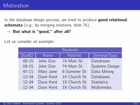
In the database design process, we tried to produce good relational

schemata (e.g., by merging relations, slide 76).

→ But what is “good,” after all?

Let us consider an example:

Students

StudID Name Address SeminarTopic

08-15 John Doe 74 Main St Databases

08-15 John Doe 74 Main St Systems Design

47-11 Mary Jane 8 Summer St Data Mining

12-34 Dave Kent 19 Church St Databases

12-34 Dave Kent 19 Church St Statistics

12-34 Dave Kent 19 Church St Multimedia


Update Anomalies

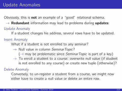
Obviously, this is not an example of a “good” relational schema.

→ Redundant information may lead to problems during updates:

Update Anomaly

If a student changes his address, several rows have to be updated.

Insert Anomaly

What if a student is not enrolled to any seminar?

→ Null value in column SeminarTopic?

(→ may be problematic since SeminarTopic is part of a key)

→ To enroll a student to a course: overwrite null value (if student

is not enrolled to any course) or create new tuple (otherwise)?

Delete Anomaly

Conversely, to un-register a student from a course, we might now

either have to create a null value or delete an entire row.


Decomposed Schema

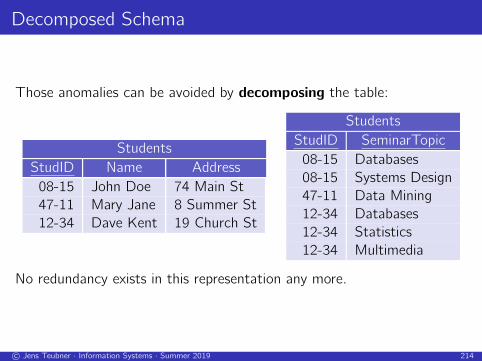
Those anomalies can be avoided by decomposing the table:

Students

StudID Name Address

08-15 John Doe 74 Main St

47-11 Mary Jane 8 Summer St

12-34 Dave Kent 19 Church St

Students

StudID SeminarTopic

08-15 Databases

08-15 Systems Design

47-11 Data Mining

12-34 Databases

12-34 Statistics

12-34 Multimedia

No redundancy exists in this representation any more.


Anomalies: Another Example

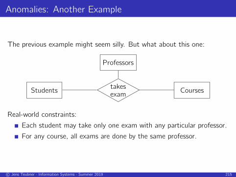
The previous example might seem silly. But what about this one:

Professors

Students Coursestakesexam

Real-world constraints:

Each student may take only one exam with any particular professor.

For any course, all exams are done by the same professor.


Anomalies: Another Example

Ternary relationship set → ternary relation:

TakesExam

Student Professor Course

John Doe Prof. Smart Information Systems

Dave Kent Prof. Smart Information Systems

John Doe Prof. Clever Computer Architecture

Mary Jane Prof. Bright Software Engineering

John Doe Prof. Bright Software Engineering

Dave Kent Prof. Bright Software Engineering

The association Course → Professor occurs multiple times.

Decomposition without that redundancy?


Functional Dependencies

Both examples contained instance of functional dependencies, e.g.,

Course → Professor .

We say that

“Course (functionally) determines Professor .”

meaning that when two tuples t1 and t2 agree on their Course values,

they must also contain the same Professor value.


Notation

For this chapter, we’ll simplify our notation a bit.

We use single capital letters A, B, C , . . . for attribute names.

We use a short-hand notation for sets of attributes:

ABCdef= {A,B,C} .

A functional dependency (FD) A1 . . .An → B1 . . .Bm on a relation

schema sch(R) describes a constraint that, for every instance R:

t.A1 = s.A1 ∧ · · · ∧ t.An = s.An ⇒ t.B1 = s.B1 ∧ · · · ∧ t.Bm = s.Bm .

→ A functional dependency is a constraint over one relation.

A1, . . . ,An,B1, . . . ,Bm must all be in sch(R).


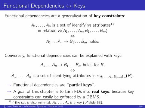
Functional Dependencies ↔ Keys

Functional dependencies are a generalization of key constraints:

A1, . . . ,An is a set of identifying attributes11

in relation R(A1, . . . ,An,B1, . . . ,Bm).⇔

A1 . . .An → B1 . . .Bm holds.

Conversely, functional dependencies can be explained with keys.

A1 . . .An → B1 . . .Bm holds for R.

⇔A1, . . . ,An is a set of identifying attributes in πA1,...,An,B1,...Bm(R).

→ Functional dependencies are “partial keys”.

→ A goal of this chapter is to turn FDs into real keys, because key

constraints can easily be enforced by a DBMS.11If the set is also minimal, A1, . . . ,An is a key (↗ slide 53).


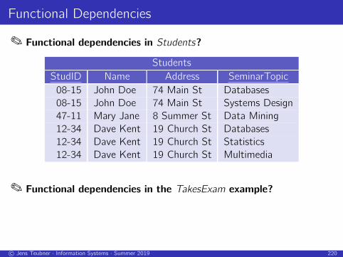
Functional Dependencies

� Functional dependencies in Students?

Students


08-15 John Doe 74 Main St Databases

08-15 John Doe 74 Main St Systems Design

47-11 Mary Jane 8 Summer St Data Mining

12-34 Dave Kent 19 Church St Databases

12-34 Dave Kent 19 Church St Statistics

12-34 Dave Kent 19 Church St Multimedia

� Functional dependencies in the TakesExam example?


Functional Dependencies, Entailment

A functional dependency with m attributes on the right-hand side

A1 . . .An → B1 . . .Bm

is equivalent to the m functional dependencies

A1 . . .An → B1...

...

A1 . . .An → Bm

Often, functional dependencies imply one another.

→ We say that a set of FDs F entails another FD f if the FDs in Fguarantee that f holds as well.

→ If a set of FDs F1 entails all FDs in the set F2, we say that F1 is a

cover of F2; F1 covers (all FDs in) F2.


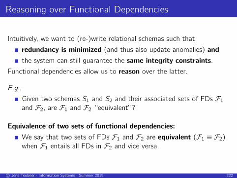
Reasoning over Functional Dependencies

Intuitively, we want to (re-)write relational schemas such that

redundancy is minimized (and thus also update anomalies) and

the system can still guarantee the same integrity constraints.

Functional dependencies allow us to reason over the latter.

E.g.,

Given two schemas S1 and S2 and their associated sets of FDs F1and F2, are F1 and F2 “equivalent”?

Equivalence of two sets of functional dependencies:

We say that two sets of FDs F1 and F2 are equivalent (F1 ≡ F2)when F1 entails all FDs in F2 and vice versa.


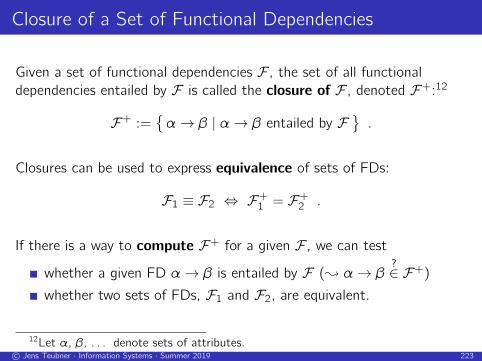
Closure of a Set of Functional Dependencies

Given a set of functional dependencies F , the set of all functional

dependencies entailed by F is called the closure of F , denoted F+:12

F+ :={α→ β | α→ β entailed by F

}.

Closures can be used to express equivalence of sets of FDs:

F1 ≡ F2 ⇔ F+1 = F+

2 .

If there is a way to compute F+ for a given F , we can test

whether a given FD α→ β is entailed by F (; α→ β?∈ F+)

whether two sets of FDs, F1 and F2, are equivalent.

12Let α, β, . . . denote sets of attributes.c© Jens Teubner · Information Systems · Summer 2019 223

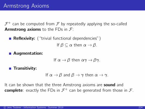
Armstrong Axioms

F+ can be computed from F by repeatedly applying the so-called

Armstrong axioms to the FDs in F :

Reflexivity: (“trivial functional dependencies”)

If β ⊆ α then α→ β.

Augmentation:

If α→ β then αγ → βγ.

Transitivity:

If α→ β and β → γ then α→ γ.

It can be shown that the three Amstrong axioms are sound and

complete: exactly the FDs in F+ can be generated from those in F .


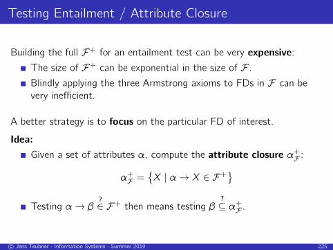
Testing Entailment / Attribute Closure

Building the full F+ for an entailment test can be very expensive:

The size of F+ can be exponential in the size of F .

Blindly applying the three Armstrong axioms to FDs in F can be

very inefficient.

A better strategy is to focus on the particular FD of interest.

Idea:

Given a set of attributes α, compute the attribute closure α+F :

α+F =

{X | α→ X ∈ F+

}Testing α→ β

?∈ F+ then means testing β

?⊆ α+

F .


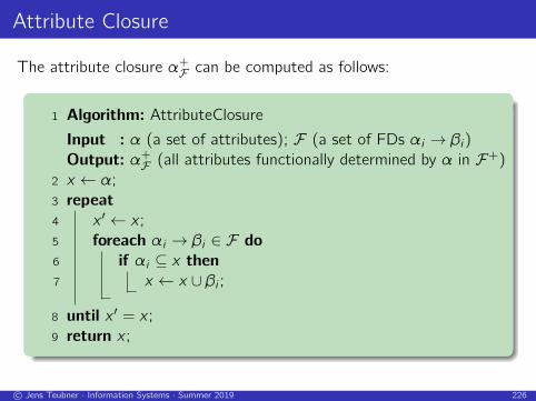
Attribute Closure

The attribute closure α+F can be computed as follows:

1 Algorithm: AttributeClosure

Input : α (a set of attributes); F (a set of FDs αi → βi)

Output: α+F (all attributes functionally determined by α in F+)

2 x ← α;

3 repeat

4 x ′ ← x ;

5 foreach αi → βi ∈ F do

6 if αi ⊆ x then

7 x ← x ∪ βi ;

8 until x ′ = x ;

9 return x ;


Example

Given

F = {AB → C ,D → E ,AE → G ,GD → H, ID → J}

for a relation R, sch(R) = ABCDEFGHIJ.

� ABD → GH entailed by F?

� ABD → HJ entailed by F?


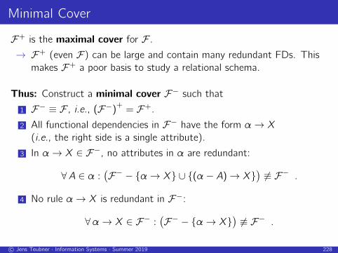
Minimal Cover

F+ is the maximal cover for F .

→ F+ (even F) can be large and contain many redundant FDs. This

makes F+ a poor basis to study a relational schema.

Thus: Construct a minimal cover F− such that

1 F− ≡ F , i.e., (F−)+ = F+.

2 All functional dependencies in F− have the form α→ X(i.e., the right side is a single attribute).

3 In α→ X ∈ F−, no attributes in α are redundant:

∀A ∈ α :(F− − {α→ X} ∪ {(α− A)→ X}

)6≡ F− .

4 No rule α→ X is redundant in F−:

∀α→ X ∈ F− :(F− − {α→ X}

)6≡ F− .


Constructing a Minimal Cover

To construct the minimal cover F−:

1 F− ← F where all functional dependencies are converted to have

only one attribute on the right side.

2 Remove redundant attributes from the left-hand sides of

functional dependencies in F−:

1 foreach α→ X ∈ F− do

2 foreach A ∈ α do

3 if X ∈ (α− A)+F− then A redundant in α? Remove

it.

4 F− ← F− − {α→ X} ∪ {(α− A)→ X};

3 Remove redundant functional dependencies from F−:

1 foreach α→ X ∈ F− do

2 if (F− − {α→ X}) ≡ F− then

3 F− ← F− − {α→ X} ;


Constructing a Minimal Cover

� Minimal cover for the following FDs?

ABH → C F → AD C → E E → FA→ D BGH → F BH → E

1 make right-hand sides atomic:ABH → C F → A F → D C → EE → F A→ D BGH → F BH → E

2 remove redundant attributes from left-hand sides:BH → C F → A F → D C → EE → F A→ D BH → F BH → E

3 remove redundant rules:BH → C F → A C → E E → FA→ D


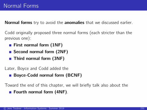
Normal Forms

Normal forms try to avoid the anomalies that we discussed earlier.

Codd originally proposed three normal forms (each stricter than the

previous one):

First normal form (1NF)

Second normal form (2NF)

Third normal form (3NF)

Later, Boyce and Codd added the

Boyce-Codd normal form (BCNF)

Toward the end of this chapter, we will briefly talk also about the

Fourth normal form (4NF).


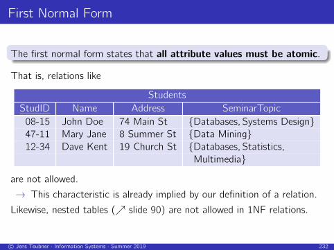
First Normal Form

The first normal form states that all attribute values must be atomic.

That is, relations like

Students


08-15 John Doe 74 Main St {Databases,Systems Design}47-11 Mary Jane 8 Summer St {Data Mining}12-34 Dave Kent 19 Church St {Databases,Statistics,

Multimedia}

are not allowed.

→ This characteristic is already implied by our definition of a relation.

Likewise, nested tables (↗ slide 90) are not allowed in 1NF relations.


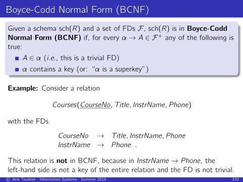
Boyce-Codd Normal Form (BCNF)

Given a schema sch(R) and a set of FDs F , sch(R) is in Boyce-Codd

Normal Form (BCNF) if, for every α→ A ∈ F+ any of the following is

true:

A ∈ α (i.e., this is a trivial FD)

α contains a key (or: “α is a superkey”)

Example: Consider a relation

Courses(CourseNo,Title, InstrName,Phone)

with the FDs

CourseNo → Title, InstrName,Phone

InstrName → Phone .

This relation is not in BCNF, because in InstrName → Phone, the

left-hand side is not a key of the entire relation and the FD is not trivial.c© Jens Teubner · Information Systems · Summer 2019 233

Boyce-Codd Normal Form (BCNF)

A BCNF schema can have more than one key. E.g.,

sch(R) = ABCD,

F = {AB → CD,AC → BD}.This relation is in BCNF, because the left-hand side of each of the two

FDs in F is a key.

BCNF prevents all of the anomalies that we saw earlier in this chapter.

→ By ensuring BCNF in our database designs, we can produce “good”

relational schemas.

A beauty of BCNF is that its FDs can easily be checked by a database

system.

→ Only need to mark left-hand sides as key in the relational schema.


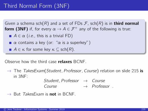
Third Normal Form (3NF)

Given a schema sch(R) and a set of FDs F , sch(R) is in third normal

form (3NF) if, for every α→ A ∈ F+ any of the following is true:

A ∈ α (i.e., this is a trivial FD)

α contains a key (or: “α is a superkey”)

A ∈ κ for some key κ ⊆ sch(R).

Observe how the third case relaxes BCNF.

→ The TakesExam(Student,Professor ,Course) relation on slide 215 is

in 3NF:Student,Professor → Course

Course → Professor .

→ But TakesExam is not in BCNF.


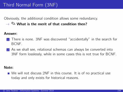
Third Normal Form (3NF)

Obviously, the additional condition allows some redundancy.

→ � What is the merit of that condition then?

Answer:

1 There is none. 3NF was discovered “accidentally” in the search for

BCNF.

2 As we shall see, relational schemas can always be converted into

3NF form losslessly, while in some cases this is not true for BCNF.

Note:

We will not discuss 2NF in this course. It is of no practical use

today and only exists for historical reasons.


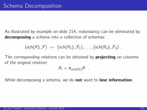
Schema Decomposition

As illustrated by example on slide 214, redundancy can be eliminated by

decomposing a schema into a collection of schemas:(sch(R),F

);

(sch(R1),F1

), . . . ,

(sch(Rn),Fn

).

The corresponding relations can be obtained by projecting on columns

of the original relation:

Ri = πsch(Ri )R .

While decomposing a schema, we do not want to lose information.


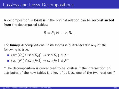
Lossless and Lossy Decompositions

A decomposition is lossless if the original relation can be reconstructed

from the decomposed tables:

R = R1 1 · · · 1 Rn .

For binary decompositions, losslessness is guaranteed if any of the

following is true:(sch(R1) ∩ sch(R2)

)→ sch(R1) ∈ F+(

sch(R1) ∩ sch(R2))→ sch(R2) ∈ F+

“The decomposition is guaranteed to be lossless if the intersection of

attributes of the new tables is a key of at least one of the two relations.”


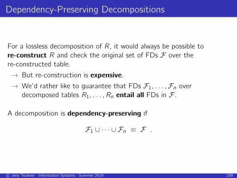
Dependency-Preserving Decompositions

For a lossless decomposition of R, it would always be possible to

re-construct R and check the original set of FDs F over the

re-constructed table.

→ But re-construction is expensive.

→ We’d rather like to guarantee that FDs F1, . . . ,Fn over

decomposed tables R1, . . . ,Rn entail all FDs in F .

A decomposition is dependency-preserving if

F1 ∪ · · · ∪ Fn ≡ F .


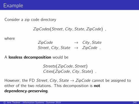
Example

Consider a zip code directory

ZipCodes(Street,City ,State,ZipCode) ,

whereZipCode → City ,State

Street,City ,State → ZipCode .

A lossless decomposition would be

Streets(ZipCode,Street)Cities(ZipCode,City ,State) .

However, the FD Street,City ,State → ZipCode cannot be assigned to

either of the two relations. This decomposition is not

dependency-preserving.


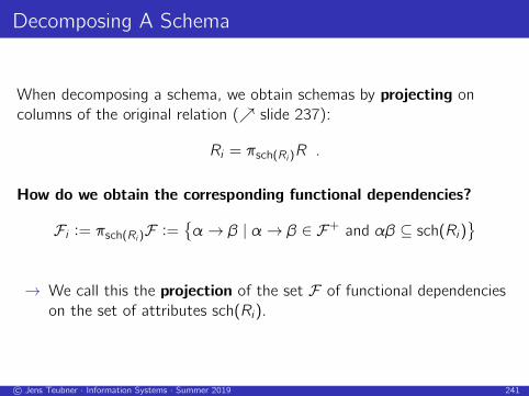
Decomposing A Schema

When decomposing a schema, we obtain schemas by projecting on

columns of the original relation (↗ slide 237):

Ri = πsch(Ri )R .

How do we obtain the corresponding functional dependencies?

Fi := πsch(Ri )F :={α→ β | α→ β ∈ F+ and αβ ⊆ sch(Ri)

}→ We call this the projection of the set F of functional dependencies

on the set of attributes sch(Ri).


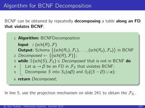
Algorithm for BCNF Decomposition

BCNF can be obtained by repeatedly decomposing a table along an FD

that violates BCNF:

1 Algorithm: BCNFDecomposition

Input : (sch(R),F)Output: Schema

{(sch(R1),F1), . . . , (sch(Rn),Fn)

}in BCNF

2 Decomposed ←{(sch(R),F)

};

3 while ∃ (sch(S),FS) ∈ Decomposed that is not in BCNF do

4 Let α→ β be an FD in FS that violates BCNF;

5 Decompose S into S1(αβ) and S2((S − β) ∪ α);6 return Decomposed ;

In line 5, use the projection mechanism on slide 241 to obtain the FSi .


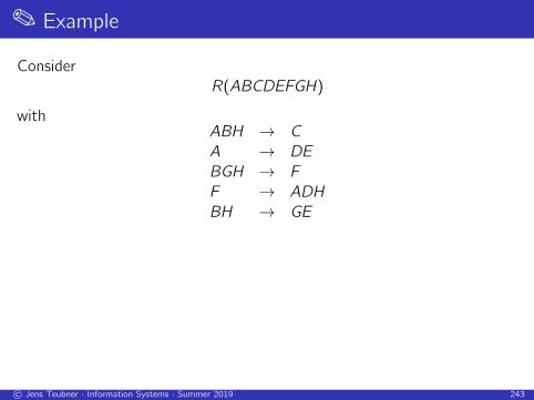
� Example

Consider

R(ABCDEFGH)

withABH → C

A → DE

BGH → F

F → ADH

BH → GE


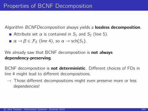
Properties of BCNF Decomposition

Algorithm BCNFDecomposition always yields a lossless decomposition.

Attribute set α is contained in S1 and S2 (line 5).

α→ β ∈ FS (line 4), so α→ sch(S1).

We already saw that BCNF decomposition is not always

dependency-preserving.

BCNF decomposition is not deterministic. Different choices of FDs in

line 4 might lead to different decompositions.

→ Those different decompositions might even preserve more or less

dependencies!


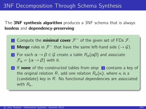
3NF Decomposition Through Schema Synthesis

The 3NF synthesis algorithm produces a 3NF schema that is always

lossless and dependency-preserving:

1 Compute the minimal cover F− of the given set of FDs F .

2 Merge rules in F− that have the same left-hand side (→ G).

3 For each α→ β ∈ G create a table Rα(αβ) and associate

Fα = {α→ β} with it.

4 If none of the constructed tables from step 3 contains a key of

the original relation R, add one relation Rκ(κ), where κ is a

(candidate) key in R. No functional dependencies are associated

with Rκ.


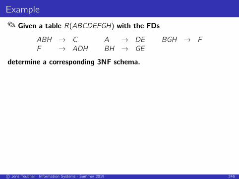
Example

� Given a table R(ABCDEFGH) with the FDs

ABH → C A → DE BGH → F

F → ADH BH → GE

determine a corresponding 3NF schema.

1 Compute the minimal cover:

1 Make right-hand sides atomic:

ABH → C A → D A → E

BGH → F F → A F → D

F → H BH → G BH → E

2 Remove redundant attributes (left-hand side):

BH → C A → D A → E

BH → F F → A F → D

F → H BH → G BH → E


Example (cont.)

1 minimal cover (cont.):

3 Remove redundant rules:

BH → C A → D A → E

BH → F F → A

F → H BH → G

2 Merge functional dependencies in F−:

BH → CFG A → DE F → AH .

3 Create a table for each FD:

R1(BHCFG ) R2(ADE ) R3(FAH)

4 Any Ri contains a key of R?

→ Yes. (BH → F ; F → A; all attributes of R are in R1,R2,R3)

→ We are done.


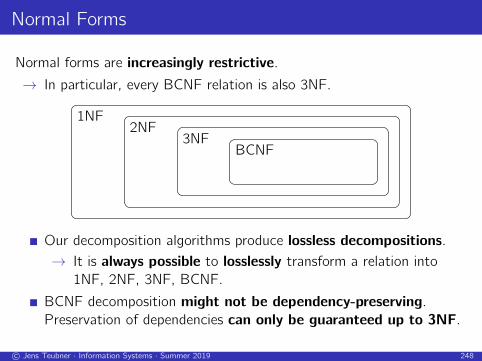
Normal Forms

Normal forms are increasingly restrictive.

→ In particular, every BCNF relation is also 3NF.

1NF2NF

3NFBCNF

Our decomposition algorithms produce lossless decompositions.

→ It is always possible to losslessly transform a relation into

1NF, 2NF, 3NF, BCNF.

BCNF decomposition might not be dependency-preserving.

Preservation of dependencies can only be guaranteed up to 3NF.


BCNF vs. 3NF

BCNF decomposition is non-deterministic.

→ Some decompositions might be dependency-preserving, some

might not.

Decomposition strategy:

1 Establish 3NF schema (through synthesis; dependency preservation

guaranteed).

2 Decompose resulting schema to obtain BCNF.

→ This strategy typically leads to “good” (dependency-preserving if

possible) BCNF decompositions.


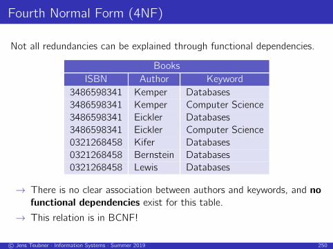
Fourth Normal Form (4NF)

Not all redundancies can be explained through functional dependencies.

Books

ISBN Author Keyword

3486598341 Kemper Databases

3486598341 Kemper Computer Science

3486598341 Eickler Databases

3486598341 Eickler Computer Science

0321268458 Kifer Databases

0321268458 Bernstein Databases

0321268458 Lewis Databases

→ There is no clear association between authors and keywords, and no

functional dependencies exist for this table.

→ This relation is in BCNF!


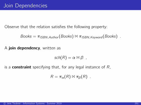
Join Dependencies

Observe that the relation satisfies the following property:

Books = πISBN,Author (Books) 1 πISBN,Keyword(Books) .

A join dependency, written as

sch(R) = α 1 β ,

is a constraint specifying that, for any legal instance of R,

R = πα(R) 1 πβ(R) .


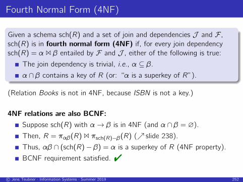
Fourth Normal Form (4NF)

Given a schema sch(R) and a set of join and dependencies J and F ,

sch(R) is in fourth normal form (4NF) if, for every join dependency

sch(R) = α 1 β entailed by F and J , either of the following is true:

The join dependency is trivial, i.e., α ⊆ β.

α ∩ β contains a key of R (or: “α is a superkey of R”).

(Relation Books is not in 4NF, because ISBN is not a key.)

4NF relations are also BCNF:

Suppose sch(R) with α→ β is in 4NF (and α ∩ β = ∅).

Then, R = παβ(R) 1 πsch(R)−β(R) (↗ slide 238).

Thus, αβ ∩ (sch(R)− β) = α is a superkey of R (4NF property).

BCNF requirement satisfied. "


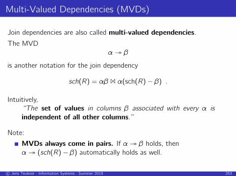
Multi-Valued Dependencies (MVDs)

Join dependencies are also called multi-valued dependencies.

The MVD

α� β

is another notation for the join dependency

sch(R) = αβ 1 α(sch(R)− β) .

Intuitively,

“The set of values in columns β associated with every α is

independent of all other columns.”

Note:

MVDs always come in pairs. If α� β holds, then

α� (sch(R)− β) automatically holds as well.


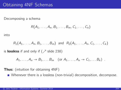
Obtaining 4NF Schemas

Decomposing a schema

R(A1, . . . ,An,B1, . . . ,Bm,C1, . . . ,Ck)

into

R1(A1, . . . ,An,B1, . . . ,Bm) and R2(A1, . . . ,An,C1, . . . ,Ck)

is lossless if and only if (↗ slide 238)

A1, . . . ,An � B1, . . .Bm (or A1, . . . ,An � C1, . . .Bk) .

Thus: (intuition for obtaining 4NF)

Whenever there is a lossless (non-trivial) decomposition, decompose.


Documents

Information Systems (Informationssysteme)dbis.cs.tu-dortmund.de/cms/de/lehre/ss19/infosys/slides/normalization.pdf · Motivation In the database design process, we tried to produce