Embed Size (px)
Citation preview

Title Page
Dual Purpose Bridge Health Monitoring and Weigh-in-motion (BWIM)
Phase I
FINAL REPORT
Richard Christenson and Sarira Motaref
Report Number
CT-2265-F-15-7
SPR-2265
Submitted to the
Connecticut Department of Transportation
Bureau of Policy and Planning
Roadway Information Systems Research Section
Michael Connors
Assistant Planning Director
July 7, 2016
Department of Civil and Environmental Engineering
School of Engineering
University of Connecticut

ii
FINAL REPORT
Disclaimer
This report [article, paper or publication] does not constitute a standard, specification or
regulation. The contents of this report reflect the views of the authors who are responsible for
the facts and the accuracy of the data presented herein. The contents do not necessarily reflect
the views of the Connecticut Department of Transportation or the Federal Highway
Administration.

iii
FINAL REPORT
Acknowledgments
The authors would like to acknowledge the efforts of numerous Connecticut Department of
Transportation employees in particular Anne-Marie McDonnell and Paul Dattilio. The authors
would also like to acknowledge the efforts of Susan Bakulski who worked as a research assistant
at the University of Connecticut on this project.
This report was prepared by the University of Connecticut, in cooperation with the Connecticut
Department of Transportation and the United States Department of Transportation, Federal
Highway Administration. The opinions, findings and conclusions expressed in the publication
are those of the authors and not necessarily those of the Connecticut Department of
Transportation or the Federal Highway Administration. This publication is based upon publicly
supported research and is copyrighted. It may be reproduced in part or in full, but it is requested
that there be customary crediting of the source.

iv
FINAL REPORT
Standard Conversions
SI* (MODERN METRIC) CONVERSION FACTORS APPROXIMATE CONVERSIONS TO SI UNITS
Symbol When You Know Multiply By To Find Symbol
LENGTH in inches 25.4 millimeters mm ft feet 0.305 meters m yd yards 0.914 meters m mi miles 1.61 kilometers km
AREA in
2square inches 645.2 square millimeters mm
2
ft2
square feet 0.093 square meters m2
yd2
square yard 0.836 square meters m2
ac acres 0.405 hectares ha mi
2square miles 2.59 square kilometers km
2
VOLUME fl oz fluid ounces 29.57 milliliters mL
gal gallons 3.785 liters L ft
3 cubic feet 0.028 cubic meters m
3
yd3
cubic yards 0.765 cubic meters m3
NOTE: volumes greater than 1000 L shall be shown in m3
MASS oz ounces 28.35 grams g
lb pounds 0.454 kilograms kgT short tons (2000 lb) 0.907 megagrams (or "metric ton") Mg (or "t")
TEMPERATURE (exact degrees) oF Fahrenheit 5 (F-32)/9 Celsius
oC
or (F-32)/1.8
ILLUMINATION fc foot-candles 10.76 lux lx fl foot-Lamberts 3.426 candela/m
2 cd/m
2
FORCE and PRESSURE or STRESS lbf poundforce 4.45 newtons N lbf/in
2poundforce per square inch 6.89 kilopascals kPa
APPROXIMATE CONVERSIONS FROM SI UNITS
Symbol When You Know Multiply By To Find Symbol
LENGTHmm millimeters 0.039 inches in m meters 3.28 feet ft m meters 1.09 yards yd
km kilometers 0.621 miles mi
AREA mm
2 square millimeters 0.0016 square inches in
2
m2 square meters 10.764 square feet ft
2
m2 square meters 1.195 square yards yd
2
ha hectares 2.47 acres ac km
2 square kilometers 0.386 square miles mi
2
VOLUME mL milliliters 0.034 fluid ounces fl oz
L liters 0.264 gallons gal
m3
cubic meters 35.314 cubic feet ft3
m3
cubic meters 1.307 cubic yards yd3
MASS g grams 0.035 ounces ozkg kilograms 2.202 pounds lbMg (or "t") megagrams (or "metric ton") 1.103 short tons (2000 lb) T
TEMPERATURE (exact degrees) oC Celsius 1.8C+32 Fahrenheit
oF
ILLUMINATION lx lux 0.0929 foot-candles fc cd/m
2candela/m
20.2919 foot-Lamberts fl
FORCE and PRESSURE or STRESS N newtons 0.225 poundforce lbf
kPa kilopascals 0.145 poundforce per square inch lbf/in2
*SI is the symbol for th International System of Units. Appropriate rounding should be made to comply with Section 4 of ASTM E380. e
(Revised March 2003)

v
FINAL REPORT
Technical Report Documentation Page
1. Report No. CT-2265-F-15-7
2. Government Accession No.
3. Recipient’s Catalog No.
4. Title and Subtitle Dual Purpose Bridge Health Monitoring and Weigh-in-motion (BWIM) Phase I
5. Report Date July 7, 2016
6. Performing Organization Code
7. Author(s) Richard Christenson and Sarira Motaref
8. Performing Organization Report No.
9. Performing Organization Name and Address University of Connecticut Connecticut Transportation Institute 270 Middle Turnpike, U-5202 Storrs, Connecticut 06269-5202
10 Work Unit No. (TRIS) N/A
11. Contract or Grant No. N/A
13. Type of Report and Period Covered Final Report August 1, 2009 – June 30, 2011
12. Sponsoring Agency Name and Address Connecticut Department of Transportation 2800 Berlin Turnpike Newington, CT 06131-7546
14. Sponsoring Agency Code SPR-2265
15. Supplementary Notes Prepared in cooperation with the U.S. Department of Transportation, Federal Highway
Administration, Connecticut Department of Transportation
16. Abstract The dual-purpose bridge health monitoring (BHM) and bridge weigh-in-motion (BWIM) system proposed in this research project establishes a single monitoring system, comprised of sensors, data acquisition, and processing, to provide both long-term health monitoring of a highway bridge and bridge-weigh-in-motion capabilities. A prototype dual-purpose BHM/BWIM system is presented that has been designed to examine the challenges associated with implementing a combined BHM/BWIM bridge monitoring system. This prototype system is currently being deployed in Connecticut on Interstate 91 (I-91) northbound in the town of Meriden, Connecticut. The BHM/BWIM design and initial results are provided in this report.
17. Key Words Bridge Monitoring, Weigh-in-motion,
BWIM, Bridge Structural Health, Bridge Inspection, Vibration Sensors
18.Distribution Statement No restrictions. This document is available to the
public through the National Technical Information Service, Springfield, Virginia 22161. The report is available on-line from National Transportation Library at http://ntl.bts.gov.
19. Security Classif. (of report) Unclassified
20. Security Classif. (of this page) Unclassified
21. No. of Pages 58
21. Price
Form DOT F 1700.7 (8-72) Reproduction of completed page authorized

vi
FINAL REPORT
Table of Contents
1-INTRODUCTION .................................................................................................................................................. 1
2-LITERATURE REVIEW ...................................................................................................................................... 5 2-1- Bridge Weigh-In-Motion (BWIM) ................................................................................................................................ 5 2-2- Bridge Health Monitoring (BHM) ................................................................................................................................ 5
3-INSTRUMENTATION AND INSTALLATION ................................................................................................ 6 3.1 Sensors and Recording Tools ............................................................................................................................................ 6
3-1-1-Foil Strain Gages ............................................................................................................................................... 7 3-1-2-Piezoelectric Strain Gages............................................................................................................................. 9 3-1-3-Piezoelectric Accelerometers .................................................................................................................... 11 3-1-4-Capacitance Accelerometers...................................................................................................................... 13 3-1-5-Resistance Temperature Detectors ........................................................................................................ 14 3-1-6-Microphone ....................................................................................................................................................... 15 3-1-7-Video Camera ................................................................................................................................................... 16
3-2-System Components .......................................................................................................................................................... 17 3-2-1-Computer ........................................................................................................................................................... 17 3-2-2-Data Acquisition Unit .................................................................................................................................... 18 3-2-3-Data Acquisition Hardware ........................................................................................................................ 19 3-2-4-Data Acquisition Modules ........................................................................................................................... 20 3-2-5-USB Mobile Broadband ................................................................................................................................ 24 3-2-6-Digi Connect WAN 3G modem .................................................................................................................. 24
3-3-Sensor Connections to System Components .......................................................................................................... 25 3-3-1-Foil Strain Gage Connection to System .................................................................................................. 25 3-3-2-Piezoelectric Strain Gage ............................................................................................................................. 26 3-3-3-Piezoelectric Accelerometer ...................................................................................................................... 27 3-3-4-Capacitance Accelerometer ........................................................................................................................ 27 3-3-5-Resistance Temperature Detector .......................................................................................................... 29
4-BWIM ................................................................................................................................................................... 29 4-1-BWIM methodology .......................................................................................................................................................... 29 4-2-Field study ............................................................................................................................................................................. 33
4-2-1-Truck of known weight ................................................................................................................................ 34 4-3-Test results and evaluation ........................................................................................................................................... 34
5-BHM ..................................................................................................................................................................... 39 5-1-BHM methodology ............................................................................................................................................................. 39 5-2- Probabilistic approach ................................................................................................................................................... 42 5-3-Accounting for thermal and truck weight effects in BHM .............................................................................. 43
REFERENCES ......................................................................................................................................................... 46

vii
FINAL REPORT
List of Tables
Table 1- Comparison of Measured and Calculated Truck Speed ....................................................................... 35
Table 2- Comparison of measured and calculated truck axle spacing ............................................................ 38
Table 3- Comparison of measured (68,600-lb (3116-kg)) to calculated truck weight ............................ 39
List of Figures
Figure 1: Installation of the dual BHM/BWIM system on the Meriden Bridge. ............................................ 3
Figure 2: Schematic of sensors layout and sensors type for the Meriden Bridge ........................................ 6
Figure 3: Foil strain gages used on the Meriden Bridge .......................................................................................... 7
Figure 4: Foil Strain Sensor Layout (Plan View) ......................................................................................................... 9
Figure 5: Piezoelectric strain sensors ............................................................................................................................. 9
Figure 6: Plan view of piezoelectric strain sensors layout ................................................................................... 10
Figure 7: Piezoelectric accelerometer sensors .......................................................................................................... 11
Figure 8: Plan view of piezoelectric accelerometer sensors layout ................................................................. 12
Figure 9: Piezoelectric accelerometer sensors with frequency range of 0.15 to 1000 Hz (picture from vendor) ........................................................................................................................................................................... 13
Figure 10: K-Beam Variable capacitance accelerometer ...................................................................................... 13
Figure 11: Plan view of capacitance accelerometer sensor layout ................................................................... 14
Figure 12: Plan view of resistance temperature detectors layout .................................................................... 15
Figure 13: Resistance temperature detector sensor ............................................................................................... 15
Figure 14: Microphone to measure global vibration of bridge ........................................................................... 16
Figure 15: Video Camera to capture image of vehicles (picture from vendor) ........................................... 17
Figure 16: Computer for data acquisition at Meriden Bridge ............................................................................. 17
Figure 17: Cabinet housing system components under Meriden Bridge ....................................................... 18
Figure 18: NI cDAQ-9178 CompactDAQ Chassis ...................................................................................................... 19
Figure 19: Data acquisition modules ............................................................................................................................. 20
Figure 20: NI 9236 module for collection of foil Strain gages data .................................................................. 20
Figure 21: NI 9234 module for collection of piezoelectric accelerometers/strain gages data ............. 21
Figure 22: NI 9206 module for collection of capacitance accelerometer data............................................. 22
Figure 23: NI 9217 for collection of temperature sensors data ......................................................................... 22
Figure 24: NI 9232 for collection of piezoelectric strain gages data (picture from vendor) ................. 23
Figure 25: USB mobile modem (picture from vendor) .......................................................................................... 24
Figure 26: Digi Connect WAN 3G modem (picture from vendor) ..................................................................... 25

viii
FINAL REPORT
Figure 27: An installed foil strain gage on the Meriden Bridge .......................................................................... 25
Figure 28: Magnetic mount to install piezoelectric strain sensors ................................................................... 26
Figure 29: A power supply to power the capacitance accelerometers (picture from vendor) ............. 28
Figure 30: An installed resistance temperature detector on the Meriden Bridge ...................................... 29
Figure 31: Truck of known weight ................................................................................................................................. 34
Figure 32: Piezoelectric accelerometer vs. capacitive accelerometer data: (a) time history for truck crossing; (b) auto power spectral density of acceleration. .................................................................................. 36
Figure 33: Piezoelectric strain sensors vs. foil Strain gages data: (a) time history for truck crossing; (b) autopower spectral density of acceleration. ....................................................................................................... 37
Figure 34: Negative spikes in second derivative of strain measurement when the truck axles pass over the mid-span of the bridge ...................................................................................................................................... 38

ix
FINAL REPORT
Executive Summary
The dual-purpose bridge health monitoring (BHM) and bridge weigh-in-motion (BWIM)
system proposed in this research project establishes a single monitoring system, comprised of
sensors, data acquisition, and processing, to provide both long-term health monitoring of a
highway bridge and bridge-weigh-in-motion capabilities. A prototype dual-purpose
BHM/BWIM system is presented that has been designed to examine the challenges associated
with implementing a combined BHM/BWIM bridge monitoring system. This prototype system
is currently being deployed in Connecticut on Interstate 91 (I-91) northbound in the town of
Meriden, Connecticut. The BHM/BWIM design and initial results are provided in this report.

1
1-INTRODUCTION
The dual-purpose bridge health monitoring and weigh-in-motion system proposed
in this research project establishes a single monitoring system, comprised of sensors, data
acquisition, and processing, to provide both long-term health monitoring of a highway
bridge and bridge-weigh-in-motion capabilities. The goal of long-term bridge monitoring
is to identify changes in a bridge’s dynamic behavior over multi-year periods as an
indicator of the structural health of the bridge. To achieve this goal, highway bridges are
instrumented with sensors, data acquisition and processing power. Vibration-based
health monitoring shows great promise to supplement bridge inspections and provide
bridge owners with timely information on the structural condition of the bridge
infrastructure. The premise of vibration-based monitoring is that damage or a change in
the structure will result in a corresponding change in the stiffness (or mass) of the
structure, which will change the structure’s dynamic characteristics and ultimately the
response to a dynamic loading.
Transportation agencies are faced with the need to design and improve
transportation networks to meet the ever increasing demand for safe, efficient and cost
effective transport of people and goods. To meet this need, whether for the design of
infrastructure (bridges and pavements), application of air quality or freight models, or
enforcement of the size and weight limits, information is needed to quantify the loads
experienced on the network. Weight data and related traffic data are used for a variety of
engineering designs and decisions. Weigh-in-motion (WIM) systems are one mechanism
used to gather such weight data. WIM systems present many challenges to employ,

2
including cost, installation, calibration, maintenance and accuracy. Alternative means to
collect weight data, in particular non-intrusive methods, are desired.
Bridge Weigh-In-Motion (BWIM) uses the dynamic response of a bridge to
determine gross weight, speed, and axle spacing of vehicles. The advantage of BWIM is
that it does not require installation of sensors in the pavement, nor use any axle detectors
in the roadway. To date, studies have all been short-term applications of BWIM. A
recent study by the Connecticut Academy of Science and Engineering (CASE)
recommends that BWIM, as a promising non-intrusive technology, should be considered
for WIM in Connecticut (CASE, 2008).
Bridge WIM systems and bridge health monitoring (BHM) systems, which use
structural response measurements to identify the structural condition of the bridge, have
similar components. By considering this leveraged BHM/BWIM application, more
comprehensive data can be collected. Augmenting long-term bridge monitoring systems
with BWIM will enable agencies to collect weight data on a more comprehensive
network. Improved load information on the transportation network will lead to better
bridge, pavement and highway designs, as well as improved decisions and efficiency; the
ability to weigh and screen commercial vehicles in a timely fashion for weight
enforcement; the collection of speed, weight and class data for traffic monitoring; and
increased safety and timely identification of changes in the structural system for
maintenance and operation. The actual measured volume and speed of traffic combined
with indicators of structural degradation can also benefit planning, if implemented at a
system level. Truck traffic attributes that are important for weight enforcement,

3
structural health monitoring, and traffic monitoring can be determined and shared through
the use of combined BHM/BWIM systems.
A prototype dual-purpose BHM/BWIM system is presented that has been
designed to examine the challenges associated with implementing a combined
BHM/BWIM bridge monitoring system. This prototype system is currently being
deployed in Connecticut on Interstate 91 (I-91) northbound in the town of Meriden,
Connecticut. The bridge is ideally located prior to an operational Connecticut static
weigh scale. This proximity will not only allow the project to validate BWIM
measurements with the static scale, but will facilitate assessment of how the results from
a leveraged BHM/BWIM system can benefit enforcement, bridge health monitoring and
traffic monitoring efforts at federal, state and local transportation agencies.
Figure 1: Installation of the dual BHM/BWIM system on the Meriden Bridge.

4
The test bridge is a simply-supported steel-girder bridge built in 1964 located on
I-91 over Baldwin Avenue in Meriden, Connecticut, and referred to herein as the
Meriden Bridge. Figure 1 shows a picture of the Bridge during installation of the
monitoring system. This single-span bridge is 85 feet in length with multiple plate-
stringers supported by eight girders. The bridge has less than a 12% skew and 3%
longitudinal slope. The bridge carries three lanes of Northbound traffic with an annual
average daily traffic (AADT) of 57,000 vehicles, comprised of 9% trucks.
The physical equipment of the BWIM/BHM system includes instrumentation for
an automatic data acquisition system to monitor dynamic beam strains and vertical
acceleration due to traffic loading as well as the corresponding surface temperature of the
bridge girders. Sensors measure physical responses (i.e. strain, acceleration and
temperature) into analog electrical signals; and the data acquisition system converts the
analog electrical signals of the sensors into digital signals. The output from the digital
signals is saved for archiving and further processing purposes. It is possible to configure
the system to compute real-time BHM and BWIM measurements, but for the purposes of
this research the signals are saved for specific research objectives including the analysis
of the sensor technologies for this application. Real-time computation of data in addition
to saving the signals would require significantly more processing capabilities. The
prototype BHM/BWIM system has been designed to meet specific research objectives
including flexibility in available measurements for further BHM and BWIM development
and evaluation of various sensor technologies for this application.

5
2-LITERATURE REVIEW
A brief literature review is provided in this section for both bridge weigh-in-
motion and bridge health monitoring.
2-1- Bridge Weigh-In-Motion (BWIM)
Proposed over 30 years ago by Moses (Moses, 1979), BWIM continues to receive
attention with the advancement of sensor and data acquisition technologies and with the
extensive research conducted in Europe in the 1990’s through the Weighing in motion of
Axles and Vehicles for Europe (WAVE) project (Jacob, 2002). BWIM uses sensing,
acquisition, and processing capabilities similar to those used in vibration-based BHM.
Recent work on BWIM in France, Slovenia and Ireland has focused on fully portable
temporary installations for enforcement and is typically limited to short single-span
bridges. To date BWIM has been used in India, Canada and throughout Europe. A
project to test and evaluate BWIM in the United States was recently conducted at the
University of Alabama using the portable BWIM system developed in Europe.
Additionally, the Connecticut Department of Transportation (CTDOT) and the University
of Connecticut (UConn) have completed pilot studies on BWIM, in 2006 and 2008,
which have focused on single-span steel-girder bridges (Cardini, A.J. and DeWolf, J.T.
2009; Wall C. and Christenson, R., 2009).
2-2- Bridge Health Monitoring (BHM)
Research is on-going in the area of long-term bridge monitoring, in particular
long-term vibration-based monitoring for the purposes of detecting damage, monitoring
deterioration and allocating resources (Farrar et al., 1999, Chakraborty et al., 1995,
Salawu et al., 1997, Doebling et al., 1996, Caicedo et al., 2000, and Chang, 2000).
Bridge Monitoring systems were specifically identified in the Federal SAFETEA-LU
6
Legislation [5202] (FHWA, 2005). The Connecticut Department of Transportation
(CTDOT) and University of Connecticut (UConn) have a long history of close
partnership in bridge monitoring, with over three decades of bridge health monitoring
(BHM) experience. Connecticut has experience with six permanently monitored bridges
that include a variety of bridge types including a post-tensioned segmental concrete box-
girder, multi-girder steel composite, curved steel box-girder, hung span in a large truss,
and continuous plate girder bridge (Olund et al., 2006, DeWolf et al., 2009, Scianna, et
al., 2014a, 2014b, 2014c, and 2014d, Plude et al., 2014, Prusaczyk et al., 2014, and
Christenson et al., 2014).
3-INSTRUMENTATION AND INSTALLATION
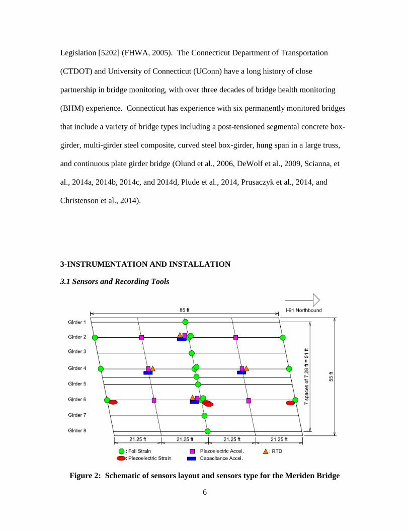
3.1 Sensors and Recording Tools
Figure 2: Schematic of sensors layout and sensors type for the Meriden Bridge

7
The Meriden Bridge has a dual-purpose BHM and BWIM system comprised of
strain sensors, accelerometers, and temperature detectors for 38 total sensors and 5
different sensing technologies. There are eighteen foil strain gages, 4 piezoelectric strain
sensors, 8 piezoelectric accelerometers, 4 capacitance accelerometers (with additional
temperature sensing capability), and 4 resistance temperature detectors (RTD). The
sensor layout and their types are shown in Figure 2.
3-1-1-Foil Strain Gages
Figure 3: Foil strain gages used on the Meriden Bridge
Foil strain sensors are commonly used for dynamic strain measurements in bridge
monitoring. These sensors have a large measurement range, typically 1000s of
microstrain (με). The bridge girders have been observed to have peak strains less than
100 με. Vishay Micro-Measurements manufactures the foil strain gages used for this
installation.
A total of eighteen quarter-bridge foil-strain gages are installed on the Meriden
Bridge. Figure 3 shows an image of the foil-strain gage prior to installation and Figure 4
provides a diagram of the sensor layout, as installed. Specifically:
Six foil-strain sensors are installed on the bearings at bridge abutments on
girders 2, 4, and 6. Bearings on girders 2, 4 and 6 were selected because
each is located directly under one of the three lanes of traffic, respectively.

8
It is anticipated that the sensors installed at these locations will be well
situated to detect vehicle loading on and off of the bridge and hence
capture the presence of vehicles on the bridge.
One foil strain gage is attached on the stringer in the middle of the bridge
at the midspan (location K). This sensor is intended to measure axial
strain in the stringer to identify if this stringer takes on any significant load
during normal vehicle loading.
Eleven foil strain gages are located at the midspan of steel girders 1
through 8 on the web, just above the bottom flange, and on girders 2, 4
and 6 on the web, just below the top flange. It is anticipated that the
largest strain measurements will be collected at the midspan. The larger
measurements provide a benefit of an improved signal-to-noise ratio.
Having strain sensors on each of the eight girders enables the calculation
of the strain distribution across the girders and also allows for strains
resulting from vehicles traveling in multiple lanes across the bridge to be
measured. Strain sensor measurements from the top and bottom of the
web allow for the determination of the neutral axis for that particular
cross-section. The location of the neutral axis is very important for bridge
health monitoring. Applications of the neutral axis for BHM include: 1)
the neutral axis is used in the assessment of the composite behavior of the
bridge girders with respect to the bridge deck; 2) detection of any changes
in the location of the neutral axis are indicative of deck damage.

9
Figure 4: Foil Strain Sensor Layout (Plan View)
3-1-2-Piezoelectric Strain Gages
Figure 5: Piezoelectric strain sensors
Four piezoelectric strain gages, also referred to as high sensitivity quartz strain
transducers, are installed on the Meriden Bridge (Fig. 5). All four sensors are located on
girder 6. This girder was selected because it is directly below the right travel lane. The
majority of the truck traffic travels in this right travel lane. There is one piezoelectric

10
strain gage at each bearing and two piezoelectric strain gages at the midspan, top and
bottom of the web. These sensors are collocated with the foil strain gages. Figure 6
shows the piezoelectric strain sensors layout.
Figure 6: Plan view of piezoelectric strain sensors layout
The piezoelectric strain sensors can provide more sensitive strain measurements
with a strain range of ±140 με and a bandwidth down to 0.004 Hz (a time constant of 113
seconds) for the configuration here. Use of this type of strain sensor to collect low
frequency dynamic measurements on a highway bridge is a new application. The sensors
are manufactured by the Kistler Instrument Corporation. Two additional components are
used to convert the piezoelectric signal to a voltage output. They are the impedance
converter (Model 558) and a range capacitor (Model 571A5), produced by National
Instruments Corporation. The nominal sensitivity of the piezoelectric strain sensor with
impedance converter and range capacitor is 35.430 mV/με. The use and layout of these
items will be further discussed in the section 3-3-2.

11
3-1-3-Piezoelectric Accelerometers
Figure 7: Piezoelectric accelerometer sensors
Eight integrated circuit piezoelectric accelerometers are installed on the test
bridge. Traditionally, accelerometers are used mainly in bridge health monitoring. This
dual-purpose system was designed to include accelerometers both for the traditional
bridge health monitoring measurements and for exploratory application and further

12
comparison to the bridge weigh-in-motion results from the strain gages.
Figure 8: Plan view of piezoelectric accelerometer sensors layout
Figure 7 shows an image of the piezoelectric accelerometer, manufactured by
PCB Piezotronics, Inc. The piezoelectric accelerometers have a ±0.25 g peak acceleration
level and a frequency range from 0.1 to 200 Hz. According to specifications, the
sensitivity is nominally 10.0 V/g and the resonant frequency is a minimum of 700Hz.
Sensors are located at each of the quarter-spans, for girders 2, 4, and 6 and also at the
midspan of girders 2 and 6. The layout for the piezoelectric accelerometer sensors is
shown in Figure 8. Accelerometers are installed at quarter and mid-span over the bridge,
primarily for BHM purposes.
After an initial data collection test period, it was determined that an accelerometer
with a larger frequency range may provide results that could better capture when trucks
entered onto and left the bridge. New piezoelectric accelerometers with frequency range

13
of 0.15 to 1000 Hz were installed increasing the upper frequency range from 200 Hz to
1000 Hz. These new accelerometers, are Model 393B12 manufactured by PCB
Piezotronics (Fig. 9).
Figure 9: Piezoelectric accelerometer sensors with frequency range of 0.15 to 1000
Hz (picture from vendor)
3-1-4-Capacitance Accelerometers
Figure 10: K-Beam Variable capacitance accelerometer
Four capacitance accelerometers are installed on the Meriden Bridge (Fig. 10), at
the mid-span of girders 2 and 6 and quarter-span of girder 4, as shown in Figure 11.
They are collocated at four of the eight locations with the piezoelectric accelerometers.
These sensors measure the temperature of the sensor as well as the vertical acceleration.

14
Figure 11: Plan view of capacitance accelerometer sensor layout
The capacitive accelerometers have a measurement range of ±2 g and a frequency
range of 0 to 250 Hz. The sensitivity is nominally 1000mV/g (q1 V/g) and the resonant
frequency is 1400Hz. The K-Beam variable capacitance accelerometers are
manufactured by Kistler Instruments, Inc.
3-1-5-Resistance Temperature Detectors
Four temperature sensors are installed at two quarter-spans of girder 4 and mid-
spans of girders 2 and 6 (Fig. 12). This diamond configuration will show if there are
significant temperature changes between the east and west direction across the bridge or
in the north to south direction along the bridge. The climate in Connecticut includes a
very wide range of temperatures throughout the year. The system was designed to collect
temperature measurements to assess and account for the variability and impact of the
field conditions to both health monitoring and weigh-in-motion.

15
The temperature sensor is a general purpose Resistance Temperature Detector
(RTD) that is surface-mounted underneath the bridge.
Figure 12: Plan view of resistance temperature detectors layout
The RTD sensor, shown in Figure 13, is manufactured by Pyromation, Inc.
Figure 13: Resistance temperature detector sensor
3-1-6-Microphone
A pre-polarized random-incidence condenser microphone with frequency range of
15 Hz - 12.5 kHz is installed at the Meriden Bridge. It is mounted on the traffic cabinet

16
located at the abutment on the bridge approach (South end). This microphone was
selected to measure global bridge vibrations and to evaluate high frequency capabilities.
The potential to use sound characteristics for calculating the speed of the trucks and other
bridge output will be explored. The microphone is shown in Figure 14.
Figure 14: Microphone to measure global vibration of bridge
3-1-7-Video Camera
A video camera is mounted on a utility pole next to the Meriden Bridge to capture
images of vehicles crossing the bridge. Image capture can be triggered based on bridge
response criteria. The image collection is synchronized with the bridge data collection.
The system was instrumented with a camera for the primary purpose of validating vehicle
type and traffic configuration for the purposes of the test.
The camera is an “acA2000-50gc” Model, manufactured by Basler Inc. (shown in
Fig. 15). The frame rate per second (fps) is 50 with pixel size of 5.5µm×5.5µm. The
camera is mounted in a field housing for weather protection.

17
Figure 15: Video Camera to capture image of vehicles (picture from vendor)
3-2-System Components
3-2-1-Computer
The computer used for data collection is a Dell™ Ultra Small Form Factor-
Optiplex™780 (Fig. 16) with a Windows® 7 Professional 64-bit operating system.
Specifications for the computer include 3.33GHz Intel® Core™ 2 Duo E8600 processor,
a 320GB 7,200 RPM SATA hard drive and 4GB of memory. The computer is located in
a traffic cabinet, as shown in Figure 16. Also in the cabinet is a Dell Professional P170S
17 inch monitor, 9.4 by 9.3 inches and 2.6 inches deep.
Figure 16: Computer for data acquisition at Meriden Bridge

18
3-2-2-Data Acquisition Unit
Figure 17: Cabinet housing system components under Meriden Bridge
The data acquisition system components are housed in a converted traffic signal
cabinet as shown in Figure 17. The cabinet is located on the southern abutment
underneath the bridge. There is an air filter installed in the cabinet.
A data acquisition unit will provide signal conditioning and high sampling rates
for a wide range of sensors. The BHM and BWIM methods are implemented
automatically on a PC at the bridge site. The PC, located in a cabinet mounted on the
bridge abutment, will be remotely accessible using a cellular modem.

19
3-2-3-Data Acquisition Hardware
Figure 18: NI cDAQ-9178 CompactDAQ Chassis
The data acquisition hardware is a National Instruments (NI) NI cDAQ™-9178
CompactDAQ chassis with associated modules (Fig. 18). The chassis has 8 slots for
modules and is connected to the computer using a USB 2.0 Hi-Speed cable. Resolution
of the chassis is 32-bits. Dimensions of the chassis are 10 inches by 3.47 inches by 2.32
inches.
MATLAB® software that includes an add-on Data Acquisition Toolbox is installed on the
computer. This enables collection and data analysis using MATLAB.

20
3-2-4-Data Acquisition Modules
Figure 19: Data acquisition modules
There are five different types of data acquisition modules in use at the Meriden
Bridge. All modules are made by National Instruments and can be inserted into the slots
of the DAQ chassis discussed in Section 3.2. Figure 19 provides an example of how
modules are installed in a DAQ chassis. (Note: Figure 19 is not the actual module
arrangement used at the Meriden Bridge chassis.) Resolution for the data acquisition
modules is 24-bits, except for the NI 9206 module that has 16-bit resolution.
Figure 20: NI 9236 module for collection of foil Strain gages data

21
The quarter bridge foil strain gages data are collected by the NI 9236 module.
Each module can collect from eight simultaneous channels, or sensors. For the eighteen
strain gages there are three of these modules. They are installed in slots 1-3. The
maximum sample rate is 10 kS/s per channel with 1000Vrms transient isolation. The NI
9236 is shown in Fig. 20.
Figure 21: NI 9234 module for collection of piezoelectric accelerometers/strain gages
data
The piezoelectric accelerometers and piezoelectric strain sensors data are
collected using the NI 9234 IEPE accelerometer module. For this module the IEPE is
software selectable at 0 or 2 mA and the coupling is software selectable AC/DC coupling.
For operation of both the piezoelectric accelerometers and piezoelectric strain sensors the
settings are 2 mA and AC coupling. The NI 9234 has the capability to sample at a
maximum rate of 51.2 kS/s per channel. The eight accelerometers require two of these 4
channel modules. The four strain sensors require one additional 4 channel module. Two
views of the NI 9234 are shown in Fig. 21.

22
Figure 22: NI 9206 module for collection of capacitance accelerometer data
The NI 9206 can have up to 16 differential channels or 32 single ended channels.
For the four capacitive accelerometers eight single ended channels are used for the 4
accelerations and 4 temperature measurements. The maximum sampling rate is 250 kS/s
aggregate sampling rate. Figure 22 shows the NI 9206 on the left, as well as an NI 9472
on the right
Figure 23: NI 9217 for collection of temperature sensors data
The NI 9217 4-Ch PT100 RTD collects the four temperature sensor signals. Each
module can collect from four differential sensors. The module can either be used at 100
S/s per channel for fast sampling rates, or at 1.25 S/s per channel with a built-in 50/60 Hz
noise rejection. Two views of the NI 9217 are shown in Figure 23.

23
Figure 24: NI 9232 for collection of piezoelectric strain gages data (picture from
vendor)
The NI 9232 collects piezoelectric strain sensors data (Fig. 24). This module has a lower
cutoff frequency (-3dB at 0.1 Hz; -1dB at 0.87Hz) when in AC coupling mode compare
to NI 9234. The NI 9232 is a 3-channel C Series dynamic signal acquisition module for
making industrial measurements from integrated electronic piezoelectric (IEPE) and non-
IEPE sensors. This module delivers 99 dB of dynamic range and incorporates software-
selectable AC/DC coupling and IEPE signal conditioning for accelerometers,
tachometers, and proximity probes. The three input channels simultaneously digitize
signals at rates up to 102.4 kHz per channel with built-in antialiasing filters that
automatically adjust to a desired sampling rate.

24
3-2-5-USB Mobile Broadband
Figure 25: USB mobile modem (picture from vendor)
An internet connection is provided using a Sprint®
3G/4G USB Modem 250U by
Sierra Wireless. It can rotate for optimum connectivity with 3G average download
speeds between 400 and 700 Kbps. When 4G coverage is available to download speeds
are ten times faster than when using 3G coverage. Dimensions are 0.6 inch depth by 1.9
inch diameter. The modem plugs into the back of the computer in an available USB port.
Figure 25 shows the USB mobile modem device.
3-2-6-Digi Connect WAN 3G modem
The Digi Connect® WAN family of commercial-grade Wireless WAN cellular
routers is being replaced with the USB modem to provide a steadier internet connection
to the monitoring system. Figure 26 shows the Digi modem which is supported by Sprint
network provider. This modem provides secure high-speed wireless connectivity to
remote sites and devices.

25
Figure 26: Digi Connect WAN 3G modem (picture from vendor)
3-3-Sensor Connections to System Components
Further information provided in this section on the connections includes sensor
mounting methods, sensor connections to the cable, and cable attachments to the data
acquisition modules. The wiring for the sensors is all contained within fiberglass conduit
attached directly to the bridge abutment and underside of the bridge deck.
3-3-1-Foil Strain Gage Connection to System
Foil strain sensors are mounted by welding to the girder. The location to be
welded must be pretreated using a grinder and degreaser to ensure a smooth surface
connection. Next, the sensor is spot welded in place. Full installation instructions from
Vishay can be found in Appendix A.1. An installed foil strain gage is shown in Fig. 27.
Figure 27: An installed foil strain gage on the Meriden Bridge
26
The sensor has five feet of the three wire cable already attached to it. To get to a
desired length, additional cable is soldered wire by wire and then wrapped with a shrink
tube for protection from the elements.
The three wires of the quarter bridge foil strain sensor attach to NI 9236 module.
The black wire connects to the excitation (EXC), the white wire connects to the analog
input (AI), and the red wire connects to the (RC) designated spots in the module.
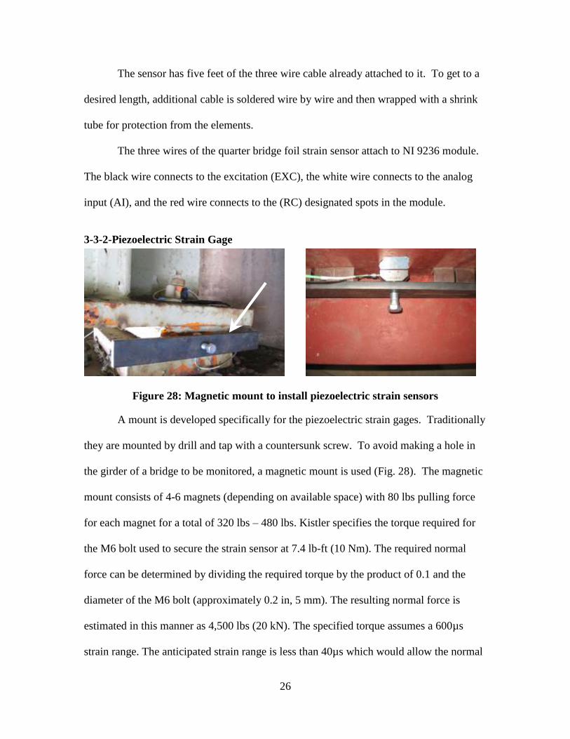
3-3-2-Piezoelectric Strain Gage
Figure 28: Magnetic mount to install piezoelectric strain sensors
A mount is developed specifically for the piezoelectric strain gages. Traditionally
they are mounted by drill and tap with a countersunk screw. To avoid making a hole in
the girder of a bridge to be monitored, a magnetic mount is used (Fig. 28). The magnetic
mount consists of 4-6 magnets (depending on available space) with 80 lbs pulling force
for each magnet for a total of 320 lbs – 480 lbs. Kistler specifies the torque required for
the M6 bolt used to secure the strain sensor at 7.4 lb-ft (10 Nm). The required normal
force can be determined by dividing the required torque by the product of 0.1 and the
diameter of the M6 bolt (approximately 0.2 in, 5 mm). The resulting normal force is
estimated in this manner as 4,500 lbs (20 kN). The specified torque assumes a 600µs
strain range. The anticipated strain range is less than 40µs which would allow the normal

27
force to be scaled accordingly to 300 lbs. This is achieved by only four magnets. A 1 inch
by 12 inch by 0.25 inch steel bar is bridged over the magnets. A screw threaded through
the steel bar is used to apply the normal force onto the sensor.
There is a one foot length green cable attached to the sensor, and attached on the
other end to the model 571A5 range capacitor and model 558 impedance converter. A
general purpose cable with BNC connector is then connected between the impedance
converter and the NI 9234 module.
3-3-3-Piezoelectric Accelerometer
Junction boxes in the conduit are mounted to the bottom of the concrete bridge
deck using a hammer drill and screws ensuring that the junction box is firmly fixed to the
underside of the deck. The accelerometers are mounted inside the junction boxes with
threaded studs screwed into holes drilled and tapped into the junction box itself.
From the sensor, there is a 2-pin top connection that connects to a one foot length
2-socket boot connector to BNC jack cable. This one foot cable then connects to a BNC
to BNC cable ordered to desired length. The BNC end simply screws into the AI terminal
of the NI 9234 module.
3-3-4-Capacitance Accelerometer
The capacitance accelerometers are also located in the junction boxes under the
bridge deck. These sensors are attached to a plastic piece that is drilled and taped to
accept the capacitance accelerometer. The plastic piece is glued to the inside of the
junction box.

28
Figure 29: A power supply to power the capacitance accelerometers (picture from
vendor)
The output cables are attached to the sensor by twist connection. A power supply
type B24G30 produced by Acopian Company was used to provide the required power for
capacitance accelerometers (Fig. 29). The power supply B24G30 contains five external
screw/ports including +out, -out, LAC, NAC, and ground. Three ports including LAC,
NAC, and ground are used to connect the power supply to the power cord. The
capacitance accelerometer cable has four wires including power (red wire), acceleration
signal (white wire), temperature signal (yellow wire), and ground (black wire).The power
wire of capacitance accelerometer is connected to the +out of power supply via the red
lead wire. The signal wires of capacitance accelerometer are connected to the channels of
NI 9206 via the white and yellow wires. White and yellow wires are collecting
acceleration and temperature signals, respectively, in the capacitance accelerometer. The
common ground of NI 9206 module (COM) and ground wire of capacitance
accelerometer (black wire) both are connected to the –out of power supply.

29
3-3-5-Resistance Temperature Detector
Figure 30: An installed resistance temperature detector on the Meriden Bridge
Locations on the girder for temperature sensors must be prepped and cleaned
similarly to the locations of strain sensors. Then the temperature sensors are mounted to
the girder using the epoxy. Figure 30 shows one of the installed temperature sensors on
the Meriden Bridge.
The RTD sensors have integrated cables. The cable length can be specified and
ordered to desired length. The output end of the cable has four wires, two are red and
two are white wires. These connect to the NI 9217 module. The red wires are attached to
the terminals for excitation (EX) and RTD+. The white wires are attached to the spots
for RTD- and common (COM).
4-BWIM
4-1-BWIM methodology
The BWIM methodology uses strain measurements from the steel girder of the
slab-on-girder highway bridge to determine gross vehicle weight, speed, axle spacing and
axle weights. The method does not require development of a bridge model or influence
line. The unique aspect of the proposed BWIM method in this study is the non-intrusive

30
(i.e. no sensors in the pavement) calculation of truck characteristics for a single-span
highway bridge, using only strain measurements of the steel girders beneath the bridge.
The proposed method builds on the theory for determining gross-vehicle weight from the
work of Ojio and Yamada (Ojio and Yamada, 2002) and the findings of Cardini and
DeWolf (2009). It is further documented in Wall et al. (2009).
The BWIM method employed here assumes that the single-span bridge behaves
as a simply supported beam neglecting the spatial behavior of the multi-lane bridge;
assumes the truck loads are applied to the bridge by the truck axles and can be modeled
as a group of point loads moving across the simply supported beam at fixed spacing and
constant speed; and neglects both bridge and truck dynamics.
The unique aspect of this method is the use of the second time derivative of the
measured strain to identify, with large negative spikes or peaks, when the truck axles pass
over the center of bridge. Truck speed is determined from the time, 1t , it takes the first-
axle of the truck to travel from the start of the bridge to the mid-span of the bridge such
that
)(2 1t
Lv (1)
Where v is the speed of the truck (ft/sec), L is the length of the bridge (ft) and 1t is
the time it takes for the first axle of the truck to travel from the start of the bridge to the
mid-span (sec). The sensors can be located at any location along the length of the bridge
and, as observed from the theory of influence lines, will read peak strain values when the
point load crosses the center of the bridge. It is optimal to place the strain sensors at the
center of the bridge as this provides the largest amplitude of strain response.

31
The second derivative of the strain also provides the times when each of the remaining
axles pass over the mid-span of the bridge; t2, t3, t4 and t5 for a 5-axle truck. The product
of time difference between these times and the calculated speed provides the truck’s axle
spacing, xn, as given by
)( 1 nnn ttvx , n= 1,2,…,N-1 (2)
where xn is the distance between the n-1 and nth
axles, and tn is the time it takes for
the nth
axle to reach the mid-span of the bridge after the truck first enters the bridge, and
N is the total number of axles of the truck.
Gross vehicle weight is then determined from the method of Ojio and Yamada,
(2002) as described subsequently. The response wave is the strain response of the bridge
to a truck traveling over the bridge. The response wave can be defined mathematically as
the strain at a specific location of the bridge due to multiple point loads traveling over the
bridge. The response wave is written as
N
n
nn xxfPx1
)( (3)
Where Pn is the weight, or magnitude, of the nth
axle, assumed to be a point load,
xn is the distance between axles, and )( nxxf is the influence line of the simply
supported beam. The influence area, A, of a single truck passing over the bridge is
defined as
dxxxA
(4)
Substituting Eq. 3 into Eq. 4 and rearranging slightly gives
N
n
nn dxxxfPA1
)( (5)

32
Recognizing that the Gross Vehicle Weight (GVW) can be written as
N
n
nPGVW1
(6)
allows Eq. (5) to be simplified as
N
n
n dxxxfGVWA1
)( (7)
For trucks with the same axle configuration the term in the summation is a constant, such
that
N
n
n dxxxf1
)( (8)
This constant α can be substituted into Eq. (7) and written as
GVW
A (9)
This method requires the GVW of a test truck to be known and then the GVW of any
unknown weight truck can be determined knowing that
u
u
k
k
GVW
A
GVW
A (10)
where Ak and GVWk are the calculated area and reference gross vehicle weight for a test
truck of known weight, and Au and GVWu are the calculated area and gross vehicle weight
for a truck with unknown weight. Equation (10) can be arranged so that
k
k
u
u GVWA
AGVW (11)
The ratio of GVWk to Ak is defined as the calibration constant β where
k
k
A
GVW (12)

33
Thus, the GVW of the unknown truck is then determined as
uu AGVW (13)
Where A can be written in terms of ε(t), again where vtx , and written in discrete form
such that
M
i
tiM
tvdttvtA
1
)( (14)
where Δt is the discrete sample time of the strain measurement, and M is the total number
of measurements needed for the truck to cross the bridge. The axle weights are relative to
the magnitudes of the peaks of the second time derivative of the strain as each axle passes
over the center of the bridge span. In practice BWIM is often conducted over a short
period of time where temperature variation can be neglected. For a system that will be in-
place through seasonal variations the effect of the temperature should be examined. In
this study, temperature measurements at multiple locations will be used to assess the
effect of temperature variations and thermal gradient on the accuracy of the BWIM data.
4-2-Field study
A pilot study, conducted on December 13, 2011, included an initial field test
using a loaded 5-axle truck of known weight making multiple passes over the prototype
bridge system. The purpose of this initial field test was for initial calibration of the
BWIM method. A secondary purpose of the pilot study was to gather information on the
various sensor responses, assess the ability to calculate speed data and evaluate the
variability in the results from applying the calibration to the initial test vehicle
calculations.

34
4-2-1-Truck of known weight
The test vehicle was a five-axle semi-trailer with air-ride suspension (Fig. 31).
The vehicle was loaded, and then was measured to weigh 68,600-lbs (31116-kg). The
static weight was obtained at the weigh station on I-91 northbound in Middletown prior
to testing, operated by the State Police. A total of twelve passes were made by the truck
during the field test: five passes in the middle lane and seven passes in the slow lane.
The truck driver attempted to vary the speed at 50-mph (80-kph), 55-mph (88-kph), and
60-mph (96-kph) according to instructions and based on traffic.
Figure 31: Truck of known weight
4-3-Test results and evaluation
The speed of the truck was recorded both from reading a commercial navigation
system installed in the truck and derived from a portable GPS unit incorporating radar,
receiver and aerial map installed in the truck for the purpose of this study. The speeds
collected from both GPS based devices were well correlated with a maximum difference
of 1 mph. Therefore the speed recorded from the commercial navigation system was
used as the “ground-truth” or “actual” truck speed for comparison with the speed
calculated from the bridge response. The speed of the truck was calculated based on
bridge strain data and using Equation (1). A comparison between the measured (GPS)

35
and calculated (bridge) speeds is presented in Table 1. The average difference between
measured and calculated speed was 4.5% and indicates that the calculated speed was in
reasonable agreement with that recorded by the “actual” speed data.
Table 1- Comparison of Measured and Calculated Truck Speed
Run Lane
Attempted
Speed* Measured
Speed
(mph)
Calculated
Speed
(mph)
Difference%
(mph)
1 Middle 60 58 62 6.5
2 Middle 60 62 66 6.6
3 Middle 60 62 65 4.8
4 Middle 60 63 65 3.1
5 Middle 60 63 66 4.2
6 Slow 60 62 65 5.3
7 Slow 60 61 62 2.3
8 Slow 60 62 64 2.9
9 Slow 60 62 57 7.5
10 Slow 60 63 65 3.5
11 Slow 55 55 57 4.1
12 Slow 50 49 51 3.9
* the attempted speed is the speed the driver was instructed to drive.
The performance of the two accelerometer technologies, piezoelectric and
capacitive, is examined in the time domain and frequency domain as shown in Figs. 32(a)
and (b). The data shown are from accelerometers placed on girder 6 at mid-span with the
truck traveling in the slow lane at a speed of 62-mph (100-kph). An eight-pole low-pass
filter with a 100 Hz cutoff frequency was used to reduce the effect of noise on the
acceleration data. The piezoelectric and capacitive accelerometers have a frequency
range of 0.1 to 200 Hz and 0 to 250 Hz, respectively. From the time domain plots the
two accelerometers are observed to have similar noise levels and provide comparable
measurements. A time lag of 0.019 seconds was observed in the capacitive
accelerometers relative to the piezoelectric accelerometers (inset in Figure 32(a)). In the

36
frequency domain the two sensor technologies provide similar performance above 3 Hz,
while the piezoelectric accelerometer rolls off at lower frequencies. Neither
accelerometer can capture the crossing of truck axles over the midspan. It is expected that
accelerometers with larger bandwidth will be able to measure this large negative
acceleration when the axles pass over the center of the bridge and can be used as
redundant or replacement measurements for the truck speed. Piezoelectric accelerometers
with higher frequency range were installed to examine the benefit of larger bandwidth for
the acceleration measurements.
(a)
10-1
100
101
102
-180
-170
-160
-150
-140
-130
-120
-110
-100
Frequency(1/sec)
Am
plit
ude(D
essib
le)
Piezo-Accelerometer
Capacitive Accelerometer
(b)
Figure 32: Piezoelectric accelerometer vs. capacitive accelerometer data: (a) time
history for truck crossing; (b) auto power spectral density of acceleration.
The performance of the two types of strain gage technologies, foil strain gage and
piezoelectric strain gage, are compared in Figs. 33(a) and (b) in the time domain and
frequency domain, respectively. These data are measured from the gages on girder 6 at
the North bearing. A comparison in time domain shows the time decay observed in the
piezoelectric strain gauge signals resulting from the signal conditioner used for this
sensor. The attenuation at low frequencies was observed in the frequency domain as

37
well. The data from both sensor technologies are in good agreement from 0.5-10 Hz. A
large peak in the autopower spectral density functions of both strain sensors was
observed at 60 Hz corresponding to ground loop noise. An eight-pole low-pass filter
with a 30 Hz cutoff frequency was applied to reduce the effect of the ground loop noise at
60 Hz. The strain measurements from the foil-type strain sensors are used for the BWIM
measurements in this report.
44 44.5 45 45.5 46 46.5 47 47.5 48-2
-1.5
-1
-0.5
0
0.5
1
1.5
2
Time (Second)
Str
ain
(mic
rostr
ain
)
Piezo-Strain gage
Foil-Strain gage
(a)
10-1
100
101
102
-100
-90
-80
-70
-60
-50
-40
-30
-20
-10
Frequency(1/sec)
Am
plit
ude(D
essib
le)
Piezo-Strain gage
Foil-Strain gage
(b)
Figure 33: Piezoelectric strain sensors vs. foil Strain gages data: (a) time history for
truck crossing; (b) autopower spectral density of acceleration.
The axle spacing of the test truck is calculated using the calculated speed and
Equation (2) with time intervals based on the large negative spikes in the second
derivative of the strain history, as shown in Fig. 34. Table 2 presents the measured and
calculated axle spacing for the middle lane and slow lane. The prediction of axle spacing
for Run 6 is incomplete for the last three axles due to the presence of multiple vehicles on
the bridge. The axle spacing is slightly overestimated in comparison to actual
measurements, due to an overestimation bias in the speed calculation, as observed in
Table 1. This overestimation demonstrates both the sensitivity and importance of the
speed calculation.

38
44.4 44.6 44.8 45 45.2 45.4
-1000
-800
-600
-400
-200
0
200
400
600
Time (Second)
d2(s
train
)/dt2
Figure 34: Negative spikes in second derivative of strain measurement when the
truck axles pass over the mid-span of the bridge
For calibration, the ratio of GVWk to Ak, called β, is calculated from Equation (12)
for each pass in the middle lane and each pass in the slow lane, based on the static weight
of the truck (68,600-lb) and the measured strain at the midspan of girders 6 and 4,
respectively. The calibration constant β calculated (as the average of these values), is
0.032-lb/ft for the middle lane, and 0.034-lb/ft for the slow lane. The standard deviation
of β is 0.0036-lb/ft, which demonstrates the repeatability of the method.
Table 2- Comparison of measured and calculated truck axle spacing
Axles Meas.
Ft
(meter)
Calculated (Middle Lanes) ft
(meter)
Calculated (Slow Lanes)
Ft (meter)
1 2 3 4 5 6 7 8 9 10 11 12
1 to 2 17 (5.1)
17.6
(5.4)
17.9
(5.4)
17.7
(5.4)
17.6
(5.4)
17.7
(5.4)
17.1
(5.2)
17.4
(5.3)
17.3
(5.3)
17.3
(5.3)
17.4
(5.3)
17.4
(5.3)
17.5
(5.3)
2 to 3 4.2
(1.3)
5.3
(1.6)
5.4
(1.6)
5.3
(1.6)
5.7
(1.7)
6
(1.8) *
5.5
(1.7)
5.7
(1.7)
5.6
(1.7)
5.4
(1.6)
5.5
(1.7)
5.4
(1.6)
3 to 4 30.6
(9.3)
31.7
(9.6)
31
(9.4)
31
(9.4)
30.6
(9.3)
31.7
(9.6) *
31
(9.4)
30.5
(9.3)
34.4
(10.5)
31.1
(9.5)
31.1
(9.5)
30.6
(9.3)
4 to 5 4.1
(1.2)
5.5
(1.7)
5.5
(1.7)
5.3
(1.6)
5.4
(1.6)
5.4
(1.6) *
5.3
(1.6)
5.5
(1.7)
5.4
(1.6)
12.4
(3.7)
5.5
(1.7)
5.2
(1.6)
1st Axle 2nd & 3rd Axles
4th & 5th Axles

39
“*” issues due to presence of multiple trucks on the bridge
Based on the selection of β, the weight of the truck of known-weight for different
runs is calculated using Equation (13). These results are presented in Table 3. The
measured and calculated weight of the truck are in a well agreement in most of the cases
and the average difference between the calculated and measured weight was respectively,
8.0% and 7.8 % for the middle and slow lanes. While these weights were calculated
using the constant β, calculated from the same data set, the weight data are useful to
ascertain the variation when applied to the variation from the test truck. Applying this
technique, the outcome was a comparable β. Additional test runs are planned to apply the
calibration factor, β, to different vehicles and a larger number of vehicles.
Table 3- Comparison of measured (68,600-lb (3116-kg)) to calculated truck weight
Middle Lane Slow Lane
Runs 1 2 3 4 5 6 7 8 9 10 11 12
Weight lb
(kg)
66551
(3018
7)
68780
(3119
8)
62120
(2817
7)
65157
(2955
4)
84206
(3819
5)
70008
(3175
5)
59488
(2698
3)
70538
(3199
5)
64001
(2903
0)
66805
(3030
2)
85386
(3873
0)
70488
(3197
2)
Difference% 2.99 0.26 9.45 5.02 22.75 2.05 13.28 2.83 6.7 2.62 24.47 2.75
5-BHM
5-1-BHM methodology
To account for the variability associated in calculating the desired damage
measure, a probabilistic BHM approach can be adopted to detect global damage in the
highway bridge. This section defines damage measures used to identify structural
changes in the bridge structure, describes the probabilistic framework used to assess any
changes in the bridge condition, and presents a means to incorporate temperature and
truck weight data in the probabilistic framework to enhance the accuracy of the BHM.

40
In order to assess the structural integrity of the bridge, damage measures (DMs)
corresponding to the structural health of the bridge are determined from the structure’s
dynamic response to truck traffic. The basis for this method is that a healthy DM (DMH)
can first be determined as a baseline. At subsequent times, the current DM (DMC) can be
determined and compared to the healthy case. For this bridge the DMs, similar to those
used in Cardini and DeWolf (2009), are the peak strain, strain distribution over the eight
steel girders, calculated location of neutral axis, and estimated fundamental natural
frequency of the bridge which is calculated as the first peak of the power spectral density
function (PSD).
The first damage measure is the peak strain measured at the bottom of the eight
steel girders each time a truck crosses. The peak strain damage measure is determined as
the strain in each of the eight girders at the time, tpk, of the maximum peak strain over all
of the girders. The first damage measure can be determined as
pkii tDM 1 (15)
where 1
iDM is the peak strain on all eight girders i=1,2,…,8 at the time tpk, i is
the strain reading of the bottom strain sensor at the midspan of each girder. If the peak
strain increases, this can be an indication of local damage (e.g. fatigue cracking) or
damage in an adjacent girder; whereas, if the peak strain decreases, this can indicate
damage somewhere on the length of that girder.
The second damage measure is the distribution of the strain in the eight girders as
a truck passes over the bridge. This DM is an indicator of how the load is distributed to
each of the girders of the indeterminate structural system. The strain distribution is
determined as

41
8
1
2
i
pki
pki
i
t
tDM
(16)
Where 2
iDM is the distribution factor for the ith
girder. If the strain distribution
changes, this is an indication that the load path of the indeterminate structural system of
the bridge has changed and members under less strain may be damaged, while members
under larger strain are likely undamaged (or less damaged).
The third damage measure is the location of the neutral axis at each girder. If the neutral
axis rises into the slab there can be tension and cracking of the concrete bridge deck. If
the neutral axis lowers there could have already been failure of the deck.
ii
iiiii
dddDM
ˆ
ˆ3 (17)
where 3
iDM is the distance from the bottom of the girder to the neutral axis, di is
the distance from the bottom of the girder to the bottom sensor, id is the distance from
the bottom of the girder to the top sensor, and i is the strain reading at top sensor of each
girder.
The final damage measure considered in this study will be the measured bridge natural
frequencies.
jj fDM 4 (18)
where the natural frequencies fj are determined from the peaks of the auto-power
spectral density functions of the measured acceleration responses as given by (Bendat and
Piersol, 2000)
2
,1
lim2 TfXET
fG kT
xx (19)

42
where Gxx is the auto-power spectral density function of x(t), T is the record length
taken to be a sufficiently long record, E is the expected value operator, and kX is the
finite Fourier transform of the measured acceleration tx for the kth
ensemble. The
bridge natural frequencies are directly related to the mass and stiffness of the bridge
structure. Therefore, a change in the natural frequency is an indicator that the stiffness
(or mass) of the structural system has changed.
5-2- Probabilistic approach
The DMs, calculated from measured bridge responses from traffic loading, are
neither deterministic nor constant and can be considered to be random variables with a
Gaussian distribution. As such, not just one realization of each DM is calculated, but a
set of n DMs are determined. The mean and variance of the original set of data for the
healthy structure is determined so that the probability density function of DMH is known.
At each current period of time, n new DMs are calculated and the mean and variance are
determined as before so that the probability density function of DMC is now known. The
basis for this probabilistic method is then to compare the distribution of a current DM to
the baseline DM to determine if there is a change in the underlying distribution, thus
indicating a potential change in the structure and possible damage (23).
The Student’s t-test is used to compare the two distributions of each of the DMs. It is
assumed that the variance of the two samples is unequal and an adaptation of the
Student’s t-test called Welch’s t-test is used. Welch’s t-test defines the statistic t as
CH XX
CH
s
XXt
(20)
where

43
C
C
H
H
XX n
s
n
ss
CH
22
(21)
HX and CX , 2
Hs and 2
Cs , and Hn and Cn are the mean, variance, and sample
size, respectively, of the healthy and current distributions.
The t-distribution can be used to test the null hypothesis that the two DM means are equal
at a certain significance level. If the current t-statistic is less than the critical t value for a
particular level of significance, the null hypothesis is rejected; this indicates a statistically
significant change in the mean and potential for damage in the structure. If the current t-
statistic is greater than the critical t value for a particular level of significance, the null
hypothesis cannot be rejected; this indicates no statistically significant change in the
mean and that the structural integrity of the current scenario should be assumed the same
as the structural integrity of the baseline scenario.
To provide further insight into the statistical test, the p-values instead of a general
‘pass’ or ‘fail’ result are observed. The p-value is the probability of observing an event at
least as extreme as the one actually observed, given that the null hypothesis is true. The
p-value for a two-tailed Welch’s t-test can be calculated as:
)](1[2 tp (22)
where Φ is the standard normal operator. Generally one rejects the null
hypothesis when the p-value is smaller than or equal to the significance level.
5-3-Accounting for thermal and truck weight effects in BHM
While the probabilistic approach can accommodate inherent variability in the
system, the ability to identify structural damage can be enhanced by accounting for the
variability in DMs due to measurable parameters that result in variability of the response

44
and DM. In particular, temperature measurements have been used in previous research to
account for variability due to environmental conditions (Olund, 2004). Thermal changes
in bridge structures have been observed to cause changes in the structure’s boundary
conditions which can lead to changes in the DMs. This study will further explore the
variability and correlation of DMs with characteristics of the truck traffic actually passing
over the bridge. For example, the weight of the truck or length of the truck may have an
influence on the DMs that can be characterized.
One possible approach to account for thermal and truck weight effects on the
damage measures that has been applied successfully to other bridges in Connecticut for
BHM is the use of conditional distributions of the DMs. The temperature range can be
divided into bins where measured events are separated. Further, each temperature bin
can also be subdivided into truck weight bins, for example. When a probabilistic BHM
method is applied, the distribution of the DM from each temperature and truck weight bin
of the baseline time period is compared to that of the same temperature and truck weight
bin for the current time period to see if that distribution has varied. A temperature and
truck weight dependent p-value,2121 WWWTTTp can then be determined. The associated
temperature and truck weight dependent p-values can be equally weighted and averaged
over all of the temperature bins such that
N
n
M
m
mWWmWnTTnTpMN
p1 1
)1()1(
11 (23)
where p is the average p-value for all temperatures and truck weights, N is the
number of temperature bins, M the number of truck weight bins, ΔT is the size of the
temperature bin and ΔW is the size of the truck weight bin. The p value is then compared

45
to a prescribed significance level to determine if the null hypothesis, that the means of the
various distributions are equal, can be rejected.
6-CONCLUSION
The prototype BHM/BWIM system including sensors, data acquisition system
deployed on the Meriden Bridge, BWIM/BHM methodology, and results of BWIM test
were described.
A new BWIM method that provides for non-intrusive means of obtaining weigh-
in-motion data is presented and an initial field test was conducted as part of a pilot study
where a truck of known-weight conducted multiple passes over the instrumented bridge.
Based on this initial field test, the system was calibrated and weigh-in-motion data (i.e.
speed, axle-spacing and weight data) were calculated. Foil-type strain sensors are
observed to provide better strain measurements during truck crossings than the
piezoelectric strain sensors due to a larger time constant. Both accelerometers provide
similar measurements above 3 Hz. The calculated speed, axle spacing and weight data are
in reasonable agreement with the measured data. Inaccuracies due to multiple vehicle
presence on the bridge can be addressed by considering the response of multiple girders.
Truck speed measurements, observed to be critical in the accurate calculation of axle
spacing and weight, can be enhanced by using accelerometers with larger bandwidth. The
second phase of the project will explore these enhancements and validate the BWIM
methodology with vehicles from the traffic stream and variations in temperature.
Additionally, BWIM data collected continuously will be validated periodically
throughout the project to ensure the system is robust and stable in operation. To evaluate
the BHM capabilities of the system, the bridge health monitoring data will be assimilated

46
into the network of long-term bridge monitoring in Connecticut where the damage
measures will be determined and saved to a CTDOT repository for analysis over time.
The proposed BHM method to be used in the dual BHM/BWIM system is
described. The components of the BHM method, including DMs, a probabilistic
framework, and the mechanism to leverage BWIM data to improve accuracy of BHM,
are presented.
REFERENCES
ASTM E1318 Road and Paving Standards, (2009) “Standard Specification for Highway
Weigh-In-Motion (WIM) Systems with User Requirements and Test Methods,”
Designation: E 1318-09.
Bendat, J.S, Piersol, A.G. Random Data: Analysis and Measurement Procedures. John
Wiley and Sons, Inc., New York, 2000.
Cardini, A.J. and DeWolf, J.T. (2009). “Long-Term Structural Health Monitoring of a
Multi-girder Steel Composite Bridge Using Strain Data,” submitted for publication.
Cardini, A.J. and DeWolf, J.T. (2009). “Development of a Long-Term Bridge Weigh-In-
Motion System for a Steel Girder Bridge in the Interstate Highway System,” submitted
for publication.
Caicedo, J., Dyke, S.J. and Johnson, E.A. (2000). “Health Monitoring Based on
Component Transfer Functions,” Advances in Structural Dynamics, (Ko, J.M. and Y.L.
Xu, eds.) Vol. II, pp. 997-1004.
Chang, F.K. (2000). Structural Health Monitoring 2000. Technomic, Lancaster, PA.

47
Chakraborty, A. and Okaya, D. (1995). “Frequency-Time Decomposition of Seismic
Data using Wavelet-Based Methods,” Geophysics, Vol. 60, No. 6, pp. 1906-1916.
Christenson, R, Bakulski, S., and McDonnell, A. (2011), “Establishment of a Dual-
Purpose Bridge Health Monitoring and Weigh-in-Motion System for a Steel Girder
Bridge”, Transportation Research Board 90th
Annual Meeting, Washington, DC
ASTM E1318 Road and Paving Standards, (2009), “Standard Specification for Highway
Weigh-In-Motion (WIM) Systems with User Requirements and Test Methods”, E 1318-
09.
Connecticut Academy of Science and Engineering (2008). “A Study of Weigh Station
Technologies and Practices,” a report by the Connecticut Academy of Science and
Engineering for the Connecticut Department of Transportation, November 2008.
DeWolf, J.T., Cardin, A.J., Olund, J.K. and D’Attilio, P.F. (2009). “Structural Health
Monitoring of Three Bridges in Connecticut,” Transportation Research Board 88th
Annual Meeting, Washington DC, January 11-15, 2009.
Doebling, S.W., Farrar, C. R., Prime, M. B. and Shevitz, D. W. (1996). “Damage
Identification and Health Monitoring of Structural and Mechanical Systems from
Changes in their Vibration Characteristics: A Literature Review,” Report LA: I3070-MS,
Los Alamos National Laboratory, NM.
Farrar, C.R., Duffy, T.A., Doebling, S.W. and Nix, D.A.. “Vibration-Based Structural
Damage Identification,” In Proceedings of the 2nd International Workshop on Structural
Health Monitoring, 2nd International Workshop on Structural Health Monitoring,
Stanford, CA, 1999, pp. 764-773.
Farrar, C. R., Baker, W. B., Bell, T. M., Cone, K. M., Dading, T. W., Duffey, T. A.,
Ekiund, A. and Migliori, A. (1994). “Dynamic Characterization and Damage Detection
in the I-40 Bridge over the Rio Grande,” Las Alamos Report LA- 12767-MS UC-906,
June 1994, 15, pp. 3.
Farrar, C. R. and Doebling, S. W. (1997). “Lessons Learned from Applications of
Vibration Based Damage Identification Methods to Large Bridge Structure,” Structural
Health Monitoring: Current Status and Perspectives, 351-370, ed. F. K. Chang,
Technomic Pub. Lancaster, PA.
FHWA (Federal Highway Administration) 2001. “Traffic Monitoring Guide,” Office of
Highway Policy Information, May 1, 2001.
FHWA (Federal Highway Administration) 2005. “Safe, Accountable, Flexible, Efficient
Transportation Equity Act: A Legacy for Users, A Summary of Highway Provisions.”
Jacob, B. (2002). “Weigh-in-Motion of Axles and Vehicles for Europe,” Final Report of
the Project WAVE, LCPC, Paris, France.

48
Moses, F. (1979). “Weigh-in-Motion System using Instrumented Bridges,” American
Society of Civil Engineers, Transportation Engineering Journal, v 105, n 3, May, 1979,
pp. 233-249
McDonnell, A.M. (2000). “Evaluation of Quartz-Piezoelectric WIM Sensors: Second
Year Study,” NATMEC 2000, August 29, 2000, Madison, WI, 13 pages.
Olund, J.K., Cardini, A.J., D’Attilio, P., Feldblum, E. and DeWolf, J.T. (2006).
“Connecticut’s Bridge Monitoring Systems,” NDE Conference on Civil Engineering, St.
Louis, MO, 173-179.
Ojio, T. and Yamada, K. “Bridge Weigh-In-Motion Systems Using Stringers of Plate
Girder Bridges,” Pre-Proceedings of the Third International Conference on Weigh-In-
Motion, (2002): 209-218.
Olund, J. Long Term Structural Health Monitoring of Connecticut’s Bridge
Infrastructure with a Focus on a Composite Steel Tub-Girder Bridge. M.S. Thesis. The
University of Connecticut, 2006.
Scianna, A. and Christenson, R. “Implementation of a Probabilistic Bridge Health
Monitoring Network on a Highway Bridge,” Fifth New York City Bridge Conference,
August 17-18, 2009.
Salawu, O.S. and Williams, C. (1995). “Review of Full-Scale Dynamic Testing of
Bridge Structures,” Eng. Struc. 17(2): 113-121.
Salawu, O.S. (1997). “Detection of Structural Damage through Changes in Frequency
Review,” Eng. Struct. 19(9)718-723.
Transportation Research Board, Research in Progress, “Bridge Weigh-in-Motion (B-
WIM) System Testing and Evaluation”, website
http://rip.trb.org/browse/dproject.asp?n=13137, accessed July 23, 2010.
Wall C. and Christenson, R. (2009). “A Bridge Weigh-In-Motion Case Study in
Connecticut,” to be submitted to the Annual Meeting of Transportation Research Board,
Washington D.C.
Connecticut Permanent Long-Term Bridge Monitoring Network, Volume 1: Monitoring
of Post-Tensioned Segmental Concrete Box-Girder Bridge - I-95 over the Connecticut
River in Old Saybrook (Bridge # 6200). (pdf 1179 kb), Final Report, Adam Scianna,
Stephen Prusaczyk, Zhaoshuo Jiang, Richard E. Christenson, John T. DeWolf, CTDOT
Report No. CT-2256-2-13-2,August 2014
Connecticut Permanent Long-Term Bridge Monitoring Network Volume 2: Monitoring
of Curved Post-Tensioned Concrete Box-Girder Bridge -I-384 WB Over I-84 in East

49
Hartford (Bridge # 5686) (pdf 785 kb), Final Report, Adam Scianna, Stephen Prusaczyk,
Zhaoshuo Jiang, Richard E. Christenson, John T. DeWolf, Jeong-Ho Kim CTDOT
Report No. CT-2256-3-13-4,August 2014
Connecticut Permanent Long-Term Bridge Monitoring Network Volume 3: Monitoring
of a Multi-Steel Girder Composite Bridge - I-91 SB over the Mattabesset River in
Cromwell (Bridge # 3078) (pdf 836 kb), Final Report, Shelly Plude, Stephen
Prusaczyk,Adam Scianna, Zhaoshuo Jiang, Richard E. Christenson,Jeong-Ho Kim, John
T. DeWolf CTDOT Report No. CT-2256-4-13-5,August 2014
Connecticut Permanent Long-Term Bridge Monitoring Network Volume 4: Monitoring
of Curved Steel Box-Girder Composite Bridge- I-84 EB Flyover to I-91 NB in Hartford
(Bridge # 5868) (pdf 1031 kb), Final Report, Adam Scianna, Stephen Prusaczyk,
Zhaoshuo Jiang, Richard E. Christenson, John T. DeWolf, CTDOT Report No. CT-2256-
5-13-6,August 2014
Connecticut Permanent Long-Term Bridge Monitoring Network Volume 5: Wireless
Monitoring of the Hung Span in a Large Truss Bridge -I-95 NB over the Thames River
in New London (Bridge # 3819) (pdf 912 kb), Final Report, Adam Scianna, Stephen
Prusaczyk, Richard E. Christenson, John T. DeWolf, CTDOT Report No. CT-2256-6-13-
7,August 2014
Connecticut Permanent Long-Term Bridge Monitoring Network Volume 6 : Monitoring
of a Continuous Plate Girder Bridge with Load Restrictions - Route 15 Over the
Housatonic River in Stratford (Bridge # 761) (pdf 223 kb), Final Report, Stephen
Prusaczyk, Harinee Trivedi, Richard E. Christenson, John T. DeWolf, CTDOT Report
No. CT-2256-7-13-8,August 2014
Connecticut Permanent Long-Term Bridge Monitoring Network Volume 7: Lessons
Learned for Specifications to Guide Design of Structural Health Monitoring Systems
(pdf 3005 kb), Final Report, Richard E. Christenson, John T. DeWolf, Stephen
Prusaczyk, CTDOT Report No. CT-2256-8-13-9,August 2014