Information in the Term Structure: A Forecasting

Perspective�

Hitesh Doshi Kris Jacobs Rui Liu

University of Houston

November 18, 2016

Abstract

Cochrane and Piazzesi (2005) and Du¤ee (2011a) �nd that information not captured by

traditional term structure factors helps predict excess bond returns. We show that when

estimating no-arbitrage a¢ ne term structure models, aligning in-sample and out-of-sample

objective functions results in term structure factors that capture similar information that

remains hidden from existing approaches. Speci�cally, the estimates of the third term

structure factor radically di¤er. Consistent with Cochrane and Piazzesi (2005), this factor

con�rms the importance of the fourth principal component of yields for forecasting the term

structure. The new objective function leads to substantial improvements in forecasting

performance. Model term premiums are higher and expected future short rates are lower.

JEL Classi�cation: G12, E43

Keywords: term structure; forecasting; loss function; state variables; hidden factor.

�We would like to thank Anh Le, Drew Creal, Raymond Kan, Zhan Shi, Bin Wei, Jean-Sébastien Fontaine,participants at the San Francisco Fed-Bank of Canada Conference on Fixed Income Markets, and especially FrankDiebold for useful comments. This paper was previously circulated under the title "Loss Functions for ForecastingTreasury Yields". Correspondence to: Kris Jacobs, C.T. Bauer College of Business, University of Houston, 334Melcher Hall, Tel: (713) 743-2826; Fax: (713) 743-4622; E-mail: kjacobs@bauer.uh.edu.

1

1 Introduction

Modeling the term structure is a topic of great practical importance for investors as well as

monetary policy makers. The term structure contains valuable information about expectations

of future interest rates and term premia, and the identi�cation of these components critically

rests on the speci�cation of the term structure model. Much of the term structure literature

therefore focuses on model speci�cation and estimation.

We depart from the existing literature by documenting the importance of the information

used in the estimation of the term structure model. Speci�cally, while the cross-sectional and

time-series dimension of our sample is very similar to the existing literature, we di¤er by con-

sidering a di¤erent objective (loss) function, which is explicitly motivated from a forecasting

perspective. This approach is motivated by the literature on bond return prediction. Cochrane

and Piazzesi (2005) and Du¤ee (2011a), among others, argue that a hidden factor not captured

by the traditional level, slope, and curvature factors helps in predicting excess bond returns.

We build on this insight and estimate no-arbitrage term structure models by specifying a loss

function at the estimation stage which is motivated from a forecasting perspective and aligned

with the out-of-sample evaluation measure. Our null hypothesis is that when we estimate the

no-arbitrage model using this alternative loss function, the model properties will capture and

re�ect this hidden information.

It is well known in the statistics literature that the speci�cation of the loss function critically

in�uences model estimates and properties. Indeed, the speci�cation of a loss function implicitly

amounts to the speci�cation of a statistical model, because the loss function determines how

di¤erent forecast errors are weighted (see Engle, 1993; Granger, 1993; Weiss, 1996; Elliott and

Timmermann, 2008). Since the loss function is an important element in the process of delivering

a forecast, it is an integral part of model speci�cation. If a particular criterion is used to evaluate

forecasts, it should also be used at the estimation stage.1 Estimating a model under one loss

1An extensive literature studies the theoretical properties of optimal forecasts under asymmetric loss functions

2

function and evaluating it under another amounts to changing the model speci�cation without

allowing the parameter estimates to adjust.

Motivated by these insights, we estimate A¢ ne Term Structure Models (ATSMs) while align-

ing the loss functions for in-sample estimation and out-of-sample evaluation.2 We estimate the

model by minimizing the squared forecasting errors for a given forecast horizon, and we refer to

these estimates as based on the forecasting loss function. We compare the implications of these

estimates with the implications of estimates obtained by minimizing the mean-squared error loss

function based on current yields, which we refer to as the standard loss function. We analyze how

the choice of loss function a¤ects model implications for factor dynamics, expected short rates

and term premia, as well as its out-of-sample forecasting performance. Our empirical analysis

focuses on three-factor ATSMs. We �rst present results using the Joslin, Singleton, and Zhu

(2011, henceforth referred to as JSZ) canonical form of the Gaussian three-factor model, and

show the robustness of our results using the arbitrage-free Nelson Siegel (AFNS) speci�cation

proposed by Christensen, Diebold, and Rudebusch (2011, henceforth referred to as CDR), as

well as stochastic volatility models.

We compare the factor dynamics implied by the forecasting and standard loss functions. We

con�rm that with the forecasting loss function, the factors di¤er from the traditional level, slope,

and curvature factors, especially for the curvature (third) factor. Consistent with Cochrane and

Piazzesi (2005), this factor con�rms the importance of the fourth principal component of yields

for forecasting the term structure. This information remains hidden when estimating using a

standard loss function. Term premia obtained using the forecasting loss function are counter-

cyclical, which is consistent with the literature (see Campbell and Cochrane, 1999; Wachter,

2006; Harvey, 1989; Cochrane and Piazzesi, 2005), but the forecasting loss function generates

and documents that forecast errors have di¤erent properties under di¤erent loss functions. See for examplePatton and Timmermann (2007a, 2007b), Elliott, Komunjer, and Timmermann (2005, 2008), and Christo¤ersenand Diebold (1996, 1997).

2The empirical literature on ATSMs is very extensive. See Vasicek (1977), Cox, Ingersoll, and Ross (1985),Chen and Scott (1992), Longsta¤ and Schwartz (1992), Du¢ e and Kan (1996), and Dai and Singleton (2000) forimportant contributions.

3

larger term premia than the standard loss function, especially at the time of the 1970s oil shocks.

When using the forecasting loss function in estimation, we �nd substantial improvements in

out-of-sample forecasting performance, especially for longer forecast horizons and for short and

medium maturities. For example, for the Gaussian model, the improvement in the root mean

square error (RMSE) for short maturity yields (three-month, six-month, and one-year yields) is

about 14% on average across di¤erent forecast horizons, which corresponds to an out-of-sample

R-square of 26%. For longer forecast horizons (nine- and twelve-month forecast horizons), the

improvement is about 11% on average across maturities, which corresponds to an out-of-sample

R-square of 21%. These results con�rm the insights of Granger (1993) and Engle (1993) that the

choice of loss function is an integral part of model speci�cation and that aligning the estimation

loss function with the loss function used for out-of-sample model evaluation improves out-of-

sample forecasting performance. See also Cochrane (2005, p. 298) for a related discussion.

Consistent with these insights, we also con�rm a trade-o¤ between in-sample and out-of-sample

�t: the parameters estimated using the forecasting loss function do not improve the in-sample

�t based on parameters estimated using the standard loss function. This trade-o¤ is especially

relevant at longer forecast horizons.

Our results contribute to several strands of literature. Much of the recent literature on

the estimation of ATSMs focuses on innovative estimation approaches to address well-known

identi�cation problems inherent in the estimation of ATSMs.3 We take a di¤erent perspective and

analyze how the choice of loss function a¤ects a given model�s implications for factor dynamics,

expected short rates and term premia, as well as its out-of-sample forecasting performance.4

3On identi�cation problems in these models, see for example Du¤ee (2011b), Du¤ee and Stanton (2012), andHamilton and Wu (2012). For examples of methods that address these identi�cation problems, see JSZ (2011),Hamilton and Wu (2012), Adrian, Crump, and Moench (2013), Diez de los Rios (2014), Bauer, Rudebusch, andWu (2012), and Creal and Wu (2015).

4Adrian, Crump, and Moench (2013) and Sarno, Schneider, and Wagner (2014) estimate model parameters inATSMs using an objective function that takes into account excess returns for di¤erent horizons. This approachis similar to ours in the sense that the implied loss function is di¤erent from the standard loss function based onyields. However, their implied loss function is di¤erent from ours, and not necessarily optimal from a forecastingperspective.

4

Our contribution is therefore complementary to most of the recent literature on ATSMs, because

the insight that estimation using the forecasting loss function will lead to better out-of-sample

performance is valid regardless of the estimation method. The existing literature on forecasting

Treasury yields focuses almost exclusively on comparisons of the forecasting performance for

alternative speci�cations of the term structure model.5 The forecasting exercise is not explicitly

taken into account at the estimation stage.

We also contribute to the empirical literature that documents the importance of the loss

function. Part of this literature focuses on autoregressive speci�cations for economic variables

such as in�ation and unemployment and compares iterated forecasts, made using a one-period

ahead model, with direct forecasts, made using a horizon-speci�c model.6 These studies also

consider a horizon-speci�c loss function but di¤er from our approach because they compare

two loss functions that are both designed for forecasting. This literature concludes that the

performance of the horizon-speci�c loss function is mixed at best. We �nd instead that the

horizon-speci�c loss function performs much better. This may be due to the fact that we model

yields and autoregressive representations of latent state variables rather than macroeconomic

variables. Also, in our implementation the competing speci�cation is not designed for forecasting.

The paper proceeds as follows. Section 2 compares the forecasting loss function with the

standard loss function based on yields. Section 3 presents the data. Section 4 compares the

forecasting performance of di¤erent loss functions based on the estimation of a Gaussian model

using the JSZ canonical form. Section 5 discusses the impact of the loss function on implied state

variables, parameter estimates, and estimates of future short rates and term premia. Section

6 presents robustness results using the Gaussian AFNS model and stochastic volatility models

with latent factors, and also presents robustness results using a mean absolute error loss function.

Section 7 concludes.5See Du¤ee (2002), Ang and Piazzesi (2003), Diebold and Li (2006), Bowsher and Meeks (2008), and Chris-

tensen, Diebold, and Rudebusch (2011) for examples of studies that focus on point forecasts. See Hong, Li, andZhao (2004), Egorov, Hong, and Li (2006), and Shin and Zhong (2013) for studies that focus on density forecasts.

6See Ang, Piazzesi, and Wei (2005), Kang (2003), Liu (1996), and Marcellino, Stock, and Watson (2006).

5

2 Loss Functions for Term Structure Estimation

Given term structure data for months t = 1; :::; T on maturities n = 1; :::; N , the parameters � of

a term structure model are typically estimated using a loss function that minimizes a well-de�ned

distance between the observed yields ynt and the model yield, which we denote here by byntjt(�)to emphasize that the model yield is computed using the state variables at time t. In general,

the notation bynt+kjt indicates a model-implied yield at time t+ k computed using information upto time t. We use this type of loss function as a benchmark. Several such loss functions can in

principle be used, but we limit ourselves to loss functions that are based on the di¤erence between

observed and model yields.7 We estimate the term structure parameters � by minimizing the

root-mean-squared-error based on observed and model yields:8

RMSE(�) =

vuut 1

NT

NXn=1

TXt=1

(byntjt(�)� ynt )2: (2.1)

Estimating the model parameters by optimizing the log likelihood or the root-mean-squared-error

provides the best possible in-sample �t. Our focus is not on in-sample �t but rather on forecasting.

To improve forecasting performance, we deviate from the benchmark implementation by aligning

the loss functions for in-sample and out-of-sample evaluation, as suggested by Granger (1993)

and Weiss (1996). The choice of loss function at the estimation stage should therefore re�ect that

out-of-sample forecasting is the objective of the empirical exercise. The out-of-sample forecasting

performance for the n-maturity yield with forecast horizon k is evaluated using

RMSE_OSn;k =

vuut 1

T � k

T�kXt=1

(bynt+kjt(�)� ynt+k)2; (2.2)

7Alternatively, loss functions based on relative errors or other transformations of yields can be studied, but inthe term structure literature this is less critical than for other applications, such as derivative securities.

8In-sample estimation of term structure models usually maximizes the log likelihood. We use the root-mean-squared error instead to facilitate the comparison with the forecasting loss function. If the measurement errorsare normally distributed and constant across maturities, the likelihood simply scales the mean-squared error. Forother cases, optimizing the likelihood and the mean squared error gives very similar results.

6

where ynt+k is the observed n-maturity yield at time t + k and bynt+kjt(�) is the model-predictedk-period ahead n-maturity yield based on the parameter set �, which is estimated at time t.

To align the loss function at the estimation stage with the out-of-sample loss function, we

therefore estimate the models for a given forecast horizon k by minimizing the following loss

function:

OS_RMSEk(�) =

vuut 1

N(T � k)

NXn=1

TXt=k+1

(byntjt�k(�)� ynt )2: (2.3)

We use the terminology standard loss function for (2.1) and forecasting loss function for (2.3)

to emphasize that only one of the loss functions is designed for forecasting. A related literature

(Kang, 2003; Liu, 1996; Marcellino, Stock, and Watson, 2006) forecasts macroeconomic variables

using autoregressive speci�cations. These studies refer to the forecast from the horizon-speci�c

loss function as the direct forecast and to the forecast from the one-period ahead model as the

iterated forecast.

3 Data

We use monthly data on continuously compounded zero-coupon bond yields with maturities of

three and six months, and one, two, three, four, �ve, ten and twenty years, for the period April

1953 to December 2012. Our results are qualitatively similar if we omit the longer maturities.

The three- and six-months yields are obtained from the Fama CRSP Treasury Bill �les, and the

one- to �ve-year bond yields are obtained from the Fama CRSP zero coupon �les. The ten- and

twenty-year maturity zero-coupon yields are obtained from the H.15 data release of the Federal

Reserve Board of Governors.9

9The Federal Reserve database provides constant maturity treasury (CMT) rates for di¤erent maturities. Theten- and twenty-year CMT rates are converted into zero-coupon yields using the piecewise cubic polynomial. Dataon 20-year yields are not available from January 1987 through September 1993. We �ll this gap by computingthe 20-year CMT forward yield using 10-year and 30-year CMT yields. Our long maturity dataset is comparableto the Treasury yield curve published by the Federal Reserve (Gürkaynak, Sack, and Wright, 2007), but ourapproach allows for a longer sample period.

7

Table 1 shows that, on average, the yield curve is upward sloping, and the volatility of yields

is relatively lower for longer maturities. The yields for all maturities are highly persistent, with

slightly higher autocorrelation for long-term yields than for short-term yields. Yields exhibit

mild excess kurtosis and positive skewness for all maturities.

4 Results for the Gaussian Model

Our empirical analysis compares the forecasting performance of the standard loss function (2.1)

and the forecasting loss function (2.3). The choice of loss function is potentially important for

all term structure models, but we limit ourselves to three-factor ATSMs because of their central

place in the literature and their tractability.

The estimation of ATSMs is challenging due to the high level of nonlinearity in the parameters

(Du¤ee, 2011b; Du¤ee and Stanton, 2012; Kim and Orphanides, 2012). In recent work, JSZ

(2011) develop a canonical representation that allows for stable and tractable estimation of

the A0(3) model and addresses these identi�cation problems. We therefore begin our analysis

using their representation of the Gaussian model. In this section, we �rst present the general

framework of the A0(3)model and provide a brief discussion of the A0(3) canonical representation

in JSZ. Subsequently, we present the empirical results. Finally, we discuss the trade-o¤ between

in-sample and out-of-sample �t.

4.1 The Three-Factor A¢ ne Gaussian Model

In the term structure literature, a¢ ne term structure models (ATSMs) have received signi�cant

attention because of their rich structure and tractability. The existing literature has concluded

that at least three factors are needed to explain term structure dynamics (see for example Lit-

terman and Scheinkman, 1991; Knez, Litterman, and Scheinkman, 1994). A three-factor a¢ ne

8

Gaussian model A0(3) can be written as

Xt+1 = KP0 +K

P1 Xt + �"

Pt+1; (4.1)

Xt+1 = KQ0 +K

Q1 Xt + �"

Qt+1; (4.2)

rt = �0 + �1Xt: (4.3)

The state variables Xt follow a �rst-order Gaussian vector autoregression under P - and Q-

measures. "Pt and "Qt are assumed to be distributed N(0; I3). rt is the one-period spot interest

rate, and ��0 is the conditional covariance matrix of Xt. Assuming absence of arbitrage, the

stochastic discount factor is an exponentially a¢ ne function of the state variables. We adopt the

essentially a¢ ne speci�cation for the price of risk, as in Du¤ee (2002).

With these dynamics, the model-implied continuously compounded yields byt are given by (seeDu¢ e and Kan, 1996)

byt = A(�Q) +B(�Q)Xt; (4.4)

where the N � 1 vector A(�Q), and the N � 3 matrix B(�Q) are functions of the parameters

under the Q-dynamics, �Q = fKQ0 ; K

Q1 ; �0; �1;�g, through a set of recursive equations. Recall

that N denotes the number of available yields in the term structure.

For estimation using the forecasting loss function (2.3), we need the model�s prediction of the

k-period ahead n-maturity yield, based on parameter estimates at time t, which is given by

bynt+kjt(�) = An(�Q) +Bn(�

Q) bXt+kjt (4.5)

= An(�Q) +Bn(�

Q)f(Xt; k;KP0 ; K

P1 );

where An(�Q) is the nth element of A(�Q), Bn(�Q) is the nth row of B(�Q), � = f�Q; KP0 ; K

P1 g

9

and f is given by

f(Xt; k;KP0 ; K

P1 ) = (I3 +K

P1 + :::+ (K

P1 )

k�1)KP0 + (K

P1 )

kXt:

Under the forecasting loss function, we predict the state variables k-period ahead given informa-

tion up to time t using the P -parameters, �P = fKP0 ; K

P1 g, through function f . The forecasting

loss function is therefore tailored to the forecast horizon.10

4.2 The JSZ Canonical Form

The estimation of ATSMs is challenging due to the high level of nonlinearity in the parameters

(Du¤ee, 2011b; Du¤ee and Stanton, 2012; Kim and Orphanides, 2012).11 Identi�cation prob-

lems are especially relevant for our analysis because they can easily distort comparisons of loss

functions. If the estimation using the standard loss function (2.1) does not lead to the global

optimum, we may overestimate the advantages provided by the forecasting loss function (2.3).

The reverse is of course also possible. We adopt the canonical representation of JSZ (2011) which

allows for stable and tractable estimation of the A0(3) model and addresses these identi�cation

problems. We brie�y discuss their approach and refer to Appendix A and JSZ (2011) for details.

The state variables Xt under the JSZ normalization are the perfectly priced portfolios of

yields, POt = Wyt. W denotes the portfolio weights, a 3�N matrix. POt are observable, and

thus the parameters governing the P -dynamics can be estimated separately from the parameters

governing the Q-dynamics. JSZ demonstrate that the ordinary least squares (OLS) estimates

10Horizon-speci�c loss functions are also used in the multiperiod time series forecasting literature (Weiss, 1991,1996; Lin and Granger, 1994; Marcellino, Stock, and Watson, 2006; Ang, Piazzesi, and Wei, 2005). In thisliterature, the theoretical studies emphasize the advantages of the horizon-speci�c forecast (Cox, 1961). Theempirical evidence is mixed (Kang, 2003; Marcellino, Stock, and Watson, 2006). See also Cochrane (2005, p. 298)for a related discussion.11Dai and Singleton (2000) argue that not all parameters are well identi�ed, and that rotation and normalization

restrictions need to be imposed. Even with the Dai-Singleton normalization, it is possible to end up within aparameter space that is locally unidenti�ed. See for instance the discussions in Hamilton and Wu (2012), Collin-Dufresne, Goldstein, and Jones (2008) and Aït-Sahalia and Kimmel (2010).

10

of KP0 and KP

1 from the observed factors POt nearly recover the maximum likelihood (ML)

estimates of KP0 and K

P1 from the P - and Q-dynamics jointly, to the extent that Wyt � W byt.

As noted by JSZ, the best approximation is obtained by choosing W0 such that W0yt = PCt,

the �rst three principal components of the observed term structure of yields.12 Therefore, under

JSZ canonical form Xt = PCt.

JSZ show that A(�Q) and B(�Q) are ultimately functions of �Q = frQ1; �Q;�g, where rQ1is a scalar related to the long-run mean of the short rate under risk neutral measure and �Q, a

3 � 1 vector, represents the ordered eigenvalues of KQ1 . For a three-factor model, there are in

total 10 + N parameters to be estimated (1 for rQ1, 3 for �Q, 6 for �, and N for the diagonal

variance-covariance matrix of the measurement errors).

The JSZ canonical form provides important computational advantages, because it allows the

estimation to be performed directly on the principal components of the observed yields, which

in turn allows factorization of the likelihood and isolates the subset of parameters governing the

Q-dynamics. This canonical form therefore dramatically reduces the di¢ culties that typically

arise in the search for the global optimum.

When implementing the JSZ canonical form using the forecasting loss function, we estimate

�P and �Q simultaneously by minimizing the forecasting loss function (2.3). Note that the P -

parameters determine the properties of the state variables, which are important for forecasting

yields, as seen in equation (4.5). In contrast, these parameters do not play a role under the

standard loss function (2.1) for the JSZ normalization.13 This is a critical di¤erence between

the loss functions. When using the forecasting loss function, we cannot determine KP0 and

KP1 from the OLS estimates, because the forecasting loss function depends on all parameters

simultaneously. This makes it harder to implement the model, but our main interest is if it

12Strictly speaking, the OLS estimates are exactly equal to the ML estimates only if one assumes that theyields are measured without errors. Empirically, JSZ show that the use of the principal components ensures thatthe OLS estimates and ML estimates are nearly identical.13Note that JSZ do not minimize the mean-squared error but instead use maximum likelihood. However,

the same argument applies: these parameters play no role in the standard likelihood function under the JSZnormalization.

11

improves the model�s forecasting performance.

4.3 Recursive Estimation

We provide an empirical comparison of the forecasting performance of the forecasting loss function

(2.3) and the standard loss function (2.1). Our procedure for examining the out-of-sample

forecasts of the JSZ with forecasting loss function is as follows. We proceed recursively with

estimation and forecasting, each time adding one month to the estimation sample. At each time

t and for each forecast horizon k, we estimate the model using data up to and including t. Our

�rst estimation uses the �rst half of the data, up to December 1982. We estimate the parameter

sets �P and �Q for forecast horizon k by minimizing the k-period ahead squared forecasting

errors, as expressed in equation (2.3), and forecast the k-period ahead yields based on equation

(4.5).

The recursion then proceeds: we add one month of data, re-estimate the parameters using

information up to and including time t+1, and forecast the k-period ahead yields. We continue

to update the sample in this way until time T � k, where T is the end of the sample, December

2012. Note that the estimation based on the forecasting loss function is forecast-horizon speci�c.

At each time t, we have a di¤erent parameter set for each k.

The procedure for the JSZ with standard loss function (2.1) follows the same procedure, but

this procedure is by de�nition not horizon-speci�c. Instead, at each time t one set of parameters

is estimated that is used to generate forecasts for di¤erent horizons.

4.4 Variable Portfolio Weights

We �nd that the improvement in out-of-sample forecasting performance resulting from the fore-

casting loss function is small for the JSZ canonical speci�cation. However, the implementation

using the JSZ canonical form imposes a very important restriction. The portfolio weights W in

POt = Wyt are given by W0 such that W0yt = PCt. JSZ show that this restriction does not

12

a¤ect in-sample estimation results.14 However, from a forecasting perspective, imposing these

restrictions may mean that the parameters governing the dynamics of the state variables, KP0 and

KP1 , do not have a strong incentive to move away from the OLS estimates, even if the OLS esti-

mates are not optimal from the perspective of out-of-sample forecasting performance. Moreover,

the time-series dynamics of the �rst three principal components may also be sub-optimal from

a forecasting perspective. Therefore, we modify the estimation in JSZ by allowing the portfolio

weights W to be estimated as parameters.

This approach is motivated by the literature on forecasting bond returns. Cochrane and

Piazzesi (2005) suggest that the fourth principal component of the yield curve accounts for a

large part of the predictability in bond returns. Moreover, the literature on the predictability of

bond excess returns shows that other variables, such as forward rates (Cochrane and Piazzesi,

2005), macroeconomic variables (Ludvigson and Ng, 2009; Cooper and Priestley, 2009; Cieslak

and Povala, 2015; Joslin, Priebsch, and Singleton, 2014), and a hidden factor (Du¤ee, 2011a) also

help predict excess bond returns. By allowing the weights to be free parameters, the estimation

based on the forecasting loss function has more �exibility to search for the best possible state

variables for the purpose of forecasting. This parameterization thus provides more �exibility to

the forecasting loss function to determine the state variables that are best suited for out-of-sample

forecasting.

The resulting econometric problem is somewhat more complex, and it is worth outlining

it in more detail. First, consider the model-predicted k-period ahead n-maturity yield given

parameter estimates � = f�P ;�Q;Wg at time t; which can be written as follows

bynt+kjt(�) = An(�Q) +Bn(�

Q)dPOt+kjt (4.6)

= An(�Q) +Bn(�

Q)f(yt; k;KP0 ; K

P1 ;W );

14We con�rm this by performing a full sample one-time estimation of the JSZ with standard loss function andvariable weights. The portfolio weights W converge to W0. The �rst three principal components provide the bestin-sample �t.

13

where An(�Q) is the nth element of A(�Q), Bn(�Q) is the nth row of B(�Q), and f is given by

f(yt; k;KP0 ; K

P1 ;W ) = (I3 +K

P1 + :::+ (K

P1 )

k�1)KP0 + (K

P1 )

kWyt:

We estimate the JSZ representation with variable portfolio weights for each forecast horizon k

by minimizing the forecasting loss function (2.3) with respect to �. By varying W , we construct

the state variables as linear combinations of the observed term structure of yields, but they are

not restricted to be the �rst three principal components of the observed yields.

We implement this estimation using a two-step procedure, taking full advantage of the es-

timation method proposed by JSZ, which typically converges in a few seconds. We start our

estimation based on the forecasting loss function in equation (2.3) by using the converged JSZ

estimates from the standard loss function (2.1) as initial values. Given these initial �P and �Q,

the estimation is performed using the following steps.

1. For a given �P and �Q, we search for the best possible weights W among the linear

combinations of yields that provide the lowest squared forecasting error in equation (2.3).

The starting values for W are obtained as follows. For a given set of parameters (�P and

�Q), if we assume that the forecast errors are all zeros, the portfolio weights can be inverted

from the observed term structure of yields as shown in Appendix B. This linear mapping

is not exact since not all yields can be forecasted perfectly, but these are useful starting

values for faster convergence.

2. Once we obtain a W in step 1, we �x it and solve for the parameter set �P and �Q by

minimizing the squared forecasting error. Note that in this step, the identi�cation of � is

achieved by using the time-series information of the state variables following JSZ (2011) and

Joslin, Le, and Singleton (2013). Speci�cally, for a given weighting matrix W , we compute

the linear combination of yields and treat the state variables as observables. Given �P , we

can then infer � from the time series of the observed factors.

14

3. Once we obtain the converged �P and �Q from the previous step, we go back to the �rst

step, and the optimization goes back and forth between the two steps until it converges.

4.5 Empirical Results

Table 2 provides the empirical results. Panel A of Table 2 provides the RMSEs resulting from

the JSZ canonical speci�cation with forecasting loss function (2.3) and variable portfolio weights.

Panel B presents the RMSEs from the JSZ empirical implementation with the standard loss

function (2.1) and �xed portfolio weights.15 We report the results for one-month to six-month,

nine-month, and twelve-month forecast horizons, for all nine maturities used in estimation.16

One might argue that the benchmark speci�cation should also allow the portfolio weights

to be free parameters. However, we know from JSZ that this is irrelevant under the standard

loss function, since W0 gives the optimal results for in-sample �t. This suggests that allowing

the portfolio weights to be free parameters under the standard loss function yields the same

parameter estimates as the JSZ model with �xed weights, and therefore also the same out-of-

sample performance. We veri�ed that this is indeed the case.17 Henceforth, when we refer to the

JSZ model under the standard loss function, it is always implemented with �xed weights, unless

otherwise mentioned.

Panel C of Table 2 presents the ratio of the out-of-sample RMSEs. The RMSE ratios are

de�ned as the ratio of the RMSE obtained using the forecasting loss function and the RMSE

obtained using the standard loss function. An RMSE ratio less than one indicates that the

forecasting loss function provides improvements in forecasting relative to the benchmark standard

loss function. The statistical signi�cance of the relative forecasting performance is evaluated using

the Diebold and Mariano (1995) t-statistics computed with a serial correlation robust variance

15We also investigate the implications of the loss function using a traditional implementation of the A0(3) modelwith latent factors. The empirical results are reported in Table A1 in the Appendix.16We report results for the entire sample. Year-by-year RMSEs indicate that the results are robust over time.17Hamilton and Wu (2014) also �nd that the �rst three pricncipal components lead to a better �t than any

other linear combination of yields.

15

and the small sample adjustment of Harvey, Leybourne, and Newbold (1997).18

The improvements in forecasting RMSEs are substantial for three- to six-, nine-, and twelve-

month forecast horizons. The improvement in the RMSEs is about 11% on average across

maturities for the longer forecast horizons (nine- and twelve-month forecast horizons). In the

forecasting literature, the out-of-sample R-square is often considered, which is de�ned as 1 �

(MSEFL=MSESL), where SL refers to the benchmark model with standard loss function and

FL to the alternative model with forecasting loss function. For longer forecast horizons in Table

2, this gives on average 1� (1� 0:11)2 = 0:21. The improvement in forecasting RMSE therefore

corresponds to an out-of-sample R-square of 21%. For short- and medium-term yields (three-

and six-month yields, and one- and �ve-year yields), the forecasting loss function outperforms

the standard loss function at all forecast horizons. For example, the improvement in the RMSEs

for short maturity yields (three-month, six-month, and one-year yields) is about 14% on average

across di¤erent forecast horizons, which corresponds to an out-of-sample R-square of 26%.

These results suggest that when using the JSZ canonical form, the time-series properties of the

state variables are critically important to achieve better out-of-sample forecasting performance,

which can be achieved using the forecasting loss function. It is imperative to free the portfolio

weights to give the forecasting loss function more power to search for the best possible state

variables for the purpose of out-of-sample forecasting. The forecasting loss function implicitly

places a relatively higher weight on the time-series information of the state variables. This con-

trasts with in-sample estimation, where �xing the portfolio weights is optimal, as demonstrated

by JSZ. Henceforth, when we discuss the JSZ speci�cation with the forecasting loss function, it

is always implemented with variable portfolio weights, unless otherwise mentioned.

18To ensure that the Diebold-Mariano test is valid for our setup, we examine the loss di¤erential series basedon the forecasts using the forecasting and standard loss functions. The augmented Dickey�Fuller tests reject thenull of a unit root for all maturities at each forecast horizon.

16

4.6 In-Sample Fit

It is to be expected that the parameter estimates based on the forecasting loss function give rise

to an in-sample �t that is worse than that for the standard loss function, because the latter loss

function selects the parameters to provide the best possible in-sample �t. We document this

trade-o¤ between in-sample and out-of-sample �t. We illustrate these issues using the estimates

for the JSZ canonical speci�cation.

Table 3 reports the in-sample RMSEs for the JSZ model with forecasting loss function and

standard loss function. We estimate these speci�cations using the entire sample and compute

the in-sample RMSEs for di¤erent forecast horizons. Recall that the resulting estimates for

the speci�cation with forecasting loss function are forecast-horizon speci�c. We therefore report

RMSEs for each forecast horizon.

The results in Panels A and B of Table 3 indicate a clear trade-o¤ between in-sample and

out-of-sample �t. The JSZ model with standard loss function (in Panel B) provides a better

in-sample �t than the model with forecasting loss function (in Panel A). The JSZ model with

forecasting loss function provides a higher RMSE, especially for longer forecast horizon. This

result is of course not surprising, since the parameters for the JSZ model with forecasting loss

function are chosen to optimally �t yields k periods ahead. These results therefore simply re�ect

a trade-o¤between in-sample and out-of-sample �tting. When using the forecasting loss function,

results strongly di¤er from the JSZ model with standard loss function both in-and out-of-sample.

Presumably these di¤erences are due to di¤erences in estimated parameters and implied state

variables. We now investigate these di¤erences in more detail.

5 Model Properties

We �nd that out-of-sample forecasting can be substantially improved by aligning the loss func-

tions for in-sample and out-of-sample evaluation, as suggested by Granger (1993) and Weiss

17

(1996). Presumably this �nding results from di¤erences in parameter estimates and implied

state variables. In this section we document and discuss these di¤erences. We then examine

di¤erences in the model-implied estimates of expected future short-term interest rates and term

premia.

5.1 Loss Functions and State Variables

We examine the time-series properties of the state variables under the standard and forecasting

loss functions. Figure 1 is based on the JSZ model with standard loss function. Panel A shows

the time series of the �rst three principal components (PC): level, slope and curvature. Panel

B presents the factor loadings B(�Q) on the yield curve. Panel C shows the portfolio weights

W0 that ensure W0yt = PCt. For the JSZ with standard loss function, we obtain the customary

level, slope and curvature factors.

Figures 2-4 are based on the JSZ model with forecasting loss function. To emphasize the

di¤erences resulting from the use of di¤erent loss functions, we present the resulting di¤erences

between the state variables, factor loadings, and portfolio weights, rather than the levels. Because

the estimation is forecast-horizon speci�c, each �gure has six panels, one for each forecast horizon

k.

Figure 2 shows the di¤erences in the time series of the state variables, Wyt � PCt, where

W is estimated using the forecasting loss function. Note that the magnitude of the third factor

is on average smaller than that of the curvature factor in the JSZ with standard loss function,

regardless of the forecast horizon. The magnitudes of the �rst two factors on average are larger

than the level and slope factors in the JSZ with standard loss function for longer forecast horizons.

Figure 3 plots the di¤erences between the estimated factor loadings B(�Q) from the JSZ

model with forecasting loss function and standard loss function. For the �rst factor, the loadings

are exactly the same for all forecast horizon estimations. For the second factor, the estimated

factor loadings are very similar, except for medium- and long-maturity yields. The most pro-

18

nounced di¤erences are observed for the third factor. For all forecast horizons, the estimated

loadings for the JSZ with forecasting loss function di¤er greatly from those with standard loss

function at the short end of the yield curve. The estimated loadings are smaller for six-month,

one-year, and two-year yields, but larger for very short-maturity yield (three-month yield). For

intermediate- and long-maturity yields, the estimated factor loadings di¤er slightly from those

obtained from standard loss function. The estimated loadings are larger for medium-term yields,

but smaller for the twenty-year yield.

Figure 4 shows the di¤erences in portfolio weights, W �W0. These di¤erences are similar

across forecast horizons. The JSZ with forecasting loss function implies a di¤erent linear com-

bination of yields, especially for the third factor. The resulting time series of the third state

variable di¤ers from the traditional curvature factor.

Table 4 presents the correlations between the state variables from the JSZ model with fore-

casting loss function and the �rst �ve principal components of the yield curve. Because the

estimation is forecast-horizon speci�c, we report the results for each forecast horizon k. The

third factor in the JSZ with forecasting loss function is highly correlated with the fourth prin-

cipal component of the yield curve, whereas standard loss functions result in a third factor that

is highly correlated with the third principal component. This result is related to the �ndings of

Cochrane and Piazzesi (2005), who �nd that the fourth principal component accounts for a large

part of the predictability in bond returns, even though it explains only a small part of in-sample

variability. The third factor in the JSZ with forecasting loss function captures information that

is hidden from the current yield curve, and this results in gains in out-of-sample forecasting

performance.

5.2 Loss Functions and Parameter Estimates

We now compare the parameter estimates from the JSZ model with di¤erent loss functions.

Table 5 presents the estimates of the parameters governing the state variables under the P - and

19

Q-measures (KP0 , K

P1 , K

Q0 , K

Q1 , ��

0) for both speci�cations. Panel A of Table 5 reports the

estimates for the JSZ model with forecasting loss function, which are di¤erent for each forecast

horizon k. In the JSZ model with standard loss function, KP0 and K

P1 are the OLS estimates, as

shown in Panel B of Table 5.

The most interesting observations are related to the dynamic properties of the model. Re-

gardless of the model and the forecast horizon, under both measures the �rst factor is the most

persistent and the third factor is the least persistent. To assess the persistence properties of the

model, we need to inspect the eigenvalues of K1. The dominant eigenvalue in Panel B under the

Q-measure is equal to one, whereas under the P -measure it is slightly smaller than one. In Panel

A it is slightly smaller than one under both the P - and Q-measures. A plausible explanation for

this �nding is that when computing yields, the dominant eigenvalue can be larger than one under

Q if it is not too high. For in-sample �tting, a dominant eigenvalue of one may help �t yields

better, but this may not necessarily be the case when the yield forecast is explicitly considered

in the loss function.

Another substantial di¤erence between Panels A and B is with respect to the third factor.

The persistence of the third factor in Panel A is much smaller than that in Panel B under both

the P - and Q-measures. Additionally, the third factor is less persistent under the Q-measure

relative to the P -measure in Panel A. The (1; 3) entry of the feedback matrix, which governs

how the third factor this period forecasts the �rst factor next period di¤ers greatly between

the two panels as well. The relative impact of the third factor on the �rst factor is higher in

the model with forecasting loss function. A similar �nding obtains for the (2; 3) entry of the

feedback matrix.19 The variance of the third factor is smaller in Panel A than that in Panel B.

The covariances of the third factor with the other two factors also di¤er between the two panels.

These results are consistent with the results in Figure 2: the third factor behaves di¤erently for

19Joslin and Le (2013) discuss estimation of the feedback matrix in ATSMs with stochastic volatility. Theyshow that the implicit restriction on the relation betwee KP

1 and KQ1 causes the estimates of KP

1 to di¤er fromthe OLS estimates.

20

di¤erent loss functions.

We conclude that the improvement in forecasting performance is driven by the time-series

properties and the parameter estimates of the state variables. It is important to use variable

portfolio weights, which allow the forecasting loss function to search for the best possible state

variables from the out-of-sample forecasting perspective.

5.3 Decomposing Forward Rates

The di¤erences in parameter estimates and implied state variables also generate di¤erent impli-

cations for term premia and policy expectations. We compare the estimates of expected future

short-term interest rates and term premia obtained using the JSZ model with di¤erent loss func-

tions. We decompose the forward rate F n1;n2t that one can lock in at time t for a (n2�n1)-period

loan starting in n1 periods into the expectations of future short rates and the forward term

premium FTP n1;n2t :

F n1;n2t = FTP n1;n2t + Et

n2�1Xi=n1

y1t+i| {z }Expectation

(Risk-Neutral Yield)

: (5.1)

We illustrate our results using �ve- to ten-year forward rates (n2 = 10 years and n1 = 5 years).

Appendix C provides additional details on the computation of the model-implied term premia.

The top panels of Figure 5 compare the time series of model-implied term premia from

the JSZ model with di¤erent loss functions. Because the estimation with the forecasting loss

function is forecast-horizon speci�c, we plot the results for di¤erent forecast horizons. The

left panels are based on the one-month forecast horizon, and the right panels are based on

the twelve-month forecast horizon. The estimation with forecasting loss function implies larger

term premia than the estimation with standard loss function at both short- and long-forecast

horizons. The estimated term premia from both loss functions are countercyclical, consistent

21

with existing studies (Campbell and Cochrane, 1999; Wachter, 2006; Harvey, 1989; Cochrane

and Piazzesi, 2005). The bottom panels plot the di¤erences between the term premia from the

two loss functions. They are relatively large around the time of the 1970s oil shocks. In general,

the di¤erences seem to increase in recession periods. The middle panels display the sum of the

expectations of future short rates in equation (5.1), i.e., the risk-neutral yields. The estimated

risk-neutral yield from the forecasting loss function is smaller than that of the standard loss

function at short- and long-forecast horizons.

6 Robustness

In this section, we examine the robustness of our results using the three-factor Gaussian AFNS

model of CDR (2011), as well as stochastic volatility models with latent factors. We also show

robustness results using a mean absolute error loss function. We follow the same procedure as

in Section 4.3 to examine the out-of-sample forecasts.20

6.1 Results for the Gaussian AFNS Model

The JSZ canonical form is the maximally �exible speci�cation of the A0(3) model. Another

strand of the ATSM literature has considered imposing constraints on the factor structure to

improve identi�cation. One example of this approach is the AFNS model of CDR (2011). By

imposing the Nelson-Siegel structure on the A0(3) model, the AFNS model greatly facilitates the

estimation, and improves the predictive performance relative to the canonical A0(3) model.

For a three-factor Gaussian AFNS model, the state variables are governed by the following

20Because of space constraints, this section focuses on the out-of-sample forecasting performance of thesemodels. We report the in-sample performance of these models in Tables A2-A4 in the Appendix. We �nd atrade-o¤ between the in-sample and out-of-sample �t, similar to the results for the Gaussian model.

22

Q-dynamics 266664X1t+1

X2t+1

X3t+1

377775 =2666641 0 0

0 � 1� �

0 0 �

377775266664X1t

X2t

X3t

377775+ �"Qt+1; (6.1)

rt = X1t +X2t; (6.2)

CDR (2011) show that for this particular Q-dynamics, the model-implied continuously com-

pounded n-maturity yield matches the Nelson-Siegel yield function as follows

bynt = X1t + (1� e��n�n

)X2t + (1� e��n�n

� e��n)X3t + An(�Q); (6.3)

where �Q = f�;�g. Note that the factor loadings exactly match the Nelson-Siegel factor struc-

ture. The factors are therefore identi�ed as level, slope and curvature. The P -dynamics of the

state variables are the same as in equation (4.1). For estimation using the forecasting loss func-

tion in equation (2.3), we need the model�s prediction of the k-period ahead n-maturity yield,

based on parameter estimates at time t. This is given by equation (4.5) with

Bn(�Q) =

�1; 1�e��n

�n; 1�e��n

�n� e��n

�:

Since the state variables in the model are latent, we estimate the parameters � = fKP0 ; K

P1 ; �;�g

and �lter the state variablesXt by minimizing the forecasting loss function (2.3). We compare the

out-of-sample forecasting performance of the Gaussian AFNS model estimated using forecasting

loss function (2.3) relative to the model estimated using standard loss function (2.1).

Table 6 reports the out-of-sample RMSEs. Panel A presents the RMSEs for forecasting loss

function (2.3), and Panel B presents the RMSEs for standard loss function (2.1). Consistent with

the results for other speci�cations of Gaussian model, the RMSE ratios in Panel C indicate that

the improvements in forecast performance are greatest for medium and long forecast horizons

(�ve-, six-, nine-, and twelve-month forecast horizons). The improvement in forecasting RMSEs

23

from using forecasting loss function (2.3) is on average across maturities approximately 14% at

the twelve-month forecast horizon. This corresponds to an out-of-sample R-square of 27%. The

improvements are also more pronounced for short- and medium-term yields. For example, for

the �ve-year yield, the improvement in RMSEs is approximately 19% on average across forecast

horizons, which corresponds to an out-of-sample R-square of 34%.

The Gaussian AFNS model is an invariant transformation of a special case of the JSZ canon-

ical form with additional restrictions on the Q-parameters �Q = [1; �; �] and rQ1 = 0.21 JSZ

(2011) show that these additional constraints on the Q-parameters of the JSZ canonical form do

not signi�cantly a¤ect forecasts of bond yields.22 Comparing Panel B of Table 6 with Panel B

of Table 2 con�rms that the forecasting performance of the maximally �exible AFNS model is

similar to that of the JSZ canonical form under the standard loss function.

This comparison under the standard loss function may not necessarily extend to the forecast-

ing loss function. Indeed, a comparison of Panel A of Table 6 with Panel A of Table 2 suggests

that the Q-restrictions in the AFNS model improve the forecasting performance for medium-term

yields (one- to �ve-year yields) under the forecasting loss function, although the improvements

are modest. This di¤erent result obtains because under the forecasting loss function, estimation

depends on Q- and P -parameters simultaneously. Therefore, restrictions on Q-parameters when

using the forecasting loss function may a¤ect the estimation of P -parameters, which in turn

a¤ect the forecasting performance.

We also consider a parsimonious version of the AFNS model, the AFNS model with inde-

pendent factors. Under this speci�cation, the state variables follow an independent �rst-order

autoregression, i.e. KP1 and � are diagonal matrices in equation (4.1). CDR (2011) show that

this parsimonious version of the AFNS model exhibits signi�cantly better out-of-sample forecast

21Since the AFNS model is an invariant transformation of a special case of the JSZ canonical form, we can alsoestimate a restricted JSZ canonical form with observed state variables directly. Using the standard loss function,we veri�ed that the resulting estimates are similar to those obtained using the Kalman �lter. When using theforecasting loss function with variable portfolio weights, this approach is not available.22More generally, JSZ (2011) show that constraints onQ-parameters within an identi�ed dynamic term structure

model with latent factors cannot a¤ect the forecasts of bond yields relative to an unconstrained VAR process.

24

performance than the maximally �exible speci�cation of the AFNS model, i.e. the AFNS model

with correlated factors. We report the out-of-sample RMSEs of the independent factor AFNS

model using forecasting and standard loss functions in Table A5 in the Appendix. The results

for the independent factor AFNS model are consistent with the results for the AFNS model with

correlated factors: using the forecasting loss function at estimation stage improves the forecasting

performance for the Gaussian AFNS model.

In summary, we conclude that the results based on the Gaussian AFNS model are consistent

with the results obtained using the JSZ canonical form. Aligning the loss functions for in-

sample estimation and out-of-sample evaluation improves the forecasting performance of various

implementations of Gaussian models.

6.2 Results for Stochastic Volatility Models

We compare the forecasting performance based on the standard loss function (2.1) and the fore-

casting loss function (2.3) for three-factor a¢ ne term structure models with stochastic volatility.

We follow the Dai and Singleton (2000) normalization for the stochastic volatility models, Aj(3),

with j = 1; 2 or 3 factors driving the conditional variance of the state variables. The latent

stochastic volatility model can be expressed using a state-space representation. The P - and

Q-parameters are estimated simultaneously by applying the Kalman �lter to the state-space rep-

resentation. Appendix D provides details on the speci�cation and estimation of the Aj(3) model.

For additional details, we refer to Dai and Singleton (2000).

Table 7 reports the ratio of the out-of-sample forecast RMSEs from the forecasting loss

function (2.3) and the standard loss function (2.1) for the A1(3), A2(3), and A3(3) stochastic

volatility models. The results based on the stochastic volatility models are consistent with the

results for the Gaussian model. Aligning loss functions for in-sample estimation and out-of-

sample forecasting evaluation provides improvements in out-of-sample forecasting performance.

The improvements in RMSEs are greatest for longer forecast horizons (nine- and twelve-month

25

forecast horizons). For example, for the A1(3), at the twelve-month forecast horizon, the im-

provement in forecasting RMSEs from using forecasting loss function (2.3) is on average across

maturities approximately 19%, which corresponds to an out-of-sample R-square of 35%. For �ve-

year yields, the forecasting loss function outperforms the standard loss function at all forecast

horizons. The improvement in the RMSEs is approximately 16% on average. This corresponds

to an out-of-sample R-square of 29%.

6.3 Results for Alternative Loss Functions

The standard and forecasting loss functions discussed so far are quadratic. We provide robustness

analysis using absolute error loss. This is motivated by Diebold and Shin (2015), who demonstrate

that the absolute error loss is essentially equivalent to the loss evaluation based on the entire

distribution of the forecasting errors. Following the notation in Section 2, we express the standard

absolute error loss function as follows

MAE(�) =1

NT

NXn=1

TXt=1

��byntjt(�)� ynt �� : (6.4)

The forecasting absolute error loss function is given by

OS_MAEk(�) =1

N(T � k)

NXn=1

TXt=k+1

��byntjt�k(�)� ynt �� : (6.5)

The out-of-sample forecasting performance for the n-maturity yield with forecast horizon k is

evaluated by the mean absolute error (MAE)

MAE_OSn;k =1

T � k

T�kXt=1

��bynt+kjt(�)� ynt+k�� : (6.6)

We conduct the robustness exercise using the JSZ canonical form. Table 8 reports the fore-

casting MAEs. Panels A and B of Table 8 present the MAEs using equations (6.5) and (6.4).

26

Panel C presents the MAE ratios. The improvements in forecasting MAEs are substantial for

three- to six-, nine-, and twelve-month forecast horizons. For example, at the six-month forecast

horizon, the improvement in MAEs is about 13% on average across maturities, which corresponds

to an out-of-sample R-square of 24%. The improvements are greatest for short- and medium-

term yields (three- and six-month yields, and one- and �ve-year yields). For example, for the

six-month yield, the forecasting loss function outperforms the standard loss function at all fore-

cast horizons. The improvement in the MAEs is about 20% on average, which corresponds to an

out-of-sample R-square of 37%.

The results are similar in magnitude to the results in Table 2, which are based on the RMSEs.

Overall, these results con�rm that our �nding that aligning the loss functions for in-sample

estimation and out-of-sample evaluation improves out-of-sample forecasting is not limited to one

particular loss function.

7 Conclusion

Information not captured by traditional term structure factors helps predict excess bond returns.

We propose estimating the parameters of no-arbitrage a¢ ne term structure models by aligning

the objective functions for in-sample estimation and out-of-sample evaluation, instead of the

traditional optimization of the likelihood criterion or the mean-squared error. Our approach

amounts to letting the data determine the state variables that are best suited for out-of-sample

forecasting. This results in term structure factors that capture similar information that remains

hidden from existing approaches. Speci�cally, the estimates of the third term structure factor

radically di¤er. Consistent with Cochrane and Piazzesi (2005), this factor con�rms the impor-

tance of the fourth principal component of yields for forecasting the term structure. The new

objective function leads to substantial improvements in forecasting performance, especially for

long forecast horizons. Model term premiums are higher and expected future short rates are

27

lower. We document a trade-o¤ between in-sample and out-of-sample �t.

Our results may be extended in several ways. Most importantly, the question arises if our

results generalize to other a¢ ne and non-a¢ ne term structure models. It may be challenging to

address this issue because of the presence of identi�cation problems. Using currently available

estimation techniques, addressing these identi�cation problems is harder than in the case of the

a¢ ne model. Developing improved estimation methods for these alternative models is therefore

also critically important.

28

Appendix A: The JSZ Canonical Form

Given the dynamics in equations (4.1)-(4.3), the model-implied continuously compounded yieldsbyt are given by byt = A(�Q) +B(�Q)POt:Now consider M linear combinations of N yields, POt = Wyt, that are priced without error.

We focus on a simple case where the eigenvalues of KQ1 are real, distinct, and nonzero. This

follows Joslin, Singleton and Zhu (2011), who demonstrate the result for all cases including zero,

repeated and complex eigenvalues.

There exists a matrix C such that KQ1 = Cdiag(�

Q)C�1 + IM . De�ne D = Cdiag(�1)C�1,

D�1 = Cdiag(�1)�1C�1 and

Lt = D(POt + (KQ1 � IM)�1K

Q0 );

) POt = D�1Lt � (KQ

1 � IM)�1KQ0 :

Then we have the dynamic of Lt under the Q-measure

�Lt+1 = D�POt+1 (A.1)

= D[KQ0 + (K

Q1 � IM)(D�1Lt � (KQ

1 � IM)�1KQ0 ) + �"

Pt+1]

= diag(�Q)Lt +D�"Pt+1;

and the dynamic of Lt under the P -measure

�Lt+1 = D�POt+1 (A.2)

= D[KP0 + (K

P1 � IM)(D�1Lt � (KQ

1 � IM)�1KQ0 ) + �"

Pt+1]

= DKP0 +D(K

P1 � IM)D�1Lt �D(KP

1 � IM)(KQ1 � IM)�1K

Q0 +D�"

Pt+1;

The dynamic of the short rate is

rt = �0 + �1POt (A.3)

= �0 + �1(D�1Lt � (KQ

1 � IM)�1KQ0 )

= �0 � �1(KQ1 � IM)�1K

Q0 + �1D

�1Lt

= rQ1 + �Lt;

where rQ1 = �0� �1(KQ1 � IM)�1K

Q0 , and � is a row of M ones. Given the dynamics in equations

29

(A.1)-(A.3), the model-implied continuously compounded yield byt is given bybyt = A(�QL ) +B(�QL )Lt;

where �QL = frQ1; �Q;�g. The M linear combinations of N yields are perfectly priced and can

be written as

POt = Wyt

= W (A(�QL ) +B(�QL )Lt)

If the model is non-redundant, WB(�QL ) is invertible, and we have

Lt = (WB(�QL ))

�1POt � (WB(�QL ))�1WA(�QL ):

Then we can rewrite the dynamic of POt under the Q-measure as follows

�POt+1 = WB(�QL )�Lt+1 (A.4)

= WB(�QL )(diag(�Q)Lt +D�"

Pt+1)

= WB(�QL )fdiag(�Q)[(WB(�QL ))

�1POt � (WB(�QL ))�1WA(�QL )] +D�"

Pt+1g:

Comparing the coe¢ cients in equations (A.4) and (4.2), we have

KQ1 = WB(�QL )diag(�

Q)(WB(�QL ))�1 + IM ; (A.5)

KQ0 = �WB(�QL )diag(�Q)(WB(�

QL ))

�1WA(�QL ):

We can also rewrite the dynamic of the short rate as follows

rt = rQ1 + �Lt (A.6)

= rQ1 + � [(WB(�QL ))

�1POt � (WB(�QL ))�1WA(�QL )]

= rQ1 � �(WB(�QL ))

�1WA(�QL ) + �(WB(�QL ))

�1POt:

Comparing the coe¢ cients in equations (A.6) and (4.3), we have

�0 = rQ1 � �(WB(�QL ))

�1WA(�QL ); (A.7)

�1 = �(WB(�QL ))�1:

30

Appendix B: Identi�cation of Portfolio Weights

We show that for a given set of parameters � and forecast horizon k, the portfolio weights can

be inverted from the observed term structure of yields assuming that the forecast errors are all

zero. The model�s prediction of the k-period ahead yield curve, based on parameter estimates at

time t, is given by

byt+kjt(�) = A(�Q) +B(�Q)dPOt+kjt (B.1)

= A(�Q) +B(�Q)f(yt; k;KP0 ; K

P1 ;W );

where f is given by

f(yt; k;KP0 ; K

P1 ;W ) = (I3 +K

P1 + :::+ (K

P1 )

k�1)KP0 + (K

P1 )

kWyt:

Given term structure data for months t = 1; :::; T on maturities n = 1; :::; N , the prediction of

the yield curve by is given byby = A�(�Q) +B(�Q)((I3 +KP

1 + :::+ (KP1 )

k�1)KP0 + (K

P1 )

kWLk(y)); (B.2)

where by collects the predicted yield curve between time k and T , which is a N � (T � k) matrix.A(�Q) is a 9 � 1 vector, which can be replicated T � k times to create a N � (T � k) matrixA�(�Q). B(�Q) is a N � 3 matrix since we have three state variables. KP

0 is a 3 � 1 vector,KP1 is a 3� 3 matrix, W is a 3�N matrix. Lk is the k-period lag operator, and Lk(y) is also a

N � (T � k) matrix.Assuming zero forecast errors, by = y, we can rewrite equation (B.2) as follows

y � A�(�Q)�M = B(�Q)(KP1 )

kWLk(y):

Note that B(�Q)((I3 +KP1 + ::: + (K

P1 )

k�1)KP0 ) in equation (B.2) is replicated T � k times to

create a N�(T�k) matrixM . De�ning ey = y�A�(�Q)�M , the portfolio weights are computedas follows

W = (B0(�Q)B(�Q)(KP

1 )k)�1B

0(�Q)ey(Lk(y))0(Lk(y)(Lk(y))0�1: (B.3)

This linear mapping is not exact, since not all yields can be forecasted perfectly. However, the

inverted weights can be used as the initial value for the �rst step estimation of the JSZ canonical

form with forecasting loss function.

31

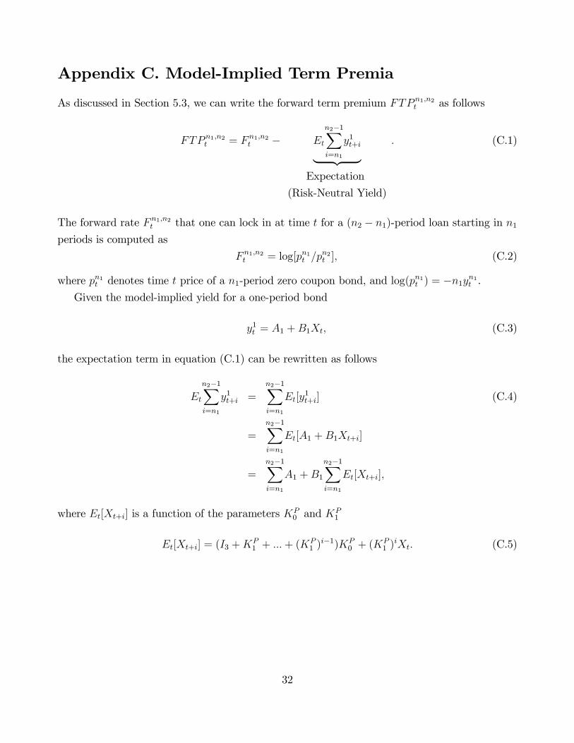
Appendix C. Model-Implied Term Premia

As discussed in Section 5.3, we can write the forward term premium FTP n1;n2t as follows

FTP n1;n2t = F n1;n2t � Et

n2�1Xi=n1

y1t+i| {z }Expectation

(Risk-Neutral Yield)

: (C.1)

The forward rate F n1;n2t that one can lock in at time t for a (n2 � n1)-period loan starting in n1periods is computed as

F n1;n2t = log[pn1t =pn2t ]; (C.2)

where pn1t denotes time t price of a n1-period zero coupon bond, and log(pn1t ) = �n1yn1t .

Given the model-implied yield for a one-period bond

y1t = A1 +B1Xt; (C.3)

the expectation term in equation (C.1) can be rewritten as follows

Et

n2�1Xi=n1

y1t+i =

n2�1Xi=n1

Et[y1t+i] (C.4)

=

n2�1Xi=n1

Et[A1 +B1Xt+i]

=

n2�1Xi=n1

A1 +B1

n2�1Xi=n1

Et[Xt+i];

where Et[Xt+i] is a function of the parameters KP0 and K

P1

Et[Xt+i] = (I3 +KP1 + :::+ (K

P1 )

i�1)KP0 + (K

P1 )

iXt: (C.5)

32

Appendix D: Latent Stochastic Volatility Models

Using the classi�cation of Dai and Singleton (2000), we focus on Aj(3) models with j = 1; 2 or

3 factors driving the conditional variance of the state variables, which are given by

dXt = (KP0� +K

P1�Xt)dt+ �

pStdW

Pt+1; (D.1)

dXt = (KQ0� +K

Q1�Xt)dt+ �

pStdW

Qt+1; (D.2)

rt = �0 + �1Xt; (D.3)

where W Pt+1 and W

Qt+1 are three-dimensional independent standard Brownian motions under

physical measure P and risk-neutral measure Q respectively, rt is the instantaneous spot interest

rate, and �St�0 is the conditional covariance matrix of Xt. St is a 3 � 3 diagonal matrix withthe ith diagonal element given by

[St]ii = �i + �0

iXt; (D.4)

where �i is a scalar, and �i is a 3 � 1 vector. � = [�1; �2; �3]0is a 3 � 1 vector. � = [�1; �2; �3]

is a 3� 3 matrix. We follow the Dai and Singleton identi�cation scheme to ensure the [St]ii arestrictly positive for all i.

The model-implied continuously compounded yields byt are given by (see Du¢ e and Kan,1996) byt = A(�Q) +B(�Q)Xt; (D.5)

where theN�1 vector A(�Q), and theN�3matrix B(�Q) are functions of the parameters underthe Q-dynamics, �Q = fKQ

0�; KQ1�; �0; �1;�; �; �g, through a set of Ricatti ordinary di¤erential

equations. Recall that N denotes the number of available yields in the term structure. We adopt

the essentially a¢ ne speci�cation for the price of risk, as in Du¤ee (2002).

The a¢ ne dynamic for Xt in equation (D.1) implies that the one-period ahead conditional

expectation of Xt under the P measure; bXt+�jt = constant + �eKP1�Xt; where � = 1=12. Thus

Xt follows a �rst order VAR when sampled monthly. Similarly, the a¢ ne dynamic in equation

(D.2) under the Q measure implies a �rst order VAR for Xt sampled at the monthly frequency.

For estimation based on the forecasting loss function in equation (2.3), we need the model�s

prediction of the k-period ahead n-maturity yield, based on parameter estimates at time t. This

is given by

bynt+kjt(�) = An(�Q) +Bn(�

Q) bXt+kjt (D.6)

= An(�Q) +Bn(�

Q)f(Xt; k;KP0 ; K

P1 );

33

where An(�Q) is the nth element of A(�Q), Bn(�Q) is the nth row of B(�Q), � = f�Q; KP0 ; K

P1 g,

and f is given by

f(Xt; k;KP0 ; K

P1 ) = (I3 +K

P1 + :::+ (K

P1 )

k�1)KP0 + (K

P1 )

kXt:

where KP0 and KP

1 are the parameters for the VAR(1) process of Xt under the P measure,

which can be mapped to KP0� and KP

1� respectively in equation (D.1) through the nonlinear

relations KP1 = e

�KP1� and KP

0 = KP0�

R �0esK

P1�ds. In particular, for small �, KP

0 � �KP0� and

KP1 � I3 +�KP

1�. We can view KP0 and K

P0�, and K

P1 and K

P1�, as interchangeable. Similarly,

KQ0 and K

Q0�, and K

Q1 and K

Q1� are interchangeable.

A three factor latent model can be expressed using a state-space representation. Using equa-

tion (D.1) and an Euler discretization, the state equation can be written as Xt+1 = KP0 +K

P1 Xt+

"Pt+1, where "Pt+1jt is assumed to be distributedN(0; �St�

0). The observed yield curve yt = byt+et isthe measurement equation, where byt is the model-implied yield as speci�ed in equation (D.5), andet is a vector of measurement errors that is assumed to be i:i:d: normal with diagonal covariance

matrix R. The estimates of the P -parameters, �P = fKP0 ; K

P1 g are related to the Q-parameters,

since the pricing model is required to �lter the latent factors Xt. We therefore need to esti-

mate the P - and Q-parameters simultaneously. We do this by applying the Kalman �lter to the

state-space representation. We estimate the parameters � = fKP0 ; K

P1 ; K

Q0 ; K

Q1 ; �0; �1;�; �; �g

and �lter the state variables Xt by minimizing the forecasting loss function, equation (2.3). We

compare the results obtained from the forecasting loss function with the estimation of the latent

stochastic volatility models based on the standard loss function equation (2.1).

When estimating models with latent factors, the numerical implementation is important

because of the existence of identi�cation problems. We follow the implementation of Hamilton

andWu (2012). We extract the �rst three principal components from the observed term structure

of yields, and normalize each principal component to have zero mean and unit variance. We

estimate the dynamics of the normalized �rst three principal components through OLS, and use

the OLS estimates of KP0 and K

P1 as initial values.

We obtain the initial values for �0 and �1 by regressing one-month yields on the normalized

principal components. To get the initial value for the Q parameters, we regress the observed

term structure of yields on the normalized principal components to get estimated loadings bAand bB. The Q parameters enter the loadings A(�Q) and B(�Q), which are de�ned recursively.Subsequently we obtain an initial guess for the Q parameters by minimizing the distances from

A(�Q) and B(�Q) to the estimated loadings bA and bB.With this set of initial values, we �nd � by optimizing the standard log likelihood function

34

using the fminsearch algorithm in MATLAB. We compute the 99% con�dence interval, [��;��],

for the converged values of �. Then we generate another 100 di¤erent sets of � from the uniform

distributions U [��;��]. We rank these di¤erent sets of � by the implied likelihood, and use the

top 10 ranked sets of � as initial values for another round of numerical search. We choose the

converged sets of � based on the likelihood, and form the new range of the parameter set using

the chosen sets of �. We continue generating di¤erent sets of initial values until they converge

to very similar values.

35

References

[1] Adrian, T., Crump, R. K., and Moench, E. (2013). Pricing the term structure with linear

regressions. Journal of Financial Economics, 110(1), 110-138.

[2] Ang, A., and Piazzesi, M. (2003). A no-arbitrage vector autoregression of term structure

dynamics with macroeconomic and latent variables. Journal of Monetary Economics, 50(4),

745-787.

[3] Ang, A., Piazzesi, M., and Wei, M. (2006). What does the yield curve tell us about GDP

growth?. Journal of Econometrics, 131(1), 359-403.

[4] Aït-Sahalia, Y., and Kimmel, R. L. (2010). Estimating a¢ ne multifactor term structure

models using closed-form likelihood expansions. Journal of Financial Economics, 98(1), 113-

144.

[5] Bauer, M. D., Rudebusch, G. D., and Wu, J. C. (2012). Correcting estimation bias in

dynamic term structure models. Journal of Business and Economic Statistics, 30(3), 454-

467.

[6] Bowsher, C. G., and Meeks, R. (2008). The dynamics of economic functions: modeling

and forecasting the yield curve. Journal of the American Statistical Association, 103(484),

1419-1437.

[7] Campbell, J. Y. and Cochrane, J. H. (1999). By force of habit: a consumption-based expla-

nation of aggregate stock market behavior. Journal of Political Economy, 107(2), 205�251.

[8] Chen, R. R., and Scott, L. (1992). Pricing interest rate options in a two-factor Cox-Ingersoll-

Ross model of the term structure. Review of Financial Studies, 5(4), 613-636.

[9] Christensen, J. H., Diebold, F. X., and Rudebusch, G. D. (2011). The a¢ ne arbitrage-free

class of Nelson�Siegel term structure models. Journal of Econometrics, 164(1), 4-20.

[10] Christo¤ersen, P. F., and Diebold, F. X. (1996). Further results on forecasting and model

selection under asymmetric loss. Journal of Applied Econometrics, 11(5), 561-571.

[11] Christo¤ersen, P. F., and Diebold, F. X. (1997). Optimal prediction under asymmetric loss.

Econometric Theory, 13(6), 808-817.

[12] Cieslak, A., and Povala, P. (2015). Expected returns in Treasury bonds. Review of Financial

Studies.

36

[13] Cochrane, J. H. (2005). Asset pricing. Princeton University Press.

[14] Cochrane, J. H., and Piazzesi, M. (2005). Bond risk premia. American Economic Review,

95(1), 138-160.

[15] Collin-Dufresne, P., Goldstein, R. S., and Jones, C. S. (2008). Identi�cation of maximal

a¢ ne term structure models. The Journal of Finance, 63(2), 743-795.

[16] Cooper, I., and Priestley, R. (2009). Time-varying risk premiums and the output gap. Review

of Financial Studies, 22(7), 2801-2833.

[17] Cox, D. R. (1961). Prediction by exponentially weighted moving averages and related meth-

ods. Journal of the Royal Statistical Society. Series B (Methodological), 414-422.

[18] Cox, J. C., Ingersoll Jr, J. E., and Ross, S. A. (1985). A theory of the term structure of

interest rates. Econometrica, 53(2), 385-408.

[19] Creal, D. D., and Wu, J. C. (2015). Estimation of a¢ ne term structure models with spanned

or unspanned stochastic volatility. Journal of Econometrics, 185(1), 60-81.

[20] Dai, Q., and Singleton, K. J. (2000). Speci�cation analysis of a¢ ne term structure models.

The Journal of Finance, 55(5), 1943-1978.

[21] Diebold, F. X. (2015). Comparing predictive accuracy, twenty years later: A personal per-

spective on the use and abuse of Diebold�Mariano tests. Journal of Business & Economic

Statistics, 33(1), 1-1.

[22] Diebold, F. X., and Li, C. (2006). Forecasting the term structure of government bond yields.

Journal of Econometrics, 130(2), 337-364.

[23] Diebold, F. X., and Mariano, R. (1995). Comparing predictive accuracy. Journal of Business

and Economic Statistics 13(3), 253-63.

[24] Diebold, F. X., and Shin, M. (2015). Assessing point forecast accuracy by stochastic loss

distance. Economics Letters, 130, 37-38.

[25] Diez de Los Rios, A. (2014). A new linear estimator for Gaussian dynamic term structure

models. Journal of Business and Economic Statistics, 33(2), 282-295.

[26] Du¤ee, G. R. (2002). Term premia and interest rate forecasts in a¢ ne models. The Journal

of Finance, 57(1), 405-443.

37

[27] Du¤ee, G. R. (2011a). Information in (and not in) the term structure. Review of Financial

Studies, 24(9), 2895-2934.

[28] Du¤ee, G. R. (2011b). Forecasting with the term structure: The role of no-arbitrage restric-

tions. Working Paper. Johns Hopkins University.

[29] Du¤ee, G. R., and Stanton, R. H. (2012). Estimation of dynamic term structure models.

The Quarterly Journal of Finance, 2(2).

[30] Du¢ e, D., and Kan, R. (1996). A yield-factor model of interest rates. Mathematical Finance,

6(4), 379-406.

[31] Egorov, A. V., Hong, Y., and Li, H. (2006). Validating forecasts of the joint probability

density of bond yields: Can a¢ ne models beat random walk? Journal of Econometrics,

135(1), 255-284.

[32] Elliott, G., Komunjer, I., and Timmermann, A. (2005). Estimation and testing of forecast

rationality under �exible loss. The Review of Economic Studies, 72(4), 1107-1125.

[33] Elliott, G., Komunjer, I., and Timmermann, A. (2008). Biases in macroeconomic forecasts:

irrationality or asymmetric loss? Journal of the European Economic Association, 6(1), 122-

157.

[34] Elliott, G., and Timmermann, A. (2008). Economic forecasting. Journal of Economic Liter-

ature, 46(1), 3-56.

[35] Engle, R. (1993). A comment on Hendry and Clements on the limitations of comparing

mean square forecast errors. Journal of Forecasting 12(8), 642-644.

[36] Gourieroux, C., Monfort, A., and Polimenis, V. (2006). A¢ ne models for credit risk analysis.

Journal of Financial Econometrics, 4(3), 494-530.

[37] Granger, C. W. (1993). On the limitations of comparing mean square forecast errors: Com-

ment. Journal of Forecasting, 12(8), 651-652.

[38] Gürkaynak, R. S., Sack, B., and Wright, J. H. (2007). The US Treasury yield curve: 1961

to the present. Journal of Monetary Economics, 54(8), 2291-2304.

[39] Hamilton, J. D., and Wu, J. C. (2012). Identi�cation and estimation of Gaussian a¢ ne term

structure models. Journal of Econometrics, 168(2), 315-331.

38

[40] Hamilton, J. D., and Wu, J. C. (2014). Testable implications of a¢ ne term structure models.

Journal of Econometrics, 178, 231-242.

[41] Harvey, C. R. (1989). Time-varying conditional covariances in tests of asset pricing models.

Journal of Financial Economics, 24(2), 289-317.

[42] Harvey, D., Leybourne, S., and Newbold, P. (1997). Testing the equality of prediction mean

squared errors. International Journal of Forecasting, 13(2), 281-291.

[43] Hong, Y., Li, H., and Zhao, F. (2004). Out-of-sample performance of discrete-time spot

interest rate models. Journal of Business & Economic Statistics, 22(4), 457-473.

[44] Joslin, S., and Le, A. (2013). Interest rate volatility and no-arbitrage a¢ ne term structure

models. Working Paper. University of Southern California.

[45] Joslin, S., Le, A., and Singleton, K. J. (2013). Why Gaussian macro-�nance term structure

models are (nearly) unconstrained factor-VARs. Journal of Financial Economics, 109(3),

604-622.

[46] Joslin, S., Priebsch, M., and Singleton, K. J. (2014). Risk premiums in dynamic term struc-

ture models with unspanned macro risks. The Journal of Finance, 69(3), 1197-1233.

[47] Joslin, S., Singleton, K. J., and Zhu, H. (2011). A new perspective on Gaussian dynamic

term structure models. Review of Financial Studies, 24(3), 926-970.

[48] Kang, I. B. (2003). Multi-period forecasting using di¤erent models for di¤erent horizons:

an application to US economic time series data. International Journal of Forecasting, 19(3),

387-400.

[49] Knez, P. J., Litterman, R., and Scheinkman, J. (1994). Explorations into factors explaining

money market returns. The Journal of Finance, 49(5), 1861-1882.

[50] Kim, D. H., and Orphanides, A. (2012). Term structure estimation with survey data on

interest rate forecasts. Journal of Financial and Quantitative Analysis, 47(01), 241-272.

[51] Le, A., Singleton, K. J., and Dai, Q. (2010). Discrete-time a¢ ne term structure models with

generalized market prices of risk. Review of Financial Studies, 23(5), 2184-2227.

[52] Lin, J. L., and Granger, C. W. (1994). Forecasting from non-linear models in practice.

Journal of Forecasting, 13(1), 1-9.

39

[53] Litterman, R. B., and Scheinkman, J. (1991). Common factors a¤ecting bond returns. The

Journal of Fixed Income, 1(1), 54-61.

[54] Liu, S.-I. (1996). Model selection for multiperiod forecasts. Biometrika, 83, 861-873.

[55] Longsta¤, F. A., and Schwartz, E. S. (1992). Interest rate volatility and the term structure:

A two-factor general equilibrium model. The Journal of Finance, 47(4), 1259-1282.

[56] Ludvigson, S. C., and Ng, S. (2009). Macro factors in bond risk premia. Review of Financial

Studies, 22(12), 5027-5067.

[57] Marcellino, M., Stock, J. H., and Watson, M. W. (2006). A comparison of direct and iterated

multistep AR methods for forecasting macroeconomic time series. Journal of Econometrics,

135(1), 499-526.

[58] Nelson, C. R., and Siegel, A. F. (1987). Parsimonious modeling of yield curves. Journal of

Business, 60, 473-489.

[59] Patton, A. J., and Timmermann, A. (2007a). Properties of optimal forecasts under asym-

metric loss and nonlinearity. Journal of Econometrics, 140(2), 884-918.

[60] Patton, A. J., and Timmermann, A. (2007b). Testing forecast optimality under unknown

loss. Journal of the American Statistical Association, 102(480), 1172-1184.

[61] Sarno, L., Schneider, P., and Wagner, C. (2014). The economic value of predicting bond

risk premia: Can anything beat the expectations hypothesis? Working Paper. University of

Lugano.

[62] Shin, M., and Zhong, M. (2013). Does realized volatility help bond yield density prediction?

Working Paper. University of Pennsylvania.

[63] Vasicek, O. (1977). An equilibrium characterization of the term structure. Journal of Finan-

cial Economics, 5(2), 177-188.

[64] Wachter, J. A. (2006). A consumption-based model of the term structure of interest rates.

Journal of Financial economics, 79(2), 365-399.

[65] Weiss, A. A. (1991). Multi-step estimation and forecasting in dynamic models. Journal of

Econometrics, 48(1), 135-149.

[66] Weiss, A. A. (1996). Estimating time series models using the relevant cost function. Journal

of Applied Econometrics, 11(5), 539-560.

40

Figure 1: State Variables for the JSZ Canonical Form with Standard Loss Function.

1954 1959 1964 1969 1974 1977 1984 1989 1994 1999 2004 20092012−0.1

0

0.1

0.2

0.3

0.4

Panel A: First Three Principal Components

PC1 PC2 PC3

3 6 12 24 36 48 60 120 240

−0.5

0

0.5

1Panel B: Loadings of the First Three Principal Components on the Yields

Yield Maturity

PC1 PC2 PC3

3 6 12 24 36 48 60 120 240

−0.5

0

0.5

1Panel C: Portfolio Weights of the First Three Principal Components

Yield Maturity

PC1 PC2 PC3

Notes to Figure: For the JSZ canonical form with standard loss function, Panel A shows thetime series of the first three principal components PC, Panel B shows the factor loadingsB(ΘQ) on the yield curve, and Panel C shows the portfolio weights W0.

Figure 2: Differences Between State Variables Using Forecasting and Standard Loss Functions.

1954 1964 1974 1984 1994 2004 2012-0.04

-0.02

0

0.02

1 Month Horizon

1954 1964 1974 1984 1994 2004 2012-0.04

-0.02

0

0.02

2 Month Horizon

1954 1964 1974 1984 1994 2004 2012-0.04

-0.02

0

0.02

3 Month Horizon

1954 1964 1974 1984 1994 2004 2012-0.04

-0.02

0

0.02

4 Month Horizon

1954 1964 1974 1984 1994 2004 2012-0.04

-0.02

0

0.02

5 Month Horizon

1954 1964 1974 1984 1994 2004 2012-0.04

-0.02

0

0.02

6 Month Horizon

1954 1964 1974 1984 1994 2004 2012-0.04

-0.02

0

0.02

9 Month Horizon

1954 1964 1974 1984 1994 2004 2012-0.04

-0.02

0

0.02

12 Month Horizon

Factor1 Factor2 Factor3

Notes to Figure: We plot the differences between the state variables from the JSZ canonicalform with forecasting loss function and variable portfolio weights and the state variables fromthe JSZ canonical form with standard loss function. The state variables are estimated usingthe entire sample. The panels represent the differences in the estimates for different forecasthorizons.

Figure 3: Differences Between Factor Loadings Using Forecasting and Standard Loss Functions.

3 6 12 24 36 48 60 120 240

-0.5

0

0.5

11 Month Horizon

3 6 12 24 36 48 60 120 240

-0.5

0

0.5

12 Month Horizon

3 6 12 24 36 48 60 120 240

-0.5

0

0.5

13 Month Horizon

3 6 12 24 36 48 60 120 240

-0.5

0

0.5

14 Month Horizon

3 6 12 24 36 48 60 120 240

-0.5

0

0.5

15 Month Horizon

3 6 12 24 36 48 60 120 240

-0.5

0

0.5

16 Month Horizon

Yield Maturity3 6 12 24 36 48 60 120 240

-0.5

0

0.5

19 Month Horizon

Yield Maturity3 6 12 24 36 48 60 120 240

-0.5

0

0.5

112 Month Horizon

Factor1 Factor2 Factor3

Notes to Figure: We plot the differences between the factor loadings from the JSZ canonicalform with forecasting loss function and variable portfolio weights and the factor loadings fromthe JSZ canonical form with standard loss function. The factor loadings are estimated usingthe entire sample. The panels represent the differences in the estimates for different forecasthorizons.

Figure 4: Differences Between Portfolio Weights Using Forecasting and Standard Loss Functions.

3 6 12 24 36 48 60 120 240-1

0

11 Month Horizon

3 6 12 24 36 48 60 120 240-1

0

12 Month Horizon

3 6 12 24 36 48 60 120 240-1

0

13 Month Horizon

3 6 12 24 36 48 60 120 240-1

0

14 Month Horizon

3 6 12 24 36 48 60 120 240-1

0

15 Month Horizon

3 6 12 24 36 48 60 120 240-1

0

16 Month Horizon

Yield Maturity3 6 12 24 36 48 60 120 240

-1

0

19 Month Horizon

Yield Maturity3 6 12 24 36 48 60 120 240

-1

0

112 Month Horizon

Factor1 Factor2 Factor3

Notes to Figure: We plot the differences between the variable portfolio weights from theJSZ canonical form with forecasting loss function and the fixed portfolio weights from theJSZ canonical form with standard loss function. The portfolio weights are estimated usingthe entire sample. The panels represent the differences in the estimates for different forecasthorizons.

Figure 5: Decomposing Forward Rates.

One-Month Forecast Horizon Twelve-Month Forecast Horizon

Term Premium Difference

1954 1964 1974 1984 1994 2004 20120

0.01

0.02

0.03

Term Premium Difference

1954 1964 1974 1984 1994 2004 20120

0.01

0.02

0.03

Differences Between Loss Functions

Risk-Neutral Yield

1954 1964 1974 1984 1994 2004 20120

0.05

0.1

Risk-Neutral Yield

1954 1964 1974 1984 1994 2004 20120

0.05

0.1

Term Premium

1954 1964 1974 1984 1994 2004 20120

0.05

0.1Term Premium

1954 1964 1974 1984 1994 2004 20120

0.05

0.1

Forecasting Loss Function Standard Loss Function

Notes to Figure: We plot model estimates of term premia and risk-neutral yields (the expec-tations component of yields) for five-to-ten-year forward rates. The highlighted line shows theestimates from the JSZ canonical form with standard loss function. The dotted line showsthe estimates from the JSZ canonical form with forecasting loss function and variable port-folio weights. The solid line in the bottom two panels represents the differences between theterm premia from the JSZ canonical form with forecasting loss function and variable portfolioweights and the term premia from the JSZ canonical form with standard loss function. Thepanels on the left plot results for the one-month forecast horizon, and the panels on the rightplot results for the twelve-month forecast horizon. The shaded areas indicate recessions asdefined by the National Bureau of Economic Research (NBER).

Table 1: Summary Statistics

Central Moments AutocorrelationMean St.Dev Skewness Kurtosis Lag 1 Lag 12 Lag 30

3 month yield 0.0450 0.0290 0.8938 4.3247 0.9773 0.7944 0.51976 month yield 0.0479 0.0305 0.8717 4.2283 0.9850 0.8126 0.53591 year yield 0.0516 0.0306 0.6980 3.6594 0.9857 0.8317 0.58912 year yield 0.0536 0.0301 0.6734 3.4957 0.9878 0.8509 0.64853 year yield 0.0554 0.0294 0.6703 3.4460 0.9884 0.8611 0.67824 year yield 0.0569 0.0288 0.6903 3.4142 0.9882 0.8655 0.70005 year yield 0.0579 0.0282 0.7270 3.3717 0.9890 0.8739 0.718310 year yield 0.0617 0.0275 0.9148 3.5853 0.9890 0.8739 0.718320 year yield 0.0638 0.0265 0.9158 3.5373 0.9930 0.8936 0.7724

Notes to Table: We present summary statistics for the data used in estimation. Wepresent the sample mean, standard deviation, skewness, kurtosis, and autocorrelations foreach of the yields. The yields are continuously compounded monthly zero-coupon bondyields. The sample period is from 1953:04 to 2012:12.

Table 2: Out-of-Sample RMSEs: JSZ Canonical Form

Panel A: Forecasting Loss FunctionForecast Horizon k 1 month 2 month 3 month 4 month 5 month 6 month 9 month 12 month

3 month yield 37.02 46.51 56.77 67.12 76.45 87.09 114.96 146.766 month yield 27.31 43.64 57.05 70.74 81.84 94.58 125.89 160.31

1 year yield 36.37 53.92 67.82 80.75 91.26 103.03 131.51 163.322 year yield 48.85 63.84 76.13 87.09 96.26 106.25 130.05 158.133 year yield 45.40 59.87 71.53 81.66 90.23 99.15 120.06 145.654 year yield 38.01 53.53 65.15 74.73 82.72 90.95 109.95 133.655 year yield 31.29 48.20 60.44 70.36 78.60 86.54 104.62 126.41

10 year yield 35.39 48.74 58.54 66.76 74.17 80.70 96.60 114.1720 year yield 50.51 57.97 64.86 70.28 76.01 80.68 92.52 105.21

Panel B: Standard Loss FunctionForecast Horizon k 1 month 2 month 3 month 4 month 5 month 6 month 9 month 12 month

3 month yield 38.72 55.31 69.90 80.40 91.57 103.00 136.41 162.376 month yield 33.68 52.77 70.13 84.76 98.56 111.71 146.05 174.08

1 year yield 37.51 59.02 78.09 94.16 108.31 121.03 153.24 179.912 year yield 39.83 63.66 82.94 98.76 112.23 124.11 152.92 177.253 year yield 37.95 60.60 78.53 93.15 105.56 116.32 142.01 164.414 year yield 34.56 55.80 72.41 85.65 96.97 106.86 130.12 150.985 year yield 32.00 52.34 68.19 80.92 91.77 101.07 122.68 142.36

10 year yield 32.62 49.44 61.88 72.43 81.54 89.17 107.30 124.7920 year yield 26.92 41.27 52.09 61.43 69.49 76.19 92.18 107.75

Panel C: RMSE RatioForecast Horizon k 1 month 2 month 3 month 4 month 5 month 6 month 9 month 12 month

3 month yield 0.96 0.84*** 0.81*** 0.83*** 0.83*** 0.85*** 0.84*** 0.90***6 month yield 0.81*** 0.83*** 0.81*** 0.83*** 0.83*** 0.85*** 0.86*** 0.92***

1 year yield 0.97 0.91*** 0.87*** 0.86*** 0.84*** 0.85*** 0.86*** 0.91***2 year yield 1.23*** 1.00 0.92*** 0.88*** 0.86*** 0.86*** 0.85*** 0.89***3 year yield 1.20*** 0.99 0.91*** 0.88*** 0.85*** 0.85*** 0.85*** 0.89***4 year yield 1.10*** 0.96** 0.90*** 0.87*** 0.85*** 0.85*** 0.84*** 0.89***5 year yield 0.98 0.92*** 0.89*** 0.87*** 0.86*** 0.86*** 0.85*** 0.89***

10 year yield 1.08** 0.99 0.95* 0.92*** 0.91*** 0.90*** 0.90*** 0.91***20 year yield 1.88*** 1.40*** 1.25*** 1.14*** 1.09*** 1.06* 1.00 0.98

Notes to Table: We present the out-of-sample RMSEs for the JSZ canonical form with forecasting loss function and standardloss function. Panel A reports on the JSZ canonical form with forecasting loss function and variable portfolio weights. At eachtime t and for each forecast horizon k, we estimate the model using data up to and including t, and forecast k periods ahead.Panel B reports on the JSZ canonical form with standard loss function and fixed portfolio weights. We estimate the modelusing data up to and including t at each month t, and forecast one to twelve months ahead. RMSEs are reported in basispoints. Panel C shows the ratios of the RMSEs in Panel A and Panel B. The statistical significance of the relative forecastingperformance is evaluated using the Diebold and Mariano (1995) test statistic computed with a serial correlation robust varianceand the small sample adjustment of Harvey, Leybourne, and Newbold (1997). The significance is denoted by *, ** and ***,corresponding to significance levels of 10%, 5% and 1% respectively.

Table 3: In-Sample RMSEs: JSZ Canonical Form

Panel A: Forecasting Loss FunctionForecast Horizon k 1 month 2 month 3 month 4 month 5 month 6 month 9 month 12 month

3 month yield 31.12 32.81 33.48 37.30 34.51 38.77 40.33 54.966 month yield 18.64 18.57 17.75 18.29 18.34 18.83 18.00 38.60

1 year yield 17.39 17.59 18.57 20.46 21.41 24.39 23.13 41.082 year yield 23.14 23.26 23.96 24.39 24.20 26.03 25.48 31.283 year yield 24.24 24.14 24.64 24.88 24.59 25.77 24.77 26.974 year yield 21.34 21.20 21.69 21.87 21.55 22.65 21.39 22.685 year yield 16.95 16.62 17.10 16.87 17.18 17.66 16.98 17.89

10 year yield 19.28 19.79 19.61 19.72 19.27 20.35 20.66 21.7520 year yield 34.89 35.31 35.20 35.62 35.41 36.46 38.09 41.61

Panel B: Standard Loss Function3 month yield 15.186 month yield 13.99

1 year yield 15.042 year yield 8.553 year yield 6.874 year yield 9.865 year yield 10.68

10 year yield 11.6220 year yield 11.54

Notes to Table: We present the in-sample RMSEs for the JSZ canonical form with forecasting loss function and variableportfolio weights (Panel A), and the JSZ canonical form with standard loss function and fixed portfolio weights (Panel B). Theestimates of the specification with forecasting loss function are forecast-horizon specific, so we report the in-sample RMSEs foreach forecast horizon. RMSEs are reported in basis points.

Table 4: Correlations Between State Variables and Principal Components

Principal Components PC1 PC2 PC3 PC4 PC5

1 Month HorizonFactor 1 1.0000 -0.0024 0.0066 -0.0029 -0.0014Factor 2 -0.0136 0.9999 0.0041 0.0015 0.0008Factor 3 -0.0386 0.0653 0.0114 0.9971 -0.0001

2 Month HorizonFactor 1 1.0000 -0.0042 0.0082 -0.0060 -0.0032Factor 2 -0.0105 0.9999 0.0083 0.0008 -0.0001Factor 3 -0.0668 0.0564 -0.0297 0.9959 -0.0059

3 Month HorizonFactor 1 1.0000 -0.0087 0.0138 -0.0090 -0.0046Factor 2 0.0043 0.9999 0.0138 0.0002 -0.0008Factor 3 -0.1452 0.1145 -0.0495 0.9823 -0.0180

4 Month HorizonFactor 1 1.0000 -0.0088 0.0154 -0.0135 -0.0078Factor 2 0.0459 0.9987 0.0162 -0.0012 -0.0012Factor 3 -0.2001 0.1854 -0.0728 0.9611 -0.0081

5 Month HorizonFactor 1 0.9999 -0.0146 0.0182 -0.0164 -0.0093Factor 2 0.0622 0.9977 0.0200 -0.0015 -0.0025Factor 3 -0.1749 0.3172 -0.0499 0.9324 -0.0165

6 Month HorizonFactor 1 0.9999 -0.0204 0.0237 -0.0184 -0.0109Factor 2 0.0751 0.9967 0.0140 -0.0017 -0.0027Factor 3 -0.2396 0.2713 -0.0696 0.9324 -0.0357

9 Month HorizonFactor 1 0.9999 -0.0189 0.0272 -0.0289 -0.0151Factor 2 0.0773 0.9964 0.0186 -0.0004 -0.0029Factor 3 -0.1679 0.4725 -0.1468 0.8531 -0.0220

12 Month HorizonFactor 1 0.9998 -0.0234 0.0379 -0.0401 -0.0213Factor 2 0.2431 0.9677 0.0542 0.0022 -0.0011Factor 3 -0.2270 0.4452 -0.1344 0.8596 -0.0147

Notes to Table: We present the correlations between the state variables from the JSZ canonical form withforecasting loss function and the first five principal components (PC) of the yield curve. The state variablesare estimated using the entire sample. The estimates are forecast-horizon specific.

Table

5:Para

meterEstim

ates:

JSZ

CanonicalForm

PanelA:Foreca

stingLoss

Function

P-D

ynam

ics

Q-D

ynam

ics

ForecastHorizon

KP 0

KP 1

Eigenvalues

KQ 0

KQ 1

Eigenvalues

ΣΣ

′×

1e4

1mon

th-0.0015

0.9941

0.0551

-1.0073

0.9949

-0.0040

1.0292

0.0723

-1.9989

0.9991

0.9618

0.2112

0.0065

0.0018

0.0018

0.9328

0.5121

0.9417

0.0043

-0.0330

0.9735

2.1475

0.9341

0.2112

0.2351

0.0306

-0.0008

0.0004

0.0094

0.4795

0.4698

-0.0017

0.0157

-0.0148

0.0019

0.0714

0.0065

0.0306

0.0421

2mon

th-0.0015

0.9938

0.0551

-0.9093

0.9947

-0.0038

1.0281

0.0735

-1.9313

0.9991

0.9578

0.2122

0.0072

0.0018

0.0018

0.9336

0.5120

0.9438

0.0041

-0.0319

0.9722

2.0793

0.9339

0.2122

0.2316

0.0298

-0.0008

0.0004

0.0094

0.5334

0.5223

-0.0016

0.0152

-0.0142

0.0338

0.1010

0.0072

0.0298

0.0417

3mon

th-0.0014

0.9941

0.0551

-0.9144

0.9950

-0.0040

1.0298

0.0717

-2.0402

0.9991

0.9505

0.2090

0.0034

0.0018

0.0018

0.9327

0.5128

0.9429

0.0043

-0.0336

0.9741

2.1891

0.9340

0.2090

0.2316

0.0285

-0.0008

0.0004

0.0094

0.5317

0.5207

-0.0017

0.0159

-0.0150

-0.0139

0.0568

0.0034

0.0285

0.0426

4mon

th-0.0014

0.9938

0.0547

-1.0049

0.9946

-0.0039

1.0298

0.0720

-2.0462

0.9991

1.0043

0.2197

0.0199

0.0018

0.0018

0.9314

0.5031

0.9399

0.0042

-0.0337

0.9740

2.1917

0.9337

0.2197

0.2183

0.0294

-0.0009

0.0004

0.0096

0.4578

0.4485

-0.0017

0.0160

-0.0150

-0.0142

0.0567

0.0199

0.0294

0.0448

5mon

th-0.0014

0.9934

0.0566

-1.0069

0.9942

-0.0039

1.0293

0.0726

-2.0114

0.9993

0.9647

0.2175

0.0020

0.0018

0.0019

0.9266

0.5078

0.9356

0.0042

-0.0331

0.9733

2.1611

0.9341

0.2175

0.2299

0.0220

-0.0008

0.0003

0.0093

0.4835

0.4737

-0.0016

0.0157

-0.0145

0.0013

0.0705

0.0020

0.0220

0.0445

6mon

th-0.0013

0.9938

0.0559

-1.0066

0.9945

-0.0038

1.0293

0.0727

-2.0201

0.9992

0.9778

0.2196

0.0022

0.0018

0.0019

0.9290

0.5099

0.9382

0.0041

-0.0331

0.9732

2.1647

0.9337

0.2196

0.2241

0.0213

-0.0008

0.0004

0.0094

0.4907

0.4807

-0.0016

0.0157

-0.0145

0.0013

0.0708

0.0022

0.0213

0.0469

9mon

th-0.0013

0.9934

0.0539

-1.1175

0.9937

-0.0038

1.0293

0.0726

-2.0318

0.9991

1.0363

0.2149

0.0021

0.0018

0.0017

0.9314

0.5117

0.9426

0.0041

-0.0331

0.9734

2.1703

0.9347

0.2149

0.2050

0.0124

-0.0008

0.0004

0.0095

0.5490

0.5375

-0.0016

0.0157

-0.0142

0.0007

0.0696

0.0021

0.0124

0.0436

12mon

th-0.0012

0.9933

0.0529

-1.1491

0.9935

-0.0038

1.0299

0.0712

-2.0807

0.9992

1.0113

0.2024

0.0011

0.0017

0.0019

0.9286

0.4964

0.9401

0.0041

-0.0339

0.9736

2.2265

0.9331

0.2024

0.2049

0.0131

-0.0008

0.0004

0.0097

0.5545

0.5428

-0.0016

0.0160

-0.0146

-0.0153

0.0558

0.0011

0.0131

0.0417

PanelB:Standard

Loss

Function

P-D

ynam

ics

Q-D

ynam

ics

KP 0

KP 1

Eigenvalues

KQ 0

KQ 1

Eigenvalues

ΣΣ

′×

1e4

-0.0021

0.9940

0.0549

0.3129

0.9948

0.0004

1.0052

0.1039

-0.2569

1.0000

0.9893

0.2297

0.0513

0.0004

0.0017

0.9337

0.1538

0.9274

-0.0003

-0.0073

0.9370

0.2717

0.9648

0.2297

0.2544

0.0238

0.0012

-0.0002

-0.0042

0.8084

0.8139

0.0003

0.0042

0.0136

0.8685

0.8458

0.0513

0.0238

0.1203

Notes

toTable:WepresenttheestimatedP-an

dQ-parametersgoverningthestatevariab

lesin

theJSZ

canon

ical

form

withforecastingloss

functionan

dstan

dardloss

function.Theparametersareestimatedusingtheentire

sample.Panel

Areports

ontheJSZcanon

icalform

withforecastingloss

functionan

dvariab

leportfolio

weigh

ts.These

estimatesareforecast-horizon

specific.

Panel

BreportsontheJSZcanonicalform

withstandardloss

function.Weconduct

likelihoodratiotestson

theeigenvalues

estimated

from

differentloss

functions.

Theeigenvalues

show

nin

boldface

inPan

elA

are

sign

ificantlydifferentfrom

thecorrespon

dingeigenvalues

inPan

elB.

Table 6: Out-of-Sample RMSEs: AFNS

Panel A: Forecasting Loss FunctionForecast Horizon k 1 month 2 month 3 month 4 month 5 month 6 month 9 month 12 month

3 month yield 36.12 46.23 56.23 67.45 79.12 88.45 118.35 142.126 month yield 27.68 43.48 55.12 67.29 78.09 89.13 121.22 150.24

1 year yield 36.39 51.91 65.33 76.87 86.87 98.15 124.90 152.972 year yield 45.85 60.75 72.38 82.62 90.60 100.90 122.71 146.883 year yield 42.29 57.20 68.23 77.77 85.22 94.25 113.45 134.924 year yield 36.45 51.87 62.90 71.96 79.13 86.94 104.56 123.895 year yield 30.57 46.72 58.58 67.94 75.61 82.73 99.72 117.36

10 year yield 38.30 54.53 59.76 65.39 73.64 79.09 95.46 106.8620 year yield 51.13 60.13 68.06 75.18 79.50 84.24 93.32 105.71

Panel B: Standard Loss FunctionForecast Horizon k 1 month 2 month 3 month 4 month 5 month 6 month 9 month 12 month

3 month yield 40.49 57.84 73.01 84.12 95.69 107.43 141.22 167.426 month yield 33.48 52.14 69.17 83.55 97.18 110.22 144.37 172.31

1 year yield 37.09 56.92 75.04 90.40 104.03 116.35 148.01 174.432 year yield 38.15 61.79 80.97 96.67 110.02 121.83 150.57 174.873 year yield 38.43 61.33 79.48 94.27 106.82 117.69 143.54 166.014 year yield 36.37 57.97 74.88 88.42 99.99 110.08 133.60 154.585 year yield 34.98 55.50 71.56 84.56 95.65 105.14 127.03 146.83

10 year yield 34.24 51.02 63.49 74.06 83.19 90.87 109.12 126.7020 year yield 28.18 41.00 50.92 59.64 67.20 73.49 88.64 103.57

Panel C: RMSE RatioForecast Horizon k 1 month 2 month 3 month 4 month 5 month 6 month 9 month 12 month

3 month yield 0.89*** 0.80** 0.77*** 0.80 0.83*** 0.82*** 0.84*** 0.85***6 month yield 0.83*** 0.83*** 0.80*** 0.81*** 0.80*** 0.81*** 0.84*** 0.87***

1 year yield 0.98*** 0.91*** 0.87*** 0.85*** 0.84*** 0.84** 0.84** 0.88***2 year yield 1.20** 0.98** 0.89** 0.85*** 0.82*** 0.83*** 0.81*** 0.84***3 year yield 1.10*** 0.93*** 0.86** 0.83** 0.80* 0.80*** 0.79** 0.81***4 year yield 1.00 0.89*** 0.84*** 0.81*** 0.79** 0.79* 0.78*** 0.80**5 year yield 0.87** 0.84*** 0.82*** 0.80** 0.79** 0.79*** 0.79*** 0.80**

10 year yield 1.12*** 1.07*** 0.94*** 0.88*** 0.89*** 0.87*** 0.87*** 0.84***20 year yield 1.81** 1.47*** 1.34* 1.26** 1.18*** 1.15*** 1.05*** 1.02***

Notes to Table: We present the out-of-sample RMSEs for the maximally flexible specification of the Gaussian AFNS modelwith forecasting loss function and standard loss function. Panel A reports on the AFNS model with forecasting loss function.At each time t and for each forecast horizon k, we estimate the model using data up to and including t, and forecast k periodsahead. Panel B reports on the AFNS model with standard loss function. We estimate the model using data up to and includingt at each month t, and forecast one to twelve months ahead. RMSEs are reported in basis points. Panel C shows the ratios ofthe RMSEs in Panel A and Panel B. The statistical significance of the relative forecasting performance is evaluated using theDiebold and Mariano (1995) test statistic computed with a serial correlation robust variance and the small sample adjustmentof Harvey, Leybourne, and Newbold (1997). The significance is denoted by *, ** and ***, corresponding to significance levelsof 10%, 5% and 1% respectively.

Table 7: Out-of-Sample RMSE Ratios: Stochastic Volatility Models

Panel A: A1(3) with Latent FactorsForecast Horizon 1 month 2 month 3 month 4 month 5 month 6 month 9 month 12 month

3 month yield 0.99* 0.98* 1.00* 0.98** 0.95** 0.93** 0.89** 0.84***6 month yield 1.05 0.97* 0.99* 0.98** 0.96** 0.94** 0.84* 0.92***

1 year yield 1.01 0.98 0.98* 0.93** 0.95** 0.93** 0.91*** 0.88***2 year yield 1.23* 0.94* 0.95* 0.92** 0.90*** 0.88*** 0.82*** 0.83***3 year yield 1.18 0.91** 0.91** 0.88*** 0.86*** 0.85*** 0.79*** 0.80***4 year yield 1.07* 0.90*** 0.89** 0.84** 0.83*** 0.81*** 0.79*** 0.76***5 year yield 0.88** 0.88* 0.90** 0.88** 0.84*** 0.83*** 0.76*** 0.76***

10 year yield 0.97** 0.89* 0.89* 0.90** 0.83** 0.83** 0.76*** 0.72***20 year yield 1.83** 1.33 1.12 1.00 0.92 0.86* 0.78*** 0.76***

Panel B: A2(3) with Latent FactorsForecast Horizon 1 month 2 month 3 month 4 month 5 month 6 month 9 month 12 month

3 month yield 0.99 1.00 0.99** 0.95*** 0.93*** 0.90*** 0.85*** 0.79***6 month yield 1.05* 0.98** 1.00* 0.96*** 0.93*** 0.90*** 0.79*** 0.86***

1 year yield 0.99 0.96** 0.97** 0.95*** 0.92*** 0.94*** 0.92*** 0.88***2 year yield 1.21 0.86* 0.96*** 0.95*** 0.94*** 0.92*** 0.83*** 0.84***3 year yield 1.14 0.82*** 0.91*** 0.89*** 0.89*** 0.87*** 0.80*** 0.81***4 year yield 1.01** 0.83** 0.88*** 0.84*** 0.84*** 0.82*** 0.80*** 0.74***5 year yield 0.94* 0.85** 0.92*** 0.92*** 0.87*** 0.86*** 0.76*** 0.77***

10 year yield 0.93** 0.84* 0.89** 0.95*** 0.84*** 0.85*** 0.77*** 0.71***20 year yield 1.77** 1.25 1.05 0.93 0.85* 0.79* 0.74*** 0.79***

Panel C: A3(3) with Latent FactorsForecast Horizon 1 month 2 month 3 month 4 month 5 month 6 month 9 month 12 month

3 month yield 0.99** 0.99*** 0.96*** 0.96*** 0.93*** 0.91*** 0.86*** 0.80***6 month yield 1.04*** 0.99*** 1.00 0.97*** 0.93*** 0.91** 0.79*** 0.87***

1 year yield 1.00* 0.97*** 0.99*** 0.98*** 0.94*** 0.95*** 0.96*** 0.89***2 year yield 1.20 0.86*** 0.96*** 0.96*** 0.95*** 0.93*** 0.83*** 0.84***3 year yield 1.14** 0.82*** 0.91*** 0.90*** 0.89*** 0.87*** 0.81*** 0.82***4 year yield 1.02** 0.83*** 0.88*** 0.85*** 0.85*** 0.82*** 0.81*** 0.75***5 year yield 0.93*** 0.85*** 0.93*** 0.92*** 0.88*** 0.87*** 0.77*** 0.78***

10 year yield 0.94** 0.84*** 0.89*** 0.96*** 0.85*** 0.86*** 0.78*** 0.72***20 year yield 1.62*** 1.21*** 1.03 0.91** 0.83*** 0.77*** 0.75*** 0.81***

Notes to Table: We present the out-of-sample RMSE ratios for the stochastic volatility models with forecasting loss functionand standard loss function. Panel A reports on the A1(3) model, Panel B reports on the A2(3) model, and Panel C reportson the A3(3) model. For the forecasting loss function, at each time t and for each forecast horizon k, we estimate the modelsusing data up to and including t, and forecast k periods ahead. For the standard loss function, we estimate the modelsusing data up to and including t at each month t, and forecast one to twelve months ahead. The statistical significance ofthe relative forecasting performance is evaluated using the Diebold and Mariano (1995) test statistic computed with a serialcorrelation robust variance and the small sample adjustment of Harvey, Leybourne, and Newbold (1997). The significance isdenoted by *, ** and ***, corresponding to significance levels of 10%, 5% and 1% respectively.

Table 8: Out-of-Sample MAEs: JSZ Canonical Form

Panel A: Forecasting Loss FunctionForecast Horizon k 1 month 2 month 3 month 4 month 5 month 6 month 9 month 12 month

3 month yield 26.77 30.31 36.95 45.64 55.85 66.85 95.06 119.686 month yield 17.80 28.90 38.82 50.46 62.78 75.30 104.70 129.76

1 year yield 26.96 41.60 52.12 62.80 74.13 85.44 111.76 135.702 year yield 36.82 49.82 60.10 70.03 79.83 89.08 111.90 132.783 year yield 34.33 47.25 56.60 66.07 74.55 82.95 103.16 122.354 year yield 29.01 42.93 51.96 60.00 66.92 74.74 92.92 111.325 year yield 24.81 39.04 48.44 56.61 63.01 70.11 85.99 103.78

10 year yield 27.98 38.22 46.33 52.64 58.40 63.40 74.86 88.1620 year yield 41.36 48.18 52.95 56.84 60.64 64.10 71.78 81.17

Panel B: Standard Loss FunctionForecast Horizon k 1 month 2 month 3 month 4 month 5 month 6 month 9 month 12 month

3 month yield 26.62 38.94 50.45 60.44 71.37 81.41 109.79 131.296 month yield 24.41 39.89 53.84 66.38 78.76 90.22 118.78 140.71

1 year yield 29.20 46.52 62.23 75.78 88.55 99.91 125.80 146.252 year yield 31.94 50.90 66.51 80.31 92.32 102.68 126.89 146.243 year yield 30.42 48.51 62.85 75.72 86.91 96.88 119.29 137.174 year yield 27.37 44.30 57.55 68.97 79.33 88.91 110.18 126.745 year yield 25.49 41.68 54.09 64.93 74.74 84.12 104.19 119.86

10 year yield 25.65 38.72 48.91 58.02 65.95 72.67 89.15 102.8020 year yield 20.91 32.15 40.82 48.58 55.16 60.30 72.45 84.56

Panel C: MAE RatioForecast Horizon k 1 month 2 month 3 month 4 month 5 month 6 month 9 month 12 month

3 month yield 1.01 0.78*** 0.73*** 0.76*** 0.78*** 0.82*** 0.87*** 0.91***6 month yield 0.73*** 0.72*** 0.72*** 0.76*** 0.80*** 0.83*** 0.88*** 0.92***

1 year yield 0.92* 0.89*** 0.84*** 0.83*** 0.84*** 0.86*** 0.89*** 0.93***2 year yield 1.15 0.98 0.90*** 0.87*** 0.86*** 0.87*** 0.88*** 0.91***3 year yield 1.13** 0.97*** 0.90*** 0.87*** 0.86*** 0.86*** 0.86*** 0.89***4 year yield 1.06** 0.97* 0.90*** 0.87*** 0.84*** 0.84*** 0.84*** 0.88***5 year yield 0.97 0.94** 0.90*** 0.87*** 0.84*** 0.83*** 0.83*** 0.87***

10 year yield 1.09* 0.99 0.95 0.91** 0.89*** 0.87*** 0.84*** 0.86***20 year yield 1.98*** 1.50* 1.30** 1.17*** 1.10** 1.06 0.99 0.96*

Notes to Table: We present the out-of-sample MAEs for the JSZ canonical form with forecasting loss function and standardloss function. Panel A reports on the JSZ canonical form with forecasting loss function and variable portfolio weights. At eachtime t and for each forecast horizon k, we estimate the model using data up to and including t, and forecast k periods ahead.Panel B reports on the JSZ canonical form with standard loss function and fixed portfolio weights. We estimate the model usingdata up to and including t at each month t, and forecast one to twelve months ahead. MAEs are reported in basis points. PanelC shows the ratios of the MAEs in Panel A and Panel B. The statistical significance of the relative forecasting performance isevaluated using the Diebold and Mariano (1995) test statistic computed with a serial correlation robust variance and the smallsample adjustment of Harvey, Leybourne, and Newbold (1997). The significance is denoted by *, ** and ***, corresponding tosignificance levels of 10%, 5% and 1% respectively.

Table A1: Out-of-Sample RMSEs: A0(3) with Latent Factors

Panel A: Forecasting Loss FunctionForecast Horizon k 1 month 2 month 3 month 4 month 5 month 6 month 9 month 12 month

3 month yield 39.24 56.64 70.37 80.35 90.75 101.65 133.55 158.006 month yield 34.18 54.44 71.25 85.20 98.20 110.87 136.98 180.50

1 year yield 38.60 61.01 79.85 94.82 107.94 119.97 154.49 182.172 year yield 51.21 64.62 83.59 97.54 110.05 121.12 145.67 177.113 year yield 47.40 60.41 77.75 90.06 101.70 111.63 134.90 164.274 year yield 39.44 55.08 70.79 81.39 92.10 101.11 125.24 147.935 year yield 31.38 51.20 67.98 80.18 89.40 98.91 117.93 143.79

10 year yield 38.75 50.39 64.41 77.58 83.66 92.91 111.43 130.0220 year yield 43.11 57.40 65.76 73.09 78.31 81.67 94.18 107.69

Panel B: Standard Loss FunctionForecast Horizon k 1 month 2 month 3 month 4 month 5 month 6 month 9 month 12 month

3 month yield 42.43 57.80 73.42 88.17 104.39 121.31 150.07 165.456 month yield 36.97 56.15 70.62 86.27 102.28 120.48 152.18 187.41

1 year yield 38.95 60.58 80.87 96.05 109.16 122.05 157.64 188.162 year yield 41.28 65.69 83.41 98.41 112.67 128.05 153.59 189.393 year yield 38.79 62.79 77.24 93.07 110.19 126.17 154.13 178.944 year yield 35.39 58.78 73.27 89.29 104.76 119.57 132.66 165.835 year yield 34.09 53.12 70.81 86.26 101.18 115.26 140.62 162.65

10 year yield 33.40 50.65 63.46 77.44 89.47 101.59 136.72 155.5020 year yield 31.59 44.73 59.00 72.21 85.31 97.55 121.19 134.25

Panel C: RMSE RatioForecast Horizon k 1 month 2 month 3 month 4 month 5 month 6 month 9 month 12 month

3 month yield 0.92 0.98* 0.96*** 0.91*** 0.87*** 0.84*** 0.89*** 0.95***6 month yield 0.92* 0.97** 1.01*** 0.99*** 0.96*** 0.92*** 0.90** 0.96***

1 year yield 0.99 1.01* 0.99*** 0.99*** 0.99*** 0.98*** 0.98*** 0.97***2 year yield 1.24 0.98 1.00* 0.99*** 0.98*** 0.95*** 0.95*** 0.94***3 year yield 1.22 0.96* 1.01*** 0.97*** 0.92*** 0.88*** 0.88*** 0.92***4 year yield 1.11 0.94** 0.97*** 0.91*** 0.88*** 0.85*** 0.94*** 0.89***5 year yield 0.92* 0.96*** 0.96*** 0.93*** 0.88*** 0.86*** 0.84*** 0.88***

10 year yield 1.16 0.99* 1.01*** 1.00 0.94*** 0.91*** 0.82*** 0.84***20 year yield 1.36*** 1.28 1.11 1.01 0.92 0.84** 0.78*** 0.80***

Notes to Table: We present the out-of-sample RMSEs for the A0(3) latent model with forecasting loss function and standardloss function. Panel A reports on the A0(3) model with forecasting loss function. At each time t and for each forecast horizonk, we estimate the model using data up to and including t, and forecast k periods ahead. Panel B reports on the A0(3) modelwith standard loss function. We estimate the model using data up to and including t at each month t, and forecast one to twelvemonths ahead. RMSEs are reported in basis points. Panel C shows the ratios of the RMSEs in Panel A and Panel B. Thestatistical significance of the relative forecasting performance is evaluated using the Diebold and Mariano (1995) test statisticcomputed with a serial correlation robust variance and the small sample adjustment of Harvey, Leybourne, and Newbold (1997).The significance is denoted by *, ** and ***, corresponding to significance levels of 10%, 5% and 1% respectively.

Table A2: In-Sample RMSEs: AFNS

Panel A: Forecasting Loss FunctionForecast Horizon k 1 month 2 month 3 month 4 month 5 month 6 month 9 month 12 month

3 month yield 36.28 39.04 41.13 43.20 50.28 50.23 50.01 47.616 month yield 21.60 23.89 25.21 26.38 20.13 20.11 19.97 28.36

1 year yield 18.35 19.43 20.13 20.80 18.95 18.95 19.01 22.722 year yield 28.06 31.98 34.55 36.93 28.91 28.86 28.72 41.563 year yield 27.26 29.89 31.80 33.64 30.38 30.32 30.07 37.014 year yield 22.68 24.06 25.07 26.06 28.74 28.70 28.46 27.735 year yield 16.19 16.63 16.97 17.31 26.66 26.64 26.48 17.71

10 year yield 22.26 24.75 26.29 27.70 24.24 24.40 24.67 30.2420 year yield 40.99 43.34 45.15 46.95 75.70 75.70 75.37 50.15

Panel B: Standard Loss Function3 month yield 18.566 month yield 15.87

1 year yield 19.902 year yield 10.813 year yield 9.184 year yield 10.275 year yield 11.64

10 year yield 12.6720 year yield 10.00

Notes to Table: We present the in-sample RMSEs for the maximally flexible specification of the AFNS model with forecastingloss function (Panel A) and standard loss function (Panel B). The estimates of the specification with forecasting loss functionare forecast-horizon specific, so we report the in-sample RMSEs for each forecast horizon. RMSEs are reported in basis points.

Table A3: In-Sample RMSEs: AFNS with Independent Factors

Panel A: Forecasting Loss FunctionForecast Horizon k 1 month 2 month 3 month 4 month 5 month 6 month 9 month 12 month

3 month yield 43.91 46.78 53.67 53.56 67.65 63.44 63.29 62.976 month yield 24.60 24.56 24.50 24.43 22.79 24.36 24.22 23.96

1 year yield 24.60 24.62 24.65 24.68 18.64 24.73 24.85 25.012 year yield 35.77 35.69 35.63 35.56 37.72 35.48 35.41 35.273 year yield 38.88 38.75 38.64 38.52 35.62 38.37 38.18 37.844 year yield 37.69 37.57 37.46 37.33 27.68 37.18 36.94 36.525 year yield 33.55 33.51 33.43 33.36 19.48 33.29 33.09 32.69

10 year yield 29.08 29.76 30.16 30.63 26.83 31.38 31.75 31.9620 year yield 51.45 51.40 61.24 61.11 71.69 81.00 85.52 89.72

Panel B: Standard Loss Function3 month yield 23.806 month yield 15.72

1 year yield 27.612 year yield 11.383 year yield 7.594 year yield 12.955 year yield 18.03

10 year yield 20.2320 year yield 24.45

Notes to Table: We present the in-sample RMSEs for the independent-factor AFNS model with forecasting loss function (PanelA) and standard loss function (Panel B). The estimates of the specification with forecasting loss function are forecast-horizonspecific, so we report the in-sample RMSEs for each forecast horizon. RMSEs are reported in basis points.

Table A4: In-Sample RMSEs: Stochastic Volatility Models

Panel A: A1(3) with Latent Factors

Forecasting Loss Function Standard Loss FunctionForecast Horizon k 1 month 2 month 3 month 4 month 5 month 6 month 9 month 12 month

3 month yield 35.30 43.35 44.36 38.47 42.75 48.67 54.68 58.54 18.216 month yield 21.58 20.05 20.48 20.74 21.27 23.74 30.34 41.92 15.66

1 year yield 20.17 22.44 22.14 23.33 26.54 24.24 35.47 46.59 17.262 year yield 26.10 27.69 27.44 27.63 28.70 29.08 32.17 35.89 11.013 year yield 27.68 28.60 28.45 28.41 28.94 30.00 30.10 30.88 7.834 year yield 24.63 25.14 25.23 24.94 25.43 27.42 26.10 25.83 10.435 year yield 20.20 19.84 19.81 19.90 20.36 25.05 20.15 20.11 12.12

10 year yield 22.49 21.82 21.95 21.74 21.83 28.08 24.15 25.59 12.8220 year yield 40.08 39.98 39.50 39.63 40.78 47.67 43.23 46.95 15.34

Panel B: A2(3) with Latent Factors

Forecasting Loss Function Standard Loss FunctionForecast Horizon k 1 month 2 month 3 month 4 month 5 month 6 month 9 month 12 month

3 month yield 34.96 35.61 37.63 40.04 64.62 44.21 51.89 44.88 18.186 month yield 21.32 20.42 21.26 20.46 25.42 23.03 26.15 29.86 16.77

1 year yield 19.69 21.39 21.48 22.10 26.29 23.45 31.00 37.55 18.512 year yield 26.59 27.12 27.09 27.49 28.61 28.46 29.64 32.18 14.073 year yield 27.98 28.24 28.35 28.32 29.50 29.30 28.57 29.69 12.574 year yield 24.78 24.91 25.22 24.84 26.68 26.35 24.97 25.99 11.795 year yield 19.85 20.21 21.40 19.91 21.15 23.22 19.39 22.15 10.77

10 year yield 21.77 22.03 23.27 22.02 23.59 25.44 23.26 26.69 11.7420 year yield 39.55 40.23 40.48 40.13 39.55 43.39 42.94 48.83 16.42

Panel C: A3(3) with Latent Factors

Forecasting Loss Function Standard Loss FunctionForecast Horizon k 1 month 2 month 3 month 4 month 5 month 6 month 9 month 12 month

3 month yield 35.28 35.44 40.43 36.05 57.04 38.87 78.56 54.56 19.296 month yield 19.27 18.96 21.85 20.48 23.21 19.84 40.10 33.59 17.79

1 year yield 19.61 21.35 20.92 20.82 24.40 23.11 37.90 38.47 19.512 year yield 25.52 26.60 27.38 25.99 26.88 26.88 31.64 32.43 14.923 year yield 26.78 27.45 28.55 26.92 27.37 27.61 29.77 29.68 13.344 year yield 23.68 24.14 25.49 23.69 24.20 24.95 26.26 25.70 12.505 year yield 18.79 19.60 22.00 18.93 18.86 22.28 21.06 20.51 11.42

10 year yield 21.01 21.07 22.22 20.90 21.74 24.94 22.61 22.22 11.3920 year yield 37.98 38.52 38.88 38.09 38.92 41.96 41.11 41.27 18.99

Notes to Table: We present the in-sample RMSEs for the A1(3), A2(3) and A3(3) stochastic volatility models with forecasting loss function and standard lossfunction. For the models with forecasting loss function, the estimates are forecast-horizon specific, so we report the in-sample RMSEs for each forecast horizon.RMSEs are reported in basis points.

Table A5: Out-of-Sample RMSEs: AFNS Model with Independent Factors

Panel A: Forecasting Loss FunctionForecast Horizon k 1 month 2 month 3 month 4 month 5 month 6 month 9 month 12 month

3 month yield 36.47 45.70 57.08 66.56 82.69 88.66 117.24 138.266 month yield 27.19 41.32 53.54 65.12 73.99 85.41 114.56 139.89

1 year yield 35.63 48.71 61.25 71.07 80.26 90.77 115.08 138.852 year yield 42.08 56.41 66.99 76.17 82.68 93.04 112.24 132.023 year yield 38.46 53.33 63.36 72.01 78.07 86.98 103.93 120.834 year yield 34.21 49.08 59.17 67.43 73.55 80.73 96.47 111.035 year yield 29.20 44.16 55.30 63.83 70.71 76.81 92.27 105.37

10 year yield 39.09 51.01 58.66 67.12 73.10 77.48 90.06 103.7420 year yield 52.04 65.42 71.97 79.83 82.87 86.55 94.12 106.21

Panel B: Standard Loss FunctionForecast Horizon k 1 month 2 month 3 month 4 month 5 month 6 month 9 month 12 month

3 month yield 38.65 52.85 64.87 73.96 84.19 94.37 123.39 149.186 month yield 29.80 43.90 57.40 69.31 80.60 91.45 121.66 149.24

1 year yield 36.67 50.97 64.18 76.14 86.58 96.19 123.08 148.722 year yield 34.27 52.17 66.18 78.20 88.36 97.24 121.17 144.863 year yield 33.14 51.07 64.60 76.11 85.69 93.78 115.11 137.184 year yield 33.57 50.98 63.61 74.13 82.87 90.37 109.34 129.735 year yield 34.38 51.21 63.69 74.10 82.72 89.84 107.55 126.27

10 year yield 37.84 51.71 62.13 71.28 78.97 85.10 100.39 115.9820 year yield 45.64 59.50 69.61 77.72 84.05 88.62 97.99 106.57

Panel C: RMSE RatioForecast Horizon k 1 month 2 month 3 month 4 month 5 month 6 month 9 month 12 month

3 month yield 0.94** 0.86** 0.88** 0.90*** 0.98** 0.94** 0.95*** 0.93***6 month yield 0.91** 0.94** 0.93*** 0.94** 0.92*** 0.93** 0.94*** 0.94***

1 year yield 0.97** 0.96** 0.95** 0.93** 0.93** 0.94*** 0.94** 0.93***2 year yield 1.23** 1.08** 1.01** 0.97*** 0.94** 0.96** 0.93*** 0.91**3 year yield 1.16** 1.04*** 0.98*** 0.95*** 0.91** 0.93** 0.90*** 0.88***4 year yield 1.02** 0.96** 0.93** 0.91** 0.89*** 0.89** 0.88*** 0.86***5 year yield 0.85*** 0.86*** 0.87** 0.86*** 0.85*** 0.85*** 0.86*** 0.83***

10 year yield 1.03*** 0.99*** 0.94*** 0.94*** 0.93*** 0.91*** 0.90*** 0.89***20 year yield 1.14*** 1.10*** 1.03*** 1.03*** 0.99*** 0.98*** 0.96*** 1.00

Notes to Table: We present the out-of-sample RMSEs for the independent-factor AFNS model with forecasting loss functionand standard loss function. Panel A reports on the independent-factor AFNS model with forecasting loss function. At eachtime t and for each forecast horizon k, we estimate the model using data up to and including t, and forecast k periods ahead.Panel B reports on the independent-factor AFNS model with standard loss function. We estimate the model using data upto and including t at each month t, and forecast one to twelve months ahead. RMSEs are reported in basis points. Panel Cshows the ratios of the RMSEs in Panel A and Panel B. The statistical significance of the relative forecasting performance isevaluated using the Diebold and Mariano (1995) test statistic computed with a serial correlation robust variance and the smallsample adjustment of Harvey, Leybourne, and Newbold (1997). The significance is denoted by *, ** and ***, corresponding tosignificance levels of 10%, 5% and 1% respectively.