Informality and Protection from Health Shocks:

Lessons from Yemen

Yoonyoung Cho*

The World Bank

December 2010

Abstract: The informal sector is generally believed to be vulnerable to various risks including health

shocks due to limited access to social insurance. This paper examines the relationship between

informality and protection from health risks in Yemen. The formal sector includes the pension covered

wage employed and largely overlaps with public employment in Yemen, while the informal sector

includes the wage employed without social insurance and the self employed. Health (and nutrition),

access to health service for women and children, and household health expenditures are investigated

separately for urban and rural areas. The results indicate that, even after accounting for socio-economic

status, water supply and quality conditions, risky behavior patterns, and unobserved heterogeneity, the

formal sector is in general slightly better protected than their informal counterparts. However, there exists

large heterogeneity across employment types and locality of residence (urban and rural areas).

JEL Codes: J2, I1

Key words: Informality, health insurance, health outcomes, access to health service, health spending

* Social Protection and Labor Team, World Bank, Washington DC. Email: ycho1@worldbank.org. The findings,

interpretations, and conclusions expressed here are personal and should not be attributed to the World Bank, its

management, its Executive Board of Directors, or any of its member countries. This paper was prepared for informality

study in HD of MENA (Middle East and North Africa) region. Thanks go to Roberta Gatti and Joana Silva, for their

support and insights, David Newhouse, David Robalino, Rita Almeida, and other workshop participants in 2009 at the

World Bank for additional suggestions, and Afrah Ahmadi for valuable insights in understanding Yemeni insurance

system. All errors are mine.

2

1. Introduction

Informal sector workers are generally believed to be less protected from various risks than formal sector

counterparts for various reasons.2 This is primarily because informal workers tend to be less educated and

low skilled, often work in legally unprotected jobs, and reside in poorer households. In addition,

informality also has implications on the ability to hedge risks due to limited access to social insurance, self

insurance, and also self protection. Informal sector workers are often excluded from social protection

measures that are linked to their work status.3 Informal sector workers, more likely to live in poverty and

face liquidity constraints, have little option on the choice of inter-temporal savings and dissavings for self

insurance. When informal sector workers are less educated and informed, and the opportunity costs of

losing their earning potential is smaller, they may be more likely to engage in risky behavior with little self

protection.

Little evidence exists, however, whether and to what extent informal sector is more vulnerable

than formal sector. An increasing number of studies emphasize that the sector of work may not necessarily

mean the vulnerability of workers since workers often choose to work in informal sector rather than being

forced.4 This aspect focuses on voluntary selection into the informal sector: informal sector workers may

voluntarily exit and choose informal jobs to accrue greater benefits by avoiding taxes and social insurance

contributions. Hence, informal sector workers may compensate their lack of protection by circumventing

taxes and other insurance contributions. Seemingly larger exposure to risks for some less educated, less

skilled workers in the informal sector, who are more likely to live in poverty may not be necessarily due to

informality. Moreover, informal sector workers may have better access to informal safety nets through

family and community members they work with.

It is unclear what measures are needed to provide informal sector with adequate protection without

disfavoring formal sector and creating distortive incentives. This is particularly true when social insurance

programs, even for formal sector workers, do not properly function or provide adequate protection. Self-

insurance may be equally difficult regardless of the sector due to credit constraints and myopia. If family

members’ vulnerability to risks in the informal sector stems from limited access to social insurance,

protection, or information, measures need to be taken to delink social insurance and relevant information

from the work sector and expand insurance coverage and accessibility. However, if informal sector is no

2 These risks include job loss (e.g., sudden layoff, bad weather for crops, or economic crisis), health shocks (e.g.,

accident or disease), longevity (e.g., outliving accumulated wealth) and the resulting income losses. 3 This includes supplementary income provision in response to job losses (e.g., unemployment insurance), health

shocks (e.g., health insurance) and consequent human capital loss (e.g., disability benefits), and old-age poverty (e.g.,

pension). 4 See, for example, Perry et al., (2007) and Schneider and Enste (2000).

3

more vulnerable than formal sector due to other informal safety net, the welfare gain from expanding

social insurance may be small.

This paper investigates the informal households’ vulnerability using Yemen’s Household Budget

Survey focusing on health. Health is a critical determinant of household well-being, especially in low

income countries like Yemen where labor and human capital is usually the main source of income. Using a

unique data set that includes rich information on labor market activities and health variables, this paper

investigates whether Yeminis’ health, access to care, and burden of spending systematically differ by

sector, and if so, the underlying reasons for these differences. This paper contributes to a better

understanding of informality and its implications on household welfare in health.

Sector is defined based on access to social insurance.5 Wage employed workers provided with

pension or health insurance or both are formal, whereas workers without limited access to social insurance

coverage are informal. Among the formal wage employed, those with both health and pension coverage

are separately categorized with those with pension coverage only. Informal workers include the wage

employed and the self employed.

The findings are as follows: in general, formal wage employed households have the best outcomes

in health, access to service, and protection from catastrophic health expenditure. On the other hand,

informal wage employed households are the least protected. Extra income, better information, and

increased self-protection appear to play an important role in protecting formal workers even after

controlling for their socio-economic characteristics. Finally, informal networks and remittances, as well as

larger family size somewhat reduce the risks among self-employed households.

The paper is organized as follows. Section two provides a review of concepts and issues related to

informality. Section three describes the data and institutional background regarding health protection.

Section four presents a descriptive analysis of the main variables used in the study. Section five presents

the empirical strategy to investigate the differences in outcomes across work status, and the analysis

results. Section six summarizes and concludes the study.

2. Informality and Health Shocks

A large body of literature on informality often has focused on its definition, size, and determinants and

consequences from enterprise’ or workers’ perspectives.6 Despite these efforts, little consensus exists and

informality is often characterized as mixture of lax regulation, an absence of records and taxation, and a

5 This is in line with many other studies that defined informality based on protection through social security. See

Portes, Blitzner, and Curtis (1986), Marcoullier et al. (1997), and Saavedra and Chong (1999). 6 See Hart (1973) for a seminal work on informality; Frey, Weck, and Pommerehne (1982), Cassel and Cichy (1986),

and Schneider and Enste (2000) for informality as a hidden economic activities; Tanzi, (1999), Thomas (1999), and

Giles (1999) for discussion on the size of informal sector.

4

large presence of unprotected, low-skilled workers. Studies often take an either side of enterprises or

workers to examine the implications of informality. From the enterprises’ perspective, studies highlight

various incentives to enter the informal sector, including excessive tax rates, a high degree of regulation,

and social insurance contribution (De Soto, 1989; Friedman et al. 2000; Maloney, 2004). More relevant

for this paper, studies focusing on the workers’ perspective examine the characteristics of informal sector

workers, and emphasize their productivity and protection.

In general, informal workers, who are less educated, less skilled, and from low income families,

often have no choice but to work in informal sector and tend to have low earnings. However, informal

workers are not monolithic, but in fact, a heterogeneous group exhibiting a wide range of variation.

Several studies challenge the notion that informal employment only entails low quality jobs where workers

with no other employment options are forced to participate in. Marcoullier et al. (1997), for example,

examine the wage premium of the formal over informal sector in Mexico, El Salvador, and Peru. Informal

workers are defined based on the enterprise size or social security coverage. They found positive wage

premium for work in the formal sector in El Salvador and Peru, but not in Mexico.

Informal sector likely has limited access to insurance and is less protected from poverty induced

by shocks. Most social insurances such as pension, unemployment benefits, and health insurance are only

provided to formal sector employees. Not having access to social insurance reduces risk pooling and

savings options to insure against risks (Gertler and Gruber, 2002). However, the causal relationship

between informal sector employment and vulnerability is unclear. Extra income accumulated from non-

payment of taxes, and the use of informal safety nets present in the informal economy may reduce

vulnerability of informal sector.7 Some studies have found that the informal sector serves as an informal

safety net for the poor (Ferman, Henry and Hoyman, 1987). The informal sector also provides employment

opportunities for workers in transit and marginalized workers such as women (Carneiro et al. 2008).

Gulyani and Talukdar (2010) found that informal activities, including micro enterprises, actually helped

alleviate poverty.

Health insurance as well as pension is one of the most frequently discussed social insurance that

needs to expand its coverage to informal sector. The importance of health insurance comes from the fact

that human capital is the only available capital for many people in developing countries, loss of health

imposes huge costs, and that health risks are least predictable and quite sizeable shocks. Health insurance

fails to cover informal sector and even among formal sector the coverage can be very low due to low

enrollment (Wagstaff, 2009). Findings that the poor are less well-insured against income risks suggest that

informal households are also less-well insured as they tend to be poorer (Jalan and Ravallion, 1996). Baeza

7 See Richard J. Cebula (1997), for the impact of the income tax rates on labor supply across formal and informal

sector.

5

and Packard (2006) notes that large scale risk pooling can greatly mitigate the risk of income loss due to

health shocks. However little is known about the extent to which health insurance reduces vulnerability to

the health shocks.

3. Data and Institutional Background

Data

This study uses a nationally representative Yemen Household Budget Survey (HBS) conducted in 2006. In

examining health risks by work status, the data should contain information on both health and labor market

outcomes. The wealth of information on health as well as individual demographic and socio-economic

characteristics, labor market indicators, and household living conditions, income, and expenditure enable

to analyze the health implications of informality.8

The Yemen HBS collected information on 13,121 households and 98,845 individuals. Among

56,600 adults aged fifteen or above, 20,888 individuals are working as either wage employed or self-

employed.9 Among wage and salaried workers, some receive employer provided pension coverage while

others do not. In line with many studies defining informality based on access to social security, formal

workers are workers with pension, a subset of wage and salaried workers. Informal workers are wage and

salaried workers without pension and self employed workers. With respect to households, in order to group

them exclusively, households are defined to be formal if at least one member of the household works in

wage employment receiving pension. If all working members of a household are self employed, it is

defined as a self-employed household.

The data contains nutrition and health information for children under six, health and service use

information for adults, and health spending for households. Children’s nutrition measures, such as

underweight and stunting, are constructed using objective measures of weight and height. Health measures

include self-reported disability and chronic diseases, illness, and accidents. Health care service information

includes each child’s immunization, assisted child delivery, and regular health checkups with health

professionals.10

Health and health care in Yemen

8 A Labor Force Survey includes detailed information on labor market indicators including employment status and sector, job

search efforts, and earnings, but often lacks information on health. On the other hand, Demographic Health Survey has detailed

information on health, but misses labor market indicators. 9 Among those not working, it is unclear whether they are still in the job search process. Thus, defining an

economically active population using a standard definition is not possible here. 10

World Bank (2007) noted that the questionnaire of HBS 2005 did not clearly distinguish if the question meant to

ask about delivery by a doctor, midwife or a medically trained professional.

6

The most serious health problem faced by Yemenis is women and children’s health, where the

achievement of Millennium Development Goals (MDGs) proves challenging. Child malnutrition is

strikingly prevalent in Yemen where more than half of children under five suffer from malnutrition.11

This

is among the world’s highest child malnutrition rate along with Iraq and Sudan. Progress towards reducing

the child malnutrition rate by half has been slow. The maternal mortality rate, 365 deaths per 100,000

lives, is the highest among the Middle East and North Africa (MENA) region countries.12

While health indicators in Yemen pose a serious problem, access to health services are low, and

services for major treatments are prohibitively expensive. The government, Ministry of Public Health and

Population (MOPHP), is the main health service provider in Yemen. They operate a three-tier network of

primary, secondary, and tertiary level facilities through governorate and district health offices. One of the

major challenges of the Yemeni health system is low coverage among the population. Furthermore, large

discrepancies exist in levels of coverage between urban and rural areas (Fairbank, 2009). Due to the

limited delivery of health services, particularly in rural areas where approximately three-fourths of the

population are concentrated, Yeminis face challenges in achieving maternal and child health related

Millennium Development Goals (MDGs).13

In addition to the lack of health service delivery, an underinstitutionalized financial payment

system presents another barrier to health care in Yemen. Since there is no existing health insurance scheme

in Yemen, health expenditures mostly come from out-of-pocket payment. While public health spending

from MOPHP provided service comprises 1.8% of GDP, private out-of-pocket expenditure is about two

times larger at 3.4% of GDP (Fairbank, 2009). Only a slight proportion of government workers receive

reimbursement for utilized health services. Even out-of-pocket expenditures, however, are a concern to

those who have access to health services. Since a large proportion of the population has limited access to

service, the out-of-pocket expenditure occurs only to the well-off or the severely ill. Households with

disabled or chronically ill members are exposed to large losses in income, but there is no risk pooling

instrument available in Yemen.

4. Descriptive Analysis

Formal sector workers and their households may have better protection from health shocks for multiple

reasons: (i) they might have higher education and more work experience due to job stability and are likely

to have higher earnings; (ii) they might have better access to health insurance; (iii) they might have better

information on health care service; (iv) they might be more risk averse and careful about their health; and

11 See UNICEF (2006) 12

See World Bank (2009) 13

For example, MDGs 4 and 5 are not likely to be met in Yemen. MDG 4: Reducing child mortality and morbidity

and MDG 5: Improving maternal health.

7

(v) those with better health may have a better chance to work in the formal sector. Although this paper

does not exhaustively address all the reasons mentioned above, individual characteristics (e.g., age,

education, and work experience), household characteristics (e.g., income quintile, number of adults and

children, non-labor income and transfer), health insurance availability, and risky behavior patterns (e.g.,

smoking or qat chewing) are considered as long as the data permits. Keeping this in mind, the

characteristics of formal and informal workers and households by employment status are presented below.

Characteristics of Workers and Jobs in Each Sector

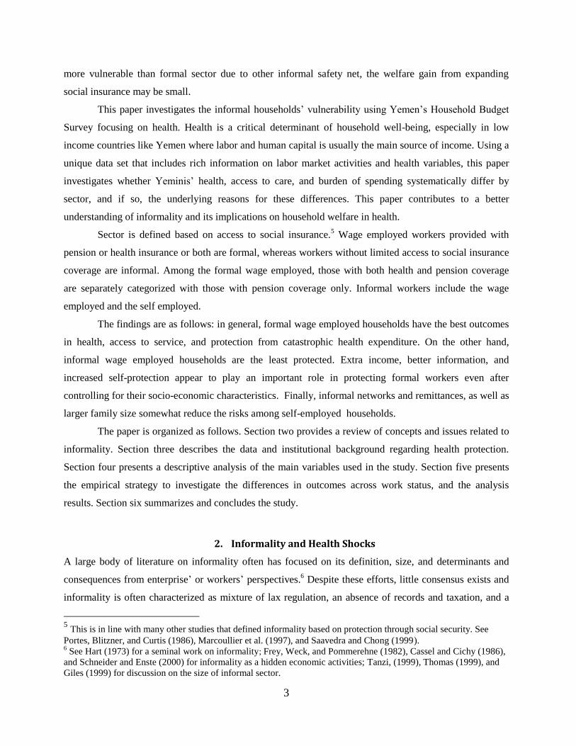
Recall that among all employed workers, those who are wage employed and provided with pension are

categorized as formal workers; other wage workers and the self-employed are categorized as informal

workers (See Figure 1). Among formal workers, a small fraction reported they received employer provided

health insurance. Households with anyone working for pension providing employers are referred to as

formal households. Among informal households, if all employed workers in the household are self-

employed, they are categorized as self-employed households.

Formal workers largely overlap with public sector workers. The proportion of public workers

among formal workers is 97%, and the proportion of formal workers among public workers is 89%. About

25% of working individuals are formal. Among formal workers, about 28% are covered by health

insurance. Informal wage employees work mostly in the private sector. They count for roughly 38% of the

employed. The rest, 37% of the employed, is self-employed (Table 1).14

The proportion of formal workers

is higher in urban areas, while the proportion of informal wage workers and self-employed workers are

higher in rural areas.

14

Throughout the paper, outcomes are presented by household or worker type: formal workers with health insurance

(formal with HI), formal workers with pension coverage only (formal with PN), informal wage workers without any

social insurance (informal wage), and self employed.

8

Figure 1. Category of workers:

by employment status and social insurance coverage

There are clear differences in demographic characteristics across different types of workers.

Several of these differences are more striking in urban than rural areas. Formal workers are significantly

more educated with more than half having received tertiary education. On the other hand, self-employed

workers are the least educated group; about half (51%) have no schooling. Educational attainment is a lot

higher in urban areas, and the urban/rural educational gap is particularly larger for informal wage workers.

Self-employed workers tend to have larger families with more children, live in rural areas, and work in

agriculture. One interesting observation here is that formal workers (especially those without health

insurance) are more likely to have multiple jobs, particularly in rural areas. The formal sector, which

overlaps with the public sector, consists of mostly male workers. Female employment is extremely low,

though urban women have slightly higher chances of work, especially in the formal sector. Informal wage

employed workers are slightly younger than formal or self-employed workers.

Job characteristics, including benefits and years of experience, are provided among wage

employed (formal and informal) but not self-employed workers. Monthly earnings are taken from a

worker’s main occupation, regardless of the number of jobs held. Formal workers with health insurance

have the highest earnings, followed by informal wage workers, and then formal wage workers without

health insurance. Among wage workers, formal workers tend to be older and more experienced in the

current job, are paid monthly, and receive employer provided benefits such as paid leave and health

insurance. Despite higher education and longer job experience, the total monthly earnings for public sector

workers are less than those of private sector workers. This may be attributed to shorter working hours for

public sector workers.

Formal Informal

Pension

only

Pension

+ Health Ins

Wage workers Self employed

No Pension

or Health Ins

9

Household Income

In addition to labor earnings from a worker’s primary occupation, households often receive a relatively

large amount of additional income, which may act as a source of informal safety net (Table 2). The amount

of extra income varies greatly across these three groups, although the proportion of workers who have

positive extra income is similar. Formal workers are more likely to have positive pension income in the

household, implying that public employment is inter-generationally correlated. Public assistance, which

supposedly targets low income households, is somewhat evenly distributed, although the receipt is more

common among informal wage workers. Private transfers from relatives and friends, and dissaving from

assets is most common among the self-employed, which suggests their dependence on informal safety nets.

The total extra income is similar for formal households and the self-employed, but significantly lower for

informal wage employed households. These patterns consistently appear when examined separately by

region.

Earnings and income are strikingly different between urban and rural workers. Although rural

households more frequently receive private transfers, the average amount is larger for urban households.

Sales and interest, and other types of income occur more frequently and in larger amounts for urban

households. When income quintiles are calculated based on household nonfood consumption, formal

households are more likely to be found in higher income quintile groups. In urban areas, informal wage

workers are found in higher income quintiles than the self-employed. Rural workers are more likely to

hold multiple jobs. Despite large urban/rural income discrepancies, public transfers are allocated similarly,

which again raises concerns about targeting of the public safety net programs.

Health Outcomes, Access, and Expenditure

Health outcomes include indicators of severe illness (disability or chronic diseases), non-chronic disease

and accident for adults, and indicators of stunting, underweight, and severe illness for children under six

(Table 3). Access to health service is measured with indicators of assisted delivery, medical help when

sick, and child immunization. Financial burden due to health spending is measured as per capita health

expenditure in the household. Finally, indicators of catastrophic expenditure are based on the proportion of

health expenditure out of nonfood consumption.

Child outcomes reconfirm the serious health situation in Yemen. A significant proportion of

children are severely stunted, and the incidence of underweight and illness is also high. Nutrition outcomes

are slightly better for children in formal sector households and the difference is clearer for urban children.

Nutrition outcomes do not necessarily go with the health outcomes: Nutrition status is better among urban

children, while health outcomes are better for rural children. The outcomes of formal households with

10

health insurance are no better or often worse than those of formal households without health insurance.

About 14% of women are disabled or chronically ill, and almost 23% are experiencing illness if accidents

and other non-chronic illness are included. Urban women are more likely to be ill than their rural

counterpart, and, in urban areas, formal households seem to have poorer health than informal households.

Health care service is best accessible by formal households, and the self-employed have similar or

slightly better access than informal wage employed workers. Access to care widely varies across region,

particularly in assisted delivery. Per capita expenditure on health, probably reflecting household income

level, is highest among formal and lowest among informal wage employed workers. However, based on

the incidence of catastrophic expenditure, formal households appear to be better protected from health

shocks compared to informal households.

5. What Determines Sector Assignment?

5.1 Multinomial logit

A worker is observed to be in one of the four mutually exclusive employment types: wage employment

with pension and health insurance (H), wage employment with pension only (P), wage employment

without pension or health insurance (N), and self employment (S). Let denote the unobserved

propensity for an individual i to hold j type of employment, which is determined by worker and market

characteristics. The individual is assigned to be in the type which gives the highest value for the

unobserved propensity. This means that

(1)

where is an actual type of employment that i was assigned.

Let be specified as a linear function of observable characteristics ( and unobservable

random errors following a standard normal distribution conditional on Then, and the

standard multinomial logit yields

(2)

with j=H, P, N, and S.

Using the informal wage employment (N) as a base category, the multinomial logit was estimated.

Worker’s characteristics including age, education, and marital status, and governorates dummy capturing

local characteristics including labor market conditions are added. Subsamples of locality of residence and

employment status are also considered.

11

Table 4 shows the results from multinomial logit estimation.15

As the informal wage employment

is the base category, the estimates read the relative propensity of working in other types of employment

rather than informal wage employment. Age, marriage, and education are positively associated with formal

employment. That is, older and better educated workers are significantly more likely to work in formal

sector than informal. The effects of some variables are heterogeneous across urban and rural areas. In

urban areas, secondary education and above is negatively related to self employment rather than informal

wage employment, and being a household head and having a pensioner in the household are significantly

related to formal sector working. Also being born at current locality of residence is negatively related to

informal wage employment, implying that those who lack local network may tend to work in informal

wage employed jobs. In rural areas, however, those with secondary and above education and social

network by being born in the same locality tend to work in self employment rather than informal wage

employment.

The coefficients of each estimation, taken together and examined with the likelihood ratio test,

shows significant differences from zero for both urban and rural areas. This means an overall non random

sector assignment. In order to examine if sector assignment even between formal with health and pension

coverage (H) and pension only (P) is statistically different across observable characteristics, the null

hypothesis that difference in the coefficients of column (1) and (2) is zero is tested. For urban areas, the

Chi Square value is 15.8 and the null hypothesis is rejected only at 10% level whereas, in rural areas, the

Chi Square value is 26.5 and the null hypothesis is rejected at 1% level. This implies that assignment

between each type of employment including H and P is also nonrandom, although workers in H and P in

urban areas are quite similar.

5.2 Selectivity Corrected Outcomes

Let the outcomes ( ) such as wage and health be determined jointly with sector assignment. Then

, where j=H, P, N, S. Taking conditional expectation over all individuals on sector

assignment yields Selectivity into each type of employment implies

that and the Ordinary Least Squares (OLS) estimate is not consistent. Following Lee

(1983) and the Handbook of Econometrics (1984), the selectivity corrected model is estimated as

15

The multinomial logit model assumes the Independence of Irrelevant Alternatives (IIA) property of each error terms ( . This

implies that each choice of employment type independently takes place. If workers are first assigned to the formal and informal

sector, and then subsequently assigned either to H or P, and N or S, this assumption no longer holds. Alternatively, if workers are

first assigned to wage and self employment and then, within wage employment, assigned between H, P, or N, the IIA assumption

is violated. HAUSMAN TEST

12

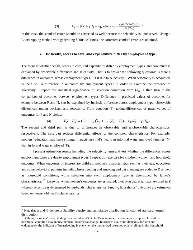
(3) , where

.16

In this case, the standard errors should be corrected as well because the selectivity is unobserved. Using a

Bootstrapping method with generating 100 times, the corrected standard errors are obtained.

6. Do health, access to care, and expenditure differ by employment type?

The focus is whether health, access to care, and expenditure differ by employment types, and how much is

explained by observable differences and selectivity. That is to answer the following questions: Is there a

difference in outcomes across employment types?; Is it due to selectivity?; When selectivity is accounted,

is there still a difference in outcomes by employment types? In order to examine the presence of

selectivity, I report the statistical significance of selection correction term ( . I then turn to the

comparison of outcomes between employment types. Difference in predicted values of outcome, for

example between P and N, can be explained by intrinsic difference across employment type, observable

differences among workers, and selectivity. From equation (3), taking differences of mean values of

outcomes for P and N yields:

(4)

.

The second and third part is due to differences in observable and unobservable characteristics,

respectively. The first part reflects differential effects of the common characteristics. For example,

mothers’ education may have stronger impacts on child’s health in informal wage employed families (N)

than in formal wage employed (P).

I present estimation results including the selectivity term and test whether the differences across

employment types are due to employment types. I repeat this exercise for children, women, and household

outcomes. When outcomes of interest are children, mother’s characteristics such as their age, education,

and some behavioral patterns including breastfeeding and smoking and qat chewing are added to Z as well

as household conditions, while selection into each employment type is determined by father’s

characteristics. 17

Likewise, when women’s outcomes are estimated, their own characteristics are used in Z

whereas selection is determined by husbands’ characteristics. Finally, households’ outcomes are estimated

based on household head’s characteristics.

16

Note that and denote probability density and cumulative distribution function of standard normal

distribution. 17

Although mothers’ breastfeeding is expected to affect child’s outcomes, the reverse is also possible: child’s

nutritional condition may induce mothers’ behavioral change. In order to avoid simultaneous decision and

endogeneity, the indicator of breastfeeding is one when the mother had breastfed other siblings in the household.

13

6.1 Children’s nutrition and health

Selectivity corrected estimation of severe stunting in urban and rural areas show several consistent patterns

(Table 6-7). Mothers’ age and education, if not monotonically, reduce the likelihood of stunting. The

number of children under six is associated with stunting, suggesting resource (food and nutrients)

constraints as main factor in child’s malnutrition. Income quintiles are not significant determinants of

stunting, whereas water supply and quality have significant effects. Having enough water supply,

especially inside a house without having to fetch, and treating water can significantly reduce stunting. The

coefficients of selectivity are statistically significant for some employment types, meaning that unobserved

characteristics associated with employment selection affect child’s nutrition.

There is heterogeneity in results across regions and employment types. In rural areas, mothers’

behavior has significant effects on child’s nutrition as expected: breastfeeding has positive effects, whereas

their smoking and qat chewing adversely affects child’s nutrition. However, in urban areas, mothers’

behavioral variables are not such significant determinants of severe stunting. The magnitude of water

treating effects on severe stunting is larger and varies more widely in rural areas than urban: variation

ranges from 10 to 30 percentage points by employment types in rural areas, but from 5 to 11 percentage

points in urban areas. In urban areas, unobservable selectivity has positive effects in self employed

households, while in rural areas it has negative effects in informal wage employment.

Similar results are found for child’s underweight, another indicator of nutrition, and child’s health

captured by the indicator of illness. The magnitude of impacts is sometimes different for health than

nutrition measures.18

The effects of water supply and quality are strongly associated with child’s health as

well as nutrition. Mother’s smoking and qat chewing is more closely related with child’s health than

nutrition. Mothers’ smoking and qat chewing increase the probability of ill health by 6 to 17 percentage

points. Meanwhile, mother’s breastfeeding is very closely with child’s nutrition, but has nonsignificant

effect on illness.

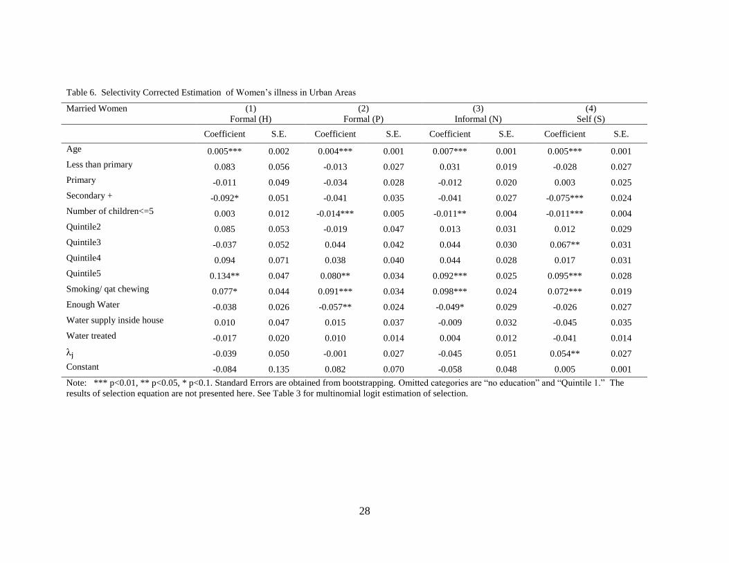
6.2 Women’s health

Women’s illness is an indicator of chronic disease, non-chronic and minor illness, and accidents, and the

estimation results are presented in Table 6 and 7. For both regions, the likelihood of illness increases with

women’s age, but decreases with education. Women’s smoking and qat chewing has strong and significant

effect on health. Water supply and quality condition is also an important determinant of women’s health as

it was for child’s health. Number of children under six is negatively associated with women’s illness.

Mothers with young children are probably more health conscious and careful not to fall ill. Alternatively,

18

The results for severe underweight and illness were not presented here, as they are similar to those of severe

stunting.

14

healthier women may have higher parity as well as low infant fatality. Selectivity is statistically significant

for some employment types.

Household income has little to do with women’s health indicator in rural areas. In urban areas,

however, the highest income quintile is strongly associated with women’s illness. This is a puzzling result

and calls for caution in interpreting. Positive relationship between income and illness can be explained if

higher income women have better access to medical service and more likely to learn about their illness.

This suggests the limitation of self reported health measures and the importance of objective measures

such as the ones based on BMI or more objective self reported measures.19

6.3 Access to Care and Health Expenditure

Among the three variables (indicators of child immunization, assisted delivery, and medical help when

sick) capturing access to health care, I present estimation results for medical help in case of illness.

Likewise, among a few measures capturing household health expenditure, I present the results for the

proportion of health expenditure among total consumption. For these estimations, I added an indicator of

presence of household member with disability. Panels A and B in Table 8 and 9, respectively, show the

results for urban and rural areas. 20

Older women and those with young children have less access to health service, especially in rural

areas, which may reflect their limited mobility to utilize health service. The effects of education are not

monotonous. In urban areas, women with higher education generally have better access, whereas those

with primary education are often worse off than their no education counterparts in rural areas.

As noted earlier, health expenditure occurs mainly to those well off households that can afford to

pay for health service and those with severe illness. The proportion of health expenditure among household

consumption decreases with education of the head and household income level. Having a household

member with disability significantly increases household health expenditure.

6.4 Health, access to care, and health expenditure across employment types

Having examined each outcome of interest with selection corrected estimation, I now turn to differences in

outcomes across employment types. Separately for urban and rural areas, I examine whether the difference

in outcomes are statistically meaningful. These differences are decomposed into three parts as specified in

equation (5). In all cases, informal wage employed (N) is used for base category.

19

The limitations of subjective self reported health measures in assessing physical capacity are widely recognized.

For review of health measures, see Currie and Madrain (1999). 20

Results that are not presented here due to the limited space can be obtained from author upon request.

15

Findings show that child’s severe stunting is significantly more prevalent among informal sector

households in both urban and rural areas. In urban areas, the all the paired differences are statistically

significant, and the likelihood of severe stunting is highest among self employed and lowest among

pension-only formal households. In rural areas, there is little difference within informal sector between

wage employed and self employed. Formal sector households are overall better off than informal ones,

despite high chances of stunting among health insured households because of better outcomes among

pension only formal households. The gap between the worst and best group is almost 7 percentage points

(3.4-(-3.5)pp) in urban and 5.5 percentage points (1.1-(-4.4)pp) in rural areas. In most cases except rural

(H-N) difference, differences due to observable characteristics have the same sign with the overall

differences, implying that the predicted outcome difference is consistent with their observable differences.

However, even counting for observable differences, there exists an outcome differential for observationally

identical households.

Women’s illness shows similar patterns in that formal households fare better than informal

counterparts, and this is clearer in rural areas. However, in rural areas, the proportion explained by

observable differences is relatively small and there is wide variation in differences due to intrinsic features

of employment and unobservable characteristics.

In terms of access to service, health insured households in urban areas significantly have better

access to medical help than other households by about 13.7 percentage points. In rural areas, the paired

differences across households are muted. I tested the differential access to service using other variables

such as assisted delivery. It also shows that formal households especially the health insured ones in urban

areas tend more to utilize medical service in child delivery.

Finally, the proportion of health spending out of household expenditure is lowest for households

with pension only and highest for health insured households. Households with health insurance especially

in rural areas have significantly higher health spending compared to their income. This suggests that health

insurance plays a role in increasing households’ access to medical service especially in urban areas, but

does little in reducing expenses.

7. Does Informal Safety Net Vary with Employment type?

7.1 Nonlabor Transfers and borrowing

Nonlabor transfers including public transfers from government and public programs, private transfer from

NGOs and religious groups and other types of income would serve as an informal safety net in the case of

external shock. As shown earlier, a disabled household member is a distress factor in health expenditure

especially for informal sector households (See Table 9). I examine to what extent extra nonlabor income

16

reduces the financial burden associated with household member with disability and how it varies with

household type.

Inter-temporal resource allocation – savings and loans– is a commonly used risk coping

mechanism. Unfortunately, information on savings is not available. However, information on loans is

available. Households often resort to informal sources such as friends and relatives (not residing together)

rather than banks or money lenders to borrow money.21

The likelihood of borrowing increases with the

presence of a disabled household member. The question is again the extent to which the health shock

increases the likelihood of borrowing, and how it varies with household types.

The coefficients of the indicator of disabled household member in the regressions on indicators of

transfer and borrowing are presented in Table 10. In urban areas, disabled household member significantly

increases the likelihood of transfer incomes among informal households by 6 percentage points. Borrowing

also increases with the residence of disabled household member by 6 to 13 percentage points. The

likelihood of borrowing in presence of disabled household member is the largest for the self employed. In

rural areas, the likelihood of receiving transfer income due to disability is highest among formal

households without health insurance. The incidence of borrowing increases with disabled household

member by 9 to 11 percentage points, and is slightly higher for informal households.

8. Conclusion

Like other developing countries and transition economies, the informal sector provides many Yemenis

work opportunities and consists of a large proportion of the labor market. A substantial proportion of the

wage employed and almost of all self employed workers, not covered by any social insurance programs,

are almost 70 percent of workers. About 52 percent of households do not have anyone working in formal

sector. These workers and their households are believed to be more vulnerable to various risks due to the

limited access to social insurance. Health risks are among the most common risks faced by many

individuals and households, and particularly so in Yemen where national health outcomes are known to lag

behind.

This paper investigated the relationship between informality and health risks, noting that there is

little empirical evidence of differential vulnerability to risks across employment types. I first outlined the

main characteristics of workers by employment and coverage status. Findings show that formal wage

workers, mostly public sector workers, tend to be substantially more educated, older, and more

experienced. They generally fall on a higher income quintile, although their earnings are no larger than

those of informal wage workers. They are less likely to work in the agriculture sector, and more likely to

21

Sources of the outstanding loan include relatives (30%), friends and neighbors (35%), and traders (29%).

17

receive regular payment and benefits. Formal wage employed households are more likely to have current

pensioners, implying a high intergenerational correlation of public sector jobs. Among informal workers,

self-employed workers are less educated than wage employed workers, but their income level is not lower,

partly due to private transfer and sales income. A large discrepancy in worker and household

characteristics was found between urban and rural areas.

Health, access to service, and health expenditure in the household widely vary along the

employment types. Selection corrected model was estimated in order to account for unobservable

heterogeneity that affects sector assignment in determining health related outcomes, as well as observed

characteristics. In most cases, unobserved heterogeneity significantly affects outcomes of interest,

implying that omitting this would bias the estimates. Outcomes are quite different across different

employment types of household heads (child’s father and women’s husband), even when considering for

all these observable differences in characteristics and locality of residence. Differences between formal

and informal households with observationally identical characteristics still persisted.

Outcomes are, in many cases, better for formal than informal households and these gaps persist

even for observationally equivalent workers. The results suggest that health insurance provides little

explanation on better outcomes among formal workers. It may even increase the households’ health

expenditure due to increased access to service, especially in rural areas. In the presence of disabled

workers, informal households face a significant increase in health spending. This is likely to be financed

by transfer income and borrowing, which serve as informal safety net.

Given a wide heterogeneity between formal and informal and even within those sectors, in their

exposure to health risks, health outcomes, coping mechanism, and spending, and also their poverty, more

research is needed to find a suitable insurance scheme that combines risk pooling and saving for the poor.

In the mean time, rather than providing protection through work, a general approach would be more

appropriate to address widespread health and malnutrition problems. For example, child stunting and

related diseases are preventable by early intervention including micronutrient fortification and education

on breastfeeding practice (Cho and Rassas, 2009). As shown in the results, water supply and quality

condition as well as mother’s behavior are very important factors in health, and should be promoted

regardless of employment status or availability of social insurance.

18

References

Adam, Markus C. and Victor Ginsburgh. 1985. "The Effects of Irregular Markets on Macro-economic

Policy: Some Estimates for Belgium," European Economic Review, 29:1, pp. 15-33.

Assaad, Ragui. 1997. “The Effects of Public Sector Hiring and Compensation Policies on the Egyptian

Labor Market,” World Bank Economic Review, 11(1), 85-115.

Baeza, Cristian and Truman Packard. 2006. Beyond Survival: Protecting Households from Health Shocks

in Latin America, World Bank. Washington DC.

Bagachwa, M. S. D. and A. Naho. 1995. "Estimating the Second Economy in Tanzania," World

Development, 23:8, pp. 1387-99.

Behrman, J. R. 1997. “Intrahousehold distribution and the family” in Handbook of population and family

economics, ed. M. R. Rosenzweig and O. Stark. Amsterdam: North-Holland Publishing Company.

Canagarajah, Sudharshan and S. V. Sethuraman. 2001. “Social Protection and the Informal Sector in

Developing Countries: Challenges and Opportunities,” Social Protection Discussion Paper Series,

0130. World Bank, Washington DC.

Carneiro, F., A., Henley, and R. Arabsheibani, 2009. “On Defining and Measuring the Informal Sector:

Evidence from Brazil,” World Development 37 (5): 992-1003.

Cassel, D. and U. Cichy, 1986. “Explaining the Growing Shadow Economy in East and West: A

Comparative Systems Approach,” Comparative Economic Studies. 28: 20-41.

Castells, M. and A. Portes, 1989. World underneath: The Origin, Dynamics, and Efforts of the Informal

Economy. In A. Portes, M. Castells, and L. Benton (Eds.), The Informal Economy Studies in

Advanced and Less Developed Countries (pp. 11-37) Baltimore: Johns Hopkins Press.

Chiappori, 1992. “Collective labor supply and welfare.” Journal of Political Economy 100 (3): 437-467.

Chiappori, 1997. “Introducing Household Production in Collective Models of Labor Supply.” Journal of

Political Economy 105(1): 191- 209.

Cho, Y. and B. Rassas. 2009. “Unfinished Agenda: Child Malnutrition in MENA” mimeo, World Bank,

Washington DC.

Cohen, B., & House, W. J. (1996). Labor Market Choices, Earnings and Informal networks in Khartoum,

Sudan. Economic Development and Cultural Change, 44(3), 589–618.

19

Cunningham, W. V., & Maloney, W. F. (2001). Heterogeneity among Mexico’s microenterprises: An

application of factor and cluster analysis. Economic Development and Cultural Change, 50(1),

131–156.

Currie, J. and B.C.Madrian, 1999, “Health, Health Insurance and the Labor Market” in O. Ashenfelter and

D. Card (eds.), Handbook of Labor Economics v. 3c, New York: Elsevier, 3309-3416.

De Soto, H., 1989. The Other Path, Harper and Row, New York.

Dilnot, A., and C., Morris. 1981. What Do We Know About the Black Economy in the United Kingdom?

Fiscal Studies, 2, 163-79.

Ehrlich, Isaac, and Gary Becker. 1972. “Market Insurance, Self Insurance, and Self Protection.” Journal of

Political Economy, Vol. 80: 623-48.

Elbadawi, Ibrahim, and Norman Loayza. 2008. “Informality, Employment, and Economic Development in

the Arab World,” The World Bank, Washington DC.

El Saharty, Sameh and Akiko Maeda, 2006. Egypt Health Sector Brief. Middle East and North Africa,

World Bank, Washington DC.

Fairbank, Alan. 2009. Health Financing Modalities in Yemen: Possibilities for Results Based Financing

and Social Health Insurance, Yemen Health Sector Review. The World Bank, Washington DC.

Feige, Edgar L. 1979. "How Big is the Irregular Economy?" Challenge, 22:1, pp. 5-13.

Frey, B., H. Weck, and W. Pommerehne, 1982. Has the Shadow Economy Grown in Germany? An

Exploratory Study. Review of World Economics, 118. 499-524.

Friedman, Eric, Simon Johnson, Daniel Kaufmann, and Pablo Zoido-Lobaton. 2000. “Dodging the

Grabbing Hand: The Determinants of Unofficial Activity in 69 Countries.” Journal of Public

Economics, 76, 459-93.

Giles, David E. A. 1999a. "Measuring the Hidden Economy: Implications for Econometric Model-ling,"

Economic Journal. 109:456, pp. 370-80.

Gindling, T. "Labor Market Segmentation and the Determination of Wages in the Public, Private-Formal,

and Informal Sectors in San Jose, Costa Rica," Economic Development and Cultural Change 39

(April 1991): 585.

Guerrero-Serdan, Gabriela. 2009. “The Effects of the War in Iraq on Nutrition and Health: An Analysis

Using Anthropometric Outcomes of Children,” MPRA Working Paper #14056.

20

Glewwe, Paul and Gillette Hall, 1998. “Are Some Groups More Vulnerable to Macroeconomic Shocks

than Others? Hypothesis Tests Based on Panel Data from Peru,” Journal of Development

Economics, 56, 181-206.

Grossman, 2000. “The Human Capital Model.” In Handbook of Health Economics, ed. A.J. Culyer and

J.P. Newhouse. Amsterdam: Elsevier

Hart, K. 1973. The Informal Income Opportunities and Urban Employment in Ghana. Journal of Modern

African Studies. 11. 61-89.

Heckman, J., & Sedlacek, G. 1985. Heterogeneity, aggregation and market wage functions: An empirical

model of self-selection in the labor market. Journal of Political Economy, 93, 1077–1125.

Maloney, William. 2004. “Informality Revisited,” World Development, 32 (7), 1159-78.

Marcoullier, D., Ruiz de Casilla, V., & Woodruff, C. 1997. Formal measures of the informal-sector wage

gap in Mexico, El Salvador, and Peru. Economic Development and Cultural Change, 45(2), 367–

392.

Lee, L. "Generalized Econometric Models with Selectivity," Econometrica 51 (March 1983): 507-12.

Lundberg, Shelly J., Robert A. Pollak, and Terence J. Wales. 1997. "Do Husbands and Wives Pool Their

Resources? Evidence from the United Kingdom Child Benefit" Journal of Human Resources 32

(3): 463-480.

Perry, Guillermo, Omar Arias, Pablo Fajnzylber, William Maloney, Andrew Mason, and Jaime Saavedra,

2007. Informality: Exit and Exclusion, The World Bank, Washington DC.

Portes, A., Blitzner, S., & Curtis, J. (1986). The urban informal sector in Uruguay: Its internal structure,

characteristics, and effects. World Development, 14(6), 727–741.

Pradhan, M., and A. van Soest 1995. Formal and informal sector employment in urban areas of Bolivia.

Labour Economics, 2, 275–297.

Pradhan, M., & van Soest, A. (1997). Household labor supply in urban areas of Bolivia. Review of

Economics and Statistics, 79(2), 300–310.

Pyle, D. 1989. Tax Evasion and the Black Economy. New York, NY: St. Martin’s Press.

Saavedra, J., & Chong, A. (1999). Structural reform, institutions and earnings: Evidence from the formal

and informal sectors in urban Peru. Journal of Development Studies, 35(4), :95–116.

Schneider, Fredrich and Dominik Enste, 2000. “Shadow Economies: Size, Causes, and Consequences,”

Journal of Economic Literature, Vol. 38, 77-114.

Tanzi, Vito. 1999. "Uses and Abuses of Estimates of the Underground Economy, Economic Journal.

109:456 pp. 338-40

21

Thomas, James. 1999. "Quantifying the Black Economy: 'Measurement without Theory' Yet Again?"

Economic Journal, 109:456, pp. 381-89.

Unite Nations and World Bank, 2003. Joint Iraq Needs Assessment: Health.

Wiles, P. 1987. The Second Economy, Its Definitional Problems. In: S. Allesandrini and B. Dallago,

Editors, The Unofficial Economy: Consequences and perspectives in different economic systems,

Gower Publishing Company. UK.

World Bank. 2005. Social Protection in Transition: Labor Policy, Safety Nets and Pensions. A Policy

Note. Middle East and North Africa, Washington DC.

World Bank. 2009. Public Health Expenditure Review for the Period from 2004 to 2007. World Bank.

Washington DC.

22

Table 1. Worker Characteristics by Employment Status, Coverage of Social Insurance, and Region

All Urban Rural

Formal Informal Formal Informal Formal Informal

(H) (P) (N) (S)

(H) (P) (N) (S)

(H) (P) (N) (S)

A. Worker Characteristics

Proportion 7.2% 18.0% 37.6% 37.3%

9.3% 22.6% 36.9% 31.2%

3.9% 11.2% 40.2% 44.7%

Urban 56.4% 47.2% 29.9% 20.9%

100.0% 100.0% 100.0% 100.0%

0.0% 0.0% 0.0% 0.0%

Age 35.7 34.6 31.7 37.8

37.5 36.5 31.0 35.8

33.4 33.0 31.9 38.3

Male 91.1% 90.2% 95.9% 94.4%

86.1% 81.7% 89.6% 95.2%

97.6% 97.8% 98.6% 94.2%

No schooling 10.9% 8.4% 35.0% 50.6%

9.5% 8.0% 20.2% 33.7%

12.7% 8.7% 41.0% 55.2%

Primary and below

7.9% 7.2% 25.1% 17.6%

5.5% 7.0% 22.6% 22.2%

11.0% 7.3% 26.2% 16.3%

Secondary 25.3% 25.1% 21.9% 17.6%

21.4% 20.3% 25.6% 24.9%

30.4% 29.4% 20.4% 15.7%

Tertiary and above

55.9% 59.4% 18.0% 14.2%

63.6% 64.8% 31.5% 19.2%

45.9% 54.6% 12.4% 12.8%

Household Size

8.2 8.6 8.6 9.7

7.8 8.2 8.2 9.8

8.7 8.9 8.8 9.6

Num. of Children

1.5 1.6 3.4 4.0

1.3 1.5 2.8 3.7

1.8 2.0 3.6 4.1

Agriculture 1.0% 1.6% 27.6% 59.3%

1.1% 1.1% 7.7% 13.6%

0.9% 2.0% 36.4% 71.4%

Num, jobs >1 17.8% 29.7% 25.4% 12.7%

14.0% 19.3% 10.0% 6.3%

22.5% 38.5% 32.4% 14.4%

B. Job Characteristics

Monthly earnings (YR)

35,699 25,876 31,512 .

41,256 28,513 36,283 .

28,521 23,523 29,490 .

Hours per week

42.5 39.4 49.0 .

41.6 38.3 50.8 .

43.7 40.4 48.2 .

Paild Leave 97.6% 97.8% 5.7% .

96.7% 96.0% 12.6% .

98.8% 99.4% 2.8% .

Health Insurance

100.0% 0.0% 1.7%

100.0% 0.0% 4.2%

100.0% 0.0% 0.6%

Public sector 93.9% 98.7% 5.2% .

92.1% 97.7% 10.6% .

96.3% 99.5% 2.9% .

Num. years of this job

11.1 10.4 6.3 . 12.3 11.6 5.3 . 9.5 9.4 6.7 .

23

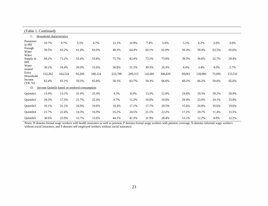
(Table 1. Continued)

C. Household characteristics

Pensioner

in HH 10.7% 9.7% 5.5% 4.7%

12.1% 10.9% 7.4% 5.6%

5.1% 6.2% 2.6% 3.6%

Enough

Water 50.5% 63.2% 61.4% 63.0%

48.3% 64.4% 60.1% 61.0%

56.3% 59.4% 63.5% 65.6%

Water

Supply in

HH

68.2% 71.2% 53.4% 53.8%

75.7% 82.4% 73.2% 73.9%

39.3% 36.6% 22.7% 29.4%

Water

treated 30.1% 24.4% 20.0% 15.6%

36.8% 31.2% 30.3% 26.3%

4.4% 3.4% 4.0% 2.7%

Extra

Household

Income

(YR, %)

152,262 164,524 92,269 168,124

223,798 209,313 142,681 306,829

69,061 128,900 75,095 133,531

62.4% 65.1% 59.5% 65.8%

58.1% 63.7% 59.3% 66.6%

68.2% 66.2% 59.6% 65.6%

D. Income Quintile based on nonfood consumption

Quintile1 13.4% 13.1% 31.4% 25.4%

4.5% 6.0% 13.3% 12.0%

24.8% 19.3% 39.2% 28.9%

Quintile2 18.3% 17.5% 21.7% 22.4%

9.7% 11.2% 16.0% 16.9%

29.4% 23.0% 24.1% 23.8%

Quintile3 16.1% 21.1% 16.9% 19.8%

16.4% 17.1% 17.7% 20.5%

15.6% 24.8% 16.6% 19.6%

Quintile4 21.7% 22.4% 14.3% 16.9%

25.2% 24.5% 21.1% 22.2%

17.2% 20.7% 11.4% 15.5%

Quintile5 30.6% 25.9% 15.7% 15.6%

44.1% 41.2% 31.9% 28.4%

13.1% 12.2% 8.8% 12.2%

Notes: H denotes formal wage workers with health insurance as well as pension, P denotes formal wage workers with pension coverage, N denotes informal wage workers

without social insurance, and S denotes self employed workers without social insurance.

24

Table 2. Health, Access to Care, Expenditure by Household Type

All Urban Rural

Formal Informal Formal Informal Formal Informal

(H) (P) (N) (S)

(H) (P) (N) (S)

(H) (P) (N) (S)

Health

Wo

men

Chronic

disease 8.0% 6.9% 8.2% 10.0%

9.3% 8.3% 8.9% 11.1%

2.8% 2.9% 7.4% 8.7%

Illness 19.8% 17.1% 18.8% 19.3%

21.4% 19.3% 20.9% 21.6%

13.2% 10.8% 16.0% 16.5%

Ch

ild

ren

Severe

Stunting 30.1% 31.0% 35.5% 36.4%

21.4% 19.9% 24.8% 27.4%

38.0% 36.6% 38.4% 38.5%

Severe

Under-weight 13.7% 9.8% 13.8% 15.0%

9.1% 8.4% 10.5% 13.6%

17.9% 10.5% 14.7% 15.3%

Illness 19.5% 19.8% 19.5% 17.8%

22.9% 22.9% 22.6% 22.9%

16.4% 18.2% 18.6% 16.7%

Access to Service

Wo

men

Assisted

Delivery 42.3% 40.1% 30.0% 29.6%

61.4% 58.9% 52.4% 52.1%

20.1% 27.7% 22.5% 24.1%

Medical Help

when ill 92.2% 87.3% 85.0% 85.8%

95.3% 89.9% 89.4% 89.8%

88.1% 85.3% 83.5% 84.8%

Ch

ild

ren

Immunization 54.0% 51.8% 41.0% 41.3%

60.1% 60.7% 55.5% 56.5%

48.6% 47.2% 36.9% 38.0%

Expenditure

Ho

use

hold

Log(per

capita

spending)

8.3 8.0 8.0 8.1

8.6 8.3 8.4 8.2

7.7 7.9 7.8 8.0

Catastropic 1 8.8% 10.3% 12.4% 12.1%

10.1% 8.5% 10.0% 9.4%

7.2% 11.6% 13.3% 12.8%

Catastropic 2 4.9% 5.6% 7.2% 7.3%

5.5% 4.5% 5.8% 4.3%

4.2% 6.4% 7.7% 8.0%

Notes: Severe stunting and underweight is defined as 1 when the standardized z-score based on Body Mass Index for each measure is below -3 Standard Deviation, and 0 otherwise.

25

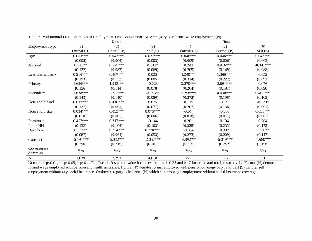
Table 3. Multinomial Logit Estimates of Employment Type Assignment: Base category is informal wage employment (N)

Urban Rural

Employment type (1)

Formal (H)

(2)

Formal (P)

(3)

Self (S)

(4)

Formal (H)

(5)

Formal (P)

(6)

Self (S)

Age 0.053*** 0.047*** 0.027*** 0.046*** 0.048*** 0.046***

(0.005) (0.004) (0.003) (0.009) (0.006) (0.003)

Married 0.311** 0.525*** 0.131* 0.242 0.916*** -0.341***

(0.122) (0.087) (0.069) (0.205) (0.149) (0.088)

Less than primary 0.916*** 0.887*** 0.025 1.240*** 1.366*** 0.052

(0.193) (0.132) (0.085) (0.314) (0.222) (0.091)

Primary 1.636*** 1.513*** -0.023 2.270*** 2.601*** 0.076

(0.156) (0.114) (0.078) (0.264) (0.191) (0.090)

Secondary + 2.638*** 2.722*** -0.186** 3.298*** 4.030*** 0.405***

(0.148) (0.110) (0.080) (0.272) (0.196) (0.103)

Household head 0.637*** 0.416*** 0.075 0.115 -0.040 -0.170*

(0.127) (0.091) (0.077) (0.207) (0.138) (0.091)

Household size 0.034*** 0.033*** 0.075*** -0.014 -0.003 0.036***

(0.010) (0.007) (0.006) (0.018) (0.011) (0.007)

Pensioner 0.457*** 0.317*** -0.144 0.261 0.194 0.264

in the HH (0.132) (0.104) (0.103) (0.328) (0.233) (0.172)

Born here 0.223** 0.234*** 0.270*** -0.334 0.332 0.250**

(0.087) (0.064) (0.053) (0.273) (0.209) (0.117)

Constant -6.194*** -5.032*** -2.052*** -4.892*** -6.019*** -1.680***

(0.296) (0.215) (0.161) (0.525) (0.392) (0.196)

Governorate

dummies Yes Yes Yes Yes Yes Yes

N 1,039 2,391 4,018 272 775 3,313

Note: *** p<0.01, ** p<0.05, * p<0.1. The Pseudo R squared value for the estimation is 0.25 and 0.17 for urban and rural, respectively. Formal (H) denotes

formal wage employed with pension and health insurance, Formal (P) denotes formal employed with pension coverage only, and Self (S) denotes self

employment without any social insurance. Omitted category is Informal (N) which denotes wage employment without social insurance coverage.

26

Table 4. Selectivity Corrected Estimation of Child’s Severe Stunting in Urban Areas

Children <6 (1)

Formal (H)

(2)

Formal (P)

(3)

Informal (N)

(4)

Self (S)

Coefficient S.E. Coefficient S.E. Coefficient S.E. Coefficient S.E.

Child’s age 0.037*** 0.007 0.014* 0.009 0.013 0.008 0.027*** 0.007

Age -0.003 0.002 -0.007*** 0.002 -0.001 0.001 -0.005** 0.002

Less than primary -0.078** 0.037 -0.119*** 0.028 -0.019 0.020 -0.048 0.031

Primary -0.122*** 0.041 -0.096*** 0.031 -0.041 0.033 -0.040 0.035

Secondary + -0.103** 0.054 -0.077*** 0.035 -0.120*** 0.026 -0.035 0.066

Number of children<=5 0.030** 0.014 0.012* 0.007 0.015** 0.006 0.003 0.007

Quintile2 0.050 0.086 0.017 0.060 -0.049 0.028 -0.079* 0.044

Quintile3 0.075 0.082 0.059 0.047 -0.015 0.029 -0.082* 0.043

Quintile4 0.065 0.072 0.033 0.031 -0.100** 0.039 -0.086*** 0.030

Quintile5 0.107 0.077 -0.003 0.040 -0.108*** 0.031 -0.095*** 0.035

Smoking/ qat chewing -0.007 0.065 0.031 0.024 -0.025 0.028 -0.051*** 0.020

Breastfeeding -0.211 0.170 0.006 0.078 0.082 0.091 -0.018 0.087

Enough Water -0.075 0.053 -0.039 0.021 0.001 0.024 -0.019 0.012

Water supply inside house 0.018 0.023 -0.044** 0.022 -0.059*** 0.015 -0.013 0.021

Water treated -0.118*** 0.037 -0.087*** 0.014 -0.068*** 0.021 -0.029 0.018

-0.027 0.031 -0.002 0.020 0.042 0.040 0.168*** 0.041

Constant 0.218 0.152 0.485*** 0.076 0.420*** 0.082 0.669*** 0.104

Note: *** p<0.01, ** p<0.05, * p<0.1. Standard Errors are obtained from bootstrapping. Omitted categories are “no education” and “Quintile 1.” The results

of selection equation are not presented here. See Table 3 for multinomial logit estimation of selection.

27

Table 5. Selectivity Corrected Estimation of Child’s Severe Stunting in Rural Areas

Children <6 (1)

Formal (H)

(2)

Formal (P)

(3)

Informal (N)

(4)

Self (S)

Coefficient S.E. Coefficient S.E. Coefficient S.E. Coefficient S.E.

Child’s age 0.029 0.027 0.013 0.013 0.013 0.008 0.023*** 0.010

Age -0.010* 0.005 -0.008** 0.004 -0.000 0.002 -0.002 0.002

Less than primary 0.012 0.128 -0.115** 0.055 0.011 0.046 -0.069* 0.043

Primary -0.222** 0.108 -0.027 0.063 -0.085 0.057 -0.098 0.064

Secondary + 0.212 0.213 -0.167** 0.084 -0.013 0.150 -0.019 0.102

Number of children<=5 0.046 0.031 -0.005 0.011 0.001 0.009 0.011 0.007

Quintile2 -0.012 0.115 0.012 0.049 -0.062** 0.027 0.038 0.030

Quintile3 -0.090 0.112 -0.002 0.056 -0.050 0.037 0.007 0.033

Quintile4 0.143 0.140 -0.052 0.056 -0.037 0.043 0.036 0.038

Quintile5 -0.046 0.156 -0.052 0.075 -0.034 0.050 -0.015 0.047

Smoking/ qat chewing 0.255** 0.105 0.073 0.051 0.083*** 0.027 0.048* 0.029

Breastfeeding 0.010 0.330 -0.324*** 0.072 -0.090 0.083 -0.251*** 0.082

Enough Water -0.131* 0.079 0.008 0.043 -0.010 0.027 -0.055** 0.026

Water supply inside house 0.015 0.102 -0.078** 0.034 -0.023 0.032 -0.017 0.026

Water treated 0.112 0.223 -0.194** 0.090 -0.095* 0.056 -0.295*** 0.071

0.104 0.103 0.062 0.049 -0.138*** 0.028 -0.046 0.050

Constant 0.689** 0.301 0.706*** 0.156 0.252*** 0.063 0.364*** 0.088

Note: *** p<0.01, ** p<0.05, * p<0.1. Standard Errors are obtained from bootstrapping. Omitted categories are “no education” and “Quintile 1.” The

results of selection equation are not presented here. See Table 3 for multinomial logit estimation of selection.

28

Table 6. Selectivity Corrected Estimation of Women’s illness in Urban Areas

Married Women (1)

Formal (H)

(2)

Formal (P)

(3)

Informal (N)

(4)

Self (S)

Coefficient S.E. Coefficient S.E. Coefficient S.E. Coefficient S.E.

Age 0.005*** 0.002 0.004*** 0.001 0.007*** 0.001 0.005*** 0.001

Less than primary 0.083 0.056 -0.013 0.027 0.031 0.019 -0.028 0.027

Primary -0.011 0.049 -0.034 0.028 -0.012 0.020 0.003 0.025

Secondary + -0.092* 0.051 -0.041 0.035 -0.041 0.027 -0.075*** 0.024

Number of children<=5 0.003 0.012 -0.014*** 0.005 -0.011** 0.004 -0.011*** 0.004

Quintile2 0.085 0.053 -0.019 0.047 0.013 0.031 0.012 0.029

Quintile3 -0.037 0.052 0.044 0.042 0.044 0.030 0.067** 0.031

Quintile4 0.094 0.071 0.038 0.040 0.044 0.028 0.017 0.031

Quintile5 0.134** 0.047 0.080** 0.034 0.092*** 0.025 0.095*** 0.028

Smoking/ qat chewing 0.077* 0.044 0.091*** 0.034 0.098*** 0.024 0.072*** 0.019

Enough Water -0.038 0.026 -0.057** 0.024 -0.049* 0.029 -0.026 0.027

Water supply inside house 0.010 0.047 0.015 0.037 -0.009 0.032 -0.045 0.035

Water treated -0.017 0.020 0.010 0.014 0.004 0.012 -0.041 0.014

-0.039 0.050 -0.001 0.027 -0.045 0.051 0.054** 0.027

Constant -0.084 0.135 0.082 0.070 -0.058 0.048 0.005 0.001

Note: *** p<0.01, ** p<0.05, * p<0.1. Standard Errors are obtained from bootstrapping. Omitted categories are “no education” and “Quintile 1.” The

results of selection equation are not presented here. See Table 3 for multinomial logit estimation of selection.

29

Table 7. Selectivity Corrected Estimation of Women’s illness in Rural Areas

Married Women (1)

Formal (H)

(2)

Formal (P)

(3)

Informal (N)

(4)

Self (S)

Coefficient S.E. Coefficient S.E. Coefficient S.E. Coefficient S.E.

Age 0.005 0.004 -0.002 0.002 0.005*** 0.001 0.004*** 0.001

Less than primary -0.043 0.063 -0.019 0.049 0.000 0.027 0.032 0.034

Primary 0.042 0.115 -0.092*** 0.032 -0.003 0.047 -0.044 0.038

Secondary + -0.063 0.092 -0.060 0.053 -0.029 0.090 0.023 0.077

Number of children<=5 0.012 0.020 -0.019*** 0.007 -0.008 0.007 -0.004 0.005

Quintile2 0.007 0.074 -0.022 0.038 -0.020 0.019 -0.003 0.021

Quintile3 0.038 0.091 -0.010 0.032 0.007 0.025 0.003 0.021

Quintile4 0.027 0.079 0.022 0.048 0.007 0.025 0.028 0.024

Quintile5 -0.047 0.105 0.072 0.048 0.049 0.033 0.038 0.023

Smoking/ qat chewing 0.201 0.127 0.078 0.048 0.089*** 0.024 0.054* 0.030

Enough Water -0.034 0.060 0.007 0.032 0.038** 0.015 -0.019 0.026

Water supply inside house -0.057 0.082 -0.050** 0.021 -0.073*** 0.021 -0.044** 0.019

Water treated -0.023 0.117 -0.005 0.060 -0.002 0.043 -0.036 0.049

0.173* 0.092 -0.030 0.024 -0.100** 0.044 0.025 0.034

Constant 0.284 0.234 0.198** 0.080 -0.083* 0.043 0.036 0.062

Note: *** p<0.01, ** p<0.05, * p<0.1. Standard Errors are obtained from bootstrapping. Omitted categories are “no education” and “Quintile 1.” The results

of selection equation are not presented here. See Table 3 for multinomial logit estimation of selection.

30

Table 8. Selectivity Corrected Estimation of Access to Health Service

(1)

Formal (H)

(2)

Formal (P)

(3)

Informal (N)

(4)

Self (S)

A. Urban Coefficient S.E. Coefficient S.E. Coefficient S.E. Coefficient S.E.

Age 0.002 0.002 -0.001 0.001 0.001 0.001 0.000 0.000

Less than primary 0.047 0.029 -0.017 0.034 -0.010 0.028 0.012 0.018

Primary 0.025 0.020 0.073*** 0.024 0.076*** 0.018 0.080*** 0.026

Secondary + 0.047 0.038 0.051*** 0.019 0.063*** 0.019 0.046 0.034

Number of children<=5 0.002 0.008 -0.025*** 0.005 -0.016*** 0.005 -0.013*** 0.003

Quintile2 -0.005 0.034 0.002 0.043 -0.002 0.035 -0.024 0.029

Quintile3 0.003 0.032 0.040 0.056 0.005 0.033 -0.011 0.028

Quintile4 -0.025 0.044 0.081* 0.047 0.017 0.033 -0.030 0.027

Quintile5 -0.014 0.033 0.092** 0.044 0.061** 0.028 -0.021 0.027

Disabled member in the HH 0.025 0.022 0.052*** 0.014 0.040* 0.021 0.030** 0.012

-0.000 0.044 -0.078*** 0.021 0.022 0.044 -0.013 0.037

Constant 0.895 0.086 0.747*** 0.087 0.825*** 0.061 0.849*** 0.038

B. Rural Coefficient S.E. Coefficient S.E. Coefficient S.E. Coefficient S.E.

Age 0.009 0.006 -0.006*** 0.002 -0.002** 0.001 -0.004*** 0.001

Less than primary -0.199** 0.086 -0.198*** 0.059 -0.038 0.033 0.004 0.047

Primary 0.090 0.089 0.051 0.041 0.072 0.048 0.110** 0.054

Secondary + 0.175** 0.088 -0.030 0.056 0.043 0.076 -0.227 0.181

Number of children<=5 -0.020 0.026 -0.019* 0.011 -0.022*** 0.006 -0.019*** 0.006

Quintile2 0.035 0.126 0.090* 0.049 0.025 0.020 0.091*** 0.025

Quintile3 -0.047 0.130 0.111** 0.043 0.024 0.031 0.093** 0.036

Quintile4 0.298** 0.127 0.097** 0.043 -0.006 0.032 0.085*** 0.032

Quintile5 0.087 0.154 0.179*** 0.041 0.024 0.031 0.082** 0.036

Disabled member in the HH 0.117 0.110 0.037 0.036 0.018 0.022 0.048** 0.024

0.456*** 0.123 -0.047 0.041 -0.098*** 0.044 0.204*** 0.054

Constant 1.283*** 0.340 0.928*** 0.092 0.808 0.051 1.081*** 0.092

Note: *** p<0.01, ** p<0.05, * p<0.1. Standard Errors are obtained from bootstrapping. Omitted categories are “no education” and “Quintile 1.” The results

of selection equation are not presented here.

31

Table 9. Selectivity Corrected Estimation of Log (Proportion of Health Expenditure)

(1)

Formal (H)

(2)

Formal (P)

(3)

Informal (N)

(4)

Self (S)

A. Urban Coefficient S.E. Coefficient S.E. Coefficient S.E. Coefficient S.E.

Age 0.045 0.095 0.044 0.042 -0.000 0.020 0.013 0.018

Age Squared -0.001 0.001 -0.000 0.001 -0.000 0.000 -0.000 0.000

Less than primary -0.399 0.771 -0.266 0.642 -0.220 0.152 -0.057 0.184

Primary -0.564 0.539 0.483 0.590 -0.350** 0.143 -0.204 0.158

Secondary + -1.028** 0.492 0.391 0.671 -0.433** 0.196 -0.326 0.214

Smoking/ qat chewing -0.205 0.227 -0.401** 0.171 0.148 0.101 0.134 0.132

Quintile2 -0.298 0.535 -0.119 0.495 -0.169 0.145 -0.425** 0.171

Quintile3 -0.116 0.432 -0.049 0.485 -0.348** 0.136 -0.541*** 0.161

Quintile4 -0.160 0.426 0.124 0.496 -0.277** 0.121 -0.493*** 0.152

Quintile5 -0.586 0.403 -0.058 0.515 -0.412*** 0.140 -0.669*** 0.176

Disabled member in the HH 0.098 0.188 0.296* 0.176 0.311*** 0.094 0.247*** 0.093

1.250** 0.610 -0.521 0.462 0.004 0.263 -0.030 0.171

Constant -0.010 1.997 -4.424*** 1.430 -1.810*** 0.407 -2.290*** 0.366

B. Rural Coefficient S.E. Coefficient S.E. Coefficient S.E. Coefficient S.E.

Age -0.013 0.191 -0.099 0.074 -0.011 0.021 0.004 0.013

Age Squared 0.001 0.003 0.001 0.001 -0.000 0.000 -0.000 0.000

Less than primary 1.368 0.805 -0.520 0.523 -0.193 0.125 -0.023 0.149

Primary 0.895 0.864 -0.372 0.613 -0.289** 0.143 -0.067 0.178

Secondary + 1.145 0.975 -0.172 0.764 -0.418** 0.223 -0.286 0.174

Smoking/ qat chewing -0.121 0.856 0.185 0.287 -0.276*** 0.099 -0.060 0.123

Quintile2 0.038 0.615 -0.313 0.432 -0.353*** 0.110 -0.348*** 0.121

Quintile3 0.153 0.630 -0.524 0.405 -0.544*** 0.122 -0.391*** 0.126

Quintile4 -1.302 0.681 -0.003 0.462 -0.423*** 0.142 -0.301** 0.139

Quintile5 -0.846 0.722 -0.280 0.484 -0.504*** 0.158 -0.638*** 0.219

Disabled member in the HH 0.771 0.656 0.227 0.227 0.149* 0.089 0.311*** 0.098

0.469 0.934 -0.283 0.452 -0.238 0.220 -0.290 0.257

Constant -2.985 4.204 -0.561 1.915 -1.301*** 0.387 -2.392*** 0.316

Note: *** p<0.01, ** p<0.05, * p<0.1. Standard Errors are obtained from bootstrapping. Omitted categories are “no education” and “Quintile 1.” The results of

selection equation are not presented here.

32

Table 10. Decomposition of differences in outcomes

Urban Areas Rural Areas

(1)

(2)

(3)

(4)

(5)

(6)

(7)

(8)

Child: Severe Stunting

H-N -0.022*** -0.060 -0.043 0.081 0.011* 0.337 -0.029 -0.296

P-N -0.035*** -0.048 -0.032 0.045 -0.044*** 0.164 -0.021 -0.187

S-N 0.034*** 0.153 0.009 -0.128 -0.002 0.078 -0.003 -0.077

Women: Illness

H-N 0.003 -0.034 0.027 0.010 -0.034*** 0.394 -0.034 -0.394

P-N -0.014*** 0.020 0.011 -0.046 -0.051*** 0.032 -0.032 -0.051

S-N 0.006** 0.076 0.028 -0.098 0.006** 0.086 0.026 -0.106

Access: Medical help when sick

H-N 0.137*** 0.089 0.025 0.023 -0.019 0.869 0.006 -0.894

P-N 0.000 -0.123 0.016 0.107 0.025 0.054 0.001 -0.029

S-N 0.004 -0.025 -0.007 0.035 0.007 0.264 -0.014 -0.244

Expenditure: Proportion of health expenditure

H-N 0.005 1.622 -0.211 -1.406 0.255*** -1.939 -0.216 2.410

P-N -0.169*** -0.345 -0.189 0.365 -0.053** -0.312 -0.298 0.556

S-N -0.037*** 0.502 -0.040 -0.499 -0.015 0.461 -0.203 -0.273

Note: ***, **, and * in columns (1) and (5) denote statistical significance at 1%, 5%, and 10% level, respectively, from the test of the null hypothesis

33

Table 11. Informal Safety Net: The Impacts of Disabled Household Member

Dependent variables (1)

Formal (H)

(2)

Formal(P)

(3)

Informal (N)

(4)

Self (S)

A. Urban Coefficient S.E. Coefficient S.E. Coefficient S.E. Coefficient S.E.

Transfer income 0.037 0.065 0.031 0.033 0.060** 0.032 0.040** 0.020

Borrowing 0.067*** 0.023 0.093*** 0.033 0.064** 0.032 0.128*** 0.039

B. Rural Coefficient S.E. Coefficient S.E. Coefficient S.E. Coefficient S.E.

Transfer income -0.085 0.104 0.227*** 0.031 0.059*** 0.021 0.060** 0.026

Borrowing 0.018 0.085 0.092*** 0.030 0.116*** 0.045 0.113*** 0.029

Notes: The coefficients of an indicator of disabled household member are obtained from two separate regressions on transfer income and borrowing separately

for each region.