INFLUENCE OF TIDAL FORCES (THE EARTH – MOON- SUN SYSTEM) ON SOME GEOLOGICAL ...geo.phys.spbu.ru/materials_of_a_conference_2008/NLM/... · 2008-11-18 · INFLUENCE OF TIDAL FORCES

INFLUENCE OF TIDAL FORCES (THE EARTH – MOON- SUN SYSTEM)

ON SOME GEOLOGICAL PROCESSES IN THE EARTH’S CRUST

Yu.N. Avsjuk, Yu.S. Genshaft, A.Ja. Saltykovsky, Yu.F. Sokolova, and S.P. Svetlosanova

Institute of the Physics of the Earth, Russian Academy of Sciences, Moscow, 123995,

e-mail: [email protected]

Abstract. It was shown that oscillating regime of tidal evolution in the Earth – Moon – Sun system results in periodical changes of velocity rotation and incline angle of the axis rotation. According to geological data it has been distinguished epoch intervals of maximum Phanerozoic sedimentation, magmatism and folding stages. These are compared with calculated changes of velocities and orientation of the Earth rotation axis (the model of cyclic motion of tidal evolution in the Earth – Moon – Sun system.) It has shown a steady trend of high Earth’s activation during Phanerozoic epoch within the range of latitudes (20º-40º Northern latitudes) that confirms the opinion on inherent of tectonic processes. It has been established the minimal transgression for subequatorial areas and noticeable increase to the Polar latitudes, in particular for the South hemisphere. This fact is accord to the conclusion on variations of the World Ocean level in equatorial and high latitude areas at the Earth’s axial rotation of velocity change. It was demonstrated that the tidal forces in the Earth – Moon – Sun system may influence greatly on the intensity and latitudinal zoning of geological processes in the Earth’s crust.

It was shown [Avsjuk, 1996; Avsjuk et.al., 1996, 2005, 2007] that oscillating regime in the tidal evolution of

the Earth – Moon – Sun system should produce periodical changes of velocity rotation and incline angle of

the axis rotation. The increase of the Earth angle rotation velocity (+ω) should be accompanied with increase

of the World ocean level within the range of low latitudes (equatorial) and decrease ones in high latitudes

(Polar areas). Another situation has to observed with decrease of the velocity rotation of the Earth (-ω).

(Fig.1). According to the principles the latitudinal zoning has to take place in distribution (in geological scale

of time) of some geodynamical processes within the lithosphere (we mean Phanerozoic epoch only).

It was calculated the sedimentation areas (the areas of transgression and regression) in geological

intervals including of Mesozoic and Cenozoic epochs based on the Atlas of Lithological-Paleogeographical

formations (Ed. V. Khain, 1982). The latitudinal zoning of sedimentary basins in latitudinal intervals 0-20,

20-40, 40-60 to the South and to the North correlates with the periodical movement of axis rotation into the

Earth’s body and change of the rotation velocity. The intensity of sedimentary areas expansion is minimal in

Jurassic and Cretaceous and much more in Triassic and Cenozoic especially. The transgression maximum

was in latitude interval 20-40O for the North hemisphere for the all studied geological epochs. It has been

established the minimal transgression for subequatorial areas and notable increase to the more higher

latitudes, in particular for the South hemisphere.

Proceedings of the 7th International Conference "Problems of Geocosmos" (St. Petersburg, Russia, 26-30 May 2008)

336

This fact is accorded to the conclusion on variations of theWorld Ocean level in equatorial and high

latitude areas at the Earth’s axial rotation of velocity change. It has been distinguished intervals of magmatic

activation in Phanerozoic stage according geological data. These are compared with precalculated of changes

of velocity and the axis of rotation of the Earth.

The oscillating evolution of the tidal forces in the Sun-Earth-Moon system should be produce

temporal cycles in the Earth’s geodynamic processes and latitudinal shifts in the geological scale of time.

The Phanerozoic history of the Earth includes phenomena of acceleration of tectonic movements that are

marked in rock sequences of the Earth’s crust by folding, angular unconformities, fault tectonics,

emplacement of large and small intrusions, rock deformations, transgression –regression phases and so on.

Irregularity in the Earth’s tectonic history is characterized by a cycle pattern. In addition, periods of

tectonic activation and intervals between tectonic cycles have different durations. An overview of cyclic

manifestations in the Earth’s tectonic history given in V.Khain [2000]. It is devoted to analysis of quasi-

periodic tectonic activity (known as Wilson, Bertrand, and Stille cycles) with a significantly different

duration. H.Stille considered the relatively short-term (about 30 Ma) planetary orogenic phases and devided

them into epochs of relative tectonic repose. M.Bertrand devided the Earth’s geological history into five

cycles with a longer duration (Baikalian, Caledonian, Hercynian, Cimmerian, and finally, Alpine). Wilson’s

cycles are long-term ones. The cyclicity is attributed to diverse processes ranging from predominant vertical

movements, with produce geosynclinal-orogenic structures, to tectonics of lithospheric plates (convection in


337

the mantle and horizontal displacements of continents) and galactic processes (intersections of asteroids and

comets by the solar system and the Earth).

Our previous works devoted to the latitudinal shift of domains of continental sedimentation amd

magmatism in the Phanerozoic history of the Earth revealed significant correlations with the trend of tidal

evolution of the Earth – Moon – Sun system [Avsjuk et al., 2005, 2007]. Continuing these investigations, we

analyzed the areas (within the present day continents) of the Caledonian (terminal Early – initial Middle

Paleozoic), Hercynian (terminal Devonian – initial Triassic), Cimmerian (Mesozoic), and Alpine (terminal

Mesozoic–Cenozoic) terranes in separate latitudinal zones (with latitudinal intervals of 60° – 40°, 40° – 20°,

and 20° – 0° N and S) in order to assess the possible contribution of the tidal forces to the Earth’s tectonic

activity at the Phanerozoic stage of its evolution. Counting of areas based on the Tectonic Map of the World.

Scale1 : 25 000 000 [Khain,1982] was carried out using an overlay grid ( 0,5 x 0,5 cm in size) with the

subsequent adjustment to the map scale (Table 1, Fig.2).

Table 1.

Phanerozoic folding areas in latitudinal zones; relative areas

Northern latitudes Southern latitudes Tectonic cycle 60° - 40° 40°- 20° 20°- 0° 0° - 20° 20°- 40° 40°- 60°

Alpides

Cimmerides

Hercynides

Caledonides

0.107

0.041

0.023

0.051

0.232

0.098

0.048

0.031

0.149

0.019

0.021

0

0.178

0.001

0.012

0.002

0.053

0.015

0.012

0.020

0.054

0.046

0

0.020

The graph shows that the Northern Hemisphere is characterized by a continuous expansion of areas

occupied by the Hercynian, Cimmerian, and Alpian stages. Domains of the Caledonian orogeny do not fit

this pattern, probably because their areas are very small and the Caledonides are overlapped by younger

geological processes. The folding is maximal in the 20° – 40° N belt for the Hercynian, Cimmerian, and

Alpine stages.

In the Southern Hemisphere, the maximal tectonic activity is recorded in the equatorial belt (0°–

20° S) for the Hercynian and Alpine stages. In general, the latitudinal dependence of tectonic activity is less

prominent for the Southern Hemisphere, probably due to the small area of continents in this part of our

planet.

Thus, the analysis of domains subjected to different stages of folding during the Phanerezoic history

of the evolution of the Earth indicates that the Earth’s tectonic activity was maximal in the 20° – 40° N belt.

This fact confirms that processes of tectonic activity were inherited in time.

Comparison of plots of variation in the relative intensity of folding (Stille cycles) for different

latitudinal intervals (Fig. 1) with the plot of tidal evolution of the Earth – Moon – Sun system [Avsyuk et al.,

2008] (Fig.2) revealed the following fact: taking into consideration uncertainties of age intervals of tectonic


338

activities of the four cycles indicated in Fig.2, their timings fit the periods of rapid variations in the

equatorial position, shape, and rotation velocity of the Earth. We believe that precisely these time intervals

were characterized by intense variations in the stressed state of the lithosphere (vertical and horizontal

components), resulting in irregular deformations (folding, overthrust folding, and so on). According to model

[Avsyuk, 1996], tectonic activity is manifested in various latitudinal intervals during different geological

periods. This feature is particularly prominent in the Northern Hemisphere.

Fig. 2.Scheme of the relative intensity of manifestation of different epochs of folding in latitudinal zones in the Northern and Southern hemispheres: (1) Alpides; (2) Cimmerides; (3) Hercynides; (4) Caledonides.

ACKNOWLEDGMENTS

This work was supported by the Russian Foundation for Basic Research, Project no. 07-0-500-387.

REFERENCES

Avsyuk, Yu.N. (1996), Tidal strengths and natural processes, Moscow, UIPE, 188 pp. Avsyuk, Yu.N., Yu.S. Genshaft, A.Ya. Saltykovsky (2005), Latitude dependence of sedimentation

basins as a result of tidal evolution and change of rotation’s velocity of the Earth, Europian Geophys. Union. General Assembley Abstracts, vol.7, Vienna, Austria.

Avsyuk, Yu.N., Yu.S.Genshaft, A.Ja. Saltykovsky et al. .(2007). Lateral activation of magmatism as reflection of cycle movement of tidal evolution in the Earth-Moon-Sun system. Doklady Academii Nauk , vol. 413, N1, 66-67.

Khain, V.E. (2000), Geotectonics, no. 6(3), 43.1 Khain V.E. (1982), Tectonic map of the World 1:25 000 000, Depart .of Geodez. and chartography.

Glavn. Upravl. Geodez. Kartograph. Sov. Min. SSSR, Moscow. Avsyuk Yu.N., Yu.S. Genshaft, A.Ya. Saltykovsky, Yu.F. Sokolov, Z.P. Svetlosanova (2008),

Specific Features of the Latitudinal Manifestation of different-age Folding Phases in the Earth’s Tectonic History. Doklady Earth Sciences, vol. 419a, no.3, 400-402.


339

MULTIFRACTAL AND TOPOLOGICAL ANALYSIS OF SOLAR MAGNETIC FIELD COMPLEXITY

Knyazeva I.S., Milkov D.A.

The Central Astronomic Observatory RAS, St. Petersburg, Russia,

e-mail: [email protected]

Abstract. The main purpose of this work is searching of the probable precursors of X-flare events using MDI data of full solar disk. To analyze this data we use the multifractal microcanonical formalism applying Choquet capacity as measure. We build the map of exponent so-called Holder exponents for every MDI fragment containing an active region. These values specify the sudden change in a picture contrast. In addition, we provide the same analyze for inverted image. After that we estimate the two first Betti numbers for both couple of MDI fragments and corresponding couple of Holder maps. The first one specify the number of image connectedness components and second one define the number of “holes” of one polarity relatively another. We suppose that the Betti numbers variation may be used as a precursor of X-flare event. We analyze the four active regions and obtained the following result. For MDI data the Betti numbers variations of X-flare active region are very different from flare-quiet active region. Furthermore, the Betti numbers for Holder maps display the sudden change for 24 hours before the X-flare event.

Introduction In the beginning of the work for searching the X-flare event precursors, we proceed from the following assumptions. We suppose that the X-flare event precursor (i.e. event with power more then 10-4Wt/m2) must be connected with magnetic flux buoyancy in active region. This flux changes the topology of digital image. Consequently, the changes of this topology should be contained in variations of picture contrast gradient. We use the Michelson-Doppler Imager (MDI) magnetograms of full solar disk1. The main difficulties we faced to challenge during working with nagnetograms were connected with the features of high-resolution digital images. First of all, MDI magnetograms are characterized by high variability of contrast, what means that values of grey-level changes significantly form pixel to pixel. Second, statistics of brightness distribution of magnetograms have power law dependence as in the most nature images [1,2], so the dispersion increases without the limit with sample extension (Figure 1). That’s why, we couldn’t apply the standard methods based on second order Pearson’s statistics to magnetograms analysis. Multifractal microcanonical formalism [3] is used as a main approach for such image processing. In addition, we use the methods of computational topology for X-flare event precursor diagnostics. Methods Let’s suppose that our magnetogram given as intensity field: ( , ); ,I x y x y Z Z∈ × . Let’s define the image intensity measure by following formula [3]:

2 2

0

( , ) ( , ) ( , ) ( , )limA

I x y I x y I x y I x y dSε

ε εμε ε→

+ − + −⎛ ⎞ ⎛ ⎞= +⎜ ⎟ ⎜ ⎟⎝ ⎠ ⎝ ⎠∫ ,

where A is a compact, dS dx dy= ∧ . If we want to use a multifractal formalism for image analysis the measure of the image should satisfy the scale invariance properties[4]:

( )( ) ~ h xA rμ .

1 http://soi.stanford.edu/magnetic/index5.html (1024x1024 resolution, 90min discrete)


340

In fact, the image measure yields such condition if the original image has typical spectrum (Figure 2). Apparently, such spectrum exists also for MDI magnetograms [5-7] and we could use multifractal formalism in MDI magnetogram analysis. As a matter of fact, multifractal analysis is transition at each point of the image from measure to Holder exponent[3]. The main idea is as follows. In neighborhood of pixel

1( )rB x we find the amount of grey 1μ .

Further, with increasing the neighborhood to 2( )rB x on a whole number of pixels and deriving the series of

neighborhood sizes 1 2 3 4 ...r r r r< < < < we’ll receive the set of measures 1 2 3 4, , , ...μ μ μ μ . Then in a double double logarithmic scale we find Holder exponent for every pixel as the slope log ( ) logh x rμ = . However, in general the sequence of 1 1 2 2 3 3log / log ; log / log ; log / log ;...r r rμ μ μ is not stable for MDI data. Therefore, we cannot to draw a straight line for exponent computing. To overcome this difficulty we use as a measure the Choquet capacity [8]. The main feature of such measures is monotonicity property. In other words, if A B⊆ then ( ) ( )A Bμ μ≤ . We may obtain the Choquet capacity by various methods. In figure 3, we could see the example of estimation Choquet capacities for one of neighborhood. The maxμ capacity is defined by maximum value in consider neighborhood. The minμ capacity is defined correspondingly by

Figure 1 Dispersion increases without limit during extension sample

500×

σ

-1 0 1 2 3 4 5 6 7 80

0.2

0.4

0.6

0.8

1

1.2

1.4

1.6

1.8

2

α

f(α)

Figure 2 Obtaining multifractal spectrum for MDI magnetogram


341

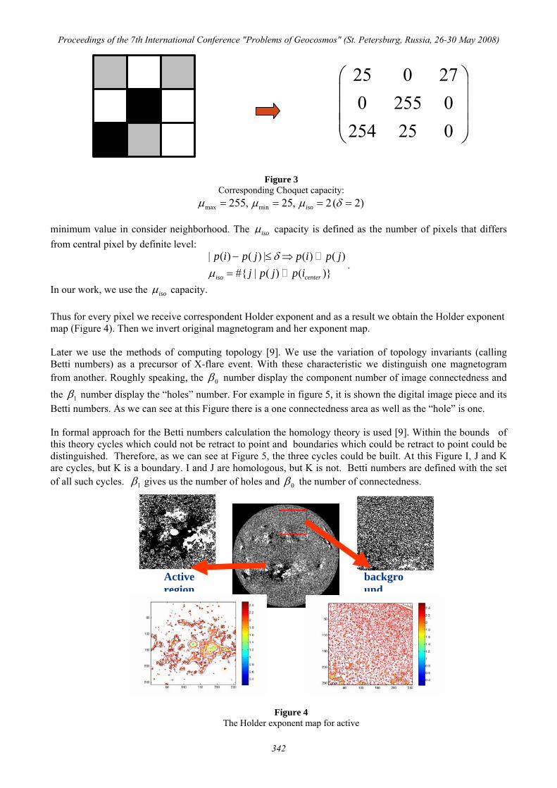
minimum value in consider neighborhood. The isoμ capacity is defined as the number of pixels that differs from central pixel by definite level:

| ( ) ( ) | ( ) ( )#{ | ( ) ( )}iso center

p i p j p i p jj p j p i

δμ

− ≤ ⇒=

.

In our work, we use the isoμ capacity. Thus for every pixel we receive correspondent Holder exponent and as a result we obtain the Holder exponent map (Figure 4). Then we invert original magnetogram and her exponent map. Later we use the methods of computing topology [9]. We use the variation of topology invariants (calling Betti numbers) as a precursor of X-flare event. With these characteristic we distinguish one magnetogram from another. Roughly speaking, the 0β number display the component number of image connectedness and the 1β number display the “holes” number. For example in figure 5, it is shown the digital image piece and its Betti numbers. As we can see at this Figure there is a one connectedness area as well as the “hole” is one. In formal approach for the Betti numbers calculation the homology theory is used [9]. Within the bounds of this theory cycles which could not be retract to point and boundaries which could be retract to point could be distinguished. Therefore, as we can see at Figure 5, the three cycles could be built. At this Figure I, J and K are cycles, but K is a boundary. I and J are homologous, but K is not. Betti numbers are defined with the set of all such cycles. 1β gives us the number of holes and 0β the number of connectedness.

25 0 270 255 0

254 25 0

⎛ ⎞⎜ ⎟⎜ ⎟⎜ ⎟⎝ ⎠

Figure 3 Corresponding Choquet capacity:

max min255, 25, 2( 2)isoμ μ μ δ= = = =

background

Active region

Figure 4 The Holder exponent map for active


342

We compute topological invariants both for original and inverted magnetograms and for original and inverted image of Holder maps. As a result we get four couple of such numbers. So, for active region which was observed during five days we obtain time series of Betti numbers with near 80 values. Results For exploration of the original magnetogram it was decided to investigate difference of corresponding Betti numbers for positive and negative images. We found out the distinction in variation of such difference for X-flare active region and flare-quiet active region. For flare quiet regions the differences oscillates near zero, but for flare active regions Betti differences were strongly above or under the zero level (Figure 6). From physical point of view such behavior signals that during the activity in region there is a prevalence of one polarity before another.

0 10 20 30 40-1000

-500

0

500

1000

1500

β ip -βin ; i

=0,1

# fits

β0p-β0

n

β1p-β

1n Figure 6

We find out the distinction in variation of such differences for X-flare active region and

flare-quiet active region. The difference oscillates near zero or in the various half

planes

0 10 20 30 40 50 60 70 80

100

200

300

400

500

600

700

β 0p -β0n

# fits

flare-quiet active region

0 10 20 30 40 50 60 70 80 90

-2500

-2000

-1500

-1000

-500

0

500

β 1p -β1n

# fits

X-flare active region

Figure 5 For given image digital piece 0β =1, 1β =1. Cycle I and J are

homologous. Cycle K retracts to point


343

The second result is connected with the investigation of Holder exponent maps. It was observed that 24 hours before the X-flare event there was a sudden change in Betti numbers for Holder maps images (Figure 7). Probably this confirms our assumption about magnetic flux buoyancy before the X-flare event and changes in the image topology. Conclusions The results obtained during the research are very interesting. The sudden change of gradient 24 hours before the X-flare events gives us evidence that we choose the right way of investigation. Further, of course we must increase the amount of exploration regions to provide more statistical significance results. The same is correct for effects of flare active or flare quiet regions. Naturally it is very useful to distinguish only by image whether region is flare active or flare-quiet. Reference 1. Turiel, A., N. Parga, The multi-fractal structure of contrast changes in natural images: from sharp edges

to textures, Neural Computation, (2000). 12, P.763-793 2. Huang J., D. Mumford, Statistics of Natural Images and Models, Proc. of the ICCV, (1999). № 1. P. 541–

547 3. Turiel, A., H. Yahia, C.J Pérez-Vicente, Microcanonical multifractal formalism — a geometrical

approach to multifractal systems: Part I. Singularity analysis, J. Phys. A: Math. Theor., (2007). 41. 015501

4. Falconer K. Fractal geometry. Mathematical foundations and applications. John Wiley & Sons. (1990). 5. Lawrence J.K., Ruzmaikin A.A., Cadavid A.C., Multifractal measure of the solar magnetic field, The

Astrophysical Journal, (1993). 417, P.805-811 6. Abramenko, V.I.: Multifractal analysis of solar magnetograms, Solar Phys., (2005), 228, P.29–42. 7. Conlon, P.A., P.T. Gallagher, R.T.J. McAteer et al., Multifractal Properties of Evolving Active Regions,

Solar Physics, (2007). 10.1007/s11207-007-9074-7 8. Kruglun, O.A., L.M.Karimova et al. Multifractal analysis and simulation of magnetograms of the full

Solar disk, Solnecno-Zemnaya Physika, (2007). 10. P.31-42 (in Russian) 9. Zomorodian, A. Topology for Computing. (2007) Cambridge Monographs on Applied and

Computational Mathematics

0 10 20 30 40 50 60 70 800

2000

4000

6000

8000

10000

12000 flare

β i; i

=0,

1

# fits

β0p(h)

β1n(h)

flare

Figure 7 We can see the sudden change 24 hours before the X-flare event


344

NONLINEAR ANALYSIS OF CAUSAL RELATIONSHIPS BETWEEN SOLAR AND GEOMAGNETIC TIME-SERIES BY MEANS OF SYMBOLIC

DYNAMICS

O. L. Oposhnyan1, D. I. Ponyavin1, N. G. Makarenko2

(1) Institute of Physics, St. Petersburg State University St. Petersburg, Russia, e-mail: [email protected], [email protected];

(2) Central (Pulkovo) Astronomical Observatory of RAN, St. Petersburg Russia, e-mail: [email protected]

Abstract. Causal relationships between geomagnetic indices aа and sunspot numbers were analyzed over a period 1868-2006. We studied nonlinear dynamics of time series by transforming them into symbolic words, according ordering relationships between records. The technique was tested first using logistic maps. It was shown that the method can be applied to detect regularities in a raw data and reveal intercorrelations of time series. Correlations between solar and geomagnetic dynamics are low and relatively best with delay of 3-4 years.

Introduction

Detection and estimation of interrelations between two dynamical systems using observable time series is a complex and ambiguous problem [1]. The linear analysis is focused on revealing linear correlations, and can lead to the false results, due to the noise of unknown origin. Besides that, linear relationships can simply be absent. In the present paper one of nonlinear tools, based on symbolical dynamics is tested [2, 4]. The main idea of this technique consists in transformation of time series into symbolic form by using order relationships between values. Each word of this text represents the definite code, taking into account the order ship between successive records [2, 3]. The primary advantage of this method is in admission of errors but only those which do not disturb the orderships in records. Moreover this technique allows use short time series. Further, it will be shown, that the method is quite sensitive to the level of connectivity between systems.

Symbolic technique

Let { } 1

nn i i

X x=

≡ - scalar time series, consist of n scores and }{ mXXXР ...21= , be a sequence of length

m extracted from nX . For instance, assume that first four indications are: { } ( )30,120,60,9043211 == XXXXP We will code this sequence by 4-h numerals of natural series being based on the attitude of the strict order between readouts (>, <)

( ) 3210120906030,30,120,60,901 pppppp=P According to this permutation this “word” is ( )0,3,1,21 =S . Thus, we have transformed sequence of four values to a symbolic code or a “word”. The following word is formed by shift of one record along the raw data, so that { }54322 XXXXP = etc. Numbers do not require a preliminary normalization as only their relations between successive values are important.


345

Test model To test model two raw data generated by the logistical equations [1] are used:

( )( )1

2 22

( 1) ( )(1 ( ))

( 1) ( )(1 ( )) ( )

x n x n x n

y n y n y n y n x n

λ

λ ε

+ = −⎧⎪⎨ + = − + −⎪⎩

(1)

with parameters ( ) ( )1 22,5; 3.2; 0 0 0.1x yλ λ= = = = . Coupling parameterε is introduced, number

of iterations 1000N = , word length 4m = . Occurrence rate of the words for each of time series was compared, by means of difference of corresponding histograms. It was supposed that the histograms differ slightly from each other in case of interaction of the systems. And, by contrary, difference is essential if systems are independent. The degree of difference of the histograms can serve as estimation of degree of coupling between systems. We notice that some of the words are frequently occurred or absolutely absent.

0132

0231

0312 1230

13202013 3102

0132

0132

0213

0213 13021320

3021 01320213

0312 2031

132013022031

2013

03121230

0312

0231

0231

0312

12301302

13202013

A B

С D

Figure 1. Histograms of occurrence rate of all possible words of time series produced by system (1): A. At parameter ε = 0 (no coupling); B. ε = 0.6; C. ε=0.8; D. ε=1.1 (strong interaction). The sum of bars of difference histograms for various values of ε is presented in Table 1.

Table 1 Parameter of coupling, ε Sum, ∆

ε = 0 ∆ =100 ε =0.6 ∆ = 43 ε =0.8 ∆ = 16 ε =1.1 ∆ = 6

From the Table 1 it follows that the value of sum ∆ depends strongly on the interaction between systems.


346

Application to the real-world data We have used annual means of geomagnetic indices аа1 and sunspot numbers22 for the period 1868-2006. It is known, that the geomagnetic cycle is not completely synchronized with 11-year cycle of solar activity. The geomagnetic cycle in average lasts a sunspot cycle. At the same time the recurrent geomagnetic activity during a declining phase of solar cycle correlates with subsequent solar cycle [5] that can is used in forecasting of solar activity [6]. Thus, the dynamics of geomagnetic activity are controlled by a current cycle and, apparently, correlates with the following cycle. Herewith we compare the time series of solar and geomagnetic activity by shifting sunspot series back relative to geomagnetic records. In case of shifts for 3 and 4 years the sum of bars of difference histograms became a minimal. A similar result has appeared for shifts of 2 and 5 years.

0123

0213 1023 2130 3012

3210

3201

Аa-Volfs_without lag

0123

02131023 2130

21032310

3102

3210

3201

А 12a-Volfs_with lag years

0123

02131023

21303012

3210

3201

А a-Volfs_with lag 3 years

0123

02131023 2130

3012

3210

3201

А 6a-Volfs_with lag years

Figure 2. A difference of frequency histograms of sunspot and geomagnetic time series for various shifts. In the Table 2 the sum of column differences of histograms for various shifts are presented.

Table 2 Shift, years Sum, ∆

without shift ∆ =98 1 year ∆ =99 2 years ∆ =96 3 years ∆ =92 4 years ∆ =92 5 years ∆ =96 6 years ∆ =94

12 years ∆= 99 1 http://www.wdcb.rssi.ru/stp/data/geomagni.ind/aa/aa/ 2 http://www.ngdc.noaa.gov/stp/SOLAR/ftpsunspotnumber.html


347

Conclusions

• Symbolic analysis can be applied for revealing of nonlinear coupling between dynamical systems.

• Correlations between sunspot and geomagnetic dynamics are low. The best correspondence is observed at delay 3-4 years of geomagnetic activity relative to sunspot time series.

Bibliography

1. Bezruchko B.P., D.A. Smirnov. Mathematics modeling and chaotic time series. Saratov State Univ.

Press, 2005, 320 p. 2. Daw C.S., C.E.A. Finney, E.R.Tracy. A review of symbolic analysis of experimental data, Rev.

Scientific Instruments, 2003, vol. 74, 915-930. 3. Bandt C., B. Pompe. Permutation entropy: a natural complexity measure for time series, Phys. Rev.

Lett., 2002, vol. 88, 174102. 4. Monetti R., W. Bunk, F. Jamitzky. Characterizing synchronization in time series using information

measures extracted from symbolic representations./ arXiv: 0804.4634. 5. Ohl A.I., G.I. Ohl. A new method of very long-term prediction of solar activity, In: Solar-Terrestrial

Predictions Proc., Boulder Colo., 1979, vol. 2, 258-263. 6. Hathaway D.H., R.M. Wilson. Geomagnetic activity indicates large amplitude for sunspot cycle 24,

Geophys. Res. Lett., 2006, vol. 33, L18101, doi:10.1029/2006GL027053.


348

MULTISCALE INTERMITTENCY IN PHYSICS AND PHYSIOLOGY

V.M. Uritsky 1 and N.I. Muzalevskaya 2 1University of Calgary, AB, Canada, e-mail: [email protected];

2 St. Petersburg State University, St Petersburg, Russia

We review our recent results in multiscale intermittency analysis of correlated stochastic behavior in complex natural systems. The approaches discussed include spatial higher-order structure functions, fractal time-series analysis methods, as well as spatiotemporal decomposition of time-dependent turbulent fields into sets of discrete dissipation events. These approaches are illustrated by several examples, including flaring activity in the solar corona, electron precipitation dynamics in the auroral zone, and multiscale fluctuations in human cardiovascular system. In each application, the proposed intermittency measures provide significant new information about the scaling regimes, correlation patterns, and the underlying thermodynamic states of studied systems.

Introduction

This paper summarizes recent advances in the applications of methods of dynamical complexity to complex physical and physiological systems. Due to the size limitation, it primarily focuses on original contributions by the authors. To compensate for this bias, references to more comprehensive review articles will be given throughout the text. The main outcome of our analyses is an innovative methodology relating statistical properties of intermittent processes in natural systems with their large-scale, low-dimensional behavior. This conceptual link provides an opportunity to better understand the relationship between stochastic and deterministic dynamics of complex systems, to classify their internal instabilities as well as the response to an external driver, and to predict future changes.

The paper starts with a brief systematic overview of computational approaches for dealing with complex intermittent signals. Next, we present two examples of intermittent complexity and critical avalanching in turbulent space plasmas. Our third example (stochastic aspects of heart rate variability) features intermittency beyond physics, and shows diagnostic capabilities of multiscale complexity analysis in medical applications. Mathematical details will be kept at a minimum, with the emphasis placed on the interpretation of the processes under study.

Spatial and temporal measures of intermittency

Multiscale intermittency is a manifestation of dynamical complexity in driven spatially distributed nonequilibrium systems. Self-organized criticality (SOC) and intermittent turbulence (IT) represent two major paths to this dynamical state [3, 29]. In the classical fluid turbulence, scaling is often associated with a hierarchical structure of eddies extending over the inertial range, while in SOC, avalanches of localized instabilities organize the system toward a steady state exhibiting long-range correlations up to the system size. In both scenarios, intermittency implies strongly non-Gaussian behavior of studied variables which undergo frequent and sudden changes often resulting in “fat-tailed” distributions functions such as those descried by the Levy statistics. The statistical structure of intermittent signals also involves long-range (non-exponential) autocorrelations observed over many decades of temporal and spatial scales. The hierarchy of memory effects behind this structure is usually described by fractal and multifractal models, and it tends to exhibit nonstationary properties when studied over restricted time intervals.

The nontrivial statistical signatures of intermittent signals makes it difficult to obtain their quantitative parameters. Slow convergence of sample estimates, undefined statistical moments, unresolved low-frequency spectral components, poor reproducibility of results, broad confidence intervals, and other complications are very common when such signals are analyzed by standard statistical tools. These problems reflect principle limitations of classical probability theory which, according to its underlying axiomatics, is not intended to deal with cooperative stochastic processes with many interacting degrees of freedom, and can only tackle their simplified counterparts obtained as expansions about solutions that disregard the interactions.

A more adequate framework for dealing with multiscale intermittent processes is offered by the modern theory of dynamical complexity which aims at a quantitative analysis and physical interpretation of correlated stochastic behaviors in nonlinear interactive systems. The data analysis tools designed in this actively growing research field have been successfully applied to a variety of problems unsolvable by classical methods.


349

Spatial intermittency. A large group of complexity methods is based on a generalization of the classical turbulence theory to the case when the dissipation field is represented by an inhomogeneous spatially correlated multifractal set [1, 29]. Following the ideas originated by A.N.Kolmogorov (1941), such irregular turbulent fields can be characterized by a collection of (unsigned) structure functions Sq (l) = ⟨| A(x) – A(x + l) |q ⟩x,|l|=l, where A is the variable under study (velocity, magnetic field, Elsässer variables, or a relevant passive scalar), x – spatial coordinate, l – displacement vector, q – the order of the structure function. It is expected that each structure function varies with the spatial scale as Sq ~ lζ (q). The ζ (q) dependence plays an important role in identifying the nature of the turbulent fluid. It takes the linear ζ =q/3 form for the non-intermittent (homogeneous) 3D turbulence, and exhibits a more complicated scaling in intermittent systems [19]. In certain cases, the so-called extended self-similarity (ESS) analysis is also applied in which Sq is plotted versus a reference structure function (e.g. Sq (S3)). Such normalization yields relative values of ζ exponents, which is sufficient for validating many turbulent models.

Temporal intermittency. The second group of tools that are commonly used to study intermittent systems is fractal and multifracal time series analysis methods. A time-series generalization of the structure function analysis is straightforward, and it provides a spectrum of temporal ς exponents. Some other methods are the detrended fluctuation analysis, wavelet transforms, methods relying on singular value decomposition of temporal signals in the vector space, a variety of fractal and multifractal tools, and adaptations of Fourier power spectral analysis for processing nonstationary signals [8, 11, 22]. The intermittency measures provided by these methods are scaling exponents and scaling functions describing the relationship between statistical memory effects across different time scales. Some of these methods are applicable to spatially distributed data fields and can be used as auxiliary tools for examining inhomogeneous scaling of turbulent processes.

Intermittency in space-time. The third group of methods addresses the coupling between spatial and temporal aspects of the behavior of the complex system. This coupling is important because in many situations, complex processes simultaneously evolve in space and in time, and the interaction between the two is farily nontrivial. Paradigmatic examples of spatiotemporal intermittency in nonlinear systems with spatially extended degrees of freedom are critical avalanches of instabilities in sandpile SOC models and bursty localized energy dissipation in high-Reynolds number fluids. In our earlier works [23, 26], we have developed an approach for quantifying such manifestations of complex intermittent behavior which are abundant in nature and simulations. The approach is based on spatiotemporal decomposition of a continuous time-dependent turbulent field into a collection of discrete dissipation events composed of contiguous spatial regions of propagating activity. This nonlinear decomposition provides a detailed representation of the intermittent component in the studied dynamics in terms of its most essential statistical and topological features, while significantly reducing the amount of stored information. It also allows to selectively address different classes of intermittent disturbances based on multidimensional filtering criteria.

Example 1: Solar corona

Dissipation mechanisms in the solar corona are activated by changes in the configuration of its magnetic field which has distinct IT signatures [1]. Convection of magnetic fields leads to radiative transients, plasma jets, and explosive events known as flares. The latter are associated with spatially concentrated release of magnetic energy accompanied by localized plasma heating up to temperatures of 107 K, and can be observed by short-wavelength light emission. Flares tend to appear at irregular times and locations and exhibit broadband energy, size, and lifetime statistics with no obvious characteristics scales. This behavior is often interpreted as a signature of SOC [5].

We have studied time series of full-disk digital images of the corona taken by the extreme ultraviolet imaging telescope (EIT) on board the SOHO spacecraft in the 195A° wavelength band corresponding to the Fe XII emission. The data included two observation periods: 3240 images from a solar minimum period and 4407 images from a solar minimum period, with a typical time resolution of 13.3 min. The EIT luminosity was analyzed as a function of time and position on the image plane. To characterized spatial intermittency of SOHO EIT images, we computed higher-order structure functions in which the luminosity was used as the relevant field variable A. To identify SOC avalanches, we used the spatiotemporal decomposition method [23] resolving concurrent events. Avalanching regions were identified by applying an activity threshold representing a background EUV flux. Contiguous spatial regions above the threshold were treated as pieces of evolving dissipation events, and their statistics have been evaluated.

Our results suggest that the intermittency in the corona has a fundamental impact on the dissipation mechanism in this system (Fig. 1). The main energy resource for the flaring activity is the photospheric magnetic field. Its complex, highly fragmented spatial geometry contributes to the intermittent scaling of the


350

radiated UV flux described by a nonlinear ζ (q) dependence. The model by Müller & Biskamp [19] which provides a reasonable fit to our data describes IT in an ideal MHD plasma resulting from direct energy cascades. On the hand, the power-law statistics of energy release events suggests that a significant fraction of plasma energy is liberated in the form of inverse cascades characteristic of SOC systems. The apparent contradiction cannot be resolved in frames of existing coronal heating theories, and can be a starting point of building a more general framework which would incorporate a bi-directional energy cascade associated with collaborative IT and SOC scenarios.

(a)

(b)

(c)

Fig. 1. Coexisting signatures of IT and SOC in the activity of solar corona [26]. (a) Higher-order spatial structure functions of the EIT luminosity. The inset shows ESS plots exhibiting broad-band power-law scaling. (b) Relative (ESS-based) structure function exponents compared to turbulence models due to Kolmogorov (K41), She & Leveque (SL) and Müller & Biskamp (MB) [19]. (c) Energy distributions of coronal avalanches during periods of solar minimum and maximum showing robust power-law scaling indicative of SOC. The solar min distributions are shifted for easier comparison. Different colors represent several activity thresholds used to identify the avalanches.

From a more practical point of view, it is evident that the process of coronal dissipation can not be predicted without taking into account its stochastic intermittent component which seems to control the primary energy conversion in the turbulent solar plasma [1]. One way to model future dynamical transitions in the corona is to reconstruct its magnetic network and to run a SOC algorithm that would reconnect magnetic loops thus producing flaring events. Such simulation would help reveal unstable magnetic topologies responsible for major flares, coronal mass ejections, and other space weather phenomena.

Example 2: Earth’s magnetosphere

The necessity of using complexity tools in magnetospheric research has fundamental reasons. Unlike solar wind turbulence which at the distance 1 AU from the coronal source can be considered as "fully developed", many, if not all, magnetospheric processes are usually in a highly intermittent transient state [4, 28]. Sporadic bursts of energy dissipation, localized acceleration processes, non-steady driving, strongly inhomogeneous fluctuations involving both kinetic and MHD domains, and other forms of transient stochastic activity are fairly common in magnetospheric plasma. This messy, non-steady turbulent dynamics can not be adequately described by any of the established turbulence theories. However, it naturally fits in a more general framework of multiscale dynamical complexity providing a rich variety of methods for dealing with non-classical stochastic processes such as those observed in Earth's magnetosphere [7, 27].

Magnetospheric substorms are accompanied by a variety of intermitted processes in the auroral zone. Soon after the development of the basic substorm phenomenology, it has been realized that the nighttime auroral oval is not a simple latitudinally bound distribution of emission brightness and electric currents. The activity of this part of the ionosphere is extremely complex, and it incorporates a multitude of effects reflecting different conditions on the solar wind - magnetosphere - ionosphere coupling system. Examples of these are substorm expansion onsets, pseudobreakups, steady magnetospheric convection events with or without substorm activity, bursty bulk flows, sawtooth events, and other processes [2, 6, 21]. Despite a remarkable diversity of physical phenomena involved in the magnetospheric response to the solar wind driver, the output energy dissipation flux as estimated from particle precipitations in the nighttime aurora tends to cluster in intermittent spatiotemporal bursts obeying simple and nearly universal scale-free statistics [10, 12, 23].


351

The term ”scale-free” has been coined in statistical mechanics of turbulent and/or critical phenomena to describe correlated perturbations with no characteristic scales other than the scales dictated by the finite size of the system, as opposed to scale-dependent perturbations reflecting physical conditions that vary across different scales [29]. Considered in the context of other geophysical processes, the nighttime auroral activity provides one of the most impressive examples of scale-free behavior in Nature. Thus, the energy probability distribution of electron emission regions as seen by the POLAR satellite exhibits power-law shape over about 6 orders of magnitude [23]. By combining POLAR data with ground-based TV observations [10], the power-law scaling range has been extended up to 11 orders of magnitude (Fig. 2). The consistency of the power-law slopes obtained from high-resolution ground-based auroral observations and those characterizing POLAR ultra-violet imager (UVI) data reveals an extremely wide range of power-law scaling of energy dissipation in the nighttime magnetosphere.

(a)

(b)

Fig. 2. (a) A diagram explaining the idea of spatiotemporal tracking of auroral emission regions in time series of POLAR UVI frames (LBH-long filter). (b) Power-law probability distributions of electron emission areas obtained from ground-based all-sky camera data (triangles) and the POLAR UVI observations (squares) [10, 23].

It is worth noting that these scale-free statistics represent long-term ensembles-averaged properties of nighttime magnetospheric disturbances, and they can mask a more complex dynamics on the level of specific plasma sheet structures responsible for the generation of various forms of auroral precipitations. Our recent results [24, 25] confirm the causal relationship between the auroral precipitation statistics and the non-uniform morphology of the central plasma sheet. They show that the inner and the outer plasma sheet regions are responsible for distinct scaling modes of the auroral precipitation dynamics which can a manifestation of two competing substrm scenarios represented by the current disruption and the midtail magnetic reconnection models [13, 20]. Exploring such second-order scaling effects could help build a more solid theoretical link between the statistical and dynamical plasma descriptions, evaluate predictability of different classes of magnetospheric disturbances, and obtain statistical guidelines for designing future space missions targeted at multiscale plasma phenomena.

Example 3: Human heart rate variability

This section illustrates an intermittent stochastic behavior in a quite different system – the system of human homeostasis, monitored by the low-frequency component of heart rate variability (HRV) [9,17]. HRV is the temporal variability of the beat-to-beat RR-interval in human electrocardiogram which exhibits distinct intermittent properties in the frequency range 10–5 − 10–2 Hz [14]. In many cases, this variability is described by the power-law 1/f β dependence of Fourier power spectral density on the frequency f [9]. Typically, 1/f β HRV spectra with constant β are observed in healthy people, whereas pathologies and malfunctions are associated with more complex forms of spectral behavior. The connection between the broken fractality and the disease [15-18, 22] indicates a possibility of using 1/f β fluctuations for the purposes of clinical diagnostics, and stimulates further investigation of this phenomenon. In our previous studies, we have explored fractal and multifractal properties of HRV using a variety of time series analysis tools [15,17,18]. The results have confirmed that the low-frequency HRV is a sensitive marker of homeostatic processes. Here we present new results showing that intermittency measures of HRV can be used for early identification of pathological conditions.

In addition to power-law spectral exponent β, we consider two intermittency parameters (a and T) describing nonstationary behavior of standard deviation in HRV signals as explained in Fig. 3. In medical applications, extreme abnormal values of σ and β are informative state parameters. The interpretation of σ is largely empirical and is carried out on the individual basis for different sets of symptoms. Earlier, we have proposed an interpretative system for σ understanding measurements in the SOC region of HRV regulation


352

where the standard deviation plays a role of stochastic magnitude of dissipation losses under the conditions of fractal symmetry of homeostatic dynamics (σ i = σ F =σ ). Since the constant magnitude is a signature of the stationary balance between the supplied and dissipated regulatory energies, we suggest that in general, the parameter σ F can be used as a sensitive statistical marker of the current amount of available regulatory energy characterizing fractal self-organization of HRV for a broad range of physiological conditions. Distortion of fractal symmetry of HRV occurring outside the SOC region [17] reduces the scaling range of fractal R-R fluctuations, decreases available energy resource, and increases nonstationarity and intermittency in HRV, which requires a substantially different approach to interpreting σ and β measurements.

[ ]( ) { }

normF

F

normF

F

iF

Nt

ttNtttti

RRRRaTa

ffSRRRRN

i

iii

1;:measuresncy Intermitte

)(|min,1

1 2

,

σσσ

σσσ

σσσ β

−≡=−=

∝=−+

= −+

=+∈∑

Fig. 3. Analysis of intermittency of HRV signals. The HRV sample is divided into subintervals of length N characterized by different degree of intermittency as measured by local estimates σ i of the standard deviation σ. The subinterval with the smallest σ =σF describes the “laminar” fractal component of HRV and is used to evaluate the intermittency indices a and T. ⟨RR⟩norm is the normalized age-adjusted average value of the R-R interval.

Table 1. Intermittency measures of HRV for several cardiovascular disorders ( n – number of cases )

To evaluate the intermittency of HRV signals, we use two constituents of the standard deviation – its

stationary fractal component σ F as well as the nonstationary component σ –σ F. Each component has its own diagnostic value, while their balance which is reflected by the definitions of a and T (see Fig.3) is a sensitive measure of turbulent intermittency in the HRV signal. Both a and T are small (of the order of 0.1) for healthy unperturbed homeostatic regulation, and they gradually increase with an increase of mental concentration and emotional load. Pathological conditions (Table 1) are characterized by much higher levels of a and T

n a <RR>norm T Physiological characteristics

Pathoadaptation dynamics prior to onsets of cardiac arrhythmias 1.1 11 1.40 1.20 ± 0.06 1.27 ± 0.30 One week before an atrial fibrillation (AF) event 11 4.20 1.19 ± 0.08 3.60 ± 0.20 3 days before AF 11 7.30 1.37 ± 0.04 5.30 ± 0.10 1 day before AF 1.2 7 1.40 0.89 ± 0.03 1.60 ± 0.40 Prior to atrial palpitation (AP), sinus tachycardia 1.3 9 1.50 1.18 ± 0.04 1.30 ± 0.30 Prior to AP, sinus bradycardia 9 7.40 1.35 ± 0.02 5.50 ± 0.20 Same, 1 day before AP event Myocardial infarction, case 1 2.1 1 4.26 0.82 5.19 Acute condition, first week 1.10 0.93 1.18 3 weeks later 0.54 0.98 0.56 4 months later 0.24 1.07 0.22 Rehabilitation Myocardial infarction, case 2 2.2 1 >10 0.78 >10 Acute condition 4.60 0.86 5.35 Intensive care (reanimation) >10 0.79 >10 Critical condition Ischemic brain stroke, case 1 3.1 54 2.81 1.08 ± 0.05 2.60 ± 0.60 Acute condition 54 0.86 1.08 ± 0.02 0.79 ± 0.29 Before discharge from hospital Ischemic brain stroke, case 2 3.2 14 3.45 0.96 ± 0.03 3.59 ± 0.73 Acute condition 12 7.12 0.80 ± 0.06 8.80 ± 0.90 Coma


353

indicating a significant increase of HRV intermittency in disease. For T >10, self-organization homeostatic processes necessary to maintain normal HRV are effectively replaced by random intermittency, a signature of a severe medical condition.

Our new findings strongly suggest that the intermittency measures a and T can be used as empirical proxies for the available energy resource of the adaptation system. In pathological conditions, this resource significantly decreases as reflected by abnormal a and T values. Considering inherent nonstationarity of HRV signals observed for such conditions, it is also evident that the physiological interpretation of the standard deviation of R-R intervals – the quantity most widely used in clinical applications [14] – must be adjusted for different diseases and adaptation scenarios, depending on the relative contribution of the fractal (1/f β) and the intermittent (a, T) variability to the studied stochastic signal.

Concluding remarks

We have provided several illustrative examples in which intermittency measures of seemingly random signals carry new information about system-level properties of studied processes. The common element of the complexity techniques that have been invoked in this context is their ability to characterize multiscale hierarchy of studied physical or physiological processes. This methodological advantage proves quite valuable when the macroscopic behavior is critically dependent on cross-scale interactions. The latter can be implemented in a real-space of spatially distributed geophysical systems, or in an abstract state-space of of complex dynamical system such as the system of human homeostasis. In both cases, adequately chosen intermittency measures can be used to obtain significant new information about the scaling regimes, predictability, correlation pattern, and functional stability of the studied system. References 1. Abramenko,V. I. and V. B. Yurchyshyn, Astrophys. J., 597: 1135, 2003. 2. Angelopoulos, V. et al. Phys. Plasmas, 6(11):4161–4168, 1999. 3. Bak, P. et al., Phys. Rev. Lett., 59: 381, 1987. 4. Borovsky, J. E. et al. J. Plasma Phys., 57:1–34, 1997. 5. Charbonneau, P. et al. Sol. Phys., 203(2):321–353, 2001. 6. Donovan, E. et al. J. Atmos. Sol. – Terr. Phys., 68(13):1472–1487, 2006. 7. Freeman, M. P. and N. W. Watkins. Science, 298(5595):979–980, 2002. 8. Glenny, R.W. et la. J. Applied Physiology, 70(6): 2351-2367, 1991. 9. Kobayashi, M. and T. Musha. IEEE Trans. Biomed. Eng.,29:456–457,1982. 10. Kozelov, B.V. et al. Geophysical Research Lett., 31(20 ), 2004. 11. Kumar, P, and FoufoulaGeorgiou, E. Reviews of Geophysics, 35(4): 385-412, 1997. 12. Lui, A. T. Y. J. Atmos. Sol.-Terr. Phys., 64(2):125–143, 2002. 13. Lui, A. T. Y. Space Science Rev., 95(1-2):325–345, 2001. 14. Malik, M. et al. Circulation, 93:1043–1065, 1996. 15. Muzalevskaya, N.I and V.G. Kamenskaya, Human Physiology, 33(2): 179-187, 2007. 16. Muzalevskaya, N.I et al., Zhurnal Nnevropatologii i Psikhiatrii Imeni Korsakova, 7: 54-58, 2002. 17. Muzalevskaya, N. I. and V. Uritsky, In: Telemedicine: the 21st Century Informational Technologies, St.

Petersburg: Anatolia Press, 209–243, 1998. 18. Muzalevskaya, N.I. and V.M. Uritsky, In: Longevity, Aging and Degradation Models in Reliability, Public Health,

Medicine and Biology, 1: 283–297, St.Petersburg: SPbGTU Press, 2004. 19. Müller, W.-C. and D. Biskamp, Phys. Rev. Lett., 84: 475, 2000. 20. Ohtani, S. I. Space Science Rev., 113(1-2):77–96, 2004. 21. Sergeev, V. A. et al. J. Geophys. Res. – Space Phys., 98(A10):17345–17365, 1993. 22. Stanley, H. E. et al. Physica A, 270:309–324, 1995. 23. Uritsky, V. M. et al. J. Geophys. Res. – Space Phys., 107(A12):1426, 2002. 24. Uritsky, V. M. et al. Ann. Geophys. (submitted), 2008. 25. Uritsky, V. M. et al. Geophysical Research Lett., 35:L21101, 2008. 26. Uritsky, V.M.. et al., Phys. Rev. Lett., 99: 025001-1 – 025001-4, 2007. 27. Valdivia, J. A. et al. Advances in Space Research, 35(5):961–971, 2005. 28. Voros, Z. et al. Space Science Rev., 122(1-4):301–311, 2006. 29. Warhaft, Z. Proc. National Acad. Sciences United States Am., 99:2481–2486, 2002. 30. Waldrop, M. M. Complexity: The Emerging Science at the Edge of Order and Chaos. New York: Simon &

Schuster, 1992.


354

FRACTAL CHARACTERISTICS OF THE SOLAR AND MAGNETOSPHERIC ACTIVITIES AND FEATURE OF THE AIR

TEMPERATURE DYNAMICS

O.D. Zotov1, B.I. Klain1

1Geophysical Observatory Borok, IPE, RAS, Borok, Russia, e-mail: [email protected]

Abstract. Series of daily values of solar activity (Wolf's numbers), magnetospheric activity (Ap-index), air temperature and global seismic activity for 1930-2000 were analyzed. Dynamics of the Hurst exponent and dynamics of the average for all series of the data were defined. The comparative analysis of geophysical environments characteristics has been made. Correlation in dynamics of the fractal dimensions of investigated series was found. Feature near 1960 year in dynamics of the Sun activity and the magnetospheric activity was found. It was revealed that till 1960 dynamics of the air temperature does not correlate with dynamics of the magnetosphere activity, and after 1960 high correlation is observed. The hypothesis probably explaining features of investigated processes dynamics is considered. The change of a chaotic mode of the Sun activity there was near 1960. It has led to change of the geospheres dynamics character. This phenomenon can be interpreted as the noise induced phase transition in the Earth’s system.

The view on a problem of Solar-Terrestrial interaction is that the Earth as the complex system of

cooperating geospheres is a nonlinear system with own noise and the external stochastic influence caused by non-stationary processes on the Sun. We shall consider long period variations (duration of several tens years) of solar activity parameters of chaotic component, variations of amplitudes and fractal dimensions of geomagnetic activity and air temperature.

Data. Series of daily values of solar activity (SSN - Sun Spot Numbers) [www.wdcb.ru] and solar activity chaotic component (SSN_Ch), geomagnetic (magnetospheric) activity (Aр-index) [ww.wdcb.ru], air temperature (Т) for six meteorological stations in Russia along Volga-river (Fig.1) from Astrahan to Vologda [www.meteo.ru] and geophysical parameters for other geospheres for 1930-2000 were analyzed.

Fig. 1. Six meteorological stations in Russia along Volga-river.


355

mailto:[email protected]

Method. For all series we calculated and analyzed: dynamics of sliding average ( for example Ap with letter M – Ap M ), sliding windows 365 points (1 year) and step 50 points (50 days); dynamics of sliding parameter of Hurst or Hurst exponent ( for example SSN H ), windows 365 points (1 year), step 50 points (50 days). Hurst's parameter is interpreted as a fractal dimension; dynamics of sliding correlation coefficient (Ccor), windows 3650 points (10 years), step 365 points (1 year); dynamics of cumulative deviation from the average or difference integral curve (for example iTM); Algorithm of calculation of cumulative deviation from the average:

, ∑=

−=k

imik xxy

1)(

where ∑=

=n

iim x

nx

1

1 and n – a number of the points in series.

Note. Dynamics of magnetospheric activity (Ap M) has features which are not present in dynamics

of solar activity (SSN M). Dynamics Ар M contains 11-years component of dynamics of solar activity, but has essential differences. They are visible in details with characteristic time scale of several years order. Namely: local minimum Ар when SSN having maximum or maximum Ар on a SSN declining phase is observed. Dynamics of SSN amplitude does not define dynamics of amplitude of magnetospheric activity, at least, with time scales of solar cycle duration (Fig. 2a).

At Fig. 2b we see feature of Ccor dynamics: its sharp declining begins in area of 1960.

Fig. 2. a - dynamics of sliding average of solar SSN M and magnetospheric Ap M activities, b - dynamics of sliding correlation coefficient Ccor between SSN M and Ар M. The yellow vertical columns indicate the feature in area of 1960 here and further. Analysis: SSN – Ap.

Dynamics of the sliding Hurst exponent for solar (SSN H) and magnetospheric (AP H) activity show on Fig. 3a. We see no correlation between these processes. At Fig. 3b we see good correlation between dynamics of cumulative deviation from the average Hurst exponent for solar and magnetospheric activity. Note the dynamics of i SSN H and i AP H curves means that amplitude of low-frequency components in spectra of solar and magnetospheric activity chaotic components was more till 1960 then after 1960. Fig. 3c shows a burst of amplitude of solar activity chaotic component near 1960 also.


356

Fig. 3. a - dynamics of the sliding Hurst exponent (H) for solar (SSN H) and magnetospheric (AP H) activity, b - dynamics of cumulative deviation from the average Hurst exponent for solar (i SSN H) and magnetospheric (i AP H) activity, c - dynamics of cumulative deviation from the average of solar activity chaotic component (i SSN_Ch M).

We observe the feature of dynamics of chaotic component of solar and magnetospheric activity around 1960 year.

Analysis: Ap – Temperature. We see some high correlation between dynamics of cumulative deviation from the average of chaotic components for all meteorological stations. Fig. 4a shows data for three stations only. Data of the other three stations have similar dynamics.

Fig. 4. a - dynamics of cumulative deviation from the average (Hurst exponent) for air temperature i Т H, b - dynamics of sliding average amplitudes Ap and T, c - dynamics of cumulative deviation from the average amplitudes Ap and T.


357

Also we see feature in dynamics of chaotic component of temperature: its sharp declining begins in area of 1960 (Fig. 4a). Simultaneously we see an appearance of correlation between an average amplitude of Ap-index and T near 1960 year (Fig.4b and Fig.4c).). We see low correlation till 1960 and after 1960 high correlation (see also Fig. 5b)

What happens? What has occurred in dynamics of geospheres (correlation between magnetosphere activity and air temperature after 1960)? How this phenomenon can be explained?

Correlation in dynamics of the fractal dimensions of the investigated series was found. Feature near 1960 year in dynamics of the Sun activity chaotic component and the magnetospheric activity also was found. The dynamics of the air temperature does not correlate with dynamics of the magnetosphere activity till 1960 and high correlation is observed after 1960.

First hypothesis: The change of a spectral structure (Hurst exponent) and burst of amplitude of chaotic mode of the Sun activity was near 1960. It has led to change of the geospheres dynamics character. The phenomenon can be interpreted as the noise induced phase transition in the Earth’s system.

Second hypothesis: The technogenic influence on geospheres connected with a significant intensification of nuclear tests and the beginning of a space age has sharply increased in area of 1960. There is other possible reason of effect of correlation changes between temperature and magnetic field in this situation, namely, influence of the anthropogenous factor.

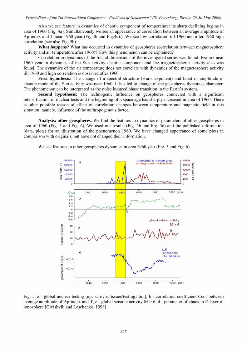
Analysis: other geospheres. We find the features in dynamics of parameters of other geospheres in

area of 1960 (Fig. 5 and Fig. 6). We used our results (Fig. 5b and Fig. 5c) and the published information (data, plots) for an illustration of the phenomenon 1960. We have changed appearance of some plots in comparison with originals, but have not changed their information.

We see features in other geospheres dynamics in area 1960 year (Fig. 5 and Fig. 6).

Fig. 5. a - global nuclear testing [npc.sarov.ru/issues/testing.html], b - correlation coefficient Ccor between average amplitude of Ap-index and T, c - global seismic activity M > 6, d - parameter of chaos in E-layer of ionosphere [Givishvili and Leschenko, 1998]


358

Fig. 6. a - space launches and dynamics of ozone layer (www.evolunity.ru/books/dmitriev/TechOnNature), b -temperature in Sikhote-Alinsky reserve (www.tigers.ru/res/klm/klimat.html), c -equivalent height of the F-layer of ionosphere (www.kosmofizika.ru/irkutsk/kok/TMP183.htm).

Conclusion. Simultaneous changes in geospheres (magnetosphere, ionosphere, stratosphere, atmosphere and lithosphere) in area of 1960 are the real geophysical phenomena.

We are still far from clear understanding the concrete physical mechanisms of the Solar or human impacts on the Earth’s geospheres.

First hypothesis: feature in geospheres dynamics near 1960 year is phenomenon of the solar noise induced phase transition in the Earth’s system of geospheres.

Second hypothesis: feature in geospheres dynamics near 1960 year is phenomenon of the human impacts.

The question of a source of changes in geospheres in area of 1960 for the time present remains still opened. It is not excluded also that both sources act on geospheres simultaneously. It is clearly we must consider all anthropogenic influence when analyzed the long period dynamics of various parameters of geospheres, and especially by search of correlations with solar activity.

We would like to thank Prof. A.V. Guglielmi for his interest to this work and for some valuable remarks. This work was supported by Basic Research Program no. 16 “Changes in the Environment and Climate: Natural Catastrophes” of the Russian Academy of Sciences and Russian Foundation for Basic Research, project nos. 06-05-64143.

REFERENCIS.

Givishvili, G.V., L.N. Leshchenko (1998), Rhythms in ionosphere and in upper atmosphere of the Earth, Atlas of temporal variation of natural, anthropogenic and social processes. Volume 2. Cyclical dynamic in the nature and the society. M. Scientific World. 432 с.


359

http://www.evolunity.ru/books/dmitriev/TechOnNature

http://www.tigers.ru/res/klm/klimat.html

http://www.kosmofizika.ru/irkutsk/kok/TMP183.htm

STOCHASTIC RESONANCE IN THE EARTH’S MAGNETOSPHERE

O.D. Zotov1, B.I. Klain1, N. A. Kurazhkovskaya1

1Geophysical Observatory Borok, IPE, RAS, Borok, Russia, e-mail: [email protected]

Abstract. The relationship between dynamics of average daily values of solar activity chaotic component (Sunspots number) and dynamics of average daily values of the Earth magnetospheric activity (Ap-index) has been investigated. The magnetosphere can be viewed as the system which is in a metastable state. The influence of external noise on such systems will lead to occurrence of casual switching between attractors of the system. As a result the geomagnetic activity will be defined by properties of the external noise. It is shown that exactly chaotic component of the solar activity defines features of magnetospheric activity dynamics. It is shown that using the method of nonlinear dynamic scanning it is possible to explain the dynamics of magnetosphere by the effect of a stochastic resonance. The simple model which explains statistics of the Ap-index has been suggested. In this model the Gaussian noise (the solar activity chaotic component) has an influence on an input of the system (magnetosphere). At the output of the system (Ар-index) the distribution of the noise has properties of the so-called “heavy tail”. Keywords: solar activity, magnetosphere, stochastic resonance.

This paper deals with the problem of solar activity influence on the Earth magnetospheric activity.

Series of daily values amplitude of solar activity (SSN - Sun Spot Numbers - Wolf's numbers) [www.wdcb.ru] and geomagnetic (magnetospheric) activity (Aр-index - Ap) [www.wdcb.ru] (Fig. 1a) for 1930-2000 were analyzed.

Fig.1. a - daily values dynamics of solar activity SSN and Earth magnetospheric activity Ap, b - dynamics of average amplitudes of solar SSN_M and magnetospheric activity Ap_M, c - dynamics of chaotic component amplitude SSN_Сh, d - dynamics of average amplitudes of chaotic component SSN_Ch_M and SSN_M.


360

mailto:[email protected]

Dynamics of magnetospheric activity (Ap_M) has features which are not present in dynamics of solar activity (SSN M) (see Fig. 1b). Dynamics Ар_M contains an 11-year component of dynamics of solar activity, but has essential differences. They are visible in details with characteristic time scale in some years. Namely: a local minimum of Ар when SSN has maximum or a maximum of Ар on a SSN declining phase are observed. So dynamics of SSN amplitude does not define dynamics of amplitude of magnetospheric activity, at least, with time scales in solar cycle duration.

In this paper we wish to answer the question – whether the solar activity contains the information on dynamics of magnetospheric activity? If “yes”, what parameter of dynamics SSN defines dynamics of Ар, what parameter SSN is geoeffective? The magnetosphere is a dynamic system in which the external force is generated by the sun. This force consists of quasi-periodic and chaotic components. Can exactly the solar activity chaotic component define the features of the Earth magnetospheric activity?

Chaotic component SSN_Ch (see Fig. 1c) will be analysed. Note that dynamics of average amplitude of chaotic component SSN_Ch_M is also not define Ap_M, as SSN_Ch_M correlates with SSN_M (see Fig. 1c).

We have developed the approach considering the Earth’s magnetosphere as a nonlinear system with own noise, being under action of external force which is the Solar activity chaotic component. Even a weak external noise influencing nonlinear system can change effectively its condition. If there exists an optimum amplitude of chaotic influences on the nonlinear system, when a required signal-to-noise ratio has a maximum, it can be attributed to a stochastic resonance effect - SR. In the experiment, when there is no opportunity to operate the amplitude of chaotic influences, for search of the effect SR it is possible to use the concept which has the name of not dynamic threshold effect. [Anishchenko at all, 1999]. When analyzing chaotic components of solar activity for search of the parameter correlating with dynamics of the Ap-index, we have applied the SR method modified by us.

Daily values of a chaotic component of the solar activity SSN_Сh have been analyzed. At each level of the comparison we get a signal which contains the basic features of a chaotic signal, namely a level of amplitude and an “average frequency” of dynamics SSN_Ch corresponding to this level. The concept of nondynamic threshold scanning was used in the authors modification. The signal SSN_Ch was transformed for the given level of comparison S so that signal SR SSN_Ch = 1 if SSN_Ch is transition through S and SR SSN_Ch = 0 if SSN_Ch is not transition through S. Further, we scanned the level S and for each level of a comparison S we calculated the correlation coefficient between average series SR SSN_Ch_M and the Ap_M.

The result of analysis of chaotic component SSN_Ch by the method SR – curve SR SSN_Ch_M and its comparison with Ap_M at Ccor = maximum = 0.75 is presented at Fig. 2. SR SSN_Ch_M has a features of magnetospheric activity AP_M which are not present in dynamics of solar activity SSN_M.

Fig. 2. Dynamics of geoeffective parameter SSN (SR SSN_Ch_M) and magnetospheric activity Ap_M at maximum Ccor.

The magnetosphere can be viewed as the system which is in a metastable state. The influence of an

external noise on such systems will lead to occurrence of casual switching between attractors of the system. As a result the geomagnetic activity will be defined by properties of the external noise.

At the Fig. 3 we can see that there is an optimum of chaotic amplitude influences on nonlinear system (magnetosphere) when the required signal-to-noise ratio has a maximum. It is an essential attribute of


361

SR. The magnetosphere is not so much sensitive to the amplitude, as to an nonstationarity external chaotic signal.

Fig. 3. Correlation coefficient Ccorr for different levels of comparison.

It is known [Horsthemke and Lefever, 1984], that if on an input the simple nonlinear system ( )m ( )x x x f tλ σ= − + ⋅

operates the δ - correlated noise, on an output of system the signal which distribution of amplitudes has a so-called “heavy tail” turns out. In such systems there are noise induced phase transitions. If magnetosphere belongs to a class of such systems and if solar activity chaotic component is a Gauss process, Ар with necessity will have Levy statistics (“heavy tail”). Whether this simple model explains the statistics of the Ap-index?

Fig. 4a shows that the distribution of daily values chaotic component of solar activity is a good δ - correlated noise (Gaussian noise - dark blue line). The correlation coefficient is 0.93. At the Fig. 4b and Fig.4c we can see distribution of daily values amplitude of Ap.

Fig. 4. a - distribution of daily values chaotic component of solar activity, b and c - distribution of daily values of magnetospheric activity.

Fig.5 shows that experimental distribution function of Ap-index amplitude (black points) is approximated by multiplication of power function and exponent function (dark blue line). This distribution with a “heavy tail”. Hence, the statistics of magnetosphere dynamics can be described by the model resulted above.


362

Fig. 5. Distribution function of Ap-index amplitude.

The main result of this study is that exactly chaotic component of the solar activity defines features of magnetospheric activity dynamics.

Using the method of nonlinear threshold scanning it is possible to explain the dynamics of magnetosphere by the effect of a stochastic resonance.

The simple model which explains statistics of the Ap-index has been suggested. In this model the Gaussian noise (the solar activity chaotic component) has an influence on an input of the system (magnetosphere). On an output of the system the noise (Ар-index) has properties of the distribution with a “heavy tail”.

One of the primary goals of the research of a stochastic resonance (SR) in the Sun - Earth system is the search of geoeffective parameters in Sun Spot numbers. In systems with SR the basic processes leading to changes in structures do not belong to internal dynamics of system. Earlier in some works it has been shown that in large-scale dynamics of the magnetosphere (АЕ –index) an internal attractor is absent. Our researches of SR have shown that the ordered motion in magnetospheric dynamics is defined by the chaotic component of Wolf's numbers.

We would like to thank Prof. A.V. Guglielmi for his interest to this work and for valuable remarks. This work was supported by Basic Research Program no. 16 “Changes in the Environment and Climate: Natural Catastrophes” of the Russian Academy of Sciences and Russian Foundation for Basic Research, project nos. 06-05-64143.

REFERENCIS.

Anishchenko, V.S., Neiman, A.B., Moss, F., Schimansky-Geier L. (1999), Stochastic resonance: noise

enhanced order, UFN, 169(1), 7-38 (in Russia). Horsthemke, W., Lefever, R. (1984), Noise-Induced Transitions, Berlin, Heidelberg, N. Y., Tokio, Springer-

Verlag.


363

Documents

INFLUENCE OF TIDAL FORCES (THE EARTH – MOON- SUN SYSTEM) ON SOME GEOLOGICAL ...geo.phys.spbu.ru/materials_of_a_conference_2008/NLM/... · 2008-11-18 · INFLUENCE OF TIDAL FORCES