Influence of land use intensity on mammal densities in an African savanna

Tobias Jakobsson

Arbetsgruppen för Tropisk Ekologi Minor Field Study 120 Committee of Tropical Ecology ISSN 1653-5634 Uppsala University, Sweden

April 2006 Uppsala

Influence of land use intensity on

mammal densities in an African savanna

Tobias Jakobsson

Degree project in Biology Examensarbete i biologi, 20 p, VT 2006 Department of Animal Ecology Evolutionary Biology Centre, Uppsala University, Sweden Supervisors: Christina Skarpe and Bo Tallmark

3

ABSTRACT Land use policies are important issues throughout the developing world, and particularly in sub-Saharan Africa, where human expansion and economic development are rapid and a substantial megafauna still prevails. This leads to conflicts of interest between short-term economic growth and conservational efforts, and thorough scientific research is needed to derive guidelines to a long-term sustainable development. In the southwestern Kalahari of Botswana, rural development has lead to a decrease of the large wild mammals, and the influence of land use types has been shown to play a key role in this matter. Previously, only relative figures have been used to assay differences in mammal communities between the four land use types of the region (National Parks, Wildlife Management Areas, Communal Grazing Areas and Fenced Ranches), and also no comparison between the seasons has been made. This study investigates the influence of land use and seasons on mammal densities. It was predicted that densities of wild mammals would be higher in the protected land use types (NP and WMA) than the unprotected types (CGA and FR), and that densities for domestic mammals would show the opposite structure. Furthermore, it was predicted that this pattern would be persistent in both wet and dry seasons for all sedentary species, but vary for the nomadic ones. Data from line transects driven by car were used to calculate absolute density estimates with the DISTANCE method, and evidence gave support to large differences in densities between protected and unprotected land use types, particularly for the wild ungulates and all domestic species. These differences may theoretically be attributed to direct competition, changes in vegetation or hunting, and the results could not rule out any of the three as possible causes. Large predators seemed to follow the trends characterizing their prey, while notably many smaller mammals were not affected by land use regimes. Essentially, the trends observed were not dependent on the changing of the seasons, which may depend on the fact that the highly migratory species such as wildebeest and eland already have been diminished to a very low level.

5

FOREWORD This thesis is based on data collected during a Minor Field Study, financed mainly by the Swedish International Development Cooperation Agency (SIDA). This study is part of an EU-project: Management and policy options for the sustainable development of communal rangelands and their communities in southern Africa, MAPOSDA, INCO Project No. ACA4-CT-2001-10050.

7

TABLE OF CONTENTS 1. INTRODUCTION............................................................................................................................................. 9

LAND USE IN THE KALAHARI ............................................................................................................................. 9 MAMMAL COMMUNITIES IN THE KALAHARI................................................................................................... 10 STUDY AREA ..................................................................................................................................................... 11

The Kalahari environment ............................................................................................................................ 11 The Matsheng area........................................................................................................................................ 11

2. METHODS ...................................................................................................................................................... 13 FIELD STUDY..................................................................................................................................................... 13 STATISTICAL METHODS.................................................................................................................................... 14

Density estimates with the DISTANCE method............................................................................................. 14 χ2-tests........................................................................................................................................................... 15

3. RESULTS ........................................................................................................................................................ 16 DENSITY ESTIMATES FROM WET SEASON DATA .............................................................................................. 17

Density estimates based on daytime counts .................................................................................................. 17 Density estimates based on nighttime counts ................................................................................................ 17

DENSITY ESTIMATES FROM DRY SEASON DATA ............................................................................................... 22 Density estimates based on daytime counts .................................................................................................. 22 Density estimates based on nighttime counts ................................................................................................ 22

DIFFERENCES IN DISTRIBUTIONS OF SPECIES FOR WHICH DENSITIES COULD NOT BE ESTIMATED ............... 23 DENSITY COMPARISONS BETWEEN WET AND DRY SEASON ............................................................................. 24

5. DISCUSSION .................................................................................................................................................. 25 EFFECTS OF LAND USE ON MAMMAL DENSITIES .............................................................................................. 25 EFFECTS OF SEASONS ON MAMMAL DENSITIES ............................................................................................... 26 CONCLUSIONS................................................................................................................................................... 27

6. ACKNOWLEDGEMENTS............................................................................................................................ 28

REFERENCES.................................................................................................................................................... 29 Cover photo: Gemsbok (Oryx gazella) in the bedazzling mid-day Kalahari sun, on the fringes of Kgalagadi Transfrontier Park, Botswana (Tobias Jakobsson).

9

1. INTRODUCTION Land use policies are among the most essential issues of the developing world, and as improving living standards cause a progressive population expansion in these areas, its importance is becoming increasingly more pronounced. As humans push farther and farther into previously less exploited areas, questions of ecological sustainability emerge. This is particularly true for sub-Saharan Africa, one of the few places in the world where a rich megafauna still prevails. Simultaneously, this is indeed a zone of rapid development on both economic and social levels, and wildlife is undeniably an important resource, both through subsistence hunting and consumptive and non-consumptive tourism. However, on one hand companies and governmental efforts promote short-time economic profit, and on the other hand the same governments and NGO:s try to conserve nature. These ambitions often become contradictory, and give rise to conflicts of interests. Emanating from this is a need for guidelines based on both ecological and socio-economical concerns, derived from thorough scientific research. It is of vital importance that key thresholds to ecological resilience are identified, in order to retain strategies which are sustainable in the long-term perspective and thus capable to serve local, regional and global interests. (du Toit et al. 2004) Land use in the Kalahari There are chiefly four land use types in the southwestern Kalahari of Botswana, that is National Park (NP), Wildlife Management Areas (WMA), Communal Grazing Areas (CGA) and Fenced Ranches (FR). National parks are absolutely devoid of resident people and livestock, and Botswana’s overall total of 18% protected areas (NP:s and Game Reserves, not counting WMA:s) indeed serves as an instructional example (Wildlife Conservation Policy 1986; Broekhuis 1997). In the Wildlife Management Areas on the other hand, resident citizens and livestock are allowed, but this only to the level at the time of the establishment of each area. However, since only marginal areas are allocated as WMA:s in the first place, the level of human settlement is rudimentary. As implied by the name, the economic activities in the WMA:s are primarily aimed to be licensed hunting and tourism, all to the extent of what is ecologically sustainable (Wildlife Conservation Policy 1986). Settlements in the Communal Grazing Areas and Fenced Ranches are normally physically organized in similar ways, according to the cattlepost system with huts, houses and kraals centered around a borehole or pan. In some places, cattle are kraaled at night, and free ranging during the day, but there is large variation and no general description can be given. Fenced Ranches on state land were proclaimed by the government in 1975, following the Tribal Grazing Land Policy (TGLP). The purposes of the TGLP were to improve animal husbandry by a sedentary system, reduce environmental pressure in the eastern hardveld and generate social and economic development in the sandveld of the Kalahari. Subsequently, the possible achievements of these goals through the TGLP have been much debated, and the opinion that the TGLP was founded on inappropriate assumptions is widespread. Moreover, the ranches were at the outset intended to be subdivided by additional fencing into four discrete sections, allowing the rotation of cattle over a period of time to lessen grazing pressure. This practice is nowadays seldom implemented, and many ranches also uphold significantly higher stocks than planned initially. (Thomas et al. 2000; Perkins 1996)

10

Mammal communities in the Kalahari The sandveld of southwestern Kalahari is covered by mostly homogenous vegetation that constitutes the basis for rich food webs comprising several animal species, including many mammals. Large herbivores are represented by gemsbok (Oryx gazella), red hartebeest (Alcelaphus buselaphus caama), springbok (Antidorcas marsupialis), wildebeest (Connochaetes taurinus), eland (Taurotragus oryx) and kudu (Tragelaphus strepsiceros), even though the last three have decreased over the past century (Knight 1995). Carnivores such as lions (Panthera leo), brown hyenas (Hyaena brunnea), leopards (Panthera pardus) and cheetahs (Acinonyx jubatus) roam the lands, but are predominantly restricted to the conservation areas (Viio 2003). Furthermore, an essential amount of small mammals such as rodents, insectivores, and smaller carnivores are present. Populations of the large wild ungulates have shown a severe decline over the past century, in particular highly migratory species like wildebeest and eland. Originally, these species used to migrate into the southwestern Kalahari in the rain season to find good grazing and browsing, and withdraw back north in the dry season. In the sixties and seventies, the erection of veterinary cordon fences for livestock disease control has put an inevitable end to this behavior. Undeniably this is a very important factor in the large die-offs following draughts in the 80’s. (Spinage 1992; Knight 1995) The effects of human settlement on wildlife in the southwestern Kalahari were first studied by Parris and Child (1973). They compared animal observations and vegetation data from four settled and four unsettled pans, and not surprisingly they found that settlement had led to the disappearance of most wildlife species on the pans studied. In addition, they noticed a reduction in the perennial grass cover, and an increase in the shrub layer (bush encroachment) on the settled pans. These discrepancies were ascribed to factors like hunting and competition over the grazing resources with cattle, and the bush encroachment was seen as an effect of the high grazing pressure from cattle, which also was supported by further studies by Skarpe (1990a). Thouless (1998) evaluated the difference in post-draught recovery between populations of large herbivores in the protected area of the Central Kalahari Game Reserve (CKGR) and the unprotected areas in the western Kalahari. He concluded that populations in the CKGR had recovered well in general, whereas the situation was a lot worse in the western Kalahari, and put forward three theories to explain this; competition with cattle, the effects of fencing, and unsustainable offtake through hunting. The relation of wildlife abundance to seasons, pans, villages and livestock was investigated in the 1970’s by Bergström and Skarpe (1999), and one of their main conclusions was that wild species were encountered more than 10 km farther away than the utmost radius of cattle sightings from a village. This is in accordance with the hunting theory presented above, and was also supported by Granlund (2001). Additionally, Wallgren (2001) analyzed how species distribution was influenced by pans, livestock and villages. With data collected in the dry season, she demonstrated a large spatial separation between livestock and most wild species, and emphasized the importance of unsettled pans as key habitats for many wild species. Finally, Viio (2003) examined the influences of the four land use types mentioned above on abundance and species richness of wild species. Her study supported the large spatial separation between wildlife and livestock with distance from village that was seen by Wallgren (2001), Granlund (2001) and Bergström and Skarpe (1999), and also recorded a separation between the protected land use types (NP and WMA) and the unprotected types (CGA and FR).

11

On scrutinizing this, the spatial separation between wildlife and livestock, identified by both Wallgren and Viio, was based entirely on dry season studies, and no recent account for the wet season exists. Furthermore, all comparisons between land use types above were in relative and not in absolute figures. In the light of this, I have examined densities of mammal species in the four land use entities mentioned above, using both wet and dry season observations. It was predicted that a) Densities of wild and domestic species differ between land use types, with higher densities of the wild species in the protected types and higher densities of the domestic species in the unprotected types. b) These influences of land use types on densities of species will be apparent in both wet and dry seasons, but may vary with season in highly nomadic (springbok) or migratory species such as wildebeest, red hartebeest and eland. Sedentary species like gemsbok and steenbok will show no differences between the seasons. Study area The Kalahari environment The slightly undulating sandveld of southwestern Kalahari is geologically a part of the Mega Kalahari, the largest continuous aggregation of sand in the world, and thus the soil is almost exclusively Kalahari Sand (Thomas & Shaw 1991). The region is arid to semi-arid with a mean annual rainfall varying from 200 mm in the southwest to 400-500 mm in the north, and with a large variation between years (Pike 1971). Rains are erratic and fall between November and April. Even though the region lacks permanent surface water, the rains support the vegetation which consists of a shrub savanna with perennial tufted grasses and a varying component of shrubs and trees (Skarpe 1986). Pans are scattered throughout the landscape and consists of shallow depressions with soils different from the Kalahari Sand, ranging from saline clay soils without vegetation to hard grey soils capable of supporting extensive vegetation. Pans constitute a key habitat to many animal species. First of all, the relatively hard bottoms of the pans are impenetrable to water, and hence the pans may serve as game water holes after rains. Secondly, numerous burrowing animals such as ground squirrels and springhares prefer the hard soils over the surrounding Kalahari Sand, and furthermore the saline soils provide important “salt licks” for most ungulates, for instance springbok. Also the vegetation around the pans offers more mineral- and nutrient rich grazing than the sandy savannas, and this attracts large herbivores. These aggregations in turn attract carnivores such as lions, cheetahs and hyenas. (Parris 1970) The Matsheng area The Matsheng villages, situated in the Kgalagadi province of southwestern Botswana, comprise circa 10,000 inhabitants in chiefly four villages with Hukuntsi (population 4000) being the largest village. The area, which has an average rainfall of about 300 mm, is located 120 km north of the Kgalagadi Transfrontier Park and approximately equal distance south of the Ncojane ranch block. Adjacent Wildlife Management Areas and Communal Grazing Areas provide for the full range of land use types to be studied.

This study used the Kgalagadi Transfrontier Park as study area for the NP sampling, ranches in Ncojane, Lokgwabe and Tshane for the FR sampling, and various WMA:s and CGA:s in the surrounding Kgalagadi and Ghanzi districts. See Figure 1.1.

KTP

Figure 1.1. Protected areas in Botswana. The study area is outlined with a square, and the letter M marks the center of the Matsheng Villages. Arrows indicate the ranch blocks studied. (After Broekhuis 1997 in Viio 2003.)

12

13

2. METHODS Field study Line transects were driven by car in the four land use types. All transects consisted of bush roads, varying between maintained two-laned gravel roads and almost non-visible wheel tracks in the sand. The length of the transects varied from 4 km to 84 km, and the shorter ones were repeated more frequently in order to yield a sense of balance within the total distances driven in the four land use types. Each transect was driven an equal number of times day and night. All day-transects were driven between 08:00 and 17:00, and night transects between 20:00 and 05:00, in order to ensure that the day-transects were in effect driven during day-time and vice versa for the night-transects, avoiding the twilight in between. Due to the circumstances, a few exceptions to these limits had to be made. A minimum of three persons was required to sample a transect, one person to drive the car (the vehicle used was a Toyota Hilux 4x4) and pay attention for animals on the road, and two on the back each caring for one side of the road. In the event of an animal sighting that could be included in the study, the vehicle was stopped and measurements taken and recorded. At night the two persons on the back of the car used hand-held spotlights to screen the environment for animals, panning from the direction of the road and backwards to an angle of slightly more than 90 degrees. All mammals, including mongooses and larger, and also ostrich, were included in the study. For determination of what sightings that might be counted as an observation, the following rules were used: Animals had to be in front of a line perpendicular to the direction of the road at the starting point to be included, as well as behind a similar line at the end point. Animals that were spotted to the side of the vehicle were included no matter how far from the vehicle they were. Since the road is not always a straight line, the two rules stated above might cause contradictions in some cases, and then the following rule was used: Animals must at some point of the transect be on a line perpendicular to the road in order to be considered as an observation. In other words, there must be a possibility to “pass” the animals, at some point, for an inclusion. For each observation the following data were collected; species, number of individuals, time (in hours and minutes), length of transect driven so far (in kilometers to one decimal point), distance from the observers to the animal(s) (in meters), angle between the magnetic north and the animal(s) (in degrees, measured clockwise), angle between the magnetic north and the road, where the animal(s) is closest to the road, (in degrees, measured clockwise). For species identification Land Mammals of Southern Africa (Smithers 1992) and Field Guide to Mammals of Southern Africa (Stuart & Stuart 2001) were used as reference literature. A GPS-unit (Garmin eTrex Venture) was used as an odometer (as well as keeping track of start- and end-coordinates). Furthermore, distance and direction to the animals were measured using a rangefinder (Leica), and with respect to where they were first sighted. Notes were also made when a pause was taken, recording start and end times along with the odometer reading. In the case of several individuals of the same species sighted at more or less the same time, animals less than 30 meters from each other were counted as a group, and hence were recorded as one observation. The distances and directions to groups were measured either to the individual spotted first, or to the center of the group, whichever method most applicable to the situation.

Statistical methods For species where a sufficient number of observations were made, the data were analyzed with the DISTANCE 4.1 software package (Thomas et al. 2003). For species with fewer observations, χ2-tests were applied, but since the necessary number of observations was only slightly less than for the DISTANCE analysis, this approach was only applicable to a handful of species. Density estimates with the DISTANCE method Distance sampling (Buckland et al. 1993) is a method based on line or point transects to assess densities and abundances of arbitrary populations, but since only line transects were used in this study, I will focus on this technique. Ideally, a number of lines (transects) are randomly distributed in the surveyed area, and as one moves along the line, all occurrences of the surveyed population are recorded along with their perpendicular distances to the line. From these measurements it is possible to model the probabilities of encounters as functions of the perpendicular distances from the line. This core aspect makes use of all information available, and also allows for objects to be missed, which together makes the method much more efficient than for instance traditional strip transects. From a theoretical point of view, the mathematical basis of the method is quite straightforward. Consider a number of lines with a total length of L, a total number of objects detected n, a perpendicular distance w from the line, beyond which no observations are made, and the overall probability that an object is detected, Pa. The density may then be calculated as

aPwL

nD ˆ2ˆ =

To estimate Pa, a detection function ( )xg is defined as the probability that an object is encountered at the perpendicular distance x from the line. It is also assumed that ( ) 10ˆ =g , in other words, objects occurring at the line must not be missed during the survey. Now consider the effective strip width µ , that is, the distance from the line where the sum of the missed objects closer to the line is equal to the sum of the included objects farther away. Integrating

, we get ( )xg

, ∫=w

dxxg0

)(ˆµ

and can be calculated as aPw

Paµ

=ˆ . Using these two substitutions, the estimator for the

density will be

∫=== w

a dxxgL

n

wwL

nPwL

nD

0

)(ˆ2ˆ

2ˆ2

ˆµ

By rescaling g(x) with the factor 1/µ it integrates to unity, and thereby fulfils the requirements of being a probability distribution function. Hence the problem of finding the density is reduced to modeling the probability distribution function of the perpendicular distances. (Buckland et al. 1993)

14

The DISTANCE software package uses four standard functions and some additional series expansions to model and also provides confidence limits of the estimated parameters. 95% confidence intervals were used throughout the study to determine significant differences between different land use areas and seasons. Furthermore, software package R 2.0.1 (R Development Core Team 2004) was used to create diagrams.

( )xg

χ2-tests Since contingency χ2-tests require all expected cell values to be at least 5 (Wackerly et al. 2002), the window for χ2-tests becomes rather small if all land use types were to be compared (at least 20 observations). Because of this, χ2-tests were only used to determine the differences between protected and unprotected areas (allowed for all species with at least 10 observations). χ2-tests were carried out using R 2.0.1 (R Development Core Team 2004).

15

16

3. RESULTS A total of 134 transects were driven during the wet season in the four land use areas, day and night altogether. The total distance driven, 5424 km, was approximately equally distributed over day and night drives (day: 2753 km, night: 2671 km), and the four land use areas (FR: 1092 km, CGA: 1177 km, WMA: 1528 km, NP: 1626 km), with a slight bias for the protected areas. Along these transects, 3733 observations were made, comprising 29321 individuals of 39 different species. See Table 3.1 for a list of the encountered species and their abbreviations used in tables and figures. Table 3.1. The observed species, their abbreviations used throughout the text and the numbers of observations in the four land use areas in the wet season. Common name Scientific name abbr. FR CGA WMA NP AllWild species Aardvark Orycteropus afer aav 0 1 0 1 2Aardwolf Proteles cristatus aaw 0 0 1 0 1African Wild Cat Felis sylvestris lybica awc 1 2 3 3 9Bat-eared Fox Otocyon megalotis bfx 1 0 13 20 34Black-backed Jackal Canis mesomelas bbj 20 7 10 24 61Blue wildebeest Connochaetes taurinus wil 0 0 7 2 9Brown Hyena Hyaena brunnea bhy 0 0 2 3 5Cape Fox Vulpes chama cfx 1 2 7 13 23Cape / Scrub Hare Lepus capensis / saxatilis har 21 12 10 16 59Caracal Caracal caracal car 0 0 1 0 1Cheetah Acinonyx jubatus che 0 0 0 1 1Common Duiker Sylvicapra grimmia dui 2 3 2 5 12Eland Taurotragus oryx ela 0 0 1 0 1Gemsbok (Oryx) Oryx gazella gem 1 0 12 67 80Ground Squirrel Xerus inauris gsq 5 9 11 12 37Honey Badger Mellivora capensis hbg 0 1 0 1 2Leopard Panthera pardus leo 0 0 0 1 1Lion Panthera leo lio 0 0 1 3 4Ostrich Struthio camelus ost 3 9 22 13 47Porcupine Hystrix africaeaustralis por 1 1 3 0 5Red Hartebeest Alcelaphus buselaphus caama rhb 1 2 54 13 70Side-striped Jackal Canis adustus ssj 0 0 0 2 2Slender Mongoose Galerella sanguinea smg 2 2 1 1 6Small-spotted Genet Genetta genetta ssg 1 0 1 1 3Spotted Hyena Crocuta crocuta shy 0 0 2 1 3Springbok Antidorcas marsupialis spr 8 11 40 86 145Springhare Pedetes capensis sph 56 103 251 425 835Steenbok Raphicerus campestris ste 48 40 198 244 530Suricate Suricata suricatta sur 1 0 3 2 6Warthog Phacochoerus africanus war 0 1 0 0 1Yellow Mongoose Cynictis penicillata ymg 6 6 4 2 18 Domestic species: Arabian Camel Camelus dromedarius cam 1 0 0 0 1Cattle Bos taurus cat 567 283 71 0 921Dog Canis familiaris dog 86 12 13 0 111Domestic cat Felis sylvestris catus doc 5 0 0 0 5Donkey Equus asinus don 143 108 33 0 284Goat Capra hircus goa 104 92 23 0 219Horse Equus caballus hor 99 31 18 0 148Sheep Ovis aries she 24 3 2 0 29

17

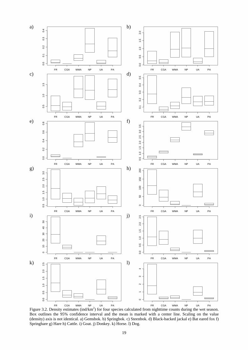
Density estimates from wet season data Density estimates based on daytime counts From the data collected during day counts in the wet season, observations sufficed for density estimates to be calculated for 11 species, whereof 5 domestic (Figure 3.1). Among the wild species, gemsbok, red hartebeest, springbok and steenbok showed significant differences in densities between protected and unprotected land use types (at the 95% confidence level), showing higher densities in the protected areas (Figure 3.1.a-d), while ground squirrel (Figure 3.1.c) and ostrich (Figure 3.1.f) did not. All domestic species (cattle, horse, donkey, goat and dog) showed significant differences in densities between protected and unprotected land use types, as seen in Figure 3.1.g-k. Density estimates based on nighttime counts From the nighttime counts in the wet season, density estimates could be calculated for 12 species, whereof 5 domestic (Figure 3.2). For the wild species for which density estimates also were possible to calculate from daytime counts (gemsbok, springbok and steenbok), the same pattern was repeated as for those estimates (Figure 3.1.acd and 3.2.abc). Among the other wild species with a predominantly higher nocturnal encounter rate, bat eared fox (Figure 3.2.e) and springhare (Figure 3.2.f) showed large differences in densities between the different land use types, whereas black-backed jackal (Figure 3.2.d) and cape/scrub (Figure 3.2.g) hare did not. The domestic species for which densities could be calculated were the same as for the daytime counts, and similarly, they all showed significant differences in densities between protected and unprotected areas (Figure 3.2.h-l). Table 3.2. Comparisons of density estimates from protected and unprotected land use types for 13 wild and 5 domestic species. Comparisons are made for each season and survey time (day/night) separately. ‘NS’ indicates that no significant difference was found and ‘-‘ that no density estimate could be calculated. Species p-values [P(DUA=DPA)] Wet season Dry season Day Night Day Night Wild

African Wild Cat - - - NS Black-backed Jackal - NS - NS Bat-eared Fox - p < 0.05 - - Cape Fox - - - NS Gemsbok p < 0.05 p < 0.05 p < 0.05 - Cape/Scrub Hare - NS - NS Ground Squirrel NS - p < 0.05 - Ostrich NS - NS - Red Hartebeest p < 0.05 - NS - Springhare - p < 0.05 - p < 0.05 Springbok p < 0.05 p < 0.05 NS - Steenbok p < 0.05 p < 0.05 p < 0.05 p < 0.05 Yellow Mongoose - - NS - Domestic Cattle p < 0.05 p < 0.05 p < 0.05 p < 0.05 Dog p < 0.05 p < 0.05 p < 0.05 - Domestic cat p < 0.05 p < 0.05 p < 0.05 - Goat p < 0.05 p < 0.05 p < 0.05 - Horse p < 0.05 p < 0.05 p < 0.05 -

a)

FR CGA WMA NP UA PA

0.0

0.2

0.4

0.6

0.8

1.0 b)

FR CGA WMA NP UA PA

01

23

4

c)

FR CGA WMA NP UA PA

0.0

0.5

1.0

1.5

2.0

2.5

d)

FR CGA WMA NP UA PA

0.5

1.0

1.5

2.0

e)

FR CGA WMA NP UA PA

0.0

0.5

1.0

1.5

2.0

2.5

3.0

f)

FR CGA WMA NP UA PA

0.05

0.10

0.15

0.20

g)

FR CGA WMA NP UA PA

020

4060

8010

0

h)

FR CGA WMA NP UA PA

02

46

810

12

i)

FR CGA WMA NP UA PA

05

1015

j)

FR CGA WMA NP UA PA

01

23

4

k)

FR CGA WMA NP UA PA

05

1015

Figure 3.1. Density estimates (ind/km2) for four species calculated from daytime counts during the wet season. Box outlines the 95% confidence interval and the mean is marked with a center line. Scaling on the value (density) axis is not identical. a) Gemsbok. b) Red Hartebeest. c) Springbok. d) Steenbok. e) Ground Squirrel. f) Ostrich. g) Cattle. h) Goat. i) Donkey. j) Horse. k) Dog.

18

a)

FR CGA WMA NP UA PA

0.0

0.1

0.2

0.3

0.4

b)

FR CGA WMA NP UA PA

0.0

0.5

1.0

1.5

2.0

c)

FR CGA WMA NP UA PA

0.5

1.0

1.5

d)

FR CGA WMA NP UA PA

0.1

0.2

0.3

0.4

0.5

e)

FR CGA WMA NP UA PA

0.0

0.2

0.4

0.6

0.8

f)

FR CGA WMA NP UA PA

0.5

1.0

1.5

2.0

2.5

3.0

3.5

g)

FR CGA WMA NP UA PA

0.5

1.0

1.5

2.0

2.5

3.0

h)

FR CGA WMA NP UA PA

050

100

150

200

i)

FR CGA WMA NP UA PA

010

2030

4050

j)

FR CGA WMA NP UA PA

0.0

0.5

1.0

1.5

2.0

2.5

k)

FR CGA WMA NP UA PA

0.0

0.5

1.0

1.5

2.0

2.5

l)

FR CGA WMA NP UA PA

01

23

4

Figure 3.2. Density estimates (ind/km2) for four species calculated from nighttime counts during the wet season. Box outlines the 95% confidence interval and the mean is marked with a center line. Scaling on the value (density) axis is not identical. a) Gemsbok. b) Springbok. c) Steenbok. d) Black-backed jackal e) Bat eared fox f) Springhare g) Hare h) Cattle. i) Goat. j) Donkey. k) Horse. l) Dog.

19

a)

FR CGA WMA NP UA PA

02

46

810

b)

FR CGA WMA NP UA PA

02

46

810

1214

c)

FR CGA WMA NP UA PA

02

46

810

d)

FR CGA WMA NP UA PA

0.5

1.0

1.5

2.0

2.5

3.0

e)

FR CGA WMA NP UA PA

05

1015

20

f)

FR CGA WMA NP UA PA

05

1015

g)

FR CGA WMA NP UA PA

0.00

0.10

0.20

0.30

h)

FR CGA WMA NP UA PA

020

4060

8010

0

i)

FR CGA WMA NP UA PA

010

2030

4050

j)

FR CGA WMA NP UA PA

02

46

810

k)

FR CGA WMA NP UA PA

01

23

4

l)

FR CGA WMA NP UA PA

01

23

4

Figure 3.3. Density estimates (ind/km2) for four species calculated from daytime counts during the dry season. Box outlines the 95% confidence interval and the mean is marked with a center line. Scaling on the value (density) axis is not identical. a) Gemsbok. b) Red hartebeest. c) Springbok. d) Steenbok. e) Ground Squirrel. f) Yellow mongoose. g) Ostrich. h) Cattle. i) Goat. j) Donkey. k) Horse. l) Dog.

20

a)

FR CGA WMA NP UA PA

0.5

1.5

2.5

3.5

b)

FR CGA WMA NP UA PA

0.0

0.5

1.0

1.5

2.0

c)

FR CGA WMA NP UA PA

0.0

0.2

0.4

0.6

0.8

1.0

d)

FR CGA WMA NP UA PA

0.2

0.4

0.6

0.8

e)

FR CGA WMA NP UA PA

1.5

2.0

2.5

3.0

3.5

4.0

4.5

f)

FR CGA WMA NP UA PA

05

1015

2025

30

g)

FR CGA WMA NP UA PA

010

2030

4050

Figure 3.4. Density estimates (ind/km2) for four species calculated from nighttime counts during the dry season. Box outlines the 95% confidence interval and the mean is marked with a center line. Scaling on the value (density) axis is not identical. a) Steenbok. b) Black-backed jackal. c) Cape fox. d) African wild cat. e) Springhare. f) Hare. g) Cattle.

21

22

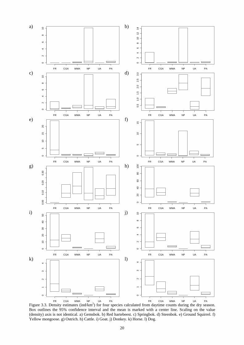
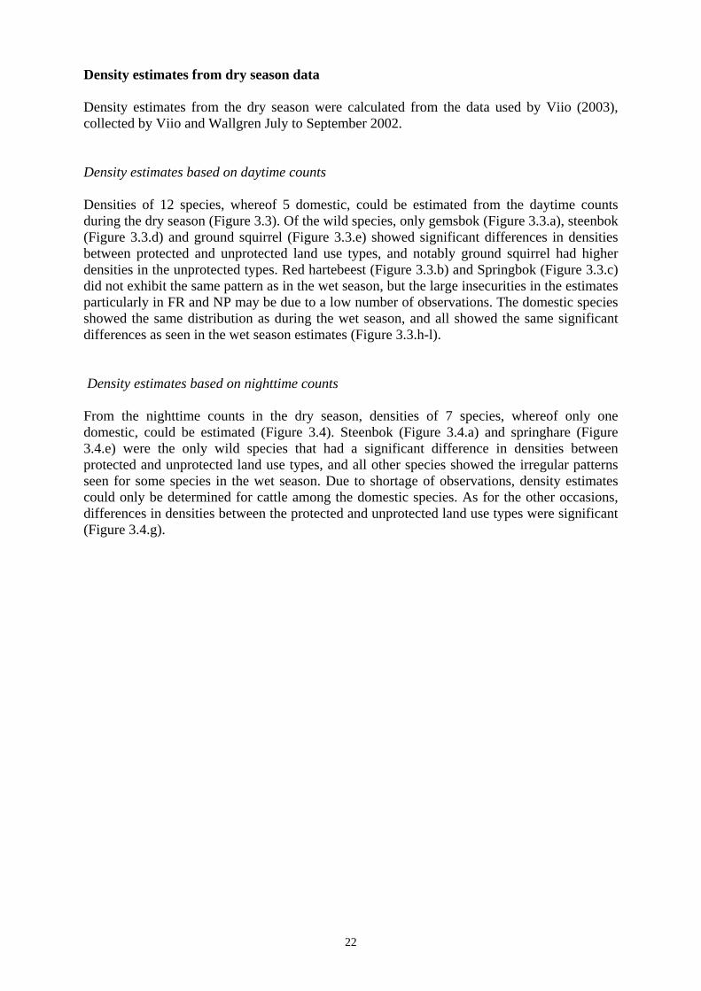
Density estimates from dry season data Density estimates from the dry season were calculated from the data used by Viio (2003), collected by Viio and Wallgren July to September 2002. Density estimates based on daytime counts Densities of 12 species, whereof 5 domestic, could be estimated from the daytime counts during the dry season (Figure 3.3). Of the wild species, only gemsbok (Figure 3.3.a), steenbok (Figure 3.3.d) and ground squirrel (Figure 3.3.e) showed significant differences in densities between protected and unprotected land use types, and notably ground squirrel had higher densities in the unprotected types. Red hartebeest (Figure 3.3.b) and Springbok (Figure 3.3.c) did not exhibit the same pattern as in the wet season, but the large insecurities in the estimates particularly in FR and NP may be due to a low number of observations. The domestic species showed the same distribution as during the wet season, and all showed the same significant differences as seen in the wet season estimates (Figure 3.3.h-l). Density estimates based on nighttime counts From the nighttime counts in the dry season, densities of 7 species, whereof only one domestic, could be estimated (Figure 3.4). Steenbok (Figure 3.4.a) and springhare (Figure 3.4.e) were the only wild species that had a significant difference in densities between protected and unprotected land use types, and all other species showed the irregular patterns seen for some species in the wet season. Due to shortage of observations, density estimates could only be determined for cattle among the domestic species. As for the other occasions, differences in densities between the protected and unprotected land use types were significant (Figure 3.4.g).

23

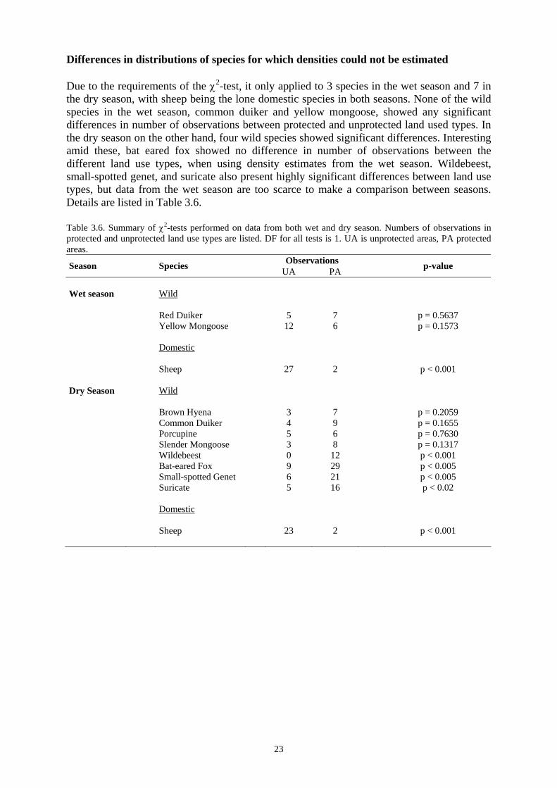
Differences in distributions of species for which densities could not be estimated Due to the requirements of the χ2-test, it only applied to 3 species in the wet season and 7 in the dry season, with sheep being the lone domestic species in both seasons. None of the wild species in the wet season, common duiker and yellow mongoose, showed any significant differences in number of observations between protected and unprotected land used types. In the dry season on the other hand, four wild species showed significant differences. Interesting amid these, bat eared fox showed no difference in number of observations between the different land use types, when using density estimates from the wet season. Wildebeest, small-spotted genet, and suricate also present highly significant differences between land use types, but data from the wet season are too scarce to make a comparison between seasons. Details are listed in Table 3.6. Table 3.6. Summary of χ2-tests performed on data from both wet and dry season. Numbers of observations in protected and unprotected land use types are listed. DF for all tests is 1. UA is unprotected areas, PA protected areas.

Observations Season Species UA PA p-value

Wet season Wild Red Duiker 5 7 p = 0.5637 Yellow Mongoose 12 6 p = 0.1573 Domestic Sheep 27 2 p < 0.001 Dry Season Wild Brown Hyena 3 7 p = 0.2059 Common Duiker 4 9 p = 0.1655 Porcupine 5 6 p = 0.7630 Slender Mongoose 3 8 p = 0.1317 Wildebeest 0 12 p < 0.001 Bat-eared Fox 9 29 p < 0.005 Small-spotted Genet 6 21 p < 0.005 Suricate 5 16 p < 0.02 Domestic Sheep 23 2 p < 0.001

24

Density comparisons between wet and dry season For the species for which densities could be estimated both in the wet and dry season, comparisons were made for all four land use types and for types grouped as protected and unprotected. Daytime counts allowed this to be done for 11 species, whereof 5 domestic (Table 3.7). The majority of all comparisons (77%) showed no significant difference between the seasons. Due to small sample sizes in the dry season nighttime counts, this comparison could be made for 5 species only, whereof cattle was the sole domestic (Table 3.8). 67% of the comparisons were not significant, and interestingly all differences shown for the wild species indicated higher densities in the dry season. Finally, cattle showed higher densities during the wet season in all three land use types where they occurs. Table 3.7. Comparisons of density estimates based on daytime counts between the wet and dry season. Differences are significant at the 95% confidence level, and indicated with ‘W’ and ‘D’ for higher density in the wet and dry season respectively. Species FR CGA WMA NP UA PA Wild Gemsbok W - - - W - Ground Squirrel - - - - - D Ostrich W - - - - - Red Hartebeest - - D - - - Springbok - - - - - D Steenbok - D - D - - Domestic Cattle - - - - - - Dog - D - - - - Donkey D D - - - - Goat W W D - W - Horse - - - - - - Table 3.8. Comparisons of density estimates based on nighttime counts between the wet and dry season. Differences are significant at the 95% confidence level, and indicated with ‘W’ and ‘D’ for higher density in the wet and dry season respectively. Species FR CGA WMA NP UA PA Wild Black-backed Jackal - D - - - -Cape/Scrub Hare - - - - - -Springhare D D D - D -Steenbok - - - - D - Domestic Cattle W W W - W -

25

5. DISCUSSION Effects of land use on mammal densities The large differences in mammal densities between the land use types seen in both wet and dry season, are shaped by relatively high densities of wild animals and low densities of domestic animals in the protected areas, and low densities of wild animals and high densities of domestic animals in the unprotected areas. This suggests that the generally observed decline in wildlife in the Kalahari (Crowe 1995; Verlinden 1997) at least partly can be ascribed to the increase in rangeland for livestock. I hypothesize that the reduced densities of wild ungulates may arise through three major mechanisms: 1) direct competition between livestock and wild herbivores over food resources, 2) long-term vegetational and/or environmental changes originating from grazing by domestic animals, or 3) direct disturbance from people, for instance in the form of legal or illegal hunting. No mechanism excludes another, and hence in reality the actuation may be a combination of more than one factor. Besides this, it is also plausible that the significance of the mechanisms may vary with season, time of the day, animal type and species. Three of the wild ungulates that were significantly less common in unprotected areas, gemsbok, red hartebeest and springbok are, together with wildebeest, well known to avoid livestock areas (Spinage 1992; Verlinden 1997; Bergström & Skarpe 1999). Wildebeest was in my study only observed in protected areas, but the data were insufficient for a density estimation with the DISTANCE method. Heavy grazing by livestock in unprotected areas is likely to deplete the palatable grasses and may often also cause an increase in the annual grasses and/or woody species (Skarpe 1986), altogether reducing the quality of the habitat to wild grazers like wildebeest and red hartebeest, and mixed feeders like springbok. Goats may correspondingly decrease the availability of good browse to wild browsers such as gemsbok. In addition to this, wildebeest used to migrate into the western parts of the Kalahari in the wet season, but this has declined throughout the 20th century (Spinage 1992). Subsequently, the erection of veterinary cordon fences rendered the species on the verge of extinction in the area, as our results bear witness of. In all probability, this scenario is also the case of the eland (Knight 1995), of which only one observation was made (in the wet season). Furthermore, Bergström & Skarpe (1999) and Wallgren et. al. (submitted) showed the existence of a gap in the distributions between domestic and wild herbivores in relation to villages, where the nearest-to-village wild herbivores were observed in general more than 10 km farther away from the villages than the farthest-to-village observation of domestic animals. This gap cannot be explained by the mechanisms of vegetational change or direct competition, and suggests that direct disturbance, probably in the form of hunting, plays an important role as a mechanism behind this scenario. Whereas the data were too scarce to allow density estimations with the DISTANCE method for the large predators – lion, leopard, cheetah, spotted hyena, not a single observation was made in the unprotected areas (in the wet season). This of course coincides well with the observed density differences between the protected and unprotected areas for the large wild herbivores discussed above. As prey becomes scanty in the unprotected areas, predators are likely to avoid these and seek subsistence elsewhere, evidently in the protected areas. This pattern was also observed by Viio (2003), and is at least qualitatively comparable with the results from aerial surveys in the Kgalagadi district by Bonifica (1992), who estimated the density of lions (the only of the large predators discussed above to be recorded in the aerial surveys) to be lower outside of protected areas than within.

26

Black-backed jackal presented similar overall densities in protected and unprotected land use types, which might be explained by its highly adaptable feeding habits. Black-backed jackals are known to prey on young goats and sheep in Southern-African ranches, which may account for this result. Moreover, upon breaking the land use types down to the four original types, a different and more variable pattern emerged. High densities occurred in the NP:s and FR, and relatively low in the WMA:s and CGA:s. Most likely, FR:s with large concentrations of prey (goats and sheep) along with high levels of bush encroachment (Skarpe 1990b) provide a good alternate habitat for the black-backed jackal, and hence these data corroborates its reputation as a highly adaptable predator. As seen in the wet season, many small mammals like slender and yellow mongoose, cape/scrub hare, porcupine, African wild cat, and cape fox revealed no differences between protected and unprotected land use types. This may elucidate another aspect of the issue on mechanisms posed earlier. If competition had been the main factor, it is likely that those species with ecological niches similar to the domestic animals introduced would be more impacted by land use, and those with different niches would be less affected. Since cattle, goats, horses and donkeys have occupied the niches of gemsboks, red hartebeests, springboks and steenboks, while mongooses, hares and foxes are unaffected, this certainly legitimates the importance of direct competition. Finally, two of the smaller species; cape/scrub hares and ground squirrels displayed no significant differences between the four land use types, even though the differences were more pronounced for the hare. Conceivably, cape/scrub hares in the unprotected land use types benefits from lower interspecific competition from for instance springhares, which although not related have comparable feeding habits (Estes 1991). Effects of seasons on mammal densities Only two of the four ungulates discussed in the previous section demonstrated the same significant differences between protected and unprotected areas in the dry season, namely gemsbok and steenbok. Yet in the case of red hartebeest and springbok, these species show large uncertainties in their estimates for Fenced Ranches and National Parks, and possibly this is the cause. Looking at it from a different point of view, red hartebeest and springbok are facultative migrates (Kok 1975 and Ritter & Bednekoff 1995, respectively), while gemsbok and steenbok are not (Estes 1991), and hence another plausible explanation to the pattern observed might well lie in actual movements. More substantial data from FR:s and NP:s in the dry season are needed to settle this matter. At a first glance, Tables 3.7 and 3.8 outlines the picture of differences between wet and dry seasons, but the situation may not be as straightforward as it seems. If one considers the wild species and the four physical land use types, 9 comparisons out of forty show significant differences, and this could well describe a general trend with regard to sheer numbers. However, upon a closer examination the image changes. Of the differences, 3 are linked to springhares, and the remaining 6 are randomly distributed over both species and land use types. The 2 occurring in Fenced Ranches are due to the fact that no gemsboks or ostriches were observed in FR:s in the dry season, and only a few observations could have omitted them. Overall, the negative evidence heaps only for one trend, which spells that differences between land use types occur, but they have in general little to do with the changing of the seasons. Finally, in the broader sense, one must bear in mind that this is only a piecemeal of the truth. The trends postulated above would surely be different, if large herds of the highly migratory wildebeest and eland had still been present.

27

Conclusions Land use evidently has an important influence on mammal densities in the southwestern Kalahari. The large herbivores clearly avoid livestock areas, which might be caused by direct competition, vegetational change and/or direct disturbance (probably hunting). In all likelihood as an effect of this, the large predators seem to follow the pattern of their prey. However, not all species are affected in the same way. Notably many smaller mammals, including carnivores, omnivores as well as herbivores, are not at all impacted by the differences in land use regimes. This may originate, in the case of the herbivores, at least partly from the fact that their ecological niches are too different from the niches of the domestic species, and hence do not impose competition. Essentially, the trends observed were not dependent on the changing of the seasons, but this might have been different if large herds of the highly migratory wildebeest and eland had not already left the scene. This study infers that policymakers on land use in the southwestern Kalahari should be aware that their decisions most certainly will influence the local fauna, and that no form of coexistence between livestock and the native wild fauna in the same area is easily at hand. Nonetheless, carefully designed policies incorporating both protected and unprotected areas, may allow an ecologically sustainable development suitable to support both the livestock and ecotourism sectors. Ideally, this would benefit the people of Botswana, along with its unique nature, in the short, as well as in the long term perspective.

28

6. ACKNOWLEDGEMENTS First of all I wish to thank Karin Carlsson, who has been with me from the beginning and all the way through, with her indefatigable energy always being a source of inspiration. Also thanks to Hudson Modise for thorough assistance with the field work, and Märtha Wallgren for teaching us all the tricks in the book about working in the bush, and for providing me with the dry season data and valuable ideas concerning data handling and processing. Thanks also to Tanja Viio and Maxwell Geean for collecting the dry season data. Thanks to Christina Skarpe for proposing this study in the first place, believing in me, and giving her indispensable support with the field work along with analyses and important suggestions to the manuscript. Thanks also to Bo Tallmark for believing in me and passing on his creative spirit, and to Nkobi Moleele for assisting us in Botswana. Thanks to Sigbjorn Stokke at the Norwegian Institute for Nature Research for his generous course on distance sampling. Thanks to the Swedish International Development Cooperation Agency (SIDA) for funding this project through ATE, The Committee of Tropical Ecology at Uppsala University, and thanks to ATE for believing in the project. Thanks to the MAPOSDA project (financed by the EU, INCO Project No. ACA4-CT-2001-10050). Thanks also to the Office of the President, Gaborone, Botswana, for providing us with the research permit, and to the Department of Wildlife and National Parks for our permission to work in the park. An explicit thanks to the rangers at Mabuasehube for all their help with our car breakdowns.

29

REFERENCES Bergström, R. & Skarpe, C. 1999. The abundance of large wild herbivores in a semi-arid savanna in relation to seasons, pans and livestock. African Journal of Ecology, Vol. 37, p. 12-26. Bonifica. 1992. Initial Measures for the Conservation of the Kalahari Ecosystem. Final Report to the Department of Wildlife and National Parks, Government of Botswana. Broekhuis, J. F . 1997. Land use planning for wildlife conservation and economic development. In: Proceedings of a national conference on conservation and management of wildlife in Botswana. Strategies for the twenty first century, p. 140-151. DWNP, Botswana. Buckland, S.T., Anderson, D.R., Burnham, K.P. and Laake, J.L. 1993. Distance Sampling: Estimating Abundance of Biological Populations. Chapman and Hall, London. Crowe, D. 1995. Status of selected wildlife resources in Botswana and recommendations for conservation actions. In: Ed. K. Leggett. Proceedings of a Symposium on the Present Status of Wildlife and its Future in Botswana. Gaborone: The Kalahari Conservation Society and The Chobe Wildlife Trust. Estes, R. D. 1991. The behaviour guide to African mammals: including hoofed mammals, carnivores, primates. University of California Press, London. Gibson, C. C. 1991. Politicians and poachers: The Political Economy of Wildlife Policy in Africa. Cambridge University Press, New York. Granlund, L. 2001. The abundance of game in relation to villages, livestock and pans – a study in southwestern Kalahari, Botswana. Committee of Tropical Ecology, Minor Field Study 73. Uppsala University. Neumann, R. P. 1997. Primitive Ideas: Protected Area Buffer Zones and the Politics of Land in Africa. Development and change, Vol. 28, No. 3, p. 559-82. Knight, M. H. 1995. Drought-related mortality of wildlife in the southern Kalahari and the role of man. African Journal of Ecology, Vol. 33, p. 377-394. Kok, O. B. 1974. Behaviour and ecology of the red hartebeest (Alcelaphus buselaphus caama). Nature Conservation, Miscellaneous publication No. 4. Orange Free State Provincial Administration, South Africa. Parris, R. 1970. Important Role of the Kalahari Pans. African Wild Life, Vol. 24, p. 234-237. Parris, R. & Child, G. 1973. The importance of pans to wildlife in the Kalahari and the effect of human settlements on these areas. Journal of Southern African Wildlife management Association, Vol.3, No. 1, p 1-8. Perkins, J. S. 1996. Botswana: Fencing out the equity issue. Cattleposts and cattle ranching in the Kalahari Desert. Journal of Arid Environments, Vol. 33, p. 503-517. Pike, J. G., 1971. Rainfall over Botswana. Botswana Notes and Records, Spec. Ed. 1, p. 69-76. R Development Core Team. 2004. R: A language and environment for statistical computing. R Foundation for Statistical Computing, Vienna, Austria. ISBN 3-900051-07-0, http://www.R-project.org. Ritter, R. C. & Bednekoff, P. A. 1995. Dry season water, female movements and male territoriality in springbok: preliminary evidence of waterhole-directed sexual selection. African Journal of Ecology, Vol. 33, p. 395-404. Skarpe, C. 1986. Plant community structure in relation to grazing and environmental changes along a north-south transect in the western Kalahari. Vegetatio, Vol. 68, p. 3-18. Skarpe, C. 1990a. Shrub layer dynamics under different herbivore densities in an arid savanna, Botswana. Journal of Applied Ecology, Vol. 27, p. 873-885. Skarpe, C. 1990b. Structure of the woody vegetation in disturbed and undisturbed arid savanna, Botswana. Vegetatio, Vol. 87, p. 11-18.

30

Skarpe, C. 2000. Desertification, no-change or alternative states: Can we trust simple models on livestock impact in dry rangelands? Applied Vegetation Science, Vol. 3, p. 261-268. Smithers, R. H. N. 1992. Land mammals of southern Africa. – a field guide. Spinage, C. A. 1992. The decline of the Kalahari wildebeest. Oryx, Vol. 26, No. 3. p. 147-150. Stuart, C. & Stuart, T. 2001. Field Guide to Mammals of Southern Africa, 3rd ed. Struik Publishers, Cape Town. Thomas, D. S. G. & Shaw, P.A. 1991. The Kalahari environment. Cambridge University Press. Cambridge. Thomas, D. S. G., Sporton, D., Perkins, J. 2000. The environmental impact of livestock ranches in the Kalahari, Botswana: Natural resource use, ecological change and human response in a dynamic dryland system. Land degradation & development, Vol. 11, p. 327-341. Thomas, L., Laake, J. L., Strindberg, S., Marques, F. F. C., Buckland, S. T., Borchers, D. L., Anderson, D. R., Burnham, K. P., Hedley, S. L., Pollard, J. H. and Bishop, J. R. B. 2003. Distance 4.1. Release 2. Research Unit for Wildlife Population Assessment, University of St. Andrews, UK. http://www.ruwpa.st-and.ac.uk/distance/ Thouless, C. R. 1998. Large mammals inside and outside protected areas in the Kalahari. Transactions of the Royal Society of South Africa. Vol. 53, No. 2, p. 245-255. du Toit, J., Walker, B. H., Campbell B. M. 2004. Conserving tropical nature: current challenges for ecologists. Trends in Ecology and Evolution, Vol. 19, No. 1, p. 12-17. Verlinden, A. 1997. Human settlements and wildlife distribution in the southern Kalahari of Botswana. Biological Conservation, Vol. 82, p. 129-136. Viio, T. 2003. Does land use affect mammal diversity in savannah ecosystems? Committee of Tropical Ecology, Minor Field Study 89. Uppsala University. Wackerly, D. D., Mendenhall III, W., Schaeffer, R. L. 2002. Mathematical statistics with applications. Duxbury, California. Wallgren, M. S. 2001. Mammal communities in the southern Kalahari – distribution and species composition. M.Sc. Thesis. Committee of Tropical Ecology, Minor Field Study 69. Uppsala University. Wallgren, M., Skarpe, C., Bergström, R., Danell, K. & Granlund, L. Functional structure of mammal communities in relation to human disturbance and key resources in southern Africa (submitted manuscript). Wildlife Conservation Policy. 1986. Government Paper No. 1. Government Printer, Gaborone.