Embed Size (px)
Citation preview

INFLUENCE OF BINDER LOSS MODULUS ON THE FATIGUE PERFORMANCEOF ASPHALT CONCRETE PAVEMENTS
by
J.A. Deacon, J.T. Harvey, A. Tayebali, and C.L. Monismith,
Paper offered for consideration at the 1997 Annual Meeting of the Associationof Asphalt Paving Technologists
Introduction
The asphalt binder specifications resulting from the Strategic Highway Research Program
(SHRP) Asphalt Research Program are performance-based and attempt to address the major
distress modes encountered in asphalt concrete pavements: fatigue cracking, rutting, and low-
temperature cracking. The binder parameters are: 1) for rutting - G*/sin6 measured on the
original binder at the maximum pavement temperaturel; 2) for low temperature cracking -
creep stiffness and the m-value2 measured on the residue from the PAV test at the minimum
pavement temperature1 plus 1OC; and 3) for fatigue - G*sinG measured on the PAV aged
residue at an intermediate pavement temperature3 (1-2).
The use of the parameter GTsinG to control fatigue cracking was based in part on the
results of controlled-strain fatigue tests on mixes containing two MRL aggregates and eight
MRL asphalts developed as a part of the SHRP research effort (3). The results of these mix
studies indicated that mix fatigue life was a function of the mix parameter S,sin& the initial
mix loss stiffness in sinusoidal loading. Thus it seemed logical to use the binder loss
stiffness as the parameter to control mix fatigue since fatigue is attributable to cracking in the
binder phase of the mix. Very limited data developed from tests on asphalts used in the
Zaca-Wigmore Test Road suggested that a maximum value of 5 MPa
1Pavement temperatures are determined from temperature datapavement site using algorithms contained in the Superpave software.
for this parameter
representative of the
T h ee m-value is a measure of the slope of the log stiffness versus log timerelationship.
3The intermediate temperature is approximately the average of the maximum andminimum pavement design temperature.
appeared appropriate (I). Justification for an upper limit on this parameter was also included
in Reference 4 in which it was argued that fatigue cracking could be exacerbated during
spring thaw in temperate regions of the U.S. when the subgrade is weak and the asphalt-
bound layer is relatively stiff.
While the m-value parameter, as noted above, is primarily associated with the control
of low temperature cracking, presumably the specification limit on this parameter is also used
to control fatigue cracking (I). It was argued that the m-value provides control of the slope
of the creep compliance curve which, in turn, is related to the spectrum of relaxation times
of the binder. Since the slope of the mix creep curve is controlled to a certain extent by the
binder and since this slope has been related to fatigue cracking as well as thermal cracking
(5), the argument was advanced that controlling the m-value might assist in the control of
fatigue cracking.
Results from fatigue tests on neat asphalt binders presented by Heukelom (6) indicated
that their fatigue response is dependent on the ratio of the elastic modulus to the modulus of
delayed elasticity. The elastic modulus, EasP, corresponds to the value of stiffness at short
loading times, i.e., Sasp = EasP as t -+ 0.
In turn, Heukelom defined the delayed elastic modulus, Dasp, as follows:
1 1 1- --D
rnPS
rnPE
rnP(1)
He further related this parameter to the delayed-elastic energy per loading in fatigue, Qd fat,9
and developed the following expression relating Qd fat9 to the energy consumed by the delayed
elastic deformation during a bending test, Qd bending:9

Qd&t = S@P C
Qd bending Easp-s, l fl
in which C = experimentally determined coefficient equal to
stress mode of loading and about 50 for controlled-strain and
in fatigue.
3
(2)
about 40 for the controlled-
N = number of load repetitions
Although the Heukelom results would thus seem to reinforce the decision to use
G*sind parameter as a specification parameter, unfortunately it is not sufficient to control
fatigue response in a pavement structure by simply controlling binder characteristics. Other
factors including mix properties, pavement thickness, traffic loading, and the temperature
environment are also critically important determinants of fatigue performance. This was
stated in Reference 3 where it was shown that the binder loss stiffness did not correlate well
with pavement performance.
It is the purpose of this paper to briefly summarize the results of the limited test
program incorporated in Reference 3 which examined effects of binder loss stiffness on
performance together with a more detailed study of the effects of binder loss stiffness on the
simulated fatigue performance of 18 different pavement sections designed according to
Caltrans procedures (II) and used in three different temperature environments in California.
The results of these studies indicate that the current specification parameter to control
fatigue cracking is likely to be counterproductive for sections of asphalt concrete more than
about 50 mm (2 in.) in thickness and suggests an alternative approach to assure adequate
fatigue resistance in situ.

Asphalt Binder Effects on Laboratorv Mix Performance
In the investigation reported in Reference 3, controlled-strain fatigue tests were performed on
32 different mixes (containing eight MRL asphalts, two MRL aggregates, and two air-void
contents). The test program was referred to as the 8 x 2 experiment. The fatigue tests,
performed on specimens 50 mm (2 in.) high, 63.5 mm (2.5 in.) wide, and 38 mm (15 in.)
long were conducted at a frequency of 10 Hz and at 20C.
Measurements of G” (G*sinQ at 20C (68F) and 10 Hz frequency for thin film oven
test (TFOT)-aged asphalt binders were provided by SHRP Project A-002A. Mix fatigue
testing was conducted at the same temperature and loading frequency. Table 1 presents the
asphalt binder properties measured by dynamic mechanical analysis (DMA). Relationships
were evaluated between asphalt binder properties and
l laboratory-determined fatigue life of asphalt-aggregate mixes under third-point
controlled-strain flexural beam fatigue testing, and
l in situ fatigue life of asphalt-aggregate mixes predicted by linear elastic layer
analysis in which the maximum tensile strain was calculated in simulated
pavements.
Binder Effects on Laboratorv Mix Performance. Regression analysis was used to relate the
asphalt binder loss stiffness (G*sinG) to the laboratory fatigue life of mixes at 20C (68F) and
10 Hz frequency. Table 2 shows the coefficients of determination (R2) for the laboratory
fatigue life versus binder loss stiffness and binder complex stiffness regressions, stratified by
aggregate source and air-void content at the 400 microstrain level. For a given aggregate

and air-void content, mix fatigue life (In cycles to failure) correlated quite well with loss
stiffness of the aged asphalt binder (Figures 1 and 2). Increases in binder r loss stiffness were
accompanied by rather significant decreases in mix fatigue resistance. Aggregate type and
air-void content were also important: RH aggregates generally produced more fatigue-
resistant mixes than did RD aggregates, and mixes with low air-void contents generally
proved superior to those with high air-void contents, The loss stiffness of the aged binder
was a slightly better predictor variable than the. complex stiffness (Table 2).
Coefficients of determination from additional regressions on adjusted fatigue life
(fatigue life adjusted to 4-percent and 7-percent air-void contents) versus the binder loss
stiffness are summarized below:
Effect
Aggregate source (across air-void contents,strain level, replicates)
Air-void contents (across aggregate source,strain level, and replicates)
Strain level (micro in. /in.) (across aggregatesource, air-void contents, and replicates)
Level
RHRD
4 %7 %
400700
Coefficient of DeterminationFatigue Life Versus G*sinS
0.970.64
0.680.95
0.810.94
Binder Effects on In-Situ Mix Performance. In-situ mix performance was simulated by
linear elastic layer analysis (ELSYM) of the response of three typical pavement structures
to a 44.4 kN (10,000 lb) wheel load (305 mm [12 in.] center-to-center dual tires with 690
kPa [ 100 psi] contact pressure). The first two structures were three-layered systems which
consisted of 10.2 and 15.2 cm (4 and 6 in.) asphalt-aggregate surfaces with layer stiffnesses
determined from laboratory flexural fatigue testing for each of the 32 asphalt-aggregate mixes
b

6
(eight asphalts x two aggregates x two air-void contents) and an assumed Poisson’s ratio of
0.35. The base thicknesses were 40.6 and 30.5 cm (16 and 12 in.) for the 10.2 and 15.2 cm
(4 and 6 in.) thick asphalt layers, respectively: the base modulus was 138 MPa (20,000 psi)
and its Poisson’s ratio, 0.3. The subgrade had a modulus of 69 MPa (10,000 psi) and a
Poisson’s ratio of 0.3. The third pavement was a two-layer structure with a 25.4 cm (10 in.)
asphalt-aggregate surface placed directly on a weak subgrade having a modulus of 34.5 MPa
(5,000 psi) and Poisson’s ratio of 0.4.
For each pavement structure, the maximum tensile strain at the bottom of the asphalt
layer was determined from elastic analysis for the 32 asphalt-aggregate mixes (a total of 96
ELSYM simulations for the three pavement sections under consideration).
For each of the 32 asphalt-aggregate mixes, laboratory fatigue life versus tensile
strain regression models of the following form were determined:
Iv-- = K, (l/E>K’ (3)
in which N, = laboratory fatigue life, E = tensile strain, and K1, and K2, = experimentally
determined regression coefficients.
By using the tensile strain at the bottom of the asphalt-aggregate layer as determined
from the elastic pavement analysis and the laboratory fatigue relationships between the tensile
strain and fatigue life, cycles to failure in the simulated pavement structures for the 32
asphalt-aggregate mixes were determined. The cycles to failure for the simulated structures
were then correlated to binder loss stiffnesses.
The analysis indicated that simulated pavement performance was not well correlated
with binder loss stiffness (Table 3) with or without stratification by aggregate type and air-

void content. Typical relationships between the binder loss stiffness and simulated field
cycles to failure for the three-layered structure with a 15.2 cm (6 in.) asphalt-aggregate layer
are presented in Figures 3 and 4. It is interesting that the effects of binder loss stiffness and
aggregate type on fatigue resistance were different depending on which of the two measures
of fatigue response was used. Using laboratory fatigue life (natural logarithmic function of
cycles to failure at 400 microstrain), a superior response was associated with smaller binder
loss stiffness and the RH aggregate (Figures 1 and 2). Using field simulations of cycles to
failure, a superior response was associated with larger binder loss stiffness and the RD
aggregate (Figures 3 and 4). Lower air-void contents generally were advantageous for both
laboratory and simulated fatigue lives.
Accuracy of the regressions was found to improve slightly with an increase in asphalt
layer thickness (Table 3), but all trends were similar for the three pavement structures.
These findings underscore the importance of using mechanistic analyses to properly interpret
laboratory fatigue data.
Summarv of the Asphalt Binder Effects on Mix Performance. The results of this
investigation of the effect of asphalt binder loss stiffness on laboratory and field-simulated
asphalt-aggregate mix fatigue performance can be summarized as follows:
l The laboratory fatigue resistance of asphalt-aggregate mixes is sensitive to the
type of asphalt binder. The loss stiffness of the aged binder provides a good
indication of the relative laboratory fatigue resistance of otherwise identical
mixes. Accordingly, the binder loss stiffness seems, at first glance, to be an
attractive candidate for inclusion in binder specifications.

8
l The loss stiffness of the binder, however, is generally not a sufficient indicator
of the relative fatigue resistance of asphalt-aggregate mixes. Other mix
characteristics, such as aggregate type and air-void content, also significantly
contribute to laboratory fatigue resistance. Accordingly, a binder specification
alone is insufficient to ensure satisfactory fatigue performance of pavements in
situ.
Having laboratory test data on mixes is a necessary condition for
characterizing fatigue behavior. However, laboratory testing must be
supplemented by mechanistic analyses to determine how mixes are likely to
perform in the pavement structure under anticipated traffic loads and
environmental conditions. Accordingly, mix specifications must address
composite effects of mix properties, pavement structure, traffic loading, and
environment on pavement performance.
Binder Effects on Fatigue Response of Asphalt Concrete Mixes in Pavements Designed
According to Caltrans Procedures
Reference 7 includes a mix design and analysis system which explicitly accounts for fatigue
distress. This system relies on laboratory flexural-fatigue testing for mix evaluation and
incorporates an analysis system for properly interpreting test results. It recognizes that mix
performance in situ depends on critical interactions between mix properties and in-situ
conditions, thus providing not only sensitivity to mix behavior but also sensitivity to the in-
situ traffic, climatic, and structural environments as well.

System Description. As presented herein, the fatigue design and analysis system assumes
that a trial mix has been selected, and it evaluates the likelihood that this mix will
satisfactorily resist fatigue cracking in the design pavement under anticipated traffic and
temperature conditions.
In essence, a mix is expected to perform satisfactorily if the number of load
repetitions sustainable in laboratory testing exceeds the number of load repetitions anticipated
in service. To minimize laboratory costs, testing is at an accelerated rate and, for normal
asphalts, at a single temperature. Using the SHRP developed controlled-strain, flexural-
fatigue apparatus (3), testing can usually be accomplished within a 24- to 48-hour period.
The strain at which the number of laboratory repetitions must be estimated is computed using
multilayer elastic theory. For this computation, the strain of interest is the maximum
principal tensile strain at the bottom of the asphalt-bound layer in the design pavement. A
40 kN (9,000-pound), dual-tire load is applied, and the mix stiffness corresponds to the
laboratory test temperature.
Traffic is represented by the number of equivalent single axle loads (ESALs) in the
critical or design lane during the design period. Because these ESALs accumulate within a
mixed temperature environment, it is necessary to apply a factor, herein termed the
temperature conversion factor (TCF), to convert design ESALs to their equivalent at a
single temperature, that used in the laboratory testing. Experience has shown that it is also
necessary to apply a shift factor (SF), accounting for a host of factors such as traffic wander,
crack propagation rate, construction variability, different frequencies of loading, etc., to
assure that load repetitions in the field are commensurate with those in the laboratory.
Because of uncertainty or variability in all of the measurements, simulations, and

10
predictions, there is some risk that a mix will fail in service even if its laboratory resistance
is determined, by the aforedescribed process, to exceed the design loading. Fortunately the
risk of failure can be limited to a tolerable level by applying a reliability multiplier to the
design loading before comparisons are made with the laboratory resistance. The fatigue
design and analysis system incorporates risk assessments in this way.
In summary a mix is deemed to be suitable for use in the selected pavement structure
to mitigate fatigue cracking when:
N > ESALs T C F 4 4 SF (4)
in which N = the number of laboratory load repetitions to failure under the anticipated in-
situ strain level, ESALs = the number of equivalent, 80 kN (18,000-pound) single axle loads
expected in the design lane during the design period, TCF = the temperature conversion
factor, M = the reliability multiplier, and SF = the shift factor. When a mix under
consideration doesn’t meet this requirement, the designer has a wide range of options
including adjusting the mix by adding more asphalt and/or reducing the air voids, using a
different asphalt or aggregate, increasing the pavement thickness, and even allowing an
increased risk of premature failure,
Pavement Structures. To examine the effects of binder loss modulus on simulated field
performance, 18 pavement structures were designed following Caltrans procedures for the
following conditions; three levels of traffic index (7, 11, and 15), three levels of subgrade
R-value (5, 20, and 40), and two base types (Class B cement treated base and Class 2

11
aggregate base) .4
The traffic index (TI) is used in the Caltrans design method as a measure of the
number of equivalent single axle loads (ESALs) expected in the design period. The range in
ESALs corresponding to traffic indices of 7, 11, and 15 are 89,800 to 164,000, 4,500,000
to 6,600,000, and 64,300,000 to 84,700,000, respectively. The selected TI levels span the
range of low, medium, and very high traffic loadings on state highway pavements.
The three subgrade R-values of 5, 20, and 40 span a similarly wide range in subgrade
strength and load resistance. Elastic moduli were estimated to be 26.5, 84.1 and 161.3 MPa
(3,850, 12,200, and 23,400 psi) for R-values of 5, 20, and 40, respectively (8).
Base materials included Class B cement treated base and Class 2 aggregate base. The
Type II cement used in the Caltrans cement treated base acts principally to improve the
engineering properties of those aggregate base materials which contain a large percentage of
fines. Its percentage, limited to 2.5 percent by weight of aggregate, is insufficient to provide
strong bonding with the aggregate particles. Class 2 aggregate base is commonly used in
Caltrans pavement sections. Elastic moduli for base materials were estimated based on past
experience of the authors as follows:
Asphalt concrete thickness Class B cement treated base Class 2 aggregate base
91 to 183 mm (3.6 to 7.2 in) 276 MPa (40,000 psi) 207 MPa (30,000 psi)
198 to 305 mm (7.8 to 12.0 in) 220 MPa (32,000 psi) 172 MPa (25,000 psi)
305 to 396 mm (12.0 to 15.6 in) 172 MPa (25,000 psi) 138 MPa (20,000 psi)
Layer thicknesses were designed by conventional Caltrans practice using the
4Pavement structural sections did not include drainage layers (as is current Caltranspractice) in order to simplify the computations.

12
microcomputer program NEWCON90 to perform al l calculations . Class 2 aggregate subbase
(minimum R-value of 50) was selected for all pavements for which a subbase was included.
The minimum thickness for all base layers was 150 mm (6 in). NEWCON90’ s default
minimum thickness for aggregate subbase layers is 105 mm (4.2 in).
The default unit costs for materials in NEWCON90 were used to rank the alternative
thickness designs, and the lowest cost design was selected for each case .If several thickness
designs had the same lowest cost, the design with the thickest asphalt concrete layer was
selected.
When the subgrade R-value was 40 and NEWCON90 designs included the minimum
subbase thickness, the design was recalculated with the subbase eliminated. The rationale for
this change was that the subgrade was of nearly equal strength as the eliminated subbase, and
the added complications of constructing a very thin subbase layer would not be warrante d in
practice.
Table 4 identifies the 18 hypothetical pavements including the parameters used in
ELSYM5’s multilayered elastic analysis.
Temperature Conversion Factors. The fatigue design and analysis system has been calibrated
to conform principally with California design practice .Details are presented in this and
immediately following sections.
Temperature conversion factors were determined for three California locations,
representing a variety of climatic conditions, according to the procedure described in
Reference 9. The locations included: Blue Canyon in Placer County (mountain), Daggett
Airport in San Bernadino County (desert), and Santa Barbara Airport in Santa Barbara

County (coastal). At each location, two hypothetical
mm (4.0 in.) and 203 mm (8.0 in.) surface courses.
pavements were
The asphalt mix
13
examined having 102
was thought to be
representative of those used in California, and laboratory stiffnesses and fatigue lives were
measured and characterized during the recent SHRP A-003A investigation. Pavement
temperature profiles were simulated using the climatic-materials-structural (CMS) pavement
analysis model originally developed at the University of Illinois (10) and revised slightly to
better accommodate input/output requirements and to replace the method for computing
extraterrestrial radiation with a more suitable one.
Pavement temperature simulations spanned 10-year periods for Santa Barbara and
Daggett Airports and a 6-year period for Blue Canyon. Table 5 presents relevant location
information and climatic summaries for the three sites.7 Important parameters,used in the
temperature simulations are summarized in Table 6. The simulations produced detailed,
long-term temperature profiles for each of the two hypothetical pavements mentioned above.
Because the laboratory testing of this study was conducted at 19C, it was necessary to
compute TCFs for this temperature. Also determined were the critical temperature (the
temperature integer at the mid-point of a 5C [9F] temperature range within which the largest
amount of damage accumulates) and TCFs to the critical temperature. Results of these
computations, summarized in Table 7, confirm prior findings that TCFs are both site- as well
as pavement structure-specific. They also confirm prior findings that critical temperatures
are larger for 203 mm (8.0 in.) pavements than for 102 mm (4.0 in.) pavements and, for
both thicknesses, are considerably in excess of the test temperature of 19C. Testing at
7Necessary weather information for the three sites was obtained from NationalClimate Data Center databases.
14
critical-temperature levels would be advantageous because possible errors due to temperature-
sensitivity abnormalities and due to necessary extrapolations would be reduced. Nevertheless
the convenience of testing at cooler temperatures and uncertainties about the legitimacy of
laboratory fatigue measurements at higher temperatures dictated the choice of test
temperatures at or near to 20C.
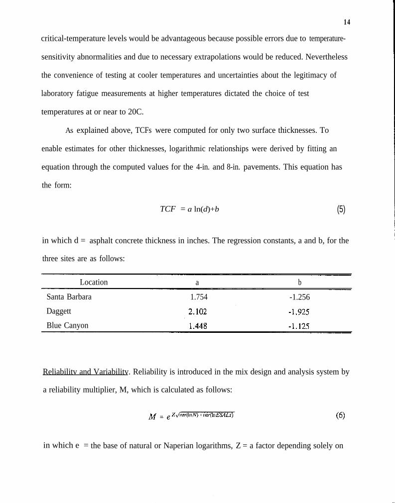
As explained above, TCFs were computed for only two surface thicknesses. To
enable estimates for other thicknesses, logarithmic relationships were derived by fitting an
equation through the computed values for the 4-in. and 8-in. pavements. This equation has
the form:
TCF = a ln(d)+b (5)
in which d = asphalt concrete thickness in inches. The regression constants, a and b, for the
three sites are as follows:
Location a b
Santa Barbara 1.754 -1.256
Daggett
Blue Canyon
Reliabilitv and Variabilitv. Reliability is introduced in the mix design and analysis system by
a reliability multiplier, M, which is calculated as follows:
in which e = the base of natural or Naperian logarithms, Z = a factor depending solely on

15
the design reliability, Var(ln N) = the variance of the logarithm of the laboratory fatigue life
estimated at the in-situ strain level under the standard, 40 kN (9,000-pound) wheel load, and
Var(ln ESALs) = the variance of the estimate of the logarithm of the design ESALs.
In this study a 95-percent reliability level has been used which corresponds to a value
for Z= 1.64. Var(ln ESALs) has been assumed to be 0.300 in the absence of better
information. Var(ln N) reflects a combination of factors including the inherent variability in
fatigue measurements (associated both with specimen preparation as well as testing equipment
and procedures), the nature of the laboratory testing program, and the extent of extrapolation
necessary for estimating fatigue life (using a least-squares, best-fit line) at the design strain
level. It is calculated as follows:
var(lnN> =s2 ( l+L+ (X -x>2I2 4x (“p-92 1 /(7)i
in which s2 = the variance in logarithm of laboratory fatigue-life measurements, n =
number of test specimens, X = ln(in-situ strain) at which In(N) must be predicted, g =
average ln(test strain), q = number of replicate specimens at each test strain level, and x P =
ln(test strain) at the pth test strain level.
Based on the study reported in Reference 11, an s2 value of 0.220 has been used. It
should be noted that the sample variance obtained in the SHRP A-003A expanded tested
program, using the same testing equipment and procedures, was 0.152. Because of greater
replication in the study reported in Reference 11, (three versus two in A-003A) and smaller
strain levels (150 and 300 microstrain versus 400 and 700 microstrain in A-003A), 0.220
seems to be the best possible estimate of s2 at the current time.

16
Shift Factor. In Reference 7 shift factors ranging from 10 to 14 were recommended for use
with the controlled-strain fatigue test methodology which had been developed, the magnitude
of the factor depending on the amount of surface cracking considered to be tolerable. For
this investigation shift factors were developed from results of laboratory fatigue and stiffness
testing of ,a representative California mix combined with the 18 different pavement structures
described above.
A mix containing 5-percent asphalt and 8-percent air voids was selected as that typical
of mixes for which the California thickness design procedure is most applicable. The
performance of this mixture in the 18 hypothetical pavement structures, representing three
traffic levels, two base types, and three subgrades, was simulated. Such simulations
produced estimates of the laboratory fatigue life (N), and the traffic index determined the in-
situ traffic loading (ESALs). The shift factor was then calculated as follows:
SF= ESALs . TCF . M
N (8)
Shift factors were thus determined for each of the 18 hypothetical pavements, In the
process, ESALs were estimated from the traffic index by the following approximate
relationship: 8
ESALs = 1.2895 . 1O-2 TI 8*2919 (9tI
TCFs were computed based on depth of the asphalt concrete layer, and separate computations
were performed for the three locations, Santa Barbara, Daggett, and Blue Canyon. To
8This equation was obtained from the expression: TI= 1.690 ESALs0.1206 which wasdeveloped by regression from the values relating TI and ESALs in the Caltrans HighwayDesign Manual (13).

17
compute the reliability multiplier (M), a 90-percent reliability was assumed, and var(ln N)
was based on an s2 of 0.220. The fatigue life (N) was computed from in-situ strain
simulations under a 40 kN (9,000-pound) dual-tire loading., Results of these computations showed a dependence of the shift-factor on both
level and traffic index: the influence of site location appeared to be relatively minor.
strain
A real
difficulty in this analysis is the fact that each of the 18 pavements does not resist fatigue
distress equally well. California design relationships do not explicitly treat fatigue distress,
and, while it is possible that most designs are at least marginally adequate, some almost
certainly are overconservative. Design to accommodate the median condition was considered
reasonable in developing a relatively conservative, first-order approximation of shift factors
that would be suitable for initial use.
It seemed logical to relate the design shift factor (the number of in-situ load
repetitions equivalent to each load application in the laboratory) to the level of pavement
strain. The rate of crack propagation, a principal difference between in-situ and laboratory.
behavior, is affected by strain level: small strains not only increase the number of load
repetitions to crack initiation but also slow the rate of crack propagation as well. The
opposite is expected for large strains.
Figure 5 shows the relationship between the 50th.percentile shift factor and the 50th-
percentile pavement microstrain. Each point represents one of the three levels of traffic
index: the power relationship has been utilized herein because it best represents the available
data. It is expressed as follows:
Design shift factor = 2.7639 l lo-’ ~~~~~~~~ for E > 0.000040 (10)

18
in which E = simulated strain in mm/mm produced by standard wheel load at the underside
o f the asphalt-concrete layer.
Influence of Binder Loss Modulus on Pavement Fatigue Performance. To analyze the effects
of binder loss modulus on pavement fatigue performance, data shown in Table 8 were
utilized. In order to perform the type of analysis necessary to demonstrate the pavement-
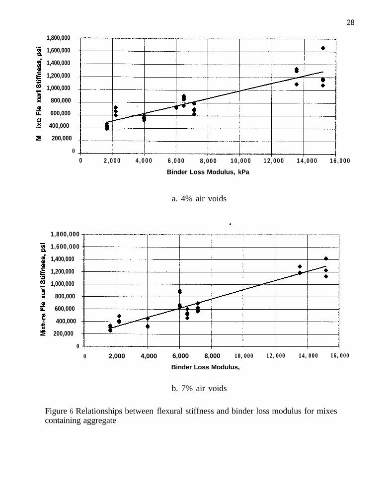
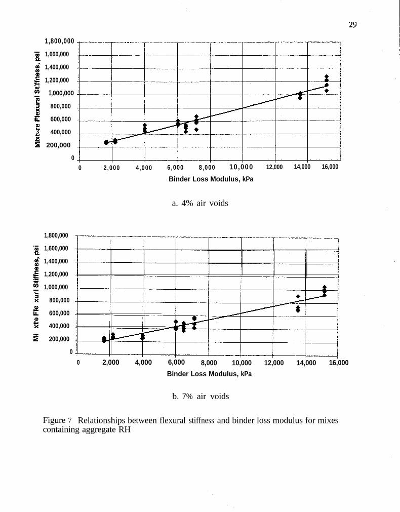
performance effects of binder loss modulus, regression relationships between laboratory
flexural stiffness and binder loss modulus and between laboratory fatigue life and binder loss
modulus were developed. Independent regressions were calibrated for four combinations of
aggregate source and air-void content, i.e., mixes with aggregates RD and RH which were
compacted to two different air-void contents. The resulting stiffness relationships are shown
in Figures 6 and 7 while the fatigue relationships are shown in Figures 8 and 9. Table 9
contains a summary of the adjusted R2 for the regressions shown in these figures.
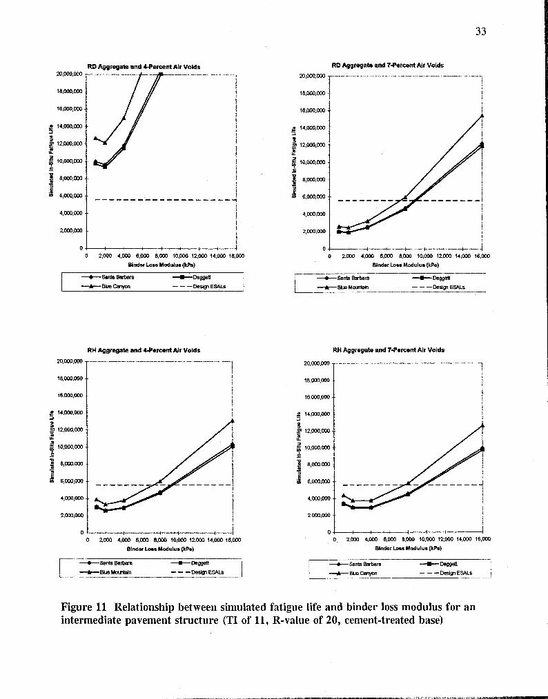
Behavior of the four mixes was simulated in the 18 pavement structures (Table 4).
The assumed load was a 40 kN (9,000 lb) dual-tire load with a 760 kPa (110 psi) contact
pressure and 335 mm (13.2 in.) center-to-center spacing. A total of 360 simulations were
performed with a 95-percent reliability level used for the analyses.
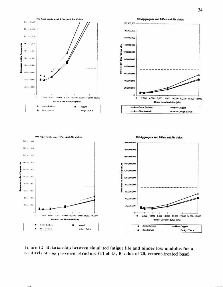
Representative results of some of the analyses are summarized in Figures 10 through
12. In essence these figures illustrate that increases in binder loss modulus above about
2,000 kPa result in increases in fatigue life. On average for the 18 hypothetical structures,, a
4,000 kPa binder increases the fatigue life above that of a 2,000 kPa binder by a factor of

19
about 1.23. Corresponding factors for 8,000 and 16,000 kPa binders are 2.14 and 4.69,
respectively.
For the pavement sections shown in Table 4, it will be noted that the thicknesses of
the asphalt-bound layers varied from about 9 1 mm (3 l 6 in.) to 4 11 mm (16.2 in.). For these
thicknesses, increases in binder loss modulus above 2,000 kPa result in increases in fatigue
life as noted above.
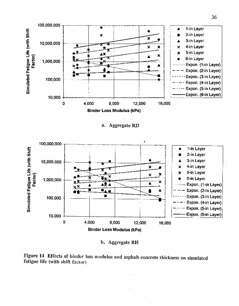
To ascertain at what pavement thickness the current binder loss criterion of the SHRP
binder specification might be appropriate, a series of simulations were performed for mixes
containing the eight asphalts and two aggregates used in the other simulations. In this
exercise only one air void content, 5.5 percent, was used for a series of pavements with
asphalt concrete thicknesses ranging from 25 mm (1.0 in,) to 152 mm (6.0 in.).
The results of these analyses are shown in Figures 13 and 14. Figure 13 illustrates
that a small loss modulus is desirable for thin asphalt concrete layers while a large loss
modulus is desirable for thicker layers. Figure 14 is similar to Figure 13 except that the
laboratory-to-field shift factor has been applied in the simulations. Because the shift factor is
larger for thicker pavements (smaller strains in Equation l0), the pattern is slightly different.
That is, except for very thin pavements, a large loss modulus always improves fatigue life.
The results of these analyses reinforce the conclusions contained in Reference 3,
particularly that the loss stiffness of the binder is not a sufficient indicator, by itself, of the
fatigue performance of asphalt concrete in actual pavement structures. Moreover, they
highlight the basic conflict between the current specification which sets a maximum limit on
loss modulus and field performance simulations which suggest that a minimum limit might be
more appropriate. The next section addresses an alternative which is recommended to the

20
current requirement for fatigue in the SHRP binder specification.
Recommended Alternative to SHRP PG Binder Specification
In the opinion of the authors, the current requirement in the SHRP binder specification to
control fatigue is inappropriate. While the parameter G*sinG of the binder is related to
laboratory fatigue response of mixes in the controlled-strain mode of loading (Figures 1 and
2) and small values do appear to be related to improved in-situ fatigue performance in thin
(50 mm [2 in.] or less) asphalt-bound layers (Figures 13 and 14), such small thicknesses are
not representative of today’s practice for asphalt layers in new or rehabilitated pavements.
G*sinG does little to assure satisfactory fatigue performance and appears to be
counterproductive for many typical pavements. Accordingly, our recommendation is to
eliminate this fatigue requirement from the current binder specification.
Such a recommendation would retain control of binder characteristics at high and low
temperatures as is currently the case (2). The low temperature requirements are, we believe,
the soundest set of parameters in the specification since they are supported by extensive
validation on mixes containing a range in conventional binders evaluated in the Thermal
Stress Restrained Specimen Test (TSRST) (12).
As a part of the low temperature requirements, a limit is set for the m-value of the
binder. It is likely that this parameter may also help to control the fatigue response of the
binder-as noted in References 1 and 5. That is, the m-value controls the slope of the creep
compliance curve which, in turn, is related to the spectrum of relaxation times of the binder.
Since presumably the slope of the creep curve is related to fatigue cracking as well as

21
thermal cracking (5) and since the
controlling the m-value the binder
slope is dependent to a certain extent on the binder, by
specification is likely, in fact, to include some control on
the fatigue characteristics of the binder.
For mixes containing other than conventional dense-graded aggregates (e.g., stone
mastic, gap graded, and large stone mixes) and/or modified binders, the mix-analysis
procedure described earlier should be followed. If modified binders are to be evaluated,
analysis should be expanded and fatigue tests should be performed at two and preferably
three temperatures. Based on experience with fatigue damage estimates in pavements
the
containing conventional mixes (dense-graded aggregates and unmodified asphalts), fatigue
testing should be performed in the range 10 to 30C (e.g., lOC, 2OC, and 30C if three
temperatures are utilized). It is also recommended that at least six specimens be tested at
each temperature, three at each of two strain levels.
Multilayer elastic analysis is recommended to estimate the principal strains occurring
on the underside of the binder-aggregate mix for the traffic expected and for the pavement
temperature range determined according to the procedure described in Reference 11.
Appropriate material moduli must be available for the various layers. Use of the linear
summation of cycle ratios cumulative damage hypothesis is suitable to accumulate damage
over the range of temperatures noted above.
This procedure will permit the selection of an adequate thickness of mix to withstand
the expected traffic in the specific environment and pavement structure in which the mix is to
be used. An economic analysis will then determine the suitability of the mix for the specific
application l
It is important to emphasize, as stated earlier, that the binder alone can not control

22
fatigue response in the pavement structure, Mix characteristics as well as the pavement
structure itself and the environment within which it is located have a significant role in
determining pavement performance.
References
1 . Anderson, D.A. and T.W. Kennedy,
Journal of the Association of Asphalt Paving
2 . AASHTO, Standard SpeciJication for
“Development of SHRP Binder Specification”,
Technologists, Vol. 62, 1993, pp. 481-507.
Performance Graded Asphalt Binder, AASHTO
Designation: MPl-93 Edition lA, September 1993; AASHTO Provisional Standards, March
1995 Edition, Washington, D.C.
3 . Tayebali, A. A., J.A. Deacon, J.S. Coplantz, F.N. Finn, and C.L. Monismith, “Part
II: Extended Test Program”, Fatigue Response of Asphalt-Aggregate Mixes, SHRP-A-404,
Strategic Highway Research Program, National Research Council, Washington, D. C., 1994.
4 . Christensen, D.W. Jr and D.A. Anderson, “Interpretation of Dynamic Mechanical
Test Data for Paving Grade Asphalt Cements”, Journal of the Association of Asphalt Paving
Technologists, Vol. 61, 1992, pp. 67-116.
5 . Lytton, R. G., J. Uzan, E.G. Fernando, R. Rogue, D. Hiltunen and S .M. Stoffels,
Development and Validation of Performance Prediction Models and Specifications for Asphalt
Binders and Paving Mixes, SHRP-A-404, Strategic Highway Research Program, National
Research Council, Washington, D.C., 1993.

6 . Heukelom, W., “Observations on. the Rheology and Fracture of Bitumens and Asphalt
Mixes”, Proceedings, Journal of the Association of Asphalt Paving Technologists, Vol. 35,
1966, pp. 358-399.
7 . Deacon, J.A., A.A. Tayebali, J.S. Coplantz, F.N. Finn, and C.L. Monismith, “Part
III: Mix Design and Analysis”, Fatigue Response of Asphalt-Aggregate Mixes, SHRP-A-404,
Strategic Highway Research Program, National Research Council, Washington, D.C., 1994.
8 . Kallas, B.F. and J.F. Shook, San Diego County Experimental Base Project-Final
Report, Research Report 77-1 (RR-77-l), The Asphalt Institute, College Park, Maryland,
1977.
9 l Deacon, J.A., J.S. Coplantz, A.A. Tayebali, and C.L. Monismith, “Temperature
Considerations in Asphalt-Aggregate Mixture Analysis and Design”, Traneportation Research
Record 1454, Transportation Research Board, National Research Council, Washington,
D.C., 1994, pp. 97-112.
10 . Herlache, W.A., A.J. Patel, and B. J. Dempsey, ‘“The Climatic-Materials-Structural
Pavement Analysis Program User’s Manual”, FHWA/RD-86/085, University of Illinois at
Urbana-Champaign, February 1985.
11 . Harvey, J.T., J.A. Deacon, B.W. Tsai, and C.L. Monismith, “Fatigue Performance
of Asphalt Concrete Mixes and Its Relationship To Asphalt Concrete Pavement Performance
in California”, Asphalt Research Program: CAL/APT Program, Institute of Transportation
Studies, University of California, Berkeley, October 1995.
12 . Jung, D.H. and T.S. Vinson, Low-Temperature Cracking: Binder Validation, SHRP-
A-399, Strategic Highway Research Program, National Research Council, Washington,
D.C., 1994.

13 . California Department of Transportation (1987), Highway Design Manual,
Sacramento, January.
24

‘7. LOW VoidsI Strain = 400 micro i&in.
g 5.5 -
73Ac)
(L0
5.0 -
bnE3z- 4.5- *. .
hu 001 @
QQQQD RH aggregate, R sq. = 0.90@l@@B@ RD aggregate, R sq. = 0.70
4.0 I I I 1 ‘I I f 1 1 1 i I f I t i t ‘1 1 1 1 1 1 1 1 I I 1 1 1 t 1 ‘i 1 1 i I 10 40bo 8ObO 1zdoo
J I f I 116600
I 1 1 1 I I201
Asphalt Loss Modulus - G* Sin(delta), kPa
25
Figure 1 Effect of asphalt binder loss stiffness and aggregate source on laboratorycycles to failure for low-void mixes
6.0 l
High VoidsStrain = 400 micro inlin.
- -
m RH aggregate, R sq. = 0.94(lk@M@W RD aggregate, R sq. = 0.86
4.0 ~11111 1 II 11 11 [ 11 11 14 11 I,1 I,,{ ,,,I I I ,I I 11 i 11 ,I ,, , , ,0 4000 8000 12000 16000 20
Asphalt Loss Modulus - G* Sin(delta), kPa
Figure 2 Effect of asphalt binder loss stiffness and aggregate source on laboratorycycles to failure for high-void mixes

4.0
Low VoidsStr a i n De pendent cm Asph alt Ty p e
0 RH aggre gate , R s q . = 0 .10@k @@M?@ RD aggre gate , R sq. = 0.02
f III 11 II 11 f II 1 I11 1 I{ Ill1 1 I III 1 l Ii1 II l l l { l l l 111 f 11
0 4000 8000 12000 16000 20000Asph alt Los s M od u lu s - G* Sin (de lta), 1cPa
26
Figure 3 Effect of asphalt binder loss stiffness and aggregate source on simulated fieldcycles to failure for low-void mixes (structure with 15.2 cm [6 in] asphalt concrete)
I I ! ___---_ _ _ -
(IlUXO RH agg; .-gate , R sq . = 0.12@W-W RD a g g r e g a t e , R sq. = 0.07
J: J; 4 J J J Jili Jii JJJ J J 1 J J J J J J J J J
0 4000 8000 12000 16000 20000A s p h a lt Lo s s bfod r~ lus - G* Sin(delta), 1;Pa
Figure 4 Effect of asphalt binder loss stiffness and aggregat.e source on simulated fieldcycles to failure for high-void mixes (st.ructure with 15.2 cm [6 in] asphalt concrete)

8 25tsIf? 20
Power / y = 3918.5$=
0 50 100 150Simulated Pavement Microstrain ’
200
27
q 50th % tileI m m
- - - Log. (50th %tile)-em Power (50th %tile)- Expon. (50th %tile)
Figure 5 Effect of pavement strain on shift factor at 50th-percentile levels
28
1,800,000
'5 1,600,000Q,8 1,400,000a#g 1,200,000
'Z?i
1,000,000
ii 800,0000,IL 600,000!!!35 400,000
s 200,000
00 2 , 0 0 0 4 , 0 0 0 6 , 0 0 0 8 , 0 0 0 1 0 , 0 0 0 1 2 , 0 0 0 1 4 , 0 0 0 1 6 , 0 0 0
Binder Loss Modulus, kPa
a. 4% air voids
1,800,000
‘f$ 1,600,000
$ 1,400,000Q)8 1,200,000
‘Zra
1,000,000
ii 800,000i!?IL 600,000i!?3E
400,000
E 200,000
0
0 2,000 4,000 6,000 8,000 10,000 12,000 14,000 16,000
Binder Loss Modulus, kPa
b. 7% air voids
Figure 6 Relationships between flexural stiffness and binder loss modulus for mixescontaining aggregate RD
1,800,000
't;i 1,600,000P,g 1,400,0000)g 1,200,000l i
5 1,ooo,ooo7z 800,000S!L 600,000i?!3%
400,000
5 200,000
0
1,800,000
'in' 1,600,000Q9 1,400,000
g 1,200,000
gZ
1,000,000
2 800,000z!!LL 600,000f!3rc 400,000
s 200,000
0
Figure 7
0 2 ,000 4 ,000 6 ,000 8 ,000 10 ,000 12,000 14,000 16,000
Binder Loss Modulus, kPa
a. 4% air voids
0 2,000 4,000 6,000 8,000 10,000 12,000 14,000 16,000Binder Loss Modulus, kPa
b. 7% air voids
Relationships between flexural stiffness and binder loss modulus for mixescontaining aggregate RH

1,ooo,ooo
gII
mls 100,000cn
111
IiIAe2x 10,000.I
E
1,000
Binder Lass Modulus, kPa
a. 4% air voids
1,000 10,000
Binder Loss Modulus, kPa
b. 7% air voids
Figure 8 Relationships between fatigue life and binder loss modulus for mixescontaining aggregate RD

31
1 ,ooo,ooo
100,000
10,000
1,000
6 400 Microstrain
a 700 Microstrain
1,000 10,000
Binder Loss Modulus, k Pa
a. 4% air voids
1 ,ooo,ooo
100,000
10,000
1,000
1,000 10,000
Bitider Loss Modulus, kPa
b. 7% air voids
4 400 Microstrain
R 700 Microstrain
Figure 9 Relationships between fatigue life and binder loss modulus for mixes containing aggregate RH

32
RD Aggregate and Hercent Air Voids
2fw)oo t
4 a I 9
t
------------31---c---?(
100,ooo e
1 t i 0-l I I I I
i I 1 I
, , I I I I I
0 2,000 4,000 6,000 8,000 10,000 12,000 14,OCMl 16,000
Wnder Low Modulus (kPa)
RD Aggregate and 7-Petcent Air Voids
mw@J .___._” ___. I_.-“Y.“_.“.~~UI^~~.--.~~W~.~,~ ^...__.L _...____.-“--..-~__.U
T- t s i
700,ooo
cILI--------I---------&
too,ooo 5 I 3 z 5
0 I , 8 1 , L I I I J ,’ 1 1 I t
0 2,000 4,000 6,OQO 8,000 10,000 t2,OOO 14,000 16,000
Binder Loss Modulus (kPa)
RH Aggregate and 4-Percent Air Voids
0 2,000 4,000 6,000 8,000 10,000 12,000 14,000 16,000 0 2,000 4,000 6,000 8,000 10,000 12,000 14,000 16,000
6in&1r Loss ModuIus (kPa) Binder Loss Modulus (kPa)
---t-santaBartmt-a +Daggeu ---e-sEwltawbam -m-Daggeu
+EllueM~in _I -Lksi~esignESALs +Bluecanyul ----i%SignESALS
Figure 10 Relationship between simulated fatigue life and binder loss modulus for a relatively weak pavement structure (TI of 7, R-value of 20, cement-treated base)
33
RD A$gregate and 4-Percent Ah VoSds
18900,000
16,000,000
0 2,000 4,000 6,000 8,000 10,000 12,000 14,000 16,000
Binder Loss ModuJus (kPa)
g 14,000,000 A
f 9 3
12,000,000
IL
g 10,000,000
S
j 8,000,000
z iii 6900,000
o! I.,. I I I I I I I I I I 1 I
0 2,000 4,000 6,000 8,000 10,000 12,000 14,000 16,000
Binder Loss Modulus (kh)
RD Aggregate and Wercent Air VoSds
20900,000 .~~.~.~~“,.-.~~-...-~-~X-“.~~..l_.-..-~-”_~~..-._L_._.Clr~VI.Y.Tr_ l........y.~~~“._._P... . _.._~_ I i i
18900,000 1 1
16,000,000
s 10,ooo,ooo u) 5
x 8,000,OOO 3
1E 0 6,000,000
03 I
1 I 1 1 I 1 4 I I I 1 I 1 I
0 2,ooO 4,000 6,000 8,000 10,000 12,000 14,000 16,000
Binder Loss Modulus (kPa)
RH Aggregate and 79ercent Air Voids
2w@4~ ~..,,“,~~~~~-~U...M*~~~--_~-~~~~~~~~~.~ ~..arr*vx~.“~r^.~~~.,,“.~~ ,.., “v--_,.-_-^yI f 4 2 18900,000 P P B
16,000,000 f 5 a b$? 14,000,OOO =i
3 $ 12,000,000
s
Of I I I I , , I , I 1 I I ‘ , i
0 2,000 4,000 6,000 8,000 10,000 12,000 14,000 16,000
Binder Lees Modulus (kPa)
I +santa Barbara -m-ixtggett +Emecanyo?l -----_DesignESALS
Figure 11 Relationship between simulated fat.igue life and binder loss modulus for an intermediate pavement structure (TI of 11, R-value of 20, cement-treated base)

35
1 o,ooo,ooo
g .- 4
s 1 ,ooo,ooo .!? ti; IIL
z 3 3 100,000 E
.I
cn
10,000 d I t
0 4,000 8,000 12,000 16,000
Binder Loss Modulus (kPa)
a. Aggregate RD
* l-in Layer n 2-in Layer A 3-in Layer x 4-in Layer x 5-in Layer l 6-in Layer
- Expon. (l-in Layer) --c Ehpon. (2-in Layer) -w-mm* Expon. (3-in Layer) -- - - Expon. (4.in Layer) - - - - Expon. (S-in Layer) - Expon. (6-in Layer)
6 1 -in Layer n 2-in Layer A 3-in Layer x 4-in Layer m 5-in Layer e 6-in Layer
__- Expon. (l-in Layer) w-- Expon. (2-in Layer) -1-11w Expon. (3-in Layer) -I-I Expon. (4-in Layer) -I*- Expon. (S-in Layer) - Expon. (6-in Layer)
4,000 8,000 12,000
Binder Loss Modulus (kPa)
16,000
b. Aggregat.e RH
Figure 13 Effects of binder loss modulus and asphalt-concrete thickness on simulated fatigue life (without shift factor)
1 oo,ooo,ooo 53 I_
z co s II
3 10,000,000
t 8 IF Q)cr 52 1 ,ooo,ooo ‘E L a LL ICI 8 a 100,000 3 f G
10,000
1 oo,ooo,ooo
1 o,ooo,ooo
1 ,ooo,ooo
100,000
10,000
36
* l-in Layer
q 2-h Layer A 3-in Layer x 4-h Layer x 5-in Layer l 6-in Layer
_----- Expon. (1 -in Layer) - - - Expon. (2-in Layer) - - - - - - Expon. (3-in Layer) mm-m Expon. (4-in Layer) - - - - Expon. (Sin Layer) - Expon. (6-in Layer)
0 4,000 8,000 12,000 16,000
Binder Loss Modulus (kPa)
a. Aggregate RD
0 l-in Layer n 2-in Layer A 3-in Layer x 4-in Layer m S-in Layer 0 6-in Layer
P Expon. (l-in Layer) - - - Expon. (2-in Layer) I - I - - - Expon. (3,in Layer) - - - - Expon. (4~in Layer) - - - - Expon. @-in Layer) - Expon. (6-in Layer)
0 4,000 8,000 12,000 16,000
Binder Loss Modulus (kPa)
b. Aggregate RH
Figure 14 Effects of binder loss modulus and asphalt-concrete thickness on simulated fat.igue life (wit.h shift fact.or)
-_ __

37
Table 1 Asphalt binder properties (after TFOT) at 20C and 10 Hz
Asphalt source_
G*
s@a)G” (G*sinG) 6’ (G*cosG)
(Wa) (Wa)tan6
AAA-1
AAB-1
AAC-1
AAD-
AAF-1
AAG-1
AAK-1
AAM-
3,19 7
6,098
9,769
3,845
18,321
23,517
10,833
8,230
2,732 1,661
4,600 4,001
7,295 6,499
3,149 2,205
12,326 13,551
17,975 15,179
8,134 7,150
5,609 6,019
1.645
1.150
1.122
1.428
0.910
1.183
1.138
0.933
Table 2 Accuracy of regressions for laboratory measurements of mix fatigue life” versusloss stiffness and complex stiffness of binder
Coefficient of determination for
Aggregate Voidsbmix fatigue life versus
Binder loss stiffness(G*sinG)
Binder complex stiffness*(G )
RD Low b 70l 0.59
RD High 0.86 0.82
RH Low 0.90 0.85
RH High 0.94 0.95
All All 0.78 0.74
aNatural logarithmic function (Ln) of cycles to failure at 400 microstrain.bLow voids targeted at 4 percent and high voids targeted at 7 percent.

38
Table 3 Accuracy of regressions for field simulations of rn’ix fatigue Iif@ WSUS lossstiffness and complex stiffness of binder
Coefficient of determination for
Aggregate Voids”fatigue life versus
Binder loss stiffness(G*sinQ
Binder complex stiffness*(G )
Three-layer structure (10.2 cm [4 in.] asphalt concrete layer)
RD Lo-iii A ne n n+WUL U.UI
RD High 0.04 0.02
RH Low 0.03 0.06
RH High 0.21 0.32
All All 0.00 0.00__ ---L-Three-layer structure (1s .2 cf_Ts [6 in.1 asphalt Concrete layer)
RD Low 0.02 0.06
RD High 0.07 0.10
RH Low 0.09 0.14
RH High 0.12 0.12
A!! A 11 n nl n nqnu u.u 1 U.VL
Two-layer structure (25.4 cm [ 10 in.] asphalt concrete layer)
RD Low 0.07 0.12
RD High 0.17 0.22
RH Low 0.24 0.30
RII H i g h n nn n nnU.UV v.uv
All All 0.06 0.08
aLn cycles to failure under 88.8 kN (20,000 lb) axle load.blot voids targeted at 4 percent and high voids targeted at 7 percent.
.
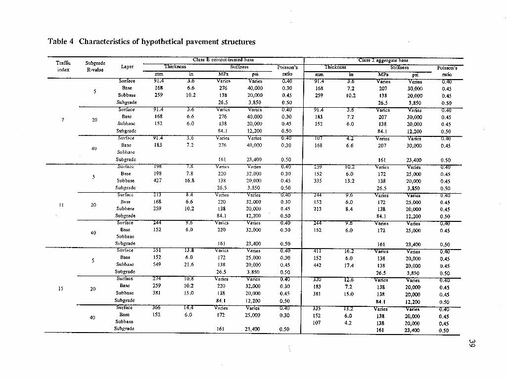
Table 4 Characteristics of hypothetical pavement structures .
Traffk Subgrade index R-value
Layer Class B cement-treated base
Thtckness Stiffness Poisson’s mm in MPa psi ratio
7
5
20
40
Surface
Base Subbase
Subgrade Surface
Base
Subbase
Subgrade Surface
Base Subbase
Subgrade Surface
91 4
16; 259
91 4 168 152
91 4
183
36
6:6 10.2
36
616 6.0
7.2
Vanes
276 138
26.5 Vanes
276 138
84.1 Vanes
276
Vanes 40,000 20,000
3,850 Vanes
40,000 20,000 12,200 Vanes
40~000
198 161 23,400
Vartzs Vartes
5 Base 198 7.8 220 32,000 0.30
Subbase 427 16.8 138 20,000 0.45
Subgrade Surface 213
26.5 3,850 Vanes Vanes
11 20 Base 168 4.6 220 32,000 0.30
Subbase 259 10.2 138 20,000 0.45
Subgrade Surface
Base Subbase
Subgrade Surface
Base
Subbase Subgrade Surface
Base
SlJhhJJ~il:
Subgrade Surface
Base Subbase
Subgrade
244 84.1
Vanes 12,200 Vanes
152 6.0 220 32,000 0.30
351
152 549
214
259
381
366
152
6.0
21.6
IO 8
10:2 15.0
14 4
6.;
161 Vanes
172 138
26.5 Vanes
220
138 84.1
Vanes
172
161
23,400 Vanes
25,000
20,000 3,850 Vanes
32,000 2Q,ow 12,200 Vanes
25,000
23,400
0.30
0.45 0.50 0 40 0:30 0.45
0.50 0 40
0:30
0.50
40
15
5
20
40
w
Class 2 aggregate base Thickness Stiffness Poisson’s r .
mm .
in MPa PS’ ratio 91 4
16;
36
7:2
Vanes Vanes 0 40
207 30,ooo 0:45
259 10.2 138 20,OuO 0.45
26.5 3,850 0.50 91 4
183
36
7:2
Vanes Vanes 0 40
207 30,000 0:45
152 6.0 138 20,OOu 0.45
84.1 12,200 0.50 42
6:6
Vanes Vanes 0 40
168 207 30,000 0:45
259
152 335
244 152 213
244
152
411
152 442
320
183 381
335
152 107
10 2
6.; 13.2
96 6:0 8.4
96
6:0
16 2
6.; 17.4
12 6
7.; 15.0
13 2
6.; 4.2
161 Vanes
172 138
26.5 Vanes
172 138
84.1 Vanes
172
161 Vanes
138 138
26.5 Vanes
138 138
84.1 Vanes
138 138 161
23,400 Vanes
25,000 20,000 3,850 Vanes 25,OCX.I 20,000 f 2,200 Vanes 25,000
23,400 Vanes
20,000 20,ooo 3,850 Vanes
20,000 20,m 12,200 Vanes
20,000 20,ooo 23,400
0.50 0 40 0:45 0.45 0.50
0.45 0.43 0.50 0 40 0:45
0.50 0 40
0145 0.45 0.50 0 40
0:45 0.45 0.50 0 40
0:45 0.45 0.50
t, w

40
Table 5 Location and climatic summary of California sites
Attribute Santa Barbara
Site
Daggett Blue Canyon
Latitude (“) 34.433 34.867
Elevation (feet) 3 586
Constant deep ground temperature (F)
Period
Average minimum daily air temperature (F)
Average maximum daily air temperature (F)
Average daily sunshine (%)
Average daily wind speed (mph)
62 70
1984-1993 1983, 19851993 1983-1988
48.8 53.2 43.9
70*7 81.5 58.8
67.9 81.3
60 . 11.2
--
39.283
1,609
57
65.3 1
43 .
Note: C = 5/9(F - 32); 1 mph = 1.61 km/h

41
Table 6 Selected temperature simulation parameters’
Layer Property Calibrated value
Thermal conductivity 0.8 BTU/hr-ft-F (unfrozen, frozen, freezing) I
Asphalt Heat capacity 0.22 BTU/lb-F (unfrozen and freezing)
concrete 1.2 BTU/lb-F (freezing)
Unit weight 145 pcf
Water con tent 27 0
Subgrade Dry density 120 pcf
Dry heat capacity 0.29 BTU/lb-F
Maximum allowable convection coefficient
3 BTU/hr ft2 F
Emissivity factor 0.85
Absorptivity factor 0.90
Other Geiger radiation factor A ( 0.77
Geiger radiation factor B 0.28
Vapor pressure 5 mm mercury
Cloud base factor for back radiation 0.85
aOnly English units are‘shown because the computer program and data files are expressed in English units.

42
Table 7 Temperature conversion factors and critical temperatures
Thickness of asphalt layer (in)
Parameter Santa Barbara
Site
Daggett Blue Canyon
TCF (to 19C) 1.176 0.989 0.883
Percent of damage in SC range about 19C 16.6 12.8 12.8
Critical temperature (C) 27 30 28 4
TCF (to critical temperature) 0.655 0.587 0.481
Percent of damage in 5C range about critical temperature
34.6 24.4 30.2
TCF (to 19C) 2.392 2.446 1.887
Percent of damage in 5C range hbout 19C 84 . 58 . 73 .
Critical temperature (C) 29 34 30 8
TCF (to critical temperature) 0.582 0.546 0.417
Percent of damage in 5C range about critical temperature
49.3 32.9 41.4

43
Table 8 Asphalt binder properties (after PAV) at 20c and 10 radkec
Asphalt suurce G* @Pa) G*sid &Pa) G*coslj @Pa) tans
AAA 3,347 2,542 2,177 1.168
AAB 6,677 4,444 4,983 0.892
AAC 7,809 5,200 5,825 0.893
AAD 4,292 3,144 2,923 1.076
AAF 20,902 12,114 17,035 0.711
AAG 22,165 16,336 14,984 1.090
AAK 7,558 5,306 5,382 0.986
AAM 7,757 4,614 6,235 0.740
Table 9 Adjusted R2 for the stiffness and fatigue-life regressions with binder loss modulus
Aggregate Void content (%)
Adjusted R2 for binder loss stiffness versus
Mix stiffness Mix fatigue life ’
RD 4 0.829 0.730
RD 7 0.897 0.864
RH 4 0.955 0.826
RH 7 0.927 0.885