FEDERAL RESERVE BANK OF DALLAS

INFLATION EXPECTATIONS, REAL INTEREST

RATE AND RISK PREMIUMS—EVIDENCE FROM BOND MARKET

AND CONSUMER SURVEY DATA

Dong Fu

Research DepartmentWorking Paper 0705

FEDERAL RESERVE BANK OF DALLAS

In�ation Expectations, Real Interest Rate and Risk

Premiums�Evidence from Bond Market and

Consumer Survey Data�

Dong Fuy

June 2007

Abstract

This paper extracts information on in�ation expectations, the real interest rate, and various

risk premiums by exploring the underlying common factors among the actual in�ation, Univer-

sity of Michigan consumer survey in�ation forecast, yields on U.S. nominal Treasury bonds, and

particularly, yields on Treasury In�ation Protected Securities (TIPS). Our �ndings suggest that

a signi�cant liquidity risk premium on TIPS exists, which leads to in�ation expectations that

are generally higher than the in�ation compensation measure at the 10-year horizon. On the

other hand, the estimated expected in�ation is mostly lower than the consumer survey in�ation

forecast at the 12-month horizon. Survey participants slowly adjust their in�ation forecasts

in response to in�ation changes. The nominal interest rate adjustment lags in�ation move-

ments too. Our model also edges out a parsimonious seasonal AR(2) time series model in the

one-step-ahead forecast of in�ation.

JEL classi�cation: E43, G12, C32

Key words: In�ation Expectations, Treasury In�ation Protected Securities (TIPS), Survey

In�ation Forecast, Kalman Filter

�I would like to thank Nathan Balke for continuous guidance and encouragement. I also gratefully acknowledge

comments and suggestions from Thomas Fomby, Esfandiar Maasoumi, Mark Wynne, Tao Wu, John Duca, Jahyeong

Koo, Jonathan Wright, seminar participants at the Federal Reserve Bank of Dallas, O¢ ce of the Comptroller of the

Currency and SERI, participants at the LAMES 2006 and the SEA 2006 annual meeting. The views expressed are

those of the author and should not be attributed to the Federal Reserve Bank of Dallas or the Federal Reserve System.yResearch Department, Federal Reserve Bank of Dallas and Southern Methodist University. Correspondence:

dong_fu@yahoo.com

1

1 Introduction

Timely and accurate estimates of in�ation expectations are gaining importance in monetary policy

as in�ation targeting, formal or informal, has become a widely adopted practice (Leiderman and

Svensson, 1995; Bernanke, Laubach, Mishkin and Posen, 1998). Speci�cally, they help monetary

authorities in setting the short term real interest rate at the appropriate level and provide observers

a tool to analyze whether a central bank�s in�ation targeting is credible or not.

Many economic indicators contain information on in�ation and expectations of future in�ation.

In macroeconomics, the Phillips curve has played a central role in relating future in�ation to current

real activities (Stock and Watson, 1999; Gali and Gertler, 1999). However, many of these real

macroeconomic variables are subject to routine revisions, sometimes rather signi�cant ones. These

revisions present serious problems for real time analysis and forecasting. Two other channels,

which are less subject to data revisions, have also been used to gauge in�ation expectations, namely,

survey in�ation forecasts and the term structure of interest rates. In the latter approach, in�ation

compensation, de�ned as the yield spread between nominal and indexed government bonds of the

same maturity, is often taken as a proxy for the expected future in�ation. However, surveys of

in�ation expectations tend to re�ect partial and incomplete updating in response to macroeconomic

news (Mankiw, Reis and Wolfers, 2003), while the simple in�ation compensation measure ignores

various risk premiums involved in bond pricing (Berger, Stortelder and Wurzburger, 2001). More

importantly, using these measures individually may not e¢ ciently capture the information on the

underlying in�ation process.

This paper seeks to use the information contained in di¤erent channels simultaneously in measur-

ing in�ation expectations. Ours is a dynamic factor model, which extracts information on in�ation

expectations, the real interest rate and risk premiums by exploring the underlying common fac-

tors among a group of observed variables, including the actual in�ation, University of Michigan

consumer survey in�ation forecast, yields on nominal Treasury bonds, and particularly, yields on

Treasury In�ation Protected Securities (TIPS). We use the Kalman �lter in maximum likelihood

estimation of the state variables that drive the in�ation and real interest rate processes. These state

variables include unobserved permanent and temporary components of the real interest rate; perma-

nent, temporary and seasonal components of the in�ation rate; idiosyncratic excess return factors

on T-bonds and TIPS, which represent risk premiums; and an idiosyncratic factor representing the

survey in�ation forecast error. Our sample spans from 1997, when TIPS were �rst issued, to 2003.

Our estimate of U.S. in�ation expectations, which incorporates information from both the survey

2

in�ation forecast and bond market, seems much more sensitive to negative shocks to the U.S. econ-

omy than both the survey in�ation forecast and the in�ation compensation suggest. At the 10-year

horizon, this estimate is generally higher than the in�ation compensation measure. On the other

hand, the estimated in�ation expectation is mostly lower than the University of Michigan consumer

survey in�ation forecast at the 12-month horizon. The �nding that 10-year in�ation expectations

are higher than the in�ation compensation suggests a signi�cant liquidity risk premium of TIPS over

nominal T-bonds. In our model, the di¤erence between the excess returns of 10-year T-bonds and

TIPS can be viewed as a proxy for the in�ation risk premium embodied in the 10-year T-bond yield.

We �nd the di¤erence to be negative in part of the sample period, pointing to a possible liquidity

risk premium of TIPS over T-bonds. Our �nding, thus, is consistent with Shen and Corning (2001),

Sack (2000, 2004), D�Amico, Kim and Wei (2007). Sack (2000, 2004) uses o¤-the-run T-bond yields

to better match up with the TIPS yields on a liquidity basis. However, using o¤-the-run T-bonds

in our model doesn�t eliminate the negative values. The implication is that there is a signi�cant

liquidity risk premium of TIPS over T-bonds, no matter whether the latter are on-the-run or o¤-

the-run. We also �nd that the expected real interest rate has trended downward since the end of

2000.

Innovations in the real interest rate and in�ation are found to be strongly negatively correlated,

implying that nominal interest rate adjustments lag the in�ation changes, which is consistent with

the �ndings of Barr and Campbell (1997), Pennacchi (1991) and Summers (1983). We also �nd

negative correlation between innovations in in�ation and the survey in�ation forecast error factor,

suggesting survey participants only partly adjust their forecasts in response to underlying in�ation

changes, in line with Keane and Runkle (1990), Mankiw, Reis and Wolfers (2003). In addition, we

�nd innovations in permanent and temporary real interest rates to be positively correlated, as are

innovations in permanent and temporary in�ation. Our estimated nominal term premium follows

the observed term spread closely.

The model o¤ers us the opportunity to combine the information from the bond market, survey

in�ation forecast and actual realized in�ation in conducting forecasts. First, the simple out-of-

sample forecast suggests that the real interest rate is likely to stay low as of yearend 2003, while

in�ation remains stable. Then we conduct one-step ahead out-of-sample forecasts of the in�ation

rate by incorporating new data observations at each step, but without re-estimating the model

parameters because of the considerable cost involved in such estimations. Our model seems to do a

little better than a parsimonious seasonal AR(2) time series model of in�ation, in terms of producing

a lower RMSE for the out-of-sample forecast period from January 2004 to December 2005.

3

Our modelling of T-bond and TIPS yields follows a rich literature, dating back to Fisher (1896),

of analyzing the relationship between in�ation and interest rate. However, here we draw a distinction

between our model and the popular A¢ ne Term Structure Model (ATSM) (Cox, Ingersoll and Ross,

1985; Dai and Singleton, 2000)1 . In ATSM, bond prices (yields) are linear functions of unobserved

state variables (or latent factors), which re�ect sources of uncertainty and are usually termed as

�level�, �slope� and �curvature� factors. D�Amico, Kim and Wei (2007) use such a three-factor

term structure model to study the informational content of TIPS. Meanwhile, it remains a di¢ cult

task to link these latent factors to macroeconomic dynamics, even with recent progress made by Wu

(2005), and Ang and Piazzesi (2003), among others. So instead of relying on ATSM, this paper

derives the bond price (yield) from the standard asset pricing equation (Cochrane, 2001; Balke and

Wohar, 2000 & 2002; Pennacchi 1991). Bond prices (yields) are functions of underlying factors with

explicit economic meanings� the real interest rate, in�ation, and idiosyncratic factors embodying

risk premiums. These factors follow mutually dependent processes and we assume conditional

homoskedasticity2 .

Methodology-wise, this paper is done in the same vein as Pennacchi (1991), which also expresses

bond prices and in�ation forecasts as linear functions of state variables such as the real interest

rate and in�ation, but includes only constants instead of time-varying idiosyncratic factors in the

equations. Our other novelty here is the use of TIPS to supplement traditional T-bonds, together

with the survey in�ation forecast, in estimating the underlying factors. TIPS and other forms

of in�ation indexed bonds provide additional information on the real interest rate and in�ation

compared with the traditional T-bonds (Deacon and Derry, 1994; Campbell and Shiller, 1996; Evans,

1998 and Emmons, 2000). Since U.S. TIPS�appearance, in�ation compensation has often been used

as a measure of expected in�ation (Kliensen and Schmid, 2004). This approach ignores various risk

premiums involved in bond pricing. Barr and Campbell (1997) estimate the expected future real

interest rate and in�ation rate from observed prices of U.K. nominal and indexed government bonds.

They too ignore both the real term premium and in�ation risk premium, while Brown and Schaefer

(1994) allow for the real term premium in estimating a real yield curve of the U.K. in�ation indexed

bond using ATSM. In this paper, we model the excess return on an n-period T-bond or TIPS as a

time-varying maturity-speci�c idiosyncratic factor, which incorporates both the real term premium

and the in�ation risk premium. In addition, we explicitly consider the seasonal factor contained

1Estimation is either based on GMM, as in Gibbons and Ramaswamy (1986) and Heston (1988); or maximum

likelihood, as in Pearson and Sun (1988), Gong and Remolona (1996).2Campbell and Viceira (2001) has a similar setting, although more akin to the ATSM.

4

in the non-seasonally adjusted Consumer Price Index used for the indexation of TIPS. We also

account for the TIPS indexation lag, as Barr and Campbell (1997) suggest, while early studies, such

as Brown and Schaefer (1994), assume perfect indexation.

The remainder of the paper is organized as follows. Section 2 explores bond price (yield)

equations for both indexed and nominal bonds from a standard asset pricing setting. Section 3

lays out the formula for the consumer survey in�ation forecast. Section 4 details the processes of

underlying dynamic factors that determine the behavior of observed variables. Section 5 describes

the state space model and the Kalman �lter technique used in estimation. Section 6 reports our

major �ndings. Section 7 forecasts the in�ation and real interest rate. Section 8 concludes.

2 Bond Price

2.1 General Bond Price

The standard asset pricing equation is

1 = Et[Mt+1Rt+1] (1)

where Mt+1 is the stochastic discount factor and Rt+1 is the real gross return from holding an asset

from time t to time t+ 1. When the asset is an n-period zero-coupon bond, (1) becomes

1 = Et

�Mt+1

�PtPt+1

��Qn�1;t+1Qn;t

��Qn;t is the nominal price at t of this bond, which matures at t+ n. Pt is the general price level at

t. So the bond price can be rewritten iteratively as

Qn;t = Et

" nYi=1

Mt+i

! nYi=1

Pt+i�1Pt+i

!Q0;t+n

#(2)

Q0;t+n is the nominal price of this bond at the maturity date t+n. For a nominal bond, we routinely

standardize Q0;t+n to 1. When Q0;t+n is indexed to re�ect general price level changes over time,

the bond becomes an in�ation indexed bond. In the following discussion, we assume all data are of

monthly frequency.

2.2 In�ation Indexed Bond Price

2.2.1 Fully Indexed Bond Price

For a fully indexed bond, we have

5

Q0;t+n = 1 �Pt+nPt

From (2), the price at time t of a n-period fully indexed zero-coupon bond, denoted by QRn;t, is

QRn;t = Et

" nYi=1

Mt+i

!#(3)

So this bond becomes a real bond. Under log normality, we have

logQRn;t = Et

"nXi=1

mt+i

#+1

2V art

"nXi=1

mt+i

#where mt = log (Mt). The yield to maturity of this real bond is the n-period real interest rate,

denoted by iRn;t.

iRn;t = ��1

n

�(Et

"nXi=1

mt+i

#+1

2V art

"nXi=1

mt+i

#)When n = 1, iR1;t is simply the expected one-period real interest rate

Et [rt+1] = iR1;t = �

�Et [mt+1] +

1

2V art [mt+1]

�When n > 1, iRn;t can be rewritten as

iRn;t =

�1

n

� nXi=1

Et [rt+i]��1

n

� nXi=j+1

nXj=1

Covt [mt+i;mt+j ] (4)

where�1n

�Pni=1Et [rt+i] is the average expected one-period real interest rate over the bond�s lifetime

and ��1n

�Pni=j+1

Pnj=1 Covt [mt+i;mt+j ] is the real term premium investors demand in order to

invest in the n-period real bond instead of the one-period real bond.

2.2.2 TIPS Price

Lately, in�ation indexed bonds have gained increasing popularity in a number of countries. In

reality, these bonds all deviate one way or another from the fully indexed bond. The U.S. TIPS

are a case in point. TIPS are coupon bonds, with both coupon payments within the term and

principal repayment at the maturity date indexed to re�ect the changes over time of the non-

seasonally adjusted Consumer Price Index (CPI). For convenience in analysis, we assume TIPS are

zero-coupon bonds. In fact, TIPS yields are routinely quoted on a zero-coupon basis in practice

(for example, in McCulloch and Kochin, 2000; see data appendix A.2).

6

Assume an n-period zero-coupon TIPS is issued at t. Ideally, at its maturity date t+ n, TIPS�

nominal price should re�ect the CPI level change between the issuing date t and the maturity date

t+n. In reality, TIPS are indexed to the CPI with a short indexation lag of 3 months3 (We assume

n > 3 holds for TIPS in all following discussions). So,

Q0;t+n = 1 �Pt+n�3Pt�3

From (2), the price at t of a n-period TIPS, denoted by QLn;t, is

QLn;t = Et

" nYi=1

Mt+i

!�Pt+n�3Pt+n

��PtPt�3

�#(5)

Similar to Barr and Campbell (1997), we assume Et(Pt) = Pt4 . Thus (5) becomes

QLn;t =

�PtPt�3

�Et

" nYi=1

Mt+i

!=

3Yi=1

Pt+n+1�iPt+n�i

!#Under log normality, with mt = log (Mt) and �t = log (Pt=Pt�1), the yield to maturity of TIPS is

iLn;t =

�1

n

� nXi=1

Et [rt+i]��1

n

� nXi=j+1

nXj=1

Covt [mt+i;mt+j ]�

�1

n

�log

�PtPt�3

�+

�1

n

� 3Xi=1

Et [�t+n+1�i]�

�1

n

�(1

2V art

"3Xi=1

�t+n+1�i

#� Covt

"nXi=1

mt+i;3Xi=1

�t+n+1�i

#)(6)

Unlike the fully indexed bond, TIPS is exposed to a small amount of in�ation risk due the

indexation lag. Appendix B compares TIPS with the fully indexed bond in more details. Next, we

de�ne an idiosyncratic excess return factor �n;t on TIPS, which contains all the variance-covariance

terms in (6). We assume it is dependent on maturity n and time varying, similar to Balke and

Wohar (2000, 2002). So the TIPS yield can be rewritten as

iLn;t = ��1

n

�log

�PtPt�3

�+

�1

n

� nXi=1

Et [rt+i] +

�1

n

� 3Xi=1

Et [�t+n+1�i] + �n;t (6�)

3Strictly speaking, the TIPS indexation lag is 2.5 months. The indexation lag for the U.K. in�ation indexed bond

is 8 months. See Barr and Campbell (1997), Deacon and Derry (1994), McCulloch and Kochin (2000) for details.4 In expectation models, it is customary to assume a random variable Xt�s conditional expectation Et (Xt) = Xt.

In other words, Xt is observed at t. However, in reality, Xt is usually not observed until some time after t. For

example, CPI is normally observed with a lag. In fact, it is precisely because of this lag that TIPS is indexed to CPI

with a lag of 3 months in practice.

7

2.3 Nominal Treasury Bond Price

Because Q0;t+n = 1 for a nominal bond, from (2), the price of an n-period nominal T-bond at t,

still denoted by Qn;t, is

Qn;t = Et

" nYi=1

Mt+i

!=

nYi=1

Pt+iPt+i�1

!#(7)

Under log normality, the yield to maturity of this n-period nominal t-bond is

in;t =

�1

n

� nXi=1

Et [rt+i]��1

n

� nXi=j+1

nXj=1

Covt [mt+i;mt+j ] +

�1

n

� nXi=1

Et [�t+i]�

�1

n

�(1

2V art

"nXi=1

�t+i

#� Covt

"nXi=1

mt+i;nXi=1

�t+i

#)(8)

Compared with TIPS yield, nominal T-bond yield covers more completely the expected in�ation

and in�ation risk premium during the entire lifetime of n periods. Appendix B provides more

details. We de�ne a time-varying and maturity-speci�c idiosyncratic excess return factor �n;t on a

nominal T-bond as containing all the variance-covariance terms in (8), similar to the case of TIPS.

So a nominal T-bond yield can be rewritten as

in;t =

�1

n

� nXi=1

Et [rt+i] +

�1

n

� nXi=1

Et [�t+i] + �n;t (8�)

2.4 In�ation Compensation

From (6�) and (8�), in�ation compensation, de�ned as the di¤erence between the yield of a nominal

T-bond and the yield of a TIPS of the same maturity (Sack, 2000; Kliensen and Schmid, 2004), is

in;t � iLn;t =�1

n

�log

�PtPt�3

�+

�1

n

� n�3Xi=1

Et [�t+i] +��n;t � �n;t

�(9)

We can see it contains three parts. First, existing price change between t � 3 and t. Second,

the expected in�ation between t and t + n � 3. The sum of the two is a proxy for the expected

in�ation during the bonds�entire lifetime from t to t + n. The third part��n;t � �n;t

�stands for

the di¤erence between the excess return on the nominal T-bond and the excess return on the TIPS.

8

�n;t � �n;t

= ��1

n

�(1

2V art

"nXi=1

�t+i

#� Covt

"nXi=1

mt+i;nXi=1

�t+i

#)�(

��1

n

�(1

2V art

"3Xi=1

�t+n+1�i

#� Covt

"nXi=1

mt+i;3Xi=1

�t+n+1�i

#))(10)

Here, ��1n

� �12V art [

Pni=1 �t+i]� Covt [

Pni=1mt+i;

Pni=1 �t+i]

is the risk premium due to in�ation

uncertainty in n periods. ��1n

�n12V art

hP3i=1 �t+n+1�i

i� Covt

hPni=1mt+i;

P3i=1 �t+n+1�i

iois

the risk premium due to in�ation uncertainty during the indexation lag period. As long as n is

much larger than 3, the �rst term dominates the second term.

2.5 Summary

According to (6�), the TIPS yield is a function of the expected real short interest rate Et [rt+i],

expected in�ation Et [�t+i] and the excess return �n;t. And according to (8�), the nominal T-bond

yield is a function of Et [rt+i], Et [�t+i] and the excess return �n;t. The time varying excess returns

�n;t and �n;t incorporate both real term premium and in�ation risk premium (see appendix B for

details). The measure of in�ation risk premium is particularly important. One of the major

reasons for issuing the indexed bond is that it is supposedly shielded from the in�ation risk. So

the Treasury department doesn�t have to pay an in�ation risk premium, resulting in a lower cost

of �nancing government debts. Equally important, once we have an estimate of the in�ation risk

premium, we can screen it out from the in�ation compensation measure to obtain a more precise

estimate of underlying expected in�ation.

Barr and Campbell (1997) directly model the prices, instead of the yields, of U.K. nominal

and indexed bonds as functions of the expected real interest rate and the expected in�ation rate.

However, they assume the expected real holding period returns on both nominal and indexed bonds

at any point in time are the same as the short term real interest rate. This actually contains two

assumptions. First, the real holding period return equals the short term real interest rate� the log

pure expectation hypothesis of the real interest rate, so there is no real term premium. Second,

expected real holding period returns on nominal bonds equal returns on indexed bonds, implying

zero in�ation risk premium. As no risk premium is considered, their model equates to assuming

the variance and covariance terms in our bond price equations are all zeros.

In reality, taxation a¤ects the perception of returns and risks involved in pricing TIPS and

nominal T-bonds. However, we choose not to model the tax e¤ects explicitly in this paper, because

9

our focus is on the common factors behind in�ation and the real interest rate, based on both TIPS

and nominal T-bonds yields. Fitting of either type of bond yields is of secondary importance. In

any event, tax e¤ects will only show up in the discount factor (real interest rate), but will not a¤ect

the in�ation process. If the tax treatment of investing in TIPS is the same as that of investing

in nominal T-bonds, we can simply regard the discount factor mt as the after-tax discount factor,

taking into account that the tax rate is also time varying. Similarly, the real interest rate rt can

be simply viewed as the after-tax real interest rate. If tax treatments di¤er, we argue that the

common underlying discount factor (real interest rate) movement should still be picked up by mt

(rt) in our setup while the di¤erential taxation e¤ect is pushed into the idiosyncratic excess return

factor of either TIPS or nominal T-bonds. Another practical di¢ culty in modeling the tax e¤ect is

that di¤erent investors face di¤erent marginal tax rates on investing in the bond market. Anyway,

considering that TIPS only make up a small portion of the U.S. government bond market at the

moment, di¤erential taxation e¤ects overall should be small.

3 Survey In�ation Forecast

Survey in�ation forecasts have been frequently used as benchmarks for measuring in�ation expec-

tations. Examples include the in�ation forecast from the Federal Reserve Bank of Philadelphia�s

survey of professional forecasters (Croushore, 1993; Zarnowitz and Braun, 1992; Giordani and Soder-

lind, 2002), the University of Michigan consumer survey in�ation forecast (Curtin, 1996), and the

Blue Chip forecast of in�ation. Thomas (1999) and Mehra (2002) summarize recent developments

in these survey in�ation forecasts.

In this paper, we use the University of Michigan consumer survey in�ation forecast, which is

available monthly and has seen wide usage in practice (see data appendix A.3). Keane and Runkle

(1990) suggest surveys based on polling non-professional forecasters, who lack the incentive to com-

pile accurate forecasts compared with professional forecasters, may not rationally utilize all available

information. As non-professional survey participants are usually not as �nancially liable as profes-

sionals, they can be tardy in updating their forecasts, thus leading to potentially persistent forecast

errors. Mankiw, Reis and Wolfers (2003) also �nd surveys of in�ation expectations tend to re�ect

partial and incomplete updating in response to macroeconomic news. Accordingly, we model the

consumer survey in�ation forecast at t for future n periods, denoted by �surveyn;t , as

�surveyn;t =1

nEt

"nXi=1

�t+i

#+ en;t (11)

10

We assume the persistent forecast error is re�ected in an idiosyncratic factor en;t, which is dependent

on the forecasting horizon n and is time varying. Thus, the consumer survey in�ation forecast is a

function of expected in�ation Et [�t+i] and the forecast error factor en;t.

4 Underlying Factor Processes

So far, we have shown that the observed TIPS yield, T-bond yield and survey in�ation forecast are

all determined by unobserved factors. Among them, common factors Et [�t+i] and Et [rt+i] are

shared by multiple observed variables. By exploring the cross-equation restriction imposed by these

common factors on the observed variables, we can extract information on the underlying factors.

To do so, we need to put more structure on the factors�generating processes.

We assume the short term (one-month) real interest rate consists of a permanent (trend) com-

ponent rpt and a temporary (cyclical) component rat

rt = rpt + r

at (12)

rpt follows a random walk and rat follows AR(2)

rpt = rpt�1 + vrpt (13)

rat = �ra1 � rat�1 + �ra2 � rat�2 + vrat (14)

Because TIPS indexation is based on the nonseasonally-adjusted CPI5 , we use the nonseasonally-

adjusted CPI month-over-month in�ation in the model. Following Harvey (1989, 1990, 1993),

Koopman, Harvey, Doornik and Shephard (2000), the CPI in�ation consists of a permanent (trend)

component �pt , a temporary (cyclical) component �at and a seasonal component �

st

�t = �pt + �

at + �

st (15)

�pt follows a random walk and �at follows AR(2)

�pt = �pt�1 + v�pt (16)

�at = ��a1 � �at�1 + ��a2 � �at�2 + v�at (17)

The seasonal component �st can be represented by t, which evolves according to

5�Summary of Marketable Treasury In�ation-Indexed Securities�(http://www.publicdebt.treas.gov/gsr/gsrlist.html)

11

0BBBBBBBBBBBBBBBBB@

t

t�1

:

:

:

t�9

t�10

1CCCCCCCCCCCCCCCCCA

=

0BBBBBBBBBBBBBBBBB@

�1 �1 : : : �1 �1

1

:

:

:

1

1 0

1CCCCCCCCCCCCCCCCCA

0BBBBBBBBBBBBBBBBB@

t�1

t�2

:

:

:

t�10

t�11

1CCCCCCCCCCCCCCCCCA

+

0BBBBBBBBBBBBBBBBB@

v t

0

:

:

:

0

0

1CCCCCCCCCCCCCCCCCA

(18)

So the process for in�ation can be rewritten as

�t = �pt + �

at + t (15�)

We assume the excess return factors in the nominal T-bond and TIPS yields follow AR(2).

�n;t = ��n;1 � �n;t�1 + �

�n;2 � �n;t�2 + v

�n;t (19)

�n;t = ��n;1 � �n;t�1 + ��n;2 � �n;t�2 + v�n;t (20)

So does the survey in�ation forecast error factor.

en;t = �en;1 � en;t�1 + �en;2 � en;t�2 + ven;t (21)

5 State Space Model

Now we build a state space model following Harvey (1993), Hamilton (1994) and Harvey, Koopman

and Shephard (2004). Appendix C.1 provides an overview of the state space model. In our case, the

observed variables Yt include the 3-month T-bill yield, 10-year T-bond yield, 10-year TIPS yield, 12-

month in�ation forecast from the University of Michigan consumer survey, as well as actual monthly

in�ation (see data appendix A for more detailed descriptions). All data are monthly and quoted in

annual rates. The sample period is from January 1997, when TIPS were �rst issued, to December

2003. We choose to work with demeaned data Yt, di¤erent from Pennacchi (1991) and Barr and

Campbell (1997)6 . The resulting state space model is more parsimonious as it contains no intercept

in either the observation equation or the state equation.6Pennacchi (1991) models bond prices and survey in�ation forecasts as functions of expected real interest rate and

in�ation in a similar state space setting. He also de�nes state variables in terms of deviations from their unconditional

means, but retains observed variables without demeaning. In comparison, Barr and Campbell (1997) impose trend-

12

5.1 State Equation

Under the assumption of rational expectations, and using equations (12) through (21), we transform

the initial unobserved underlying factors Et [rt+i] contained in (6�) and (8�), Et [�t+i] in (6�), (8�)

and (11), �n;t in (6�), �n;t in (8�) and en;t in (11) into an expanded state vector, which evolves

according to the following state equation:

0BBBBBBBBBBBBBBBBBBBBBBBBBBBBBBBBBBBBBBBBBBBBBBBBBBBBB@

rpt

�pt

t

t�1

:::

t�10

rat

�at

�a3m;t

�a10yr;t

�a10yr;t

ea12m;t

rat�1

�at�1

�a3m;t�1

�a10yr;t�1

�a10yr;t�1

ea12m;t�1

1CCCCCCCCCCCCCCCCCCCCCCCCCCCCCCCCCCCCCCCCCCCCCCCCCCCCCA

=

0BBBBBBBBBBBBBBBBBBBBBBBBBBBBBBBBBBBBBBBBBBBBBBBBBBBBB@

1

1

�1 ::: �1 �1

1

:::

1 0

�ra1 �ra2

: :

: :

: :

: :

�ea12m;1 �ea12m;2

1

:

:

:

:

1

1CCCCCCCCCCCCCCCCCCCCCCCCCCCCCCCCCCCCCCCCCCCCCCCCCCCCCA

�

0BBBBBBBBBBBBBBBBBBBBBBBBBBBBBBBBBBBBBBBBBBBBBBBBBBBBB@

rpt�1

�pt�1

t�1

t�2

:::

t�11

rat�1

�at�1

�a3m;t�1

�a10yr;t�1

�a10yr;t�1

ea12m;t�1

rat�2

�at�2

�a3m;t�2

�a10yr;t�2

�a10yr;t�2

ea12m;t�2

1CCCCCCCCCCCCCCCCCCCCCCCCCCCCCCCCCCCCCCCCCCCCCCCCCCCCCA

+

0BBBBBBBBBBBBBBBBBBBBBBBBBBBBBBBBBBBBBBBBBBBBBBBBBBBBB@

vrpt

v�pt

v t

0

0

0

vrat

v�at

v�a3m;t

v�a10yr;t

v�a10yr;t

vea12m;t

0

0

0

0

0

0

1CCCCCCCCCCCCCCCCCCCCCCCCCCCCCCCCCCCCCCCCCCCCCCCCCCCCCA

St = F � St�1 + Vt (22)

with Vt s N(0; Q). As we are particularly interested in the relationship among various factors, we

want to impose a minimum number of restrictions on Q. The only restriction on Q is that there

stationary AR(1) processes directly on the log expected in�ation and expected real interest rate, which are then

estimated from cross section data of observed bond prices at a particular time t. Their data are not demeaned

either. The intercepts of the asset pricing equations based on the underlying in�ation and real short interest rate are

identi�ed as part of the AR(1) processes.

13

is no correlation between the innovation in in�ation�s seasonal factor v t and innovations in other

factors.

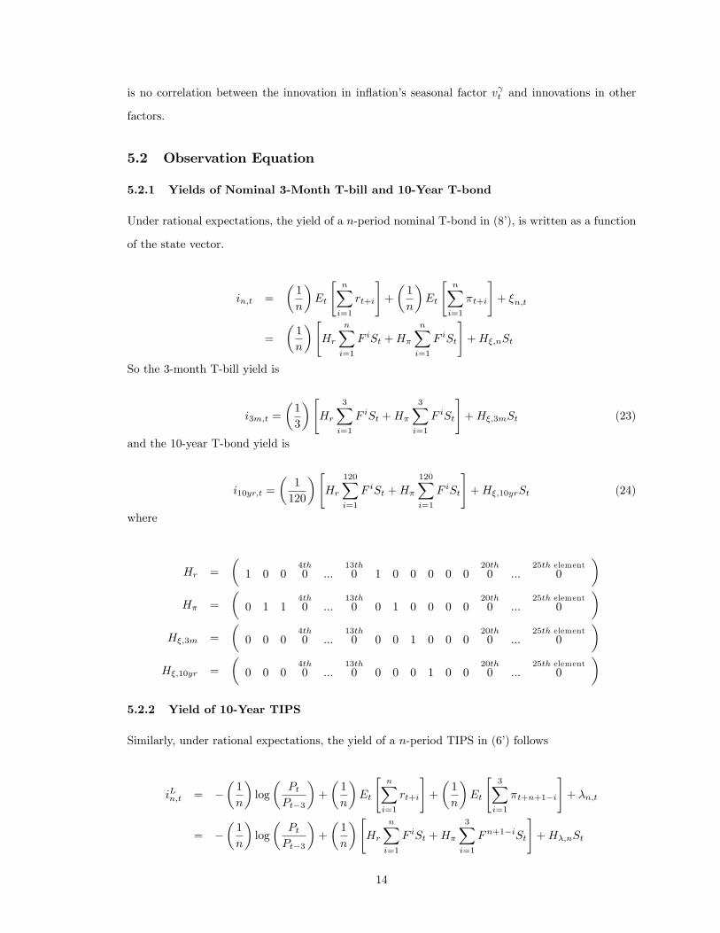
5.2 Observation Equation

5.2.1 Yields of Nominal 3-Month T-bill and 10-Year T-bond

Under rational expectations, the yield of a n-period nominal T-bond in (8�), is written as a function

of the state vector.

in;t =

�1

n

�Et

"nXi=1

rt+i

#+

�1

n

�Et

"nXi=1

�t+i

#+ �n;t

=

�1

n

�"Hr

nXi=1

F iSt +H�

nXi=1

F iSt

#+H�;nSt

So the 3-month T-bill yield is

i3m;t =

�1

3

�"Hr

3Xi=1

F iSt +H�

3Xi=1

F iSt

#+H�;3mSt (23)

and the 10-year T-bond yield is

i10yr;t =

�1

120

�"Hr

120Xi=1

F iSt +H�

120Xi=1

F iSt

#+H�;10yrSt (24)

where

Hr =

�1 0 0

4th0 :::

13th0 1 0 0 0 0 0

20th0 :::

25th element0

�H� =

�0 1 1

4th0 :::

13th0 0 1 0 0 0 0

20th0 :::

25th element0

�H�;3m =

�0 0 0

4th0 :::

13th0 0 0 1 0 0 0

20th0 :::

25th element0

�H�;10yr =

�0 0 0

4th0 :::

13th0 0 0 0 1 0 0

20th0 :::

25th element0

�

5.2.2 Yield of 10-Year TIPS

Similarly, under rational expectations, the yield of a n-period TIPS in (6�) follows

iLn;t = ��1

n

�log

�PtPt�3

�+

�1

n

�Et

"nXi=1

rt+i

#+

�1

n

�Et

"3Xi=1

�t+n+1�i

#+ �n;t

= ��1

n

�log

�PtPt�3

�+

�1

n

�"Hr

nXi=1

F iSt +H�

3Xi=1

Fn+1�iSt

#+H�;nSt

14

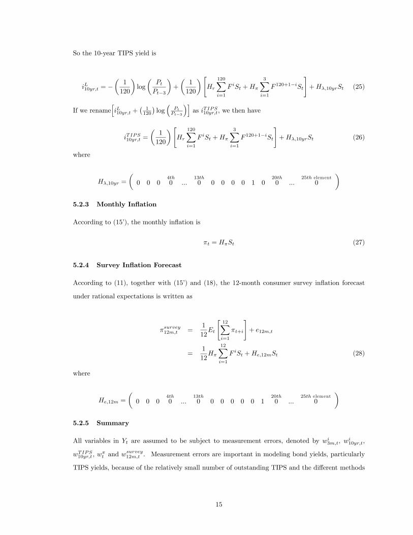
So the 10-year TIPS yield is

iL10yr;t = ��1

120

�log

�PtPt�3

�+

�1

120

�"Hr

120Xi=1

F iSt +H�

3Xi=1

F 120+1�iSt

#+H�;10yrSt (25)

If we renamehiL10yr;t +

�1120

�log�

PtPt�3

�ias iTIPS10yr;t, we then have

iTIPS10yr;t =

�1

120

�"Hr

120Xi=1

F iSt +H�

3Xi=1

F 120+1�iSt

#+H�;10yrSt (26)

where

H�;10yr =

�0 0 0

4th0 :::

13th0 0 0 0 0 1 0

20th0 :::

25th element0

�

5.2.3 Monthly In�ation

According to (15�), the monthly in�ation is

�t = H�St (27)

5.2.4 Survey In�ation Forecast

According to (11), together with (15�) and (18), the 12-month consumer survey in�ation forecast

under rational expectations is written as

�survey12m;t =1

12Et

"12Xi=1

�t+i

#+ e12m;t

=1

12H�

12Xi=1

F iSt +He;12mSt (28)

where

He;12m =

�0 0 0

4th0 :::

13th0 0 0 0 0 0 1

20th0 :::

25th element0

�

5.2.5 Summary

All variables in Yt are assumed to be subject to measurement errors, denoted by wi3m;t, wi10yr;t,

wTIPS10yr;t , w�t and w

survey12m;t . Measurement errors are important in modeling bond yields, particularly

TIPS yields, because of the relatively small number of outstanding TIPS and the di¤erent methods

15

used in estimating the yield curve in practice7 . However, the measurement error in bond yields

may be eclipsed by idiosyncratic excess return factors. Similarly, measurement errors�e¤ect on the

survey in�ation forecast may be small as the idiosyncratic factor is likely to pick up most of the

variation. On the other hand, measurement errors may a¤ect observed in�ation to a larger extent

as no idiosyncratic factor is there to pick up the residual variation in data. Now the combined

observation equation in the state space model is0BBBBBBBBBB@

i3m;t

i10yr;t

iTIPS10yr;t

�t

�survey12m;t

1CCCCCCCCCCA=

0BBBBBBBBBB@

�13

�(Hr +H�)

P3i=1 F

i +H�;3m�1120

�(Hr +H�)

P120i=1 F

i +H�;10yr�1120

� �HrP120

i=1 Fi +H�

P3i=1 F

120+1�i�+H�;10yr

H��112

�H�P12

i=1 Fi +He;12m

1CCCCCCCCCCA� St +

0BBBBBBBBBB@

wi3m;t

wi10yr;t

wTIPS10yr;t

w�t

wsurvey12m;t

1CCCCCCCCCCA

Yt = H � St +Wt (29)

withWt s N(0; R). R is assumed to be diagonal, indicating no cross correlation among observation

errors.

5.3 Estimation

The state space model usually has a large number of unknown parameters. However, in this model,

the H matrix in the observation equation (29) involves only constant vectors such as Hr and H�,

except the unknown F matrix, which also belongs to the state equation (22). This H matrix in fact

puts strong cross-equation restrictions on parameters in both the state and observation equations.

These restrictions go a long way in helping to achieve identi�cation. We estimate the state space

model using a combination of the EM algorithm (Watson and Engle, 1983) and the traditional

Maximum Likelihood estimation method (Hamilton, 1994). Appendix C.2 covers the estimation

technique in detail. We are able to achieve convergence in the maximization process. Appendix C.3

provides goodness of �t statistics. In general, the model performs reasonably well. Appendix C.4

details the estimated AR(2) coe¢ cients. The excess return factors of the 10-year T-bond yield and

TIPS yield are highly persistent, more than the excess return factor in the 3-month T-bill yield. The

forecast error factor in the survey in�ation forecast is also fairly persistent. We �nd low persistence

in the temporary real interest rate and temporary in�ation.

7Our dynamic factor model in the state space form o¤ers the �exibility to model measurement errors in bond

yields, similar to Pennacchi (1991). In comparison, A¢ ne Term Structure Model (ATSM) is more restrictive in that

the number of bonds subject to measurement errors is assumed to be the same as the number of underlying factors.

16

6 Major Findings

6.1 Correlations of Innovations in the State Factors

By examining the variance-covariance/correlation matrix Q of the state equation in table 1, we can

establish the relationship among in�ation, the real interest rate and survey in�ation forecast. The

variance-covariance terms are on and below the diagonal, while the correlation coe¢ cients are above

the diagonal.

Table 1

Variance-covariance/Correlation Matrix Q of the State Equation

vrpt v�pt v t vrat v�at v�a3m;t v�a10yr;t v�a10yr;t vea12m;t

vrpt 0.4602 -0.85 0 0.71 -0.58 -0.49 -0.49 -0.98 0.87

v�pt -0.3403 0.3514 0 -0.72 0.69 -0.04 0.06 0.81 -0.98

v t 0 0 0.0000 0 0 0 0 0 0

vrat 0.7299 -0.6491 0 2.3229 -0.98 0.01 -0.09 -0.65 0.83

v�at -0.6235 0.6509 0 -2.3643 2.5124 -0.21 -0.07 0.52 -0.79

v�a3m;t -0.0843 -0.0056 0 0.0042 -0.0862 0.0656 0.83 0.51 0.01

v�a10yr;t -0.1170 0.0121 0 -0.0479 -0.0380 0.0758 0.1256 0.60 -0.05

v�a10yr;t -0.4536 0.3288 0 -0.6713 0.5629 0.0897 0.1441 0.4647 -0.82

vea12m;t 0.1891 -0.1865 0 0.4035 -0.4030 0.0004 -0.0057 -0.1790 0.1029

An innovation in the permanent real interest rate is highly negatively correlated with innovations

in both permanent in�ation (-0.85) and temporary in�ation (-0.58). In addition, an innovation in

the temporary real interest rate is highly negatively correlated with innovations in both permanent

in�ation (-0.72) and temporary in�ation (-0.98). These suggest that the real interest rate and

in�ation tend to move in opposite directions. An increase in the real interest rate typically coincides

with a decrease in in�ation. Or alternatively, an increase in in�ation coincides with a decrease in

the real interest rate, re�ected by the nominal interest rate not increasing as much as in�ation. So

in general, the nominal interest rate doesn�t adjust one for one in response to, but lags behind, the

in�ation movement. This is consistent with the �ndings of Barr and Campbell (1997) based on

U.K. bond data, Pennacchi (1991) based on U.S. data, and other earlier studies such as Summers

(1983).

17

Of particular interest is that an innovation in either permanent in�ation or temporary in�ation

is highly negatively correlated (-0.98 and -0.79 respectively) with an innovation in the survey in-

�ation forecast error factor. So a shock that increases in�ation is cancelled out by a shock to the

survey in�ation forecast error factor in the opposite direction. This suggests that in�ation survey

participants are slow to adjust to changes in underlying actual in�ation, which is consistent with

our initial assumption that persistent forecast errors exist among survey participants. As pointed

out earlier, the real interest rate and in�ation tend to move in opposite directions. So it is not

surprising that an innovation in either the permanent or the temporary real interest rate is highly

positively correlated (0.87 and 0.83 respectively) with an innovation in the survey in�ation forecast

error factor.

Innovations in excess returns in the 3-month T-bill and 10-year T-bond are highly positively

correlated (0.83). They are also positively correlated (0.51 and 0.60 respectively) with an innovation

in the excess return in 10-year TIPS, although to a lesser extent than the correlation between

themselves. This is consistent with the fact that short and long nominal bonds are subject to the

same set of real interest risk and in�ation risk, while TIPS are largely shielded from in�ation risk.

Innovations in the permanent and temporary real interest rate are highly positively correlated

(0.71). So a shock that increases the permanent real interest rate coincides with an increase in the

temporary real interest rate. The real interest rate is likely to show high volatility. The correlation

between innovations in permanent in�ation and temporary in�ation is also highly positive (0.69).

So a shock that increases permanent in�ation coincides with an increase in temporary in�ation.

In�ation, as a sum of the permanent, temporary and seasonal components, is likely to show high

volatility too. Considering the data are of monthly frequency, it is not surprising that the real

interest rate and in�ation tend to show high volatility.

Even though we have imposed only the minimum restriction on matrix Q of no correlation

between innovations in the seasonal factor of in�ation and other factors, our model establishes

reasonable relationships among major factors. Appendix C.5 performs a robustness check on these

relationships, with additional restrictions that an innovation in the survey in�ation forecast error

factor is uncorrelated with innovations in other factors. Our �ndings on the relationships among

major factors, particularly between in�ation and the real interest rate, are untouched. However,

with the additional restrictions, we lose the interesting �nding that survey participants adjust to

in�ation changes with considerable inertia. So we prefer the current model in general.

18

6.2 Contributions of Factors to Observed Variables

Equation 30 estimates Y t, given the �ltered state vector Stjt, which is based on the information up

to time t.

Y t = H � Stjt (30)0BBBBBBBBBB@

i3m;t

i10yr;t

iTIPS10yr;t

�t

�survey12m;t

1CCCCCCCCCCA=

0BBBBBBBBBB@

H1

H2

H3

H4

H5

1CCCCCCCCCCA� Stjt

Now we can analyze the contributions of the state vector to each observed variable. Because our

model uses demeaned data, all contributions discussed here need to be interpreted as made toward

the observed variables relative to their means.

First, we look at contributions of the state vector to observed in�ation. From (30), we have

�t = H4 �Stjt = H� �Stjt, which can be decomposed into contributions of permanent, temporary and

seasonal in�ation to observed in�ation �t. Figure 1 indicates that the seasonal component explains

only a minor part of �t, when compared with permanent and temporary in�ation combined. Figure 2

suggests that permanent in�ation and temporary in�ation tend to move together, which is consistent

with the positive correlation between innovations in permanent and temporary in�ation. This leads

to high volatility of in�ation, particularly in the post-1999 period in our sample. Temporary in�ation

explains more of this volatility than permanent in�ation.

Then, we analyze the contributions of the state vector to interest rates. From (30), we have

i3m;t = H1 � Stjt, which can be decomposed into contributions of the real interest rate, in�ation and

excess return to the observed i3m;t. From �gure 3, we can see the 3-month T-bill yield�s movement

is largely due to the real interest rate, consistent with the �nding by Mishkin (1990a) that, at the

shorter end, the term structure of nominal interest rates contains a great deal of information about

the real term structure. Meanwhile, contributions of the real interest rate and in�ation tend to move

in opposite directions. For example, immediately after the 9/11 terrorist attack, the real interest

rate shot up while in�ation dropped sharply, keenly re�ecting the market sentiment then. This is

consistent with our earlier �nding of negative correlation between innovations in the real interest rate

and in�ation. Furthermore, the permanent real interest rate explains more of the 3-month T-bill

yield�s movement than the temporary real interest rate (Figure 4), while neither the permanent nor

the temporary in�ation seems to explain much of the variation in the 3-month T-bill yield (Figure

19

5). The latter is again consistent with Mishkin (1990a)�s �nding that the term structure of nominal

interest rates for maturities of six months or less provides little information about the future path

of in�ation.

From (30), we have i10yr;t = H2 � Stjt, which can be decomposed into contributions of the real

interest rate, in�ation and excess return to the observed i10yr;t. Figure 6 shows contributions of

the real interest rate and in�ation still tend to move in opposite directions. However, in�ation�s

contribution to the 10-year T-bond yield is more pronounced than its contribution to the 3-month

T-bill yield. This is consistent with Mishkin (1990a, 1990b) and Fama (1990)�s �ndings that there

is substantial information in the longer maturity term structure about future in�ation. The short

term nominal interest rate mostly re�ects the real interest rate �uctuation, while the long term

nominal interest rate contains more information on underlying in�ation. In�ation�s contribution to

the 10-year T-bond yield is mostly due to permanent in�ation (Figure 7) and the real interest rate�s

contribution is largely due to the permanent real interest rate (Figure 8). In addition, a signi�cant

portion of the movement in the 10-year T-bond yield is explained by the idiosyncratic excess return

factor. Notably, since 2001, the idiosyncratic factor has trended up (Figure 6).

Similarly, iTIPS10yr;t = H3�Stjt can be decomposed into contributions of the real interest rate, in�ation

and excess return to the observed iTIPS10yr;t. As Figure 9 shows, in�ation�s contribution is negligible.

This is only natural, considering that the TIPS is shielded for the most part from price changes.

The TIPS yield�s movement is accounted for by the real interest rate (almost entirely due to the

permanent real interest rate in turn) and the idiosyncratic excess return factor. This idiosyncratic

factor has trended up since 2001, just as the case with the idiosyncratic factor in the 10-year T-bond

yield.

Finally, we look at contributions of the state vector to the survey in�ation forecast. From

(30), we have �survey12m;t = H5 � Stjt, which can be decomposed into contributions of in�ation and the

idiosyncratic forecast error factor to the observed �survey12m;t . Figure 10 indicates there is a signi�cant

forecast error. It tends to move in the opposite direction of in�ation, which is consistent with the

negative correlation found between innovations to in�ation and the forecast error factor. Figure 11

further suggests that permanent in�ation carries more weight than temporary in�ation in the survey

in�ation forecast.

6.3 Expected In�ation Based on Filtering

From (22) and (29), we derive the expected future in�ation at t+k based on the information available

at t as

20

Et [�t+k] = Et�H�St+k + w

�t+k

�= H� � F kStjt

So the average expected in�ation for future n months8 is de�ned as

�en =

�1

n

�H�

nXk=1

F kStjt

Figure 12 shows that over our sample there is little di¤erence between the expected future

in�ation at the 12-month horizon and that at the 10-year horizon. Figure 13 compares our measure

of expected 12-month in�ation with the 12-month in�ation forecast from the University of Michigan

consumer survey. Our estimated series follows the survey in�ation forecast�s general trend, but

remains lower than the survey in�ation forecast most of the time. Particularly, when there is a sharp

downturn in the consumer survey forecast of 12-month in�ation, our measure, which incorporates

additional bond market information, tends to predict an even steeper decline in future in�ation. For

example, it showed a greater drop in the aftermath of 9/11, and again in mid 2002, than the survey

in�ation forecast. These suggest survey participants may be slow to adjust their forecast, consistent

with our �nding of negative correlation between innovations to in�ation and the survey forecast error.

Figure 14 compares our measure of 10-year expected in�ation based on the information at time t

with the in�ation compensation measure, i.e., the yield spread between 10-year nominal T-bond and

10-year TIPS. Contrary to the case at the 12-month horizon, our measure of 10-year expected

in�ation has been generally higher than in�ation compensation since 1998. Again, it picked up a

much sharper downturn than the in�ation compensation measure did after 9/11 and in mid 2002.

In general, our estimated expected in�ation seems to be more sensitive to negative shocks to the

economy than both the in�ation survey forecast and in�ation compensation suggest.

6.4 In�ation Risk Premium vs. Liquidity Risk Premium

From (9), in�ation compensation at the 10-year horizon is

i10yr;t � iL10yr;t =�1

120

�log

�PtPt�3

�+

�1

120

� 120�3Xi=1

Et [�t+i] +��10yr;t � �10yr;t

�8Because the model estimation is done with demeaned data on observed variables, we need to add back the sample

mean of monthly in�ation to get the correct measure of expected in�ation for future n months.

21

From (10),��10yr;t � �10yr;t

�is dominated by the risk premium due to in�ation uncertainty in the

10-year lifetime of the bonds. Thus it can be treated as a measure of in�ation risk premium, denoted

by {10yr; t. This is given by

{10yr; tjt =�i10yr;t � iTIPS10yr;t

���wi10yr;tjt � wTIPS10yr;tjt

���1

120

� 120�3Xi=1

�H� � F iStjt

�(31)

with the means of i10yr;t, iTIPS10yr;t and �t added back correspondingly.

For part of the sample period, the estimated series is actually negative, as displayed in Figure

15. Normally, 10-year T-bonds trade at a premium over TIPS beyond expected in�ation because

nominal T-bonds need to compensate for in�ation risks due to the uncertainty in future in�ation,

while TIPS are largely shielded from in�ation risks. If {10yr; tjt is attributed solely to the in�ation

risk premium, it can not assume negative values. However, as McCulloch and Kochin (2000), Sack

(2000, 2004), Shen and Corning (2001), D�Amico, Kim and Wei (2007) point out, TIPS tend to

be less liquid than nominal T-bonds, particularly when investors are not familiar with TIPS. This

suggests �10yr;t contains a liquidity risk premium in the 10-year TIPS relative to the 10-year T-

bond. Then {10yr; tjt is actually made up by two parts: the in�ation risk premium of the 10-year

t-bond over the TIPS and the liquidity risk premium of the 10-year TIPS over the T-bond. The

former takes a positive value, while the latter a negative value. In fact, our earlier �nding that the

10-year expected in�ation has been generally higher than in�ation compensation since 1998 mirrors

the liquidity risk premium.

Unfortunately, without imposing further structural assumptions, we cannot pin down either the

in�ation risk premium or the liquidity risk premium individually. Nonetheless, we may still derive

some insights based on the current result. From Figure 15, we can see that {10yr; tjt remained

positive in the early sample period, roughly from 1997 to mid 1998. This suggests the in�ation risk

premium on the T-bond dominated the liquidity risk premium on the TIPS. Then {10yr; tjt turned

mostly negative from mid 1998 to 2002, suggesting the liquidity risk premium on the TIPS exceeded

the in�ation risk premium on the T-bond. If we assume there has been no dramatic change in the

liquidity risk premium on the TIPS since 1997, then it means the in�ation risk has been signi�cantly

reduced in the same period. The only exception is that right after 9/11, {10yr; tjt saw a sudden

increase before quickly returning to the negative territory. This could be explained by either a

jump in the in�ation risk premium, or by a drop in the liquidity risk premium. The former is

consistent with the large variation we have estimated in underlying in�ation in the 9/11 aftermath.

The latter is consistent with investors shifting to TIPS from T-bonds or other �nancial instruments

22

during a possible �ight to safety. The fact that {10yr; tjt came down quickly afterwards suggests

that people�s perception of risks returned to normal in a short period of time. Only in 2003, did

{10yr; tjt turn positive. This suggests that the in�ation risk premium may have increased in recent

years. Another possibility is that the liquidity risk premium may have declined (D�Amico, Kim and

Wei, 2007).

One way to limit the in�uence of the TIPS�liquidity risk premium on asset pricing equations

is to use the 10-year o¤-the-run T-bond yield instead of the normal 10-year T-bond yield. O¤-

the-run T-bonds are those which are no longer the most recently issued by the Treasury. They

have lower liquidity than on-the-run nominal t-bonds. So the 10-year o¤-the-run T-bond yield is

more comparable with the 10-year TIPS yield in terms of liquidity. McCulloch and Kochin (2000),

Sack (2000, 2004) and Shen and Corning (2001) all explore this point. We re-estimate the model

using the 10-year o¤-the-run T-bond yield. The results are largely unchanged. Figure 16 shows

the re-estimated {10yr; tjt. It is still negative in part of the sample period. So using the 10-year

o¤-the-run T-bond yield doesn�t seem to eliminate the liquidity risk premium. However, the re-

estimated {10yr; tjt does tend to rise above zero more often in the late sample period, suggesting

the liquidity risk premium�s magnitude may be smaller. In conclusion, the 10-year TIPS yield

contains a signi�cant liquidity risk premium, whether compared with the normal on-the-run or the

o¤-the-run 10-year T-bond yield.

6.5 Expected Real Interest Rate

We calculate the expected real interest rate within the sample period. From (12), (13), (14) and

(22), the expected real interest rate at t+ k given the information available at t is

Et [rt+k] = Et [HrSt+k]

= HrFkStjt

This is based on demeaned data, so we can interpret Et [rt+k] as relative to its mean. Figure 17

displays the 1-month real interest rate (ex ante) Et [rt+1] = HrFStjt, which shows high volatility.

Still it clearly has trended down since the end of 2000. It experienced a sudden but short-lived spike

following 9/11, re�ecting the prevailing pessimistic market sentiment at that time, before quickly

resuming its downward movement. To smooth out the volatility, we also include in Figure 17 the

23

average 12-month real interest rate, de�ned as

re12 =

�1

12

� 12Xk=1

Et [rt+k]

=

�1

12

�Hr

12Xk=1

F kStjt

We can see more clearly the downward movement after yearend 2000, till yearend 2003. Much of

this period corresponds to the period in which the Federal Reserve cut the benchmark short term

nominal interest rate to an unprecedented low level9 . The lowering of the real interest rate may

also be connected with the so-called global saving glut (Bernanke, 2005). Interestingly, our sample

period coincides roughly with the sample period that Bernanke originally used to analyze the global

saving glut and its economic and policy implications for the U.S.

6.6 Expected Nominal Term Premium Based on Filtering

The expected nominal term premium is de�ned as the excess return of investing in a 10-year T-bond

(held to maturity) relative to rolling over a 3-month T-bill consecutively in the 10-year period, all

based on the information available at time t. The former implies simply yield i10yr;t: The latter

is equivalent to 40 investments spread out at time t, t + 3, ... t + 11710 . Using (22) and (29), the

implied yield is calculated by

i403m;t =

�1

40

�fEt [i3m;t] + Et [i3m;t+3] + :::+ Et [i3m;t+117]g

=

�1

40

��i3m;t +H1(F

3 + :::F 117)Stjt�

Figure 18 compares our estimated expected nominal term premium with the simple observed (ex

post) term spread between the 10-year T-bond and the 3-month T-bill. Our estimated nominal

term premium follows the actual observed term spread�s general trend closely.

9Between January 2001 and June 2003, the Federal Open Market Committee cut the Federal Funds target rate 13

times consecutively, from 6.5 percent to 1.0 percent. It was not until June 30, 2004, that the Federal Reserve raised

the target for the �rst time in the current cycle, from 1.0 to 1.25 percent.10We also need to add the sample mean of i3m;t back in order to produce the actual expected yield of rolling over

a 3-month t-bill for 10 years.

24

7 Forecasting In�ation and Real Interest Rate

7.1 Simple Out-of-sample Forecast

We conduct out-of-sample forecast of the real interest rate following Koopman, Shephard and

Doornik (1999, 2002). Starting from the end of the sample period, denoted by time T , the forecast

of the state vector can be computed recursively by

ET [ST+i+1] = F � ET [ST+i]

and the conditional variance based on information at time T by

V arT [ST+i+1] = F � V arT [ST+i] � F 0 +Q

for i = 1; 2; :::, with V arT [ST+1] = PT+1jT and ET [ST+1] = F � ST jT obtained by the Kalman �lter

at T . Then the forecast of the real interest rate is simply

ET [rT+i] = Hr � ET [ST+i]

and the variance conditional on information at time T is

V arT [rT+i] = Hr � V arT [ST+i] �H 0r

for i = 1; 2; ::: Figure 19 shows the out-of-sample forecast for 12 months, from January to December

2004, with the con�dence band based on the conditional standard deviation. It remains signi�cantly

negative in the �rst 3 months. It remains negative for the rest of the forecast period, although the

con�dence band contains the zero line.

Similar to the forecast of the real interest rate, the forecast of in�ation can be calculated from

ET [�T+i] = H� � ET [ST+i]

and the variance conditional on information at time T from

V arT [�T+i] = H� � V arT [ST+i] �H 0� + V ar(w

�t )

Figure 20 indicates that the out-of-sample forecast of in�ation for 12 months, from January to

December 2004, has a stable outlook as of yearend 2003. Because of the relatively large observation

error, the forecast is much less volatile than in-sample observations.

25

7.2 One-step-ahead Forecast on In�ation

There have been mixed evidences on di¤erent economic indicators�capability to forecast in�ation

out of sample. Ang, Bekaert and Wei (2007) provide an extensive summary of this topic before

reaching their own conclusion that surveys outperform others. Our model in this paper o¤ers the

opportunity to produce a model-based in�ation forecast, combining the information from the bond

market, survey in�ation forecast and actual realized in�ation. Speci�cally, we perform one-step-

ahead out-of-sample forecasts on in�ation based on the estimated state space model, incorporating

new information available at each step. The forecasting period starts in January 2004 and ends

December 2005. The end of the in-sample period, T , is extended by one month at a time. However,

the state space model is not re-estimated. It remains the same as being already done based on the

sample from 1997 to 2003. Instead, the Kalman �lter is applied to the newly expanded sample and

a one-step ahead forecast of in�ation is calculated by

ET [�T+1] = H� � ET [ST+1]

= H� � F � ST jT

The alternative approaches are either a simple out-of-sample multi-step forecast, which we have

already done in the previous subsection, or a one-step ahead forecast based on a repeatedly estimated

model with each new data observation (recursive forecasts and rolling regressions). Considering the

estimation cost involved in the latter, we think our current approach is sensible in evaluating the

model�s forecasting capability, while provides more sophisticated analysis compared with the former.

We collect the one-step ahead forecasts over the chosen forecasting period in a time series. We

analyze the forecast validity of our model by comparing these one-step ahead forecasts of in�ation

with the actual out-of-sample realized in�ation. The RMSE is 4.696. Next, we pit our model against

the Box Jenkins model, which has proven quite successful in univariate time series forecasting in

practice. We �t the in�ation series with a parsimonious seasonal AR(2) and conduct a similar one-

step-ahead forecast using continuously updated data, but without re-estimating the model. This

seasonal AR(2) yields forecasts with RMSE of 4.742. Our model seems to be doing a little better

than the seasonal AR(2) in one-step ahead forecast.

8 Concluding Remarks

In this paper, we use yields on both U.S. nominal T-bonds and TIPS, together with consumer

survey in�ation forecast and actual realized in�ation, to extract information on the underlying

26

in�ation and real interest rate processes. The estimated in�ation expectation is generally lower

than the consumer survey in�ation forecast at the 12-month horizon. However, it turns out to

be higher than the in�ation compensation measure at the 10-year horizon in part of the sample

period. Corrected for observation errors, this �nding implies that the risk premium, measured by

the di¤erence between the excess returns on the 10-year T-bond and the TIPS, is not entirely due

to in�ation risk. Instead, the risk premium is likely a combination of the in�ation risk premium

embodied in the T-bond yield and the liquidity risk premium embodied in the TIPS yield. When

we �t the model using the o¤-then-run T-bond yield to better match the TIPS�liquidity, the result

still suggests the existence of a liquidity risk premium, but maybe to a lesser extent.

One important feature of the model is that we allow interdependence not only between the real

interest rate and in�ation, but among other factors. The empirical results con�rm that innovations in

the real interest rate and in�ation are strongly negatively correlated, in terms of both permanent and

temporary components. The nominal interest rate adjustment lags in�ation changes. These results

are robust, whether or not we allow for correlations between the innovation in the survey in�ation

forecast error factor and innovations in other underlying factors. If we allow for such correlations, we

�nd innovations in the survey in�ation forecast error factor and in�ation are negatively correlated,

suggesting that survey participants adjust their forecast of future in�ation only gradually in response

to underlying in�ation movement.

The in-sample estimated real interest rate has trended down since the end of 2000. The out-of-

sample forecast of the real interest rate suggests it would remain below its mean as of yearend 2003,

while the out-of-sample forecast of in�ation shows stability. Our model outperforms a parsimonious

seasonal AR(2) time series model in one-step ahead forecasts of in�ation, albeit with a small margin.

We conclude by noting several possible avenues for future research. First, our model is hampered

by the short sample period available for the TIPS yield. This problem will be gradually alleviated as

the number of TIPS issued and outstanding increases, and longer TIPS yield series become available.

A longer sample period may also reveal more low frequency movements in the in�ation rate, which

will help to improve the �tting of the observation equation on in�ation. Secondly, we can explore the

model�s forecasting capability more vigorously, particularly in real time recursive forecasts. Thirdly,

the method we develop in this paper may also be applied to studies of other economies, possibly with

more established indexed bond markets. Finally, there has been a rapidly growing e¤ort to connect

the macroeconomic literature with the term structure literature in �nance. It would be worthwhile

to compare our model with, and maybe incorporate elements from, these new macro-term structure

models, in studying the in�ation dynamics.

27

References

[1] Ang, A., G. Bekaert and M. Wei, 2007, �Do Macro Variables, Asset Markets or Surveys Forecast

In�ation Better?�Journal of Monetary Economics, 54, 1163-1212.

[2] Ang, A., M. Piazzesi, 2003, �A No-arbitrage Vector Autoregression of Term Structure Dynamics

with Macroeconomic and Latent Variables,�Journal of Monetary Economics, 50, 745-787.

[3] Balke, N. S., and M. E. Wohar, 2000, �Why Are Stock Prices so High? Dividend Growth or

Discount Factor?�Federal Reserve Bank of Dallas Working Paper, 0001.

[4] Balke, N. S., and M. E. Wohar, 2002, �Low-Frequency Movements in Stock Prices: A State-

Space Decomposition,�Review of Economics and Statistics, 84(4), 649-667.

[5] Barr, D. G., and J. Y. Campbell, 1997, �In�ation, Real Interest Rates, and the Bond Market:

A Study of UK Nominal and Index-linked Government Bond Prices,� Journal of Monetary

Economics, 39, 361-383.

[6] Bernanke B., 2005, �The Global Saving Glut and the U.S. Current Account De�cit,�Remarks

at the Sandridge Lecture, Virginia Association of Economics, Richmond, Virginia, March 10.

[7] Bernanke B., T. Laubach, F. S. Mishkin and A. S. Posen, 1998, �In�ation Targeting,�Princeton

University Press.

[8] Berger E., W. Stortelder and B. Wurzburger, 2001, �Why TIPS Look Cheap� A Factor-model

Approach to Analyze U.S. and U.K. In�ation-linked Bonds,�Bloomberg Markets.

[9] Brown R. H., and S. M. Schaefer, 1994, �The Term Structure of Real Interest Rates and the

Cox, Ingersoll and Ross Model,�Journal of Financial Economics, 35, 3-42.

[10] Campbell, J. Y., and R. J. Shiller, 1996, �A Scorecard for Indexed Government Debt,�NBER

Macroeconomics Annual, 155-197, MIT Press.

[11] Campbell, J. Y., and L. M. Viceira, 2001, �Who Should Buy Long-Term Bonds?�American

Economic Review, Vol. 91, No. 1., 99-127.

[12] Cochrane, J., 2001, �Asset Pricing,�Princeton University Press.

[13] Cox, J. C., J. E. Ingersoll and S. A. Ross, 1985, �A Theory of the Term Structure of Interest

Rates,�Econometrica, 53, 385-408.

28

[14] Croushore, D., 1993, �Introducing: The survey of Professional Forecasters,� Federal Reserve

Bank of Philadelphia Business Review, November/December, 3-13.

[15] Curtin, R. T., 1996, �Procedure to Estimate Price Expectations,�Surveys of Consumers, Uni-

versity of Michigan.

[16] Dai, Q., and K. J. Singleton, 2000, �Speci�cation Analysis of A¢ ne Term Structure Models,�

Journal of Finance, Vol. 55, No. 5, 1943-1978.

[17] D�Amico, S., D. H. Kim and M. Wei, 2007, �Tips from TIPS: The Informational Content of

Treasury In�ation-Protected Security Prices,�working paper, Federal Reserve Board of Gover-

nors.

[18] Deacon, M., and A. Derry, 1994, �Deriving Estimation of In�ation Expectations from the Prices

of UK Government Bonds,�Bank of England Working Paper, No. 23.

[19] Durbin, J., and S.J. Koopman, 2001, �Time Series Analysis by State Space Methods,�Oxford

University Press.

[20] Emmons, W. R., 2000, �The information Content of Treasury In�ation-Indexed Securities,�

Federal Reserve Bank of St. Louis Review, November/December, 25-38.

[21] Evans, M. D. D., 1998, �Real Rates, Expected In�ation, and In�ation Risk Premia,�Journal

of Finance, Vol. 53, No. 1, 187-218.

[22] Fama, E. F., 1990, �Term Structure Forecasts of Interest Rate, In�ation and Real Returns,�

Journal of Monetary Economics, 25, 59-76.

[23] Fisher, I., 1896, �Appreciation and Interest,�Publication of the American Economic Associa-

tion, 11, 1-100.

[24] Gali, J., and M. Gertler, 1999, �In�ation Dynamics: A Structural Econometric Analysis,�

Journal of Monetary Economics, 44, 195-222.

[25] Gibbons, M., and K. Ramaswamy, 1986, �The Term Structure of Interest Rates: Empirical

Evidence,�Stanford University Working Paper, University of Pennsylvania Working Paper.

[26] Giordani, P., and P. Soderlind, 2002, �In�ation Forecast Uncertainty,� European Economic

Review, 47, 1037-1059.

29

[27] Gong, F. F., and E. M. Remolona, 1996, �In�ation Risk in the U.S. Yield Curve: the Usefulness

of Indexed Bonds,�Federal Reserve Bank of New York Research Paper, No. 9637.

[28] Hamilton, J. D., 1994, �Time Series Analysis,�Princeton University Press.

[29] Harvey, A. C., 1989, �Forecasting, Structural Time Series Models and the Kalman Filter,�

Cambridge University Press.

[30] Harvey, A. C., 1990, �The Econometric Analysis of Time Series,�MIT Press.

[31] Harvey, A. C., 1993, �Time Series Models,�MIT Press.

[32] Harvey, A. C., S. J. Koopman and N. Shephard, 2004, �State Space and Unobserved Component

Model: Theory and Applications,�Cambridge University Press.

[33] Heston, S., 1988, �Testing Continuous Time Models of the Term Structure of Interest Rates,�

Carnegie Mellon University Working Paper.

[34] Keane, M. P., and D. E. Runkle, 1990, �Testing the Rationality of Price Forecasts: New

Evidence from Panel Data,�American Economic Review, Vol. 80, No. 4, 714-735.

[35] Kim, C. J., and C. R. Nelson, 1999, �State-Space Models with Regime Switching,�MIT Press.

[36] Kliensen, K. L., and F. A. Schmid, 2004, �Monetary Policy Actions, Macroeconomic Data

Releases, and In�ation Expectations,�Federal Reserve Bank of St. Louis Review, May/June,

86(3), 9-21.

[37] Koopman, S. J., A. C. Harvey, J. A. Doornik and N. Shephard, 2000, �Stamp: Structural Time

Series Analyser Modeller and Predictor,�Timberlake Consultants Press.

[38] Koopman, S. J., N. Shephard and J. A. Doornik, 1999, �Statistical Algorithm for Models in

State Space Using SsfPack 2.2,�Econometrics Journal, Vol. 2, 113-166.

[39] Koopman, S. J., N. Shephard and J. A. Doornik, 2002, �SsfPack 3.0 beta02: Statistical Algo-

rithms for Models in State Space,�manuscript.

[40] Leiderman, L., and L. E. O. Svensson, 1995, �In�ation Targets,�Center for Economic Policy

Research.

[41] Mankiw, N. G., R. Reis and J. Wolfers, 2003, �Disagreement About In�ation Expectations,�

NBER Macroeconomics Annual, 209-270, MIT Press.

30

[42] McCulloch J. H., and L. A. Kochin, 2000, �The In�ation Premium Implicit in the US Real

and Nominal Term Structures of Interest Rates,�Ohio State University Economics Department

Working Paper, #98-12.

[43] Mehra, Y. P., 2002, �Survey Measures of Expected In�ation: Revisiting the Issues of Predictive

Content and Rationality,�Federal Reserve Bank of Richmond Economic Quarterly, Vol.88/3,

17-36.

[44] Mishkin, F. S. 1990a, �What Does the Term Structure Tell Us about Future In�ation,�Journal

of Monetary Economics, 25, 77-95.

[45] Mishkin, F. S. 1990b, �The Information in the Longer Maturity Term Structure about Future

In�ation,�Quarterly Journal of Economics, August, 815-828.

[46] Pearson, N., and T. Sun, 1988, �A Test of the Cox, Ingersoll, Ross Model of the Term Structure

of Interest Rates Using the Method of Maximum Likelihood,� Sloan School of Management

(MIT) Working Paper.

[47] Pennacchi, G. G., 1991, �Identifying the Dynamics of Real Interest Rates and In�ation: Evi-

dence Using Survey Data,�Review of Financial Studies, Vol 4, No. 1, 53-86.

[48] Sack, B., 2000, �Deriving In�ation Expectations from Nominal and In�ation-Indexed Treasury

Yields,�Journal of Fixed Income, 10, No. 2, 1-12.

[49] Sack, B. 2004, �Treasury In�ation-Indexed Debt: A Review of the U.S. Experience,�Federal

Reserve Bank of New York Economic Policy Review, May, 47-63.

[50] Shen, P., and J. Corning, 2001, �Can TIPS Help Identify Long-term In�ation Expectations?�

Federal Reserve Bank of Kansas City Economic Review, fourth quarter, 61-87.

[51] Stock, J. H., and M. W. Watson, 1999, �Forecasting In�ation,�Journal of Monetary Economics,

44, 293-335.

[52] Summers, L., 1983, �The Non-Adjustment of Nominal Interest Rates: A Study of the Fisher

E¤ect,�in J. Tobin (ed.), Macroeconomics, Prices and Quantities, Brookings Institution.

[53] Thomas, L. B. Jr., 1999, �Survey Measures of Expected U.S. In�ation,�Journal of Economic

Perspectives, Vol. 13, No. 4, 125-144.

[54] Watson, M. W., and R. E. Engle, 1983, �Alternative Algorithms for the Estimation of Dynamic

Factor, Mimic, and Varying coe¢ cient Models,� Journal of Econometrics, 15, 385-400.

31

[55] Wu, T., 2005, �Macro Factors and the A¢ ne Term Structure of Interest Rates,� Journal of

Money, Credit and Banking, Forthcoming

[56] Zarnowitz, V., and P. Braun, 1992, �Twenty-Two Years of the NBER-ASA Quarterly Economic

Outlook Surveys: Aspects and Comparisons of Forecasting Performance,�NBER Working Pa-

per, No. 3965.

32

Figure 1: The Seasonal Component Explains

Only a Minor Part of In�ation

1997 1998 1999 2000 2001 2002 2003 2004

­5.0

­2.5

0.0

2.5

5.0

7.5

InflationPermanent and Temporary InflationSeasonal Inflation

Figure 2: Permanent and Temporary In�ation

Tend to Move Together

1997 1998 1999 2000 2001 2002 2003 2004

­5.0

­2.5

0.0

2.5

5.0

7.5 InflationPermanent InflationTemporary Inflation

33

Figure 3: 3-Month T-bill�s Movement Is Largely

Due to Real Interest Rate

1997 1998 1999 2000 2001 2002 2003 2004

­3

­2

­1

0

1

2

3 Month T­bill YieldReal Interest RateInflationIdiosyncratic Excess Return

Figure 4: Permanent Real Interest Rate Accounts for More of 3-Month T-bill Yield

than Temporary Real Interest Rate

1997 1998 1999 2000 2001 2002 2003 2004

­3

­2

­1

0

1

2

3 Month T­bill YieldPermanent Real Interest RateTemporary Real Interest Rate

34

Figure 5: Neither Permanent nor Temporary In�ation

Explains Much of the 3-Month T-bill Yield

1997 1998 1999 2000 2001 2002 2003 2004

­2

­1

0

1

2

3 Month T­bill YieldPermanent InflationTemporary Inflation

Figure 6: In�ation�s Contribution to the 10-Year T-bond

Is More Pronounced

1997 1998 1999 2000 2001 2002 2003 2004

­3

­2

­1

0

1

2

10 Year T­bond YieldReal Interest RateInflationIdiosyncratic Excess Return

35

Figure 7: Permanent In�ation Dominates Temporary In�ation

in Explaining the 10-Year T-bond Yield

1997 1998 1999 2000 2001 2002 2003 2004

­2.5

­2.0

­1.5

­1.0

­0.5

0.0

0.5

1.0

1.5

10 Year T­bond YieldPermanent InflationTemporary Inflation

Figure 8: Permanent Real Interest Rate Dominates Temporary Real Interest Rate

in Explaining the 10-Year T-bond Yield

1997 1998 1999 2000 2001 2002 2003 2004

­3

­2

­1

0

1

2

10 Year T­bond YieldPermanent Real Interest RateTemporary Real Interest Rate

36

Figure 9: The 10-Year TIPS Yield is Almost Entirely Determined by

the Real Interest Rate and Excess Return

1997 1998 1999 2000 2001 2002 2003 2004

­3

­2

­1

0

1

2

3

10 Year TIPS YieldReal Interest RateInflationIdiosyncratic Excess Return

Figure 10: There Is a Signi�cant Forecast Error Involved in

the Consumer Survey In�ation Forecast

1997 1998 1999 2000 2001 2002 2003 2004

­2.5

­2.0

­1.5

­1.0

­0.5

0.0

0.5

1.0

12 Month Survey Inflation ForecastInflationForecast Error

37

Figure 11: Permanent In�ation Carries More Weight than

Temporary In�ation in the Survey Forecast

1997 1998 1999 2000 2001 2002 2003 2004

­2.5

­2.0

­1.5

­1.0

­0.5

0.0

0.5

1.0

12 Month Survey Inflation ForecastPermanent InflationTemporary Inflation

Figure 12: 12-Month and 10-Year Expected In�ation

Appear Similar

1997 1998 1999 2000 2001 2002 2003 2004

­0.5

0.0

0.5

1.0

1.5

2.0

2.5

3.0

3.5

12 Month Expected Inflation10 Year Expected Inflation

38

Figure 13: 12-Month Expected In�ation is Generally Lower than

the Consumer Survey In�ation Forecast

1997 1998 1999 2000 2001 2002 2003 2004

­0.5

0.0

0.5

1.0

1.5

2.0

2.5

3.0

12 Month Expected Inflation12 Month Survey Inflation Forecast

Figure 14: 10-Year Expected In�ation is Mostly Higher than

the In�ation Compensation Measure

1997 1998 1999 2000 2001 2002 2003 2004

­0.5

0.0

0.5

1.0

1.5

2.0

2.5

3.0

3.5

10 Year Expected Inflation10 Year Inflation Compensation

39

Figure 15: The Di¤erence of Excess Returns in 10-Year T-bond and TIPS

Suggests Liquidity Risk Premium

1997 1998 1999 2000 2001 2002 2003 2004­2.0

­1.5

­1.0

­0.5

0.0

0.5

1.0

1.5

2.0Difference of Excess Returns in 10 Year T­bond and TIPS

Figure 16: Using O¤-the-run T-bond Yield Doesn�t Eliminate

the Liquidity Risk Premium

1997 1998 1999 2000 2001 2002 2003 2004

­2

­1

0

1

2

3

4 Difference of Excess Returns in 10 Year Off­the­run T­bond and TIPS

40

Figure 17: Expected Real Interest Rate Has

Trended Down since 2001

1997 1998 1999 2000 2001 2002 2003 2004

­4

­3

­2

­1

0

1

2

3

Expected Real Interest RateAverage 12 Month Expected Real Interest Rate

Figure 18: Expected Nominal Term Premium Resembles

the Realized 10-Year 3-Month Spread

1997 1998 1999 2000 2001 2002 2003 2004

­0.5

0.0

0.5

1.0

1.5

2.0

2.5

3.0

3.5

Expected Nominal Term Premium10 Year­3 Month Term Spread

41

Figure 19: The Real Interest Rate is Predicted to

Remain Low at Yearend 2003

1997 1998 1999 2000 2001 2002 2003 2004 2005

­6

­5

­4

­3

­2

­1

0

1

2

3

4

In­sample Real Interest Rate EstimateOut­of­sample Real Interest ForecastUpper BoundLower Bound

Figure 20: Looking Ahead, In�ation is Likely to

Remain Stable at Yearend 2003

1997 1998 1999 2000 2001 2002 2003 2004 2005

­5.0

­2.5

0.0

2.5

5.0

7.5

InflationOut­of­sample Inflation ForecastUpper BoundLower Bound

42

A Data Appendix

A.1 Nominal T-bond Yield

Both the 3-month T-bill yield and the 10-year T-bond yield are from the Federal Reserve Board of

Governors�Statistical Release H.15� Selected Interest Rate. The 10-year o¤-the-run T-bond yield

is also from the Federal Reserve Board of Governors�estimate. Data are monthly, quoted in annual

rates in percentage points.

A.2 TIPS Yield

The 10-year TIPS yield is based on the archive of the U.S. real term structure estimated by J. H.

McCulloch11 . McCulloch and Kochin (2000) explains the methodology in detail. Data are monthly,

quoted in annual rates in percentage points.

Starting from January 2, 2004, the U.S. Treasury Department began publishing daily Treasury

real yield curve rates. They are also reported in the Federal Reserve Board of Governors�Statistical

Release H.15. However, monthly data only starts from January 2003.

A.3 Survey In�ation Forecast

The survey in�ation forecast is from Surveys of Consumers conducted by the University of Michigan.

The actual survey question is �By what percent do you expect prices to go up/down, on the average,

during the next 12 months?� as described in Curtin (1996). So we interpret the answer to this

question as a forecast of

�1

12

�� 100 �

�12 � log

�Pt+1Pt

�+ 12 � log

�Pt+1Pt

�+ :::+ 12 � log

�Pt+12Pt+11

��where Pt is the price level at t. We can see it is the same as

100 � log�Pt+12Pt

�:

In other words, the average month-over-month in�ation (in annual rate) for 12 months is the same as

the year-over-year in�ation. As in Pennacchi (1991), we use the median survey response to prevent

extreme values from contaminating the survey result.

11�The US Real Term Structure Of Interest Rates�, http://economics.sbs.ohio-state.edu/jhm/ts/ts.html

43

A.4 In�ation

We use non-seasonally adjusted Consumer Price Index (CPI) as the price measure all over the model

because it is the basis for TIPS indexation. Data is from the Bureau of Labor Statistics. The

month-over-month in�ation rate (in annual rate) is calculated as

100 � 12 � log�CPItCPIt�1

�

B Bond Price Appendix

We keep the same equation number as in the text for convenience in the discussion below. The

yield to maturity of an n-period fully indexed bond is

iRn;t =

�1

n

� nXi=1

Et [rt+i]��1

n

� nXi=j+1

nXj=1

Covt [mt+i;mt+j ] (4)

where�1n

�Pni=1Et [rt+i] is the average expected one-period real interest rate over the bond�s lifetime

and ��1n

�Pni=j+1

Pnj=1 Covt [mt+i;mt+j ] the real term premium.

The yield to maturity of an n-period TIPS is

iLn;t =

�1

n

� nXi=1

Et [rt+i]��1

n

� nXi=j+1

nXj=1

Covt [mt+i;mt+j ]�

�1

n

�log

�PtPt�3

�+

�1

n

� 3Xi=1

Et [�t+n+1�i]�

�1

n

�(1

2V art

"3Xi=1

�t+n+1�i

#� Covt

"nXi=1

mt+i;3Xi=1

�t+n+1�i

#)(6)

Comparing the yield of an n-period TIPS in (6) with the yield of an n-period real bond in (4),

we can see they both contain the average expected short real interest rate�1n

�Pni=1Et [rt+i], and

the real term premium ��1n

�Pni=j+1

Pnj=1 Covt [mt+i;mt+j ].

The di¤erence is also evident. Unlike a real bond, a TIPS with its explicit indexation lag is

not fully shielded from the in�ation risk. The TIPS yield contains�1n

�Et

hP3i=1 �t+n+1�i

i, which

covers expected in�ation in the indexation lag period between t+n�3 and t+n. This term tends to

put an upward bias on the TIPS yield. This bias is corrected by ��1n

�log�

PtPt�3

�, which represents

the existing price change between t � 3 and t. As long as n is much larger than 3, the net should

be small in value12 .

12A special case is that if in�ation turns out to be constant,�Pt+n�3Pt+n

�and

�PtPt�3

�will cancel out each other.

Then the TIPS is fully indexed and becomes a real bond.

44

The TIPS yield contains ��1n

�n12V art

hP3i=1 �t+n+1�i

i� Covt

hPni=1mt+i;

P3i=1 �t+n+1�i

io,

which re�ects the additional excess return demanded by investors on TIPS compared with the real

bond because of the indexation lag. It represents the risk premium due to in�ation uncertainty

during the indexation lag period. As long as n is much larger than 3, the exposure of the TIPS to

the future in�ation risk during the last 3 months before it matures should be small, as McCulloch

and Kochin (2000) point out.

The yield to maturity of an n-period nominal T-bond is

in;t =

�1

n

� nXi=1

Et [rt+i]��1

n

� nXi=j+1

nXj=1

Covt [mt+i;mt+j ] +

�1

n

� nXi=1

Et [�t+i]�

�1

n

�(1

2V art

"nXi=1

�t+i

#� Covt

"nXi=1

mt+i;nXi=1

�t+i

#)(8)

Compare the yield of an n-period nominal T-bond in (8) with the yield of an n-period TIPS in

(6), we can see again they both contain�1n

�Pni=1Et [rt+i], the average expected short real interest

rate, and ��1n

�Pni=j+1

Pnj=1 Covt [mt+i;mt+j ], the real term premium.

The nominal T-bond yield includes expected in�ation for the bond�s lifetime,�1n

�Pni=1Et [�t+i].

In comparison, the TIPS yield contains only�1n

�Et

hP3i=1 �t+n+1�i

i, the expected in�ation in the

indexation lag period, and even this part is corrected by ��1n

�log�

PtPt�3

�, as shown in (6). The

term ��1n

� �12V art [

Pni=1 �t+i]� Covt [

Pni=1mt+i;

Pni=1 �t+i]

re�ects the additional excess return

investors demand on the nominal T-bond compared with the real bond. It represents the risk

premium due to in�ation uncertainty in n periods.

C State Space Model

C.1 Overview

The state space model expresses observed variables as functions of unobserved state variables. Har-

vey (1993), Harvey, Koopman and Shephard (2004), Hamilton (1994), Durbin and Koopman (2001),

Kim and Nelson (1999) provide extensive coverages of state space models. Assume Yt is a vector of

observed variables. The state space representation of the dynamics of Yt is given by the observation

equation and the state equation. The observation equation describes Yt as a function of the vector

of underlying state variables St

Yt = Xy +H � St +Wt

45

with intercept Xy and white noise disturbance Wt s N(0; R). The state equation describes the

state variables St as following AR(1)

St = Xs + F � St�1 + Vt

with intercept Xs and white noise disturbance Vt s N(0; Q): Vt and Wt are assumed to be un-

correlated at all lags. When using demeaned data Yt, the resulting state space model is more

parsimonious as it contains no intercept in either the observation equation or the state equation.

Both the observed variables and the state variables can be interpreted as deviations from the means.

So the state space model involves the following observation equation and state equation

Yt = H � St +Wt

St = F � St�1 + Vt

C.2 Estimation Method

To estimate the state space model with the observation equation (29) and state equation (22), we

�rst calculate the one-month-ahead prediction error

Yt � Ytjt�1 = Yt �H � Stjt�1 = H ��St � Stjt�1

�+Wt

Assume Ptjt�1 = V ar�St � Stjt�1

�, then the prediction error variance is

Eh�Yt � Ytjt�1

� �Yt � Ytjt�1

�0i= H � Ptjt�1 �H 0 +R

So Yt conditional on the information available at t � 1 follows normal distribution with mean (H �

Stjt�1) and variance�H � Ptjt�1 �H 0 +R

�. Then the sample log likelihood is

L = ��nt � nv2

�log (2�)�

�1

2

� ntXt=1

24 log��H � Ptjt�1 �H 0 +R

��+�Yt �H � Stjt�1

�0 �H � Ptjt�1 �H 0 +R

��1 �Yt �H � Stjt�1

�35

nt is the number of observations in the sample and nv is the number of observed variables included

in Yt. This is also referred to as the prediction error decomposition (Harvey, 1989, Durbin and

Koopman, 2001). The estimation of parameters is based on maximizing L. Stjt�1 and Ptjt�1 are

calculated by the Kalman �lter. The initial condition is set as S1j0 = 0. For the stationary state

variables rat , �at , �

a3m;t, �

a10yr;t, �

a10yr;t and e

a12m;t, the corresponding P1j0 is solved using vec(P1j0) =

46

(I � Fa Fa)�1 � vec (Qa), as pointed out by Hamilton (1994). Fa and Qa are the components of

F and Q corresponding to the stationary state variables. For the nonstationary state variables rpt ,

�pt and t, the corresponding P1j0 is treated as di¤use, following Koopman, Shephard and Doornik

(1999). We �rst use the EM algorithm developed by Watson and Engle (1983), which is more robust

to the initial condition. Then we shift to the traditional maximum likelihood algorithm to obtain

the �nal estimates.

C.3 Goodness of Fit

First, In table C3-1, we look at the R2 for one-month-ahead prediction Ytjt�1 = H � Stjt�1 and

Q-statistics for one-month-ahead prediction error Yt � Ytjt�1 = Yt �H � Stjt�1 in each observation

equation. The R2 is based on 54 free parameters (12 coe¢ cients of the autoregressive terms, 5 in

R and 37 in Q variance-covariance matrices). Except the �t equation, generally speaking, the R2

for our state space model is quite good. Given the lack of persistence demonstrated by the monthly

in�ation �t in our sample period, it is only natural that we have a low R2 for the �t equation. In

comparison, a parsimonious seasonal AR(2) �t to �t would have produced an even lower R2.

Except in the �t equation, we cannot reject the null hypothesis of no serial correlation in the

one-month-ahead prediction error, based on the Q-statistics calculated on min�nt=4; 3

pnt�= 21

lags. Looking more closely, however, for the one-month-ahead prediction error in �t, it is the

autocorrelation at lag 9 that seems to exert the most in�uence. In fact, the Q-statistic based on

only the �rst 8 lags is 11.472 with a p-value of 0.176. Considering that we are using the non-

seasonally adjusted CPI in�ation data for �t, the jump at an irregular lag length, such as 9 in this

case, may not be that surprising. It is not clear to us whether adding more autoregressive terms to

the underlying temporary in�ation process would correct this problem. This is particularly the case

when we already have a permanent component included in �t. The key observation here is that,

unfortunately, within our sample period when TIPS yields are available, there is just not that much

persistence in the in�ation series. Our emphasis in this paper is to extract the common factors

among the group of observed variables, not only relying on the observed in�ation rate. Following

the principle of parsimony, we choose to stick to our current speci�cation, and leave possibly less

parsimonious speci�cations for future explorations.

47

Table C3-1

Goodness of Fit Statistics

R2 Q-statistic (p-value)

i3m;t 0.9257 15.820 (0:780)

i10yr;t 0.9016 16.708 (0:729)

iTIPS10yr;t 0.9466 24.149 (0:286)

�t 0.0903 60.894 (0:000)

�survey12m;t 0.4706 20.874 (0:467)

Secondly, our state space model implies conditional homoskedasticity in the observation equation.

Following Pennacchi (1991), we plot the one-month-ahead prediction error Yt�Ytjt�1 = Yt�H �Stjt�1

(not shown) to get a rough idea whether the assumption of homoskedasticity holds. Generally

speaking, we think that homoskedasticity is a reasonable assumption.

We also examine the R matrix for the observation equation in table C3-2. The variance of �t

is fairly big, suggesting the monthly in�ation rate is subject to more pronounced observation errors

compared with other four variables. This is partly due to the fact that by our model design, in�ation

is the only variable whose variation is not picked up by any idiosyncratic factor.

Table C3-2

Variance-covariance Matrix R of the Observation Equation

wi3m;t wi10yr;t wTIPS10yr;t w�t wsurvey12m;t

wi3m;t 8.97�10�12

wi10yr;t 2.67�10�11

wTIPS10yr;t 2.50�10�3

w�t 2.82

wsurvey12m;t 2.59�10�12

C.4 AR(2) Coe¢ cients

Table C4-1 shows the autoregressive coe¢ cients�estimates with standard errors. The excess return

factors in the 10-year T-bond yield and the TIPS yield are highly persistent. The excess return factor

in the 3-month T-bill yield is less so. The forecast error factor in the survey in�ation forecast is also

48

fairly persistent. For the idiosyncratic factors in the temporary real interest rate and temporary

in�ation, there is much less persistence.

Table C4-1

AR(2) Coe¢ cients�Estimates

�1 �2

ra 0.6835 (0.0386) -0.5207 (0.0624)

�a 0.6482 (0.0486) -0.4942 (0.0744)

�a3m 0.3627 (0.1350) 0.1211 (0.0616)

�a10yr 1.1978 (0.0488) -0.2286 (0.0486)

�a10yr 0.9315 (0.0196) 0.0303 (0.0193)

ea12m 0.4466 (0.0359) 0.5100 (0.0357)

C.5 Variance-covariance/Correlation Matrix Q with Additional Restric-

tions

We impose additional restrictions that an innovation in the survey in�ation forecast error factor

is uncorrelated with innovations in other factors, in addition to the restriction of no correlation

between innovations in the seasonal factor of in�ation and in other factors in our model. Table

C5-1 shows the re-estimated Q matrix of the state equation with the correlation coe¢ cients on the

upper diagonal.

The real interest rate and in�ation still tend to move in opposite directions. An innovation

in the permanent real interest rate is negatively correlated with innovations in both permanent

in�ation (-0.69) and temporary in�ation (-0.43). An innovation in the temporary real interest rate

is also negatively correlated with both permanent in�ation (-0.52) and temporary in�ation (-0.91).

So, our �nding that the nominal interest rate lags behind the in�ation movement still holds. In

addition, innovations in the excess returns in the 3-month T-bill and the 10-year T-bond remain

positively correlated (0.59). They still remain positively correlated (0.69 and 0.77 respectively) with

an innovation in the excess return in TIPS. However, the magnitudes are higher than the correlation

between themselves, contrary to what we have shown in table 1 in the main text. The positive

correlations between the permanent and the temporary real interest rate (0.29), between permanent

and temporary in�ation (0.35) still hold. We also notice the variances of the temporary real interest

49

rate and temporary in�ation and the covariance between the two have all increased compared with

those in table 1.

Table C5-1

Variance-covariance/Correlation Matrix Q of the State Equation, with Additional Restrictions

vrpt v�pt v t vrat v�at v�a3m;t v�a10yr;t v�a10yr;t vea12m;t

vrpt 0.0913 -0.69 0 0.29 -0.43 -0.61 -0.57 -0.95 0

v�pt -0.0537 0.0663 0 -0.52 0.35 0.19 0.07 0.60 0

v t 0 0 0.0000 0 0 0 0 0 0

vrat 0.2176 -0.3277 0 6.0614 -0.91 -0.40 0.20 -0.15 0

v�at -0.3497 0.2432 0 -6.0884 7.3380 0.70 0.10 0.34 0

v�a3m;t -0.0207 0.0054 0 -0.1113 0.2142 0.0127 0.59 0.69 0

v�a10yr;t -0.0491 0.0049 0 0.1362 0.0757 0.0187 0.0799 0.77 0

v�a10yr;t -0.1020 0.0554 0 -0.1331 0.3274 0.0275 0.0775 0.1269 0

vea12m;t 0 0 0 0 0 0 0 0 0.0145

50