Embed Size (px)
Citation preview

INFLATION DYNAMICS IN A MODEL WITH FIRM ENTRY AND (SOME)HETEROGENEITY
Javier Andrés and Pablo Burriel
Documentos de Trabajo N.º 1427
2014

INFLATION DYNAMICS IN A MODEL WITH FIRM ENTRY AND (SOME)
HETEROGENEITY

(*) [email protected](**) [email protected]
Javier Andrés (*)
UNIVERSITY OF VALENCIA
Pablo Burriel (**)
BANCO DE ESPAÑA
INFLATION DYNAMICS IN A MODEL WITH FIRM ENTRY
AND (SOME) HETEROGENEITY
Documentos de Trabajo. N.º 1427
2014

The Working Paper Series seeks to disseminate original research in economics and fi nance. All papers have been anonymously refereed. By publishing these papers, the Banco de España aims to contribute to economic analysis and, in particular, to knowledge of the Spanish economy and its international environment.
The opinions and analyses in the Working Paper Series are the responsibility of the authors and, therefore, do not necessarily coincide with those of the Banco de España or the Eurosystem.
The Banco de España disseminates its main reports and most of its publications via the Internet at the following website: http://www.bde.es.
Reproduction for educational and non-commercial purposes is permitted provided that the source is acknowledged.
© BANCO DE ESPAÑA, Madrid, 2014
ISSN: 1579-8666 (on line)

Abstract
We analyse the incidence of endogenous entry and fi rm TFP-heterogeneity on the response
of aggregate infl ation to exogenous shocks. We build up an otherwise standard DSGE model
in which the number of fi rms is endogenously determined and fi rms differ in their steady state
level of productivity. This splits the industry structure into fi rms of different sizes. Calibrating
the different transition rates, across fi rm sizes and out of the market we reproduce the main
features of the distribution of fi rms in Spain. We then compare the infl ation response to
technology, interest rate and entry cost shocks, among others. We fi nd that structures in which
large (more productive) fi rms predominate tend to deliver more muted infl ation responses to
exogenous shocks.
Keywords: fi rm dynamics, industrial structure, infl ation, business cycles.
JEL classifi cation: E31, E32, L11, L16.

Resumen
En este trabajo se analiza el impacto que la entrada endógena de empresas y la heterogeneidad
en la productividad empresarial tienen sobre la respuesta de la infl ación ante perturbaciones
exógenas. Partiendo de un modelo DSGE estándar, se endogeniza el número de empresas
y se permite que estas difi eran en su nivel de productividad en el estado estacionario y, por
lo tanto, en su tamaño. Se calibran las probabilidades de transición de las empresas entre
distintos tamaños y de salida del mercado para reproducir las principales características de la
distribución de empresas en España. A continuación se compara la respuesta de la infl ación
ante una perturbación de carácter tecnológico, del tipo de interés y de coste de entrada,
entre otras. Se muestra que estructuras industriales en las que predominan empresas
grandes (más productivas) generan una menor respuesta de la infl ación ante perturbaciones
exógenas.
Palabras clave: dinámica empresarial, estructura industrial, infl ación, ciclo económico.
Códigos JEL: E31, E32, L11, L16.

BANCO DE ESPAÑA 7 DOCUMENTO DE TRABAJO N.º 1427
1 Introduction
In this paper we look at the effect that the productivity distribution across firms in an economy
exerts upon the response to exogenous shocks of the inflation rate and other related macroeco-
nomic variables. We build upon the work of Bilbiie, Ghironi and Melitz (2012) focusing on the
role played by the number of productive firms in a DSGE model and extend their framework in
a number of ways, in particular to allow for some limited firm heterogeneity in productivity (and
hence size). The response of inflation to exogenous disturbances has been extensively studied
both empirically and theoretically using general equilibrium models with nominal frictions. A
number of factors, other than wage and price inertia, have been identified as potential drivers of
inflation (Álvarez et al., 2006, Fabiani et al, 2006 and Vermeulen et al., 2012), such as the way
monetary policy responds to exogenous shocks, the exchange rate regime and the presence of
real rigidities in the labor market (Campolmi and Faia, 2011) or in the goods market (Andrés,
Ortega and Vallés, 2008). It is somewhat striking that while the productivity distribution of
firms has been considered a key determinant of competitiveness, the direct relationship of this
feature with the dynamics of inflation in an economy has received such scant attention so far in
the DSGE literature that very often assumes a monopolistic competition structure with a fixed
number of equal firms.
As discussed by Lewis and Poilly (2011), endogenizing the number of firms in an economy
opens up two additional channels through which the short-run dynamics of inflation can be
affected. One is the competition effect whereby shocks that favor the entry of new firms in the
industry enhance the competition among them, thus leading to a reduction in the markup and
hence in the inflation rate. Jaimovich and Floettoto (2008) and Etro and Colciago (2010) look
at this effect in a model with flexible prices. Besides, the entry of new firms can be thought
of as an expansion in the number of varieties produced in an economy having a direct effect
on consumers’ welfare and on the aggregate (welfare-based) price level and inflation. Bilbiie,
Ghironi and Meltz (2008, 2012) have studied this variety effect and its implications in a number
of papers. From an empirical point of view Correa-López, et al. (2010) find that the response
of inflation to productivity shocks is indeed amplified in the OECD economies with easier firms’
entry into the market and that these results can be attributed to short run movements in the
mark-up. Álvarez et al. (2010, 2011) and Przybyla et al. (2005) also find that product market
competition helps in reducing inflation both at the aggregate and at the sector level.
But beyond endogenous entry other features of the industrial structure might be relevant to
explain macroeconomic performance. The size and productivity distribution of firms are differ-
ent across countries and display significant variation over the cycle. Bartelsman, Scarpetta and
Schivard (2005) uncover consistent country patterns in the OECD that dominate sector specific
ones regarding the size distribution of firms. In particular, they find significant turnover (entry
plus exit) rates around 15-20% per year, although this turnover affects to a lower proportion of
labor (10% of total employment) which implies that new entrants and dying firms are smaller
than the average. Moreover, the dynamics of the distribution of firms by size and productivity

BANCO DE ESPAÑA 8 DOCUMENTO DE TRABAJO N.º 1427
changes over the cycle. Lee and Mukoyama (2008) find that entry rates differ significantly in
booms and recessions: plants entering in recessions are larger and more productive than those
entering in booms, while such differences are relatively small for exiting plants. Thus, most of
the cyclicality of the aggregate net growth rate reflects the variations within broad size and age
class cells, rather than changes in the shares at business cycle frequencies. Since the shares are
relatively stable over time, fluctuations in the aggregate must be driven by within firm size and
firm age group variation in growth rates to which we now turn.
Table 1. Descriptive statistics of firms by size.
Percentage of firms by sizeSpain France Italy Germany EMU
1-9 78.5 83.1 82.9 60.5 79.510-19 10.6 7.3 10.1 21.0 10.420-49 7.6 5.8 4.8 8.3 5.9+50 3.3 3.9 2.2 10.3 4.1
Percentage of employment by sizeSpain France Italy Germany EMU
1-9 18.9 12.2 25.5 6.7 14.610-19 12.1 6.7 15.3 8.1 9.620-49 19.6 12.3 16.0 7.6 12.4+50 49.5 68.8 43.3 77.6 63.3
Apparent labour productivity, relative to EMU overall average# employees Spain France Italy Germany EMU1-9 0.46 0.66 0.47 0.56 0.5110-19 0.57 0.77 0.68 0.68 0.6720-49 0.69 0.85 0.83 0.82 0.78+50 1.17 1.16 1.12 1.24 1.21average 0.87 1.03 0.84 1.12 1.00
TFP by size, relative to overall median# of employees Spain France Italy1-9 0.95 1.29 0.8310-19 0.95 1.29 0.8320-49 1.22 1.48 0.95+50 2.94 1.57 0.61average 1.03 1.30 0.84
Source: EUROSTAT Structural Business Statistics on SMEs and Fernández & Lopez (2014).
Finally, there is a growing evidence suggesting that differences in average firms’ productivity
across (large) European countries might be mostly due to differences in the size distribution. As
shown in table 1, Spain and Italy have a size distribution greatly biased towards micro-firms (1-9
employees), both in terms of the share of number of firms and of employment, in comparison
with Germany or France.1 Moreover, some recent papers (Fernández and López (2014) and
1Eurostat’s data on the number of firms by size in France is inconsistent with other data sources, like the OECD(see Bartelsman et al. (2005)), which show a similar pictur to Germany. However, in the sake of comparabilitywe have used the same source for all countries.

BANCO DE ESPAÑA 9 DOCUMENTO DE TRABAJO N.º 1427
Antrás et al. (2010)) indicate that the productivity of Spanish firms may be greater than the
one of firms of comparable size from other members of EMU, despite the fact that the average
productivity is lower in Spain. This evidence shows how important it is to consider the whole
productivity distribution and not only the mean.
To analyze the interplay between these distributional features and the conditional dynamics
of inflation we enlarge the standard entry model with heterogeneity in firm’s productivity or
size. The model can accommodate any finite number of classes of firms, although most of our
theoretical analysis and simulations are conducted in a two group model, small and large firms
for simplicity. In addition, we incorporate the possibility of rich internal dynamics of firms by
allowing for upwards and downwards transitions in the productive structure. Therefore, even
though all firms enter the economy at the bottom of the productivity distribution, they may
latter stay small, grow or die; similarly, large firms can (less likely) be downgraded or exit from
the market. Unlike entry, these transitions are considered exogenous and calibrated to mimic
the industry structure of Spain and other advanced European economies. Notice that not much
is lost for keeping these transition rates exogenous at this stage, since the empirical evidence
(Haltiwanger, Jarmin and Miranda, 2010) documents that these structures tend to be quite
stable, at least at business cycle frequencies
Bilbiie et al (2008) and Lewis & Poilly (2012) derive a New Keynesian Phillips curve in an
economy with firm entry under the assumption of price stickiness à la Rotemberg. However, to
the best of our knowledge, we are the first to derive the Phillips curve in an economy with entry
and a size distribution. The closest approach to ours in the literature can be found in Lewis and
Poilly (2012), who incorporate delayed entry and price stickiness to the multi-industry economy
proposed by Jaimovich and Floetotto (2008). However, they concentrate on the interaction
between firm creation and the different degree of substitutability of goods within and between
industries and thus they do not consider size or productivity differences across firms.
Another departure from the standard literature on entry is that we model price stickiness
à la Calvo (1983) and derive an explicit log linear representation of the Phillips curve that
features the dynamics of firms as one of the determinants of current inflation. This augmented
Phillips curve helps to gauge the relative importance of the new drivers of inflation (versus
current and expected marginal costs) that stem directly from the assumption of firm’s entry
and heterogeneity, and can also be thought of as providing a structural interpretation to markup
shocks that generate a proper output-inflation trade-off in welfare. The number of productive
firms (current, past and expected in the future) as well as the firm distribution exert a direct
influence on current and expected inflation.
We study the response of inflation to macroeconomic shocks in a model with price het-
erogeneity by comparing it with the conditional dynamics of this variable in a model with
homogeneous firms. Our results confirm that structures in which large (more productive) firms

BANCO DE ESPAÑA 10 DOCUMENTO DE TRABAJO N.º 1427
predominate tend to deliver more muted responses of inflation to exogenous disturbances. This
is the result of two effects. On the one hand, in the face of competition from new entrants large
and small firms adjust their prices differently. As we shall discuss later on, the technological
advantage allows the more productive firms to set lower optimal relative prices, which in turn
reinforces the competition effect in the model thus weakening the link among inflation and the
(present discounted value of) marginal cost in response to exogenous shocks. On the other
hand, the change in the composition of the industry that occurs as new entrants increase or
decrease, also changes the average inflation rate since these firms are less productive than the
average and thus feature a higher relative price.
Figure 1. Correlation between inflation volatility and % of large firms
These results have relevant policy implications as far as the dynamics of inflation and the
competitiveness of economies is concerned. Economies with easier firm creation and, above
all, with structures in which large firms predominate tend to display lower inflation volatility.
In fact, as figure 1 shows, there is a strong (negative) correlation between the volatility of
prices (measured by the non-energy industrial goods component of the HICP or the Industrial
Prices index for the manufacturing sector) and the percentage of large firms in manufacturing
both in the eurozone (-50% or -53%) and the EU (-38% or -24%). In an open economy this
is of great importance since it protects the competitiveness of firms in the face of shocks that
increase the inflation rate. Also, by reducing the volatility of aggregate inflation, the presence
of more productive firms may also help in easing the trade-off that monetary authorities face
among output and inflation volatility to maximize welfare. We see our results as providing
support to the extended idea that the productivity and size structure of firms in an economy
have a close connection with the response of inflation, and hence competitiveness, to aggregate
shocks. Our model helps in identifying different policy sensitive parameters, beyond entry
costs, that may help in removing the barriers to grow that many firms face: productivity
differentials, transition and death rates, etc. Policy makers aiming at making the existing
industrial structures more competitiveness friendly may seek to implement appropriate changes
in these and related parameters.
The rest of the paper is organized as follows, in section 2 we present the model and the
calibration, and in section 3 the steady state effects of changes in the most relevant parameters of

BANCO DE ESPAÑA 11 DOCUMENTO DE TRABAJO N.º 1427
the model. The main results regarding the response of inflation and other aggregate variables are
summarized in sections 4, entry versus non entry, and 5, homogeneous firms versus heterogeneity
in terms of productivity and size. Section 6 concludes.
2 A model with heterogenous firms
2.1 Households
There is a continuum of households in our economy indexed by j ∈ [0, 1]. Each household
maximizes the following lifetime utility function, which is separable in per capita consumption,
cjt, and per capita hours worked, ljt (in terms of proportion of the day spent at work):
E0∞
t=0
βtdt
⎧⎪⎨⎪⎩ c1−σjt
1− σ− ϕtψ
lsjt1+ϑ
1 + ϑ
⎫⎪⎬⎪⎭where β is the discount factor and ϑ is the inverse of Frisch labor supply elasticity. dt is an
intertemporal preference shock and ϕt is a labor supply shock both with an AR(1) law of motion.
The number of operative firms is endogenous and we assume that firms can have different
steady state levels of productivity, which naturally leads to different size classes. All prospective
entrants are of the smallest size. After entry, firms may change size, but we only consider
transitions to the nearest group size. Therefore, every period a fraction ζLs of firms of size s
become larger and a proportion ζSs diminish in size. In addition, a fraction δFs of firms of each
size (including entrant firms) stop producing. The dynamics of firms by class is,
N st+1 = ζLs−1 1− δFs−1 N s−1
t + ζSs+1 1− δFs+1 N s+1t + 1− ζLs − ζSs 1− δFs N s
t (1)
and the number of operating and dividend yielding firms (NH) evolves as:
NHt+1 =
N
s=1
N st+1 = 1− δF0 NE
t +N
s=1
1− δFs N st (2)
where we assume that these transition and death rates are exogenous, while entry is endogenous.
There is a mutual fund of firms, which pays a dividend each period equal to the total nominal
profit of all firms producing in that period, ptdFt NHt , where d
Ft =
1NHt
NHt
0 dFi,tdi is the average
real profit and pt the aggregate price level. During period t, each household buys shjt shares in
the fund of all the firms in the economy, since they do not know what firms will stop producing
this period and will not pay dividends at t+ 1. The date t price of a claim to the future profit
stream of the mutual fund of Nt firms is equal to the average nominal price of claims of future
profits of firms, ptvtNHt , where vt=
1NHt
NHt
0 vi,tdi is the average real value of producing firms.
BANCO DE ESPAÑA 12 DOCUMENTO DE TRABAJO N.º 1427
gross interest rate of Rt, physical capital kjt, that earns a real rate of return of rt, and shares in
the mutual fund of firms shsjt, where the superscript s stands for the class of firms the mutual
fund invests on. Then, the jth household’s per capita budget constraint is given by
cjt+ijt+bjtpt+
N
s=0
vstNst sh
sjt = Tt+wjtl
sjt+rtkjt−1+Rt−1
bjt−1pt
+
N
s=0
dFs+1t + vs+1t ζLs + dFs−1t + vs−1t ζSs
+ dFst + vst 1− ζLs − ζSs1− δFs N s
t−1shsjt−1 (3)
while investment ijt induces a law of motion for capital of the household:
Etkjt = (1− δ) kjt−1 + μt 1− S ijtijt−1
ijt
where S [·] is an adjustment cost function such that S [1] = 0, S [1] = 0, and S [·] > 0 and μt
is an AR(1) investment-specific technological shock. The value of μt is also the inverse of the
relative price of new capital in consumption terms.
Households maximize over cjt, bjt, kjt, shsjt, ijt and lsjt. Since we assume complete markets
and separable utility in labor, we consider a symmetric equilibrium where cjt = ct, kjt = kt,
ijt = it, λjt = λt and qjt = qt.2 The aggregate first order conditions associated to the consumer’s
problems are:
dtc−σt = βEt dt+1c−σt+1
RtΠt+1
(4)
λtvst = βEt λt+1
dFs+1t + vs+1t ζLs + dFs−1t + vs−1t ζSs
+ dFst + vst 1− ζLs − ζSs1− δFs for s = 0,...,N
(5)
dtc−σt vSt = β 1− δFS Et dt+1c
−σt+1 dFLt+1 + v
Lt+1 ζL + dFSt+1 + v
St+1 1− ζL (6)
qt = βEtdt+1c
−σt+1
dtc−σt
{qt+1 (1− δ) + rt+1} (7)
1 = qtμt 1− S itit−1
− S itit−1
itit−1
+ βEtqt+1dt+1c
−σt+1
dtc−σt
μt+1Sit+1it
it+1it
2
(8)
The first-order conditions with respect to labor and wages are more involved (see Erceg
et. al., 2000). The labor used by intermediate good producers is supplied by a representative
Therefore, households hold three types of assets: government bonds bjt, which pay a nominal
2We define the (marginal) Tobin’s Q as qjt =Qjtλjt, (the ratio of the two Lagrangian multipliers, or more loosely
the value of installed capital in terms of its replacement cost), where λjt and qjt are the Lagrangian multipliersassociated with the budget constraint and capital accumulation equations,

BANCO DE ESPAÑA 13 DOCUMENTO DE TRABAJO N.º 1427
with the following production function:
ldt =1
0lsjt
η−1η dj
ηη−1
where 0 ≤ η <∞ is the elasticity of substitution among different types of labor, ldt is the total
labor demand. Thus, the labour demand function and aggregate wage are:
lsjt =wjtwt
−ηldt ∀j
wt =1
0w1−ηjt dj
11−η
Households set their wages following a Calvo’s setting. In each period, a fraction 1 − θw of
households can change their wages. All other households can only index their wages to either
past inflation or steady state inflation, which is controlled by the parameter χw ∈ [0, 1], whereχw= 0 is only indexation to steady state inflation and χw= 1 is total indexation to past inflation.
Thus, the relevant part of the Lagrangian for the household is:
maxwjt
Et∞
τ=0
θτwβτ
⎧⎪⎨⎪⎩−dt+τϕt+τψlsjt+τ
1+ϑ
1 + ϑ+ λjt+τ
τ
s=1
Π1−χwΠχwt+s−1
Πt+swjtl
sjt+τ
⎫⎪⎬⎪⎭s.t. lsjt+τ =
τ
s=1
Π1−χwΠχwt+s−1
Πt+s
wjtwt+τ
−ηldt+τ
All households that can optimize their wages in this period set the same wage (w∗t = wjt ∀j thatoptimizes) because complete markets allow them to hedge the risk of the timing of wage change,
hence, we can drop the jth from the choice of wages and λjt. The first-order condition of this
problem is expressed recursively through the use of the auxiliary variable ft and substituting
for λjt = dtc−σjt , to have:
ft =η − 1
η(w∗t )
1−η dtc−σjt wηt ldt + βθwEt
Π1−χwΠχwt
Πt+1
1−η w∗t+1w∗t
η−1ft+1 (9)
and
ft = dtϕtψw∗twt
−η(1+ϑ)ldt
1+ϑ+ βθwEt
Π1−χwΠχwt
Πt+1
−η(1+ϑ) w∗t+1w∗t
η(1+ϑ)
ft+1 (10)
competitive firm that hires the labor supplied by each household j, lsjt and aggregates them

BANCO DE ESPAÑA 14 DOCUMENTO DE TRABAJO N.º 1427
the real wage index is a geometric average of past real wage and the new optimal wage:
w1−ηt = θwΠ1−χwΠχw
t−1Πt
1−ηw1−ηt−1 + (1− θw)w
∗1−ηt .
2.2 Final Good Producers
There are two final goods, one (ydEt ) destined to create new firms, produced using intermediate
goods from the new entrants and another (ydHt ) for the rest of destinations, produced using
intermediate goods from the established intermediate producing firms (of all sizes ysit) with the
following technology,
ydHt = NHt
− ξvε−1
⎡⎣NHt
i=1
yHitε−1ε
⎤⎦ε
ε−1
(11)
where ε is the elasticity of substitution, and the term NHt
− ξvε−1 is included to control for the
variety effect, if ξv = 0 there is full variety effect, if ξv = 1 there is no variety effect. When the
variety effect is operative the entry of new firms has a direct effect on the welfare-based price
index over and above the effect of the new firms on the intensity of competition.
Final good producers are perfectly competitive and maximize profits subject to their pro-
duction function, taking as given all intermediate goods prices and the final good price. Note
that we are assuming that the intermediate products from firms of all sizes are similar, the only
difference is that some produce them more efficiently. That is, the elasticity of substitution
between goods is identical across firm sizes, since all producers are competing in the same mar-
ket with similar differentiated goods. This is in contrast with Jaimovich and Floetotto (2008)
and Lewis and Poilly (2012) who assume different elasticities across industries than within each
industry. The reason being that goods across different industries are less substitutive than
varieties within an industry. Thus, they solve the following maximization problem:
max ptydHt −
NHt
i=0
psitysit for s = 1, ..., N
s.t.:ydHt =
⎡⎣ NHt
− ξvε
NHt
i=0
yHitε−1ε
⎤⎦ε
ε−1
to get the input demand functions and price indices associated with this problem,
ysit =psitpt
−ε ydHt
NHt
ξvfor s = 1, ..., N (12)
pt = NHt
ξvε−1
⎡⎣ N
s=1
⎛⎝ Nst
i=1
(psit)−(ε−1)
⎞⎠⎤⎦ −1ε−1
(13)
In a symmetric equilibrium and in every period, a fraction 1− θw of households set w∗t as theirwage, while the remaining fraction θw partially index their price to past inflation, consequently,

BANCO DE ESPAÑA 15 DOCUMENTO DE TRABAJO N.º 1427
Notice here the role of the variety effect. Assume that psit = pit,√i then pt = NH
t
1−ξv1−ε pit,
and when the variety effect is operative (ξv = 0) the welfare based aggregate consumer price
index is decreasing in the number of operative firms.
2.3 Intermediate Good Producers
There are NHt intermediate good producers that result from a process of endogenous entry and
exogenous destruction. Each period there is an infinite number of potential entrants in the
market that face two frictions associated with entry. First they have to pay an entry cost that
is proportional to their marginal cost, fEt mcEt , where f
Et is exogenous; besides new entrants at
t (NEt ) remain idle for one period before to start producing at t + 1. In the meantime though
new entrants suffer the same structural shock as the incumbent ones and drop out from the
market at a rate δF . We assume that all entrants are small and larger firms only come from the
group of smaller established ones. To determine the optimal entry decision we need to calculate
the real value of an entrant and a producing firm. Apart from the sunk cost, entry is free so
firms will enter the market until the expected gain from producing (vEit ) equals the cost
vEit = fEt mc
Et (14)
2.3.1 Production and input demands
Intermediate goods producers solve a two-stage problem. In the first stage, firms rent ldit and kitin perfectly competitive factor markets in order to minimize their real cost, taking input prices
wt and rt as given. In the second stage, they choose the price that maximizes discounted real
profits, taking the input prices and factor demands as given.3
In the fist stage, a continuum of intermediate producers in each sector demand inputs and
produce output according to the following production function,
ysit = Ast k
sit−1
αldsit
1−αfor s = 0, ..., N (15)
where ksit−1 and ldsit are the capital and labor rented by the firm of type s, while the technological
level Ast follows the following process
logAst = ρA logAst−1 + σAεA,t where εA,t ∼ N (0, 1), (16)
That is, all firms face the same production function and only differ in the productivity shifter
Ast . Thus firms solve a similar minimization problem and since there is perfect mobility of
3 In the calibrated model we also incude some adjustment costs to smooth out the entry process.

BANCO DE ESPAÑA 16 DOCUMENTO DE TRABAJO N.º 1427
all firms:
wt = mcst (1− α)Ast
kt−1ldt
α
rt = mcstα
kt−1ldt
α−1
kst−1ldst
=kt−1ldt
=α
1− α
wtrt
and the real marginal cost, mcsit is equal to4
mcst =1
α
α 1
1− α
1−α rαt w1−αt
Astfor s = 0, ..., N.
2.3.2 Price setting
In the second stage, each producing firm i chooses the optimal price that maximizes its dis-
counted real profits, according to the Calvo’s mechanism. That is, in each period, a fraction
1− θsp of the firms that remain in the same group (1− ζs) and do not die 1− δFs can
change their prices. The remaining firms in the group can only index their prices to either past
inflation or steady state inflation, which is controlled by the parameter χs. We assume that
firms exactly replicate after entry or size change the existing distribution of prices in the group
they enter. That is, firms changing group are given randomly an existing price of the group
they join, so that the price distribution of that group after joining is equal to the one before.
Therefore, firm demographics do not affect the optimal price decision.5
Thus, firms solve the following maximization problem:
maxpit
Et∞
τ=0
β 1− δFs θspτ λt+τ
λt
⎧⎨⎩⎛⎝ τ
j=1
Π1−χΠχt+j−1
Πt+j
pitpt−mcHt+τ
⎞⎠ yHit+τ⎫⎬⎭
s.to: yHit+τ =
⎛⎝ τ
j=1
Π1−χΠχt+j−1
Πt+j
pitpt
⎞⎠−ε ydHt+τ
NHt+τ
ξv; pt = NH
t
ξvε−1
⎡⎣NHt
i=1
p1−εit
⎤⎦1
1−ε
labour inputs, the wage, the rental rate of capital and the capital-labor ratio are the same for
4Note that the marginal cost, or Lagrangian multiplier, depends on firm size, because of the different technol-ogy, but not the capital labour ratio, since factor prices are the same.
5Alternatively, assuming that firms changing group are able to reoptimize does not change the results quali-tatively, since only a small proportion of the total change, but it makes the model less parsimonious.

BANCO DE ESPAÑA 17 DOCUMENTO DE TRABAJO N.º 1427
(Πs∗t =p∗tpt) is equal to
Πs∗t =ηpit
1 + ηpit
Et∞
τ=0β 1− δFs θsp
τ λt+τλt
τ
r=1
Π1−χsΠχst+r−1Πt+r
−εmcst+τ
ydHt+τ
(NHt+τ)
ξv
Et∞
τ=0β (1− δFs) θsp
τ λt+τλt
τ
r=1
Π1−χsΠχst+r−1Πt+r
1−εydHt+τ
(NHt+τ)
ξv
(17)
where ηpt is the price elasticity of demand, which due to firm entry and size growth, is no longer
constant. Instead, it depends positively on the number of producing firms and the optimal
price.
ηpit =∂yHit+τ∂pit
pit
yHit+τ= −ε 1− ξc
∂pt∂pit
pitpt
= −ε 1− ξc NHt
−ξv pitpt
−(ε−1),
The competition effect (ξc) reflects whether (ξc > 0) or not (ξc = 0) each individual firm
takes into account the incidence of its own pricing decisions on the aggregate price (ηpt =∂pt∂pit
pitpt≥ 0). This expression is key to understand the mechanism proposed in this paper and
the results we obtain regarding the response of inflation to different shocks. When there is
entry, individual pricing decisions change the aggregate price in two ways: directly, because
now we are aggregating over a larger number of firms, reflected by the fact that the number of
firms enters the aggregate price elasticity; but also indirectly, because now each firm takes into
account the impact of its price on the aggregate when setting prices, given by the term pitpt
in this expression.
It is convenient to rewrite equation (17) recursively through the use of the auxiliary variables
gs1t and gs2t in terms of the following three equations:
gs1t = dtc−σt mcst
ydHt
NHt
ξv+ β 1− δFs 1− ζSs − ζLs θspEt
Π1−χsΠχst
Πt+1
−εgs1t+1 (18)
gs2t = dtc−σt
ydHt
NHt
ξv+ β 1− δFs 1− ζSs − ζLs θspEt
Π1−χsΠχst
Πt+1
(1−ε)gs2t+1 (19)
Πs∗t =ε
ε− 1
⎡⎣(ε− 1) 1− ξc NHt
−ξv (Πs∗t )1−ε
ε 1− ξc NHt
−ξv (Πs∗t )1−ε − 1
⎤⎦ gs1tg2st
= μdtgs1tg2st
(20)
Therefore, firms set their optimal (relative) price (Πs∗t ) as a markup (μdt ) over the discountedsequence of future marginal costs ( g
s1t
gs2t). μdt can be named "desired markup", since it is equal to
the one prevalent under no price rigidities, and is decreasing on the number of firms producing
in the economy. Notice that when there is no competition effect (ξc = 0) the desired markup
where the discount factor takes into account the marginal value of a dollar to the household,
which is treated as exogenous by the firm. The optimal (relative) price that solves this problem
BANCO DE ESPAÑA 18 DOCUMENTO DE TRABAJO N.º 1427
effect (ξv = 0), optimal prices do not depend directly on the number of firms.
Finally, to calculate the dynamics of the aggregate price index we must recall that firms’
entry, group change or exit, does not modify the distribution of prices within each group of the
economy. Consequently, the group s price index evolves as,
Πs∗t = (Nst )
1−ξvε−1
⎡⎣ (pst )1−ε1− θsp
− N st
N st−1
1−ξv Π1−χsΠχst−1
Πt
1−εθsp
1− θsppst−1
1−ε⎤⎦ 11−ε
(21)
where pst =pstpt, and the aggregate price index must satisfy the condition
1 =N
s=1
N st
NHt
ξv
(pst )1−ε
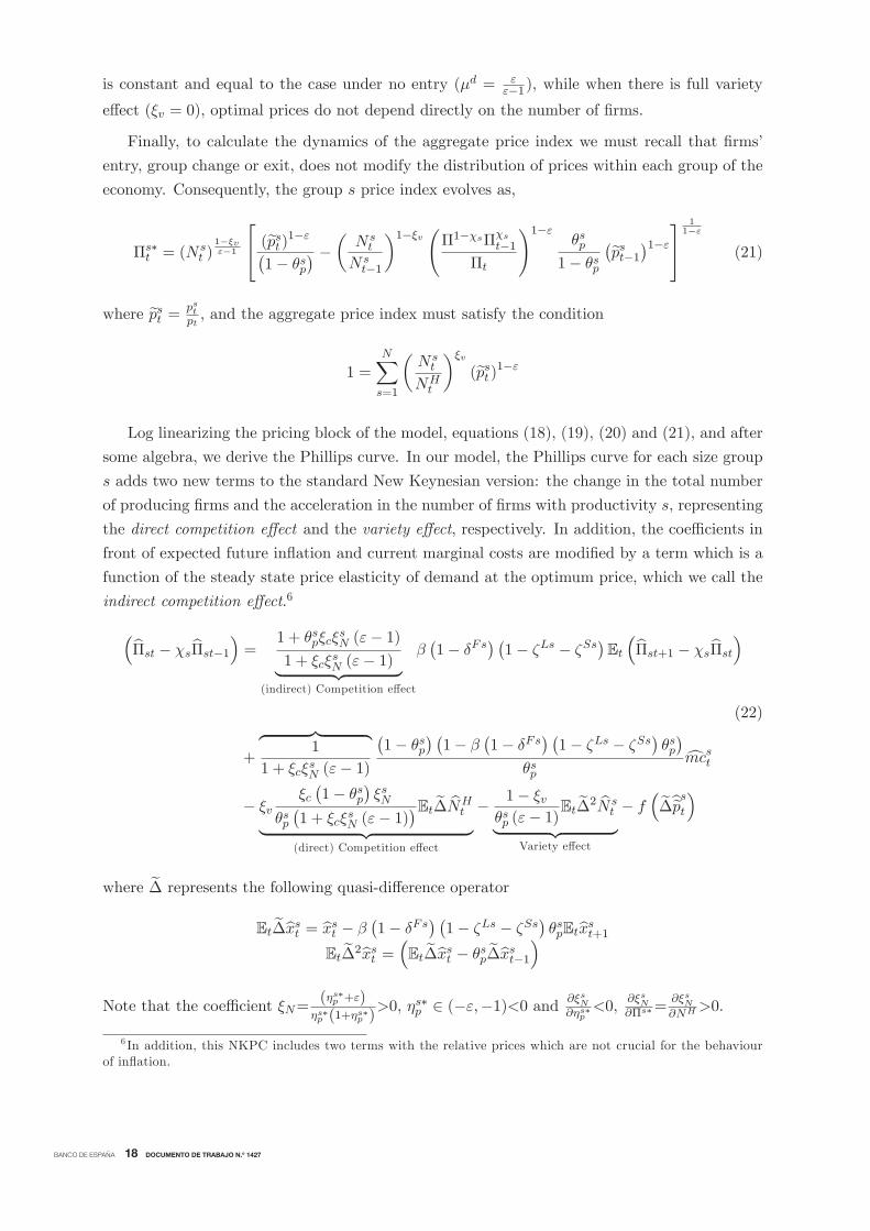
Log linearizing the pricing block of the model, equations (18), (19), (20) and (21), and after
some algebra, we derive the Phillips curve. In our model, the Phillips curve for each size group
s adds two new terms to the standard New Keynesian version: the change in the total number
of producing firms and the acceleration in the number of firms with productivity s, representing
the direct competition effect and the variety effect, respectively. In addition, the coefficients in
front of expected future inflation and current marginal costs are modified by a term which is a
function of the steady state price elasticity of demand at the optimum price, which we call the
indirect competition effect.6
Πst − χsΠst−1 =1 + θspξcξ
sN (ε− 1)
1 + ξcξsN (ε− 1)(indirect) Competition effect
β 1− δFs 1− ζLs − ζSs Et Πst+1 − χsΠst
(22)
+1
1 + ξcξsN (ε− 1)1− θsp 1− β 1− δFs 1− ζLs − ζSs θsp
θspmcst
− ξvξc 1− θsp ξsN
θsp 1 + ξcξsN (ε− 1)EtΔNH
t
(direct) Competition effect
− 1− ξvθsp (ε− 1)
EtΔ2N st
Variety effect
− f Δps
t
where Δ represents the following quasi-difference operator
EtΔxst = xst − β 1− δFs 1− ζLs − ζSs θspEtxst+1EtΔ2xst = EtΔxst − θspΔx
st−1
Note that the coefficient ξN=(ηs∗p +ε)
ηs∗p (1+ηs∗p )>0, ηs∗p ∈ (−ε,−1)<0 and ∂ξsN
∂ηs∗p<0, ∂ξsN
∂Πs∗=∂ξsN∂NH>0.
6 In addition, this NKPC includes two terms with the relative prices which are not crucial for the behaviourof inflation.
is constant and equal to the case under no entry (μd = εε−1), while when there is full variety

BANCO DE ESPAÑA 19 DOCUMENTO DE TRABAJO N.º 1427
Finally, aggregating across all sizes we get the aggregate NKPC
Πt =
N
s=1
N s (Πs∗)1−ε
(NH)ξvΠst +
ξv(1− ε)
Δ N st −NH
t .
Aggregate inflation is a weighted average of the inflation rates across size groups, and the change
in the shares of firms of each type , where the weights are inversely proportional to the steady
state optimal relative price. These equations are discussed at length at the beginning of the
results section.
2.3.3 Aggregate Constraints
Finally, to close the model, we derive the economy wide constraint using the aggregate household
budget constraint and the equilibrium conditions in the labor and goods markets:
(ct + it) (vpt )−ε+NEt vt
mcEt= At
kt−1ldt
α
ldt (23)
where aggregate price dispersion is defined as (vpt )−ε= 1
(NHt )
ξv
NHt
i=0pitpt
−ε, and, using the
properties of the index under Calvo’s pricing, evolves as,
(vpt )−ε= NH
t1−ξv
(1− θp)Π∗−εt +
NHt
NHt−1
1−ξvθp
Π1−χΠχt−1
Πt
−εvpt−1
−ε. (24)
and the average profit:
dFt =ct + it
NHt
1−mcHt (vpt )−ε (25)
As regards monetary policy we assume that the central bank sets the nominal interest rates
according to the following Taylor rule,
RtR=
Rt−1R
γR ΠtΠ
γΠ ydtyd
γy 1−γRexp (mt) (26)
Where Π represents the target level of inflation (equal to inflation in the steady state), R the
steady state nominal gross return on capital and mt is a random shock to monetary policy
that follows mt = σmεmt, where εmt is distributed according to N (0, 1). The presence of theprevious period interest rate, Rt−1, is justified because we want to match the smooth profile ofthe interest rate over time observed in the data.7
7Note that R is beyond the control of the monetary authority, since it is equal to the steady state real grossreturns of capital plus the target level of inflation.

BANCO DE ESPAÑA 20 DOCUMENTO DE TRABAJO N.º 1427
2.4 Calibration
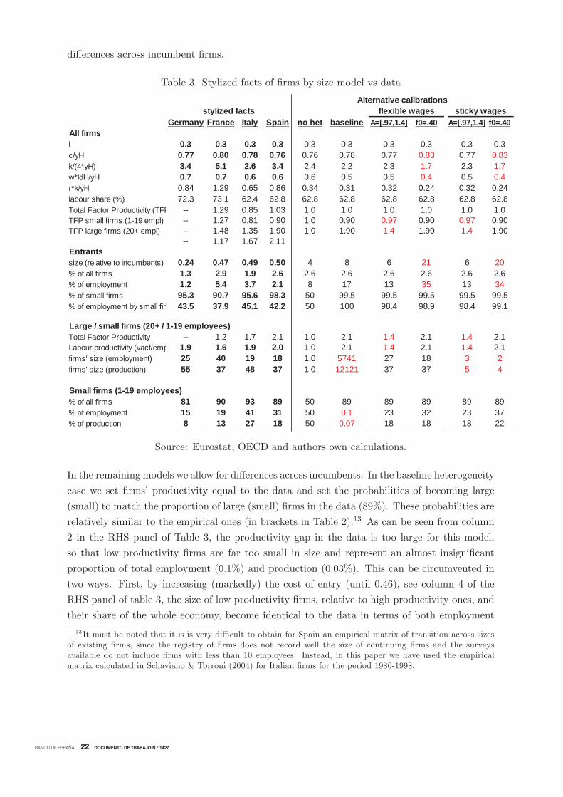
The model has 24 calibrated parameters, shown in Table 2. The first two columns display the
14 parameters that determine the steady state solution, the others affecting only the model
dynamics. These parameters have been calibrated either using consensus values taken from the
literature or were chosen to reproduce some data moments. In particular, we aim at approxi-
mating the stylized facts of the industrial structure,as well as the main macroeconomic ratios
of the Spanish economy, in bold in the fourth column of Table 3.8 The first block of these
(top block in bold) refers to long run (steady-state) ratios of the whole economy, the second
one refers to characteristics of entrant firms, while the last two blocks refer to characteristics of
large and small firms.
Table 2. Baseline Calibration
steady state parameters dynamics parameters
β = 0.99 ε = εw = 15
ϑ = σ = A =1 αH = 0.372
ϕ = 10 αE = 0
δ = δF = 0.025 fE = 0.11
AL = 1.9 ζL = 0.5% (0.2)
AS = 0.9 ζS = 1.5% (2.6)
κ = 0.1 γy = 0.125
χ = χw = 0.125 ρA = 0.7
θp = θw = 0.896 ρm = 0
γR = 0.8 ρd = 0.9
γπ = 1.7 ρmu = 0.7
First, it is worth noting that a model of firm entry with capital poses problems for determinacy
and non-explosiveness of the solution, as there might be now increasing returns to an accumu-
lated factor, physical capital. This is exacerbated when a complete variety effect is assumed.
Therefore, in this model, a unique, non-explosive solution cannot be guaranteed for a wide range
of standard parameter values. This problem can be circumvented in several ways. One may set
the parameters determining the steady state so as to reduce the increasing returns to capital,
for example, by assuming very fast physical capital depreciation, around 50% per quarter (like
in Bilbiie et al., 2008) or Lewis and Poilly, 2009), or through other parameters, mainly ϑ, ε and
ϕ. Alternatively, as it is done in this paper, one may assume that new entrants do not need
capital to produce (see Bilbiie et al., 2012). This approach allows for a wider parameter space,
however, it is still more reduced than when there is no capital accumulation.
We start by setting the parameters that affect only the dynamics of the model (right panel
of Table 2). The parameters of the Taylor rule are set to the standard estimation results for the
euro area (Clarida, Galí, and Gertler, 2000). On the nominal side, the Calvo and the indexation
to inflation parameters for prices and wages are similar to the values generally obtained for the
euro area (Smets and Wouters, 2005), while a very small adjustment cost for investment (κ) is
assumed.8Although the theoretical model and the simulation code admit any finite number of productivity classes, for
expository purposes we will carry out the empirical exercises below considering the simplest case of just two typesof firms: low productivity or small (S) and high productivity or large (L).

BANCO DE ESPAÑA 21 DOCUMENTO DE TRABAJO N.º 1427
Then we set the parameters that affect mainly the whole-economy steady state ratios and
the characteristics of entrants. The discount factor β is set to be consistent with an annualized
real interest rate of 2.5 percent and an inflation objective of 2 percent, so that the steady state
annual nominal interest rate (R) is 4.5 percent. The depreciation rate of capital is consistent
with an annual depreciation of 10%. The calibration of utility parameters is quite standard, with
log utility of consumption (σ = 1). The Frisch elasticity of labor supply is 1 (1/ϑ) in line with
the findings of the recent microeconomics literature (Browning, Hansen, and Heckman, 1999).9
The labor supply coefficient is set to 10, in line with estimated DSGE models (Fernández-
Villaverde, 2009).10 The elasticity of substitution between different types of intermediate goods
produced (ε) and between different labour types (εw) is slightly higher than what is normally
used in DSGE models, implying a lower mark-up of around 7 percent.11 The labour share of
incumbents is set equal to the value in the data for Spain, while the one of entrants is set to
1. Finally, the firms’ death rate δF is such that 10 percent of annual production is destroyed,
both as a share of products and as market share (Bilbiie et al., 2012, and Bernard et al., 2010).
The entry cost fE is one of the main determinants of the characteristics of entrant firms. A
low level of this parameter, 0.11, guarantees that entrant firms represent in steady state a small
share of firms and of production, similar to the data (2.5%). However entrant firms in this
model are much larger in terms of employment (4 times the size of an average incumbent) than
in the data (50%). This failure to replicate the data is mainly a consequence of the fact that
to increase the parameter space we have assumed that entrants are more labour intensive than
incumbents, with a markedly lower labour productivity.
The last set of parameters determine the differences across incumbent firms. First of all, we
consider a model without heterogeneity across firms, thus, these parameters are set equal. The
probabilities of firms becoming large (ζL = 52%) or small (ζS = 49%) are set so that 50% of
firms belong to each group and they represent 50% of employment and production, while firms’
productivity (AL, AS) is set to the average (1). The result of this calibration is reported in the
first column of the right hand side panel of Table 312. This calibration delivers model steady
state ratios for the share of consumption in final demand, the labour share and the capital to
GDP ratio which are fairly close to the ones in the data, while entrant firms characteristics are
well approximated, except for their size. However, by definition is unable of generating any
9 If we assumed higher values, as normally done in macro models (lower ϑ), the steady state level of labourwould be too low.10The model cannot be solved for lower values, however these would not help to approximate better the steady
state ratios.11Again, the model cannot be solved for lower values, but even if we could it would not help to match the
size of entrants. This is another consequence of the somehow smaller parameter space in this model due to theincreasing returns to capital.12Note that we do not report separately the relevant steady state ratios for the model with and without variety
effect, since they are very similar.
BANCO DE ESPAÑA 22 DOCUMENTO DE TRABAJO N.º 1427
differences across incumbent firms.
Table 3. Stylized facts of firms by size model vs data
Germany France Italy Spain no het baseline A=[.97,1.4] f0=.40 A=[.97,1.4] f0=.40All firmsl 0.3 0.3 0.3 0.3 0.3 0.3 0.3 0.3 0.3 0.3c/yH 0.77 0.80 0.78 0.76 0.76 0.78 0.77 0.83 0.77 0.83k/(4*yH) 3.4 5.1 2.6 3.4 2.4 2.2 2.3 1.7 2.3 1.7w*ldH/yH 0.7 0.7 0.6 0.6 0.6 0.5 0.5 0.4 0.5 0.4r*k/yH 0.84 1.29 0.65 0.86 0.34 0.31 0.32 0.24 0.32 0.24labour share (%) 72.3 73.1 62.4 62.8 62.8 62.8 62.8 62.8 62.8 62.8Total Factor Productivity (TFP -- 1.29 0.85 1.03 1.0 1.0 1.0 1.0 1.0 1.0TFP small firms (1-19 empl) -- 1.27 0.81 0.90 1.0 0.90 0.97 0.90 0.97 0.90TFP large firms (20+ empl) -- 1.48 1.35 1.90 1.0 1.90 1.4 1.90 1.4 1.90
-- 1.17 1.67 2.11Entrantssize (relative to incumbents) 0.24 0.47 0.49 0.50 4 8 6 21 6 20% of all firms 1.3 2.9 1.9 2.6 2.6 2.6 2.6 2.6 2.6 2.6% of employment 1.2 5.4 3.7 2.1 8 17 13 35 13 34% of small firms 95.3 90.7 95.6 98.3 50 99.5 99.5 99.5 99.5 99.5% of employment by small fir 43.5 37.9 45.1 42.2 50 100 98.4 98.9 98.4 99.1
Large / small firms (20+ / 1-19 employees)Total Factor Productivity -- 1.2 1.7 2.1 1.0 2.1 1.4 2.1 1.4 2.1Labour productivity (vacf/emp 1.9 1.6 1.9 2.0 1.0 2.1 1.4 2.1 1.4 2.1firms' size (employment) 25 40 19 18 1.0 5741 27 18 3 2firms' size (production) 55 37 48 37 1.0 12121 37 37 5 4
Small firms (1-19 employees)% of all firms 81 90 93 89 50 89 89 89 89 89% of employment 15 19 41 31 50 0.1 23 32 23 37% of production 8 13 27 18 50 0.07 18 18 18 22
stylized facts sticky wagesAlternative calibrations
flexible wages
Source: Eurostat, OECD and authors own calculations.
In the remaining models we allow for differences across incumbents. In the baseline heterogeneity
case we set firms’ productivity equal to the data and set the probabilities of becoming large
(small) to match the proportion of large (small) firms in the data (89%). These probabilities are
relatively similar to the empirical ones (in brackets in Table 2).13 As can be seen from column
2 in the RHS panel of Table 3, the productivity gap in the data is too large for this model,
so that low productivity firms are far too small in size and represent an almost insignificant
proportion of total employment (0.1%) and production (0.03%). This can be circumvented in
two ways. First, by increasing (markedly) the cost of entry (until 0.46), see column 4 of the
RHS panel of table 3, the size of low productivity firms, relative to high productivity ones, and
their share of the whole economy, become identical to the data in terms of both employment
13 It must be noted that it is is very difficult to obtain for Spain an empirical matrix of transition across sizesof existing firms, since the registry of firms does not record well the size of continuing firms and the surveysavailable do not include firms with less than 10 employees. Instead, in this paper we have used the empiricalmatrix calculated in Schaviano & Torroni (2004) for Italian firms for the period 1986-1998.

BANCO DE ESPAÑA 23 DOCUMENTO DE TRABAJO N.º 1427
and production . However, in this case entrant firms have to be much larger (22 times the
incumbents’ size) to cover for the sunk cost of entry and therefore represent an unrealistic share
of total employment and production. Moreover, this calibration also produces unrealistic values
for most whole economy steady state ratios, like too high a consumption share of final demand or
too low a capital and labour rents’ share of GDP. Secondly, and more promising, one can reduce
the productivity gap, while keeping the average constant. In particular, as shown in column 3
of the RHS panel of Table 3, if the productivity gap is reduced from 2.1 to 1.4, the model is able
to match fairly well the data on the size of low productivity firms and their share of the whole
economy in terms of production, and to a less extent in terms of employment. Moreover, this
is achieved while matching slightly better than the baseline case the characteristics of entrants
and without worsening the whole economy steady state ratios.
Finally, when we add sticky wages to the model (of a similar magnitude of price stickiness),
in the last two columns of table 3, most of the steady state ratios are unchanged, except that
now firms’ size is smaller than in the data, due to the fact that this assumption rises steady
state wages, since it adds a mark up to them, increasing the costs to setup firms and reducing
their size.
3 Steady state analysis
In this section we analyze the steady state effect of changes in some of the more relevant
parameters of the model that may be relevant for policy analysis. Table 4 shows the (sign of
the) impact of changes in ε, εw, ϑ, ψ, δ, αH , A, AE , fE and δF on the most important variables
and ratios of the three models considered: a model with entry, with entry and firm heterogeneity
(in size) and without entry.
First of all, we look at the parameters not related directly to firms’ entry, included in the
first three blocks of the table. The impact of changes in these parameters (ϑ, ψ, σ, εw, A) is
qualitatively identical and quantitatively similar across the models considered. In particular,
a decrease in the disutility of labor (either through a greater inverse of the Frisch elasticity ϑ
or a larger weight of the labour component in the utility function ψ), a rise in the utility from
consumption (σ) or the elasticity of substitution amongst labour types (εw) all increase the
willingness of households to work, which rises firms’ production and total GDP, while a rise in
the average TFP level (A) rises firms’ production and GDP directly. In the models with entry
and size, this in turn, improves the value of future entrants, and incentivizes the entry of new
firms.
The exception to this is the elasticity of substitution across consumption varieties (ε) (see
fourth panel of table 4). In a model with no entry, a rise in ε implies an increase in competition
amongst firms through a fall in the steady state markup, which reduces firms’ profits. Therefore,
they react by moving along their demand schedules increasing production and employment, that
in turn rises wages and consumption. This is the reason why this parameter is often used as

BANCO DE ESPAÑA 24 DOCUMENTO DE TRABAJO N.º 1427
a proxy for structural reforms in the goods market in a model without entry. However, when
one also considers the possibility of firms entry, there are other relevant developments in the
economy. In a model with entry, a lower markup initially reduces profits per firm. Thus, a
smaller number of firms enter the market until expected profits per producing firm are restored
to their original value, when each incumbent produces more, with more capital and labor.
In addition, the smaller number of firms reduces competition and partially offsets the fall in
markups. Despite this, aggregate output, consumption and employment in the production
sector increase by more in the case with entry. On the contrary, in the model with entry and
size heterogeneity, the rise in ε reduces the markup of small/low productivity firms (−0.7%) bytwice as much as the one of large/more productive firms (−0.3%). This leads to a rise (fall) inemployment, capital and production of larger (smaller) firms and of the aggregate, which leads
to an increase in total entry, since entrants expect to become large eventually. The reason for
this is that large firms, thanks to their technological advantage, face a more inelastic segment
of the demand curve, which allows them to lower their optimal relative prices by less than small
firms.
Table 4. Impact on the steady state of changes in parameters
In a model where consumers derive greater utility from a larger number of varieties of goods
(variety effect), there is another balancing effect. If consumers value varieties a lot, the reduction
in the number of entrants has a negative effect on consumption, which compensates the positive
one coming from the lower markup and leaves aggregate production and employment unchanged,
although employment in production increases, while capital, investment and wages fall.
The last two columns of table 4 show the impact of a change in the distribution of produc-
tivity in the model with heterogeneity of an increase in the productivity of the largest firms
(column before last) and of a mean preserving increase in the dispersion of productivity (last

BANCO DE ESPAÑA 25 DOCUMENTO DE TRABAJO N.º 1427
column). The steady state impacts are qualitatively similar, with a rise in almost all aggregates,
except for employment, due to the reduction in small firms employment. This is even true in
the case of the mean preserving shock, since the positive impact of a rise in the productivity of
the largest firms dominates the negative one of reducing the productivity of the small firms.
One of the advantages of modelling firms’ entry is that now we have several parameters that
govern the entry process and affect directly the degree of competition in the economy, being
therefore much better proxies of structural reforms than the elasticity of substitution between
consumption varieties (ε). In particular, the relevant parameters are the cost of entry (fE) and
the technological level of entrants (AE), which jointly (together with the real wage) determine
the total cost of entry (fEmcE = fE wAE); and the the firms’ (exogenous) probability of death
(δF ), which determines the exit from the market.
A fall in fE and an improvement in entrants technology (AE), reduce the total cost of
entry (fEmcE = fE wAE), which increases the number of producing firms. On the other hand,
a fall in the producing firms’ death rate (δF ), also increases the number of surviving firms,
while reducing the incentive to enter and therefore the number of entrants. In all cases, this
augments the intensity of competition in the economy and lowers the markup and profits of each
existing firm. Therefore, the economy has a larger number of firms charging a lower markup,
which increases aggregate production and consumption. A side implication of the smaller cost
of entry or lower probability of death is that now firms do not need to be as big to afford entry,
so in equilibrium they become smaller, both in terms of production and employment.
Table 5. Impact on the mark up of changes in parameters
Table 5 compares the quantitative impact on consumption and the number of firms of a change
in these parameters that reduces the markup by 0.1 percentage points. Starting with the case of
the model with entry but no variety effect (column 2 in the table), firstly, note that the required

BANCO DE ESPAÑA 26 DOCUMENTO DE TRABAJO N.º 1427
percentage change in these parameters to achieve that fall in the markup is around 7-11%,
instead of the 1% increase in ε. Secondly, the impact on consumption and output is similar to
the baseline for the parameters changing the entry cost, but it doubles for the fall in the death
rate. Thirdly, the number of producing (and entrant) firms increases by more than six percent,
in contrast with the 1% reduction in the baseline. This is consistent with the different ways of
achieving stronger competition through changes in ε vis a vis changes in fE or AE ; whereas in
the former case the reduction in the market power is the cause of a fall in expected profits that
discourages entry, in the latter, each firms’ market power falls as more firms are willing to enter
due to the lower entry costs. The same logic applies to the reduction (by 3.6%) in the number
of entrants when the death rate falls; since the number of producing firms increases, the level of
expected profits critical for the entry decision goes down. In the case of the model with variety
effect (column 3 in the table), the impact on consumption and output is around eight and four
times greater than in the baseline, respectively. This reflects the fact that consumers value the
number of varieties in the economy, which reduces the cost of achieving a given level of utility.
Finally, when we allow for size heterogeneity we find a much stronger impact on output and
consumption (5 and 7 times) and a weaker impact on entry (a half).
4 Results: Firm entry and inflation
In the rest of the paper we investigate the effect of entry and firm heterogeneity on the response
of the main macroeconomic variables to different shocks. In particular we first focus on the
dynamics of inflation conditional on productivity shocks to describe in detail the mechanism
that drives apart the response of this variable with respect to what would occur in a model
with a fixed number of productive firms. We then extend our analysis to the responses of other
shocks. Key to understanding the differences with the standard non-entry model is expression
(22); given the complexity of the mechanisms involved we carry out this analysis in two steps.
First we compare the model with homogeneous firms with that of no entry and then in the next
section we shall focus on the heterogeneity issue.
The New Keynesian Phillips curve in the model with homogenous firms (Ast = At ∀s) is aparticular case of (22) that now becomes:
Πt − χΠt−1 =1 + ξcξNθp (ε− 1)1 + ξcξN (ε− 1)
(indirect) Competition effect
β 1− δF Et Πt+1 − χΠt (27)
+1
1 + ξcξN (ε− 1)(1− θp) 1− β 1− δF θp
θpmct
− ξvξcξN (1− θp)
θp (1 + ξcξN (ε− 1))EtΔNHt
(direct) Competition effect
− 1− ξvθp (ε− 1)EtΔ
2NHt
Variety effect
BANCO DE ESPAÑA 27 DOCUMENTO DE TRABAJO N.º 1427
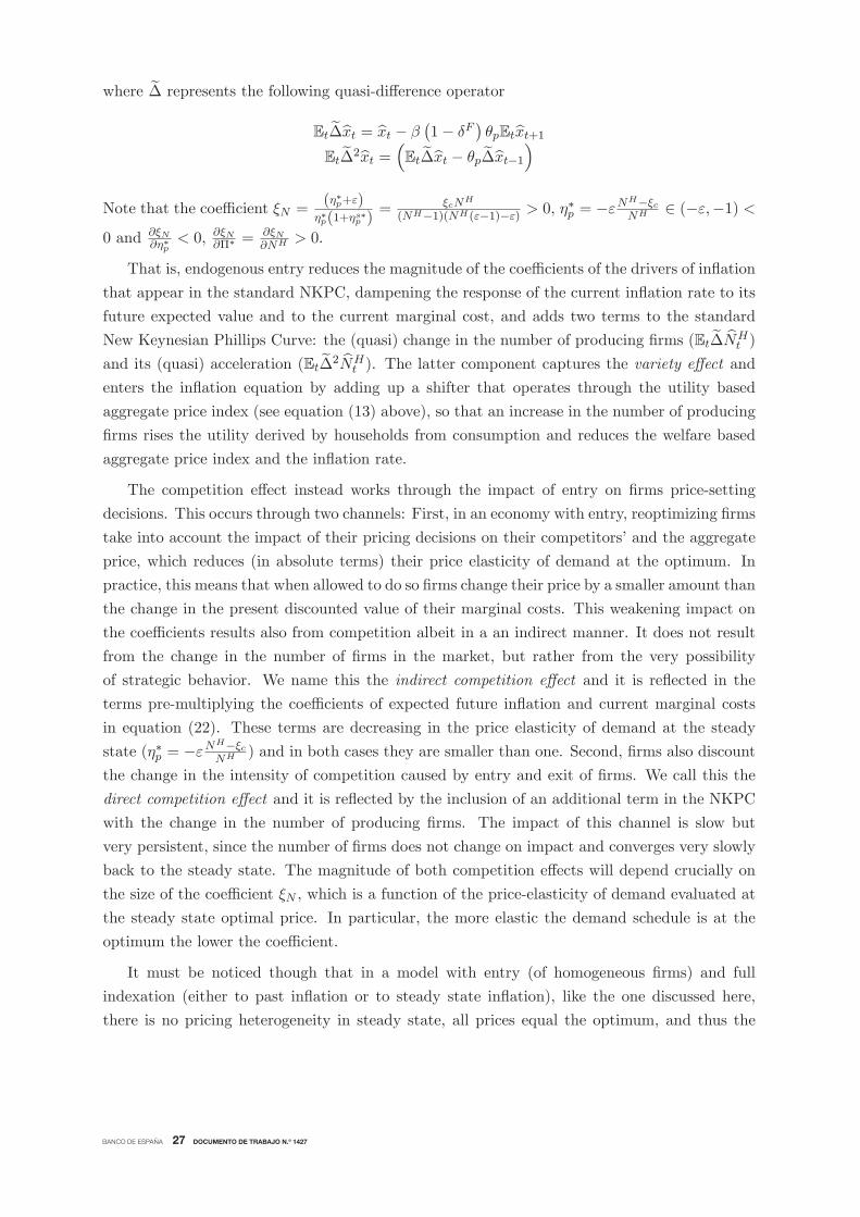
where Δ represents the following quasi-difference operator
EtΔxt = xt − β 1− δF θpEtxt+1EtΔ2xt = EtΔxt − θpΔxt−1
Note that the coefficient ξN =(η∗p+ε)
η∗p(1+ηs∗p )= ξcNH
(NH−1)(NH(ε−1)−ε) > 0, η∗p = −εN
H−ξcNH ∈ (−ε,−1) <
0 and ∂ξN∂η∗p
< 0, ∂ξN∂Π∗ =
∂ξN∂NH > 0.
That is, endogenous entry reduces the magnitude of the coefficients of the drivers of inflation
that appear in the standard NKPC, dampening the response of the current inflation rate to its
future expected value and to the current marginal cost, and adds two terms to the standard
New Keynesian Phillips Curve: the (quasi) change in the number of producing firms (EtΔNHt )
and its (quasi) acceleration (EtΔ2NHt ). The latter component captures the variety effect and
enters the inflation equation by adding up a shifter that operates through the utility based
aggregate price index (see equation (13) above), so that an increase in the number of producing
firms rises the utility derived by households from consumption and reduces the welfare based
aggregate price index and the inflation rate.
The competition effect instead works through the impact of entry on firms price-setting
decisions. This occurs through two channels: First, in an economy with entry, reoptimizing firms
take into account the impact of their pricing decisions on their competitors’ and the aggregate
price, which reduces (in absolute terms) their price elasticity of demand at the optimum. In
practice, this means that when allowed to do so firms change their price by a smaller amount than
the change in the present discounted value of their marginal costs. This weakening impact on
the coefficients results also from competition albeit in a an indirect manner. It does not result
from the change in the number of firms in the market, but rather from the very possibility
of strategic behavior. We name this the indirect competition effect and it is reflected in the
terms pre-multiplying the coefficients of expected future inflation and current marginal costs
in equation (22). These terms are decreasing in the price elasticity of demand at the steady
state (η∗p = −εNH−ξcNH ) and in both cases they are smaller than one. Second, firms also discount
the change in the intensity of competition caused by entry and exit of firms. We call this the
direct competition effect and it is reflected by the inclusion of an additional term in the NKPC
with the change in the number of producing firms. The impact of this channel is slow but
very persistent, since the number of firms does not change on impact and converges very slowly
back to the steady state. The magnitude of both competition effects will depend crucially on
the size of the coefficient ξN , which is a function of the price-elasticity of demand evaluated at
the steady state optimal price. In particular, the more elastic the demand schedule is at the
optimum the lower the coefficient.
It must be noticed though that in a model with entry (of homogeneous firms) and full
indexation (either to past inflation or to steady state inflation), like the one discussed here,
there is no pricing heterogeneity in steady state, all prices equal the optimum, and thus the

BANCO DE ESPAÑA 28 DOCUMENTO DE TRABAJO N.º 1427
competition effect is likely to be very small. Table 6, reports the values of the coefficients in both
versions of the NKPC above for our baseline calibration. When there is entry, the (indirect)
competition effect lowers the coefficients of future inflation and current marginal costs around
6%, while the coefficient of the change in the number of firms is very small in magnitude (-.003).
The opposite is true for the variety effect, whose (negative) coefficient is greater than the one
of marginal costs. However, since the dynamics of the number of firms is very persistent, its
acceleration will not move very much, except just after the initial impact.
Table 6. Parameters of New Keynesian Phillips Curve (equation (27))
EtΠt+1 mct EtΔNHt EtΔ2NH
t
no entry .990 .086 0 0
entry .933 .080 −.003 0
variety .933 .080 0 .095
Finally, notice that if we shut down the competition and the variety effects (ξc = 0, ξv = 1),
this expression boils down to the standard non-entry NKPC with a discount rate augmented
by the survival rate of firms (1− δF ).
At this stage it might be worth comparing the Phillips curve derived from our model with
the one obtained previously by other researchers in models with entry. Differences among (27)
and the price equations obtained by other authors in models with entry stem from two sources:
first, our assumption of Calvo pricing, which departs from the Rotemberg costly price setting
framework in Bilbiie et al (2008) and Lewis & Poilly (2012); and second, other assumptions re-
garding the industry structure. In terms of our notation the equivalent NKPC under Rotemberg
pricing would take the following form14
Πt − χΠt−1 = β 1− δF EtΠt+1 − χΠt +η∗p − 1
κmct
(indirect) Competition effect
− ξcε
η∗pNHκNHt
(direct) Competition effect
− (1− ξv)1
κNHt −
1
ε− 1 ΔNHt − β 1− δF ΔEtNH
t+1
Variety effect
where κ is the Rotemberg parameter of price rigidities and Δ is the difference operator. This
expression has similar ingredients to the one under Calvo setting, except that in this case the
indirect competition effect only changes the slope of the NKPC (marginal cost coefficient),
since η∗p is a (negative) function of the number of firms in the economy, but not the forwardlooking component. In addition, the direct competition effect in this case does not include a
14 In deriving this expression we have imposed the same assumptions as in the rest of the paper, namely, avariable variety effect and a standard utility function. Alternatively, if we assumed a Feenstra utility functionaccording to which consumers derive utility from increasing the number of varieties, the coefficient in front of
NHt would be η + 1−ξv
ε−1ε−1κ, where η is the elasticity of the desired mark up to the number of varieties in the
utility.

BANCO DE ESPAÑA 29 DOCUMENTO DE TRABAJO N.º 1427
forward looking component of the change in the number of firms. Bilbiie et al. (2008) price
equation is similar to this expression but assuming no competition effect (ξc = 0 and η∗p = −ε),
and concentrating on the variety effect. On the other hand, Lewis and Poilly (2012) extend
this expression to include the supply structure proposed by Jaimovich and Floetotto (2008),
where there is a continuum of industries with firm entry. The main difference with the equation
derived above is that in their case the steady state price elasticity of demand is a function of
the difference between the within (ε) and the between (εI) industries’ elasticity of substitution,
η∗p = ε− (ε− εI)1NH .
4.1 Productivity shocks
In Figure 2 we depict the impulse responses of the main aggregate variables to a positive shock
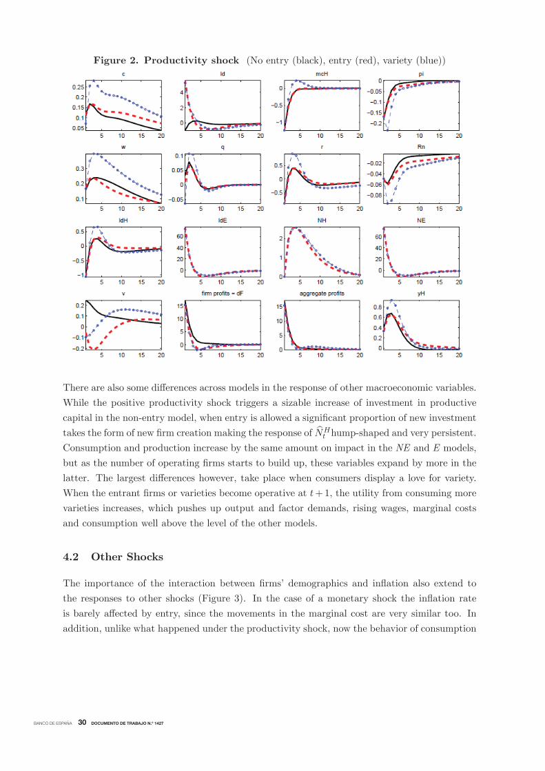
to total factor productivity. We start by discussing the differential response of the inflation rate
in the three models, no entry (NE black continuous line) versus entry (E, red dashed line) and
entry cum variety effect (EV, blue dotted line), all of them featuring firm homogeneity. While
the NE and the E models display different responses in several macroeconomic variables, there
are small differences in the dynamics of inflation: The inflation rate falls sharply on impact by
the same amount in both cases but the subsequent return towards equilibrium is slightly more
persistent in the entry model, in which the adjustment is not complete after 20 periods while in
the non-entry case the adjustment is almost complete after 10 periods. This difference reflects
the small but very persistent impact of the number of producing firms (direct competition effect)
on inflation. The entry of new firms is triggered by the fall in marginal costs that increases firm
profits. The number of hours worked by new entrants rises sharply although new firms become
productive with a lag and display an inverted U-shape with great persistence.15
The dynamic response in the variety (V ) model is significantly different at t = 1. Although
the inflation rate falls on impact by a similar magnitude as in the non-entry and entry cases it
falls then further as the acceleration in the number of firms affects directly the CPI index.
15This similarity of the dynamics of inflation across the non-entry and entry models depends crucially onthe degree of stickiness of marginal costs, that is, of wages, which in our baseline calibration is fairly high. Inan economy with entry and flexible wages, marginal costs, and consequently inflation, fall on impact by muchless. The reason is that the dynamics of marginal costs are now driven by the fact that the productivity shocktriggers an entry of firms. Thus although the demand for labor in incumbent firms falls due to the presence pricestickiness, there is a new source of labor demand by entrants. This increase in labor demand comes along withan increase in wages that dampens the reduction in marginal costs.
BANCO DE ESPAÑA 30 DOCUMENTO DE TRABAJO N.º 1427
Figure 2. Productivity shock (No entry (black), entry (red), variety (blue))
There are also some differences across models in the response of other macroeconomic variables.
While the positive productivity shock triggers a sizable increase of investment in productive
capital in the non-entry model, when entry is allowed a significant proportion of new investment
takes the form of new firm creation making the response ofNHt hump-shaped and very persistent.
Consumption and production increase by the same amount on impact in the NE and E models,
but as the number of operating firms starts to build up, these variables expand by more in the
latter. The largest differences however, take place when consumers display a love for variety.
When the entrant firms or varieties become operative at t+1, the utility from consuming more
varieties increases, which pushes up output and factor demands, rising wages, marginal costs
and consumption well above the level of the other models.
4.2 Other Shocks
The importance of the interaction between firms’ demographics and inflation also extend to
the responses to other shocks (Figure 3). In the case of a monetary shock the inflation rate
is barely affected by entry, since the movements in the marginal cost are very similar too. In
addition, unlike what happened under the productivity shock, now the behavior of consumption

BANCO DE ESPAÑA 31 DOCUMENTO DE TRABAJO N.º 1427
is very similar across models. The reason is that the productivity shock hits the entry process
directly by reducing marginal costs and a substantial amount of resources is devoted to entry
and ’distracted’ from other uses. Here the opposite happens, with a fall in NE , which diminishes
the costs associated to the entry process.
Inflation displays somewhat more different patterns across entry models following other
types of shocks. The preference shock and the labor supply shocks, give rise to very different
inflation dynamics; in both cases the impact effect under no entry is the largest, but as the
number of operating firm diminishes, the inflation increases by more in the variety case. After
a positive preference shock that increases consumption and the real wage, the marginal costs
rises, reducing firm’s profits and the number of entrants; this in turn reduces the number of
active firms which means an additional push on inflation in the VE model long after the effects
of the rise in the marginal costs have vanished.
Not surprisingly the largest differences among the E and the VE models occur in response
to an entry cost shock. After this contractionary shock output and employment fall whereas
inflation rises. The‘positive response of inflation is most interesting since this occurs, unlike
any other type of shock, despite the fact that the marginal cost actually falls due to the sharp
drop in the number of entrants that reduces the number of operative units and wages. The rise
in fE reduces the incentive to enter in the market and hence the number of operating firms.
In the variety case this acts as a powerful inflationary mechanism that more than compensates
the fall in mct.
The results in this section indicate that the differences in conditional inflation dynamics
among models in which the number of firms remain constant along the cycle and those in
which there is entry and exit, rely on the strength of the variety effect. In other words, as the
theoretical model above suggests strategic pricing behavior and competition among incumbents
and potential entrants, that is very often pointed as a key driving force of inflation, plays a
minor role. Consequently, competitiveness seems to be disconnected from the barriers of entry
in the market. Important as it might be, the variety effect is not highly placed on the policy
agenda on this matter, nor is it straightforward to relate this concept with specific policy actions
to achieve more stable inflation rates. Admittedly, many of the discussions about policies to
foster competition and lower consumer prices include not only the entry/no entry dimension
but also look into another relevant feature of the market structure: heterogeneity of firms in
terms of productivity and size.

BANCO DE ESPAÑA 32 DOCUMENTO DE TRABAJO N.º 1427
Figure 3. Other shocks (No entry (black), entry (red), variety (blue))Monetary shock Labor supply shock
Preference shock Entry cost shock
5 Results: Heterogeneous firms and inflation
In order to further explore the importance of competition forces in the market we move on now
to study the implications of the presence of heterogeneous firms in the market. We conduct our

BANCO DE ESPAÑA 33 DOCUMENTO DE TRABAJO N.º 1427
analysis by comparing two versions of our general model, the standard entry model we have
discussed so far and a model with two types of firms: large (more productive) and small (less
productive). We then extend our exercise to consider a alternative industry structures in terms
of the dispersion of firms’ size and the number of firm types.
The NKPC for each group is similar to the case of homogeneous firms, except that now
all the parameters are group specific, while the (direct) competition effect refers to the total
number of producing firms,16
Πst − χsΠst−1 =1 + θspξcξ
sN (ε− 1)
1 + ξcξsN (ε− 1)(indirect) Competition effect
β 1− δFs 1− ζLs − ζSs Et Πst+1 − χsΠst
(28)
+1
1 + ξcξsN (ε− 1)1− θsp 1− β 1− δFs 1− ζLs − ζSs θsp
θspmcst
− ξvξc 1− θsp ξsN
θsp 1 + ξcξsN (ε− 1)EtΔNH
t
(direct) Competition effect
− 1− ξvθsp (ε− 1)
EtΔ2N st
Variety effect
− f Δps
t
where Δ represents the following quasi-difference operator
EtΔxst = xst − β 1− δFs 1− ζLs − ζSs θspEtxst+1EtΔ2xst = EtΔxst − θspΔx
st−1
Note that the coefficient ξN =(ηs∗p +ε)
ηs∗p (1+ηs∗p )> 0, ηs∗p = −ε 1− ξc N
H −ξv (Π∗s)1−ε , ηs∗p ∈
(−ε,−1) < 0 and ∂ξsN∂ηs∗p
< 0, ∂ξsN∂Πs∗ =
∂ξsN∂NH > 0.
This expression resembles the one in the homogeneous firms model, (27). However, in this
case the coefficient ξN may differ across productivity classes since the optimal relative price
is also very different among them due to the technological difference: higher than one in the
case of the smaller/less productive firms and lower than one for the larger/more productive
ones.17 Therefore, the price elasticity of demand is also very different across sizes: greater (in
absolute terms) in the case of small firms, close to the no entry value (−ε), while it is much
smaller for the more productive firms. This means that when allowed to change their prices
more productive firms do so by much less than the present discounted value of marginal costs,
while small firms behave more like the case of homogeneous firms. As a consequence, both the
indirect competition effect (which is a negative function of the optimal relative price in steady
state (Πs∗)) and the direct competition effect (positive function of Πs∗) are much stronger in16 In addition, this NKPC includes two terms with the relative prices which are not crucial for the behaviour
of inflation.17 In a model with more than two types, those with productivity above (below) the average will set their optimal
prices in steady state at a level below (above) the average and their relative price will be below (above) one.
BANCO DE ESPAÑA 34 DOCUMENTO DE TRABAJO N.º 1427
the case of the more productive firms. That is, the coefficients in front of future inflation and
current marginal costs are smaller in the case of the more productive firms, while the one in
front of the change in the number of productive firms is greater.
Πt =
N
s=1
N s (Πs∗)−(ε−1)Ns=1N
s (Πs∗)1−εΠst − ξv
ε− 1Δ N st −NH
t (29)
Πt =
N
s=1
N s (Πs∗)1−εNs=1N
s (Πs∗)1−ε
⎡⎣Πst − ξv(ε− 1)
1
NH
N
r=s=1
1− (Πr∗)1−ε
(Πs∗)1−εΔN s
t
⎤⎦On the other hand, aggregate inflation is a weighted average of the inflation rate and the
change in the share of producing firms of each firm-size, where the weights are the share of
firms of each size in steady state times the inverse of their optimal relative price. As shown in
(29) this can be re-written in terms of the change in the number of firms of each productivity
level, times the difference in optimal relative prices. Given that the optimal relative price of
large (small) firms is smaller (greater) than one, this expression puts a much larger weight on
the inflation rate of the most productive firms, which will tend to dominate aggregate inflation
dynamics. With respect to the change in the number of producing firms of each size, in the
case of two sizes, the weights are identical but with different sign (positive for small, negative
for large firms). This represents the fact that small firms set a higher price, thus a rise in their
share of all firms increases aggregate inflation.
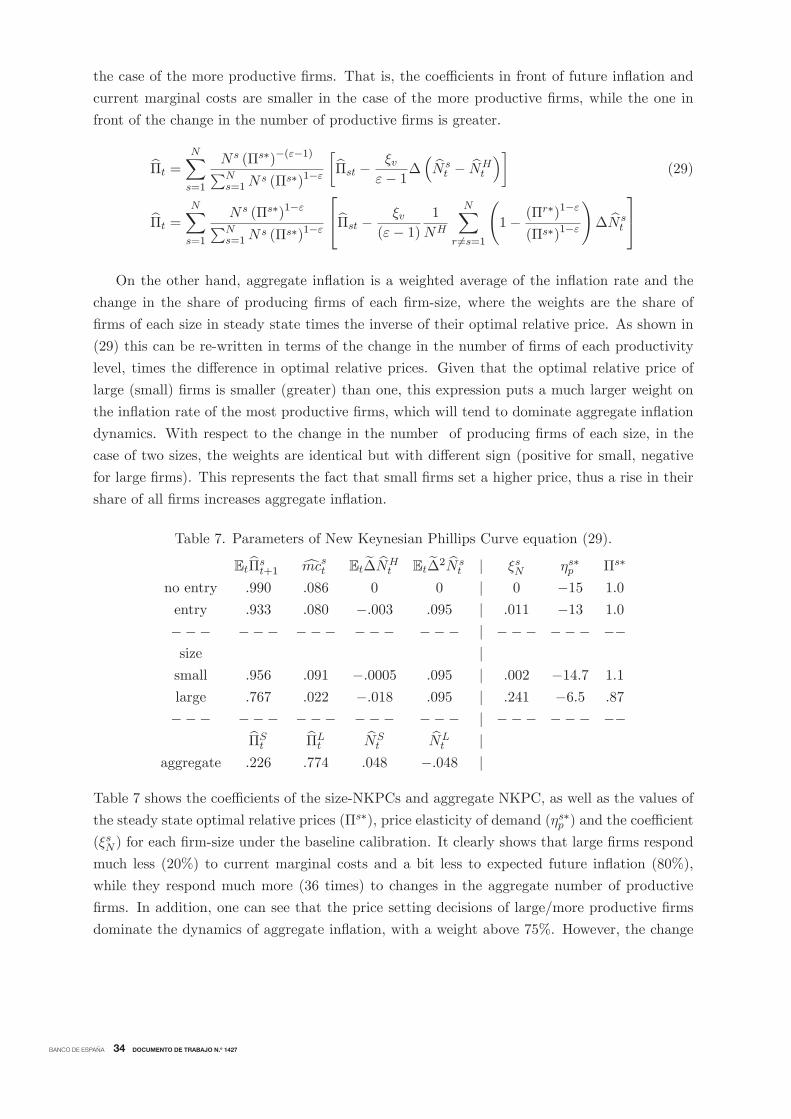
Table 7. Parameters of New Keynesian Phillips Curve equation (29).
EtΠst+1 mcst EtΔNHt EtΔ2N s
t | ξsN ηs∗p Πs∗
no entry .990 .086 0 0 | 0 −15 1.0
entry .933 .080 −.003 .095 | .011 −13 1.0
−−− −−− −−− −−− −−− | −−− −−− −−size |small .956 .091 −.0005 .095 | .002 −14.7 1.1
large .767 .022 −.018 .095 | .241 −6.5 .87
−−− −−− −−− −−− −−− | −−− −−− −−ΠSt ΠLt NS
t NLt |
aggregate .226 .774 .048 −.048 |
Table 7 shows the coefficients of the size-NKPCs and aggregate NKPC, as well as the values of
the steady state optimal relative prices (Πs∗), price elasticity of demand (ηs∗p ) and the coefficient(ξsN ) for each firm-size under the baseline calibration. It clearly shows that large firms respond
much less (20%) to current marginal costs and a bit less to expected future inflation (80%),
while they respond much more (36 times) to changes in the aggregate number of productive
firms. In addition, one can see that the price setting decisions of large/more productive firms
dominate the dynamics of aggregate inflation, with a weight above 75%. However, the change

BANCO DE ESPAÑA 35 DOCUMENTO DE TRABAJO N.º 1427
in the number of small firms will also have a strong impact on aggregate inflation since they
impact with the same magnitude but they represent a larger proportion of all firms.
We depict in Figures 4, 5 and 6 the impulse responses of the model with entry and ho-
mogeneous firms (E model, blue dotted lines) and those corresponding to the model with
heterogenous firms (S model, red dashed lines). The latter model allows for entry and exit of
firms but also for upgrading and downgrading in the level of productivity and size. To highlight
the importance of the competition effect in both worlds we abstract from the variety effect
throughout the exercise (the results are available from the authors upon request). In addition,
in figures 4 and 5 we also display the differential response of variables corresponding to small
and large firms.
As was mentioned above, it is worth noting that we are the first to derive the NKPC in
an economy with entry and size distribution. Lewis and Poilly (2012) derive the NKPC in an
economy with entry into different industries, but their objective is to analyze the impact of the
different degree of substitutability of goods within and between industries and thus they do not
consider size or productivity differences. In their case the steady state price elasticity of demand
is a function of the difference between the within (ε) and the between (εI) industries’ elasticity
of substitution, η∗p = ε − (ε− εI)1NH . Note that in their model, when these two elasticities of
substitution are identical we are back at the case without competition effect (η∗p = ε = εI), in
which the price elasticity of demand is constant and independent of the number of producing
firms. This is due to the fact that they assume that firms take into account the impact of a
change in their prices on the industry price, but not on the aggregate price.
5.1 Productivity shock
Regarding productivity shocks, the model with large and small firms displays a significantly
weaker reaction of the inflation rate than the model with homogeneous firms, despite the fact
that marginal costs fall by more and entry of new firms is stronger in the heterogeneity case.
The reasons behind this discrepancy have to do with the different behavior of small versus large
firms’ inflation as well as with the composition effect behind the aggregate rate. First, notice
that the impulse response function of the rate of inflation of small firms basically mimics the
response of inflation in the case of homogeneous firms (figure 4, panels A and B). The aggregate
behaves differently though due to the combination of two effects. First, large firms adjust their
prices significantly less on impact, because, as explained above, the strength of both the direct
and indirect competition effects disconnects to some extent the response of prices from the
dynamics of the marginal cost.

BANCO DE ESPAÑA 36 DOCUMENTO DE TRABAJO N.º 1427
Figure 4. Neutral Productivity shock
A) Aggregate responses: heterogenous (red) vs homogeneous (blue)
B) Heterogeneous model: Πst and Nst by size
C) contributions to aggregate inflation
Second, the entry of firms affects the aggregate rate from t+1 onwards, when entrants become
productive. At that point, the industry structure is affected by the massive entrance of small
firms with a higher than average price level. Since aggregate inflation is a weighted average
of the inflation rate of all different classes of firms it increases when the proportion of less
productive firms in the markets increases. Thus, although there are more firms and all of them
set a lower price, the aggregate inflation rate does not fall by as much as in the homogeneity
case in which all firms reduce prices by the same amount and this composition effect is absent.

BANCO DE ESPAÑA 37 DOCUMENTO DE TRABAJO N.º 1427
This is clear in panel C of figure 4, where most of the dynamics of aggregate inflation is driven
by the behavior of the inflation rate of more productive firms (pink bars) and by the change in
the number of less productive firms (dark blue bars), while the inflation of less productive firms
affects only on impact (magenta bars).
This composition effect is also reflected in the response of consumption, investment and
output. The fact that firms discount the probability of being small (low productive) upon entry
and remaining so with a given probability reduces their value v as well as the Tobin’s q, with
respect to the model with homogeneous firms. The number of small firms and their employment
increases on impact along with the new entrants consuming a great deal of resources, thus
dampening more the response of consumption and output in the heterogeneity case. The impact
effect of the productivity shock is in this case more moderate although it becomes stronger
and more persistent as times goes by and some of the new entrants become large and more
productive.
5.2 Other shocks
A similar pattern of response of inflation can be found for other shocks, like a monetary tighten-
ing (Figure 5). Again, large firms adjust their prices downwards to a less extent than small/less
productive firms do (figure 5, panel B and pink bars in panel C). This is due to the combination
of two effects that are much stronger in the case of large firms: On the one hand these firms
respond less to changes in the marginal cost and expected inflation (indirect competition effect)
and, on the other hand, the fall of new entrants pushes their prices upwards (direct competition
effect), partially offsetting the effect of falling marginal costs. There is an additional downwards
movement of aggregate inflation once the composition effect becomes operative at t + 1, since
the fall in new (small) entrants increases the share of large (lower price) firms in the industry
(dark blue bars in the right hand side panel of figure 5).
For the same reasons, inflation is much less volatile in the model with heterogeneous firms
also after other types of shocks (Figure 6). In all cases, large firms dampen the response to
the change in expected marginal cost, taking advantage of their better technology. In most of
these cases, the response of inflation is decoupled form that of the marginal cost that is more
responsive in the model with heterogeneous firms.
One notable exception to this general result is the response of the two models to an increase
in the costs of entry in the industry (figure 6, panel D). Again, the entry shock gives rise to an
interesting dynamics since not only the inflation rate and the marginal cost move in opposite
directions, as in the case of firm homogeneity, but also unlike what happens in response to other
shocks in this case the change in inflation is much stronger when different types of firms are
allowed. Again, the composition effect (which is absent in the homogeneity case) explains this
pattern, but notice first that the impact effect on inflation is the same in the two models. This is
due to the fact that the marginal cost of existing small and large firms are equally (un)affected
by the entry cost shock, so inflation does not react on impact.

BANCO DE ESPAÑA 38 DOCUMENTO DE TRABAJO N.º 1427
Figure 5. Monetary shock
A) Aggregate responses: heterogenous (red) vs homogeneous (blue)
B) Heterogeneous model: Πst & Nst by size C) contributions to aggregate inflation
At t + 1 however, the entry shock reduces quite dramatically the number of entrants that
changes the composition of the population of operating firms in favor of the most productive
ones, which are able to set lower prices. Thus a negative supply shock, that makes entry
less appealing and affects in the expected way an economy with homogenous firms, ends up
heterogeneity: inflation falls and output and consumption increase.18
18 If the heterogeneity model also featured the variety effect this result would be reversed, since the reductionin the number of varieties would become a strong inflationary shock, lessening the importance of the compositioneffect.
34

BANCO DE ESPAÑA 39 DOCUMENTO DE TRABAJO N.º 1427
.
Figure 6. Other shocksA) Preference shock B) Labor supply shock
Aggregate irfs: size (red), entry (blue)
Contributions to aggregate inflation
Aggregate irfs: size (red), entry (blue)
Contributions to aggregate inflation
C) Investment shock D) Entry cost shock
Aggregate irfs: size (red), entry (blue)
contributions to aggregate inflation
Aggregate irfs: size (red), entry (blue)
contributions to aggregate inflation

BANCO DE ESPAÑA 40 DOCUMENTO DE TRABAJO N.º 1427
The aggregate inflation rate also depends on another dimension of the model: the dispersion
in productivity levels among productive firms. The effect of a productivity shock in models
with different degrees of price dispersion is depicted in Figure 7, panel A. The inflation rate
displays a very similar path in both models although the impact response is more muted in the
case with a higher dispersion. This result is a straightforward extension of the one in Figure
4. Higher dispersion means that the productivity of smaller firms is now lower (blue lines) and
that of large firms higher than in the benchmark, which widens the gap among low and high
productivity firms, and makes it possible for the latter to become less exposed to competition
from smaller entrants and to better manage their pricing policy. Thus the counteracting effect of
a weaker price response by the latter is now enhanced, so that aggregate inflation responds even
less on impact. Also the composition effect is stronger since new entrants being less productive
set much higher prices.
Figure 7. Productivity shock
A) 50% increase in dispersion C) Three types of firmsbaseline (red) vs higher dispersion (blue) baseline (red) vs three types (blue)
Finally, the panel B of figure 7, compares the impact on inflation of a productivity shock in the
baseline model with an alternative one in which there are three types of firms, small, medium and
large firms, though with the same average productivity and (approximately) similar dispersion.
The behaviour of inflation (and the other macro variables) is fairly similar across the two models,
confirming that the results in this section are also present when one increases the number of
types considered.
BANCO DE ESPAÑA 41 DOCUMENTO DE TRABAJO N.º 1427
6 Conclusions
In this paper we have analyzed the interaction between some key characteristics of the industrial
structure of an economy and its response to permanent and transitory shocks. In particular
we focus on the role played by the coexistence of firms with different productivity levels and
its incidence on the inflation dynamics. We have approached the issue in two steps. First we
compare the inflation responses in a DSGE model with endogenous firm entry against those in
a model with a fixed number of firms to isolate the impact of entry against the determinants
of inflation in a New Keynesian framework: current and expected marginal costs. According
to what other authors have found we obtain that given a sufficient degree of wage stickiness
there are no significant differences coming through the change in market power that occurs in
the entry model. In other words, this pure competition effect tends to be quite small.
Endogenous firm entry though opens up another channel through which inflation may be
affected: the variety effect whereby consumers derive utility by having a larger number of
imperfectly competitive varieties at their disposal. When this effect is present, the responses
of inflation tend to be substantially augmented in the entry model, vis-a-vis the no entry one,
in correlation with firms’ entry. This variety effect is not, however, a major theme in policy
discussions on competition policy that have focused recently on another feature of the market
structure: the heterogeneity of firms in terms of productivity and size and its impact on inflation
and competitiveness.
In this paper we augment the entry model with a dynamic structure of heterogenous firms in
terms of productivity (size). We allow for a finite number of classes of firms although most of the
empirical analysis is conducted in a two group model, small and large firms. Although all firms
enter at the bottom of the productivity ladder they may later on move upwards, downwards
or out of the market at some exogenous transition rates. These rates are chosen to reproduce
alternative industrial structures, with Spain as the benchmark; notice that not much is lost for
keeping these transition rates exogenous at this stage, since the empirical evidence documents
that these structures tend to be quite stable, at least at business cycle frequencies.
Then we compare the responses of inflation (and other variables) in this model with the
ones in the model with endogenous entry but homogenous firms. The general result is that
inflation is significantly less responsive, both upwards and downwards, when large firms are
present. This result stems from two effects. On the one hand, large and small firms adjust
their desired markups differently in such a way that the most productive ones always change
their optimal price level (and hence inflation) by less since the competition effects (both direct
and indirect) are much stronger, weakening the connection with marginal costs and enhancing
the response to the change in the number of firms in the market. Besides, the change in the
composition of the industry that occurs as new entrants increase or decrease, also changes the
average inflation rate since these firms are less productive and then feature a higher relative
price than the average.

BANCO DE ESPAÑA 42 DOCUMENTO DE TRABAJO N.º 1427
One notable exception to this general result is the response to an entry shock in which case
not only the inflation rate and the marginal cost move in opposite directions in both models,
but also the change in inflation is much stronger when different types of firms are allowed due
to a strong composition component.
We see our results as providing support to the extended idea that the productivity and size
structure of firms in an economy have a close connection with the response of inflation, and
hence competitiveness, to aggregate shocks. Besides, our model identifies a number of channels,
beyond changes in entry costs, that might enlighten the policy strategies aimed at reforming
the existing industrial structure to achieve a better macroeconomic performance in terms of
inflation and competitiveness

BANCO DE ESPAÑA 43 DOCUMENTO DE TRABAJO N.º 1427
7 Appendix: The model with endogenous entry and size
A definition of equilibrium in this economy is standard, with 20 aggregate variables (ct, Rt, Πt,
dFt , wt, ldt , l
st , l
dEt , ft, w∗t , NH
t , NEt , v
pt , v
wt , kt, k
Et , qt, rt, it, ), 11*N group s variables (v
st , d
Fst ,
ldst , gs1t , g
s2t , p
st , Π
s∗t , N
st , v
pst , k
st , mc
st ), 6 aggregate shocks (dt, At, μt, ϕt, f
Et , mt) and N group
specific shocks (Ast )
Euler eq (bonds): dtc−σt = βEt dt+1c−σt+1RtΠt+1
(1)
Euler eq
(sh s)
for s=1,...,N
: dtc−σt vst = β 1− δFs Et
⎧⎪⎪⎨⎪⎪⎩dt+1c−σt+1⎡⎢⎢⎣
dFs+1t+1 + vs+1t+1 ζLs
+ dFs−1t+1 + vs−1t+1 ζSs
+ dFst+1 + vst+1 1− ζLs − ζSs
⎤⎥⎥⎦⎫⎪⎪⎬⎪⎪⎭(2)
Euler eq (capital): qt = βEtdt+1c
−σt+1
dtc−σt
{qt+1 (1− δ) + rt+1} (3)
Tobin’s q:1 = qtμt 1− S it
it−1 − S itit−1
itit−1
+βEtqt+1dt+1c
−σt+1
dtc−σt
μt+1Sit+1it
it+1it
2 (4)
wage setting (intratemporal optimality):
ft =η − 1
η(w∗t )
1−η dtc−σt wηt ldt + βθwEt
Π1−χwΠχwt
Πt+1
1−η w∗t+1w∗t
η−1ft+1 (5)
ft = dtϕtψw∗twt
−η(1+ϑ)ldt
1+ϑ+ βθwEt
Π1−χwΠχwt
Πt+1
−η(1+ϑ) w∗t+1w∗t
η(1+ϑ)
ft+1 (6)
pricing (firms of size s, for s = 1, ..., N)
gs1t = dtc−σt mcst
ct + it
NHt
ξv+ β 1− δFs 1− ζLs − ζSs θspEt
Π1−χsΠχst
Πt+1
−εgs1t+1 (7)
g2st = dtc−σt Πs∗t
ct + it
NHt
ξv+ β 1− δFs 1− ζLs − ζSs θspEt
Π1−χsΠχst
Πt+1
(1−ε)gs2t+1 (8)
Πs∗t =ε
ε− 1NHt
ξv − ξc (Πs∗t )
1−ε
NHt
ξv − ξcε
ε−1 (Πs∗t )
1−εg1stg2st
(9)

BANCO DE ESPAÑA 44 DOCUMENTO DE TRABAJO N.º 1427
price dispersion (firms of size s, for s = 1, ..., N):
(vpt )−ε=
N
s=1
N st
NHt
ξv
(vpst )−ε (10)
(vpst )−ε= (N s
t )1−ξv 1− θsp (Π
s∗t )
−ε +N st
N st−1
1−ξvθsp
Π1−χsΠχst−1
Πt
−εvpst−1
−ε (11)
variety effect (firms of size s, for s = 1, ..., N):
1 =
N
s=1
N st
NHt
ξv
(pst )1−ε (12)
Πs∗t = (Nst )
1−ξvε−1
⎡⎣(pst )1−ε1− θsp
− N st
N st−1
1−ξv θsp
1− θsp
Π1−χsΠχst−1
Πt
1−εpst−1
1−ε⎤⎦ 11−ε
(13)
aggregate wage
w1−ηt = θwΠ1−χwΠχw
t−1Πt
1−ηw1−ηt−1 + (1− θw)w
∗1−ηt (14)
wage dispersion:
vwt = (1− θw)w∗tw∗t−1
−η+ θw
wt−1wt
Π1−χwΠχwt−1
Πt
−ηvwt−1 (15)
number of firms (firms of size s, for s = 1, ..., N):
NHt =
N
s=1
N st (16)
N st =
ζLs−1 1− δFs−1 N s−1t−1 + ζSs+1 1− δFs+1 N s+1
t−1+ 1− ζLs − ζSs 1− δFs N s
t−1(17)
free entry: vEt = fEt mc
Et (18)
profits (firms of size s, for s = 1, ..., N):
dFt =
N
s=1
N st
NHt
dFst (19)
dFst =ct + itN st
N st
NHt
ξv
(pst )1−ε −mcst (vpst )−ε (20)

BANCO DE ESPAÑA 45 DOCUMENTO DE TRABAJO N.º 1427
real marginal costs of producing firms (size s):
mcst =1
1− αs
1−αs 1
αs
αs w1−αst rαstAst
for s = 1, ..., N (21)
real marginal costs of entrants:
mcEt =1
1− αE
1−αE 1
αE
αE w1−αEt rαEtAEt
(22)
capital-labour ratio:kt−1ldt
=α
1− α
wtrt
(23)
Capital accumulation:
kt−1 =N
s=0
kst (24)
kt − (1− δ) kt−1 − μt 1− S itit−1
it = 0. (25)
Taylor rule:RtR=
Rt−1R
γR ΠtΠ
γΠ ydHtydH
γy 1−γRexp (mt) (26)
Established firms market:
yHt =
N
s=1
Ast ldst
kstldst
αs
(27)
ydHt = ct + it (28)
ydHt =yHt
(vpt )−ε (29)
Entrants market:
yEt = AEt
kt−1ldt
α
ldEt (30)
ydEt = NEt v
Et (31)
ydEt = mcEt yEt (32)

BANCO DE ESPAÑA 46 DOCUMENTO DE TRABAJO N.º 1427
Labour market:
lst = ldt vwt (33)
ldt =
N
s=1
ldst + ldEt (34)
Aggregate demand & supply:
ySt =yHt
(vpt )−ε +mc
Et y
Et (35)
ydt = ydHt + ydEt (36)

BANCO DE ESPAÑA 47 DOCUMENTO DE TRABAJO N.º 1427
References
[1] Álvarez, L.J., P. Burriel and I. Hernando, 2010. "Price-setting Behaviour in Spain: Evi-
dence from Micro PPI Data", Managerial and Decision Economics, vol. 31(2-3), pp. 105-
121.
[2] Álvarez, L.J., P. Burriel and I. Hernando, 2011. "Explaining cross-industry heterogeneity
in price stickiness.", Economics Bulletin, AccessEcon, vol. 31(1), pp. 644-653.
[3] Andrés, J., E. Ortega and J. Vallés, 2005. "Competition and Inflation Differentials in
EMU", Journal of Economic Dynamics and Control, 32, 2008, pp. 848-874.
[4] Antrás, P., D. Rodríguez and R. Segura, 2010. "Firms in international trade, with an
application to Spain." SERIEs Lecture at the 2010 Spanish Economic Association Annual
Congress.
[5] Bernard, A. B., S. J. Redding, and P. K. Schott, 2010. “Multi-product Firms and Product
Switching.” American Economic Review. vol. 100, pp. 70-97.
[6] Bilbiie, F.O., F. Ghironi and M.J. Melitz, 2012. "Endogenous Entry, Product Variety, and
Business Cycles", Journal of Political Economy, vol. 120(2), pp. 304-345.
[7] Bilbiie, F.O., F. Ghironi and M.J. Melitz, 2008b. “Monopoly Power and Endogenous Prod-
uct Variety: Distortions and Remedies.” Working Paper no. 14383, NBER, Cambridge,
MA.
[8] Bilbiie, F.O., F. Ghironi and M.J. Melitz, 2008a. “Monetary Policy and Business Cycles
with Endogenous Entry and Product Variety.” In NBER Macroeconomics Annual 2007,
edited by D. Acemoglu, K. S. Rogoff, and M. Woodford. Univ. Chicago Press.
[9] Bartelsman, E., S. Scarpetta and F. Schivardi, 2005. "Comparative Analysis of Firm Demo-
graphics and Survival: Evidence from Micro-Level Sources in OECD Countries", Industrial
and Corporate Change, vol. 14(3), pp. 365-391, April.
[10] Browning, M., L.P. Hansen and J.J. Heckman, 1999. "Micro data and general equilibrium
models," Handbook of Macroeconomics, in J. B. Taylor & M. Woodford (ed.), Handbook
of Macroeconomics, edition 1, volume 1, chapter 8, pp 543-633 Elsevier.
[11] Calvo, G., 1983. "Staggered prices in a utility-maximizing framework." Journal of Monetary
Economics, Elsevier, vol. 12(3), pp. 383-398.
[12] Campolmi, A. and E. Faia, 2011. "Labor market institutions and inflation volatility in the
euro area", Journal of Economic Dynamics and Control, vol. 35(5), pp. 793-812, May.
[13] Correa-López, M., A. García-Serrador and C. Mingorance-Arnáiz, 2010. "Product Market
Competition and Inflation Dynamics: Evidence from a Panel of OECD Countries". BBVA
Research, Working Paper 10/25.

BANCO DE ESPAÑA 48 DOCUMENTO DE TRABAJO N.º 1427
[14] Clarida, R., J. Galí and M. Gertler, 2000. "Monetary Policy Rules And Macroeconomic
Stability: Evidence And Some Theory," The Quarterly Journal of Economics, MIT Press,
vol. 115(1), pp. 147-180, February.
[15] Erceg, C.J., D.W. Henderson and A.T. Levin, 2000. "Optimal monetary policy with stag-
gered wage and price contracts," Journal of Monetary Economics, Elsevier, vol. 46(2), pp.
281-313, October.
[16] Etro, F. and A. Colciago, 2010. "Endogenous Market Structures and the Business Cycle,"
Economic Journal, Royal Economic Society, vol. 120(549), pp. 1201-1233, December.
[17] Fabiani, S., M. Druant, I. Hernando, C. Kwapil, B. Landau, C. Loupias, F. Martins, T.
Mathä, R. Sabbatini, H. Stahl and A. Stokman, 2006. "What Firms’ Surveys Tell Us about
Price-Setting Behavior in the Euro Area," International Journal of Central Banking, vol.
2(3), September.
[18] Fernández, C. and P. López, 2014. "Explaining small firms’ TFP gap: An analysis with
Italian, Spanish and French firm-level data." Banco de España, Working Paper, forthcom-
ing.
[19] Fernández-Villaverde, J., 2010. "The econometrics of DSGE models," SERIEs, Spanish
Economic Association, vol. 1(1), pp. 3-49, March
[20] Haltiwanger, J., R.S. Jarmin and J. Miranda, 2013. "Who Creates Jobs? Small versus
Large versus Young," The Review of Economics and Statistics, MIT Press, vol. 95(2), pp.
347-361, May.
[21] Jaimovich, N. and M. Floetotto, 2008. "Firm dynamics, markup variations, and the busi-
ness cycle", Journal of Monetary Economics, vol. 55(7), pp. 1238-1252, October.
[22] Lee, Y. and T. Mukoyama, 2008. "Entry, Exit and Plant-Level Dynamics over the Business
Cycle", Federal Reserve bank of Cleveland, Working Paper, 07-18R.
[23] Lewis, V. and C. Poilly, 2012. "Firm entry, markups and the monetary transmission mech-
anism", Journal of Monetary Economics, vol. 59(7), pp. 670-685.
[24] Luttmer, E., 2007. "Selection, Growth and the Size Distribution of Firms", The Quarterly
Journal of Economics, August, pp 1103-1144.
[25] Przybyla, M. and M. Roma, 2005. "Does Product Market Competition Reduce Inflation?
Evidence From EU Countries And Sectors". European Central Bank, Working Paper Series,
no 453.
[26] Rossi-Hansberg, E. and M. Wright, 2007 "Establishment Size Dynamics in the Aggregate
Economy", American Economic Review, 97(5), pp. 1639-1666.

BANCO DE ESPAÑA 49 DOCUMENTO DE TRABAJO N.º 1427
[27] Schivardi, F. and R. Torrini, 2004: "Threshold effects and firm size. The case of firing
costs," 2004 Meeting Papers 445, Society for Economic Dynamics.
[28] Smets, F. and R. Wouters, 2005. "Comparing shocks and frictions in US and euro area
business cycles: a Bayesian DSGE Approach," Journal of Applied Econometrics, John
Wiley & Sons, Ltd., vol. 20(2), pp. 161-183.
[29] Vermeulen, P., D. Dias, M. Dossche, E. Gautier, R. Sabbatini and H. Stahl, 2012. "Price
setting in the euro area: Some stylised facts from individual producer price data", Journal
of Money, Credit and Banking, vol. 44(8), pp. 1631-1650.

BANCO DE ESPAÑA PUBLICATIONS
WORKING PAPERS
1301 JAMES COSTAIN and ANTON NAKOV: Logit price dynamics.
1302 MIGUEL GARCÍA-POSADA: Insolvency institutions and effi ciency: the Spanish case.
1303 MIGUEL GARCÍA-POSADA and JUAN S. MORA-SANGUINETTI: Firm size and judicial effi cacy: evidence for the new
civil procedures in Spain.
1304 MAXIMO CAMACHO and GABRIEL PEREZ-QUIROS: Commodity prices and the business cycle in Latin America: living
and dying by commodities?
1305 CARLOS PÉREZ MONTES: Estimation of regulatory credit risk models.
1306 FERNANDO LÓPEZ VICENTE: The effect of foreclosure regulation: evidence for the US mortgage market at state level.
1307 ENRIQUE MORAL-BENITO and LUIS SERVEN: Testing weak exogeneity in cointegrated panels.
1308 EMMA BERENGUER, RICARDO GIMENO and JUAN M. NAVE: Term structure estimation, liquidity-induced
heteroskedasticity and the price of liquidity risk.
1309 PABLO HERNÁNDEZ DE COS and ENRIQUE MORAL-BENITO: Fiscal multipliers in turbulent times: the case of Spain.
1310 SAMUEL HURTADO: DSGE models and the Lucas critique.
1311 HENRIQUE S. BASSO and JAMES COSTAIN: Fiscal delegation in a monetary union with decentralized public spending.
1312 MAITE BLÁZQUEZ CUESTA and SANTIAGO BUDRÍA: Does income deprivation affect people’s mental well-being?
1313 ENRIQUE ALBEROLA, ÁNGEL ESTRADA and DANIEL SANTABÁRBARA: Growth beyond imbalances. Sustainable
growth rates and output gap reassessment.
1314 CARMEN BROTO and GABRIEL PEREZ-QUIROS: Disentangling contagion among sovereign CDS spreads during the
European debt crisis.
1315 MIGUEL GARCÍA-POSADA and JUAN S. MORA-SANGUINETTI: Are there alternatives to bankruptcy? A study of small
business distress in Spain.
1316 ROBERTO RAMOS and ENRIQUE MORAL-BENITO: Agglomeration matters for trade.
1317 LAURA HOSPIDO and GEMA ZAMARRO: Retirement patterns of couples in Europe.
1318 MAXIMO CAMACHO, GABRIEL PEREZ-QUIROS and PILAR PONCELA: Short-term forecasting for empirical
economists. A survey of the recently proposed algorithms.
1319 CARLOS PÉREZ MONTES: The impact of interbank and public debt markets on the competition for bank deposits.
1320 OLYMPIA BOVER, JOSE MARIA CASADO, SONIA COSTA, PHILIP DU CAJU, YVONNE MCCARTHY,
EVA SIERMINSKA, PANAGIOTA TZAMOURANI, ERNESTO VILLANUEVA and TIBOR ZAVADIL: The distribution
of debt across euro area countries: the role of Individual characteristics, institutions and credit conditions.
1321 BRINDUSA ANGHEL, SARA DE LA RICA and AITOR LACUESTA: Employment polarisation in Spain over the course of
the 1997-2012 cycle.
1322 RODOLFO G. CAMPOS and ILIANA REGGIO: Measurement error in imputation procedures.
1323 PABLO BURRIEL and MARÍA ISABEL GARCÍA-BELMONTE: Meeting our D€STINY. A Disaggregated €uro area Short
Term Indicator model to forecast GDP (Y) growth.
1401 TERESA SASTRE and FRANCESCA VIANI: Countries’ safety and competitiveness, and the estimation of current
account misalignments.
1402 FERNANDO BRONER, ALBERTO MARTIN, AITOR ERCE and JAUME VENTURA: Sovereign debt markets in turbulent
times: creditor discrimination and crowding-out effects.
1403 JAVIER J. PÉREZ and ROCÍO PRIETO: The structure of sub-national public debt: liquidity vs credit risks.
1404 BING XU, ADRIAN VAN RIXTEL and MICHIEL VAN LEUVENSTEIJN: Measuring bank competition in China:
a comparison of new versus conventional approaches applied to loan markets.
1405 MIGUEL GARCÍA-POSADA and JUAN S. MORA-SANGUINETTI: Entrepreneurship and enforcement institutions:
disaggregated evidence for Spain.
1406 MARIYA HAKE, FERNANDO LÓPEZ-VICENTE and LUIS MOLINA: Do the drivers of loan dollarisation differ between
CESEE and Latin America? A meta-analysis.
1407 JOSÉ MANUEL MONTERO and ALBERTO URTASUN: Price-cost mark-ups in the Spanish economy: a microeconomic
perspective.
1408 FRANCISCO DE CASTRO, FRANCISCO MARTÍ, ANTONIO MONTESINOS, JAVIER J. PÉREZ and A. JESÚS
SÁNCHEZ-FUENTES: Fiscal policies in Spain: main stylised facts revisited.

1409 MARÍA J. NIETO: Third-country relations in the Directive establishing a framework for the recovery and resolution
of credit institutions.
1410 ÓSCAR ARCE and SERGIO MAYORDOMO: Short-sale constraints and fi nancial stability: evidence from
the Spanish market.
1411 RODOLFO G. CAMPOS and ILIANA REGGIO: Consumption in the shadow of unemployment.
1412 PAUL EHLING and DAVID HAUSHALTER: When does cash matter? Evidence for private fi rms.
1413 PAUL EHLING and CHRISTIAN HEYERDAHL-LARSEN: Correlations.
1414 IRINA BALTEANU and AITOR ERCE: Banking crises and sovereign defaults in emerging markets: exploring the links.
1415 ÁNGEL ESTRADA, DANIEL GARROTE, EVA VALDEOLIVAS and JAVIER VALLÉS: Household debt and uncertainty:
private consumption after the Great Recession.
1416 DIEGO J. PEDREGAL, JAVIER J. PÉREZ and A. JESÚS SÁNCHEZ-FUENTES: A toolkit to strengthen government
budget surveillance.
1417 J. IGNACIO CONDE-RUIZ, and CLARA I. GONZÁLEZ: From Bismarck to Beveridge: the other pension reform in Spain.
1418 PABLO HERNÁNDEZ DE COS, GERRIT B. KOESTER, ENRIQUE MORAL-BENITO and CHRISTIANE NICKEL:
Signalling fi scal stress in the euro area: a country-specifi c early warning system.
1419 MIGUEL ALMUNIA and DAVID LÓPEZ-RODRÍGUEZ: Heterogeneous responses to effective tax enforcement:
evidence from Spanish fi rms.
1420 ALFONSO R. SÁNCHEZ: The automatic adjustment of pension expenditures in Spain: an evaluation of the 2013
pension reform.
1421 JAVIER ANDRÉS, ÓSCAR ARCE and CARLOS THOMAS: Structural reforms in a debt overhang.
1422 LAURA HOSPIDO and ENRIQUE MORAL-BENITO: The public sector wage premium in Spain: evidence from
longitudinal administrative data.
1423 MARÍA DOLORES GADEA-RIVAS, ANA GÓMEZ-LOSCOS and GABRIEL PÉREZ-QUIRÓS: The Two Greatest. Great
Recession vs. Great Moderation.
1424 ENRIQUE MORAL-BENITO and OLIVER ROEHN: The impact of fi nancial (de)regulation on current account balances.
1425 MÁXIMO CAMACHO and JAIME MARTÍNEZ-MARTÍN: Real-time forecasting US GDP from small-scale factor models.
1426 ALFREDO MARTÍN OLIVER, SONIA RUANO PARDO and VICENTE SALAS FUMÁS: Productivity and welfare: an
application to the Spanish banking industry.
1427 JAVIER ANDRÉS and PABLO BURRIEL: Infl ation dynamics in a model with fi rm entry and (some) heterogeneity.
Unidad de Servicios AuxiliaresAlcalá, 48 - 28014 Madrid
E-mail: [email protected]