Embed Size (px)
Citation preview

163
7Inferences About the Difference Between Two Means
ChapterOutline
7�1� New�Concepts7�1�1� Independent�Versus�Dependent�Samples7�1�2� Hypotheses
7�2� Inferences�About�Two�Independent�Means7�2�1� Independent�t�Test7�2�2� Welch�t′�Test7�2�3� Recommendations
7�3� Inferences�About�Two�Dependent�Means7�3�1� Dependent�t�Test7�3�2� Recommendations
7�4� SPSS7�5� G*Power7�6� Template�and�APA-Style�Write-Up
KeyConcepts
� 1�� Independent�versus�dependent�samples� 2��Sampling�distribution�of�the�difference�between�two�means� 3��Standard�error�of�the�difference�between�two�means� 4��Parametric�versus�nonparametric�tests
In�Chapter�6,�we�introduced�hypothesis�testing�and�ultimately�considered�our�first�inferen-tial�statistic,�the�one-sample�t�test��There�we�examined�the�following�general�topics:�types�of�hypotheses,�types�of�decision�errors,�level�of�significance,�steps�in�the�decision-making�process,�inferences�about�a�single�mean�when�the�population�standard�deviation�is�known�(the�z� test),�power,�statistical�versus�practical�significance,�and�inferences�about�a�single�mean�when�the�population�standard�deviation�is�unknown�(the�t�test)�
In�this�chapter,�we�consider�inferential�tests�involving�the�difference�between�two�means��In�other�words,�our�research�question�is�the�extent�to�which�two�sample�means�are�statis-tically�different�and,�by�inference,�the�extent�to�which�their�respective�population�means�are�different��Several�inferential�tests�are�covered�in�this�chapter,�depending�on�whether�

164 An Introduction to Statistical Concepts
the�two�samples�are�selected�in�an�independent�or�dependent�manner,�and�on�whether�the�statistical�assumptions�are�met��More�specifically,�the�topics�described�include�the�fol-lowing�inferential�tests:�for�two�independent�samples—the�independent�t�test,�the�Welch�t′�test,�and�briefly�the�Mann–Whitney–Wilcoxon�test;�and�for�two�dependent�samples—the�dependent�t�test�and�briefly�the�Wilcoxon�signed�ranks�test��We�use�many�of�the�founda-tional�concepts�previously�covered�in�Chapter�6��New�concepts�to�be�discussed�include�the�following:�independent�versus�dependent�samples,�the�sampling�distribution�of�the�dif-ference�between�two�means,�and�the�standard�error�of�the�difference�between�two�means��Our�objectives�are�that�by�the�end�of�this�chapter,�you�will�be�able�to�(a)�understand�the�basic�concepts�underlying�the�inferential�tests�of�two�means,�(b)�select�the�appropriate�test,�and�(c)�determine�and�interpret�the�results�from�the�appropriate�test�
7.1 NewConcepts
Remember�Marie,�our�very�capable�educational�researcher�graduate�student?�Let�us�see�what�Marie�has�in�store�for�her�now…�
Marie’s�first�attempts�at�consulting�went�so�well�that�her�faculty�advisor�has�assigned�Marie�two�additional�consulting�responsibilities�with�individuals�from�their�commu-nity��Marie�has�been�asked�to�consult�with�a� local�nurse�practitioner,� JoAnn,�who�is�studying�cholesterol�levels�of�adults�and�how�they�differ�based�on�gender��Marie�sug-gests�the�following�research�question:�Is there a mean difference in cholesterol level between males and females?�Marie�suggests�an� independent�samples� t� test�as� the� test�of� infer-ence��Her�task�is�then�to�assist�JoAnn�in�generating�the�test�of�inference�to�answer�her�research�question�
Marie�has�also�been�asked�to�consult�with�the�swimming�coach,�Mark,�who�works�with�swimming�programs�that�are�offered�through�their� local�Parks�and�Recreation�Department��Mark�has� just� conducted�an� intensive�2�month� training�program� for�a�group�of�10�swimmers��He�wants�to�determine�if,�on�average,�their�time�in�the�50�meter�freestyle�event�is�different�after�the�training��The�following�research�question�is�sug-gested�by�Marie:�Is there a mean difference in swim time for the 50-meter freestyle event before participation in an intensive training program as compared to swim time for the 50-meter free-style event after participation in an intensive training program?�Marie�suggests�a�dependent�samples�t�test�as�the�test�of�inference��Her�task�is�then�to�assist�Mark�in�generating�the�test�of�inference�to�answer�his�research�question�
Before�we�proceed� to� inferential� tests�of� the�difference�between� two�means,�a� few�new�concepts�need�to�be�introduced��The�new�concepts�are�the�difference�between�the�selec-tion�of�independent�samples�and�dependent�samples,�the�hypotheses�to�be�tested,�and�the�sampling�distribution�of�the�difference�between�two�means�
7.1.1 Independent Versus dependent Samples
The�first�new�concept�to�address�is�to�make�a�distinction�between�the�selection�of�indepen-dentsamples�and�dependentsamples��Two�samples�are�independent�when�the�method�of�sample�selection�is�such�that�those�individuals�selected�for�sample�1�do�not�have�any�

165Inferences About the Difference Between Two Means
relationship� to� those� individuals� selected� for� sample�2�� In�other�words,� the�selection�of�individuals�to�be�included�in�the�two�samples�are�unrelated�or�uncorrelated�such�that�they�have�absolutely�nothing�to�do�with�one�another��You�might�think�of�the�samples�as�being�selected� totally� separate� from�one�another��Because� the� individuals� in� the� two�samples�are�independent�of�one�another,�their�scores�on�the�dependent�variable,�Y,�should�also�be�independent�of�one�another��The�independence�condition�leads�us�to�consider,�for�example,�the�independentsamples�t�test��(This�should�not,�however,�be�confused�with�the�assump-tion�of�independence,�which�was�introduced�in�the�previous�chapter��The�assumption�of�independence�still�holds�for�the�independent�samples�t�test,�and�we�will�talk�later�about�how�this�assumption�can�be�met�with�this�particular�procedure�)
Two�samples�are�dependent�when� the�method�of� sample� selection� is� such� that� those�individuals�selected�for�sample�1�do�have�a�relationship�to�those�individuals�selected�for�sample�2��In�other�words,�the�selections�of�individuals�to�be�included�in�the�two�samples�are�related�or�correlated��You�might�think�of�the�samples�as�being�selected�simultaneously�such�that�there�are�actually�pairs�of�individuals��Consider�the�following�two�typical�exam-ples��First,�if�the�same�individuals�are�measured�at�two�points�in�time,�such�as�during�a�pretest�and�a�posttest,�then�we�have�two�dependent�samples��The�scores�on�Y�at�time�1�will�be�correlated�with�the�scores�on�Y�at�time�2�because�the�same�individuals�are�assessed�at�both�time�points��Second,�if�husband-and-wife�pairs�are�selected,�then�we�have�two�depen-dent�samples��That�is,�if�a�particular�wife�is�selected�for�the�study,�then�her�corresponding�husband�is�also�automatically�selected—this�is�an�example�where�individuals�are�paired�or�matched�in�some�way�such�that�they�share�characteristics�that�makes�the�score�of�one�person�related�to�(i�e�,�dependent�on)�the�score�of�the�other�person��In�both�examples,�we�have�natural�pairs�of�individuals�or�scores��The�dependence�condition�leads�us�to�consider�the�dependentsamples�t�test,�alternatively�known�as�the�correlatedsamples�t�test�or�the�pairedsamples�t�test��As�we�show�in�this�chapter,�whether�the�samples�are�independent�or�dependent�determines�the�appropriate�inferential�test�
7.1.2 hypotheses
The�hypotheses�to�be�evaluated�for�detecting�a�difference�between�two�means�are�as�fol-lows��The�null�hypothesis�H0� is� that� there� is�no�difference�between� the� two�population�means,�which�we�denote�as�the�following:
� H H0 1 2 0 1 20: :µ µ µ µ− = =or
whereμ1�is�the�population�mean�for�sample�1μ2�is�the�population�mean�for�sample�2
Mathematically,�both�equations�say�the�same�thing��The�version�on�the�left�makes�it�clear�to�the�reader�why�the�term�“null”�is�appropriate��That�is,�there�is�no�difference�or�a�“null”�difference�between�the�two�population�means��The�version�on�the�right�indicates�that�the�population�mean�of�sample�1�is�the�same�as�the�population�mean�of�sample�2—another�way�of�saying�that�there�is�no�difference�between�the�means�(i�e�,�they�are�the�same)��The�nondirectional�scientific�or�alternative�hypothesis�H1�is�that�there�is�a�difference�between�the�two�population�means,�which�we�denote�as�follows:
� H H1 1 2 1 1 20: :µ µ µ µ− ≠ or ≠

166 An Introduction to Statistical Concepts
The�null�hypothesis�H0�will�be�rejected�here�in�favor�of�the�alternative�hypothesis�H1�if�the�population�means�are�different��As�we�have�not�specified�a�direction�on�H1,�we�are�will-ing�to�reject�either�if�μ1�is�greater�than�μ2�or�if�μ1�is�less�than�μ2��This�alternative�hypothesis�results�in�a�two-tailed�test�
Directional�alternative�hypotheses�can�also�be�tested�if�we�believe�μ1�is�greater�than�μ2,�denoted�as�follows:
� H H1 1 2 1 1 20: :µ µ µ µ− > >or
In�this�case,�the�equation�on�the�left�tells�us�that�when�μ2�is�subtracted�from�μ1,�a�positive�value�will�result�(i�e�,�some�value�greater�than�0)��The�equation�on�the�right�makes�it�some-what�clearer�what�we�hypothesize�
Or�if�we�believe�μ1�is�less�than�μ2,�the�directional�alternative�hypotheses�will�be�denoted�as�we�see�here:
� H H1 1 2 1 1 20: :µ − < <µ µ µor
In�this�case,�the�equation�on�the�left�tells�us�that�when�μ2�is�subtracted�from�μ1,�a�negative�value�will�result�(i�e�,�some�value�less�than�0)��The�equation�on�the�right�makes�it�somewhat�clearer�what�we�hypothesize��Regardless�of�how�they�are�denoted,�directional�alternative�hypotheses�result�in�a�one-tailed�test�
The�underlying�sampling�distribution�for�these�tests�is�known�as�the�samplingdis-tributionofthedifferencebetweentwomeans��This�makes�sense,�as�the�hypotheses�examine�the�extent�to�which�two�sample�means�differ��The�mean�of�this�sampling�dis-tribution�is�0,�as�that�is�the�hypothesized�difference�between�the�two�population�means�μ1�−�μ2��The�more�the�two�sample�means�differ,�the�more�likely�we�are�to�reject�the�null�hypothesis��As�we�show�later,�the�test�statistics�in�this�chapter�all�deal�in�some�way�with�the�difference�between�the�two�means�and�with�the�standard�error�(or�standard�devia-tion)�of�the�difference�between�two�means�
7.2 InferencesAboutTwoIndependentMeans
In�this�section,�three�inferential�tests�of�the�difference�between�two�independent�means�are�described:� the�independent�t� test,� the�Welch�t′� test,�and�briefly�the�Mann–Whitney–Wilcoxon�test��The�section�concludes�with�a�list�of�recommendations�
7.2.1 Independent t Test
First,�we�need�to�determine�the�conditions�under�which�the�independent�t�test�is�appropri-ate��In�part,�this�has�to�do�with�the�statistical�assumptions�associated�with�the�test�itself��The�assumptions�of�the�independent�t�test�are�that�the�scores�on�the�dependent�variable�Y�(a)�are�normally�distributed�within�each�of�the�two�populations,�(b)�have�equal�population�variances�(known�as�homogeneity�of�variance�or�homoscedasticity),�and�(c)�are�indepen-dent�� (The� assumptions� of� normality� and� independence� should� sound� familiar� as� they�were�introduced�as�we�learned�about�the�one-sample�t�test�)�Later�in�the�chapter,�we�more�

167Inferences About the Difference Between Two Means
fully�discuss�the�assumptions�for�this�particular�procedure��When�these�assumptions�are�not�met,�other�procedures�may�be�more�appropriate,�as�we�also�show�later�
The�measurement�scales�of�the�variables�must�also�be�appropriate��Because�this�is�a�test�of�means,�the�dependent�variable�must�be�measured�on�an�interval�or�ratio�scale��The�inde-pendent�variable,�however,�must�be�nominal�or�ordinal,�and�only�two�categories�or�groups�of�the�independent�variable�can�be�used�with�the�independent�t�test��(In�later�chapters,�we�will�learn�about�analysis�of�variance�(ANOVA)�which�can�accommodate�an�independent�variable� with� more� than� two� categories�)� It� is� not� a� condition� of� the� independent� t� test�that�the�sample�sizes�of�the�two�groups�be�the�same��An�unbalanced�design�(i�e�,�unequal�sample�sizes)�is�perfectly�acceptable�
The�test�statistic�for�the�independent�t�test�is�known�as�t�and�is�denoted�by�the�following�formula:
�t
Y YsY Y
= −
−
1 2
1 2
whereY–
1�and�Y–
2�are�the�means�for�sample�1�and�sample�2,�respectivelysY Y1 2− �is�the�standard�error�of�the�difference�between�two�means
This�standard�error�is�the�standard�deviation�of�the�sampling�distribution�of�the�difference�between�two�means�and�is�computed�as�follows:
�s s
n nY Y p1 2
1 1
1 2− = +
where�sp�is�the�pooled�standard�deviation�computed�as
�s
n s n sn n
p = − + −+ −
( ) ( )1 12
2 22
1 2
1 12
and�wheres12�and� s2
2 �are�the�sample�variances�for�groups�1�and�2,�respectivelyn1�and�n2�are�the�sample�sizes�for�groups�1�and�2,�respectively
Conceptually,�the�standard�error� sY Y1 2− �is�a�pooled�standard�deviation�weighted�by�the�two� sample� sizes;� more� specifically,� the� two� sample� variances� are� weighted� by� their�respective�sample�sizes�and�then�pooled��This� is�conceptually�similar� to� the�standard�error�for�the�one-sample�t�test,�which�you�will�recall�from�Chapter�6�as
�s
snYY=
where�we�also�have�a�standard�deviation�weighted�by�sample�size��If�the�sample�variances�are�not�equal,�as�the�test�assumes,�then�you�can�see�why�we�might�not�want�to�take�a�pooled�or�weighted�average�(i�e�,�as�it�would�not�represent�well�the�individual�sample�variances)�
168 An Introduction to Statistical Concepts
The�test�statistic�t� is�then�compared�to�a�critical�value(s)�from�the�t�distribution��For�a�two-tailed�test,� from�Table�A�2,�we�would�use�the�appropriate�α2�column�depending�on�the� desired� level� of� significance� and� the� appropriate� row� depending� on� the� degrees� of�freedom��The�degrees�of�freedom�for�this�test�are�n1�+�n2�−�2��Conceptually,�we�lose�one�degree�of�freedom�from�each�sample�for�estimating�the�population�variances�(i�e�,�there�are�two�restrictions�along�the�lines�of�what�was�discussed�in�Chapter�6)��The�critical�values�are�denoted�as� ± + −α2 1 2 2tn n ��The�subscript�α2�of�the�critical�values�reflects�the�fact�that�this�is�a�two-tailed�test,�and�the�subscript�n1�+�n2�−�2�indicates�these�particular�degrees�of�freedom��(Remember�that�the�critical�value�can�be�found�based�on�the�knowledge�of�the�degrees�of�freedom�and�whether�it�is�a�one-�or�two-tailed�test�)�If�the�test�statistic�falls�into�either�criti-cal�region,�then�we�reject�H0;�otherwise,�we�fail�to�reject�H0�
For�a�one-tailed�test,�from�Table�A�2,�we�would�use�the�appropriate�α1�column�depend-ing�on�the�desired�level�of�significance�and�the�appropriate�row�depending�on�the�degrees�of�freedom��The�degrees�of�freedom�are�again�n1�+�n2�−�2��The�critical�value�is�denoted�as�+α1 1 2 2tn n+ − �for�the�alternative�hypothesis�H1:�μ1�−�μ2�>�0�(i�e�,�right-tailed�test�so�the�critical�value�will�be�positive),�and�as�− + −α1 1 2 2tn n �for�the�alternative�hypothesis�H1:�μ1�−�μ2�<�0�(i�e�,�left-tailed�test�and�thus�a�negative�critical�value)��If�the�test�statistic�t�falls�into�the�appro-priate�critical�region,�then�we�reject�H0;�otherwise,�we�fail�to�reject�H0�
7.2.1.1 Confidence Interval
For�the�two-tailed�test,�a�(1�−�α)%�confidence�interval�(CI)�can�also�be�examined��The�CI�is�formed�as�follows:
� ( ) ( )Y Y t sn n Y Y1 2 22 1 21 2− ± + − −α
If�the�CI�contains�the�hypothesized�mean�difference�of�0,�then�the�conclusion�is�to�fail�to�reject�H0;�otherwise,�we�reject�H0��The�interpretation�and�use�of�CIs�is�similar�to�that�of�the�one-sample�test�described�in�Chapter�6��Imagine�we�take�100�random�samples�from�each�of�two�populations�and�construct�95%�CIs��Then�95%�of�the�CIs�will�contain�the�true�popula-tion�mean�difference�μ1�−�μ2�and�5%�will�not��In�short,�95%�of�similarly�constructed�CIs�will�contain�the�true�population�mean�difference�
7.2.1.2 Effect Size
Next�we�extend�Cohen’s�(1988)�sample�measure�of�effect�size�d�from�Chapter�6�to�the�two�independent�samples�situation��Here�we�compute�d�as�follows:
�d
Y Ysp
= −1 2
The�numerator�of�the�formula�is�the�difference�between�the�two�sample�means��The�denomi-nator� is� the�pooled� standard�deviation,� for�which� the� formula�was�presented�previously��Thus,�the�effect�size�d�is�measured�in�standard�deviation�units,�and�again�we�use�Cohen’s�proposed�subjective�standards�for�interpreting�d:�small�effect�size,�d�=��2;�medium�effect�size,�d�=��5;�large�effect�size,�d�=��8��Conceptually,�this�is�similar�to�d�in�the�one-sample�case�from�Chapter�6��The�effect�size�d�is�considered�a�standardized�group�difference�type�of�effect�size�(Huberty,�2002)��There�are�other�types�of�effect�sizes,�however��Another�is�eta�squared�(η2),�

169Inferences About the Difference Between Two Means
also�a�standardized�effect�size,�and�it�is�considered�a�relationship�type�of�effect�size�(Huberty,�2002)��For�the�independent�t�test,�eta�squared�can�be�calculated�as�follows:
�η2
2
2
2
21 2 2
=+
=+ + −
tt df
tt n n( )
Here� the�numerator� is� the�squared� t� test�statistic�value,�and�the�denominator� is�sum�of�the�squared�t�test�statistic�value�and�the�degrees�of�freedom��Values�for�eta�squared�range�from�0�to�+1�00,�where�values�closer�to�one�indicate�a�stronger�association��In�terms�of�what�this�effect�size�tells�us,�eta�squared�is�interpreted�as�the�proportion�of�variance�accounted�for�in�the�dependent�variable�by�the�independent�variable�and�indicates�the�degree�of�the�relationship�between�the�independent�and�dependent�variables��If�we�use�Cohen’s�(1988)�metric�for�interpreting�eta�squared:�small�effect�size,�η2�=��01;�moderate�effect�size,�η2�=��06;�large�effect�size,�η2�=��14�
7.2.1.3 Example of the Independent t Test
Let�us�now�consider�an�example�where�the�independent�t�test�is�implemented��Recall�from�Chapter�6�the�basic�steps�for�hypothesis�testing�for�any�inferential�test:�(1)�State�the�null�and�alternative�hypotheses,�(2)�select�the�level�of�significance�(i�e�,�alpha,�α),�(3)�calculate�the�test�statistic�value,�and�(4)�make�a�statistical�decision�(reject�or�fail�to�reject�H0)��We�will�follow�these�steps�again�in�conducting�our�independent�t�test��In�our�example,�samples�of�8�female�and�12�male�middle-age�adults�are�randomly�and�independently�sampled�from�the�populations�of�female�and�male�middle-age�adults,�respectively��Each�individual�is�given�a�cholesterol�test�through�a�standard�blood�sample��The�null�hypothesis�to�be�tested�is�that�males�and�females�have�equal�cholesterol�levels��The�alternative�hypothesis�is�that�males�and�females�will�not�have�equal�cholesterol�levels,�thus�necessitating�a�nondirectional�or�two-tailed�test��We�will�conduct�our�test�using�an�alpha�level�of��05��The�raw�data�and�sum-mary�statistics�are�presented�in�Table�7�1��For�the�female�sample�(sample�1),�the�mean�and�variance�are�185�0000�and�364�2857,�respectively,�and�for�the�male�sample�(sample�2),�the�mean�and�variance�are�215�0000�and�913�6363,�respectively�
In�order�to�compute�the�test�statistic�t,�we�first�need�to�determine�the�standard�error�of�the�difference�between�the�two�means��The�pooled�standard�deviation�is�computed�as
�s
n s n sn n
p = − + −+ −
= − + −( ) ( ) ( ) . ( ) .1 12
2 22
1 2
1 12
8 1 364 2857 12 1 913 636388 12 2
26 4575+ −
= .
and�the�standard�error�of�the�difference�between�two�means�is�computed�as
�s s
n nY Y p1 2
1 126 4575
18
112
12 07521 2
− = + = + =. .
The�test�statistic�t�can�then�be�computed�as
�t
Y YsY Y
= − = − = −−
1 2
1 2
185 21512 0752
2 4844.
.

170 An Introduction to Statistical Concepts
The�next�step�is�to�use�Table�A�2�to�determine�the�critical�values��As�there�are�18�degrees�of�freedom�(n1�+�n2�−�2�=�8�+�12�−�2�=�18),�using�α�=��05�and�a�two-tailed�or�nondirectional�test,�we�find�the�critical�values�using�the�appropriate�α2�column�to�be�+2�101�and�−2�101��Since�the�test�statistic�falls�beyond�the�critical�values�as�shown�in�Figure�7�1,�we�therefore�reject�the�null�hypothesis�that�the�means�are�equal�in�favor�of�the�nondirectional�alterna-tive�that�the�means�are�not�equal��Thus,�we�conclude�that�the�mean�cholesterol�levels�for�males�and�females�are�not�equal�at�the��05�level�of�significance�(denoted�by�p�<��05)�
The� 95%� CI� can� also� be� examined�� For� the� cholesterol� example,� the� CI� is� formed� as�follows:
( ) ( ) ( ) . ( . )Y Y t sn n Y Y1 2 22 1 2 1 2185 215 2 101 12 0752 30 25− ± = − ± = − ±+ − −α .. ( . , . )3700 55 3700 4 6300= − −
Table 7.1
Cholesterol�Data�for�Independent�Samples
Female(Sample1) Male(Sample2)
205 245160 170170 180180 190190 200200 210210 220165 230
240250260185
X–
1�=�185�0000 X–
2�=�215�0000
s12 364 2857= . s22 913 6363= .
FIGuRe 7.1Critical� regions� and� test� statistics� for� the�cholesterol�example�
α = .025 α = .025
+2.101Criticalvalue
–2.101Criticalvalue
–2.4884t test
statisticvalue
–2.7197Welcht΄ test
statisticvalue

171Inferences About the Difference Between Two Means
As�the�CI�does�not�contain�the�hypothesized�mean�difference�value�of�0,�then�we�would�again�reject�the�null�hypothesis�and�conclude�that�the�mean�gender�difference�in�choles-terol�levels�was�not�equal�to�0�at�the��05�level�of�significance�(p�<��05)��In�other�words,�there�is�evidence�to�suggest�that�the�males�and�females�differ,�on�average,�on�cholesterol�level��More�specifically,�the�mean�cholesterol�level�for�males�is�greater�than�the�mean�cholesterol�level�for�females�
The�effect�size�for�this�example�is�computed�as�follows:
�d
Y Ysp
= − = − = −1 2 185 21526 4575
1 1339.
.
According�to�Cohen’s�recommended�subjective�standards,�this�would�certainly�be�a�rather�large�effect�size,�as�the�difference�between�the�two�sample�means�is�larger�than�one�stan-dard�deviation��Rather�than�d,�had�we�wanted�to�compute�eta�squared,�we�would�have�also�found�a�large�effect:
�η2
2
2
2
2
2 48442 4844 18
2553=+
= −− +
=tt df
( . )( . ) ( )
.
An�eta�squared�value�of��26�indicates�a�large�relationship�between�the�independent�and�dependent�variables,�with�26%�of�the�variance�in�the�dependent�variable�(i�e�,�cholesterol�level)�accounted�for�by�the�independent�variable�(i�e�,�gender)�
7.2.1.4 Assumptions
Let�us�return�to�the�assumptions�of�normality,�independence,�and�homogeneity�of�vari-ance��For�the�independent�t� test,� the�assumption�of�normality�is�met�when�the�depen-dent�variable�is�normally�distributed�for�each�sample�(i�e�,�each�category�or�group)�of�the�independent�variable��The�normality�assumption�is�made�because�we�are�dealing�with�a�parametric�inferential�test��Parametrictests�assume�a�particular�underlying�theoretical�population�distribution,� in�this�case,� the�normal�distribution��Nonparametrictests�do�not�assume�a�particular�underlying�theoretical�population�distribution�
Conventional� wisdom� tells� us� the� following� about� nonnormality�� When� the� normality�assumption�is�violated�with�the�independent�t�test,�the�effects�on�Type�I�and�Type�II�errors�are�minimal�when�using�a�two-tailed�test�(e�g�,�Glass,�Peckham,�&�Sanders,�1972;�Sawilowsky�&�Blair,�1992)��When�using�a�one-tailed�test,�violation�of�the�normality�assumption�is�minimal�for�samples�larger�than�10�and�disappears�for�samples�of�at�least�20�(Sawilowsky�&�Blair,�1992;� Tiku� &� Singh,� 1981)�� The� simplest� methods� for� detecting� violation� of� the� normality�assumption�are�graphical�methods,�such�as�stem-and-leaf�plots,�box�plots,�histograms,�or�Q–Q�plots,�statistical�procedures�such�as�the�Shapiro–Wilk�(S–W)�test�(1965),�and/or�skew-ness�and�kurtosis�statistics��However,�more�recent�research�by�Wilcox�(2003)�indicates�that�power�for�both�the�independent�t�and�Welch�t′�can�be�reduced�even�for�slight�departures�from�normality,�with�outliers�also�contributing�to�the�problem��Wilcox�recommends�several�procedures�not�readily�available�and�beyond�the�scope�of�this�text�(such�as�bootstrap�meth-ods,�trimmed�means,�medians)��Keep�in�mind,�though,�that�the�independent�t�test�is�fairly�robust�to�nonnormality�in�most�situations�
The�independence�assumption�is�also�necessary�for�this�particular�test��For�the�indepen-dent� t� test,� the�assumption�of� independence� is�met�when� there� is� random�assignment�of�

172 An Introduction to Statistical Concepts
individuals�to�the�two�groups�or�categories�of�the�independent�variable��Random�assignment�to�the�two�samples�being�studied�provides�for�greater�internal�validity—the�ability�to�state�with�some�degree�of�confidence�that�the�independent�variable�caused�the�outcome�(i�e�,�the�dependent�variable)��If�the�independence�assumption�is�not�met,�then�probability�statements�about� the� Type� I� and� Type� II� errors� will� not� be� accurate;� in� other� words,� the� probability�of�a�Type�I�or�Type�II�error�may�be�increased�as�a�result�of�the�assumption�not�being�met��Zimmerman�(1997)�found�that�Type�I�error�was�affected�even�for�relatively�small�relations�or�correlations�between�the�samples�(i�e�,�even�as�small�as��10�or��20)��In�general,�the�assump-tion�can�be�met�by�(a)�keeping�the�assignment�of�individuals�to�groups�separate�through�the�design�of�the�experiment�(specifically�random�assignment—not�to�be�confused�with�random�selection),�and�(b)�keeping�the�individuals�separate�from�one�another�through�experimen-tal�control�so�that�the�scores�on�the�dependent�variable�Y�for�sample�1�do�not�influence�the�scores�for�sample�2��Zimmerman�also�stated�that�independence�can�be�violated�for�suppos-edly�independent�samples�due�to�some�type�of�matching�in�the�design�of�the�experiment�(e�g�,�matched�pairs�based�on�gender,�age,�and�weight)��If�the�observations�are�not�indepen-dent,�then�the�dependent�t�test,�discussed�further�in�the�chapter,�may�be�appropriate�
Of�potentially�more�serious�concern�is�violation�of�the�homogeneity�of�variance�assump-tion��Homogeneity�of�variance�is�met�when�the�variances�of�the�dependent�variable�for�the�two�samples�(i�e�,�the�two�groups�or�categories�of�the�independent�variables)�are�the�same��Research�has�shown�that�the�effect�of�heterogeneity�(i�e�,�unequal�variances)� is�minimal�when�the�sizes�of�the�two�samples,�n1�and�n2,�are�equal;�this�is�not�the�case�when�the�sample�sizes�are�not�equal��When�the�larger�variance�is�associated�with�the�smaller�sample�size�(e�g�,�group�1�has�the�larger�variance�and�the�smaller�n),�then�the�actual�α� level�is�larger�than�the�nominal�α�level��In�other�words,�if�you�set�α�at��05,�then�you�are�not�really�conduct-ing�the�test�at�the��05�level,�but�at�some�larger�value��When�the�larger�variance�is�associated�with�the�larger�sample�size�(e�g�,�group�1�has�the�larger�variance�and�the�larger�n),�then�the�actual�α�level�is�smaller�than�the�nominal�α�level��In�other�words,�if�you�set�α�at��05,�then�you�are�not�really�conducting�the�test�at�the��05�level,�but�at�some�smaller�value�
One�can�use�statistical�tests�to�detect�violation�of�the�homogeneity�of�variance�assump-tion,� although� the� most� commonly� used� tests� are� somewhat� problematic�� These� tests�include�Hartley’s�Fmax�test�(for�equal�n’s,�but�sensitive�to�nonnormality;�it�is�the�unequal�n’s�situation�that�we�are�concerned�with�anyway),�Cochran’s�test�(for�equal�n’s,�but�even�more�sensitive� to�nonnormality� than�Hartley’s� test;� concerned�with�unequal�n’s� situa-tion�anyway),�Levene’s�test�(for�equal�n’s,�but�sensitive�to�nonnormality;�concerned�with�unequal�n’s�situation�anyway)�(available�in�SPSS),�the�Bartlett�test�(for�unequal�n’s,�but�very�sensitive�to�nonnormality),�the�Box–Scheffé–Anderson�test�(for�unequal�n’s,�fairly�robust�to�nonnormality),�and�the�Browne–Forsythe�test�(for�unequal�n’s,�more�robust�to�nonnormality�than�the�Box–Scheffé–Anderson�test�and�therefore�recommended)��When�the�variances�are�unequal�and�the�sample�sizes�are�unequal,�the�usual�method�to�use�as�an�alternative�to�the�independent�t�test�is�the�Welch�t′�test�described�in�the�next�section��Inferential� tests� for� evaluating� homogeneity� of� variance� are� more� fully� considered� in�Chapter�9�
7.2.2 Welch t′ Test
The�Welch�t′�test�is�usually�appropriate�when�the�population�variances�are�unequal�and�the�sample� sizes�are�unequal��The�Welch� t′� test�assumes� that� the� scores�on� the�depen-dent�variable�Y� (a)�are�normally�distributed�in�each�of� the�two�populations�and�(b)�are�independent�
173Inferences About the Difference Between Two Means
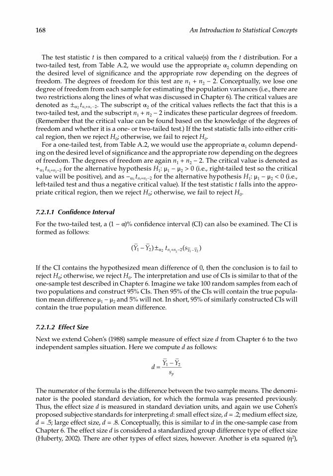
The�test�statistic�is�known�as�t′�and�is�denoted�by
�
′ = − = −+
= −
+−t
Y Ys
Y Y
s s
Y Y
sn
sn
Y Y Y Y
1 2 1 2
2 2
1 2
12
1
22
2
1 2 1 2
whereY–
1�and�Y–
2�are�the�means�for�samples�1�and�2,�respectivelysY12 �and� sY2
2 �are�the�variance�errors�of�the�means�for�samples�1�and�2,�respectively
Here�we�see�that�the�denominator�of�this�test�statistic�is�conceptually�similar�to�the�one-sample�t�and�the�independent�t�test�statistics��The�variance�errors�of�the�mean�are�com-puted�for�each�group�by
�s
snY1
2 12
1=
�s
snY2
2 22
2=
where� s12 �and� s22 �are�the�sample�variances�for�groups�1�and�2,�respectively��The�square�root�
of�the�variance�error�of�the�mean�is�the�standard�error�of�the�mean�(i�e�,� sY1�and� sY2
)��Thus,�we�see�that�rather�than�take�a�pooled�or�weighted�average�of�the�two�sample�variances�as�we�did�with�the�independent�t�test,�the�two�sample�variances�are�treated�separately�with�the�Welch�t′�test�
The�test�statistic�t′�is�then�compared�to�a�critical�value(s)�from�the�t�distribution�in�Table�A�2��We�again�use�the�appropriate�α�column�depending�on�the�desired�level�of�significance�and�whether�the�test�is�one-�or�two-tailed�(i�e�,�α1�and�α2),�and�the�appropriate�row�for�the�degrees�of�freedom��The�degrees�of�freedom�for�this�test�are�a�bit�more�complicated�than�for�the�independent�t�test��The�degrees�of�freedom�are�adjusted�from�n1�+�n2�−�2�for�the�independent�t�test�to�the�following�value�for�the�Welch�t′�test:
�
ν =+( )
( )−
+( )
−
s s
s
n
s
n
Y Y
Y Y
1 2
1 2
2 2 2
2 2
1
2 2
21 1
The�degrees�of� freedom�ν� are�approximated�by� rounding� to� the�nearest�whole�number�prior� to�using�the�table�� If� the� test�statistic� falls� into�a�critical�region,� then�we�reject�H0;�otherwise,�we�fail�to�reject�H0�
For�the�two-tailed�test,�a�(1�−�α)%�CI�can�also�be�examined��The�CI�is�formed�as�follows:
� ( ) ( )Y Y t sY Y1 2 2 1 2− ± −α ν
If�the�CI�contains�the�hypothesized�mean�difference�of�0,�then�the�conclusion�is�to�fail�to�reject�H0;�otherwise,�we�reject�H0��Thus,�interpretation�of�this�CI�is�the�same�as�with�the�independent�t�test�
174 An Introduction to Statistical Concepts
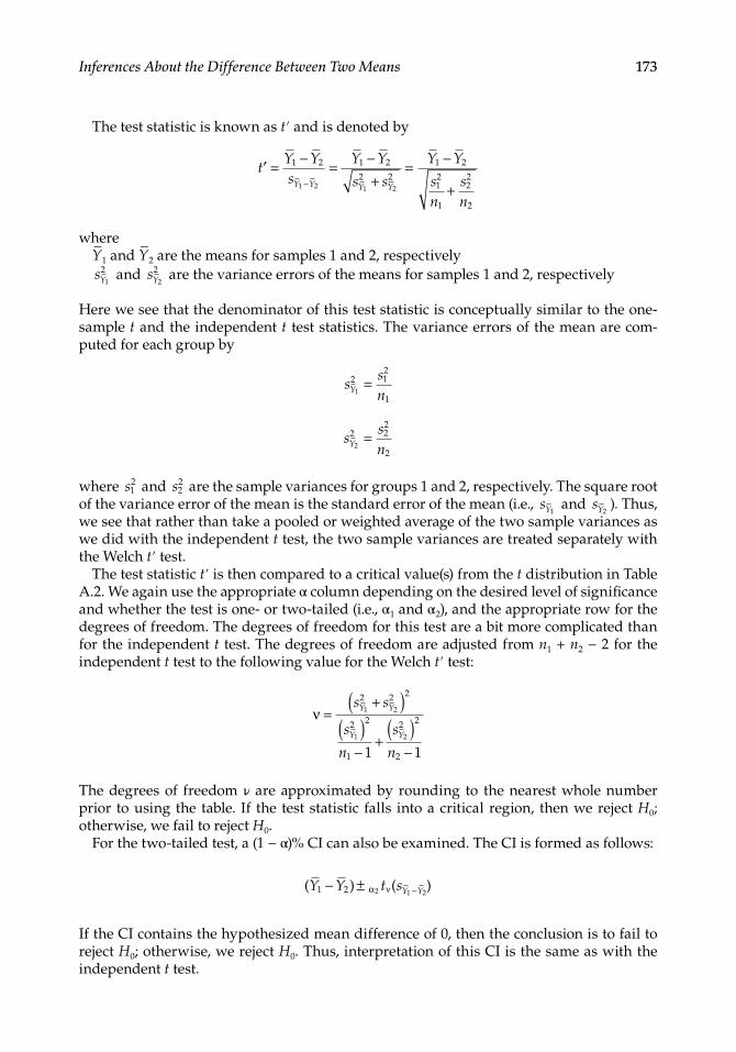
Consider�again� the�example�cholesterol�data�where� the�sample�variances�were� some-what�different�and�the�sample�sizes�were�different��The�variance�errors�of�the�mean�are�computed�for�each�sample�as�follows:
�s
snY1
2 12
1
364 28578
45 5357= = =..
�s
snY2
2 22
2
913 636312
76 1364= = =..
The�t′�test�statistic�is�computed�as
�
′ = −+
= −+
= − = −tY Y
s sY Y
1 2
2 21 2
185 21545 5357 76 1364
3011 0305
2 719. . .
. 77
Finally,�the�degrees�of�freedom�ν�are�determined�to�be
�
ν =+( )
( )−
+( )
−
= +s s
s
n
s
n
Y Y
Y Y
1 2
1 2
2 2 2
2 2
1
2 2
2
2
1 1
45 5357 76 13644( . . )
( 55 53578 1
76 136412 1
17 98382 2. ) ( . ).
−+
−
=
which�is�rounded�to�18,�the�nearest�whole�number��The�degrees�of�freedom�remain�18�as�they�were�for�the�independent�t�test,�and�thus,�the�critical�values�are�still�+2�101�and�−2�101��As�the�test�statistic�falls�beyond�the�critical�values�as�shown�in�Figure�7�1,�we�therefore�reject�the�null�hypothesis�that�the�means�are�equal�in�favor�of�the�alternative�that�the�means�are�not�equal��Thus,�as�with�the�independent�t�test,�with�the�Welch�t′�test,�we�conclude�that�the�mean�cholesterol�levels�for�males�and�females�are�not�equal�at�the��05�level�of�significance��In�this�particular�example,�then,�we�see�that�the�unequal�sample�variances�and�unequal�sample�sizes�did�not�alter�the�outcome�when�comparing�the�independent�t�test�result�with�the�Welch�t′�test�result��However,�note�that�the�results�for�these�two�tests�may�differ�with�other�data�
Finally,�the�95%�CI�can�be�examined��For�the�example,�the�CI�is�formed�as�follows:
� ( ) ( ) ( ) . ( . ) .Y Y t sY Y1 2 2 1 2185 215 2 101 11 0305 30 23 1751− ± = − ± = − ± =−α ν (( . , . )− −53 1751 6 8249
As�the�CI�does�not�contain�the�hypothesized�mean�difference�value�of�0,�then�we�would�again� reject� the�null�hypothesis�and�conclude� that� the�mean�gender�difference�was�not�equal�to�0�at�the��05�level�of�significance�(p�<��05)�
7.2.3 Recommendations
The�following�four�recommendations�are�made�regarding�the�two�independent�samples�case��Although� there� is�no� total� consensus� in� the�field,�our� recommendations� take� into�account,�as�much�as�possible,�the�available�research�and�statistical�software��First,� if�the�normality� assumption� is� satisfied,� the� following� recommendations� are� made:� (a)� the�

175Inferences About the Difference Between Two Means
independent�t�test�is�recommended�when�the�homogeneity�of�variance�assumption�is�met;�(b)�the�independent�t�test�is�recommended�when�the�homogeneity�of�variance�assumption�is�not�met�and�when�there�are�an�equal�number�of�observations�in�the�samples;�and�(c)�the�Welch�t′�test�is�recommended�when�the�homogeneity�of�variance�assumption�is�not�met�and�when�there�are�an�unequal�number�of�observations�in�the�samples�
Second,�if�the�normality�assumption�is�not�satisfied,�the�following�recommendations�are�made:�(a)�if�the�homogeneity�of�variance�assumption�is�met,�then�the�independent�t�test�using�ranked�scores�(Conover�&�Iman,�1981),�rather�than�raw�scores,�is�recommended;�and�(b)�if�homogeneity�of�variance�assumption�is�not�met,�then�the�Welch�t′�test�using�ranked�scores�is�recommended,�regardless�of�whether�there�are�an�equal�number�of�observations�in�the�samples��Using�ranked�scores�means�you�rank�order�the�observations�from�highest�to�lowest�regardless�of�group�membership,�then�conduct�the�appropriate�t�test�with�ranked�scores�rather�than�raw�scores�
Third,�the�dependent�t�test�is�recommended�when�there�is�some�dependence�between�the�groups�(e�g�,�matched�pairs�or�the�same�individuals�measured�on�two�occasions),�as�described� later� in� this�chapter��Fourth,� the�nonparametric�Mann-Whitney-Wilcoxon�test�is�not�recommended��Among�the�disadvantages�of�this�test�are�that�(a)�the�critical�values�are�not�extensively�tabled,�(b)�tied�ranks�can�affect�the�results�and�no�optimal�procedure�has�yet�been�developed�(Wilcox,�1996),�and�(c)�Type�I�error�appears�to�be�inflated�regard-less�of�the�status�of�the�assumptions�(Zimmerman,�2003)��For�these�reasons,�the�Mann–Whitney–Wilcoxon� test� is� not� further� described� here�� Note� that� most� major� statistical�packages,�including�SPSS,�have�options�for�conducting�the�independent�t�test,�the�Welch�t′�test,�and�the�Mann-Whitney-Wilcoxon�test��Alternatively,�one�could�conduct�the�Kruskal–Wallis�nonparametric�one-factor�ANOVA,�which�is�also�based�on�ranked�data,�and�which�is�appropriate�for�comparing�the�means�of�two�or�more�independent�groups��This�test�is�considered�more�fully�in�Chapter�11��These�recommendations�are�summarized�in�Box�7�1�
STOp aNd ThINk bOx 7.1
Recommendations�for�the�Independent�and�Dependent�Samples�Tests�Based�on�Meeting�or Violating�the�Assumption�of�Normality
Assumption IndependentSamplesTests DependentSamplesTests
Normality�is�met •��Use�the�independent�t�test�when�homogeneity�of�variances�is�met
•�Use�the�dependent�t�test
•��Use�the�independent�t�test�when�homogeneity�of�variances�is�not�met,�but�there�are�equal�sample�sizes�in�the�groups
•��Use�the�Welch�t′�test�when�homogeneity�of�variances�is�not�met�and�there�are�unequal�sample�sizes�in�the�groups
Normality�is�not�met •��Use�the�independent�t�test�with�ranked�scores�when�homogeneity�of�variances�is�met
•��Use�the�Welch�t′�test�with�ranked�scores�when�homogeneity�of�variances�is�not�met,�regardless�of�equal�or�unequal�sample�sizes�in�the�groups
•��Use�the�Kruskal–Wallis�nonparametric�procedure
•��Use�the�dependent�t�test�with�ranked�scores,�or�alternative�procedures�including�bootstrap�methods,�trimmed�means,�medians,�or�Stein’s�method
•��Use�the�Wilcoxon�signed�ranks�test�when�data�are�both�nonnormal�and�have�extreme�outliers
•��Use�the�Friedman�nonparametric�procedure

176 An Introduction to Statistical Concepts
7.3 InferencesAboutTwoDependentMeans
In�this�section,�two�inferential�tests�of�the�difference�between�two�dependent�means�are�described,� the�dependent� t� test�and�briefly� the�Wilcoxon�signed� ranks� test��The� section�concludes�with�a�list�of�recommendations�
7.3.1 dependent t Test
As�you�may�recall,�the�dependent�t�test�is�appropriate�to�use�when�there�are�two�samples�that�are�dependent—the�individuals�in�sample�1�have�some�relationship�to�the�individuals�in�sample�2��First,�we�need�to�determine�the�conditions�under�which�the�dependent�t�test�is�appropriate��In�part,�this�has�to�do�with�the�statistical�assumptions�associated�with�the�test�itself—that�is,�(a)�normality�of�the�distribution�of�the�differences�of�the�dependent�variable�Y,�(b)�homogeneity�of�variance�of�the�two�populations,�and�(c)�independence�of�the�obser-vations�within�each�sample��Like�the�independent�t�test,�the�dependent�t�test�is�reasonably�robust�to�violation�of�the�normality�assumption,�as�we�show�later��Because�this�is�a�test�of�means,�the�dependent�variable�must�be�measured�on�an�interval�or�ratio�scale��For�example,�the�same�individuals�may�be�measured�at�two�points�in�time�on�the�same�interval-scaled�pretest�and�posttest,�or�some�matched�pairs�(e�g�,�twins�or�husbands–wives)�may�be�assessed�with�the�same�ratio-scaled�measure�(e�g�,�weight�measured�in�pounds)�
Although�there�are�several�methods�for�computing�the�test�statistic�t,�the�most�direct�method�and�the�one�most�closely�aligned�conceptually�with�the�one-sample�t�test�is�as�follows:
�t
dsd
=
whered–�is�the�mean�difference
sd–�is�the�standard�error�of�the�mean�difference
Conceptually,� this� test�statistic� looks� just� like�the�one-sample�t� test�statistic,�except�now�that�the�notation�has�been�changed�to�denote�that�we�are�dealing�with�difference�scores�rather�than�raw�scores�
The�standard�error�of�the�mean�difference�is�computed�by
�s
sndd=
wheresd�is�the�standard�deviation�of�the�difference�scores�(i�e�,�like�any�other�standard�devia-
tion,�only�this�one�is�computed�from�the�difference�scores�rather�than�raw�scores)n�is�the�total�number�of�pairs
Conceptually,�this�standard�error�looks�just�like�the�standard�error�for�the�one-sample�t�test��If�we�were�doing�hand�computations,�we�would�compute�a�difference�score�for�each�pair�of�scores�(i�e�,�Y1�−�Y2)��For�example,�if�sample�1�were�wives�and�sample�2�were�their�husbands,�then�we�calculate�a�difference�score�for�each�couple��From�this�set�of�difference�scores,�we�then�compute�the�mean�of�the�difference�scores�d–�and�standard�deviation�of�the�difference�

177Inferences About the Difference Between Two Means
scores�sd��This�leads�us�directly�into�the�computation�of�the�t�test�statistic��Note�that�although�there�are�n�scores�in�sample�1,�n�scores�in�sample�2,�and�thus�2n�total�scores,�there�are�only�n�difference�scores,�which�is�what�the�analysis�is�actually�based�upon�
The�test�statistic�t�is�then�compared�with�a�critical�value(s)�from�the�t�distribution��For�a�two-tailed�test,�from�Table�A�2,�we�would�use�the�appropriate�α2�column�depending�on�the�desired�level�of�significance�and�the�appropriate�row�depending�on�the�degrees�of�free-dom��The�degrees�of�freedom�for�this�test�are�n�−�1��Conceptually,�we�lose�one�degree�of�freedom�from�the�number�of�differences�(or�pairs)�because�we�are�estimating�the�popula-tion�variance�(or�standard�deviation)�of�the�difference��Thus,�there�is�one�restriction�along�the� lines� of� our� discussion� of� degrees� of� freedom� in� Chapter� 6�� The� critical� values� are�denoted�as�± −α2 1tn ��The�subscript,�α2,�of�the�critical�values�reflects�the�fact�that�this�is�a�two-tailed�test,�and�the�subscript�n�−�1�indicates�the�degrees�of�freedom��If�the�test�statistic�falls�into�either�critical�region,�then�we�reject�H0;�otherwise,�we�fail�to�reject�H0�
For�a�one-tailed�test,�from�Table�A�2,�we�would�use�the�appropriate�α1�column�depending�on�the�desired�level�of�significance�and�the�appropriate�row�depending�on�the�degrees�of�freedom��The�degrees�of�freedom�are�again�n�−�1��The�critical�value�is�denoted�as�+ −α1 1tn �for�the�alternative�hypothesis�H1:�μ1�−�μ2�>�0�and�as� − −α1 1tn �for�the�alternative�hypothesis�H1:�μ1�−�μ2�<�0��If�the�test�statistic�t�falls�into�the�appropriate�critical�region,�then�we�reject�H0;�otherwise,�we�fail�to�reject�H0�
7.3.1.1 Confidence Interval
For�the�two-tailed�test,�a�(1�−�α)%�CI�can�also�be�examined��The�CI�is�formed�as�follows:
� d t sn d± −α 2 1( )
If�the�CI�contains�the�hypothesized�mean�difference�of�0,�then�the�conclusion�is�to�fail�to�reject�H0;�otherwise,�we�reject�H0��The�interpretation�of�these�CIs�is�the�same�as�those�previ-ously�discussed�for�the�one-sample�t�and�the�independent�t�
7.3.1.2 Effect Size
The�effect�size�can�be�measured�using�Cohen’s�(1988)�d�computed�as�follows:
�Cohen d
dsd
=
where�Cohen’s�d�is�simply�used�to�distinguish�among�the�various�uses�and�slight�differ-ences�in�the�computation�of�d��Interpretation�of�the�value�of�d�would�be�the�same�as�for�the�one-sample�t�and�the�independent�t�previously�discussed—specifically,�the�number�of�standard�deviation�units�for�which�the�mean(s)�differ(s)�
7.3.1.3 Example of the Dependent t Test
Let�us�consider�an�example�for�purposes�of�illustrating�the�dependent�t�test��Ten�young�swimmers�participated�in�an�intensive�2�month�training�program��Prior�to�the�program,�each�swimmer�was�timed�during�a�50�meter�freestyle�event��Following�the�program,�the�

178 An Introduction to Statistical Concepts
same�swimmers�were�timed�in�the�50�meter�freestyle�event�again��This�is�a�classic�pretest-posttest�design��For�illustrative�purposes,�we�will�conduct�a�two-tailed�test��However,�a�case�might�also�be�made�for�a�one-tailed�test�as�well,� in� that� the�coach�might�want� to�see�improvement�only��However,�conducting�a�two-tailed�test�allows�us�to�examine�the�CI�for�purposes�of�illustration��The�raw�scores,�the�difference�scores,�and�the�mean�and�standard�deviation�of�the�difference�scores�are�shown�in�Table�7�2��The�pretest�mean�time�was�64�seconds�and�the�posttest�mean�time�was�59�seconds�
To�determine�our�test�statistic�value,�t,�first�we�compute�the�standard�error�of�the�mean�difference�as�follows:
�s
sndd= = =2 1602
100 6831
..
Next,�using�this�value�for�the�denominator,�the�test�statistic�t�is�then�computed�as�follows:
�t
dsd
= = =50 6831
7 3196.
.
We�then�use�Table�A�2�to�determine�the�critical�values��As�there�are�nine�degrees�of�free-dom�(n�−�1�=�10�−�1�=�9),�using�α�=��05�and�a�two-tailed�or�nondirectional�test,�we�find�the�critical�values�using�the�appropriate�α2�column�to�be�+2�262�and�−2�262��Since�the�test�sta-tistic�falls�beyond�the�critical�values,�as�shown�in�Figure�7�2,�we�reject�the�null�hypothesis�that�the�means�are�equal�in�favor�of�the�nondirectional�alternative�that�the�means�are�not�equal��Thus,�we�conclude�that�the�mean�swimming�performance�changed�from�pretest�to�posttest�at�the��05�level�of�significance�(p�<��05)�
The�95%�CI�is�computed�to�be�the�following:
� d t sn d± = ± = ± =−α 2 1 5 2 262 0 6831 5 1 5452 3 4548 6 5452( ) . ( . ) . ( . , . )
Table 7.2
Swimming�Data�for�Dependent�Samples
SwimmerPretestTime(inSeconds)
PosttestTime(inSeconds) Difference(d)
1 58 54 (i�e�,�58�−�54)�=�42 62 57 53 60 54 64 61 56 55 63 61 26 65 59 67 66 64 28 69 62 79 64 60 4
10 72 63 9d–�=�5�0000
sd�=�2�1602

179Inferences About the Difference Between Two Means
As�the�CI�does�not�contain�the�hypothesized�mean�difference�value�of�0,�we�would�again�reject�the�null�hypothesis�and�conclude�that�the�mean�pretest-posttest�difference�was�not�equal�to�0�at�the��05�level�of�significance�(p�<��05)�
The�effect�size�is�computed�to�be�the�following:
�Cohen d
dsd
= = =52 1602
2 3146.
.
which� is� interpreted� as� there� is� approximately� a� two�and�one-third� standard�deviation�difference�between�the�pretest�and�posttest�mean�swimming�times,�a�very�large�effect�size�according�to�Cohen’s�subjective�standard�
7.3.1.4 Assumptions
Let�us�return�to�the�assumptions�of�normality,�independence,�and�homogeneity�of�vari-ance��For� the�dependent� t� test,� the�assumption�of�normality� is�met�when�the�difference�scores�are�normally�distributed��Normality�of� the�difference�scores�can�be�examined�as�discussed�previously—graphical�methods� (such�as�stem-and-leaf�plots,�box�plots,�histo-grams,�and/or�Q–Q�plots),�statistical�procedures�such�as�the�S–W�test�(1965),�and/or�skew-ness�and�kurtosis�statistics��The�assumption�of�independence�is�met�when�the�cases�in�our�sample�have�been�randomly�selected�from�the�population��If�the�independence�assump-tion�is�not�met,�then�probability�statements�about�the�Type�I�and�Type�II�errors�will�not�be�accurate;�in�other�words,�the�probability�of�a�Type�I�or�Type�II�error�may�be�increased�as�a�result�of�the�assumption�not�being�met��Homogeneity�of�variance�refers�to�equal�variances�of�the�two�populations��In�later�chapters,�we�will�examine�procedures�for�formally�testing�for�equal�variances��For�the�moment,�if�the�ratio�of�the�smallest�to�largest�sample�variance�is�within�1:4,�then�we�have�evidence�to�suggest�the�assumption�of�homogeneity�of�vari-ances�is�met��Research�has�shown�that�the�effect�of�heterogeneity�(i�e�,�unequal�variances)�is�minimal�when�the�sizes�of�the�two�samples,�n1�and�n2,�are�equal,�as�is�the�case�with�the�dependent�t�test�by�definition�(unless�there�are�missing�data)�
α = .025
–2.262Criticalvalue
+2.262Criticalvalue
+7.3196t test
statisticvalue
α = .025
FIGuRe 7.2Critical� regions� and� test� statistic� for� the�swimming�example�

180 An Introduction to Statistical Concepts
7.3.2 Recommendations
The� following� three� recommendations�are�made�regarding� the� two�dependent� samples�case��First,�the�dependent�t�test�is�recommended�when�the�normality�assumption�is�met��Second,�the�dependent�t�test�using�ranks�(Conover�&�Iman,�1981)�is�recommended�when�the�normality�assumption�is�not�met��Here�you�rank�order�the�difference�scores�from�high-est�to�lowest,�then�conduct�the�test�on�the�ranked�difference�scores�rather�than�on�the�raw�difference�scores��However,�more�recent�research�by�Wilcox�(2003)�indicates�that�power�for�the�dependent�t�can�be�reduced�even�for�slight�departures�from�normality��Wilcox�recom-mends�several�procedures�not�readily�available�and�beyond�the�scope�of�this�text�(boot-strap�methods,�trimmed�means,�medians,�Stein’s�method)��Keep�in�mind,�though,�that�the�dependent�t�test�is�fairly�robust�to�nonnormality�in�most�situations�
Third,�the�nonparametric�Wilcoxon�signed�ranks�test�is�recommended�when�the�data�are�nonnormal�with�extreme�outliers�(one�or�a�few�observations�that�behave�quite�differ-ently�from�the�rest)��However,�among�the�disadvantages�of�this�test�are�that�(a)�the�criti-cal�values�are�not�extensively�tabled�and�two�different�tables�exist�depending�on�sample�size,� and� (b)� tied� ranks� can�affect� the� results� and�no�optimal�procedure�has�yet�been�developed� (Wilcox,� 1996)�� For� these� reasons,� the� details� of� the� Wilcoxon� signed� ranks�test�are�not�described�here��Note� that�most�major�statistical�packages,� including�SPSS,�include�options�for�conducting�the�dependent�t�test�and�the�Wilcoxon�signed�ranks�test��Alternatively,�one�could�conduct�the�Friedman�nonparametric�one-factor�ANOVA,�also�based�on�ranked�data,�and�which�is�appropriate�for�comparing�two�or�more�dependent�sample�means��This�test�is�considered�more�fully�in�Chapter�15��These�recommendations�are�summarized�in�Box�7�1�
7.4 SPSS
Instructions�for�determining�the�independent�samples�t�test�using�SPSS�are�presented�first��This� is� followed�by�additional�steps�for�examining�the�assumption�of�normality�for�the�independent�t�test��Next,�instructions�for�determining�the�dependent�samples�t�test�using�SPSS�are�presented�and�are�then�followed�by�additional�steps�for�examining�the�assump-tions�of�normality�and�homogeneity�
Independent t Test
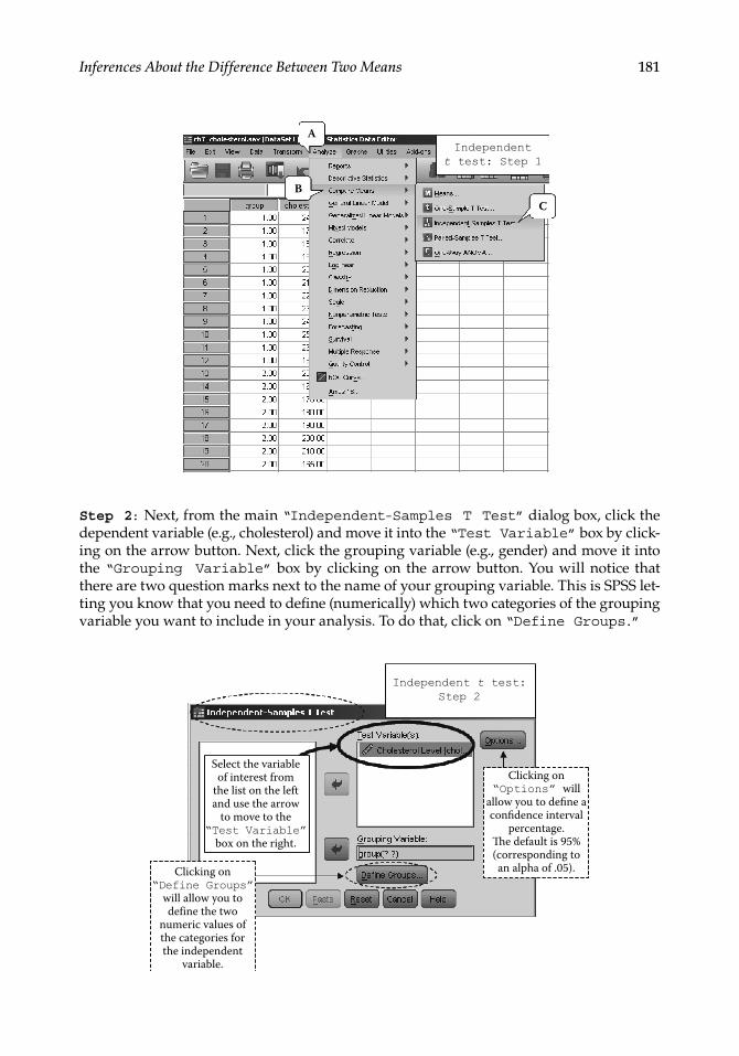
Step 1:� In� order� to� conduct� an� independent� t� test,� your� dataset� needs� to� include� a�dependent�variable�Y�that�is�measured�on�an�interval�or�ratio�scale�(e�g�,�cholesterol),�as�well�as�a�grouping�variable�X�that�is�measured�on�a�nominal�or�ordinal�scale�(e�g�,�gen-der)��For�the�grouping�variable,�if�there�are�more�than�two�categories�available,�only�two�categories�can�be�selected�when�running�the�independent�t�test�(the�ANOVA�is�required�for�examining�more�than�two�categories)��To�conduct�the�independent�t� test,�go�to�the�“Analyze”�in�the�top�pulldown�menu,�then�select�“Compare Means,”�and�then�select�“Independent-Samples T Test.”�Following�the�screenshot�(step�1)�as�follows�pro-duces�the�“Independent-Samples T Test”�dialog�box�
181Inferences About the Difference Between Two Means
A
BC
Independentt test: Step 1
Step 2:�Next,�from�the�main�“Independent-Samples T Test”�dialog�box,�click�the�dependent�variable�(e�g�,�cholesterol)�and�move�it�into�the�“Test Variable”�box�by�click-ing�on�the�arrow�button��Next,�click�the�grouping�variable�(e�g�,�gender)�and�move�it�into�the�“Grouping Variable”�box�by�clicking�on� the�arrow�button��You�will�notice� that�there�are�two�question�marks�next�to�the�name�of�your�grouping�variable��This�is�SPSS�let-ting�you�know�that�you�need�to�define�(numerically)�which�two�categories�of�the�grouping�variable�you�want�to�include�in�your�analysis��To�do�that,�click�on�“Define Groups.”
Clicking on“Options” will
allow you to define aconfidence interval
percentage.e default is 95%(corresponding toan alpha of .05).
Select the variableof interest from
the list on the leftand use the arrow
to move to the“Test Variable”
box on the right.
Clicking on“Define Groups”
will allow you todefine the two
numeric values ofthe categories forthe independent
variable.
Independent t test:Step 2

182 An Introduction to Statistical Concepts
Step 3:�From�the�“Define Groups”�dialog�box,�enter�the�numeric�value�designated�for�each�of�the�two�categories�or�groups�of�your�independent�variable��Where�it�says�“Group 1,”�type�in�the�value�designated�for�your�first�group�(e�g�,�1,�which�in�our�case�indicated�that�the�individual�was�a�female),�and�where�it�says�“Group 2,”�type�in�the�value�desig-nated�for�your�second�group�(e�g�,�2,�in�our�example,�a�male)�(see�step�3�screenshot)�
Independent t test:Step 3
Click�on�“Continue”�to�return�to�the�original�dialog�box�(see�step�2�screenshot)�and�then�click�on�“OK”�to�run�the�analysis��The�output�is�shown�in�Table�7�3�
Changing the alpha level (optional):�The�default�alpha�level�in�SPSS�is��05,�and�thus,�the�default�corresponding�CI�is�95%��If�you�wish�to�test�your�hypothesis�at�an�alpha�level�other�than��05�(and�thus�obtain�CIs�other�than�95%),�click�on�the�“Options”�button�located�in�the�top�right�corner�of�the�main�dialog�box�(see�step�2�screenshot)��From�here,�the�CI�percentage�can�be�adjusted�to�correspond�to�the�alpha�level�at�which�you�wish�your�hypothesis�to�be�tested�(see�Chapter�6�screenshot�step�3)��(For�purposes�of�this�example,�the�test�has�been�generated�using�an�alpha�level�of��05�)
Interpreting the output:�The�top�table�provides�various�descriptive�statistics�for�each�group,�while� the�bottom�box�gives� the�results�of� the�requested�procedure��There�you�see�the�following�three�different� inferential� tests� that�are�automatically�provided:�(1)�Levene’s� test�of� the�homogeneity�of�variance�assumption� (the�first� two�columns�of�results),�(2)�the�independent�t�test�(which�SPSS�calls�“Equal variances assumed”)�(the�top�row�of�the�remaining�columns�of�results),�and�(3)�the�Welch�t′�test�(which�SPSS�calls�“Equal variances not assumed”)�(the�bottom�row�of�the�remaining�columns�of�results)�
The�first� interpretation�that�must�be�made�is� for�Levene’s�test�of�equal�variances��The�assumption� of� equal� variances� is� met� when� Levene’s� test� is� not� statistically� significant��We�can�determine�statistical�significance�by�reviewing�the�p�value�for�the�F� test��In�this�example,�the�p�value�is��090,�greater�than�our�alpha�level�of��05�and�thus�not�statistically�significant��Levene’s�test�tells�us�that�the�variance�for�cholesterol�level�for�males�is�not�sta-tistically�significantly�different�than�the�variance�for�cholesterol�level�for�females��Having�met�the�assumption�of�equal�variances,�the�values�in�the�rest�of�the�table�will�be�drawn�from�the�row�labeled�“Equal Variances Assumed.”�Had�we�not�met�the�assumption�of�equal�variances�(p�<�α),�we�would�report�Welch�t′�for�which�the�statistics�are�presented�on�the�row�labeled�“Equal Variances Not Assumed.”
After� determining� that� the� variances� are� equal,� the� next� step� is� to� examine� the�results�of�the�independent�t�test��The�t�test�statistic�value�is�−2�4842,�and�the�associated�p�value�is��023��Since�p�is�less�than�α,�we�reject�the�null�hypothesis��There�is�evidence�to�suggest�that�the�mean�cholesterol�level�for�males�is�different�than�the�mean�cholesterol�level�for�females�

183Inferences About the Difference Between Two Means
Table 7.3
SPSS�Results�for�Independent�t�Test
Group Statistics
Gender N Mean Std. Deviation Std. Error Mean
Female 8 185.0000 19.08627 6.74802Cholesterol level
Male 12 215.0000 30.22642 8.72562
Independent Samples Test
Levene's Test forEquality of Variances t-Test for Equality of Means
95% Confidence Interval of the Difference
F Sig. t dfSig.
(2-Tailed)Mean
Difference Std. Error Difference Lower Upper
3.201 .090 –2.484 .023 –30.00000 12.07615 –55.37104
–2.720
18
17.984 .014 –30.00000 11.03051 –53.17573
–4.62896
– 6.82427
“t” is the t test statistic value.�e t value in the top row is used when theassumption of equal variances has been met andis calculated as:
The t value in the bottom row is the Welch t΄andis used when the assumption of equal varianceshas not been met.
�e table labeled “Group Statistics”provides basic descriptive statistics for the
dependent variable by group.
SPSS reports the95% confidence interval ofthe difference. This is
interpreted to mean that 95% of the CIs generated
across samples will containthe true population mean
difference of 0.
�e F test (and p value) of Levene’s Test forEquality of Variances is reviewed to determine
if the equal variances assumption has beenmet. �e result of this test determines which
row of statistics to utilize. In this case, wemeet the assumption and use the statistics
reported in the top row.
“Sig.” is the observed p valuefor the independent t test.
It is interpreted as: there is less than a 3% probability of a samplemean difference of –30 or greater
occurring by chance if the nullhypothesis is really true (i.e., if
the population mean difference is 0).
�e mean difference is simply the differencebetween the sample mean cholesterol values. In other words, 185 – 215 = – 30
The standard error of the mean difference is calculated as:
=–sY1sp n1 n2
11+
df are thedegrees of freedom.For theindependentsamples t test,they arecalculated as
Equalvariancesassumed
Cholesterollevel
Equalvariances
not assumed
Y2
n1 + n2 – 2.
–2.48412.075
Y1 – Y2t sY1 – Y2
185 – 215===
184 An Introduction to Statistical Concepts
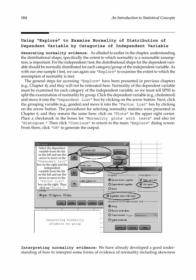
Using “Explore” to Examine Normality of Distribution of Dependent Variable by Categories of Independent Variable
Generating normality evidence: As�alluded�to�earlier�in�the�chapter,�understanding�the�distributional�shape,�specifically�the�extent�to�which�normality�is�a�reasonable�assump-tion,�is�important��For�the�independent�t�test,�the�distributional�shape�for�the�dependent�vari-able�should�be�normally�distributed�for�each�category/group�of�the�independent�variable��As�with�our�one-sample�t�test,�we�can�again�use�“Explore”�to�examine�the�extent�to�which�the�assumption�of�normality�is�met�
The�general�steps�for�accessing�“Explore”�have�been�presented�in�previous�chapters�(e�g�,�Chapter�4),�and�they�will�not�be�reiterated�here��Normality�of�the�dependent�variable�must�be�examined�for�each�category�of�the�independent�variable,�so�we�must�tell�SPSS�to�split�the�examination�of�normality�by�group��Click�the�dependent�variable�(e�g�,�cholesterol)�and�move�it�into�the�“Dependent List”�box�by�clicking�on�the�arrow�button��Next,�click�the�grouping�variable�(e�g�,�gender)�and�move�it�into�the�“Factor List”�box�by�clicking�on�the�arrow�button��The�procedures�for�selecting�normality�statistics�were�presented�in�Chapter�6,�and�they�remain�the�same�here:�click�on�“Plots”� in� the�upper�right�corner��Place� a� checkmark� in� the� boxes� for�“Normality plots with tests”� and� also� for�“Histogram.”�Then�click�“Continue”�to�return�to�the�main�“Explore”�dialog�screen��From�there,�click�“OK”�to�generate�the�output�
Select the dependentvariable from the list
on the left and use the arrow to move to the“Dependent List”box on the right and the
independentvariable from the list
on the left and use thearrow to move to the“Factor List”
box on the right. �enclick on “Plots.”
Generating normality
evidence by group
Interpreting normality evidence:�We�have�already�developed�a�good�under-standing�of�how�to�interpret�some�forms�of�evidence�of�normality�including�skewness�

185Inferences About the Difference Between Two Means
and�kurtosis,�histograms,�and�boxplots��As�we�examine� the�“Descriptives”� table,�we�see� the� output� for� the� cholesterol� statistics� is� separated� for� male� (top� portion)� and�female�(bottom�portion)�
Mean95% Con�dence intervalfor mean
5% Trimmed meanMedianVarianceStd. deviationMinimumMaximumRangeInterquartile rangeSkewnessKurtosisMean95% Con�dence intervalfor mean
5% Trimmed meanMedianVarianceStd. deviationMinimum
MaximumRangeInterquartile rangeSkewnessKurtosis
FemaleLower boundUpper bound
Lower boundUpper bound
Cholesterol level Male
GenderDescriptives
Statistic Std. Error215.0000195.7951234.2049
215.0000215.0000
913.636
170.00260.00
90.0057.50
.000–1.446
185.0000169.0435200.9565185.0000185.0000
364.28619.08627
160.00210.00
50.0037.50
.000–1.790
1.2326.74802
.637
30.22642
8.72562
.7521.481
The� skewness� statistic� of� cholesterol� level� for� the� males� is� �000� and� kurtosis� is�−1�446—both�within�the�range�of�an�absolute�value�of�2�0,�suggesting�some�evidence�of�normality�of� the�dependent�variable� for�males��Evidence�of�normality� for� the�dis-tributional�shape�of�cholesterol�level�for�females�is�also�present:�skewness�=��000�and�kurtosis�=�−1�790�
The�histogram�of�cholesterol�level�for�males�is�not�exactly�what�most�researchers�would�consider� a� classic� normally� shaped� distribution�� Although� the� histogram� of� cholesterol�level�for�females�is�not�presented�here,�it�follows�a�similar�distributional�shape�

186 An Introduction to Statistical Concepts
2.0
1.5
1.0
Freq
uenc
y
0.5
0.0160.00 180.00 200.00 220.00
Cholesterol level240.00 260.00
Histogram for group = Male
Mean = 215.00Std. dev. = 30.226N = 12
There�are�a�few�other�statistics�that�can�be�used�to�gauge�normality�as�well��Our�formal�test�of�normality,�the�Shapiro–Wilk�test�(SW)�(Shapiro�&�Wilk,�1965),�provides�evidence�of�the�extent�to�which�our�sample�distribution�is�statistically�different�from�a�normal�distri-bution��The�output�for�the�S–W�test�is�presented�in�the�following�and�suggests�that�our�sample�distribution�for�cholesterol�level�is�not�statistically�significantly�different�than�what�would�be�expected�from�a�normal�distribution—and�this�is�true�for�both�males�(SW�=��949,�df�=�12,�p�=��617)�and�females�(SW�=��931,�df�=�8,�p�=��525)�
Gender
MaleFemale
Cholesterol levelStatistic Statisticdf
Tests of Normality
Kolmogorov–Smirnova
dfShapiro–Wilk
Sig. Sig..129.159 8
12
8
12 .617.525
.200
.200 .931.949
a Lilliefors significance correction* This is a lower bound of the true significance.
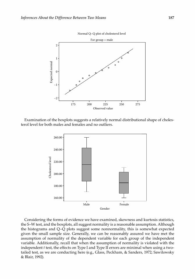
Quantile–quantile�(Q–Q)�plots�are�also�often�examined�to�determine�evidence�of�nor-mality�� Q–Q� plots� are� graphs� that� plot� quantiles� of� the� theoretical� normal� distribution�against�quantiles�of�the�sample�distribution��Points�that�fall�on�or�close�to�the�diagonal�line�suggest�evidence�of�normality��Similar�to�what�we�saw�with�the�histogram,�the�Q–Q�plot�of�cholesterol�level�for�both�males�and�females�(although�not�shown�here)�suggests�some�nonnormality��Keep�in�mind�that�we�have�a�relatively�small�sample�size��Thus,�interpreting�the�visual�graphs�(e�g�,�histograms�and�Q–Q�plots)�can�be�challenging,�although�we�have�plenty�of�other�evidence�for�normality�
187Inferences About the Difference Between Two Means
2
1
0
–1
–2
Expe
cted
nor
mal
175 200 225Observed value
250 275
Normal Q–Q plot of cholesterol level
For group = male
Examination�of�the�boxplots�suggests�a�relatively�normal�distributional�shape�of�choles-terol�level�for�both�males�and�females�and�no�outliers�
260.00
240.00
220.00
200.00
Chol
este
rol l
evel
180.00
160.00
Male FemaleGender
Considering�the�forms�of�evidence�we�have�examined,�skewness�and�kurtosis�statistics,�the�S–W�test,�and�the�boxplots,�all�suggest�normality�is�a�reasonable�assumption��Although�the� histograms� and� Q–Q� plots� suggest� some� nonnormality,� this� is� somewhat� expected�given� the�small� sample�size��Generally,�we�can�be� reasonably�assured�we�have�met� the�assumption� of� normality� of� the� dependent� variable� for� each� group� of� the� independent�variable��Additionally,�recall�that�when�the�assumption�of�normality�is�violated�with�the�independent�t�test,�the�effects�on�Type�I�and�Type�II�errors�are�minimal�when�using�a�two-tailed�test,�as�we�are�conducting�here�(e�g�,�Glass,�Peckham,�&�Sanders,�1972;�Sawilowsky�&�Blair,�1992)�

188 An Introduction to Statistical Concepts
Dependent t Test
Step 1:�To�conduct�a�dependent�t�test,�your�dataset�needs�to�include�the�two�variables�(i�e�,�for�the�paired�samples)�whose�means�you�wish�to�compare�(e�g�,�pretest�and�posttest)��To�conduct� the�dependent� t� test,�go� to� the�“Analyze”� in� the� top�pulldown�menu,� then�select�“Compare Means,”�and�then�select�“Paired-Samples T Test.”�Following�the�screenshot�(step�1)�as�follows�produces�the�“Paired-Samples T Test”�dialog�box�
A
B
C
Dependent t test:Step 1
Step 2:�Click�both�variables�(e�g�,�pretest�and�posttest�as�variable�1�and�variable�2,�respec-tively)�and�move�them�into�the�“Paired Variables”�box�by�clicking�the�arrow�button��Both�variables�should�now�appear�in�the�box�as�shown�in�screenshot�step�2��Then�click�on�“Ok” to�run�the�analysis�and�generate�the�output�
Select the pairedsamples from the liston the left and use thearrow to move to the“PairedVariables”box on the right.Then click on “Ok.”
Dependent t test:Step 2
The�output�appears�in�Table�7�4,�where�again�the�top�box�provides�descriptive�statistics,�the�middle�box�provides�a�bivariate�correlation�coefficient,�and�the�bottom�box�gives�the�results�of�the�dependent�t�test�procedure�

189Inferences About the Difference Between Two Means
Table 7.4
SPSS�Results�for�Dependent�t�Test
Paired Samples Statistics
Mean N Std. Deviation Std. Error Mean
Pretest 64.0000 10 4.21637 1.33333Pair 1 Posttest 59.0000 10 3.62093 1.14504
Paired Samples Correlations
N Correlation Sig.
Pair 1 Pretest and posttest 10 .859 .001
Paired Samples Test
Paired Differences
95% Confidence Interval of the
Difference
MeanStd.
Deviation Std. Error
Mean Lower Upper t df Sig. (2-Tailed)Pair 1 Pretest -
posttest5.00000 2.16025 .68313 3.45465 6.54535 7.319 9 .000
�e table labeled “Paired SamplesStatistics” provides basic descriptive
statistics for the paired samples.
The table labeled “Paired SamplesCorrelations” provides the Pearson
Product Moment CorrelationCoefficient value, a bivariate
correlation coefficient, between thepretest and posttest values.
In this example, there is a strongcorrelation (r = .859) and it is
statistically significant ( p = .001).�e values in this section ofthe table are calculated basedon paired differences (i.e., the
difference values betweenpretest and posttest scores).
“Sig.” is the observed p value forthe dependent t test.
It is interpreted as:there is less than a 1%probability of a samplemean difference of 5 or
greater occurring bychance if the null
hypothesis is really true(i.e., if the populationmean difference is 0).
df are thedegrees offreedom.For the
dependentsamples
t test, they arecalculated as
n – 1.
“t” is the t test statistic value.The t value is calculated as:
50.6831
== dsd
t 7.3196=

190 An Introduction to Statistical Concepts
Using “Explore” to Examine Normality of Distribution of Difference Scores
Generating normality evidence:�As�with�the�other�t�tests�we�have�studied,�under-standing� the� distributional� shape� and� the� extent� to� which� normality� is� a� reasonable�assumption� is� important�� For� the� dependent� t� test,� the� distributional� shape� for� the� dif-ference scores� should� be� normally� distributed�� Thus,� we� first� need� to� create� a� new� vari-able�in�our�dataset�to�reflect�the�difference�scores�(in�this�case,�the�difference�between�the�pre-�and�posttest�values)��To�do�this,�go�to�“Transform”�in�the�top�pulldown�menu,�then�select�“Compute Variable.”�Following�the�screenshot�(step�1)�as�follows�produces�the�“Compute Variable”�dialog�box�
A
B
Computing the
difference score:
Step 1
From�the�“Compute Variable”�dialog�screen,�we�can�define�the�column�header�for�our�variable�by�typing�in�a�name�in�the�“Target Variable”�box�(no�spaces,�no�special�char-acters,�and�cannot�begin�with�a�numeric�value)��The�formula�for�computing�our�difference�score�is�inserted�in�the�“Numeric Expression”�box��To�create�this�formula,�(1)�click�on�“pretest”�in�the�left�list�of�variables�and�use�the�arrow�key�to�move�it�into�the�“Numeric Expression” box;�(2)�use�your�keyboard�or�the�keyboard�within�the�dialog�box�to�insert�a�minus�sign�(i�e�,�dash)�after�“pretest”�in�the�“Numeric Expression”�box;�(3)�click�on�“posttest”�in�the�left�list�of�variables�and�use�the�arrow�key�to�move�it�into�the�“Numeric Expression”�box;�and�(4)�click�on�“OK”�to�create�the�new�difference�score�variable�in�your�dataset�

191Inferences About the Difference Between Two Means
Computing the
difference
score: Step 2
We�can�again�use�“Explore”�to�examine�the�extent�to�which�the�assumption�of�normal-ity�is�met�for�the�distributional�shape�of�our�newly�created�difference score��The�general�steps�for�accessing�“Explore”�(see,�e�g�,�Chapter�4)�and�for�generating�normality�evidence�for�one�variable�(see�Chapter�6)�have�been�presented�in�previous�chapters,�and�they�will�not�be�reiterated�here�
Interpreting normality evidence:� We� have� already� developed� a� good� under-standing�of�how�to�interpret�some�forms�of�evidence�of�normality�including�skewness�and�kurtosis,�histograms,�and�boxplots��The�skewness�statistic�for�the�difference�score�is��248�and�kurtosis� is� �050—both�within� the�range�of�an�absolute�value�of�2�0,� suggesting�one�form�of�evidence�of�normality�of�the�differences�
The�histogram�for�the�difference�scores�(not�presented�here)�is�not�necessarily�what�most�researchers�would�consider�a�normally�shaped�distribution��Our�formal� test�of�normal-ity,� the�S–W�(SW)� test� (Shapiro�&�Wilk,�1965),� suggests� that�our�sample�distribution� for�differences�is�not�statistically�significantly�different�than�what�would�be�expected�from�a�normal�distribution�(S–W�=��956,�df�=�10,�p�=��734)��Similar�to�what�we�saw�with�the�histo-gram,�the�Q–Q�plot�of�differences�suggests�some�nonnormality�in�the�tails�(as�the�farthest�points�are�not� falling�on� the�diagonal� line)��Keep� in�mind�that�we�have�a�small�sample�size��Thus,�interpreting�the�visual�graphs�(e�g�,�histograms�and�Q–Q�plots)�can�be�difficult��Examination�of�the�boxplot�suggests�a�relatively�normal�distributional�shape��Considering�the�forms�of�evidence�we�have�examined,�skewness�and�kurtosis,�the�S–W�test�of�normal-ity,�and�boxplots,�all�suggest�normality�is�a�reasonable�assumption��Although�the�histo-grams�and�Q–Q�plots�suggested�some�nonnormality,�this�is�somewhat�expected�given�the�small�sample�size��Generally,�we�can�be�reasonably�assured�we�have�met�the�assumption�of�normality�of�the�difference�scores�
Generating evidence of homogeneity of variance of difference scores:�Without�conducting�a�formal�test�of�equality�of�variances�(as�we�do�in�Chapter�9),�a�rough�benchmark�for�having�met�the�assumption�of�homogeneity�of�variances�when�conducting�

192 An Introduction to Statistical Concepts
the�dependent�t�test�is�that�the�ratio�of�the�smallest�to�largest�variance�of�the�paired�samples�is�no�greater�than�1:4��The�variance�can�be�computed�easily�by�any�number�of�procedures�in�SPSS�(e�g�,�refer�back�to�Chapter�3),�and�these�steps�will�not�be�repeated�here��For�our�paired�samples,�the�variance�of�the�pretest�score�is�17�778�and�the�variance�of�the�posttest�score�is�13�111—well�within�the�range�of�1:4,�suggesting�that�homogeneity�of�variances�is�reasonable�
7.5 G*Power
Using�the�results�of�the�independent�samples�t�test�just�conducted,�let�us�use�G*Power�to�compute�the�post�hoc�power�of�our�test�
Post Hoc Power for the Independent t Test Using G*Power
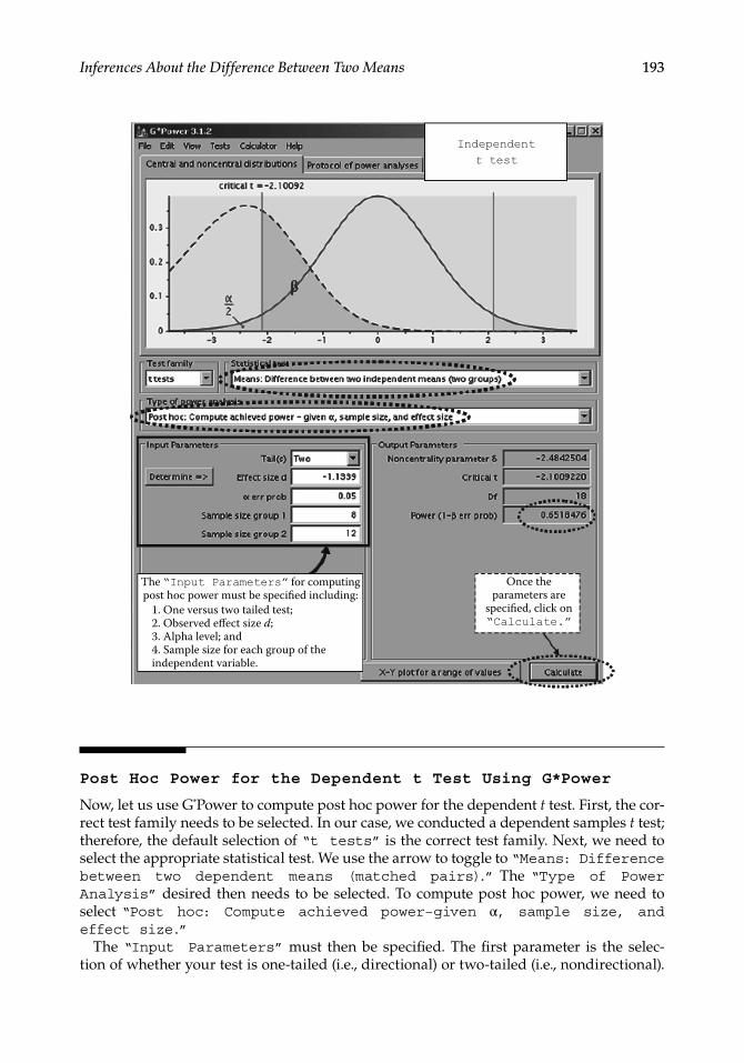
The� first� thing� that� must� be� done� when� using� G*Power� for� computing� post� hoc� power�is� to� select� the� correct� test� family�� In� our� case,� we� conducted� an� independent� samples�t� test;� therefore,� the�default� selection�of�“t tests”� is� the�correct� test� family��Next,�we�need� to� select� the� appropriate� statistical� test�� We� use� the� arrow� to� toggle� to�“Means: Difference between two independent means (two groups).”�The�“Type of Power Analysis”�desired� then�needs� to�be�selected��To�compute�post�hoc�power,�we�need�to�select�“Post hoc: Compute achieved power–given�α, sample size, and effect size.”
The�“Input Parameters”�must�then�be�specified��The�first�parameter�is�the�selection�of�whether�your�test�is�one-tailed�(i�e�,�directional)�or�two-tailed�(i�e�,�nondirectional)��In�this�example,�we�have�a�two-tailed�test�so�we�use�the�arrow�to�toggle�to�“Two.”�The�achieved�or�observed�effect�size�was�−1�1339��The�alpha�level�we�tested�at�was��05,�and�the�sample�size�for�females�was�8�and�for�males,�12��Once�the�parameters�are�specified,�simply�click�on�“Calculate”�to�generate�the�achieved�power�statistics�
The�“Output Parameters”�provide�the�relevant�statistics�given�the�input�just�speci-fied��In�this�example,�we�were�interested�in�determining�post�hoc�power�given�a�two-tailed�test,�with�an�observed�effect�size�of�−1�1339,�an�alpha�level�of��05,�and�sample�sizes�of� 8� (females)� and� 12� (males)�� Based� on� those� criteria,� the� post� hoc� power� was� �65�� In�other�words,�with�a�sample�size�of�8� females�and�12�males� in�our�study,� testing�at�an�alpha�level�of��05�and�observing�a�large�effect�of�−1�1339,�then�the�power�of�our�test�was��65—the�probability�of�rejecting�the�null�hypothesis�when�it�is�really�false�will�be�65%,�which�is�only�moderate�power��Keep�in�mind�that�conducting�power�analysis�a�priori�is�recommended�so�that�you�avoid�a�situation�where,�post�hoc,�you�find�that�the�sample�size�was�not�sufficient�to�reach�the�desired�power�(given�the�observed�effect�size�and�alpha�level)��We�were�fortunate�in�this�example�in�that�we�were�still�able�to�detect�a�statistically�significant�difference�in�cholesterol�levels�between�males�and�females;�however�we�will�likely�not�always�be�that�lucky�
193Inferences About the Difference Between Two Means
The “Input Parameters” for computingpost hoc power must be specified including:
Once theparameters are
specified, click on“Calculate.”
Independent
t test
1. One versus two tailed test;2. Observed effect size d;3. Alpha level; and4. Sample size for each group of theindependent variable.
Post Hoc Power for the Dependent t Test Using G*Power
Now,�let�us�use�G*Power�to�compute�post�hoc�power�for�the�dependent�t�test��First,�the�cor-rect�test�family�needs�to�be�selected��In�our�case,�we�conducted�a�dependent�samples�t�test;�therefore,�the�default�selection�of�“t tests”�is�the�correct�test�family��Next,�we�need�to�select�the�appropriate�statistical�test��We�use�the�arrow�to�toggle�to�“Means: Difference between two dependent means (matched pairs).”� The�“Type of Power Analysis”�desired� then�needs� to�be�selected��To�compute�post�hoc�power,�we�need� to�select�“Post hoc: Compute achieved power–given α, sample size, and effect size.”
The�“Input Parameters”� must� then� be� specified�� The� first� parameter� is� the� selec-tion�of�whether�your�test�is�one-tailed�(i�e�,�directional)�or�two-tailed�(i�e�,�nondirectional)��

194 An Introduction to Statistical Concepts
In�this�example,�we�have�a�two-tailed�test,�so�we�use�the�arrow�to�toggle�to�“Two.”�The�achieved�or�observed�effect�size�was�2�3146��The�alpha�level�we�tested�at�was��05,�and�the�total�sample�size�was�10��Once�the�parameters�are�specified,�simply�click�on�“Calculate”�to�generate�the�achieved�power�statistics�
The�“Output Parameters”�provide�the�relevant�statistics�given�the�input�specified��In�this�example,�we�were�interested�in�determining�post�hoc�power�given�a�two-tailed�test,�with�an�observed�effect�size�of�2�3146,�an�alpha�level�of� �05,�and�total�sample�size�of�10��Based�on�those�criteria,�the�post�hoc�power�was��99��In�other�words,�with�a�total�sample�size�of�10,�testing�at�an�alpha�level�of��05�and�observing�a�large�effect�of�2�3146,�then�the�power�of�our�test�was�over��99—the�probability�of�rejecting�the�null�hypothesis�when�it�is�really�false�will�be�greater�than�99%,�about�the�strongest�power�that�can�be�achieved��Again,�con-ducting�power�analysis�a�priori�is�recommended�so�that�you�avoid�a�situation�where,�post�hoc,�you�find�that�the�sample�size�was�not�sufficient�to�reach�the�desired�power�(given�the�observed�effect�size�and�alpha�level)�
Once theparameters are
specified, click on“Calculate.”
Dependent
t test
�e “Input Parameters” for computingpost hoc power must be specified including:
1. One versus two tailed test;2. Observed effect size d;3. Alpha level; and4. Sample size for each group of the independent variable.
195Inferences About the Difference Between Two Means
7.6 TemplateandAPA-StyleWrite-Up
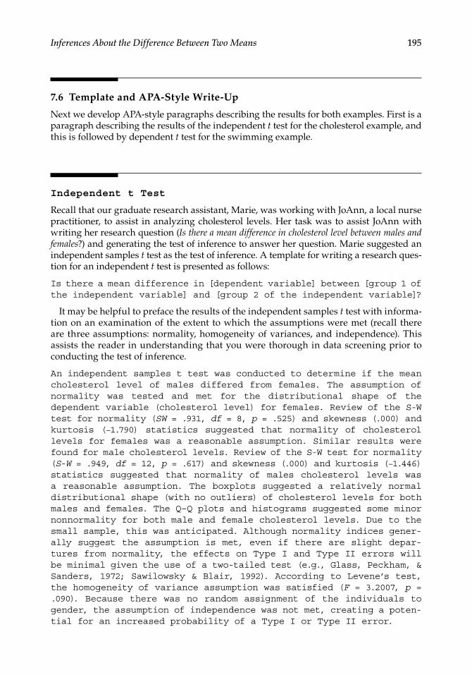
Next�we�develop�APA-style�paragraphs�describing�the�results�for�both�examples��First�is�a�paragraph�describing�the�results�of�the�independent�t�test�for�the�cholesterol�example,�and�this�is�followed�by�dependent�t�test�for�the�swimming�example�
Independent t Test
Recall�that�our�graduate�research�assistant,�Marie,�was�working�with�JoAnn,�a�local�nurse�practitioner,� to�assist� in�analyzing�cholesterol� levels��Her� task�was� to�assist� JoAnn�with�writing�her�research�question�(Is there a mean difference in cholesterol level between males and females?)�and�generating�the�test�of�inference�to�answer�her�question��Marie�suggested�an�independent�samples�t�test�as�the�test�of�inference��A�template�for�writing�a�research�ques-tion�for�an�independent�t�test�is�presented�as�follows:
Is there a mean difference in [dependent variable] between [group 1 of the independent variable] and [group 2 of the independent variable]?
It�may�be�helpful�to�preface�the�results�of�the�independent�samples�t�test�with�informa-tion�on�an�examination�of� the�extent�to�which�the�assumptions�were�met�(recall� there�are� three�assumptions:�normality,�homogeneity�of�variances,�and� independence)��This�assists�the�reader�in�understanding�that�you�were�thorough�in�data�screening�prior�to�conducting�the�test�of�inference�
An independent samples t test was conducted to determine if the mean cholesterol level of males differed from females. The assumption of normality was tested and met for the distributional shape of the dependent variable (cholesterol level) for females. Review of the S-W test for normality (SW = .931, df = 8, p = .525) and skewness (.000) and kurtosis (−1.790) statistics suggested that normality of cholesterol levels for females was a reasonable assumption. Similar results were found for male cholesterol levels. Review of the S-W test for normality (S-W = .949, df = 12, p = .617) and skewness (.000) and kurtosis (−1.446) statistics suggested that normality of males cholesterol levels was a reasonable assumption. The boxplots suggested a relatively normal distributional shape (with no outliers) of cholesterol levels for both males and females. The Q–Q plots and histograms suggested some minor nonnormality for both male and female cholesterol levels. Due to the small sample, this was anticipated. Although normality indices gener-ally suggest the assumption is met, even if there are slight depar-tures from normality, the effects on Type I and Type II errors will be minimal given the use of a two-tailed test (e.g., Glass, Peckham, & Sanders, 1972; Sawilowsky & Blair, 1992). According to Levene’s test, the homogeneity of variance assumption was satisfied (F = 3.2007, p = .090). Because there was no random assignment of the individuals to gender, the assumption of independence was not met, creating a poten-tial for an increased probability of a Type I or Type II error.

196 An Introduction to Statistical Concepts
It�is�also�desirable�to�include�a�measure�of�effect�size��Recall�our�formula�for�computing�the�effect�size,�d,�presented�earlier�in�the�chapter��Plugging�in�the�values�for�our�cholesterol�example,� we� find� an� effect� size� d� of� −1�1339,� which� is� interpreted� according� to� Cohen’s�(1988)�guidelines�as�a�large�effect:
�d
Y Ysp
= − = − = −1 2 185 21526 4575
1 1339.
.
Remember�that�for�the�two-sample�mean�test,�d�indicates�how�many�standard�deviations�the�mean�of�sample�1�is�from�the�mean�of�sample�2��Thus,�with�an�effect�size�of�−1�1339,�there�are�nearly�one�and�one-quarter�standard�deviation�units�between�the�mean�choles-terol�levels�of�males�as�compared�to�females��The�negative�sign�simply�indicates�that�group�1�has�the�smaller�mean�(as�it�is�the�first�value�in�the�numerator�of�the�formula;�in�our�case,�the�mean�cholesterol�level�of�females)�
Here�is�an�APA-style�example�paragraph�of�results�for�the�cholesterol�level�data�(remem-ber�that�this�will�be�prefaced�by�the�paragraph�reporting�the�extent�to�which�the�assump-tions�of�the�test�were�met)�
As shown in Table 7.3, cholesterol data were gathered from samples of 12 males and 8 females, with a female sample mean of 185 (SD = 19.09) and a male sample mean of 215 (SD = 30.22). The independent t test indi-cated that the cholesterol means were statistically significantly dif-ferent for males and females (t = −2.4842, df = 18, p = .023). Thus, the null hypothesis that the cholesterol means were the same by gender was rejected at the .05 level of significance. The effect size d (calculated using the pooled standard deviation) was −1.1339. Using Cohen’s (1988) guidelines, this is interpreted as a large effect. The results provide evidence to support the conclusion that males and females differ in cholesterol levels, on average. More specifically, males were observed to have larger cholesterol levels, on average, than females.
Parenthetically,�notice�that�the�results�of�the�Welch�t′�test�were�the�same�as�for�the�inde-pendent� t� test� (Welch� t′� =� −2�7197,� rounded� df� =� 18,� p� =� �014)�� Thus,� any� deviation� from�homogeneity�of�variance�did�not�affect�the�results�
Dependent t Test
Marie,�as�you�recall,�was�also�working�with�Mark,�a�local�swimming�coach,�to�assist�in�analyz-ing�freestyle�swimming�time�before�and�after�swimmers�participated�in�an�intensive�training�program��Marie�suggested�a�research�question�(Is there a mean difference in swim time for the 50-meter freestyle event before participation in an intensive training program as compared to swim time for the 50-meter freestyle event after participation in an intensive training program?)�and�assisted�in�generating�the�test�of�inference�(specifically�the�dependent�t�test)�to�answer�her�question��A�template�for�writing�a�research�question�for�a�dependent�t�test�is�presented�as�follows�
Is there a mean difference in [paired sample 1] as compared to [paired sample 2]?

197Inferences About the Difference Between Two Means
It�may�be�helpful�to�preface�the�results�of�the�dependent�samples�t�test�with�information�on�the�extent�to�which�the�assumptions�were�met�(recall�there�are�three�assumptions:�normal-ity,�homogeneity�of�variance,�and�independence)��This�assists�the�reader�in�understanding�that�you�were�thorough�in�data�screening�prior�to�conducting�the�test�of�inference�
A dependent samples t test was conducted to determine if there was a difference in the mean swim time for the 50 meter freestyle before participation in an intensive training program as compared to the mean swim time for the 50 meter freestyle after participation in an intensive training program. The assumption of normality was tested and met for the distributional shape of the paired differences. Review of the S-W test for normality (SW = .956, df = 10, p = .734) and skew-ness (.248) and kurtosis (.050) statistics suggested that normality of the paired differences was reasonable. The boxplot suggested a rela-tively normal distributional shape, and there were no outliers pres-ent. The Q–Q plot and histogram suggested minor nonnormality. Due to the small sample, this was anticipated. Homogeneity of variance was tested by reviewing the ratio of the raw score variances. The ratio of the smallest (posttest = 13.111) to largest (pretest = 17.778) variance was less than 1:4; therefore, there is evidence of the equal variance assumption. The individuals were not randomly selected; therefore, the assumption of independence was not met, creating a potential for an increased probability of a Type I or Type II error.
It�is�also�important�to�include�a�measure�of�effect�size��Recall�our�formula�for�computing�the�effect�size,�d,�presented�earlier�in�the�chapter��Plugging�in�the�values�for�our�swimming�example,�we�find�an�effect�size�d�of�2�3146,�which�is�interpreted�according�to�Cohen’s�(1988)�guidelines�as�a�large�effect:
�Cohen d
dsd
= = =52 1602
2 3146.
.
With� an� effect� size� of� 2�3146,� there� are� about� two� and� a� third� standard� deviation� units�between�the�pretraining�mean�swim�time�and�the�posttraining�mean�swim�time�
Here�is�an�APA-style�example�paragraph�of�results�for�the�swimming�data�(remember�that�this�will�be�prefaced�by�the�paragraph�reporting�the�extent�to�which�the�assumptions�of�the�test�were�met)�
From Table 7.4, we see that pretest and posttest data were collected from a sample of 10 swimmers, with a pretest mean of 64 seconds (SD = 4.22) and a posttest mean of 59 seconds (SD = 3.62). Thus, swimming times decreased from pretest to posttest. The dependent t test was conducted to determine if this difference was statistically significantly dif-ferent from 0, and the results indicate that the pretest and posttest means were statistically different (t = 7.319, df = 9, p < .001). Thus, the null hypothesis that the freestyle swimming means were the same at both points in time was rejected at the .05 level of significance. The effect size d (calculated as the mean difference divided by the standard

198 An Introduction to Statistical Concepts
deviation of the difference) was 2.3146. Using Cohen’s (1988) guidelines, this is interpreted as a large effect. The results provide evidence to support the conclusion that the mean 50 meter freestyle swimming time prior to intensive training is different than the mean 50 meter free-style swimming time after intensive training.
7.7 Summary
In�this�chapter,�we�considered�a�second�inferential�testing�situation,�testing�hypotheses�about� the� difference� between� two� means�� Several� inferential� tests� and� new� concepts�were�discussed��New�concepts�introduced�were�independent�versus�dependent�samples,�the�sampling�distribution�of� the�difference�between�two�means,� the�standard�error�of�the�difference�between�two�means,�and�parametric�versus�nonparametric�tests��We�then�moved�on�to�describe�the�following�three�inferential�tests�for�determining�the�difference�between�two�independent�means:�the�independent�t�test,�the�Welch�t′�test,�and�briefly�the�Mann–Whitney–Wilcoxon�test��The�following�two�tests�for�determining�the�differ-ence�between�two�dependent�means�were�considered:�the�dependent�t�test�and�briefly�the�Wilcoxon�signed�ranks�test��In�addition,�examples�were�presented�for�each�of�the�t�tests,�and�recommendations�were�made�as�to�when�each�test� is�most�appropriate��The�chapter�concluded�with�a�look�at�SPSS�and�G*Power�(for�post�hoc�power)�as�well�as�devel-oping�an�APA-style�write-up�of�results��At�this�point,�you�should�have�met�the�following�objectives:�(a)�be�able�to�understand�the�basic�concepts�underlying�the�inferential�tests�of�two�means,�(b)�be�able�to�select�the�appropriate�test,�and�(c)�be�able�to�determine�and�interpret�the�results�from�the�appropriate�test��In�the�next�chapter,�we�discuss�inferential�tests�involving�proportions��Other�inferential�tests�are�covered�in�subsequent�chapters�
Problems
Conceptual problems
7.1� We�test�the�following�hypothesis:
� H0 1 2 0: µ µ− =
� H1 1 2 0: µ µ− ≠
� The�level�of�significance�is��05�and�H0�is�rejected��Assuming�all�assumptions�are�met�and�H0�is�true,�the�probability�of�committing�a�Type�I�error�is�which�one�of�the�following?
� a�� 0� b�� 0�05� c�� Between��05�and��95� d�� 0�95� e�� 1�00

199Inferences About the Difference Between Two Means
7.2� When�H0�is�true,�the�difference�between�two�independent�sample�means�is�a�func-tion�of�which�one�of�the�following?
� a�� Degrees�of�freedom� b�� The�standard�error� c�� The�sampling�distribution� d�� Sampling�error7.3� The�denominator�of�the�independent�t�test�is�known�as�the�standard�error�of�the�
difference�between�two�means,�and�may�be�defined�as�which�one�of�the�following?� a�� The�difference�between�the�two�group�means� b�� The�amount�by�which�the�difference�between�the�two�group�means�differs�from�
the�population�mean� c�� The�standard�deviation�of� the�sampling�distribution�of� the�difference�between�
two�means� d�� All�of�the�above� e�� None�of�the�above7.4� In�the�independent�t�test,�the�homoscedasticity�assumption�states�what?� a�� The�two�population�means�are�equal�� b�� The�two�population�variances�are�equal�� c�� The�two�sample�means�are�equal�� d�� The�two�sample�variances�are�equal�7.5� Sampling�error�increases�with�larger�samples��True�or�false?7.6� At� a� given� level� of� significance,� it� is� possible� that� the� significance� test� and� the� CI�
results�will�differ�for�the�same�dataset��True�or�false?7.7� I�assert�that�the�critical�value�of�t�required�for�statistical�significance�is�smaller�(in�
absolute�value�or�ignoring�the�sign)�when�using�a�directional�rather�than�a�nondirec-tional�test��Am�I�correct?
7.8� If�a�95%�CI�from�an�independent�t�test�ranges�from�−�13�to�+1�67,�I�assert�that�the�null�hypothesis�would�not�be�rejected�at�the��05�level�of�significance��Am�I�correct?
7.9� A�group�of�15�females�was�compared�to�a�group�of�25�males�with�respect�to�intel-ligence��To�test�if�the�sample�sizes�are�significantly�different,�which�of�the�following�tests�would�you�use?
� a�� Independent�t�test� b�� Dependent�t�test� c�� z�test� d�� None�of�the�above7.10� The�mathematic�ability�of�10�preschool�children�was�measured�when�they�entered�
their�first�year�of�preschool�and�then�again�in�the�spring�of�their�kindergarten�year��To�test�for�pre-�to�post-mean�differences,�which�of�the�following�tests�would�be�used?
� a�� Independent�t�test� b�� Dependent�t�test� c�� z�test� d�� None�of�the�above

200 An Introduction to Statistical Concepts
7.11� A� researcher� collected� data� to� answer� the� following� research� question:� Are� there�mean�differences�in�science�test�scores�for�middle�school�students�who�participate�in�school-sponsored�athletics�as�compared�to�students�who�do�not�participate?�Which�of�the�following�tests�would�be�used�to�answer�this�question?
� a�� Independent�t�test� b�� Dependent�t�test� c�� z�test� d�� None�of�the�above7.12� The�number�of�degrees�of�freedom�for�an�independent�t�test�with�15�females�and�
25�males�is�40��True�or�false?7.13� I�assert�that�the�critical�value�of�t,�for�a�test�of�two�dependent�means,�will�increase�as�
the�samples�become�larger��Am�I�correct?7.14� Which�of�the�following�is�NOT�an�assumption�of�the�independent�t�test?� a�� Normality� b�� Independence� c�� Equal�sample�sizes� d�� Homogeneity�of�variance7.15� For�which�of�the�following�assumptions�of�the�independent�t� test� is�evidence�pro-
vided�in�the�SPSS�output�by�default?� a�� Normality� b�� Independence� c�� Equal�sample�sizes� d�� Homogeneity�of�variance
Computational problems
7.1� The�following�two�independent�samples�of�older�and�younger�adults�were�measured�on�an�attitude�toward�violence�test:
Sample1(OlderAdult)Data Sample1(YoungerAdult)Data
42 36 47 45 50 5735 46 37 58 43 5252 44 47 43 60 4151 56 54 49 44 5155 50 40 49� 55� 5640 46 41
� a�� Test�the�following�hypotheses�at�the��05�level�of�significance:
� H0 1 2 0: µ µ− =
� H1 1 2 0: µ µ− ≠
� b�� Construct�a�95%�CI�

201Inferences About the Difference Between Two Means
7.2� The�following�two�independent�samples�of�male�and�female�undergraduate�students�were�measured�on�an�English�literature�quiz:
Sample1(Male)Data Sample1(Female)Data
5 7 8 9 9 1110 11 11 13 15 1813 15 19 20
� a�� Test�the�following�hypotheses�at�the��05�level�of�significance:
� H0 1 2 0: µ µ− =
� H1 1 2 0: µ µ− ≠
� b�� Construct�a�95%�CI�7.3� The� following� two� independent� samples� of� preschool� children� (who� were� demo-
graphically� similar� but� differed� in� Head� Start� participation)� were� measured� on�teacher-reported�social�skills�during�the�spring�of�kindergarten:
Sample1(HeadStart)Data Sample1(Non-HeadStart)Data
18 14 12 15 12 916 10 17 10 18 1220 16 19 11 8 1115 13 22 13 10 14
� a�� Test�the�following�hypothesis�at�the��05�level�of�significance:
� H0 1 2 0: µ µ− =
� H1 1 2 0: µ µ− ≠
� b�� Construct�a�95%�CI�
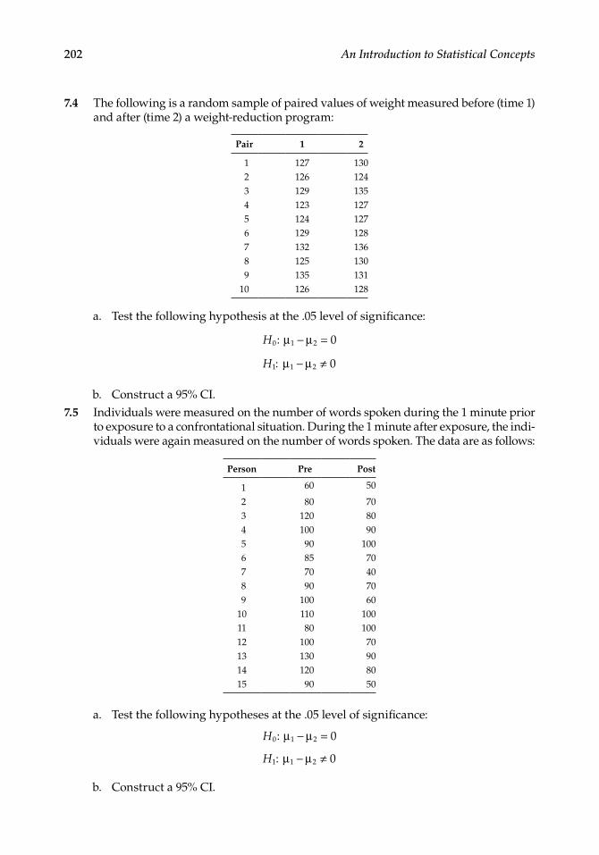
202 An Introduction to Statistical Concepts
7.4� The�following�is�a�random�sample�of�paired�values�of�weight�measured�before�(time�1)�and�after�(time�2)�a�weight-reduction�program:
Pair 1 2
1 127 1302 126 1243 129 1354 123 1275 124 1276 129 1287 132 1368 125 1309 135 131
10 126 128
� a�� Test�the�following�hypothesis�at�the��05�level�of�significance:
� H0 1 2 0: µ µ− =
� H1 1 2 0: µ µ− ≠
� b�� Construct�a�95%�CI�7.5� Individuals�were�measured�on�the�number�of�words�spoken�during�the�1�minute�prior�
to�exposure�to�a�confrontational�situation��During�the�1�minute�after�exposure,�the�indi-viduals�were�again�measured�on�the�number�of�words�spoken��The�data�are�as�follows:
Person Pre Post
1 60 50
2 80 703 120 804 100 905 90 1006 85 707 70 408 90 709 100 60
10 110 10011 80 10012 100 7013 130 9014 120 8015 90 50
� a�� Test�the�following�hypotheses�at�the��05�level�of�significance:
� H0 1 2 0: µ µ− =
� H1 1 2 0: µ µ− ≠
� b�� Construct�a�95%�CI�

203Inferences About the Difference Between Two Means
7.6� The�following�is�a�random�sample�of�scores�on�an�attitude�toward�abortion�scale�for�husband�(sample�1)�and�wife�(sample�2)�pairs:
Pair 1 2
1 1 32 2 33 4 64 4 55 5 76 7 87 7 98 8 10
� a�� Test�the�following�hypotheses�at�the��05�level�of�significance:
� H0 1 2 0: µ µ− =
� H1 1 2 0: µ µ− ≠
� b�� Construct�a�95%�CI�7.7� For� two� dependent� samples,� test� the� following� hypothesis� at� the� �05� level� of�
significance:� Sample�statistics:�n�=�121;�d
–�=�10;�sd�=�45�
� H0 1 2 0: µ µ− =
� H1 1 2 0: µ µ− >
7.8� For� two� dependent� samples,� test� the� following� hypothesis� at� the� �05� level� of�significance�
� Sample�statistics:�n�=�25;�d–�=�25;�sd�=�14�
� H0 1 2 0: µ µ− =
� H1 1 2 0: µ µ− >
Interpretive problems
7.1� Using�the�survey�1�dataset�from�the�website,�use�SPSS�to�conduct�an�independent�t�test,�where�gender�is�the�grouping�variable�and�the�dependent�variable�is�a�vari-able�of�interest�to�you��Test�for�the�extent�to�which�the�assumptions�have�been�met��Calculate�an�effect� size�as�well�as�post�hoc�power��Then�write�an�APA-style�para-graph�describing�the�results�
7.2� Using�the�survey�1�dataset�from�the�website,�use�SPSS�to�conduct�an�independent�t test,�where� the� grouping� variable� is� whether� or� not� the� person� could� tell� the� difference�between�Pepsi�and�Coke�and�the�dependent�variable�is�a�variable�of�interest�to�you��Test�for�the�extent�to�which�the�assumptions�have�been�met��Calculate�an�effect�size�as�well�as�post�hoc�power��Then�write�an�APA-style�paragraph�describing�the�results�