Inference under Covariate-Adaptive Randomization∗

Federico A. Bugni

Department of Economics

Duke University

federico.bugni@duke.edu

Ivan A. Canay

Department of Economics

Northwestern University

iacanay@northwestern.edu

Azeem M. Shaikh

Department of Economics

University of Chicago

amshaikh@uchicago.edu

May 19, 2017

∗We would like to thank the Co-Editor, the Associate Editor, and three anonymous referees for useful comments andsuggestions. We additionally thank Lori Beaman, Robert Garlick, Raymond Guiteras, Aprajit Mahajan, Joseph Romano,Andres Santos, and seminar participants at various institutions for helpful comments on this paper. We finally thank YuehaoBai and Winnie van Dijk for excellent research assistance. The research of the first author was supported by National Institutesof Health Grant 40-4153-00-0-85-399. The research of the second author was supported by National Science Foundation GrantSES-1530534. The research of the third author was supported by National Science Foundation Grants DMS-1308260, SES-1227091, and SES-1530661.

1

Abstract

This paper studies inference for the average treatment effect in randomized controlled trials with

covariate-adaptive randomization. Here, by covariate-adaptive randomization, we mean randomization

schemes that first stratify according to baseline covariates and then assign treatment status so as to

achieve “balance” within each stratum. Our main requirement is that the randomization scheme assigns

treatment status within each stratum so that the fraction of units being assigned to treatment within

each stratum has a well behaved distribution centered around a proportion π as the sample size tends to

infinity. Such schemes include, for example, Efron’s biased-coin design and stratified block randomization.

When testing the null hypothesis that the average treatment effect equals a pre-specified value in such

settings, we first show the usual two-sample t-test is conservative in the sense that it has limiting rejection

probability under the null hypothesis no greater than and typically strictly less than the nominal level.

We show, however, that a simple adjustment to the usual standard error of the two-sample t-test leads

to a test that is exact in the sense that its limiting rejection probability under the null hypothesis equals

the nominal level. Next, we consider the usual t-test (on the coefficient on treatment assignment) in a

linear regression of outcomes on treatment assignment and indicators for each of the strata. We show

that this test is exact for the important special case of randomization schemes with π = 12, but is

otherwise conservative. We again provide a simple adjustment to the standard error that yields an exact

test more generally. Finally, we study the behavior of a modified version of a permutation test, which

we refer to as the covariate-adaptive permutation test, that only permutes treatment status for units

within the same stratum. When applied to the usual two-sample t-statistic, we show that this test is

exact for randomization schemes with π = 12

and that additionally achieve what we refer to as “strong

balance.” For randomization schemes with π 6= 12, this test may have limiting rejection probability under

the null hypothesis strictly greater than the nominal level. When applied to a suitably adjusted version

of the two-sample t-statistic, however, we show that this test is exact for all randomization schemes

that achieve “strong balance,” including those with π 6= 12. A simulation study confirms the practical

relevance of our theoretical results. We conclude with recommendations for empirical practice and an

empirical illustration.

KEYWORDS: Covariate-adaptive randomization, stratified block randomization, Efron’s biased-coin design,

treatment assignment, randomized controlled trial, permutation test, two-sample t-test, strata fixed effects

JEL classification codes: C12, C14

1 Introduction

This paper studies inference for the average treatment effect in randomized controlled trials with covariate-

adaptive randomization. Here, by covariate-adaptive randomization, we mean randomization schemes that

first stratify according to baseline covariates and then assign treatment status so as to achieve “balance”

within each stratum. Many such methods are used routinely when assigning treatment status in randomized

controlled trials in all parts of the sciences. See, for example, Rosenberger and Lachin (2016) for a textbook

treatment focused on clinical trials and Duflo et al. (2007) and Bruhn and McKenzie (2008) for reviews

focused on development economics. In this paper, we take as given the use of such a treatment assignment

mechanism and study its consequences for testing the null hypothesis that the average treatment effect

equals a pre-specified value in such settings. Our main requirement is that the randomization scheme assigns

treatment status within each stratum so that the fraction of units being assigned to treatment within each

stratum has a well behaved distribution centered around a proportion π as the sample size tends to infinity.

Importantly, as explained in Section 3 below, our results apply to most commonly used treatment assignment

mechanisms, including simple random sampling, Efron’s biased coin design, Wei’s adaptive biased coin design,

and stratified block randomization. The latter treatment assignment scheme is especially noteworthy because

of its widespread use recently in development economics. See, for example, Dizon-Ross (2014, footnote 13),

Duflo et al. (2014, footnote 6), Callen et al. (2015, page 24), and Berry et al. (2015, page 6). A caveat to our

analysis, however, is that we require the proportion π to be constant across the strata. For an analysis of

settings where π is allowed to vary across strata, see Imbens and Rubin (2015, Chapter 9) and Bugni et al.

(2016).

Our first result establishes that the usual two-sample t-test is conservative in the sense that it has limiting

rejection probability under the null hypothesis no greater than and typically strictly less than the nominal

level. We additionally provide a characterization of when the limiting rejection probability under the null

hypothesis is in fact strictly less than the nominal level. As explained further in Remark 4.3 below, our result

substantially generalizes a related result obtained by Shao et al. (2010), who established this phenomenon

under much stronger assumptions and for only one specific randomization scheme. In a simulation study, we

find that the rejection probability of these tests may in fact be dramatically less than the nominal level, and,

as a result, they may have very poor power when compared to other tests. Intuitively, the conservative feature

of these tests is a consequence of the dependence in treatment status across units and between treatment

status and baseline covariates resulting from covariate-adaptive randomization. We show, however, that a

simple adjustment to the usual standard error of the two-sample t-test leads to a test that is exact in the

sense that its limiting rejection probability under the null hypothesis equals the nominal level.

Next, we consider the usual t-test (on the coefficient on treatment assignment) in a linear regression of

outcomes on treatment assignment and indicators for each of the strata. We refer to this test as the t-test

with strata fixed effects. Based on simulation evidence and earlier assertions by Kernan et al. (1999), the

use of this test has been recommended by Bruhn and McKenzie (2008), but, to the best of our knowledge,

there has not yet been any formal analysis of its properties. Our results show that this test is typically

conservative as well. As in the case of the two-sample t-test, we additionally provide a characterization of

when the limiting rejection probability under the null hypothesis is in fact strictly less than the nominal

level. This characterization reveals that the test is exact for the the important special case of randomization

1

schemes with π = 12 . We again provide a simple adjustment to the standard errors that yields an exact test

more generally.

Finally, we study the behavior of a modified version of a permutation test, which we refer to as the

covariate-adaptive permutation test, that only permutes treatment status for units within the same stratum.

When applied to the usual two-sample t-statistic, we show that this test is exact for randomization schemes

with π = 12 and that additionally achieve what we refer to as “strong balance,” defined formally in Section

2 below. For randomization schemes with π 6= 12 , this test may have limiting rejection probability under the

null hypothesis strictly greater than the nominal level. When applied to a suitably adjusted version of the

two-sample t-statistic, however, we show that this test is exact for all randomization schemes that achieve

“strong balance,” including those with π 6= 12 . As explained further in Remark 4.11 below, this test or closely

related tests have been previously proposed and justified in finite samples for testing much more narrowly

defined versions of the null hypothesis, including what is sometimes referred to as the “sharp null hypothesis.”

See, for example, Rosenbaum (2007), Heckman et al. (2011), Lee and Shaikh (2014), Rosenberger and Lachin

(2016, Section 6.4), and, more recently, Young (2016). Exploiting recent results on the large-sample behavior

of permutation tests by Chung and Romano (2013), our results, in contrast, asymptotically justify the use

of the covariate-adaptive permutation test for testing the null hypothesis that the average treatment effect

equals a pre-specified value for randomization schemes satisfying our assumptions below, while retaining in

some cases the finite-sample validity for the narrower version of the null hypothesis.

The remainder of the paper is organized as follows. In Section 2, we describe our setup and notation.

In particular, there we describe the assumptions we impose on the treatment assignment mechanism and

what we mean by randomization schemes that achieve “strong balance.” In Section 3, we discuss several

examples of treatment assignment mechanisms satisfying these assumptions. Our main results concerning

the two-sample t-test, the t-test with strata fixed effects, and the covariate-adaptive permutation test are

contained in Section 4. In Section 5, we examine the finite-sample behavior of these tests as well as some

other tests via a small simulation study. We discuss recommendations for empirical practice based on our

theoretical results in Section 6. Finally, in Section 7, we provide an empirical illustration of our methods.

Proofs of all results are provided in the Appendix.

2 Setup and Notation

Let Yi denote the (observed) outcome of interest for the ith unit, Ai denote an indicator for whether the

ith unit is treated or not, and Zi denote observed, baseline covariates for the ith unit. Further denote by

Yi(1) the potential outcome of the ith unit if treated and by Yi(0) the potential outcome of the ith unit if

not treated. As usual, the (observed) outcome and potential outcomes are related to treatment assignment

by the relationship

Yi = Yi(1)Ai + Yi(0)(1−Ai) . (1)

Denote by Pn the distribution of the observed data

X(n) = (Yi, Ai, Zi) : 1 ≤ i ≤ n

2

and denote by Qn the distribution of

W (n) = (Yi(1), Yi(0), Zi) : 1 ≤ i ≤ n .

Note that Pn is jointly determined by (1), Qn, and the treatment assignment mechanism. We therefore

state our assumptions below in terms of assumptions on Qn and assumptions on the treatment assignment

mechanism. Indeed, we will not make reference to Pn in the sequel and all operations are understood to be

under Qn and the treatment assignment mechanism.

Strata are constructed from the observed, baseline covariates Zi using a function S : supp(Zi) → S,

where S is a finite set. For 1 ≤ i ≤ n, let Si = S(Zi) and denote by S(n) the vector of strata (S1, . . . , Sn).

We begin by describing our assumptions on Qn. We assume that W (n) consists of n i.i.d. observations,

i.e., Qn = Qn, where Q is the marginal distribution of (Yi(1), Yi(0), Zi). We further restrict Q to satisfy the

following mild requirement:

Assumption 2.1. Q satisfies

E[Y 2i (1)] <∞ and E[Y 2

i (0)] <∞

and

min

Var[Yi(0)− E[Yi(0)|Si]],Var[Yi(1)− E[Yi(1)|Si]]> 0 .

We note that the second requirement in Assumption 2.1 is made only to rule out degenerate situations and

is stronger than required for our results.

Next, we describe our assumptions on the mechanism determining treatment assignment. In order to

describe these assumptions more formally, we require some further notation. To this end, denote by A(n)

the vector of treatment assignments (A1, . . . , An) and, for s ∈ S, let

Dn(s) =∑

1≤i≤n

(Ai − π)ISi = s , (2)

where π ∈ (0, 1) is the “target” proportion of units to assign to treatment in each stratum. Note that Dn(s)

as defined in (2) measures the amount of imbalance in stratum s relative to this “target” proportion. In

order to rule out trivial strata, we henceforth assume that p(s) = PSi = s > 0 for all s ∈ S. Our other

requirements on the treatment assignment mechanism are summarized in the following assumption:

Assumption 2.2. The treatment assignment mechanism is such that

(a) W (n) ⊥⊥ A(n)|S(n),

(b)

Dn(s)√

n

s∈S

∣∣∣S(n)

d→ N(0,ΣD) a.s., where

ΣD = diagp(s)τ(s) : s ∈ S

with 0 ≤ τ(s) ≤ π(1− π) for all s ∈ S.

3

Assumption 2.2.(a) simply requires that the treatment assignment mechanism is a function only of the

vector of strata and an exogenous randomization device. Assumption 2.2.(b) formalizes our requirement that

the randomization scheme assigns treatment status within each stratum so that the fraction of units being

assigned to treatment within each stratum has a well behaved distribution centered around the “target”

proportion π as the sample size tends to infinity. In the following section, we provide several important

examples of treatment assignment mechanisms satisfying this assumption, including many that are used

routinely in the sciences, including clinical trials and development economics. When Assumption 2.2.(b)

holds with τ(s) = 0 for all s ∈ S, we say that the randomization scheme achieves “strong balance.” This

terminology is intended to reflect the fact that the measure of imbalance Dn(s) is less dispersed around zero

when Assumption 2.2.(b) holds with τ(s) = 0 when compared with the case where it holds with τ(s) > 0.

Our object of interest is the average effect of the treatment on the outcome of interest, defined to be

θ(Q) = E[Yi(1)− Yi(0)] . (3)

For a pre-specified choice of θ0, the testing problem of interest is

H0 : θ(Q) = θ0 versus H1 : θ(Q) 6= θ0 (4)

at level α ∈ (0, 1).

Remark 2.1. The term “balance” is often used in a different way to describe whether the distributions of

baseline covariates Zi in the treatment and control groups are similar. For example, this might be measured

according to the difference in the means of Zi in the treatment and control groups. Our usage follows the

usage in Efron (1971) or Hu and Hu (2012), where “balance” refers to the extent to which the of fraction of

treated units within a strata differs from the target proportion π.

3 Examples

In this section, we briefly describe several different randomization schemes that satisfy our Assumption 2.2.

A more detailed review of these methods and their properties can be found in Rosenberger and Lachin

(2016). In our descriptions, we make use of the notation A(k−1) = (A1, . . . , Ak−1) and S(k) = (S1, . . . , Sk)

for 1 ≤ k ≤ n, where A(0) is understood to be a constant.

Example 3.1. (Simple Random Sampling) Simple random sampling, also known as Bernoulli trials, refers

to the case where A(n) consists of n i.i.d. random variables with

PAk = 1|S(k), A(k−1) = PAk = 1 = π (5)

for 1 ≤ k ≤ n. In this case, Assumption 2.2.(a) follows immediately from (5), and Assumption 2.2.(b) follows

from the central limit theorem with τ(s) = π(1− π) for all s ∈ S. Note that E[Dn(s)] = 0 for all s ∈ S, so

SRS ensures “balance” on average, yet in finite samples Dn(s) may be far from zero.

Example 3.2. (Biased-Coin Design) A biased-coin design is a generalization of simple random sampling

with π = 12 originally proposed by Efron (1971) with the aim of improving “balance” in finite samples. In

4

this randomization scheme, treatment assignment is determined recursively for 1 ≤ k ≤ n as follows:

PAk = 1|S(k), A(k−1) =

12 if Dk−1(Sk) = 0

λ if Dk−1(Sk) < 0

1− λ if Dk−1(Sk) > 0

, (6)

where Dk−1(Sk) =∑

1≤i≤k−1(Ai − 1

2

)ISi = Sk, and 1

2 < λ ≤ 1. Here, D0(S1) is understood to be zero.

The randomization scheme adjusts the probability with which the kth unit is assigned to treatment in an

effort to improve “balance” in the corresponding stratum in finite samples. It follows from Lemma B.11 in

the Appendix that this treatment assignment mechanism satisfies Assumption 2.2 with π = 12 . In particular,

it is an example of a randomization scheme that achieves “strong balance” in that Assumption 2.2.(b) holds

with τ(s) = 0 for all s ∈ S. In this sense, we see that biased-coin design provides improved “balance” relative

to simple random sampling.

Example 3.3. (Adaptive Biased-Coin Design) An adaptive biased-coin design, also known as Wei’s urn

design, is an alternative generalization of simple random sampling with π = 12 originally proposed by Wei

(1978). This randomization scheme is similar to a biased-coin design, except that the probability λ in (6)

depends on Dk−1(Sk) defined in Example 3.2, the magnitude of imbalance among the first k− 1 units in the

corresponding stratum. More precisely, in this randomization scheme, treatment assignment is determined

recursively for 1 ≤ k ≤ n as follows:

PAk = 1|S(k), A(k−1) = ϕ

(Dk−1(Sk)

k − 1

), (7)

where ϕ(x) : [−1, 1] → [0, 1] is a pre-specified non-increasing function satisfying ϕ(−x) = 1 − ϕ(x). Here,D0(S1)

0 is understood to be zero. It follows from Lemma B.12 in the Appendix that this treatment assignment

mechanism satisfies Assumption 2.2 with π = 12 . In particular, Assumption 2.2.(b) holds with τ(s) =

14 (1 − 4ϕ′(0))−1, which lies in the interval (0, 14 ) for the choice of ϕ(x) recommended by Wei (1978) and

used in Section 5. In this sense, adaptive biased-coin designs provide improved “balance” relative to simple

random sampling with π = 12 (i.e., τ(s) < 1

4 ), but to a lesser extent than biased-coin designs (i.e., τ(s) > 0).

Example 3.4. (Stratified Block Randomization) An early discussion of stratified block randomization is

provided by Zelen (1974). This randomization scheme is sometimes also referred to as block randomization

or permuted blocks within strata. In order to describe this treatment assignment mechanism, for s ∈ S,

denote by n(s) the number of units in stratum s and let m(s) ≤ n(s) be given. In this randomization scheme,

m(s) units in stratum s are assigned to treatment and the remainder are assigned to control, where all(n(s)

m(s)

)possible assignments are equally likely and treatment assignment across strata are independent. By setting

m(s) = bπn(s)c , (8)

5

this scheme ensures |Dn(s)| ≤ 1 for all s ∈ S and therefore exhibits the best “balance” in finite samples

among the methods discussed here. It follows from Lemma B.13 in the Appendix that this treatment

assignment mechanism satisfies Assumption 2.2. In particular, as in Example 3.2, it is also an example of a

randomization scheme that achieves “strong balance” in that Assumption 2.2.(b) holds with τ(s) = 0 for all

s ∈ S.

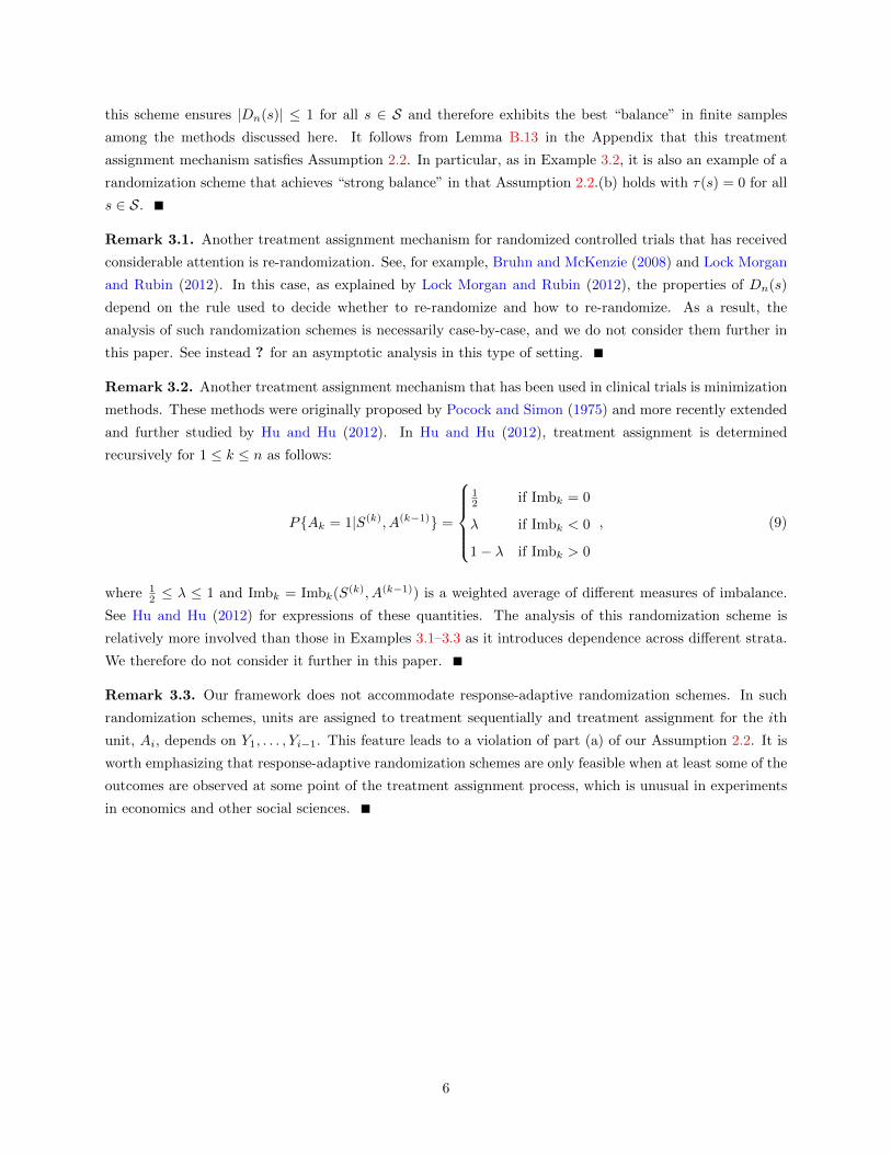
Remark 3.1. Another treatment assignment mechanism for randomized controlled trials that has received

considerable attention is re-randomization. See, for example, Bruhn and McKenzie (2008) and Lock Morgan

and Rubin (2012). In this case, as explained by Lock Morgan and Rubin (2012), the properties of Dn(s)

depend on the rule used to decide whether to re-randomize and how to re-randomize. As a result, the

analysis of such randomization schemes is necessarily case-by-case, and we do not consider them further in

this paper. See instead ? for an asymptotic analysis in this type of setting.

Remark 3.2. Another treatment assignment mechanism that has been used in clinical trials is minimization

methods. These methods were originally proposed by Pocock and Simon (1975) and more recently extended

and further studied by Hu and Hu (2012). In Hu and Hu (2012), treatment assignment is determined

recursively for 1 ≤ k ≤ n as follows:

PAk = 1|S(k), A(k−1) =

12 if Imbk = 0

λ if Imbk < 0

1− λ if Imbk > 0

, (9)

where 12 ≤ λ ≤ 1 and Imbk = Imbk(S(k), A(k−1)) is a weighted average of different measures of imbalance.

See Hu and Hu (2012) for expressions of these quantities. The analysis of this randomization scheme is

relatively more involved than those in Examples 3.1–3.3 as it introduces dependence across different strata.

We therefore do not consider it further in this paper.

Remark 3.3. Our framework does not accommodate response-adaptive randomization schemes. In such

randomization schemes, units are assigned to treatment sequentially and treatment assignment for the ith

unit, Ai, depends on Y1, . . . , Yi−1. This feature leads to a violation of part (a) of our Assumption 2.2. It is

worth emphasizing that response-adaptive randomization schemes are only feasible when at least some of the

outcomes are observed at some point of the treatment assignment process, which is unusual in experiments

in economics and other social sciences.

6

4 Main Results

4.1 Two-Sample t-Test

In this section, we consider using the two-sample t-test to test (4) at level α ∈ (0, 1). In order to define this

test, for a ∈ 0, 1, let

Yn,a =1

na

∑1≤i≤n

YiIAi = a

σ2n,a =

1

na

∑1≤i≤n

(Yi − Yn,a)2IAi = a ,

where na = |1 ≤ i ≤ n : Ai = a|. The two-sample t-test is given by

φt-testn (X(n)) = I|T t-statn (X(n))| > z1−α2 , (10)

where

T t-statn (X(n)) =Yn,1 − Yn,0 − θ0√

σ2n,1

n1+

σ2n,0

n0

(11)

and z1−α2 is the 1 − α2 quantile of a standard normal random variable. This test may equivalently be

described as the usual t-test (on the coefficient on treatment assignment) in a linear regression of outcomes

on treatment assignment with heteroskedasticity-robust standard errors. It is used routinely throughout

economics and the social sciences, including settings with covariate-adaptive randomization (see Duflo et al.

(2007, Section 4), Bruhn and McKenzie (2008, Section E), and references therein). Note that further results

on linear regression are developed in Section 4.2 below.

The following theorem describes the asymptotic behavior of the two-sample t-statistic defined in (11)

and, as a consequence, the two-sample t-test defined in (10) under covariate-adaptive randomization. In

particular, the theorem shows that the limiting rejection probability of the two-sample t-test under the null

hypothesis is generally strictly less than the nominal level.

Theorem 4.1. Suppose Q satisfies Assumption 2.1 and the treatment assignment mechanism satisfies As-

sumption 2.2. Then,Yn,1 − Yn,0 − θ(Q)√

σ2n,1

n1+

σ2n,0

n0

d→ N(0, ς2t-test) ,

where ς2t-test ≤ 1. Furthermore, ς2t-test < 1 unless

(π(1− π)− τ(s))

(1

πE[m1(Zi)|Si = s] +

1

1− πE[m0(Zi)|Si = s]

)2

= 0 for all s ∈ S , (12)

where

ma(Zi) = E[Yi(a)|Zi]− E[Yi(a)] (13)

7

for a ∈ 0, 1. Thus, for the problem of testing (4) at level α ∈ (0, 1), φt-testn (X(n)) defined in (10) satisfies

limn→∞

E[φt-testn (X(n))] = Pςt-test|Z| > z1−α2 ≤ α , (14)

where Z ∼ N(0, 1), whenever Q additionally satisfies the null hypothesis, i.e., θ(Q) = θ0. Furthermore, the

inequality in (14) is strict unless (12) holds.

Remark 4.1. Note that the two-sample t-test defined in (10) uses the 1− α2 quantile of a standard normal

random variable instead of the corresponding quantile of a t-distribution. Theorem 4.1 remains true with

such a choice of critical value. See Imbens and Kolesar (2012) for a recent review of some such degrees of

freedom adjustments.

Remark 4.2. While we generally expect that (12) will fail to hold, there are some important cases in which

it does hold. First, as explained in Example 3.1, for simple random sampling Assumption 2.2 holds with

τ(s) = π(1 − π) for all s ∈ S. Hence, (12) holds, and Theorem 4.1 implies, as one would expect, that the

two-sample t-test is not conservative under simple random sampling. Second, if stratification is irrelevant

for potential outcomes in the sense that E[Yi(a)|Si] = E[Yi(a)] for all a ∈ 0, 1, then E[ma(Zi)|Si] = 0 for

a ∈ 0, 1. Hence, (12) again holds, and Theorem 4.1 implies that the two-sample t-test is not conservative

when stratification is irrelevant for potential outcomes. Note that a special case of irrelevant stratification

is simply no stratification, i.e., Si is constant.

Remark 4.3. Under substantially stronger assumptions than those in Theorem 4.1, Shao et al. (2010) also

establish conservativeness of the two-sample t-test for a specific covariate-adaptive randomization scheme.

For a textbook summary of the results in Shao et al. (2010), see Section 9.5 of Rosenberger and Lachin

(2016). Shao et al. (2010) require, in particular, that ma(Zi) = γ′Zi, that Var[Yi(a)|Zi] does not depend on

Zi, and that the treatment assignment rule is a biased-coin design, as described in Example 3.2. Theorem

4.1 relaxes all of these requirements.

Remark 4.4. While Theorem 4.1 characterizes when the limiting rejection probability of the two-sample

t-test under the null hypothesis is strictly less than the nominal level, it does not reveal how significant this

difference might be. The magnitude of this difference will, of course, depend on the value of ς2t-test, which

will in turn depend on Q and the treatment assignment mechanism. In our simulation study in Section 5,

we find that the rejection probability may in fact be dramatically less than the nominal level and that this

difference translates into substantial power losses when compared with exact tests studied below.

We now provide an adjustment to the two-sample t-test that leads to a test that is exact in the sense that

its limiting rejection probability under the null hypothesis equals the nominal level. In order to describe the

test, we first observe that in the proof of Theorem 4.1 in the Appendix, it is shown that

√n(Yn,1 − Yn,0 − θ(Q))

d→ N(0, ς2Y

(π) + ς2H + ς2A(π)) , (15)

8

where

ς2Y

(π) =1

πVar[Yi(1)] +

1

1− πVar[Yi(0)] (16)

ς2H = E[(E[m1(Zi)|Si]− E[m0(Zi)|Si])2] (17)

ς2A(π) = E

[τ(Si)

(1

πE[m1(Zi)|Si] +

1

1− πE[m0(Zi)|Si]

)2]

(18)

with Yi(a) = Yi(a) − E[Yi(a)|Si] for a ∈ 0, 1. Natural estimators of the quantities in (16)–(18) may be

constructed by replacing population quantities with their sample counterparts. In order to define these

estimators formally, it is useful to introduce some further notation. For a ∈ 0, 1, let

µn,a(s) =1

na(s)

∑1≤i≤n

YiIAi = a, Si = s (19)

where na(s) = |1 ≤ i ≤ n : Ai = a, Si = s|. In terms of this notation, we may define the following

estimators:

ς2Y

(π) =1

π

1

n1

∑1≤i≤n

Y 2i Ai −

∑s∈S

n(s)

nµn,1(s)2

+

1

1− π

1

n0

∑1≤i≤n

Y 2i (1−Ai)−

∑s∈S

n(s)

nµn,0(s)2

(20)

ς2H =∑s∈S

n(s)

n

((µn,1(s)− Yn,1)− (µn,0(s)− Yn,0)

)2(21)

ς2A(π) =∑s∈S

τ(s)n(s)

n

(1

π(µn,1(s)− Yn,1) +

1

1− π(µn,0(s)− Yn,0)

)2

. (22)

In (20)–(22), recall that n(s), as in Example 3.4, denotes the number of units in stratum s. The “adjusted”

two-sample t-test is given by

φt-test,adjn (X(n)) = I|T t-stat,adjn (X(n))| > z1−α2 , (23)

where

T t-stat,adjn (X(n)) =Yn,1 − Yn,0 − θ0√ς2Y(π)+ς2H+ς2A(π)

n

. (24)

The following theorem establishes the desired result about the asymptotic behavior of the “adjusted” two-

sample t-test.

Theorem 4.2. Suppose Q satisfies Assumption 2.1 and the treatment assignment mechanism satisfies As-

sumption 2.2. For the problem of testing (4) at level α ∈ (0, 1), φt-test,adjn (X(n)) defined in (23) satisfies

limn→∞

E[φt-test,adjn (X(n))] = α (25)

whenever Q additionally satisfies the null hypothesis, i.e., θ(Q) = θ0.

9

4.2 t-Test with Strata Fixed Effects

In this section, we consider using the usual t-test (on the coefficient on treatment assignment) in a lin-

ear regression of outcomes on treatment assignment and indicators for each of the strata. As mentioned

previously, we refer to this test as the t-test with strata fixed effects. For concreteness, we use the usual

heteroskedasticity-robust standard errors. Note that the two-sample t-test studied in Section 4.1 can be

viewed as the usual t-test (on the coefficient on treatment assignment) in a linear regression of outcomes on

treatment assignment only with heteroksedasticity-robust standard errors. It follows from Theorem 4.1 and

Remark 4.2 that such a test is conservative in the sense that the limiting rejection probability under the

null hypothesis may be strictly less than the nominal level. In this section, we first show that the addition

of strata fixed effects results in a test is exact in the important special case of randomization schemes with

π = 12 , but remains conservative otherwise.

In order to define the test, consider estimation of the equation

Yi = βAi +∑s∈S

δsISi = s+ ui (26)

by ordinary least squares. Denote by βn the resulting estimator of β in (26). Let

T sfen (X(n)) =

βn − θ0√Vn,βn

, (27)

where Vn,β equals the usual heteroskedasticity-robust standard error for βn. See (A-60) in the Appendix for

an exact expression. Using this notation, the test of interest is given by

φsfen (X(n)) = I|T sfen (X(n))| > z1−α2 . (28)

The following theorem describes the asymptotic behavior of the proposed test. In particular, it shows

that its limiting rejection probability under the null hypothesis equals the nominal level for randomization

schemes with π = 12 and is generally strictly less than the nominal level otherwise.

Theorem 4.3. Suppose Q satisfies Assumption 2.1 and the treatment assignment mechanism satisfies As-

sumption 2.2. Then,

βn − θ0√Vn,βn

d→ N(0, ς2sfe) , (29)

where ς2sfe ≤ 1. Furthermore, ς2sfe < 1 unless

(1− 2π) (π(1− π)− τ(s)) (E[m1(Zi)|Si = s]− E[m0(Zi)|Si = s])2

= 0 for all s ∈ S . (30)

Thus, for the problem of testing (4) at level α ∈ (0, 1), φsfen (X(n)) defined in (28) satisfies

limn→∞

E[φsfen (X(n))] = Pςsfe|Z| > z1−α2 ≤ α (31)

10

where Z ∼ N(0, 1), for Q additionally satisfying the null hypothesis, i.e., θ(Q) = θ0. Furthermore, the

inequality in (31) is strict unless (30) holds.

Remark 4.5. As in the case of the two-sample t-test, we generally expect that (30) will fail to hold, but

there are again some important cases in which it does hold. As one would expect, it again holds in the

case of simple random sampling and when stratification is irrelevant for potential outcomes in the sense that

E[Yi(a)|Si] = E[Yi(a)] for all a ∈ 0, 1, but it additionally holds when π = 12 .

Remark 4.6. In Lemma B.10 in the Appendix, we show that replacing the heteroskedasticity-robust stan-

dard error with the homoskedasticity-only standard error also leads to an exact test when π = 12 . This result

may seem surprising at first, but it may be viewed as a generalization of the following familiar fact in the

usual two-sample t-test: even if the variances in the two samples are different, one may use either the pooled

or unpooled estimate of the variance whenever the ratio of the two sample sizes tends to one. When π 6= 12 ,

however, using the homoskedasticity-only standard error leads to a test whose limiting rejection probability

under the null hypothesis may strictly exceed the nominal level.

Remark 4.7. As in the literature on linear panel data models with fixed effects, βn may be equivalently

computed using ordinary least squares and the deviations of Yi and Ai from their respective means within

strata. However, it is important to note that the resulting standard errors are not equivalent to the usual

heteroksedasticity-robust standard errors associated with ordinary least squares estimation of (26).

As in the case of the two-sample t-test studied previously, it is possible to provide an adjustment to the

t-test with strata fixed effects that leads to a test that is exact. In order to describe the test, we first observe

that in the proof of Theorem 4.3 in the Appendix, it is shown that

√n(βn − θ(Q))

d→ N(0, ς2Y

(π) + ς2H + ς2π) , (32)

where ς2Y

(π) and ς2H are defined as in (16) and (17) and

ς2π =(1− 2π)2

π2(1− π)2E[τ(Si)(E[m1(Zi)|Si]− E[m0(Zi)|Si])2] . (33)

As before, replacing population quantities with their sample counterparts leads to a natural estimator of

(33), specifically,

ς2π =(1− 2π)2

π2(1− π)2

∑s∈S

τ(s)n(s)

n

((µn,1(s)− Yn,1)− (µn,0(s)− Yn,0)

)2, (34)

where µn,a(s) is defined as in (19). The “adjusted” t-test with strata fixed effects is given by

φsfe,adjn (X(n)) = I|T sfe,adjn (X(n))| > z1−α2 , (35)

where

T sfe,adjn (X(n)) =

βn − θ0√ς2Y(π)+ς2H+ς2π

n

(36)

and ς2Y

(π) and ς2H are defined as in (20) and (21). The following theorem establishes the desired result about

11

the asymptotic behavior of the “adjusted” t-test with strata fixed effects.

Theorem 4.4. Suppose Q satisfies Assumption 2.1 and the treatment assignment mechanism satisfies As-

sumption 2.2. For the problem of testing (4) at level α ∈ (0, 1), φsfe,adjn (X(n)) defined in (35) satisfies

limn→∞

E[φsfe,adjn (X(n))] = α (37)

whenever Q additionally satisfies the null hypothesis, i.e., θ(Q) = θ0.

Remark 4.8. In the leading case of randomization schemes that achieve “strong balance,” i.e., satisfying

τ(s) = 0 for all s ∈ S, it is worth emphasizing that the limiting variances in (15) and (32) are identical. In this

sense, there is no reason to prefer one of φt-test,adjn (X(n)) or φsfe,adjn (X(n)) over the other for such randomization

schemes. As explained in Section 3, examples of randomization schemes that achieve “strong balance” include

biased-coin designs and stratified block randomization. More generally, the limiting variances in (15) and

(32) are not ordered unambiguously.

Remark 4.9. Imbens and Rubin (2015, Ch. 9.6) examine the limit in probability of βn under a specific

randomization scheme, namely, stratified block randomization; see Example 3.4. In contrast to our results,

they do not impose the requirement that m(s) is chosen as in (8). In particular, they allow the proportion

π to vary across strata. As a result, Assumption 2.2.(b) does not necessarily hold, and they conclude that

βn is generally not consistent for the average treatment effect, θ(Q). By exploiting Assumption 2.2.(b), we

show that that βn is in fact consistent for θ(Q). Imbens and Rubin (2015, Theorem 9.1) also analyze the

limiting behavior of√n(βn − θ(Q)). While they do not formally study φsfen (X(n)), their expression for the

limiting variance suggests that this test would be exact when m(s) is chosen as in (8). Our results show that

this is generally not the case. In our simulation study in Section 5, we find that the rejection probability

may in fact be dramatically less than the nominal level and that this difference translates into substantial

power loss when compared with exact tests. For further discussion and results for the case of randomization

schemes where the proportion π to vary across strata, see Bugni et al. (2016).

4.3 Covariate-Adaptive Permutation Test

In this section, we study the properties of a modified version of the permutation test, which we term the

covariate-adaptive permutation test. In order to define the test, we require some further notation. Define

Gn(S(n)) = g ∈ Gn : Sg(i) = Si for all 1 ≤ i ≤ n , (38)

i.e., Gn(S(n)) is the subgroup of permutations of n elements that only permutes indices within strata. Define

the action of g ∈ Gn(S(n)) on X(n) as follows:

gX(n) = (Yi, Ag(i), Zi) : 1 ≤ i ≤ n ,

i.e., g ∈ Gn acts on X(n) by permuting treatment assignment. For a given choice of test statistic Tn(X(n)),

the covariate-adaptive permutation test is given by

φcapn (X(n)) = ITn(X(n)) > ccapn (1− α) , (39)

12

where

ccapn (1− α) = inf

x ∈ R :1

|Gn(S(n))|∑

g∈Gn(S(n))

ITn(gX(n)) ≤ x ≥ 1− α

. (40)

The following theorem describes the asymptotic behavior of the covariate-adaptive permutation test

defined in (39) with Tn(X(n)) given by the absolute value of T t-statn (X(n)) in (11). In particular, it shows

that the limiting rejection probability of the proposed test under the null hypothesis equals the nominal level

for randomization schemes with π = 12 and τ(s) = 0 for all s ∈ S. As explained in Section 3, examples of

such randomization schemes include biased-coin designs and stratified block randomization with π = 12 .

Theorem 4.5. Suppose Q satisfies Assumption 2.1 and the treatment assignment mechanism satisfies As-

sumption 2.2 with π = 12 and τ(s) = 0 for all s ∈ S. For the problem of testing (4) at level α ∈ (0, 1),

φcapn (X(n)) defined in (39) with Tn(X(n)) given by the absolute value of T t-statn (X(n)) in (11) satisfies

limn→∞

E[φcapn (X(n))] = α (41)

whenever Q additionally satisfies the null hypothesis, i.e., θ(Q) = θ0.

A by-product of the proof of Theorem 4.5 in the Appendix is that (41) holds even if π 6= 12 provided that

Var[Yi(1)] = Var[Yi(0)] and Var[Yi(1)] = Var[Yi(0)] ,

where Yi(a) = Yi(a) − E[Yi(a)|Si] for a ∈ 0, 1. Outside of this exceptional circumstance, the limiting

rejection probability of the test considered in Theorem 4.5 may strictly exceed the nominal level when π 6= 12 ,

as is evident in our simulation study in Section 5. The following theorem shows that this shortcoming of the

covariate-adaptive permutation test can be removed by applying it with a more suitable choice of Tn(X(n)),

namely the absolute value of T t-stat,adjn (X(n)) in (36). In this way, the theorem highlights the importance

of Studentizing appropriately when applying the covariate-adaptive permutation test. See also Remark 4.13

below.

Theorem 4.6. Suppose Q satisfies Assumption 2.1 and the treatment assignment mechanism satisfies As-

sumption 2.2 with τ(s) = 0 for all s ∈ S. For the problem of testing (4) at level α ∈ (0, 1), φcapn (X(n))

defined in (39) with Tn(X(n)) given by the absolute value of T t-stat,adjn (X(n)) in (24) satisfies

limn→∞

E[φcapn (X(n))] = α

whenever Q additionally satisfies the null hypothesis, i.e., θ(Q) = θ0.

Remark 4.10. Note that Dn(s)/√n : s ∈ S is invariant with respect to transformations g ∈ Gn(S(n)).

For this reason, it is not surprising that the validity of the covariate-adaptive permutation test in Theorems

4.5–4.6 requires that there is no (limiting) variation in this quantity in the sense that τ(s) = 0 for all s ∈ S.

Remark 4.11. By arguing as in Heckman et al. (2011) or Lee and Shaikh (2014), it is possible to show that

(39) with any choice of Tn(X(n)) is level α in finite samples for testing the much more narrowly defined null

13

hypothesis that specifies

Yi(0)|Sid= Yi(1)|Si (42)

whenever the treatment assignment mechanism is such that

gA(n)|S(n) d= A(n)|S(n) for all g ∈ Gn(S(n)) . (43)

The property in (43) clearly holds, for example, for simple random sampling and stratified block random-

ization. Note further that (42) is implied by what is sometimes referred to as the “sharp null hypothesis,”

which specifies that

Yi(0) = Yi(1) (44)

with probability one. Of course, Fisher-type tests of the null hypothesis (44) may be available even when

(43) does not hold, though in that case they may not take the form of the covariate-adaptive permutation

test studied here. For additional discussion, see Rosenbaum (2007) as well as Young (2016). By contrast,

Theorems 4.5–4.6 asymptotically justify the use of (39) with certain choices of Tn(X(n)) for testing the null

hypothesis defined in (4) for randomization schemes satisfying our assumptions. By construction, this test

additionally retains the finite-sample validity described above whenever (43) holds. The proof of Theorems

4.5–4.6 exploit recent developments in the literature on the asymptotic behavior of permutation tests. In

particular, we employ a novel coupling construction following the approach put forward by Chung and

Romano (2013) to verify conditions similar to those in Hoeffding (1952).

Remark 4.12. It may often be the case that Gn(S(n)) is too large to permit computation of ccapn (1 − α)

defined in (40). In such situations, a stochastic approximation to the test may again be used by replac-

ing Gn(S(n)) with Gn = g1, . . . , gB, where g1 equals the identity permutation and g2, . . . , gB are i.i.d.

Unif(Gn(S(n))). Theorems 4.5–4.6 remain true with such an approximation provided that B → ∞ as

n→∞.

Remark 4.13. One may, of course, also consider the behavior of the covariate-adaptive permutation test

defined in (39) with other choices of Tn(X(n)). For example, one may consider T sfen (X(n)) or T sfe, adj

n (X(n))

defined in (27) or (36), respectively. While we do not provide any details here, it is possible to show

using arguments similar to those used in establishing Theorems 4.5–4.6 that Theorem 4.5 continues to

hold with Tn(X(n)) given by |T sfen (X(n))| and that Theorem 4.6 continues to hold with Tn(X(n)) given by

|T sfe,adjn (X(n))|.

Remark 4.14. Replacing Gn(S(n)) in the definition of the covariate-adaptive permutation test with Gn, the

set of all permutations of n elements, leads to what we refer to as a “naıve” permutation test. Rosenberger

and Lachin (2016, page 105) argue that the use such tests in the presence of covariate-adaptive randomization

is “inappropriate” because it does not respect stratification. In particular, it does not have the finite-sample

validity of the covariate-adaptive permutation test described in Remark 4.11. For that reason, we do not

consider it further in this paper.

14

5 Simulation Study

In this section, we examine the finite-sample performance of several different tests of (4), including those

introduced in Section 4, with a simulation study. For a ∈ 0, 1 and 1 ≤ i ≤ n, potential outcomes are

generated in the simulation study according to the equation:

Yi(a) = µa +ma(Zi) + σa(Zi)εa,i . (45)

where µa, ma(Zi), σa(Zi), and εa,i are specified as follows. In each of the following specifications, n = 200,

(Zi, ε0,i, ε1,i) : 1 ≤ i ≤ n are i.i.d., and the functions ma(Zi) have been re-centered to have zero mean.

Model 1: Zi ∼ Beta(2, 2) (re-centered and re-scaled to have mean zero and variance one); σ0(Zi) =

σ0 = 1 and σ1(Zi) = σ1; ε0,i ∼ N(0, 1) and ε1,i ∼ N(0, 1); m0(Zi) = m1(Zi) = γZi. In this case

Yi = µ0 + (µ1 − µ0)Ai + γZi + ηi ,

where

ηi = σ1Aiε1,i + σ0(1−Ai)ε0,i

and E[ηi|Ai, Zi] = 0.

Model 2: As in Model 1, but m0(Zi) = −γ log(Zi + 3)IZi ≤ 12.

Model 3: Zi ∼ Unif(−2, 2); ε0,i ∼ 13 t3 and ε1,i ∼ 1

3 t3; σ0(Zi) = Z2i ; σ1(Zi) = Z2

i σ1; and

m0(Zi) = m1(Zi) =

γZ2i if Zi ∈ [−1, 1]

γ(2− Z2i ) otherwise

.

Model 4: As in Model 3, but

m0(Zi) =

γZ2i if Zi ∈ [−1, 1]

γZi otherwiseand m1(Zi) =

γZi if Zi ∈ [−1, 1]

γZ2i otherwise

.

When π = 12 , treatment status is determined according to one of the following four different covariate-

adaptive randomization schemes:

SRS: Treatment assignment is generated as in Example 3.1.

BCD: Treatment assignment is generated as in Example 3.2 with λ = 34 .

WEI: Treatment assignment is generated as in Example 3.3 with ϕ(x) = 12 (1− x).

SBR: Treatment assignment is generated as in Example 3.4.

When π 6= 12 , we only consider simple random sampling and stratified block randomization. In each case,

strata are determined by dividing the support of Zi into |S| intervals of equal length and letting S(Zi) be

15

the function that returns the interval in which Zi lies. In all cases, observed outcomes Yi are generated

according to (1). Finally, for each of the above specifications, we consider different values of (|S|, π, γ, σ)

and consider both (µ0, µ1) = (0, 0) (i.e., under the null hypothesis) and (µ0, µ1) = (0, 12 ) (i.e., under the

alternative hypothesis).

The results of our simulations are presented in Tables 1–5 below. Rejection probabilities are computed

using 104 replications. Columns are labeled in the following way:

t-test: The usual two-sample t-test as well as the “adjusted” version studied in Section 4.1.

Reg: The usual t-test (on the coefficient on treatment assignment) in a linear regression of outcomes

Yi on treatment assignment Ai and covariates Zi using heteroskedasticity-robust standard errors.

SFE: The t-test with strata fixed effects (using heteroskedasticity-robust standard errors) as well as

the “adjusted” version studied in Section 4.2.

CAP: The covariate-adaptive permutation test applied to the usual two-sample t-statistic as well as

the “adjusted” statistic studied in Section 4.3.

SFEP: The covariate-adaptive permutation test applied to the t-test with strata fixed effects (using

heteroskedasticity-robust standard errors) as well as the “adjusted” statistic described in Remark 4.13.

Note that whenever a column corresponds to more than one test, the “adjusted” version is listed second.

Table 1 displays the results of our baseline specification, where (|S|, π, γ, σ) = (4, 0.5, 2, 1). Table 2

displays the results for (|S|, π, γ, σ) = (4, 0.5, 4,√

2), to explore sensitivity to changes in (γ, σ1). Tables 3

and 4 replace π = 0.5 with π = 0.7, so (|S|, π, γ, σ) = (4, 0.7, 2, 1) and (|S|, π, γ, σ) = (4, 0.7, 4,√

2). Finally,

Table 5 is our baseline specification with a higher number of strata, so (|S|, π, γ, σ) = (10, 0.5, 2, 1). We

organize our discussion of the results by test:

t-test: As expected in light of Theorem 4.1 and Remark 4.2, we see the usual two-sample t-test has

rejection probability under the null hypothesis very close to the nominal level under simple random

sampling, but has rejection probability under the null hypothesis strictly less than the nominal level

under more complicated randomization schemes. Indeed, in some instances, the rejection probability

under the null hypothesis is close to zero. Moreover, for all specifications, the two-sample t-test has

nearly the lowest rejection probability under the alternative hypothesis. Remarkably, this difference in

power is pronounced even under simple random sampling. These results do not depend on the value

of π or the number of strata, so Tables 1–5 show qualitatively similar results.

Consistent with Theorem 4.2, the “adjusted” two-sample t-test has rejection probability under the null

hypothesis close to the nominal level in nearly all specifications. An exception is when the treatment

assignment mechanism is Efron’s biased coin design, particularly in Model 1 (e.g., 8.72 in Table 2 and

12.73 in Table 5). The reason for the over-rejection in these cases appears to be purely a small sample

phenomenon, consistent with the observation that it worsens when the number of strata is larger (and

therefore the number of observations per stratum is smaller). In fact, in some simulations, the number

of observations in a stratum may be as small as ten when there are four strata and as small as four

16

Rejection rate under null - θ = 0 Rejection rate under alternative - θ = 1/2M CAR t-test Reg SFE CAP SFEP t-test Reg SFE CAP SFEP

1 SRS 5.58/5.29 5.18 5.08/5.49 5.19/5.20 5.07/5.44 36.00/35.98 93.95 85.04/85.95 60.83/60.91 84.69/83.15WEI 0.77/5.59 4.94 5.08/5.64 5.28/5.28 5.17/4.70 31.39/59.99 94.12 85.21/86.14 68.53/68.96 84.75/84.59BCD 0.01/6.91 4.61 4.68/5.37 4.89/4.92 4.60/4.85 25.70/84.75 94.15 85.36/86.79 80.36/80.69 84.89/84.70SBR 0.02/5.45 4.81 4.86/5.40 4.77/4.78 4.89/4.95 24.68/86.09 93.96 85.42/86.12 84.50/84.54 85.03/84.82

2 SRS 5.50/5.31 5.30 4.89/5.84 5.26/5.20 5.15/5.09 48.33/48.50 69.22 65.96/68.00 54.90/55.12 66.67/66.38WEI 2.59/5.37 4.81 4.98/5.47 4.91/4.91 4.90/5.14 48.27/60.26 69.44 66.78/67.98 60.51/60.96 66.91/66.38BCD 1.46/5.92 4.64 4.88/5.03 4.98/5.09 4.97/4.90 47.97/68.27 69.72 67.32/68.54 65.29/65.37 66.83/66.31SBR 1.49/5.46 4.60 4.78/5.34 4.73/4.84 4.71/4.95 46.94/67.31 68.71 66.20/68.09 64.99/65.53 66.10/65.84

3 SRS 5.25/5.25 5.08 4.92/5.93 4.98/4.97 5.09/4.80 52.67/52.82 51.96 57.43/59.41 53.14/53.25 57.49/56.83WEI 4.33/5.60 4.13 5.45/5.44 5.42/5.36 5.61/5.00 52.99/57.23 52.27 57.68/59.18 56.03/56.27 57.94/57.89BCD 3.55/5.37 3.33 4.87/5.11 5.06/5.07 5.04/5.27 53.28/59.80 52.69 58.59/60.02 58.28/58.34 58.40/58.65SBR 3.87/5.51 3.73 5.07/5.50 5.24/5.23 5.25/4.96 53.42/59.98 52.89 58.73/59.13 58.43/58.42 58.58/58.68

4 SRS 5.53/5.41 5.51 5.26/5.80 5.36/5.36 5.86/5.61 29.69/29.54 32.70 38.52/41.67 34.04/34.02 39.43/40.28WEI 2.75/5.26 3.94 4.90/5.57 5.10/5.10 5.01/4.96 27.37/36.49 32.17 39.28/41.19 36.47/36.50 39.76/40.47BCD 2.22/5.82 3.38 5.23/5.50 5.16/5.17 5.29/5.23 25.50/41.68 32.45 40.09/41.38 39.25/39.31 39.95/40.00SBR 1.81/5.51 3.18 5.11/5.08 4.96/4.99 5.03/5.10 25.52/42.40 32.53 40.90/41.47 40.49/40.56 40.48/40.64

Table 1: Parameter values: |S| = 4, π = 0.5, γ = 2, σ1 = 1.

Rejection rate under null - θ = 0 Rejection rate under alternative - θ = 1/2M CAR t-test Reg SFE CAP SFEP t-test Reg SFE CAP SFEP

1 SRS 5.29/5.02 5.35 5.14/5.41 5.23/5.29 4.97/5.03 13.89/13.60 81.60 52.39/53.77 36.30/36.34 51.99/52.22WEI 0.57/5.65 4.96 5.40/4.96 5.18/5.21 5.28/5.10 5.35/25.57 81.71 52.64/54.30 39.90/40.03 52.28/52.61BCD 0.02/8.54 5.06 4.95/5.16 5.22/5.20 4.88/5.09 0.82/54.71 82.37 53.80/55.27 47.69/48.12 53.58/52.33SBR 0.00/5.64 5.03 4.87/5.44 4.76/4.79 4.89/5.30 0.64/54.81 82.16 53.13/54.53 51.91/52.08 53.31/53.48

2 SRS 5.24/5.04 5.32 4.92/6.35 5.53/5.36 5.54/5.51 18.92/18.63 32.30 29.16/32.04 24.82/24.81 30.13/29.82WEI 2.10/5.58 5.01 5.26/5.57 5.25/5.15 5.42/4.74 14.27/24.78 31.34 28.89/31.72 26.01/25.93 29.26/29.76BCD 1.10/5.98 4.68 5.02/5.59 4.90/4.99 5.05/4.98 12.27/30.77 31.20 29.01/31.30 28.07/28.03 29.02/29.83SBR 1.06/6.07 4.77 5.30/5.45 5.20/5.41 5.24/5.12 11.36/30.60 31.20 29.64/31.05 28.50/29.08 29.54/29.33

3 SRS 5.26/5.19 4.94 5.27/5.80 5.15/5.13 5.34/5.13 20.19/20.20 19.65 22.96/26.07 20.87/20.93 22.65/23.04WEI 3.82/5.20 3.64 4.81/4.97 4.94/4.95 4.82/5.19 19.05/22.97 18.67 23.09/24.84 22.24/22.29 22.86/22.68BCD 3.64/5.95 3.49 5.40/5.51 5.36/5.41 5.36/5.02 19.24/25.34 18.87 24.24/25.27 23.92/23.97 24.05/23.11SBR 3.54/5.63 3.40 5.04/5.18 5.37/5.37 5.30/5.07 18.72/24.84 18.48 23.66/25.96 23.63/23.62 23.55/23.60

4 SRS 4.98/4.88 4.83 4.47/6.06 4.85/4.76 5.07/5.33 11.77/11.58 11.48 12.99/15.97 12.72/12.63 13.67/14.02WEI 2.62/4.89 3.15 4.43/5.51 4.84/4.76 4.54/5.02 7.39/12.45 9.180 12.73/15.36 12.26/12.35 13.13/13.68BCD 1.59/5.25 2.82 4.52/5.42 4.63/4.65 4.58/4.66 6.25/14.28 8.640 13.04/15.45 12.93/12.90 12.96/13.69SBR 1.57/4.95 2.74 4.50/5.25 4.48/4.52 4.45/4.94 6.15/14.20 8.890 13.07/15.14 13.29/13.35 13.24/13.74

Table 2: Parameter values: |S| = 4, π = 0.5, γ = 4, σ1 =√

2.

when there are ten strata. In unreported simulations, we find that this phenomenon disappears with

a larger sample size. It is worth noting that while τ(s) = 0 for Efron’s biased coin design, as discussed

in Example 3.2, the distribution of Dn(s) may exhibit considerable variation in small samples. For

this reason, estimating ςA(π) with zero, as suggested by ςA(π) defined in (22), may be misleading in

small samples. As expected, the “adjusted” two-sample t-test is considerably more powerful than the

usual two-sample t-test. On the other hand, in comparison with other exact tests, it is generally less

powerful under simple random sampling and Wei’s adaptive biased coin design, but among the most

powerful if not the most powerful under Efron’s biased coin design and stratified block randomization.

Reg: The usual t-test (on the coefficient on treatment assignment) in a linear regression of outcomes

Yi on treatment assignment Ai and covariates Zi using heteroskedasticity-robust standard errors has

rejection probability under the null hypothesis very close to the nominal level for Model 1, i.e., when the

17

Rejection rate under null - θ = 0 Rejection rate under alternative - θ = 1/2M CAR t-test SFE CAP SFEP t-test SFE CAP SFEP

1 SRS 5.43/4.94 5.30/6.35 4.85/4.82 5.37/5.37 31.30/31.38 77.61/78.85 54.73/54.97 76.32/76.32SBR 0.03/5.56 5.20/5.32 4.90/5.07 5.02/5.01 17.38/79.02 79.13/79.63 77.58/77.42 78.61/78.61

2 SRS 5.00/4.92 5.12/5.98 6.94/7.06 4.72/4.72 50.14/50.38 53.65/55.73 58.53/58.91 51.90/51.90SBR 2.46/5.57 3.34/5.49 10.25/4.98 3.24/5.05 49.55/62.61 54.76/63.31 73.11/60.62 53.65/61.59

3 SRS 5.45/5.54 4.80/5.61 4.89/4.89 4.85/4.85 45.25/45.59 50.67/52.90 45.78/45.93 49.90/49.90SBR 3.83/5.64 5.21/5.64 5.00/5.06 5.07/5.07 46.13/52.69 51.67/52.93 51.09/50.85 51.15/50.85

4 SRS 5.51/5.07 5.09/6.07 7.01/6.79 4.94/4.94 27.70/27.73 27.03/28.51 33.11/33.18 25.87/25.87SBR 1.20/5.34 1.65/5.30 5.08/4.63 1.53/4.61 22.66/43.12 24.98/43.09 41.99/40.52 23.70/40.70

Table 3: Parameter values: |S| = 4, π = 0.7, γ = 2, σ1 = 1.

Rejection rate under null - θ = 0 Rejection rate under alternative - θ = 1/2M CAR t-test SFE CAP SFEP t-test SFE CAP SFEP

1 SRS 5.22/4.67 4.97/6.44 4.17/4.24 4.85/4.85 13.11/12.58 48.18/48.82 32.12/32.28 46.30/46.30SBR 0.00/5.70 5.00/4.99 3.79/4.84 4.89/4.88 0.32/49.26 49.25/49.23 42.67/46.72 48.29/48.37

2 SRS 5.04/4.90 5.11/5.99 7.95/8.05 4.84/4.84 19.47/19.46 21.80/23.87 28.72/28.94 21.00/21.00SBR 1.85/5.57 2.83/5.31 10.87/4.90 2.60/4.81 13.95/27.64 18.60/27.56 39.48/25.34 17.77/25.93

3 SRS 5.70/5.72 4.94/5.67 4.92/4.88 5.01/5.01 17.70/17.70 20.52/22.21 18.18/18.22 19.91/19.91SBR 3.31/5.67 5.09/5.56 4.81/4.85 4.96/4.96 14.81/21.33 20.57/21.44 19.24/20.13 20.31/20.08

4 SRS 5.42/5.06 5.28/6.46 7.38/7.12 5.21/5.21 11.53/11.11 10.27/11.03 13.77/13.61 9.16/9.16SBR 1.16/5.75 1.60/5.58 5.43/5.09 1.43/4.83 5.00/15.67 5.76/15.43 14.64/14.33 5.42/14.25

Table 4: Parameter values: |S| = 4, π = 0.7, γ = 4, σ1 =√

2.

linear regression is correctly specified. Interestingly, even though the linear regression is incorrectly

specified for all other models, the rejection probability of the test under the null hypothesis never

exceeds the nominal level, though it is frequently much less than the nominal level. Not surprisingly,

for Model 1, the test also has the highest rejection probability under the alternative hypothesis. For

all other models, the rejection probability of the test under the alternative hypothesis is lower than

that of some of the exact tests considered.

SFE: As expected in light of Theorem 4.3 and Remark 4.5, the t-test with strata fixed effects has

rejection probability under the null hypothesis very close to the nominal level under simple random

sampling or when π = 0.5, but has rejection probability under the null hypothesis strictly less than

the nominal level under stratified block randomization with π = 0.7. Under simple random sampling

or when π = 0.5, it is among the most powerful if not the most powerful test considered here.

When π = 0.5, the “adjusted” t-test with strata fixed effects behaves similarly to the t-test with strata

fixed effects, though it exhibits some mild over-rejection, especially when the number of strata is larger

(e.g., Models 2 and 4 under simple random sampling in Table 5). As in the case of the “adjusted”

t-test above, this reflects a small sample phenomenon that disappears in unreported simulations with

a larger sample size. In contrast to the t-test with strata fixed effects and consistent with Theorem

4.4, the “adjusted” t-test with strata fixed effects has rejection probability under the null hypothesis

very close to the nominal level even when π = 0.7. As a result, it also has much greater power than

the t-test with strata fixed effects when π = 0.7. Indeed, among all tests we consider, it appears to

be among the most powerful if not the most powerful test considered here. It also appears to be less

susceptible to over-rejection than the “adjusted” two-sample t-test.

18

Rejection rate under null - θ = 0 Rejection rate under alternative - θ = 1/2M CAR t-test Reg SFE CAP SFEP t-test Reg SFE CAP SFEP

1 SRS 5.71/5.45 5.18 5.25/5.82 5.18/5.18 5.24/4.90 35.59/35.56 93.65 90.94/92.73 64.97/65.04 90.74/90.98WEI 0.62/5.78 5.24 4.80/5.52 4.91/4.89 4.86/5.22 30.70/63.36 93.98 91.84/93.27 73.18/73.70 91.69/91.84BCD 0.07/12.73 4.95 4.89/5.74 5.15/5.17 4.90/4.79 26.48/89.07 93.92 92.80/93.42 81.37/82.45 92.53/92.69SBR 0.01/6.81 5.21 4.98/5.74 5.06/5.01 5.05/4.87 22.02/92.51 94.00 92.68/93.78 90.25/90.32 92.59/92.44

2 SRS 5.19/5.03 4.74 5.18/7.18 5.07/5.10 5.81/6.10 48.41/48.64 68.38 68.78/74.23 57.99/58.05 70.34/70.58WEI 2.11/5.44 4.21 4.62/5.89 4.66/4.64 4.76/5.56 47.74/63.56 70.34 71.26/74.04 63.68/63.81 71.34/70.67BCD 1.31/6.49 3.92 4.68/5.71 4.48/4.36 4.55/5.20 47.86/72.85 69.35 71.39/73.72 67.09/67.15 70.96/71.26SBR 0.94/6.26 4.11 4.84/5.67 4.70/4.99 4.89/5.27 46.96/73.03 68.57 71.62/74.55 67.74/69.22 71.36/71.24

3 SRS 5.41/5.17 5.18 4.51/5.88 4.76/4.70 4.81/5.10 52.42/52.53 52.02 86.93/87.81 68.75/68.95 86.91/87.17WEI 1.29/5.57 1.17 5.10/5.86 5.27/5.32 5.38/4.83 54.11/74.77 53.33 87.39/88.91 77.06/77.70 87.55/87.30BCD 0.33/7.56 0.30 4.53/5.49 4.80/4.78 4.87/4.77 54.40/87.29 53.31 87.36/88.73 83.67/84.07 87.82/87.81SBR 0.12/5.98 0.11 4.68/5.18 5.09/5.08 5.02/5.07 54.32/88.33 53.57 87.70/89.47 87.15/87.23 87.83/88.19

4 SRS 5.47/5.28 5.47 4.92/7.15 5.76/5.75 6.14/5.53 30.60/30.48 33.46 38.34/46.98 36.43/36.43 41.45/41.31WEI 2.47/5.42 3.37 4.43/5.46 4.90/4.82 4.90/4.73 27.48/39.47 32.95 40.92/46.03 39.71/39.51 42.58/41.75BCD 1.60/6.16 2.78 4.89/5.21 4.87/4.86 4.97/4.96 25.39/46.70 32.31 43.02/46.17 41.83/41.79 43.28/42.67SBR 1.44/5.58 2.46 4.66/5.01 4.66/4.72 4.75/4.33 24.14/46.40 31.74 43.13/45.70 42.71/43.08 43.27/42.28

Table 5: Parameter values: |S| = 10, π = 0.5, γ = 2, σ1 = 1.

CAP: As expected in light of Theorems 4.5–4.6, both the covariate-adaptive permutation test applied

to the usual two-sample t-statistic and applied to the “adjusted” statistic studied in Section 4.1 have re-

jection probability under the null hypothesis very close to the nominal level when π = 0.5. Remarkably,

the rejection probabilities are close to the nominal level even for treatment assignment mechanisms

with τ(s) > 0, such as simple random sampling and Wei’s adaptive biased coin design. The rejection

probability under the alternative hypothesis, on the other hand, is typically lower than that of some

of the other exact tests considered, including the “adjusted” two-sample t-test and “adjusted” t-test

with strata fixed effects, though the difference in power is small under stratified block randomization.

When π = 0.7, the covariate-adaptive permutation test applied to the usual two-sample t-statistic

may under-reject (e.g., Model 1 with stratified block randomization in Table 4) or over-reject (e.g.,

Model 2 with stratified block randomization in Table 5) under the null hypothesis, which illustrates the

importance of the requirement π = 0.5 in Theorem 4.5. On the other hand, consistent with Theorem

4.6, when π = 0.7 the covariate-adaptive permutation test applied to the “adjusted” statistic studied

in Section 4.1 has rejection probability under the null hypothesis very close to the nominal level under

stratified block randomization. The rejection probability under the alternative hypothesis, on the other

hand, is again lower than that of some of the other exact tests considered, including the “adjusted”

two-sample t-test and “adjusted” t-test with strata fixed effects.

SFEP: The results for covariate-adaptive permutation tests applied to a t-test with strata fixed effects

or applied to the “adjusted” statistic described in Section 4.2 are qualitatively the same as those above.

This phenomenon is consistent with Remark 4.13. The rejection probability under the alternative

hypothesis is occasionally greater than that of the covariate-adaptive permutation test applied to

the “adjusted” two-sample t-statistic described in Section 4.1 (e.g., Model 1 with stratified block

randomization in Table 4).

19

6 Recommendations for Empirical Practice

According to our theoretical results, the “adjusted” two-sample t-test and the “adjusted” t-test with strata

fixed effects are both exact under the most general conditions considered here. In particular, they are both

exact for any value of π and regardless of whether τ(s) = 0 for all s ∈ S or not. In our simulations, the

“adjusted” t-test with strata fixed effects appears to be more powerful than the “adjusted” two-sample t-test

whenever it is not the case that τ(s) = 0 for all s ∈ S. It also appears to be less prone to over-rejection

than the “adjusted” two-sample t-test. For these reasons, we recommend it over the “adjusted” two-sample

t-test.

When τ(s) = 0 for all s ∈ S, the covariate-adaptive permutation tests described in Theorems 4.5–4.6 and

Remark 4.13 are available. These tests have some finite-sample validity, as described in Remark 4.11. When

applied with the “adjusted” t-statistic with strata fixed effects described in Section 4.2, the power of the test

in our simulations is close to, but typically lower than, that of the “adjusted” t-test with strata fixed effects.

To the extent that the finite-sample validity described in Remark 4.11 is deemed important, this tests may

be preferred to the “adjusted” t-test with strata fixed effects.

Finally, we note some implications of our results for the design of experiments. To the extent that

researchers wish to use any of the exact tests in this paper, our results imply that randomization schemes

that achieve “strong balance,” i.e., that satisfy τ(s) = 0 for all s ∈ S, have two advantages. First, these

tests have higher power (at least in large samples) under such randomization schemes. In the case of the

“adjusted” two-sample t-test, this feature follows from the expression for the limiting variance in (15), but

similar conclusions hold for any of the exact tests considered in this paper. Second, as mentioned above, such

randomization schemes permit the use of covariate-adaptive permutation tests, which have some finite-sample

validity.

7 Empirical Illustration

We conclude with an empirical illustration of our theoretical results using data from Chong et al. (2016),

who study the effect of iron deficiency on educational attainment and cognitive ability using a randomized

controlled trial.

7.1 Empirical Setting

We provide here only a brief description of the empirical setting and refer the reader to Chong et al. (2016)

for a more detailed description. The units in the experiment consist of 215 students in a rural secondary

school in the Cajamara district of Peru between October and December in 2009. During this period of time,

each student was assigned at random to one of two treatments and a control. Assignment was stratified by

the number of years of secondary school completed, which took values in S = 1, . . . , 5. The number of

students in a stratum ranges from 30 to 58. Within each stratum, (approximately) one third of the students

were assigned to each of treatment one, treatment two, and a control. Students assigned to treatment one

were shown upon logging into their school computer an educational video in which a physician explained the

20

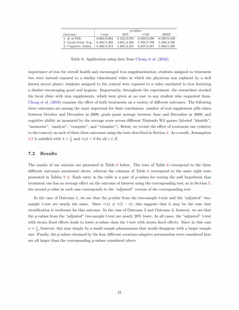
p-valuesOutcome t-test SFE CAP SFEP

1: # of Pills 0.063/0.062 0.102/0.070 0.599/0.599 0.599/0.5992: Grade Point Avg. 6.494/5.304 4.991/4.206 5.788/5.788 5.190/4.7903: Cognitive Ability 6.466/5.273 5.305/4.355 6.387/6.387 5.389/5.389

Table 6: Application using data from Chong et al. (2016)

importance of iron for overall health and encouraged iron supplementation; students assigned to treatment

two were instead exposed to a similar educational video in which the physician was replaced by a well

known soccer player; students assigned to the control were exposed to a video unrelated to iron featuring

a dentist encouraging good oral hygiene. Importantly, throughout the experiment, the researchers stocked

the local clinic with iron supplements, which were given at no cost to any student who requested them.

Chong et al. (2016) examine the effect of both treatments on a variety of different outcomes. The following

three outcomes are among the most important for their conclusions: number of iron supplement pills taken

between October and December in 2009; grade point average between June and December in 2009; and

cognitive ability as measured by the average score across different Nintendo Wii games (labeled “identify”,

“memorize”, “analyze”, “compute”, and “visualize”). Below, we revisit the effect of treatment one (relative

to the control) on each of these three outcomes using the tests described in Section 4. As a result, Assumption

2.2 is satisfied with π = 12 and τ(s) = 0 for all s ∈ S.

7.2 Results

The results of our exercise are presented in Table 6 below. The rows of Table 6 correspond to the three

different outcomes mentioned above, whereas the columns of Table 6 correspond to the same eight tests

presented in Tables 3–4. Each entry in the table is a pair of p-values for testing the null hypothesis that

treatment one has no average effect on the outcome of interest using the corresponding test; as in Section 5,

the second p-value in each case corresponds to the “adjusted” version of the corresponding test.

In the case of Outcome 1, we see that the p-value from the two-sample t-test and the “adjusted” two-

sample t-test are nearly the same. Since τ(s) 6= π(1 − π), this suggests that it may be the case that

stratification is irrelevant for this outcome. In the case of Outcome 2 and Outcome 3, however, we see that

the p-values from the “adjusted” two-sample t-test are nearly 20% lower. In all cases, the “adjusted” t-test

with strata fixed effects leads to lower p-values than the t-test with strata fixed effects. Since in this case

π = 12 , however, this may simply be a small sample phenomenon that would disappear with a larger sample

size. Finally, the p-values obtained by the four different covariate-adaptive permutation tests considered here

are all larger than the corresponding p-values considered above.

21

Appendix A Proof of the main results

Throughout the Appendix we employ the following notation, not necessarily introduced in the text.

σ2X(s) For a random variable X, σ2

X(s) = Var[X|S = s]

σ2X For a random variable X, σ2

X = Var[X]

µa For a ∈ 0, 1, E[Yi(a)]

Yi(a) For a ∈ 0, 1, Yi(a)− E[Yi(a)|Si]

ma(Zi) For a ∈ 0, 1, E[Yi(a)|Zi]− µaς2Y (π) 1

πσ2Y (1) + 1

1−πσ2Y (0)

ς2Y

(π) 1πσ

2Y (1)

+ 11−πσ

2Y (0)

ς2A(π)∑s∈S p(s)τ(s)( 1

πE[m1(Zi)|Si = s] + 11−πE[m0(Zi)|Si = s])2

ς2H∑s∈S p(s)(E[m1(Zi)|Si = s]− E[m0(Zi)|Si = s])2

ς2π(1−2π)2π2(1−π)2

∑s∈S p(s)τ(s) (E[m1(Zi)|Si = s]− E[m0(Zi)|Si = s])

2

n(s) Number of individuals in stratum s ∈ S

na(s) For a ∈ 0, 1, number of individuals with Ai = a in stratum s ∈ S

Table 7: Useful notation

A.1 Proof of Theorem 4.1

We start the proof by showing that

√n(Yn,1 − Yn,0 − θ(Q)

) d→ N(0, ς2Y (π) + ς2H + ς2A(π)

). (A-46)

Consider the following derivation:

√n(Yn,1 − Yn,0 − θ(Q)) =

√n

(1

n1

n∑i=1

(Yi(1)− µ1)Ai −1

n0

n∑i=1

(Yi(0)− µ0)(1−Ai)

)

= R∗n,11√n

n∑i=1

((1− π − Dn

n

)(Yi(1)− µ1)Ai −

(π +

Dnn

)(Yi(0)− µ0)(1−Ai)

)= R∗n,1(R∗n,2 +R∗n,3) ,

where we used Dn =∑s∈S Dn(s), n1

n= Dn

n+ π, and the following definitions:

R∗n,1 ≡(Dnn

+ π

)−1(1− π − Dn

n

)−1

,

R∗n,2 ≡1

2√n

n∑i=1

((Yi(1)− µ1)(1− π)Ai − (Yi(0)− µ0)π(1−Ai)) ,

R∗n,3 ≡ −Dn√n

1

n

n∑i=1

((Yi(1)− µ1)Ai + (Yi(0)− µ0)(1−Ai)) .

22

By Assumption 2.2.(b), Dnn

P→ 0, which in turn implies that R∗n,1P→ (π(1 − π))−1. Lemma B.1 implies R∗n,2

d→π(1− π)N(0, ς2

Y(π) + ς2H + ς2A(π)). Lemma B.3 and Assumption 2.2.(b) imply R∗n,3

P→ 0. The desired conclusion thus

follows from the continuous mapping theorem.

We next prove that

√n

√σ2n,1

n1+σ2n,0

n0

P→ ςY (π) . (A-47)

This follows from showing thatnσ2n,1

n1

P→ 1πσ2Y (1) and

nσ2n,0

n0

P→ 11−πσ

2Y (0). We only show the first result; the proof of

the second one is analogous. Start by writing Yn,1 as follows:

Yn,1 ≡1

n1

n∑i=1

AiYi = µ1 +n

n1

1

n

n∑i=1

Ai(Yi(1)− µ1) . (A-48)

Then consider the following derivation:

nσ2n,1

n1=

n

n1

1

n1

n∑i=1

(Yi − Yn,1)2Ai

=n

n1

1

n1

n∑i=1

(µ1 − Yn,1 + Yi(1)− µ1)2Ai

=n

n1

(n

n1

1

n

n∑i=1

(Yi(1)− µ1)2Ai − (µ1 − Yn,1)2)

=

(n

n1

)2

R?n,4 −(n

n1

)3

R?2n,5 ,

where we used (A-48) and the following definitions:

R?n,4 ≡ 1

n

n∑i=1

(Yi(1)− µ1)2Ai ,

R?n,5 ≡ 1

n

n∑i=1

(Yi(1)− µ1)Ai .

Since nn1

= (Dnn

+π)−1 and Dnn

P→ 0 by Assumption 2.2.(b), it follows that nn1

P→ 1π

. The result follows from showing

that R?n,4P→ πσ2

Y (1) and R?n,5P→ 0. Since E[(Yi(1)− µ1)2] = σ2

Y (1) and E[(Yi(1)− µ1)] = 0, this follows immediately

from Lemma B.3. Finally, note that Assumption 2.1 implies that ς2Y (π) > 0.

To prove that ς2Y

(π)+ ς2H + ς2A(π) ≤ ς2Y (π) holds with strict inequality unless (12) holds, notice that for a ∈ 0, 1,

σ2Y (a) = σ2

Y (a) −∑s∈S

E[(Yi(1)− µ1)|Si = s]2p(s) = σ2Y (a) −

∑s∈S

E[ma(Zi)|Si = s]2p(s) . (A-49)

Using (A-49), we see that

ς2Y (π)− ς2Y (π)− ς2H − ς2A(π) =1

π(σ2Y (1) − σ2

Y (1)) +1

1− π (σ2Y (0) − σ2

Y (0))

−∑s∈S

p(s)(E[m1(Zi)|Si = s]− E[m0(Zi)|Si = s])2

−∑s∈S

p(s)τ(s)

(1

πE[m1(Zi)|Si = s] +

1

1− πE[m0(Zi)|Si = s]

)2

=∑s∈S

p(s) (π(1− π)− τ(s))

(1

πE[m1(Zi)|Si = s] +

1

1− πE[m0(Zi)|Si = s]

)2

,

23

where, by Assumption 2.2.(b), 0 ≤ τ(s) ≤ π(1− π). The right-hand side of this last display is non-negative and it is

zero if and only if (12) holds, as required.

A.2 Proof of Theorem 4.2

As noted in the text, the proof of Theorem 4.1 establishes that (15) holds. Note further that Assumption 2.1 implies

that ς2Y

(π) > 0. To complete the proof, we argue that ς2Y

(π), ς2H , and ς2A(π) defined in (20)–(22) satisfy ς2Y

(π)P→ ς2

Y(π),

ς2HP→ ς2H , and ς2A(π)

P→ ς2A(π).

We begin by noting some preliminary facts that will be useful in the analysis of these estimators. First, the weak

law of large numbers implies that n(s)n

= 1n

∑1≤i≤n ISi = s P→ p(s). Second, for a ∈ 0, 1, Yn,a

P→ µa. For the case

of Yn,1, this follows by writing Yn,1 as in (A-48), arguing as in the proof of Theorem 4.1 to establish that nn1

P→ 1π

,

and applying Lemma B.3. A similar argument establishes the result for Yn,0. Finally, for a ∈ 0, 1, µn,a(s) defined

in (19) converges in probability to E[Yi(a)|Si = s]. We prove this for the case of µn,1(s); an analogous argument

establishes it for µn,0(s). Begin by writing

µn,1(s) =1

n1(s)

∑1≤i≤n

YiIAi = 1, Si = s =n

n1(s)

1

n

∑1≤i≤n

Yi(1)ISi = sAi .

From Assumption 2.2.(b), n1(s)n

= Dn(s)n

+ π n(s)n

P→ πp(s). Lemma B.3 implies that

1

n

∑1≤i≤n

Yi(1)ISi = sAiP→ πE[Yi(1)ISi = s] .

The desired conclusion about µn,0(s) now follows immediately.

Now consider ς2Y

(π). For a ∈ 0, 1, note that

Var[Yi(a)] = E[(Yi(a)− E[Yi(a)|Si])2]

= E[Yi(a)2]− 2E[Yi(a)E[Yi(a)|Si]] + E[E[Yi(a)|Si]2]

= E[Yi(a)2]− E[E[Yi(a)|Si]2]

= E[Yi(a)2]−∑s∈S

p(s)E[Yi(a)|Si = s]2 .

Next, note that1

n1

∑1≤i≤n

Y 2i Ai =

n

n1

1

n

∑1≤i≤n

Yi(1)2Ai . (A-50)

By arguing as in the proof of Theorem 4.1 to establish that nn1

P→ 1π

and applying Lemma B.3, we see that (A-50)

converges in proability to E[Yi(1)2]. An analogous argument shows that

1

n0

∑1≤i≤n

Y 2i (1−Ai)

P→ E[Yi(0)2] .

Combining these convergences with the preliminary facts above, we see that ς2Y

(π)P→ ς2

Y(π).

Next, consider ς2H . For a ∈ 0, 1, note that

E[ma(Zi)|Si] = E[Yi(a)|Si]− µa . (A-51)

24

Hence,

ς2H =∑s∈S

p(s)((E[Yi(1)|Si = s]− µ1)− (E[Yi(0)|Si = s]− µ0))2 .

Using the preliminary facts above, we see that ς2HP→ ς2H .

Finally, consider ς2A(π). Using (A-51), we see that

ς2A(π) =∑s∈S

p(s)τ(s)

(1

π(E[Yi(1)|Si = s]− µ1)− 1

1− π (E[Yi(0)|Si = s]− µ0)

)2

.

Using the preliminary facts above, we again see that ς2A(π)P→ ς2A(π).

A.3 Proof of Theorem 4.3

We start the proof by showing that

√n(βn − θ(Q))

d→ N(0, ς2Y (π) + ς2H + ς2π) . (A-52)

To this end, write βn as

βn =

∑ni=1 AiYi∑ni=1 A

2i

,

where Ai is the projection of Ai on the strata indicators, i.e., Ai = Ai − n1(Si)/n(Si), where

n1(Si)

n(Si)=∑s∈S

ISi = sn1(s)

n(s).

Next, note that

√n(βn − θ(Q)) =

√n

1n

∑ni=1 A

2i

((1

n

n∑i=1

AiYi

)− θ(Q)

(1

n

n∑i=1

A2i

))

=1

1n

∑ni=1 A

2i

(√n

(1

n

n∑i=1

AiYi − π(1− π)θ(Q)

)− θ(Q)

√n

(1

n

n∑i=1

A2i − π(1− π)

)).

Below we argue that

√n

(1

n

n∑i=1

A2i − π(1− π)

)= (1− 2π)

∑s∈S

Dn(s)√n

+ oP (1) (A-53)

√n

(1

n

n∑i=1

AiYi − π(1− π)θ(Q)

)= Rn,1 +Rn,3 +Rn,4 + θ(Q)(1− 2π)

∑s∈S

Dn(s)√n

+ oP (1) , (A-54)

where Rn,1 and Rn,3 are defined as in (B-73) and (B-75) in Lemma B.1, and

Rn,4 ≡∑s∈S

Dn(s)√n

(1− 2π)(E[m1(Z)|S = s]− E[m0(Z)|S = s]) . (A-55)

25

Step 1: To see that (A-53) holds, let A∗i = Ai − π and note that

√n

(1

n

n∑i=1

A2i − π(1− π)

)=√n

(1

n

n∑i=1

AiAi − π(1− π)

)

=1√n

n∑i=1

(1− n1(Si)

n(Si)

)(Ai − π)− π√

n

n∑i=1

(n1(Si)

n(Si)− π

)

=∑s∈S

(1− n1(s)

n(s)

)1√n

n∑i=1

A∗i ISi = s − π√n

n∑i=1

(Dn(Si)

n(Si)

)

=∑s∈S

Dn(s)√n

(1− π)− π√n

∑s∈S

(Dn(s)

n(s)

) n∑i=1

ISi = s+ oP (1)

= (1− 2π)∑s∈S

Dn(s)√n

+ oP (1) , (A-56)

where the first equality follows from∑ni=1 Ai

n1(Si)n(Si)

= 0, the third equality follows from n1(s)n(s)

= Dn(s)n(s)

+ π, and the

fourth equality follows from n1(s)n(s)

P→ π for all s ∈ S, which in turn follows from the preliminary facts noted at the

beginning of the proof of Thoerem 4.2.

Step 2: To see that (A-54) holds, note that

√n

(1

n

n∑i=1

AiYi − π(1− π)θ(Q)

)=

1√n

n∑i=1

AiYi − π(1− π)√nθ(Q)− 1√

n

∑s∈S

n∑i=1

n1(s)

n(s)ISi = sYi . (A-57)

Consider the first two terms. Use that Ai = A∗i + π and the definition of Yi to get

1√n

n∑i=1

AiYi − π(1− π)√nθ(Q) =

1√n

n∑i=1

A∗i Yi +π√n

∑i=1

Yi − π(1− π)√nθ(Q)

=1√n

n∑i=1

[(Yi(1)− µ1)(1− π)Ai − (Yi(0)− µ0)π(1−Ai)] +π√n

∑i=1

Yi

+1√n

n∑i=1

[Ai(1− π)µ1 − (1−Ai)πµ0]−√nπ(1− π)(µ1 − µ0)

= Rn,1 +Rn,2 +Rn,3 +π√n

∑i=1

Yi +1√n

n∑i=1

A∗i [(1− π)µ1 + πµ0] , (A-58)

where the last equality follows from the proof of Lemma B.1. Now consider the third term in (A-57). Again using

26

the fact that n1(s)n(s)

= Dn(s)n(s)

+ π, we see that

1√n

∑s∈S

n∑i=1

n1(s)

n(s)ISi = sYi =

1√n

∑s∈S

n∑i=1

Dn(s)

n(s)ISi = sYi +

π√n

∑s∈S

n∑i=1

ISi = sYi

=∑s∈S

Dn(s)√n

n

n(s)

1

n

n∑i=1

ISi = sYi +π√n

n∑i=1

Yi

=∑s∈S

Dn(s)√n

n

n(s)p(s) (π(µ1 + E[m1(Z)|S = s]) + (1− π)(µ0 + E[m0(Z)|S = s]))

+π√n

n∑i=1

Yi + oP (1)

= Rn,2 +π√n

n∑i=1

Yi −∑s∈S

Dn(s)√n

(1− 2π)(E[m1(Z)|S = s]− E[m0(Z)|S = s])

+1√n

n∑i=1

A∗i (πµ1 + (1− π)µ0) + oP (1) . (A-59)

In the preceeding display, the third equality follows from

1

n

n∑i=1

ISi = sYi =1

n

n∑i=1

ISi = s(Yi(1)Ai + Yi(0)(1−Ai))

= πE[Yi(1)ISi = s] + (1− π)E[Yi(0)ISi = s]

= p(s) (π(µ1 + E[m1(Z)|S = s]) + (1− π)(µ0 + E[m0(Z)|S = s])) + oP (1) ,

which in turn follows from Lemma B.3, and the last equality follows from the fact that the weak law of large numbers

implies that nn(s)

= 1p(s)

+ oP (1), Assumption 2.2.(b) implies that Dn(s)√n

= OP (1) for all s ∈ S, and the definition of

Rn,2 in (B-74). Combining (A-57)–(A-59) and

1√n

n∑i=1

A∗i ((1− π)µ1 + πµ0)− 1√n

n∑i=1

A∗i (πµ1 + (1− π)µ0) = θ(Q)(1− 2π)∑s∈S

Dn(s)√n

,

we conclude that√n(βn − θ(Q)) =

1

π(1− π)(Rn,1 +Rn,3 +Rn,4) + oP (1) .

The result (A-52) now follows from the continuous mapping theorem and Lemma B.2.

Next, we prove that

Vn,β =

[(C′nCnn

)−1(C′n diagu2i : 1 ≤ i ≤ nCnn

)(C′nCnn

)−1][1,1]

P→ ς2Y (π) +

(1

π(1− π)− 3

)ς2H , (A-60)

where Cn is a n×|S|+1 matrix with the treatment assignment vector An in the first column and the strata indicators

vector in the rest of the columns, and ui is the least squares residual of the regression in (26). Note that 1nC′nCn

P→ ΣC,

where

ΣC ≡

π πp(1) πp(2) · · · πp(|S|)πp(1) p(1) 0 · · · 0

πp(2)...

. . ....

......

. . ....

πp(|S|) 0 · · · · · · p(|S|)

27

and

Σ−1C =

1π(1−π) − 1

1−π − 11−π · · · − 1

1−π

− 11−π

π1−π + 1

p(1)π

1−π · · · π1−π

− 11−π

π1−π

. . ....

......

. . ....

− 11−π

π1−π · · · · · · π

1−π + 1p(|S|)

. (A-61)

The convergence in probability follows from n1n

= Dnn

+ πP→ π, n1(s)

n= Dn(s)

n+ π n(s)

n

P→ πp(s), and n(s)n

P→ p(s) for

all s ∈ S. The second result follows from analytically computing the inverse matrix, which we omit here. It follows

that the [1, 1] component of Σ−1C equals (π(1− π))−1. Note further that

C′n diagu2i : 1 ≤ i ≤ nCnn

=1

n

∑ni=1 u

2iAi

∑ni=1 u

2iAiISi = 1 · · ·

∑ni=1 u

2iAiISi = |S|∑n

i=1 u2iAiISi = 1

∑ni=1 u

2i ISi = 1 · · · 0

......

. . ....∑n

i=1 u2iAiISi = |S| 0 · · ·

∑ni=1 u

2i ISi = |S|

.

It follows from Lemma B.9 thatC′n diagu2

i : 1 ≤ i ≤ nCnn

P→ Ω

where each component of the matrix Ω corresponds to the respective limits in Lemma B.9. It follows that

(C′nCnn

)−1(C′n diagu2i : 1 ≤ i ≤ nCnn

)(C′nCnn

)−1P→ Σ−1

C ΩΣ−1C =

ς2Y

(π) +(

1π(1−π) − 3

)ς2H V12

V′12 V22

,

where we omit the expressions of V12 and V22 as we do not need them for our arguments. From here, (A-60) follows

immediately. Finally, note that Assumption 2.1 implies that ς2Y

(π) > 0.

To prove that ς2Y

(π) + ς2H + ς2π ≤ ς2Y (π) +(

1π(1−π) − 3

)ς2H holds with strict inequality unless (30) holds, note that

(ς2Y (π) +

(1

π(1− π)− 3

)ς2H

)−(ς2Y (π) + ς2H + ς2π

)=

(1

π(1− π)− 4

)ς2H − ς2π

=∑s∈S

p(s)

((1

π(1− π)− 4

)− τ(s)

(1− 2π)2

π2(1− π)2

)(E[m1(Zi)|Si = s]− E[m0(Zi)|Si = s])2

= p(s)(1− 2π)2

π2(1− π)2(π(1− π)− τ(s))(E[m1(Zi)|Si = s]− E[m0(Zi)|Si = s])2 .

The right-hand side of this last display is non-negative and it is zero if and only if (30) holds, as required.

A.4 Proof of Theorem 4.4

As noted in the text, the proof of Theorem 4.3 establishes that (32) holds. Note further that Assumption 2.1 implies

that ς2Y

(π) > 0. The proof of Theorem 4.2 establishes that ς2Y

(π)P→ ς2

Y(π) and ς2H

P→ ς2H . To complete the proof, we

argue that ς2πP→ ς2π. To see this, note using (A-51) that

ς2π =(1− 2π)2

π2(1− π)2

∑s∈S

p(s)τ(s)((E[Yi(1)|Si = s]− µ1)− (E[Yi(0)|Si = s]− µ0))2 .

28

Using the preliminary facts noted at the beginning of the proof of Theorem 4.2, the desired result follows.

A.5 Proof of Theorem 4.5

Below we assume without loss of generality that θ0 = 0; the general case follows from the same arguments with Yi

replaced by Yi − θ0Ai.

Let Gn|S(n) and G′n|S(n) ∼ Unif(Gn(S(n))) with Gn, G′n, and X(n) independent conditional on S(n). Define

ς2cap =ς2Y

(1− π) + ς2Hς2Y (1− π)

. (A-62)

We first argue that for Q such that θ(Q) = 0,

(Tn(GnX(n)), Tn(G′nX

(n)))d→ (T, T ′) , (A-63)

where T and T ′ are independent with common c.d.f. Φ(t/ςcap).

Step 1: Following Chung and Romano (2013), we start the proof of (A-63) by coupling the data X(n) with auxiliary

“data” X(n) = (Vi, Ai, Zi) : 1 ≤ i ≤ n constructed according to the following algorithm. Set I = 1, . . . , n and

Kn = 0. For each s ∈ S, repeat the following two stages n(s) times:

1. Stage 1: Draw Cj ∈ 0, 1 such that PCj = 1 = π.

2. Stage 2: If there exists i ∈ I such that Ai = Cj and Si = s, set Vj = Yi and set I = I \ i; otherwise, draw a

new, independent observation from the distribution of Yi(Cj)|Si = s, set it equal to Vj and set Kn = Kn + 1.

Note that Kn constructed in this way is an upper bound on the number of elements in Vi : 1 ≤ i ≤ n that are not

identically equal to elements in Yi : 1 ≤ i ≤ n. Indeed, there exists g0 ∈ Gn(S(n)) such that

Kn ≥n∑i=1

IVg0(i) 6= Yi .

Step 2: We now prove that for Q such that θ(Q) = 0 and

TUn (X(n)) ≡√n

(1

n1

n∑i=1

YiAi −1

n0

n∑i=1

Yi(1−Ai)

), (A-64)

it follows that

(TUn (GnX(n)), TUn (G′nX

(n)))d→ (TU , TU′) , (A-65)

where TU and TU′ are independent with common distribution given by N(0, ς2Y

(1 − π) + ς2H) when τ(s) = 0 for all

s ∈ S. Arguing as in the proof of Lemma 5.1 in Chung and Romano (2013), (A-65) follows by verifying the following

two conditions:

(TUn (GnX(n)), TUn (G′nX

(n)))d→ (TU , TU′) (A-66)

TUn (Gng0X(n))− TUn (GnX

(n)) = oP (1) . (A-67)

Lemma B.4 establishes (A-66) and Lemma B.5 establishes (A-67).

29

Step 3: Note that we can write Tn(GnX(n)) as

Tn(GnX(n)) =

TUn (GnX(n))

TLn (GnX(n)),

where TLn (X(n)) =√TL,1n (X(n)) + TL,0n (X(n)) with

TL,1n (X(n)) =n

n1

1

n1

n∑i=1

(Yi − Yn,1)2Ai

TL,0n (X(n)) =n

n0

1

n0

n∑i=1

(Yi − Yn,0)2(1−Ai) .

It follows that

TL,1n (GnX(n)) =

1(n1n

)2(

1

n

n∑i=1

(Yi(1)Ai + Yi(0)(1−Ai))2AGn(i) −(1n

∑ni=1(Yi(1)Ai + Yi(0)(1−Ai))AGn(i)

)2n1n

)

Assumption 2.2.(b) implies that n1n

= Dnn

+ πP→ π. Lemma B.3 implies that

1

n

n∑i=1

(Yi(1)Ai + Yi(0)(1−Ai))2AGn(i) =1

n

n∑i=1

(Yi(1)2Ai + Yi(0)2(1−Ai))AGn(i)

P→ π2E[Yi(1)2] + π(1− π)E[Yi(0)2] (A-68)

1

n

n∑i=1

(Yi(1)Ai + Yi(0)(1−Ai))AGn(i)P→ π2E[Yi(1)] + π(1− π)E[Yi(0)] .

Using the fact that E[Yi(1)] = E[Yi(0)], it follows that

TL,1n (GnX(n))

P→ 1

π(πσ2

Y (1) + (1− π)σ2Y (0)) .

A similar argument shows that TL,0n (GnX(n))

P→ 11−π (πσ2

Y (1) + (1− π)σ2Y (0)). It thus follows that

TLn (GnX(n))

P→ ςY (1− π) . (A-69)

Finally, note that Assumption 2.1 implies that ς2Y (1 − π) > 0. Combining (A-65) and (A-69), we see that (A-63)

holds.

It now follows from Lemma B.7 that ccapn (1− α)P→ ςcapΦ−1(1− α). When τ(s) = 0 for all s ∈ S, it follows that

ς2A = 0 and so ς2cap = ς2t-test whenever π = 12

or σ2Y (1)

= σ2Y (0)

and σ2Y (1) = σ2

Y (0). Combining this last result with

Theorem 4.1, we see that limn→∞E[φcapn (X(n))] = α whenever θ(Q) = θ0, completing the proof of the theorem.

A.6 Proof of Theorem 4.6

The proof follows closely the proof of Theorem 4.5, we therefore omit some details. As in the proof of Theorem 4.5,

we assume without loss of generality that θ0 = 0; the general case then follows from the same arguments with Yi

replaced by Yi− θ0Ai. Let Gn and G′n be defined as in the proof of Theorem 4.5. We first argue that for Q such that

θ(Q) = 0,

(Tn(GnX(n)), Tn(G′nX

(n)))d→ (T, T ′) , (A-70)

30

where T and T ′ are independent with common c.d.f. Φ(t). Note that we can write Tn(GnX(n)) as

Tn(GnX(n)) =

TUn (GnX(n))

TLn (GnX(n)),

where TUn (X(n)) is defined as in (A-64) and

TLn (X(n)) =√ς2Y

(π) + ς2H .

Recall that ς2Y

(π) and ς2H are defined in (20) and (21). Note also that ςA(π) is not included in the definition of

TLn (X(n)) because it is assumed that τ(s) = 0 for all s ∈ S. The proof of Theorem 4.5 shows that (A-65) holds. We

now argue that

TLn (GnX(n))

P→√ς2Y

(1− π) + ς2H . (A-71)

To see this, first note the following consequences of Lemma B.3:

1

n1

∑1≤i≤n

Y 2i AGn(i)

P→ πE[Yi(1)2] + (1− π)E[Yi(0)2] (A-72)

1

n0

∑1≤i≤n

Y 2i (1−AGn(i))

P→ πE[Yi(1)2] + (1− π)E[Yi(0)2]

1

n1

∑1≤i≤n

YiAGn(i)P→ πE[Yi(1)] + (1− π)E[Yi(0)]

1

n0

∑1≤i≤n

Yi(1−AGn(i))P→ πE[Yi(1)] + (1− π)E[Yi(0)]

1

n1(s)

∑1≤i≤n

YiISi = sAGn(i)P→ πE[Yi(1)|Si = s] + (1− π)E[Yi(0)|Si = s]

1

n0(s)

∑1≤i≤n

YiISi = s(1−AGn(i))P→ πE[Yi(1)|Si = s] + (1− π)E[Yi(0)|Si = s] .

The convergence (A-72) follows from Assumption 2.2.(b), which implies that n1n

= Dnn

+ πP→ π, and (A-68),

established in the proof of Thoerem 4.5. The remaining convergences can be established in a similar fashion. Using

these convergences, some calculation shows that (A-71) holds. Note further that Assumption 2.1 implies that ς2Y

(1−π) > 0. Combining (A-65) and (A-71), we see that (A-70) holds. It thus follows from Lemma B.7 that ccapn (1−α)

P→Φ−1(1−α). Combining this last result with Theorem 4.2, we see that limn→∞E[φcap

n (X(n))] = α whenever θ(Q) = θ0,

completing the proof of the theorem.

Appendix B Auxiliary Results

Lemma B.1. Suppose Q satisfies Assumption 2.1 and the treatment assignment mechanism satisfies Assumption

2.2. Then,

1√n

n∑i=1

((Yi(1)− µ1)(1− π)Ai − (Yi(0)− µ0)π(1−Ai))d→ π(1− π)N(0, ς2Y (π) + ς2H + ς2A(π)) ,

where ς2Y

(π), ς2H , and ς2A(π) are defined in Table 7.

31

Proof. Let Yi(a) ≡ Yi(a)− E[Yi(a)|Si], ma(Zi) ≡ E[Yi(a)|Zi]− µa, and consider the following derivation:

1√n

n∑i=1

((Yi(1)− µ1)(1− π)Ai − (Yi(0)− µ0)π(1−Ai))

=1√n

n∑i=1

(Yi(1)(1− π)Ai − Yi(0)π(1−Ai)

)+

1√n

n∑i=1

(E[m1(Zi)|Si](1− π)Ai − E[m0(Zi)|Si]π(1−Ai))

= Rn,1 +1√n

n∑i=1

A∗i

(∑s∈S

(1− π)E[m1(Zi)|Si = s]ISi = s+∑s∈S

πE[m0(Zi)|Si = s]ISi = s

)

+π(1− π)√

n

n∑i=1

(∑s∈S

E[m1(Zi)|Si = s]ISi = s −∑s∈S

E[m0(Zi)|Si = s]ISi = s

)= Rn,1 +Rn,2 +Rn,3 ,

where we used A∗i = Ai − π and the following definitions:

Rn,1 ≡π(1− π)√

n

n∑i=1

(1

πYi(1)Ai −

1

1− π Yi(0)(1−Ai))

(B-73)

Rn,2 ≡ π(1− π)∑s∈S

Dn(s)√n

(1

πE[m1(Zi)|Si = s] +

1

1− πE[m0(Zi)|Si = s]

)(B-74)

Rn,3 ≡ π(1− π)∑s∈S

√n

(n(s)

n− p(s)

)(E[m1(Zi)|Si = s]− E[m0(Zi)|Si = s]) . (B-75)

The result now follows immediately from Lemma B.2 and the continuous mapping theorem.

Lemma B.2. Suppose Q satisfies Assumption 2.1 and the treatment assignment mechanism satisfies Assumption

2.2. Let Rn,1, Rn,2, Rn,3, and Rn,4 be defined as in (B-73), (B-74), (B-75), and (A-55), respectively. Then,

(Rn,1, Rn,2, Rn,3)d→ (ζR1 , ζR2 , ζR3) , (B-76)

where ζR1 , ζR2 , and ζR3 are independent and satisfy ζR1 ∼ π(1 − π)N(0, ς2Y

(π)), ζR2 ∼ π(1 − π)N(0, ς2A(π)), and

ζR3 ∼ π(1− π)N(0, ς2H). Furthermore,

(Rn,1, Rn,4, Rn,3)d→ (ζR1 , ζR4 , ζR3) , (B-77)

where ζR1 , ζR4 , and ζR3 are independent and satisfy ζR1 ∼ π(1 − π)N(0, ς2Y

(π)), ζR4 ∼ π(1 − π)N(0, ς2π, and

ζR3 ∼ π(1− π)N(0, ς2H).

Proof. We prove only (B-76); an analogous argument establishes (B-77). To this end, we first argue that

(Rn,1, Rn,2, Rn,3)d= (R∗n,1, Rn,2, Rn,3) + oP (1) (B-78)

for a random variable R∗n,1 that satisfies R∗n,1 ⊥⊥ (Rn,2, Rn,3) and R∗n,1d→ ζR1 . To this end, note that under the

assumption that W (n) is i.i.d. and Assumption 2.2(a), the distribution of Rn,1 is the same as the distribution of the

same quantity where units are ordered by strata and then ordered by Ai = 1 first and Ai = 0 second within strata.

In order to exploit this observation, it is useful to introduce some further notation. Define N(s) ≡∑ni=1 ISi < s

and F (s) ≡ PSi < s for all s ∈ S. Furthermore, independently for each s ∈ S and independently of (A(n), S(n)),

let (Y si (1), Y si (0)) : 1 ≤ i ≤ n be i.i.d. with marginal distribution equal to the distribution of (Yi(1), Yi(0))|Si = s.

32

With this notation, define

Rn,1 ≡ π(1− π)∑s∈S

1√n

n(N(s)n

+n1(s)n

)∑i=n

N(s)n

+1

1

πY si (1)− 1√

n

n(N(s)n

+n(s)n

)∑i=n

(N(s)n

+n1(s)n

)+1

1

1− π Ysi (0)

. (B-79)

By construction, Rn,1|S(n), A(n) d= Rn,1|S(n), A(n), and so Rn,1

d= Rn,1. Since Rn,2 and Rn,3 are functions of

S(n) and A(n), we have further that (Rn,1, Rn,2, Rn,3)d= (Rn,1, Rn,2, Rn,3). Next, define

R∗n,1 ≡ π(1− π)∑s∈S

1√n

bn(F (s)+πp(s))c∑i=bnF (s)c+1

1

πY si (1)− 1√

n

bn(F (s)+p(s))c∑i=bn(F (s)+πp(s))c+1

1

1− π Ysi (0)

. (B-80)

Since R∗n,1 is a function of (Y si (1), Y si (0)) : 1 ≤ i ≤ n, s ∈ S ⊥⊥ (S(n), A(n)), and (Rn,2, Rn,3) is a function of

(S(n), A(n)), we see that R∗n,1 ⊥⊥ (Rn,2, Rn,3).

To complete the proof of (B-78), we establish that R∗n,1d→ ζR1 and ∆n ≡ Rn,1 −R∗n,1

P→ 0. To this end, consider

an arbitrary s ∈ S and define the following partial sum process:

gn(u) ≡ 1√n

bnuc∑i=1

Y si (1) .

Under our assumptions, this converges weakly to a suitably scaled Brownian motion (see, e.g., Shorack and Wellner

(2009, Theorem 1, page 53) or Durrett (2010, Theorem 8.6.5, page 328)). Indeed, by elementary properties of

Brownian motion, we have that

1√n

bn(F (s)+πp(s))c∑i=bnF (s)c+1

1

πY si (1)

d→ N

(0,p(s)σ2

Y (1)(s)

π

),

where we have used that σ2Y s(1)

= σ2Y (1)

(s). Furthermore, since

(N(s)

n,n1(s)

n

)P→ (F (s), πp(s)) ,

it follows that

gn

(N(s) + n1(s)

n

)− gn

(N(s)

n

)− (gn (F (s) + πp(s))− gn(F (s)))

P→ 0 ,

where the convergence follows from elementary properties of Brownian motion and the continuous mapping theorem.

Repeating an analogous argument for Y si (0) and using the independence of (Y si (1), Y si (0)) : 1 ≤ i ≤ n, s ∈ S across

both i and s, we conclude that R∗n,1d→ ζR1 and ∆n ≡ Rn,1 −R∗n,1

P→ 0.

From Assumption 2.2.(b) and the continuous mapping theorem,

Rn,2|S(n) d→ ζR2 a.s. (B-81)

Also, the central limit theorem and continuous mapping theorem imply that

Rn,3d→ ζR3 . (B-82)

To complete the proof, we show that (Rn,1, Rn,2, Rn,3)d→ (ζR1 , ζR2 , ζR3) with ζR1 , ζR2 , ζR3 independent. From

33

(B-78), it suffices to show that (R∗n,1, Rn,2, Rn,3)d→ (ζR1 , ζR2 , ζR3), i.e.,

PR∗n,1 ≤ h1PRn,2 ≤ h2, Rn,2 ≤ h3 → PζR1 ≤ h1PζR2 ≤ h2PζR3 ≤ h3 , (B-83)

for any h = (h1, h2, h3) ∈ R3 s.t. PζR1 ≤ h1PζR2 ≤ h2PζR3 ≤ h3 is continuous.

As a first case, we assume that PζR1 ≤ ·, PζR2 ≤ ·, and PζR3 ≤ · are continuous at h1, h2, h3, respectively.

Then, R∗n,1d→ ζR1 implies PR∗n,1 ≤ h1 → PζR1 ≤ h1 and (B-83) follows from the following argument:

PRn,2 ≤ h2, Rn,2 ≤ h3 = E[PRn,2 ≤ h2, Rn,3 ≤ h3|S(n)]

= E[PRn,2 ≤ h2|S(n)IRn,3 ≤ h3]

= E[(PRn,2 ≤ h2|S(n) − PζR2≤ h2)IRn,3 ≤ h3]

+ E[PζR2≤ h2IRn,3 ≤ h3]

= E[(PRn,2 ≤ h2|S(n) − PζR2 ≤ h2)IRn,3 ≤ h3] + PζR2 ≤ h2PRn,3 ≤ h3

→ PζR2≤ h2PζR3

≤ h3 ,

where the convergence follows from the dominated convergence theorem, (B-81), and (B-82).

Finally, we now consider the case in which PζRj ≤ · is discontinuous at hj for some 1 ≤ j ≤ 3. Since ζRj is

normally distributed, this implies that ζRj must be degenerate and equal to zero and thus hj = 0. In turn, since

PζR1 ≤ ·PζR2 ≤ ·PζR3 ≤ · is continuous at (h1, h2, h3), then this implies that Πk 6=jPζRk ≤ hk = 0. Since

ζRk for k 6= j are also normally distributed, this implies for some k 6= j that ζRk is also degenerate and equal to zero

and hk < 0. Then, (B-83) follows from the following argument:

PRn,1 ≤ h1, Rn,2 ≤ h2, Rn,2 ≤ h3 ≤ PRn,k ≤ hk

→ 0

= PζR1 ≤ h1PζR2 ≤ h2PζR3 ≤ h3 ,

where the convergence follows from hk < 0 and the fact that Rn,kd→ ζRk with ζRk degenerate and equal to zero, and

the final equality uses that PζRk ≤ hk = 0.

Lemma B.3. Suppose Q satisfies Assumption 2.1 and the treatment assignment mechanism satisfies Assumption

2.2. Let Wi = f(Yi(1), Yi(0), Si) for some function f(·) satisfy E[|Wi|] <∞. Then

1

n

n∑i=1

WiAiP→ πE[Wi] . (B-84)

Furthermore,

1

n

n∑i=1

WiAGn(i)P→ πE[Wi] (B-85)

1

n

n∑i=1

WiAiAGn(i)P→ π2E[Wi] (B-86)

for Gn|S(n) ∼ Unif(Gn(S(n))) with Gn and X(n) independent conditional on S(n).

Proof. We first prove (B-84). By arguing as in the proof of Lemma B.1, note that

1

n

n∑i=1

WiAid=∑s∈S

1

n

n1(s)∑i=1

W si ,

34

where, independently for each s ∈ S and independently of (A(n), S(n)), W si : 1 ≤ i ≤ n are i.i.d. with marginal

distribution equal to the distribution of Wi|Si = s. In order to establish the desired result, it suffices to show that

1

n

n1(s)∑i=1

W siP→ πp(s)E[W s

i ] . (B-87)

From Assumption 2.2.(b), n1(s)n

= Dn(s)n

+ π n(s)n

P→ πp(s), so (B-87) follows from

1

n1(s)

n1(s)∑i=1

W siP→ E[W s

i ] . (B-88)

To establish (B-88), use the almost sure representation theorem to construct n1(s)n

such that n1(s)n

d= n1(s)

nand

n1(s)n→ πp(s) a.s. Using the independence of (A(n), S(n)) and W s

i : 1 ≤ i ≤ n, we see that for any ε > 0,

P

∣∣∣∣∣∣ 1

n1(s)

n1(s)∑i=1

W si − E[W s

i ]

∣∣∣∣∣∣ > ε

= P

∣∣∣∣∣∣∣

1

nn1(s)n

nn1(s)n∑

i=1

W si − E[W s

i ]

∣∣∣∣∣∣∣ > ε

= P

∣∣∣∣∣∣∣

1

n n1(s)n

nn1(s)n∑

i=1

W si − E[W s

i ]

∣∣∣∣∣∣∣ > ε

= E

P∣∣∣∣∣∣∣

1

n n1(s)n

nn1(s)n∑

i=1

W si − E[W s

i ]

∣∣∣∣∣∣∣ > ε∣∣∣ n1(s)

n

→ 0 ,

where the convergence follows from the dominated convergence theorem and

P

∣∣∣∣∣∣∣

1

n n1(s)n

nn1(s)n∑

i=1

W si − E[W s

i ]

∣∣∣∣∣∣∣ > ε∣∣∣ n1(s)

n

→ 0 a.s. . (B-89)

To see that the convergence (B-89) holds, note that the weak law of large numbers implies that

1

nk

nk∑i=1

W siP→ E[W s

i ] (B-90)

for any subsequence nk →∞ as k →∞. Since n n1(s)n→∞ a.s., (B-89) follows from the independence of n1(s)

nand

W si : 1 ≤ i ≤ n and (B-90).

The convergence (B-85) follows from an analogous argument after conditioning on Gn. The convergence (B-86)

follows in the same way using additionally the convergence (B-97) established in the proof of Lemma B.4.

Lemma B.4. Suppose Q satisfies Assumption 2.1 and the treatment assignment mechanism satisfies Assumption 2.2

with τ(s) = 0 for all s ∈ S. Let Gn, G′n, and X(n) be defined as in the proof of Theorem 4.5. For TUn (X(n)) defined

in (A-64), we have that (A-66) holds whenever Q additionally satisfies θ(Q) = 0.

Proof. Let g = Gn and g′ = G′n. Note that

TUn (gX(n)) =1

(Dn/n+ π)(1− π −Dn/n)

(1√n

n∑i=1

ViA∗g(i) −

Dn√n

1

n

n∑i=1

Vi

),

35

where A∗i = Ai−π. Since Assumption 2.2.(b) holds with τ(s) = 0 for all s ∈ S, Dn√n

P→ 0. From the weak law of large

numbers, we have further that

1

n

n∑i=1

ViP→ E[Vi] .

It thus follows that

TUn (gX(n)) =1

π(1− π)

1√n

n∑i=1

ViA∗g(i) + oP (1) .

Repeating the same argument for TUn (g′X(n)), we see that

(TUn (gX(n)), TUn (g′X(n))) =1

π(1− π)

(1√n

n∑i=1

ViA∗g(i),

1√n

n∑i=1

ViA∗g′(i)

)+ oP (1) .

Using the Cramer-Wold device, it suffices to show for real numbers a and b that

1√n

n∑i=1

Vi(aA∗g(i) + bA∗g′(i))

d→ π(1− π)N(0, (a2 + b2)(ς2Y (1− π) + ς2H)) . (B-91)

Note that the left-hand side of (B-91) equals

1√n

n∑i=1

(Vi − E[Vi|Si])(aA∗g(i) + bA∗g′(i)) +1√n

n∑i=1

E[Vi|Si](aA∗g(i) + bA∗g′(i)) . (B-92)

Becausen∑i=1

A∗g(i)ISi = s =

n∑i=1

A∗g′(i)ISi = s = Dn(s) ,

the second term in (B-92) equals

1√n

∑s∈S

n∑i=1

E[Vi|Si = s]ISi = s(aA∗g(i) + bA∗g′(i)) = (a+ b)∑s∈S

E[Vi|Si = s]Dn(s)√

n= oP (1) ,

where in the last equality we again use the fact that Dn(s)√n

P→ 0. To analyze the first term in (B-92), define

ns(d, d′) = |1 ≤ i ≤ n : Ag(i) ≤ d,Ag′(i) ≤ d′, Si = s| .

By arguing as in the proof of Lemma B.1, we see that this term is equal in distribution to the following:

∑s∈S

1√n

ns(0,0)∑i=1

V si (−π(a+ b)) +

ns(0,1)∑i=ns(0,0)+1

V si ((1− π)b− πa)

+

ns(1,0)∑i=ns(0,1)+1

V si ((1− π)a− πb) +

ns(1,1)∑i=ns(1,0)+1

V si (1− π)(a+ b)

, (B-93)

where, independently for each s ∈ S and independently of (A(n), S(n), g, g′), V si : 1 ≤ i ≤ n are i.i.d. with marginal

36

distribution equal to the distribution of Vi − E[Vi|Si]|Si = s. Next we argue that

ns(0, 0)

n

P→ (1− π)2p(s) (B-94)

ns(0, 1)− ns(0, 0)

n

P→ π(1− π)p(s) (B-95)

ns(1, 0)− ns(0, 1)

n

P→ π(1− π)p(s) (B-96)

ns(1, 1)− ns(1, 0)

n

P→ π2p(s) . (B-97)

We prove only (B-94); an analogous arugment establishes (B-95)–(B-97). Conditional on A(n) and S(n), ns(0, 0) is

a hypergeometric random variable corresponding to n0(s) draws from an urn with n(s) balls and n0(s) successes.

Hence,

E

[ns(0, 0)

n

∣∣A(n), S(n)

]=n0(s)2

n(s)n

P→ (1− π)2p(s) (B-98)

Var

[ns(0, 0)

n

∣∣A(n), S(n)

]=

n0(s)2n1(s)2

n2n(s)2(n(s)− 1)2P→ 0 ,

where the convergences in probability follow, as before, using Assumption 2.2.(b). It therefore follows by Chebychev’s

inequality (applied conditionally) that

P

∣∣∣∣ns(0, 0)

n− n0(s)2

n(s)n

∣∣∣∣ > ε∣∣A(n), S(n)

P→ 0 ,

which implies further thatns(0, 0)

n− n0(s)2

n(s)n

P→ 0 .

The convergence (B-94) thus follows from (B-98).

Therefore, again by arguing as in the proof of Lemma B.1, we see that (B-93) converges in distribution to a

normal with mean zero and variance given by

∑s∈S

π2(1− π)2

2π(1− π)(a+ b)2 + ((1− π)b− πa)2 + ((1− π)a− πb)2 p(s) Var[Vi|Si = s]

π(1− π)

= π2(1− π)2(a2 + b2)∑s∈S

p(s)Var[Vi|Si = s]

π(1− π). (B-99)

To complete the proof, note that

Var[Vi|Si = s] = πVar[Yi(1)|Si = s] + (1− π)Var[Yi(0)|Si = s]

+(πE[Yi(1)|Si = s]2 + (1− π)E[Yi(0)|Si = s]2

)− (πE[Yi(1)|Si = s] + (1− π)E[Yi(0)|Si = s])2

= πσ2Y (1)(s) + (1− π)σ2

Y (0)(s) +1

4(E[Yi(1)|Si = s]− E[Yi(0)|Si = s])2

= πσ2Y (1)(s) + (1− π)σ2

Y (0)(s) + π(1− π)(E[m1(Zi)|Si = s]− E[m0(Zi)|Si = s])2 ,

where in the final equality we have used the fact that µ1 = µ0 because θ(Q) = 0. It thus follows from the expressions

for ς2Y

(π) and ς2H in Table 7 that (B-99) equals π2(1− π)2(a2 + b2)(ς2Y

(1− π) + ς2H), and (B-91) follows.

Lemma B.5. Suppose Q satisfies Assumption 2.1 and the treatment assignment mechanism satisfies Assumption

2.2. Let Gn, g0 and X(n) be defined as in the proof of Theorem 4.5. Let TUn (X(n)) be defined as in (A-64). Then

37

(A-67) holds whenever Q additionally satisfies θ(Q) = 0.

Proof. Let g = Gn. Note that (A-67) equals

√n

(1

n1

n∑i=1

(Vgg0(i) − Yg(i))Ai −1

n0

n∑i=1

(Vgg0(i) − Yg(i))(1−Ai)

). (B-100)

Since

Yg(i) = Yg(i)(1)Ag(i) + Yg(i)(0)(1−Ag(i)) ,

we have that (B-100) equals

√n

(1

n1

n∑i=1

(Vgg0(i) − Yg(i)(1))Ag(i)Ai +1

n1

n∑i=1

(Vgg0(i) − Yg(i)(0))(1−Ag(i))Ai

− 1

n0

n∑i=1

(Vgg0(i) − Yg(i)(1))Ag(i)(1−Ai)−1

n0

n∑i=1

(Vgg0(i) − Yg(i)(0))(1−Ag(i))(1−Ai)

). (B-101)

By construction, all but at most Kn of the terms in the four summations in (B-101) must be identically equal to

zero. Moreover, conditionally on g, g0, A(n) and Kn, (B-101) has mean equal to zero. This follows from the fact that

E[Vi] = πµ1 + (1 − π)µ0 and µ1 − µ0 = 0 because θ(Q) = 0. Using the fact that Var[A + B] ≤ 2(Var[A] + Var[B]),

we see that, conditionally on g, g0, A(n) and Kn, (B-101) has variance bounded above by

Kn

n

((n

n1

)2

+

(n

n0

)2)M ,

where

M = 4 maxVar[Vi − Yi(1)],Var[Vi − Yi(0)] . (B-102)

Lemma B.6 implies that Knn

P→ 0. It therefore follows by Chebychev’s inequality (applied conditionally) that

P|TUn (gg0Xn)− TUn (gX(n))| > ε|g, g0, A(n),KnP→ 0 ,

from which the desired unconditional convergence (A-67) also follows.

Lemma B.6. Suppose Q satisfies Assumption 2.1 and the treatment assignment mechanism satisfies Assumption

2.2. Let Kn be defined as in the proof of Theorem 4.5. Then,

Kn

n

P→ 0 . (B-103)

Proof. The argument provided here follows closely arguments in Chung and Romano (2013). For each s, let Na(s) =

|Cj = a : j = 1, . . . , n(s)| for Cj as in the proof of Theorem 4.5. In this notation,

Kn =∑s∈S

∑a∈0,1

maxna(s)−Na(s), 0 .

In order to show (B-103), it suffices to show that for all s ∈ S and a ∈ 0, 1,

na(s)−Na(s)

n

P→ 0 . (B-104)

38

We prove (B-104) for the case a = 1; an analogous argument establishes it for the case a = 0. To this end, write

n1(s)−N1(s)

n=

(n1(s)

n− πn(s)

n

)−(N1(s)

n− πn(s)

n

)=

Dn(s)

n− n(s)

n

(N1(s)

n(s)− π

).

Under our assumptions, Dn(s)n

P→ 0 and n(s)n

P→ p(s). Note that for each s ∈ S, N1(s)|n(s) is distributed according to

a binomial distribution with n(s) trials and probability of success equal to π. It therefore follows from Chebychev’s

inequality (applied conditionally) that

P

∣∣∣∣N1(s)

n(s)− π

∣∣∣∣ > ε∣∣S(n)

≤ 1

nn(s)nε2

P→ 0 .

Hence,N1(s)

n(s)− π P→ 0 .

The desired result now follows.

Lemma B.7. Let Gn|S(n) and G′n|S(n) ∼ Unif(Gn(S(n))) with Gn, G′n, and X(n) independent conditional on S(n).

Suppose

(Tn(GnX(n)), Tn(G′nX

(n)))d→ (T, T ′) , (B-105)

where T ∼ T ′ with c.d.f. R(t) and T and T ′ are independent. Then, for any continuity point t of R,

Rn(t) =1

|Gn(S(n))|∑

g∈Gn(S(n))

ITn(gX(n)) ≤ t P→ R(t) .

Proof. Let t be a continuity point of R. Note that

E[Rn(t)] = E[E[Rn(t)|S(n)]]

= E

1

|Gn(S(n))|∑

g∈Gn(S(n))

PTn(gX(n)) ≤ t|S(n)

= E[PTn(GnX

(n)) ≤ t|S(n)]

= PTn(GnX(n)) ≤ t

→ R(t) ,

where the third equality follows from the distribution for Gn|S(n) and the independence of Gn and X(n) conditional

on S(n) and the convergence follows from (B-105). It therefore suffices to show that Var[Rn(t)]→ 0. Equivalently, it

is enough to show that E[R2n(t)]→ R2(t). To this end, note that

E[R2n(t)] = E

1

|Gn(S(n))|2∑

g∈Gn(S(n))

∑g′∈Gn(S(n))

ITn(gX(n)) ≤ t, Tn(g′X(n)) ≤ t

= E

1

|Gn(S(n))|2∑

g∈Gn(S(n))

∑g′∈Gn(S(n))

PTn(gX(n)) ≤ t, Tn(g′X(n)) ≤ t|S(n)

= E[PTn(GnX

(n)) ≤ t, Tn(G′nX(n)) ≤ t|S(n)]

= PTn(GnX(n)) ≤ t, Tn(G′nX

(n)) ≤ t

→ R2(t) ,

39

where, as before, the third equality follows from the distributions for Gn|S(n) and G′n|S(n) and the independence of

Gn, G′n, and X(n) conditional on S(n), and the convergence follows from (B-105).

Lemma B.8. Suppose Q satisfies Assumption 2.1 and the treatment assignment mechanism satisfies Assumption

2.2. Let γ = (β, δ1, . . . , δ|S|)′ be the parameters in the regression (26) and let γn be the least squares estimator of γ.

Then,

γnP→ γ ≡

θ(Q)

µ0 + πE[m1(Zi)|Si = 1] + (1− π)E[m0(Zi)|Si = 1]

...

µ0 + πE[m1(Zi)|Si = |S|] + (1− π)E[m0(Zi)|Si = |S|]

.

Proof. First note that γn = (C′nCn)−1C′nYn, where Cn is an n × (|S| + 1) matrix with the treatment assignment

vector An in the first row and the strata indicators vector in the rest of the rows, and Yn is an n × 1 vector of

outcomes. The (s+ 1)th element of 1nC′nYn equals 1

n

∑ni=1AiYi if s = 0 and 1

n

∑ni=1 ISi = sYi for s ∈ S. In turn,

this last term satisfies

1

n

n∑i=1

ISi = sYi =n1(s)

n(µ1 + E[m1(Zi)|Si = s]) +

(n(s)

n− n1(s)

n

)(µ0 + E[m0(Zi)|Si = s])

+1

n

n∑i=1

AiISi = sYi(1) +1

n

n∑i=1

(1−Ai) ISi = sYi(0)

= p(s) (π(µ1 + E[m1(Zi)|Si = s]) + (1− π)(µ0 + E[m0(Zi)|Si = s])) + oP (1) ,

where in the last step we used n1(s)n

= Dn(s)n

+ π n(s)n

P→ πp(s), n(s)n

P→ p(s), and that 1n

∑ni=1AiISi = sYi(a)

P→ 0

for a ∈ 0, 1 by Lemma B.3. Also by Lemma B.3,

1

n

n∑i=1

AiYi =1

n

n∑i=1

AiYi(1)P→ πµ1 ,

so that we conclude that

1

nC′nYn

P→

πµ1

p(1) (π(µ1 + E[m1(Zi)|Si = 1]) + (1− π)(µ0 + E[m0(Zi)|Si = 1]))

...

p(|S|) (π(µ1 + E[m1(Zi)|Si = 1]) + (1− π)(µ0 + E[m0(Zi)|Si = |S|]))

.

The result then follows from the above display, (A-61), and some additional algebra.

Lemma B.9. Suppose Q satisfies Assumption 2.1 and the treatment assignment mechanism satisfies Assumption

2.2. Let Ci ≡ [Ai, ISi = 1, . . . , ISi = |S|]′ be the ith row of the matrix Cn formed by stacking the treatment

assignment vector An in the first column and the strata indicators vector in the rest of the columns, ui be the

least squares residuals of the regression in (26), and γn be the least squares estimator of the regression coefficients

γ = (β, δ1, . . . , δ|S|)′. Then,

ui =∑s∈S

ISi = sA∗iE [m1(Zi)−m0(Zi)|Si = s] + Yi(1)Ai + Yi(0)(1−Ai) + Ci(γ − γn) . (B-106)

40

Furthermore,

1

n

n∑i=1

u2iP→ π(1− π)(ς2H + ς2Y (1− π)) (B-107)

1

n

n∑i=1

u2iAi

P→ π(1− π)2ς2H + πσ2Y (1) (B-108)

1

n

n∑i=1

u2i I Si = s P→ p(s)

(π(1− π) (E [m1(Zi)−m0(Zi)|Si = s])2 + πσ2

Y (1)(s) + (1− π)σ2Y (0)(s)

)(B-109)

1

n

n∑i=1

u2i I Si = sAi

P→ p(s)(π(1− π)2 (E [m1(Zi)−m0(Zi)|Si = s])2 + πσ2

Y (1)(s)). (B-110)

Proof. Consider the following derivation:

Yi = Yi(1)Ai + Yi(0)(1−Ai)

= θ(Q)Ai + µ0 + Yi(1)Ai + Yi(0)(1−Ai)

+∑s∈S

ISi = s (AiE[m1(Zi)|Si = s] + (1−Ai)E[m0(Zi)|Si = s]) .

Using Lemma B.8, we have that

Ciγ = θ(Q)Ai + µ0 +∑s∈S

ISi = s (πE[m1(Zi)|Si = s] + (1− π)E[m0(Zi)|Si = s]) .

Hence,

ui = Yi − Ciγ

=∑s∈S

ISi = sA∗iE [m1(Zi)−m0(Zi)|Si = s] + Yi(1)Ai + Yi(0) (1−Ai) . (B-111)

Since ui = ui + Ci(γ − γn), the desired expression for (B-106) follows.

To prove (B-107)–(B-110), note that for any univariate random variable Xi such that

1

n

n∑i=1

(C′iCi ⊗Xi

)= OP (1) and

1

n

n∑i=1

CiuiXi = OP (1) , (B-112)

we have that

1

n

n∑i=1

u2iXi =

1

n

n∑i=1

u2iXi + (γ − γn)′

1

n

n∑i=1

(C′iCi ⊗Xi

)(γ − γn) + 2(γ − γn)

1

n

n∑i=1

CiuiXi

=1

n

n∑i=1

u2iXi + oP (1) ,

where in the second equality we used γnP→ γ from Lemma B.8. Since the condition in (B-112) certainly holds for

Xi = 1, ISi = s, Ai, and ISi = sAi, it is enough to show that (B-107)–(B-110) holds with u2i in place of u2

i .

41

Using (B-111), we have that

u2i =

∑s∈S

(A∗i )2ISi = s (E [m1(Zi)−m0(Zi)|Si = s])2 + Yi(1)2Ai + Yi(0)2 (1−Ai)

+ 2∑s∈S

A∗i ISi = sE [m1(Zi)−m0(Zi)|Si = s] Yi(1)Ai

+ 2∑s∈S

A∗i ISi = sE [m1(Zi)−m0(Zi)|Si = s] Yi(0)(1−Ai) .

Lemma B.3 thus implies that

1

n

n∑i=1

u2iP→ π(1− π)

∑s∈S

p(s) (E [m1(Zi)−m0(Zi)|Si = s])2 + πσ2Y (1) + (1− π)

1

2σ2Y (0)

= π(1− π)(ς2H + ς2Y (1− π))

1

n

n∑i=1

u2iAi

P→ π(1− π)2∑s∈S

p(s) (E [m1(Zi)−m0(Zi)|Si = s])2 + πσ2Y (1)

= π(1− π)2ς2H + πσ2Y (1)

1

n

n∑i=1

u2i ISi = s P→ π(1− π)p(s)

((E [m1(Zi)−m0(Zi)|Si = s])2 +

1

1− πσ2Y (1)(s) +

1

πσ2Y (0)(s)

)1

n

n∑i=1

u2i ISi = sAi

P→ p(s)(π(1− π)2 (E [m1(Zi)−m0(Zi)|Si = s])2 + πσ2

Y (1)(s)),

thus completing the proof.

Lemma B.10. Suppose Q satisfies Assumption 2.1 and the treatment assignment mechanism satisfies Assumption

2.2. Then,

V homon,β =

(1

n

n∑i=1

u2i

)(C′nCnn

)−1

[1,1]

P→ ς2Y (1− π) + ς2H , (B-113)

where Cn and un are defined as in the proof of Theorem 4.3.

Proof. By arguing as in the proof of Theorem 4.3, we see that(C′nCnn

)−1

[1,1]

P→ [π(1− π)]−1 .

Lemma B.9 shows that 1n

∑ni=1 u

2iP→ π(1− π)

(ς2Y

(1− π) + ς2H). The desired result thus follows.

Lemma B.11. Let A(n) be a treatment assignment generated by the biased coin design mechanism described in

Example 3.2. Then, Assumption 2.2 holds.

Proof. Part (a) holds by definition. For part (b), note that for s 6= s′, Dn(s) ⊥⊥ Dn(s′)|S(n). Moreover, within

stratum the assignment is exactly the one considered in Markaryan and Rosenberger (2010, Theorem 2.1). It follows

from that result that

Dn(s)|S(n) = OP (1) a.s.

These two properties imply that part (b) holds with τ(s) = 0 for all s ∈ S.

Lemma B.12. Let A(n) be a treatment assignment generated by the adaptive biased coin design mechanism described

in Example 3.3. Then, Assumption 2.2 holds.

42

Proof. Part (a) holds by definition. Part (b) holds by Wei (1978, Theorem 3) adapted to account for stratification.

This result implies that Dn(s)√

n|S(n)

d→ N

(0,

1

4(1− 4ϕ′(0))

)a.s. (B-114)

Since Dn(s) ⊥⊥ Dn(s′)|S(n) for s 6= s′, part (b) holds with τ(s) = 14(1−4ϕ′(0)) for all s ∈ S.

Lemma B.13. Let A(n) be a treatment assignment generated by the stratified block randomization mechanism de-

scribed in Example 3.4. Then, Assumption 2.2 holds.

Proof. Part (a) follows by definition. Next note that, conditional on S(n), n(s) =∑ni=1 ISi = s and n1(s) = bn(s)

2c

are non-random. Thus, conditional on S(n), Dn(s) : s ∈ S is non-random with

Dn(s) =

0 if n(s) is even or n(s) = 0

−1 if n(s) is odd

for all s ∈ S. Part (b) then follows with τ(s) = 0 for all s ∈ S.

43

References

Berry, J., Karlan, D. S. and Pradhan, M. (2015). The impact of financial education for youth in

Ghana. Working paper.

Bruhn, M. and McKenzie, D. (2008). In pursuit of balance: Randomization in practice in development

field experiments. World Bank Policy Research Working Paper, 4752.

Bugni, F. A., Canay, I. A. and Shaikh, A. M. (2016). Inference under covariate adaptive randomization

with multiple treatments. In progress.

Callen, M., Gulzar, S., Hasanain, A., Khan, Y. and Rezaee, A. (2015). Personalities and public

sector performance: Evidence from a health experiment in Pakistan. Tech. rep., Working paper.

Chong, A., Cohen, I., Field, E., Nakasone, E. and Torero, M. (2016). Iron deficiency and schooling

attainment in peru. American Economic Journal: Applied Economics, 8 222–255.

Chung, E. and Romano, J. P. (2013). Exact and asymptotically robust permutation tests. The Annals

of Statistics, 41 484–507.

Dizon-Ross, R. (2014). Parents’ perceptions and children’s education: Experimental evidence from Malawi.

Manuscript, M.I.T.

Duflo, E., Dupas, P. and Kremer, M. (2014). Education, HIV, and early fertility: Experimental evidence

from kenya. Tech. rep., National Bureau of Economic Research.

Duflo, E., Glennerster, R. and Kremer, M. (2007). Using randomization in development economics

research: A toolkit. Handbook of development economics, 4 3895–3962.

Durrett, R. (2010). Probability: theory and examples. 4th ed. Cambridge university press.

Efron, B. (1971). Forcing a sequential experiment to be balanced. Biometrika, 58 403–417.

Heckman, J. J., Pinto, R., Shaikh, A. M. and Yavitz, A. (2011). Inference with imperfect randomiza-

tion: The case of the Perry Preschool. Manuscript.

Hoeffding, W. (1952). The large-sample power of tests based on permutations of observations. The Annals

of Mathematical Statistics, 23 pp. 169–192. URL http://www.jstor.org/stable/2236445.

Hu, Y. and Hu, F. (2012). Asymptotic properties of covariate-adaptive randomization. Annals of Statistics,

forthcoming.

Imbens, G. W. and Kolesar, M. (2012). Robust standard errors in small samples: some practical advice.

Tech. rep., National Bureau of Economic Research.

Imbens, G. W. and Rubin, D. B. (2015). Causal Inference for Statistics, Social, and Biomedical Sciences:

An Introduction. Cambridge University Press.

Kernan, W. N., Viscoli, C. M., Makuch, R. W., Brass, L. M. and Horwitz, R. I. (1999). Stratified

randomization for clinical trials. Journal of clinical epidemiology, 52 19–26.

44

Lee, S. and Shaikh, A. M. (2014). Multiple testing and heterogeneous treatment effects: Re-evaluating

the effect of progresa on school enrollment. Journal of Applied Econometrics, 29 612–626.

Lock Morgan, K. and Rubin, D. (2012). Rerandomization to improve covariate balance in experiments.

The Annals of Statistics, 40 1263–1282.

Markaryan, T. and Rosenberger, W. (2010). Exact properties of efron’s biased coin randomization

procedure. The Annals of Statistics, 38 1546–1567.

Pocock, S. and Simon, R. (1975). Sequential treatment assignment with balancing for prognostic factors

in the controlled clinical trial. Biometrics 103–115.

Rosenbaum, P. R. (2007). Interference between units in randomized experiments. Journal of the American

Statistical Association, 102.

Rosenberger, W. F. and Lachin, J. M. (2016). Randomization in clinical trials: theory and practice.

2nd ed. John Wiley & Sons.

Shao, J., Yu, X. and Zhong, B. (2010). A theory for testing hypotheses under covariate-adaptive ran-

domization. Biometrika, 97 347–360.

Shorack, G. R. and Wellner, J. A. (2009). Empirical processes with applications to statistics. Siam.

Wei, L. (1978). The adaptive biased coin design for sequential experiments. The Annals of Statistics, 6

92–100.

Young, A. (2016). Channeling fisher: Randomization tests and the statistical insignificance of seemingly

significant experimental results. Tech. rep., Technical Report, Working paper.

Zelen, M. (1974). The randomization and stratification of patients to clinical trials. Journal of chronic

diseases, 27 365–375.

45