INFERENCE ON K POPULATIONS.ANOVA

Jesús Piedrafita Arillajesus.piedrafita@uab.cat

Departament de Ciència Animal i dels Aliments

Curso de Formación de Personal Investigador Usuario de Animales para Experimentación

Learning objectives

Define the Completely Random Design, CRD (or One-way ANOVA).

Distinguish the between group variability from the within group variability.

Define a mathematical model describing CRD and distinguish the dependent and the independent variables.

Develop a procedure (ANOVA) to achieve an F test statistic: calculations with R Commander.

Explain the conditions of applicability of ANOVA (normality and within group homogeneous variances) and diagnostic procedures to test them.

Determine R2, the proportion in which the independent variable explains the dependent variable.

Define the idea of Multiple comparisons of means: Tukey test.

Power and sample size in ANOVA.

2

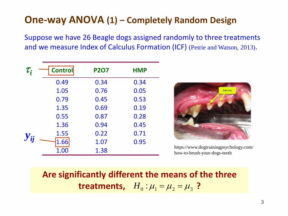
Are significantly different the means of the three treatments, ?

One-way ANOVA (1) – Completely Random Design

0 1 2 3:H

Suppose we have 26 Beagle dogs assigned randomly to three treatments and we measure Index of Calculus Formation (ICF) (Petrie and Watson, 2013).

Control P2O7 HMP

0.49 0.34 0.34 1.05 0.76 0.05 0.79 0.45 0.53 1.35 0.69 0.19 0.55 0.87 0.28 1.36 0.94 0.45 1.55 0.22 0.71 1.66 1.07 0.95 1.00 1.38

i

yij

3

https://www.dogtrainingpsychology.com/

how-to-brush-your-dogs-teeth

One-way ANOVA (2)

Between treatments variability

Within treatments variability

Total variability 4

Data: dogsICFGraphs > Strip chartFactors: Treatment; Response variable: ICF; Options: Stack

One-way ANOVA (3)

ijiijy

)()( ...... yyyyyy iiijij

Model:

Total SS, SST

where i) 1 t

j) 1 n, balanced design1 ni, unbalanced design

Between groups, SSB

Within groups (residual), SSW

Sums of squares (SS)

By squaring and summing these quantities, we arrive after some algebra at the computing formulas of the next slide

Level of a factor (fixed effect)

¡We make a partition of the variation!

Overall meanMean of level i

5

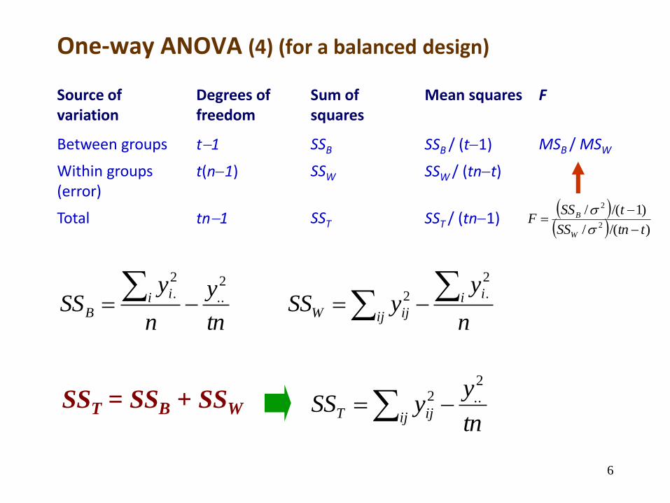
One-way ANOVA (4) (for a balanced design)

Source of variation

Degrees of freedom

Sum of squares

Mean squares F

Between groups t1 SSB SSB / (t1) MSB / MSW

Within groups (error)

t(n1) SSW SSW / (tnt)

Total tn1 SST SST / (tn1)

tn

y

n

ySS i i

B

2

..

2

.

n

yySS i i

ij ijW

2

.2

SST = SSB + SSWtn

yySS

ij ijT

2

..2

)/(/

)1/(/2

2

ttnSS

tSSF

W

B

6

One-way ANOVA (5), contrast of hypothesis

0

2

0

2

)(H

HMSE B

noti f

i f

2)( WMSE

0,1

)(

2

2

i ii i

Bt

nMSE

for

The null hypothesis and the alternative hypothesis can be stated as:

H0: 1 = 2 = 3 , the population means are equal

H1: i ≠ i’ , for at least one pair (i, i’), the means are not equal

An equivalent formulation of the hypothesis is:

H0: 1 = 2 = 3 , there is no difference among treatmentsH1: i ≠ i’ , for at least one pair (i, i’), a difference among treatments exist

It can be shown that the expectations of the mean squares are:

MSW is an unbiased estimator of σ2

02

2

2

11

)(

)(Ht

n

MSE

MSEF

i i

W

B noti f

7

One-way ANOVA (6), our example

Source of variation

Degrees of freedom

Sum of squares

Mean squares F

Between groups 3 1 = 2 17.2200 15.4154 = 1.8046

1.8046 / 2 = 0.9023 0.9023/ 0.1353 =

6.668

Within groups (error)

26 3 = 23 20.3320 17.2200 = 3.112

3.112 / 23 = 0.1353

2 2

.. (0.49 1.05 0.79 ... 0.45 0.71 0.95)15.4154

26

y

N

2 2 2 2

. 9.80 6.72 3.5017.22

9 9 8

i

ii

y

n

2 2 2 2 2 2 20.49 1.05 0.79 ... 0.45 0.71 0.95 20.332ijijy

> 1-pf(6.668,2,23)

[1] 0.005199879

Reject H0, p<0.05

8

p-value of F

This belongs to the era of calculators!!!

Conditions of applicability of ANOVA

9

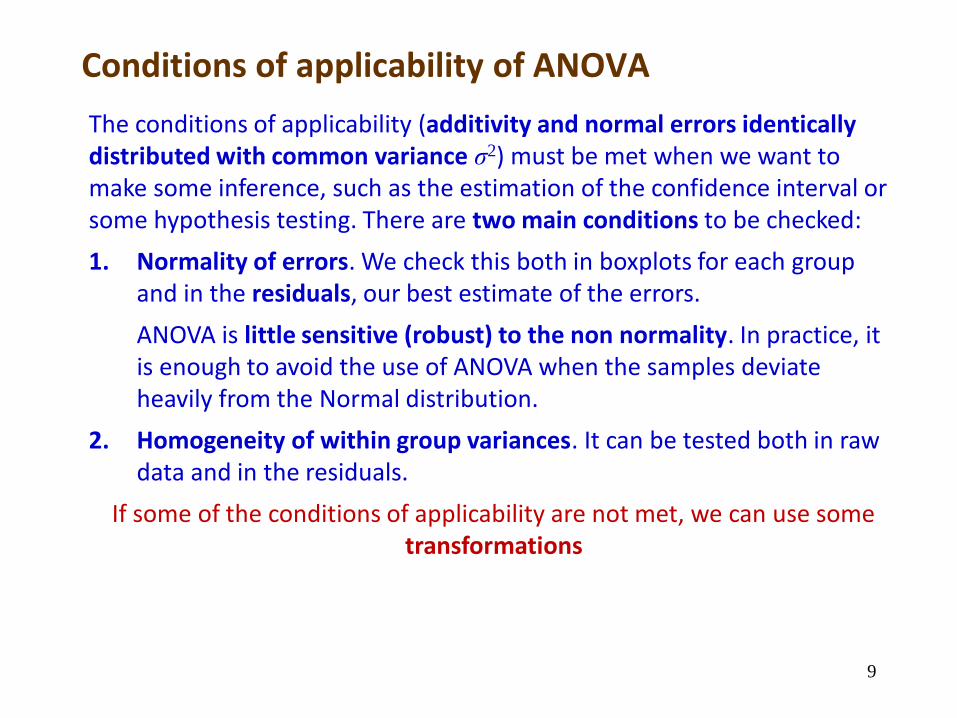
The conditions of applicability (additivity and normal errors identically distributed with common variance σ2) must be met when we want to make some inference, such as the estimation of the confidence interval or some hypothesis testing. There are two main conditions to be checked:

1. Normality of errors. We check this both in boxplots for each group and in the residuals, our best estimate of the errors.

ANOVA is little sensitive (robust) to the non normality. In practice, it is enough to avoid the use of ANOVA when the samples deviate heavily from the Normal distribution.

2. Homogeneity of within group variances. It can be tested both in raw data and in the residuals.

If some of the conditions of applicability are not met, we can use some transformations

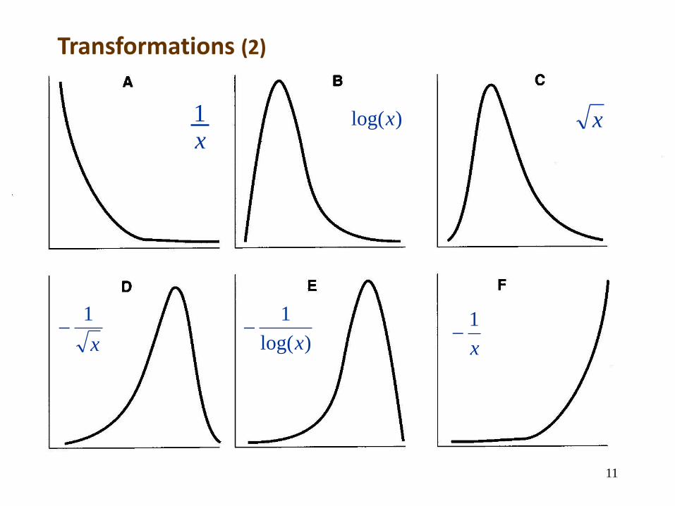
Transformations (1)

The objective is to normalise the distribution and/or to stabilise the variances. If transformations does not give satisfactory results, Non Parametric Tests can be used, such as Kruskal-Wallis test.

1. Logarithmic. When the treatments have a multiplicative effect, i.e., when they increment or decrement the measurements in a percent and not in a fixed quantity.

2. Root square. For data consisting of integers coming from counting (ticks on a cow). It tends to equalise 2.

3. Angular (arcsine). Data are the number of individuals with some

particular characteristic (percentages and proportions). Equalises 2.

4. Probit. For percentage data, like mortality. It is used in pharmacology.

5. Box-Cox. A general methodology to transform data.

To present a true mean value of data in the linear scale it is necessary to reconvert the

transformed mean. The standard deviation in this case is of no value and you should

compute confidence limits of the transformed data and then convert these to the linear scale.

10

x1 )log(x x

x

1

)log(

1

x

x

1

Transformations (2)

11

Working ANOVA – Boxplots (normality)

No obvious violations of normality and homogeneity of variance: boxplots not asymmetrical, do not vary greatly in size, no outliers

In addition to that we can suspect differences among groups when the boxes of some of the groups do not overlap

12

Graphs > BoxplotVariable: ICF; Plot by: Treatment

col=c("red", "green", "orange")

Levene's Test for Homogeneity of Variance

(center = "median")

Df F value Pr(>F)

group 2 0.7437 0.4864

23

Working ANOVA – Homogeneity of variances

Levene’s test confirms the homogeneity of variances of the three treatments (Pr(>F) = 0.4864)

This test is only needed if we suspect in the boxplot a clear heterogeneity of the within group variances

13

Statistics > VariancesFactors: Treatment; Response Variable: ICF

Working ANOVA – Anova table

The p-value of Treatment effect (p = 0.0052) allows us to reject the overall null hypothesis H0 of equality among the means of all treatments

Residual standard error (RSE) is an estimate of the within group standard deviation (“noise”). It is computed as the square root of the Residuals Mean Square:

RSE = 0.1353 = 0.367814

Statistics > Means> One-way AnovaGroups: Treatment; Response Variable: ICF✓Pairwise comparison of means

Df Sum Sq Mean Sq F value Pr(>F)

Treatment 2 1.805 0.9023 6.668 0.0052 **

Residuals 23 3.112 0.1353

---Signif. codes: 0 '***' 0.001 '**' 0.01 '*' 0.05 '.' 0.1 ' ' 1

Multiple comparisons

If H0 is not rejected, it is not necessary or appropriate to further analyse the problem, although the researcher must be aware of the possibility of a Type II error.

If H0 is rejected, then we must question which treatment or treatments caused a differential effect, that is, between which groups is the significant difference found.

For t treatments, there is a total of pair-wise comparisons of means. For each comparison there is the possibility of making Type I or Type II errors.

Looking at the experiment as a whole, the probability of making an error in conclusion is defined as the Experiment-wise Error Rate (EER).

There are many procedures of pair-wise comparisons of means: Bonferroni, Duncan, Dunnet, LSD, Scheffé, Student-Newman-Keuls, Tukey, among others.

2

t

15

Working ANOVA – Comparison of means, Tukey (1)

16

Treatment HMP differs significantly from Control, but P207 does not differ both from Control and HMP

Tukey’s Honestly Significant Difference

mean sd data:n

Control 1.0888889 0.4225353 9

HMP 0.4375000 0.2906520 8

P2O7 0.7466667 0.3695267 9

Multiple Comparisons of Means: Tukey Contrasts

Linear Hypotheses:

Estimate Std. Error t value Pr(>|t|)

HMP - Control == 0 -0.6514 0.1787 -3.644 0.00368 **

P2O7 - Control == 0 -0.3422 0.1734 -1.974 0.14128

P2O7 - HMP == 0 0.3092 0.1787 1.730 0.21572

Working ANOVA – Comparison of means, Tukey (2)

17

Observe how the two lower intervals in the figure contain 0, but in both extremes of the interval

Working ANOVA – Comparison of means, Tukey (3)

18

We can observe the numerical values used to construct the previous figure

The last two lines give us the grouping of means. HMP differs from Control, but not from P2O7. Control does not differ from P2O7.

Linear Hypotheses:

Estimate lwr upr

HMP - Control == 0 -0.65139 -1.09911 -0.20367

P2O7 - Control == 0 -0.34222 -0.77657 0.09213

P2O7 - HMP == 0 0.30917 -0.13855 0.75689

Control HMP P2O7

"b" "a" "ab"

Working ANOVA – Comparison of means, Dunnett

19

> library(DescTools)

> DunnettTest(ICF ~ Treatment, data = DogsICF)

Dunnett's test for comparing several treatments with a

control:

95% family-wise confidence level

$Control

diff lwr.ci upr.ci pval

HMP-Control -0.6513889 -1.0728610 -0.22991675 0.0026 **

P2O7-Control -0.3422222 -0.7511103 0.06666581 0.1081

In this test we have only contrasted the two treatments with the control. Only HMP presented a significant effect.

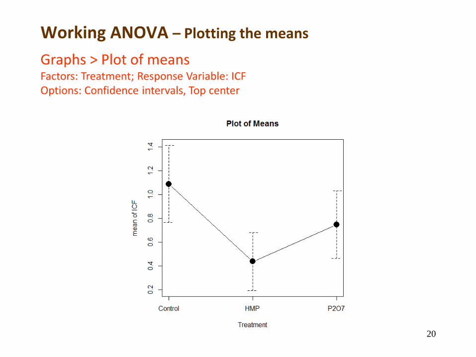
Working ANOVA – Plotting the means

20

Graphs > Plot of meansFactors: Treatment; Response Variable: ICFOptions: Confidence intervals, Top center

Working ANOVA – Analysis of residuals

No obvious violation of homogeneity of variance: residuals distributed randomly to both sides of the red line (0); no wedge shape in residuals

No obvious violation of normality: Q-Q plot of residuals is linear

iijij ye ˆˆˆ

21

Models > Graphs > Basic diagnostic plots

Working ANOVA – Power analysis

> MEANS <- tapply(dogsICF$ICF, dogsICF$Treatment, na.rm=T, mean)

> power.anova.test(groups=3, n=9, between.var=var(MEANS),

within.var=anova(AnovaModel.1)[[“Mean Sq"]][2], sig.level=0.05)

Balanced one-way analysis of variance power calculation

groups = 3

n = 9

between.var = 0.1061679

within.var = 0.135306

sig.level = 0.05

power = 0.8942738

NOTE: n is number in each group

22

We have a probability of almost 90% of rejecting H0 when false

The test has been developed for balanced ANOVA designs. In our case we assume 9 observations per group.

The students could resort to GRANMO: http://www.imim.cat/ofertadeserveis/granmo.html

> power.anova.test(groups=3, power=0.8, between.var=var(MEANS),

within.var=anova(AnovaModel.1)[[“Mean Sq"]][2], sig.level=0.05)

Balanced one-way analysis of variance power calculation

groups = 3

n = 7.237864

between.var = 0.1061679

within.var = 0.135306

sig.level = 0.05

power = 0.8

NOTE: n is number in each group

Working ANOVA – Sample size

23

We will have needed more than 7 animals (8) to detect as significant the differences observed between the means

As before, the students could resort also to GRANMO: http://www.imim.cat/ofertadeserveis/granmo.html