Inference for ProportionsInference for a Single Proportion

Chapter 8.1

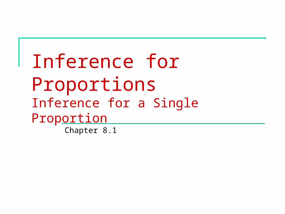
Sampling distribution of sample proportion The sampling distribution of a sample proportion is approximately

normal (normal approximation of a binomial distribution) when the

sample size is large enough.

p̂

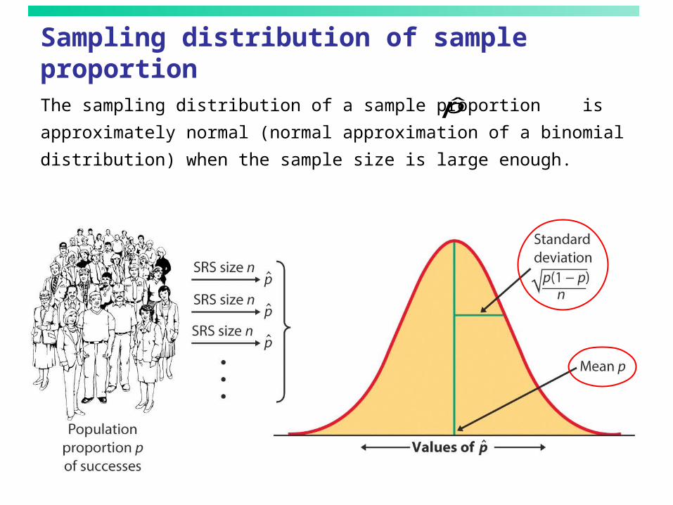
Conditions for inference on pAssumptions:

1. The data used for the estimate are an SRS from the population

studied.

2. The population is at least 10 times as large as the sample used for

inference. This ensures that the standard deviation of is close to

3. The sample size n is large enough that the sampling distribution

can be approximated with a normal distribution. How large a sample

size is required depends in part on the value of p and the test

conducted. Otherwise, rely on the binomial distribution.

p(1 p) n

p̂

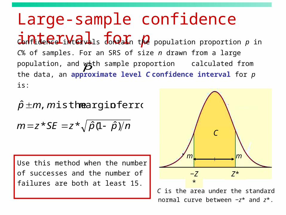
Large-sample confidence interval for p

Use this method when the number of

successes and the number of

failures are both at least 15.

C

Z*−Z*

m m

Confidence intervals contain the population proportion p in C% of

samples. For an SRS of size n drawn from a large population, and with

sample proportion calculated from the data, an approximate level C

confidence interval for p is:

C is the area under the standard

normal curve between −z* and z*.

nppzSEzm

mmp

)ˆ1(ˆ**

error ofmargin theis ,ˆ

p̂

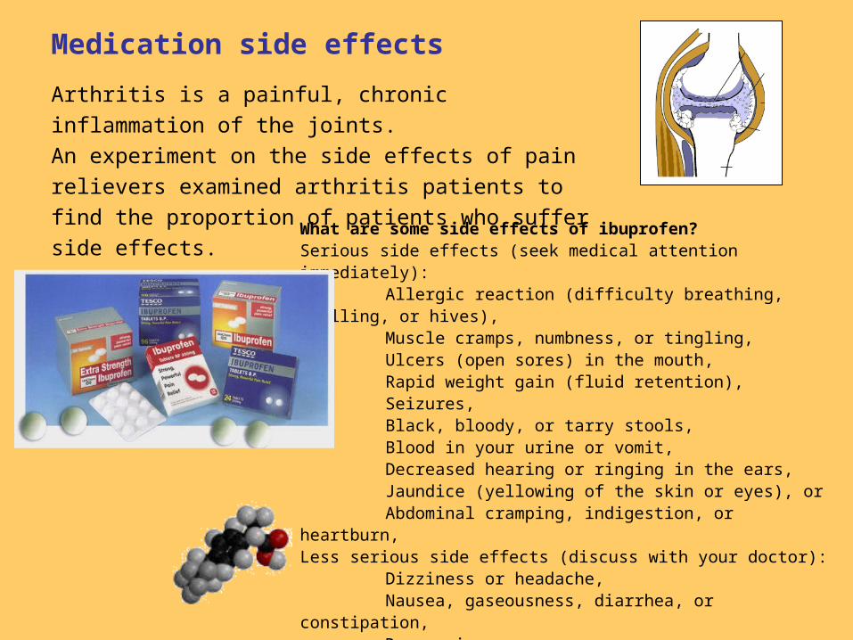
Medication side effects

Arthritis is a painful, chronic inflammation of the joints.

An experiment on the side effects of pain relievers

examined arthritis patients to find the proportion of

patients who suffer side effects.

What are some side effects of ibuprofen?Serious side effects (seek medical attention immediately):

Allergic reaction (difficulty breathing, swelling, or hives),Muscle cramps, numbness, or tingling,Ulcers (open sores) in the mouth,Rapid weight gain (fluid retention),Seizures,Black, bloody, or tarry stools,Blood in your urine or vomit,Decreased hearing or ringing in the ears,Jaundice (yellowing of the skin or eyes), orAbdominal cramping, indigestion, or heartburn,

Less serious side effects (discuss with your doctor):Dizziness or headache,Nausea, gaseousness, diarrhea, or constipation,Depression,Fatigue or weakness,Dry mouth, orIrregular menstrual periods

Upper tail probability P0.25 0.2 0.15 0.1 0.05 0.03 0.02 0.01

z* 0.67 0.841 1.036 1.282 1.645 1.960 2.054 2.32650% 60% 70% 80% 90% 95% 96% 98%

Confidence level C

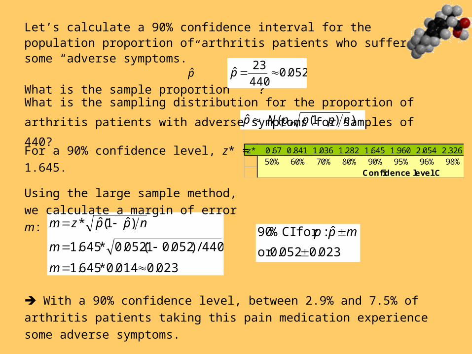
Let’s calculate a 90% confidence interval for the population proportion of arthritis patients who suffer some “adverse symptoms.”

What is the sample proportion ?

))1( ,( ˆ npppNp

023.0014.0*645.1

440/)052.01(052.0*645.1

)ˆ1(ˆ*

m

m

nppzm

052.0440

23ˆ p

What is the sampling distribution for the proportion of arthritis patients with

adverse symptoms for samples of 440?

For a 90% confidence level, z* = 1.645.

Using the large sample method, we

calculate a margin of error m:

With a 90% confidence level, between 2.9% and 7.5% of arthritis patients

taking this pain medication experience some adverse symptoms.

023.0052.0or

ˆ:forCI%90

mpp

p̂

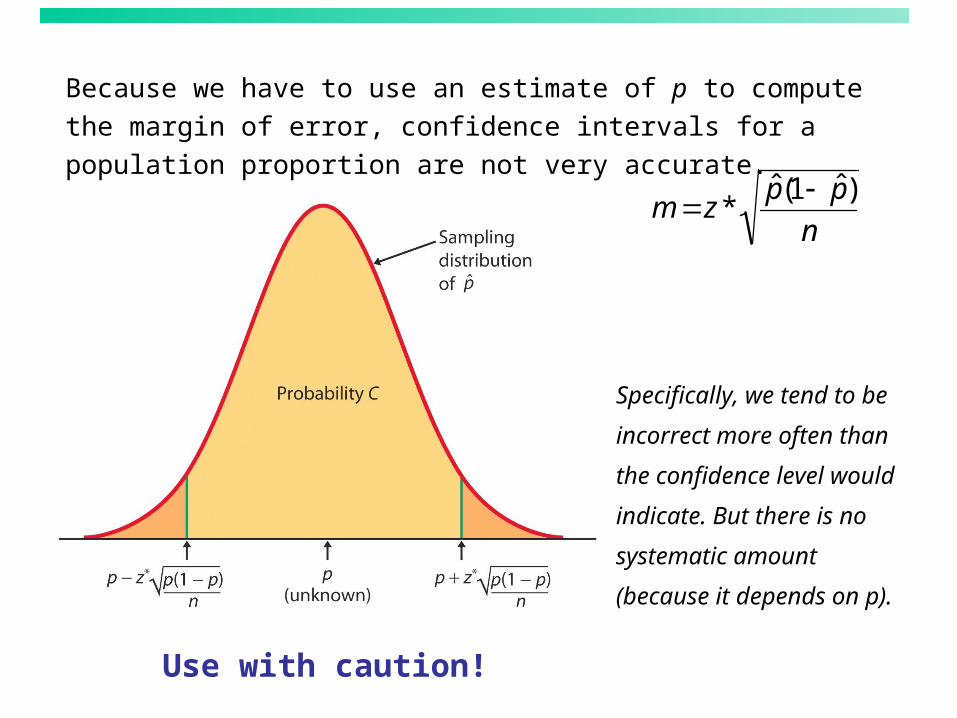
Because we have to use an estimate of p to compute the margin of

error, confidence intervals for a population proportion are not very

accurate.

m z *ˆ p (1 ˆ p )

n

Specifically, we tend to be

incorrect more often than

the confidence level would

indicate. But there is no

systematic amount

(because it depends on p).

Use with caution!

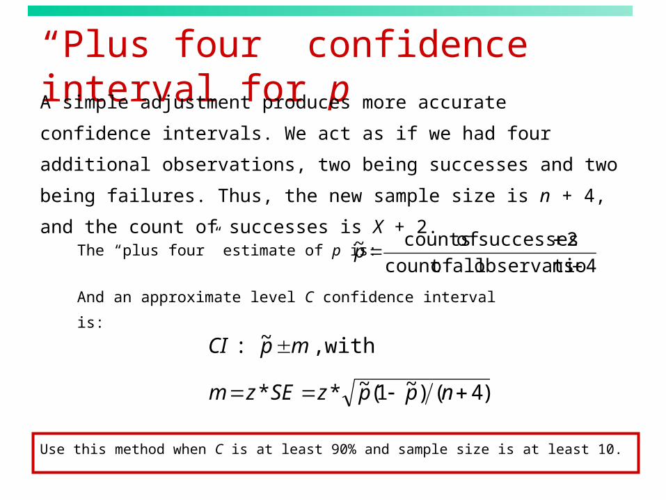
“Plus four” confidence interval for pA simple adjustment produces more accurate confidence intervals. We

act as if we had four additional observations, two being successes and

two being failures. Thus, the new sample size is n + 4, and the count of

successes is X + 2.

4nsobservatio all ofcount

2successes of counts~

p

)4()~1(~**

with,~:

nppzSEzm

mpCI

The “plus four” estimate of p is:

And an approximate level C confidence interval is:

Use this method when C is at least 90% and sample size is at least 10.

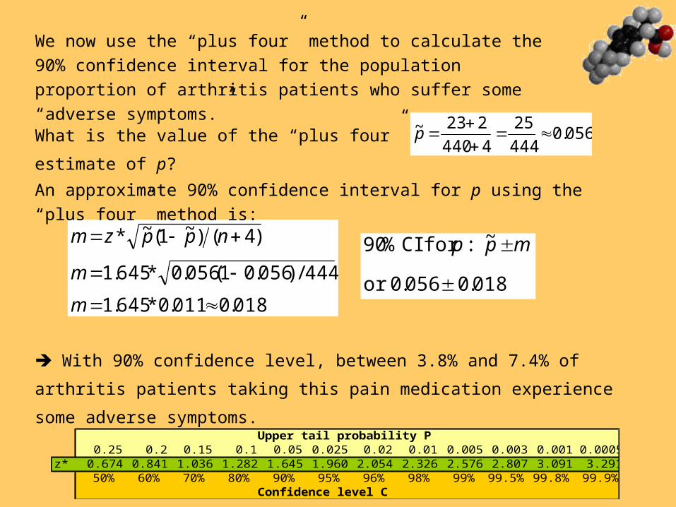
We now use the “plus four” method to calculate the 90% confidence

interval for the population proportion of arthritis patients who suffer

some “adverse symptoms.”

018.0011.0*645.1

444/)056.01(056.0*645.1

)4()~1(~*

m

m

nppzm

An approximate 90% confidence interval for p using the “plus four” method is:

Upper tail probability P0.25 0.2 0.15 0.1 0.05 0.025 0.02 0.01 0.005 0.003 0.001 0.0005

z* 0.674 0.841 1.036 1.282 1.645 1.960 2.054 2.326 2.576 2.807 3.091 3.29150% 60% 70% 80% 90% 95% 96% 98% 99% 99.5% 99.8% 99.9%

Confidence level C

With 90% confidence level, between 3.8% and 7.4% of arthritis patients

taking this pain medication experience some adverse symptoms.

018.0056.0or

~:forCI%90

mpp

056.0444

25

4440

223~

pWhat is the value of the “plus four” estimate of p?

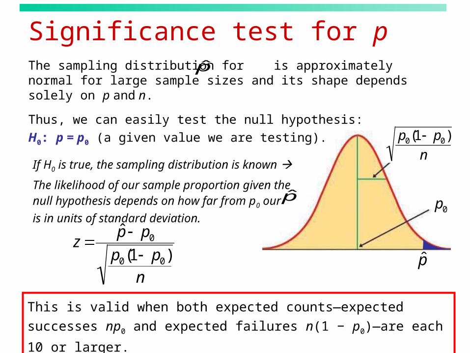
Significance test for pThe sampling distribution for is approximately normal for large sample sizes and its shape depends solely on p and n.

Thus, we can easily test the null hypothesis:

H0: p = p0 (a given value we are testing).

z ˆ p p0

p0(1 p0)

n

If H0 is true, the sampling distribution is known

The likelihood of our sample proportion given the null hypothesis depends on how far from p0 our

is in units of standard deviation.

This is valid when both expected counts—expected successes np0 and

expected failures n(1 − p0)—are each 10 or larger.

p0(1 p0)

n

p0

ˆ p

p̂

p̂

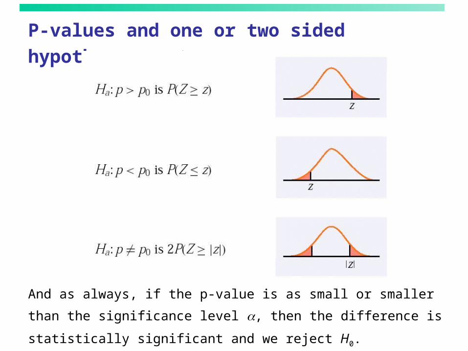
P-values and one or two sided hypotheses—reminder

And as always, if the p-value is as small or smaller than the significance

level , then the difference is statistically significant and we reject H0.

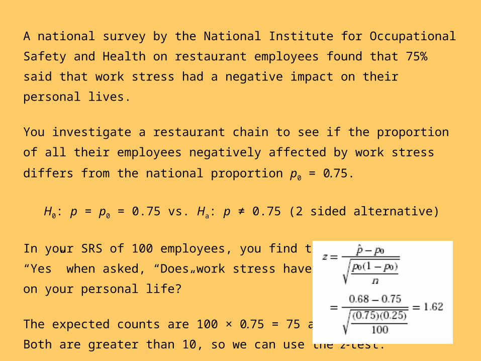
A national survey by the National Institute for Occupational Safety and Health on

restaurant employees found that 75% said that work stress had a negative impact

on their personal lives.

You investigate a restaurant chain to see if the proportion of all their employees

negatively affected by work stress differs from the national proportion p0 = 0.75.

H0: p = p0 = 0.75 vs. Ha: p ≠ 0.75 (2 sided alternative)

In your SRS of 100 employees, you find that 68 answered “Yes” when asked,

“Does work stress have a negative impact on your personal life?”

The expected counts are 100 × 0.75 = 75 and 25.

Both are greater than 10, so we can use the z-test.

The test statistic is:

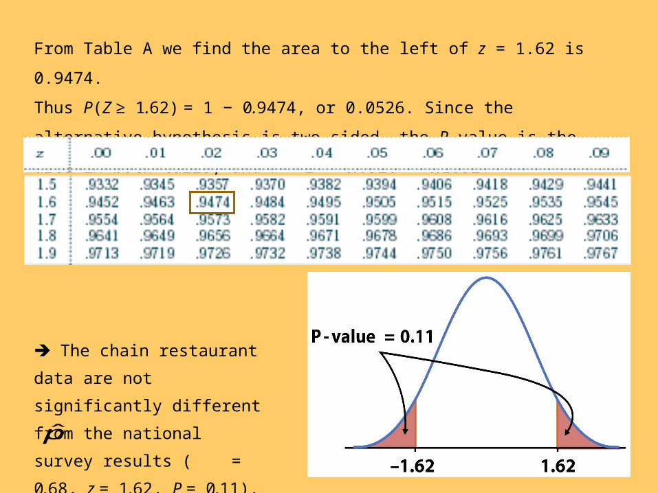
From Table A we find the area to the left of z = 1.62 is 0.9474.

Thus P(Z ≥ 1.62) = 1 − 0.9474, or 0.0526. Since the alternative hypothesis is

two-sided, the P-value is the area in both tails, and P = 2 × 0.0526 = 0.1052.

The chain restaurant data

are not significantly different

from the national survey results

( = 0.68, z = 1.62, P = 0.11).p̂

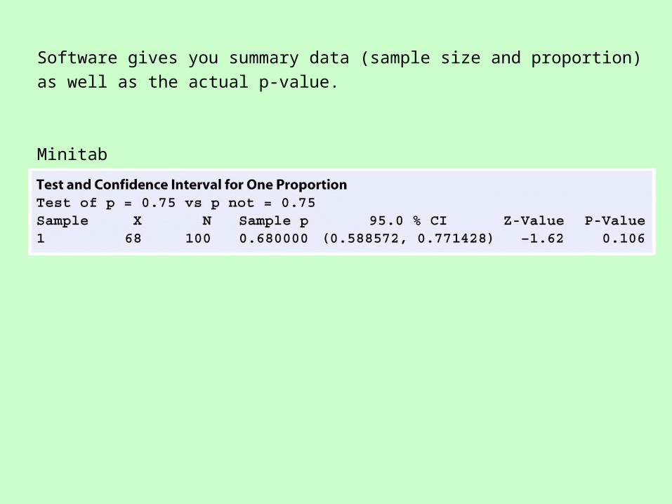
Software gives you summary data (sample size and proportion) as well as the

actual p-value.

Minitab

Interpretation: magnitude vs. reliability of effectsThe reliability of an interpretation is related to the strength of the

evidence. The smaller the p-value, the stronger the evidence against

the null hypothesis and the more confident you can be about your

interpretation.

The magnitude or size of an effect relates to the real-life relevance of

the phenomenon uncovered. The p-value does NOT assess the

relevance of the effect, nor its magnitude.

A confidence interval will assess the magnitude of the effect.

However, magnitude is not necessarily equivalent to how theoretically

or practically relevant an effect is.

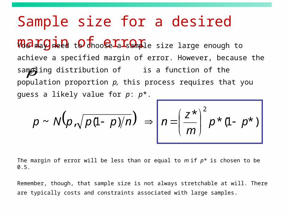
Sample size for a desired margin of errorYou may need to choose a sample size large enough to achieve a

specified margin of error. However, because the sampling distribution

of is a function of the population proportion p, this process requires

that you guess a likely value for p: p*.

The margin of error will be less than or equal to m if p* is chosen to be 0.5.

Remember, though, that sample size is not always stretchable at will. There are

typically costs and constraints associated with large samples.

*)1(**

)1(,~2

ppm

znnpppNp

p̂

Upper tail probability P0.25 0.2 0.15 0.1 0.05 0.03 0.02 0.01

z* 0.67 0.841 1.036 1.282 1.645 1.960 2.054 2.32650% 60% 70% 80% 90% 95% 96% 98%

Confidence level C

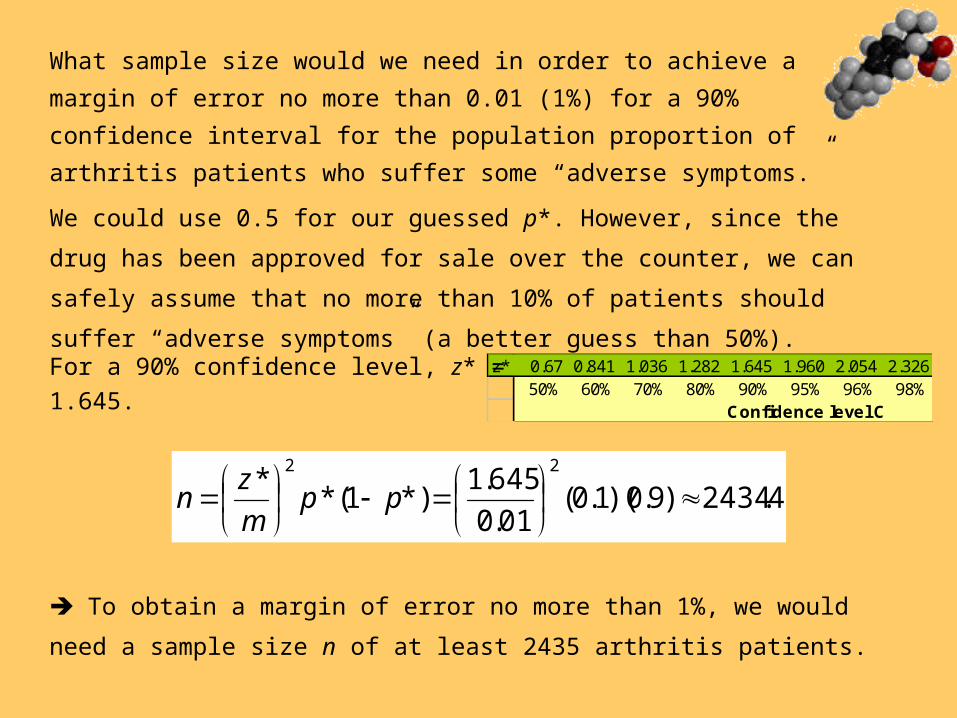
What sample size would we need in order to achieve a margin of error no

more than 0.01 (1%) for a 90% confidence interval for the population

proportion of arthritis patients who suffer some “adverse symptoms.”

4.2434)9.0)(1.0(01.0

645.1*)1(*

*22

pp

m

zn

We could use 0.5 for our guessed p*. However, since the drug has been

approved for sale over the counter, we can safely assume that no more than

10% of patients should suffer “adverse symptoms” (a better guess than 50%).

For a 90% confidence level, z* = 1.645.

To obtain a margin of error no more than 1%, we would need a sample

size n of at least 2435 arthritis patients.

Inference for ProportionsComparing Two Proportions

Chapter 8.2

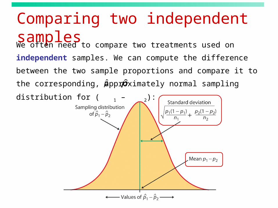
Comparing two independent samplesWe often need to compare two treatments used on independent

samples. We can compute the difference between the two sample

proportions and compare it to the corresponding, approximately normal

sampling distribution for ( 1 – 2):p̂ p̂

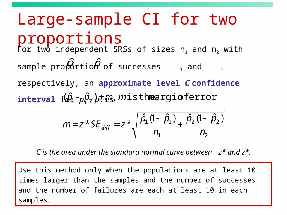
Large-sample CI for two proportionsFor two independent SRSs of sizes n1 and n2 with sample proportion

of successes 1 and 2 respectively, an approximate level C

confidence interval for p1 – p2 is

2

22

1

11

21

)ˆ1(ˆ)ˆ1(ˆ**

error ofmargin theis ,)ˆˆ(

n

pp

n

ppzSEzm

mmpp

diff

Use this method only when the populations are at least 10 times larger

than the samples and the number of successes and the number of

failures are each at least 10 in each samples.

C is the area under the standard normal curve between −z* and z*.

p̂ p̂

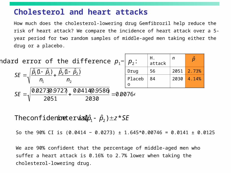
Cholesterol and heart attacks

How much does the cholesterol-lowering drug Gemfibrozil help reduce the risk

of heart attack? We compare the incidence of heart attack over a 5-year period

for two random samples of middle-aged men taking either the drug or a placebo.

So the 90% CI is (0.0414 − 0.0273) ± 1.645*0.00746 = 0.0141 ± 0.0125

We are 90% confident that the percentage of middle-aged men who suffer a

heart attack is 0.16% to 2.7% lower when taking the cholesterol-lowering drug.

Standard error of the difference p1− p2:

SE ˆ p 1(1 ˆ p 1)

n1

ˆ p 2(1 ˆ p 2)

n2

SEzpp *)ˆˆ( is interval confidence The 21

SE 0.0273(0.9727)

2051

0.0414(0.9586)

20300.00764

H. attack

n

Drug 56 2051 2.73%

Placebo 84 2030 4.14%

p̂

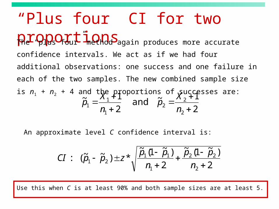
“Plus four” CI for two proportionsThe “plus four” method again produces more accurate confidence

intervals. We act as if we had four additional observations: one

success and one failure in each of the two samples. The new

combined sample size is n1 + n2 + 4 and the proportions of successes

are:

2

1~ and 2

1~

2

22

1

11

n

Xp

n

Xp

An approximate level C confidence interval is:

Use this when C is at least 90% and both sample sizes are at least 5.

2

)~1(~

2

)~1(~*)~~(:

2

22

1

1121

n

pp

n

ppzppCI

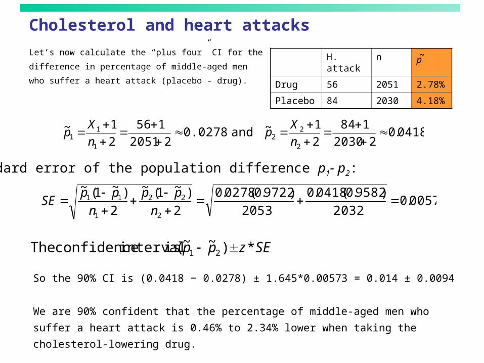
Cholesterol and heart attacks

Let’s now calculate the “plus four” CI for the

difference in percentage of middle-aged men

who suffer a heart attack (placebo – drug).

So the 90% CI is (0.0418 − 0.0278) ± 1.645*0.00573 = 0.014 ± 0.0094

We are 90% confident that the percentage of middle-aged men who suffer a heart

attack is 0.46% to 2.34% lower when taking the cholesterol-lowering drug.

Standard error of the population difference p1- p2:

SEzpp *)~~( is interval confidence The 21

0057.02032

)9582.0(0418.0

2053

)9722.0(0278.0

2

)~1(~

2

)~1(~

2

22

1

11

n

pp

n

ppSE

H. attack n p ̃Drug 56 2051 2.78%

Placebo 84 2030 4.18%

0418.022030

184

2

1~ and 0.027822051

156

2

1~

2

22

1

11

n

Xp

n

Xp

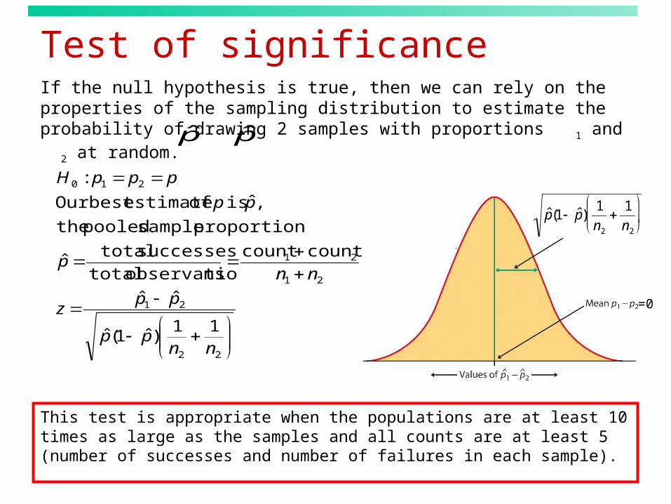
If the null hypothesis is true, then we can rely on the properties of the sampling distribution to estimate the probability of drawing 2 samples with proportions 1 and 2 at random.

Test of significance

This test is appropriate when the populations are at least 10 times as large as the samples and all counts are at least 5 (number of successes and number of failures in each sample).

ˆ p (1 ˆ p )1

n2

1

n2

=0

22

21

21

21

210

11)ˆ1(ˆ

ˆˆ

countcount

nsobservatio total

successes totalˆ

proportion sample pooled the

,ˆ is of estimatebest Our

:

nnpp

ppz

nnp

pp

pppH

p̂ p̂

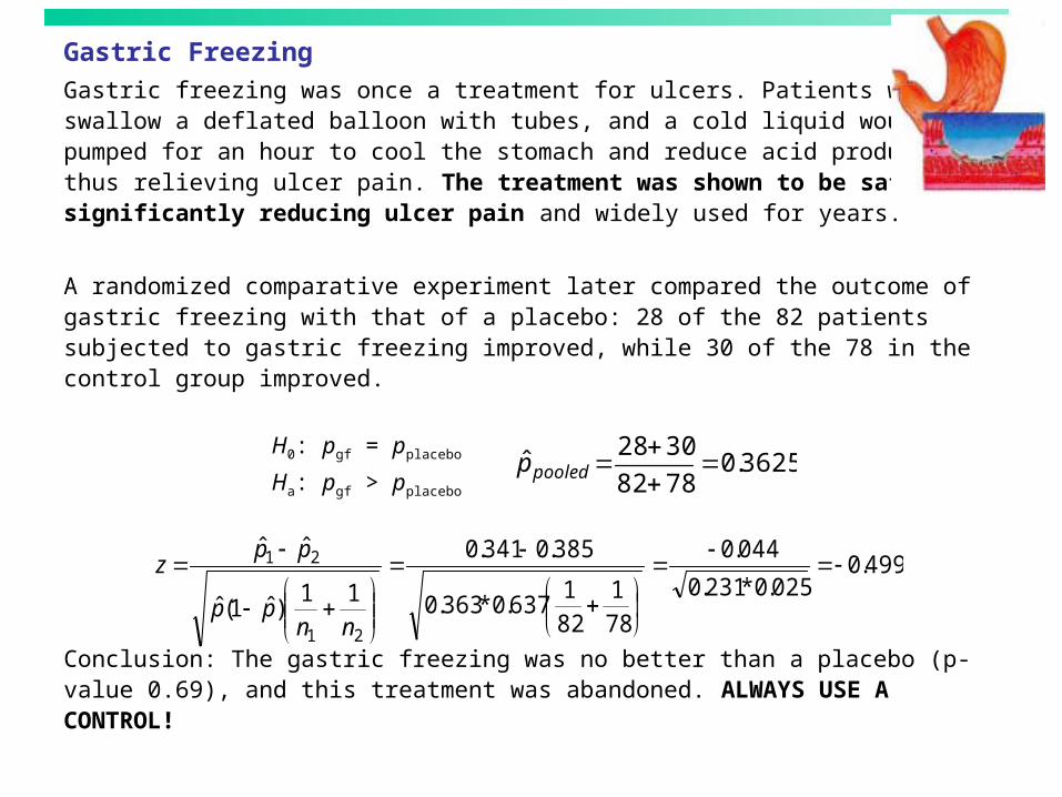
Gastric Freezing

Gastric freezing was once a treatment for ulcers. Patients would swallow a deflated balloon with tubes, and a cold liquid would be pumped for an hour to cool the stomach and reduce acid production, thus relieving ulcer pain. The treatment was shown to be safe, significantly reducing ulcer pain and widely used for years.

A randomized comparative experiment later compared the outcome of gastric freezing with that of a placebo: 28 of the 82 patients subjected to gastric freezing improved, while 30 of the 78 in the control group improved.

Conclusion: The gastric freezing was no better than a placebo (p-value 0.69), and this treatment was abandoned. ALWAYS USE A CONTROL!

H0: pgf = pplacebo

Ha: pgf > pplacebo

499.0025.0*231.0

044.0

78

1

82

1637.0*363.0

385.0341.0

11)ˆ1(ˆ

ˆˆ

21

21

nnpp

ppz

3625.07882

3028ˆ

pooledp

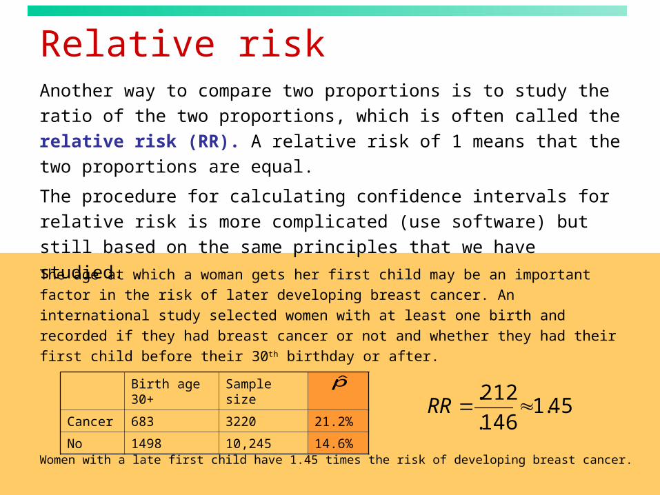
Relative riskAnother way to compare two proportions is to study the ratio of the two

proportions, which is often called the relative risk (RR). A relative risk

of 1 means that the two proportions are equal.

The procedure for calculating confidence intervals for relative risk is

more complicated (use software) but still based on the same principles

that we have studied.

The age at which a woman gets her first child may be an important factor in the

risk of later developing breast cancer. An international study selected women

with at least one birth and recorded if they had breast cancer or not and whether

they had their first child before their 30th birthday or after.

Birth age 30+ Sample size

Cancer 683 3220 21.2%

No 1498 10,245 14.6%

45.1146.

212.RR

Women with a late first child have 1.45 times the risk of developing breast cancer.

p̂