Inf-Sup Conditions for Twofold Saddle Point Problemsnoelw/Noelw/Papers/JhWa09.pdf · · 2009-06-21Inf-Sup Conditions for Twofold Saddle Point Problems ... An application of the

Inf-Sup Conditions for Twofold Saddle Point Problems

Noel J. Walkington1?, Jason S. Howell2??

1 Department of Mathematical Sciences, Carnegie Mellon University, Pittsburgh, PA 15213, e-mail: [email protected] Department of Mathematical Sciences, Carnegie Mellon University, Pittsburgh, PA 15213, e-mail: [email protected]

Submitted to Numerische Mathematik: June 17, 2009

Summary Necessary and sufficient conditions for existence and uniqueness of solutions are devel-oped for twofold saddle point problems which arise in mixed formulations of problems in continuummechanics. This work extends the classical saddle point theory to accommodate nonlinear consti-tutive relations and the twofold saddle structure. Application to problems in incompressible fluidmechanics employing symmetric tensor finite elements for the stress approximation is presented.

Key words saddle point problem – twofold saddle point problem – inf-sup condition – Arnold-Winther element

Mathematics Subject Classification (1991): 65N30

1 Introduction

Many problems in continuous fluid and solid mechanics lead to a variational problems with a saddlepoint structure of the form: (u, p1, p2) ∈ U × P1 × P2, A −BT

1 −BT2

B1 0 0B2 0 0

up1

p2

=

fg1g2

(1.1)

or A 0 −BT1

0 0 −BT2

B1 B2 0

up1

p2

=

fg1g2

. (1.2)

Here U , P1 and P2 are Banach spaces, A : U → U ′ is typically nonlinear, and B1 and B2 are linearoperators. In this paper we develop necessary and sufficient conditions for this class of problems tobe well-posed and consider their numerical approximation.

? Supported in part by National Science Foundation Grants DMS–0811029. This work was also supported by theNSF through the Center for Nonlinear Analysis.?? This material is based upon work supported by the Center for Nonlinear Analysis (CNA) under the NationalScience Foundation Grant No. DMS–0635983.

2 Noel J. Walkington, Jason S. Howell

Problems of type (1.2) can be written as A −BT1 0

B1 0 B2

0 −BT2 0

up2

p1

=

fg2g1

. (1.3)

These problems are often described as twofold saddle point problems due to the nested structurethey exhibit. Each of these problems can be viewed as a single saddle point problem of the form[A −BT

B 0

]=[fg

]where B acts on a product space. The classical theory requires B to satisfy an inf-

sup condition [8,13,14]. The development of discrete spaces which inherit such inf-sup conditionsfor each specific problem is notoriously difficult, and this difficulty is compounded by the productstructure of the twofold saddle point problems. In Lemmas 3.1 and 3.2 we establish necessary andsufficient inf-sup conditions on the constituent operators B1 and B2 to guarantee that the compoundoperator B satisfies inf-sup conditions on the corresponding product space.

The rest of this paper is organized as follows. This introductory section continues with a motivat-ing example, followed by a review of prior results and some notation. Section 2 considers solution ofsingle saddle point problems with nonlinear operator A and their Galerkin approximation. Section3 develops necessary and sufficient conditions on the operators B1 and B2 for problems of type (1.1)and (1.2) to be well posed. An application of the theory is illustrated in Section 4.

1.1 Examples of Twofold Saddle Point Problems

Twofold saddle point problems arise ubiquitously when mixed finite element formulations are usedto approximate the stress in an incompressible fluid or solid [2,9,27,29,24,15,22,23,6,26]. Whenthe usual linear relation S0 = νD(u) for the viscous stress is replaced with a more general relationS0 = νA(D(u)) the equations for the creeping (Stokes) flow of a fluid in a domain Ω ⊂ Rd become,

−div(S) = f , div(u) = 0, S = −pI +A(D(u)).

Here D(u) = (1/2)(∇u+(∇u)T ), S is the stress tensor, and for incompressible fluids takes the formS = −pI +S0 where tr(S0) = 0 is the devatoric part of the stress. If ∂Ω = Γ0∪Γ1 typical boundaryconditions would be

u|Γ0 = u0, Sn|Γ1 = t.

To illustrate our results we review three formulations of this problem:

(1) A single saddle point problem arises when the stress S is eliminated using the constitutive relationas in [30] (classical primal mixed formulation).

(2) Eliminating the gradient of the velocity using the constitutive relation gives rise to a dual mixedvariational formulation [32]. A twofold saddle point problem of the form (1.1) then arises whenthe problem is posed in three variables [9] or the symmetry of the stress tensor is enforced weakly[2].

(3) Alternatively, independent approximation of (the symmetric part of) the velocity gradient givesrise to a twofold saddle problem of the form (1.2) (alternate dual mixed formulation). Dual mixedapproaches that approximate the (nonsymmetric) velocity gradient directly are presented in [24,19].

When the fluid is incompressible the stress-strain relation only acts on the trace free (devatoric)part of the strain. Letting (Rd×d

sym)0 denote the symmetric trace free matrices, we assume

1. A : Rd×d → (Rd×dsym)0.

Inf-Sup Conditions for Twofold Saddle Point Problems 3

2. A(D) = A(Dsym − (tr(D)/d)I).3. The restriction A : (Rd×d

sym)0 → (Rd×dsym)0 is bijective.

Primal Mixed Formulation: The classical weak statement of this problem seeks u−u0 ∈ U =u ∈ H1(Ω)d | u|Γ0 = 0 and p ∈ L2(Ω) satisfying∫

Ω

(A(D(u)) : D(v)− p div(v)

)=∫Ω

f .v +∫Γ1

t.v, v ∈ U,∫Ω

div(u) q = 0, q ∈ L2(Ω).

If Γ1 = ∅, then p, q are required to have average zero. This is a classical saddle point problem takingthe form [

A −div′

div 0

] [up

]=[

f + γ′(t)0

].

Here 〈div′(p),u〉 = (p,div(u)) is the dual operator, and similarly 〈γ′(t),v〉 = (t, γ(v))Γ1 is the dualof the trace operator γ : U → U/H1

0 (Ω)d. Here (·, ·) is the L2(Ω) inner product and 〈·, ·〉 is theinduced duality pairing.

Dual Mixed Formulation: If the inverse of the stress strain relation is available, D(u) =A−1(S), it is possible to write a weak statement that evaluates the stress explicitly. Let

S = S ∈ H(Ω; div)sym | Sn|Γ1 = 0 and U = L2(Ω),

and S(t) be the elements in S ∈ H(Ω; div)sym for which Sn|Γ1 = t. Then (S,u) ∈ S(t)×U satisfies∫Ω

(A−1(S) : T + u.div(T )

)=∫Γ0

u0.Tn, T ∈ S,∫Ω−div(S).v =

∫Ωf.v. v ∈ U.

This weak statement is again a classical saddle point problem. A mixed finite element method forthis formulation in linear elasticity was studied in [3].

If finite element subspaces of H(Ω; div)sym are not available, it is possible to pose the previousweak statement in H(Ω; div) and to use Raviart–Thomas elements. In this instance ∇u = A−1(S)+(∇u)skew. Let

T = S ∈ H(Ω; div) | Sn|Γ1 = 0 and U = (L2(Ω))2,

and T(t) be the elements in S ∈ H(Ω; div) for which Sn|Γ1 = t. Next, define W : Rd → Rd×dskew by

W (w)ij = εijkwk Then (S,u,w) ∈ T(t)× U × L2(Ω) satisfies∫Ω

(A−1(S) : T +W (w) : T + u.div(T )

)=∫Γ0

u0.Tn, T ∈ T,∫Ω−div(S).v =

∫Ωf.v, v ∈ U,∫

Ω−S : W (z) = 0, z ∈ L2(Ω).

This is a twofold saddle point problem taking the form A−1 div′ W−div 0 0−W ′ 0 0

Suw

=

γ′(u0)f0

. (1.4)


Here 〈γ′(u0), T 〉 = (u0, Tn)Γ0 .Finite element methods for the formulation (1.4) arising in linear elasticity were developed by

Arnold, Brezzi, and Douglas [2] (see [6] for a survey of approaches with weakly imposed symmetry).Alternative Dual Mixed Formulation: If the inverse A−1 if the constitutive relation is not

available it is possible to pose a mixed formulation which computes both D(u) and S. Let S andU = L2(Ω)d be as above and

D = D ∈ L2(Ω)d×dsym | tr(D) = 0.

and S(t) be the elements in S ∈ H(Ω; div)sym for which Sn|Γ1 = t. Then (D,u, S) ∈ D× U × S(t)satisfies ∫

ΩA(D) : E − S : E = 0, E ∈ D,∫

Ω(D : T + u.div(T )) =

∫Γ0

u0.Tn, T ∈ S,∫Ω−div(S).v =

∫Ωf.v. v ∈ U.

This is a twofold saddle point problem taking the formA 0 −I0 0 −divI ′ div′ 0

DuS

=

0f

γ′(u0)

. (1.5)

If the trace-free requirement on tensors in D is relaxed a formulation which includes the pressurerequires (D,u, S, p) ∈ L2(Ω)d×dsym × U × S(t)× P satisfying∫

ΩA(D) : E − S : E − pI : E = 0, E ∈ L2(Ω)d×dsym,∫

Ω(D : T + qI : D + u.div(T )) =

∫Γ0

u0.Tn, (T, q) ∈ S× P, (1.6)∫Ω−div(S).v =

∫Ωf.v. v ∈ U.

where P = L2(Ω). This formulation takes the form of (1.5) where the identity operator is replacedwith I × p tr(.).

1.2 Related Results

Problems (1.1) and (1.2) are simplified versions of a full twofold saddle point problem describedby Brezzi and Fortin [14, pp. 41, §II.1]. Existing results regarding different formulations of inf-supconditions for problems of type (1.1) can be found in [28] and [20]. Problems with this structurearise in various applications, including elasticity ([2,6]), complex fluids ([9,20]), and hybridized mixedmethods for second order elliptic problems [18]. Solvability of these problems is usually establishedby showing that A has the required properties and either (i) the combined operator B1 + B2 issurjective or (ii) the operators B1 and B2 individually satisfy appropriate inf-sup conditions.

Problems of type (1.2) are analyzed in a similar manner. In [21] and [25], problems of this typewere treated as nested saddle problems, with the upper left 2 × 2 block of (1.3) being treated asone operator and then showing that block is coercive over the kernel of the operator B2. Sufficient


conditions for solvability and abstract error analysis are also given in [21] and [25]. This theory hasbeen applied to many problems in elasticity and fluids as well, see [27,29,24,15,22,23,26] for someexamples. Problems of type (1.2) were also studied in [16,17]. In these works the twofold saddlepoint problems are treated as single saddle point problems, and solvability is shown by requiringB1 +B2 to satisfy a certain inf-sup condition.

1.3 Notation

For Banach spaces X and Y , X ′ and Y ′ denote their duals, and if F : X → Y is an operator, itsdual operator is denoted by F ′ : Y ′ → X ′ or F T : Y ′ → X ′. If Z ⊂ X is a closed subspace thequotient space is denoted by X/Z and frequently x ∈ X is identified with x + Z ∈ X/Z. The dualspace (X/Z)′ will be identified with the (polar) subspace of X ′,

Z0 = f ∈ X ′ | f(z) = 0, z ∈ Z.

Under this identification ‖f‖(X/Z)′ = ‖f‖X′ .Standard notation is used for the Lebesgue spaces Lp(Ω), the Sobolev spaces W k,p(Ω) and

Hk(Ω) = W k,2(Ω). We will always assume Ω ⊂ Rd is a bounded Lipschitz domain with boundarypartition ∂Ω = Γ0 ∪ Γ1. The inner product L2(Ω) will be denoted as (·, ·). Recall that H(Ω; div) isthe space of vector valued functions in L2(Ω)d having divergence in L2(Ω),

H(Ω; div) = v ∈ L2(Ω)d | div(v) ∈ L2(Ω),

equipped with inner-product

(v, w)H(Ω;div) = (v, w) + (div(v),div(w)).

The space of matrix (tensor) valued functions S ∈ L2(Ω)d×d having divergence div(S) = Sij.j ∈L2(Ω)d is denoted by H(Ω; div) with inner product

(S, T )H(Ω;div) = (S, T ) + (div(S),div(T )).

Matrix valued quantities will be denoted with upper case letters, vectors with bold face lower caseletters.

The Generalized Lax Milgram theorem will be used ubiquitously below. The following is a par-ticularly convenient statement of this fundamental result.

Theorem 1.1 (Generalized Lax Milgram) Let U and V be a Banach spaces, V be reflexive,and c > 0. Let a : U × V → R be bilinear and continuous; that is, there exists C > 0 such that|a(u, v)| ≤ C‖u‖U‖v‖V for all u ∈ U and v ∈ V . Then the following are equivalent:

[C ] (Coercivity) For each u ∈ U ,

sup0 6=v∈V

a(u, v)‖v‖V

≥ c‖u‖U ,

and for each v ∈ V \ 0, supu∈U a(u, v) > 0.[E ] (Existence of Solutions) For each f ∈ V ′ there exists a unique u ∈ U such that

a(u, v) = f(v), ∀ v ∈ V,

and ‖u‖U ≤ (1/c)‖f‖V ′.


[E′

] (Existence of Solutions for the Adjoint Problem) For each g ∈ U ′ there exists a unique v ∈ Vsuch that

a(u, v) = g(u), ∀u ∈ U,

and ‖v‖V ≤ (1/c)‖g‖U ′.

In addition, if U is reflexive then each of the above are equivalent to:

[C′

] (Adjoint Coercivity) For each u ∈ U ,

sup06=u∈U

a(u, v)‖u‖U

≥ c‖v‖V ,

and for each u ∈ U \ 0, supv∈V a(u, v) > 0.

The following classical result for linear saddle point problems is a special case of this theorem.

Corollary 1.1 Let U and P be reflexive Banach spaces and assume that a : U × U → R andb : P × U → R are continuous and bilinear. Then the following are equivalent.

1. (Existence of Solutions) For all f ∈ U ′ and g ∈ P ′ there exists (u, p) ∈ U × P such that

a(u, v)− b(p, v) = f(v), and b(q, u) = g(q),

for all (v, q) ∈ U × P , and there exists C > 0 such that ‖u‖U + ‖p‖P ≤ C(‖f‖U ′ + ‖g‖P ′).2. There exists a constant c > 0 such that

– The restriction a : Z × Z → R is coercive over Z ≡ u ∈ U | b(p, u) = 0, ∀ p ∈ P.

supv∈Z

a(u, v)‖v‖U

≥ c‖u‖U , and supu∈Z

a(u, v) > 0, for all 0 6= v ∈ Z.

– (inf-sup condition) supu∈U

b(p, u)‖u‖U

≥ c‖p‖P .

3. (Coercivity) The bilinear map A((u, p), (v, q)

)= a(u, v)− b(p, v) + b(q, u), is coercive on U ×P :

there exists c > 0 such that

sup(v,q)∈U×P

A((u, p), (v, q)

)‖v‖U + ‖q‖P

≥ c(‖u‖U + ‖p‖P ),

and

sup(u,p)∈U×P

A((u, p), (v, q)

)> 0, for all (0, 0) 6= (v, q) ∈ U × P.

If b : U × P → R satisfies the inf-sup condition in (2) and Z is the kernel, then the restrictionb : U/Z ×P → R satisfies coercivity hypothesis [C] of the Lax Milgram theorem. We make frequentuse of the fact that, in this situation, this implies adjoint coercivity [C

′] as well as existence for both

the primal and dual problem.


2 Nonlinear Saddle Point Problem

Viscoelastic properties of fluids are frequently modeled with a nonlinear constitutive relation. Whenthe fluid is incompressible this gives rise to a saddle point problem of the form; (u, p) ∈ U × P ,

a(u, v)−b(p, v) = f(v),b(q, u) = g(q),

for all (v, q) ∈ U × P , where a : U × U → R is linear in the second argument and b : U × P → R isbilinear. When a(., .) is bilinear the Lax Milgram theorem shows that this problem is well-posed if(and only if) b(., .) satisfies and inf-sup condition and a(., .) is coercive over the kernel of b(., .). Thefollowing theorem is the natural extension of this result to the situation where a(., .) is nonlinear.

Theorem 2.1 Let U and P be reflexive Banach spaces, b : P × U → R be continuous and bilinear,and let a : U ×U → R be linear in its second argument. Let Z = u ∈ U | b(p, u) = 0, ∀ p ∈ P andc > 0. Then the following are equivalent.

1. (Existence of Solutions) For all f ∈ U ′ and g ∈ P ′ there exists (u, p) ∈ U × P such that (a)

a(u, v)− b(p, v) = f(v), and b(q, u) = g(q), (2.1)

for all (v, q) ∈ U × P , and (b) ‖u‖U/Z ≤ (1/c)‖g‖P ′.2.(a) For all f ∈ U ′ and ug ∈ U there exists u ∈ U such that u− ug ∈ Z and

a(u, v) = f(v), v ∈ Z, (2.2)

(b) (inf-sup condition)

supu∈U

b(p, u)‖u‖U

≥ c‖p‖P . (2.3)

Proof When b(., .) is viewed as a bilinear form on P × U/Z the equivalence of statements 1(b) and2(b) follow directly from the Generalized Lax Milgram theorem.

(1)⇒ (2) : Fix f ∈ U ′, ug ∈ U and let (u, p) ∈ U × P satisfying

a(u, v)− b(p, v) = f(v), b(q, u) = b(q, ug), (v, q) ∈ U × P,

with ‖u‖U/Z ≤ (Cb/c)‖ug‖U/Z . Then u− ug ∈ Z so u satisfies 2(a).(2) ⇒ (1) : Fix (f, g) ∈ U ′ × P ′. The Generalized Lax Milgram applied to b : P × U/Z → R

guarantees the existence of ug ∈ U such that b(q, ug) = g(q) and ‖ug‖U/Z ≤ (1/c)‖g‖P ′ . Let u ∈ Usatisfy u− ug ∈ Z and a(u, v) = f(v) for v ∈ Z. Then b(u, q) = g(q),

‖u‖U/Z = ‖ug‖U/Z ≤ (1/c)‖g‖P ′ ,

and a(u, v) − f(v) = 0 for v ∈ Z; that is, a(u, .) − f(.) ∈ (U/Z)′. The Generalized Lax Milgramtheorem applied to b : P × U/Z → R then guarantees the existence of p ∈ P such that

a(u, v)− f(v) = b(p, v), v ∈ U,

which establishes 1(a).

Remarks:

1. Uniqueness of solutions will follow if, for example,

u2 − u1 ∈ Z and a(u2, v)− a(u1, v) = 0, v ∈ Z ⇒ u2 = u1.

2. The above theorem is valid if a : D(A) × U → R has domain strictly contained in U providedthe hypotheses in (1) and (2) require u ∈ D(A).


2.1 Finite Element Approximation

We consider Galerkin approximations of solutions to the saddle point problems in Theorem 2.1.Approximation properties of Galerkin schemes for nonlinear problems depend in a non-trivial fashionupon the structure of the nonlinearity, [10,11]. In this section linearity of the constraints is exploitedto develop some useful formulae for the error. These are then used to develop estimates for the specialcase where the nonlinear operator is strictly monotone and Lipschitz.

Lemma 2.1 Let U and P be reflexive Banach spaces, b : P × U → R be continuous and bilinear,and let a : U ×U → R be linear in its second argument. Let Z = u ∈ U | b(p, u) = 0, ∀ p ∈ P andassume that b(., .) satisfies the inf-sup condition: there exists c > 0 such that

supv∈U

b(p, v)‖v‖U

≥ c‖p‖P .

Fix (f, g) ∈ U ′ × P ′ and suppose that (u, p) ∈ U × P satisfies

a(u, v)− b(p, v) = f(v), b(q, u) = g(q), (v, q) ∈ U × P.

Let Uh ⊂ U and Ph ⊂ P be subspaces and suppose (uh, ph) ∈ Uh × Ph satisfy

a(uh, vh)− b(ph, vh) = f(vh), b(qh, uh) = g(qh), (vh, qh) ∈ Uh × Ph.

Thena(u, vh)− a(uh, vh) = b(p− qh, vh), (vh, qh) ∈ Zh × Ph,

and

‖p− ph‖P ≤ (1 + C/c)‖p− qh‖P + (1/c) supvh∈Uh

a(u, vh)− a(uh, vh)‖vh‖U

, qh ∈ Ph,

where Zh = uh ∈ Uh | b(ph, uh) = 0, ∀ ph ∈ Ph is the discrete null space of b(., .).

Proof The Galerkin orthogonality relations for this problem becomes

a(u, vh)− a(uh, vh)− b(p− ph, vh) = 0, vh ∈ Uh, (2.4)

and (this condition is not used here, see the following lemma)

b(qh, u− uh) = 0, qh ∈ Ph. (2.5)

Restricting the test functions in the first Galerkin orthogonality statement to to vh ∈ Zh shows

a(u, vh)− a(uh, vh) = b(p− qh, vh), (vh, qh) ∈ Zh × Ph.

Using the inf-sup condition on b(., .) we find

‖p− ph‖P ≤ ‖p− qh‖P + ‖qh − ph‖P

≤ ‖p− qh‖P + (1/c) supvh∈Uh

b(qh − ph, vh)‖vh‖U

≤ ‖p− qh‖P + (1/c) supvh∈Uh

b(qh − p+ p− ph, vh)‖vh‖U

≤ (1 + C/c)‖p− qh‖P + (1/c) supvh∈Uh


.


The first statement of this lemma typically gives rise to estimates of the form ‖u− uh‖U ≤C(‖u− vh‖U+‖p− ph‖P ) for all (vh, qh) ∈ Zh×Ph. The proof of this lemma did not use the Galerkinorthogonality relation (2.5) arising from the constraint equation. This relation is used to show thatu−uh satisfies the hypotheses of the following classical result which shows that approximation of uby vh ∈ uh + Zh is optimal.

Lemma 2.2 Let U and P be reflexive Banach spaces and b : P ×U → R be continuous and bilinear,and satisfy the inf-sup condition

supu∈U

b(p, u)‖u‖

≥ cb‖p‖, u ∈ U.

Let Uh ⊂ U and Ph ⊂ P be subspaces and let

Zh = u ∈ U | b(ph, u) = 0, ph ∈ Ph,

andZh = Uh ∩ Zh = uh ∈ Uh | b(ph, uh) = 0, ph ∈ Ph.

Then the following are equivalent.

1. The restriction of b to Uh × Ph satisfies the inf-sup condition,

supuh∈Uh

b(ph, uh)‖uh‖

≥ cb‖ph‖, ph ∈ Ph.

2. There exists C > 0 such that ‖uh‖U/Zh≤ C‖uh‖U/Zh

for all uh ∈ Uh, and

supuh∈Uh

b(ph, uh) > 0, ph 6= 0.

In either case there exists C > 0 such that

infzh∈Zh

‖u− zh‖ ≤ C infvh∈Uh

‖u− vh‖ for all u ∈ Zh.

As stated previously, the form of the error estimates for a specific problem depends upon thestructure of the nonlinear operator a(., .). The following theorem considers the simplest situationwhere the operator is (strictly) maximal monotone and Lipschitz continuous (in which case U istypically a Hilbert space).

Theorem 2.2 Let U and P be reflexive Banach spaces, b : P × U → R be continuous and bilinear,and let a : U × U → R be linear in its second argument. Assume that b(., .) satisfies the inf-supcondition: there exists cb > 0 such that

supv∈U

b(p, v)‖v‖U

≥ cb‖p‖P .

Assume additionally that a(., .) is strictly monotone and Lipschitz in its first argument:

c‖u− v‖2U ≤ a(u, u− v)− a(v, u− v), and a(u,w)− a(v, w) ≤ C‖u− v‖U‖w‖U .

Let Uh ⊂ U and Ph ⊂ P be subspaces and suppose that b : Uh × Ph → R satisfies the inf-supcondition: there exists cb > 0 (independent of h) such that

supvh∈Uh

b(ph, vh)‖vh‖U

≥ cb‖ph‖P .


Fix (f, g) ∈ U ′ × P ′ and suppose that (u, p) ∈ U × P satisfies

a(u, v)− b(p, v) = f(v), b(q, u) = g(q), (v, q) ∈ U × P,

and suppose (uh, ph) ∈ Uh × Ph satisfies

a(uh, vh)− b(ph, vh) = f(vh), b(qh, uh) = g(qh), (vh, qh) ∈ Uh × Ph.

Then there exists a constant C > 0 such that

‖u− uh‖U + ‖p− ph‖P ≤ C

infvh∈Uh

‖u− vh‖U + infqh∈Ph

‖p− qh‖P. (2.6)

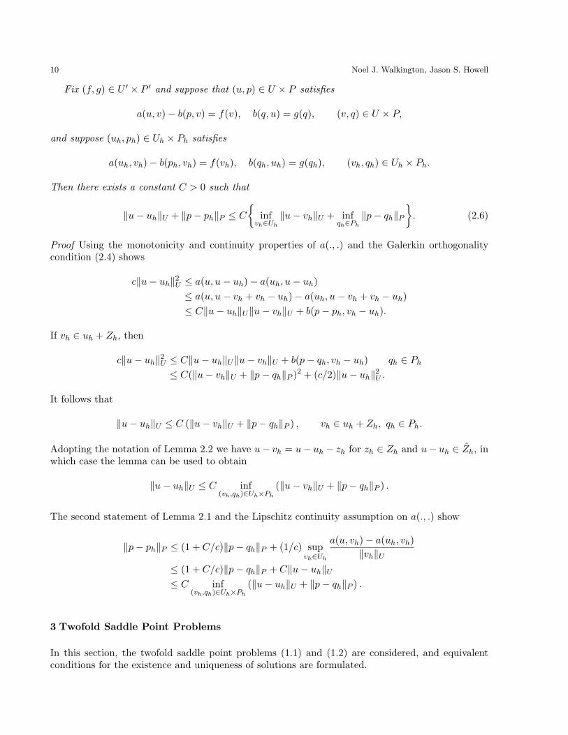
Proof Using the monotonicity and continuity properties of a(., .) and the Galerkin orthogonalitycondition (2.4) shows

c‖u− uh‖2U ≤ a(u, u− uh)− a(uh, u− uh)≤ a(u, u− vh + vh − uh)− a(uh, u− vh + vh − uh)≤ C‖u− uh‖U‖u− vh‖U + b(p− ph, vh − uh).

If vh ∈ uh + Zh, then

c‖u− uh‖2U ≤ C‖u− uh‖U‖u− vh‖U + b(p− qh, vh − uh) qh ∈ Ph≤ C(‖u− vh‖U + ‖p− qh‖P )2 + (c/2)‖u− uh‖2U .

It follows that

‖u− uh‖U ≤ C (‖u− vh‖U + ‖p− qh‖P ) , vh ∈ uh + Zh, qh ∈ Ph.

Adopting the notation of Lemma 2.2 we have u− vh = u− uh − zh for zh ∈ Zh and u− uh ∈ Zh, inwhich case the lemma can be used to obtain

‖u− uh‖U ≤ C inf(vh,qh)∈Uh×Ph

(‖u− vh‖U + ‖p− qh‖P ) .

The second statement of Lemma 2.1 and the Lipschitz continuity assumption on a(., .) show

‖p− ph‖P ≤ (1 + C/c)‖p− qh‖P + (1/c) supvh∈Uh


≤ (1 + C/c)‖p− qh‖P + C‖u− uh‖U≤ C inf

(vh,qh)∈Uh×Ph

(‖u− uh‖U + ‖p− qh‖P ) .

3 Twofold Saddle Point Problems

In this section, the twofold saddle point problems (1.1) and (1.2) are considered, and equivalentconditions for the existence and uniqueness of solutions are formulated.


3.1 Problem Type 1

In this section we consider the twofold saddle problem arising from (1.1): find (u, p1, p2) ∈ U×P1×P2

such that

a(u, v)− b1(p1, v)− b2(p2, v) = f(v) ∀v ∈ U,b1(q1, u) = g1(q1) ∀q1 ∈ P1, (3.1)b2(q2, u) = g2(q2) ∀q2 ∈ P2.

This can be viewed as a single saddle point problem on (P1 × P2)× U with bilinear form

b((p1, p2), u) = b1(p1, u) + b2(p2, u).

The following lemma provides several criteria which guarantee that this bilinear form satisfies theinf-sup condition. Frequently one of these criteria is more readily verified for the discrete spacesused a particular numerical scheme. This lemma extends results in [28] and [20].

Lemma 3.1 Let U , P1, and P2 be reflexive Banach spaces, and let b : P1×U → R, and b2 : P2×U →R be bilinear and continuous. Let

Zbi = v ∈ U | bi(qi, v) = 0∀qi ∈ Pi ⊂ U, i = 1, 2,

then the following are equivalent:

(1) There exists c > 0 such that

supv∈U

b1(p1, v) + b2(p2, v)‖v‖U

≥ c(‖p1‖P1 + ‖p2‖P2) (p1, p2) ∈ P1 × P2


supv∈U

b1(p1, v)‖v‖U

≥ c‖p1‖P1 , p1 ∈ P1 and supv∈Zb1

b2(p2, v)‖v‖U

≥ c‖p2‖P2 , p2 ∈ P2


supv∈Zb2

b1(p1, v)‖v‖U

≥ c‖p1‖P1 , p1 ∈ P1 and supv∈U

b2(p2, v)‖v‖U

≥ c‖p2‖P2 , p2 ∈ P2


supv∈Zb2

b1(p1, v)‖v‖U

≥ c‖p1‖P1 , p1 ∈ P1 and supv∈Zb1

b2(p2, v)‖v‖U

≥ c‖p2‖P2 , p2 ∈ P2.

Proof The result is shown by proving (4) ⇒ (2) ⇒ (1) ⇒ (4) and (4) ⇒ (3) ⇒ (1) ⇒ (4). Theimplications (4)⇒ (2) and (4)⇒ (3) are clear.

As shown in [20], to prove (2)⇒ (1) note that (2) implies the existence of v1 ∈ U with ‖v1‖U = 1and b1(q1, v1) ≥ (c/2)‖q1‖P1 , and the existence of v2 ∈ Zb2 with ‖v2‖U = 1 and b2(q2, v2) ≥(c/2)‖q2‖P2 . Since b2(·, ·) is continuous, there is a C > 0 such that b2(q2, v) ≤ C‖q2‖P2‖v‖U for all(q2, v) ∈ P2 × U . Set u = v1 + (1 + 2C/c)v2. Then ‖u‖U ≤ 2(1 + 2C/c),

b1(q1, u) = b1(q1, v1) ≥ c

2‖q1‖P1 ,


and

b2(q2, u) = b2(q2, v1) +(

1 +2Cc

)b2(q2, v2)

≥ −C‖q2‖P2 +(

1 +2Cc

)c

2‖q2‖P2

=c

2‖q2‖P2 .

Thenb1(q1, u) + b2(q2, u)

‖u‖U≥ c

4(1 + 2C/c)(‖q1‖P1 + ‖q2‖P2

)proving (1). The proof that (3)⇒(1) is similar.

To complete the equivalence, assume (1) and let

Z = Zb1 ∩ Zb2 = u ∈ U | b1(p1, u) + b2(p2, u) = 0, (p1, p2) ∈ P1 × P2.

The generalized Lax Milgram theorem then shows that for each f ∈ (U/Z)′ there exists a unique(p1, p2) ∈ P1 × P2 satisfying

b1(p1, v) + b2(p2, v) = f(v), v ∈ U,

with (‖p1‖P1 + ‖p2‖P2) ≤ (1/c)‖f‖U ′ . Here we identify (U/Z)′ ' f ∈ U ′ | f(u) = 0, u ∈ Z.It follows that for each f ∈ (U/Z)′ there exists p2 ∈ P2 satisfying b2(p2, v) = f(v) for all v ∈ Zb1

with ‖p2‖P2 ≤ (1/c)‖f‖U ′ . The Lax-Milgram condition then shows that b2 is coercive on P2×Zb1/Zso satisfies the inf-sup condition stated in (4).

Similarly for each f ∈ (U/Z)′ there exists p1 ∈ P1 satisfying b1(p1, v) = f(v) for all v ∈ Zb2 with‖p1‖P1 ≤ (1/c)‖f‖U ′ so b1 satisfies the inf-sup condition stated in (4).

Combining Lemma 3.1 and Theorem 2.1 gives necessary and sufficient conditions for twofoldsaddle problem (3.1).

Theorem 3.1 Let U,P1, P2, b1, b2, Zb1 and Zb2 be as in Lemma 3.1, and let Z = Zb1 ∩Zb2. Assumea : U ×U → R is linear in its second argument. Assume that for all f ∈ U ′ and ug ∈ U there existsu0 ∈ Z such that

a(ug + u0, v) = f(v) v ∈ Z,

and that one of the conditions (1)–(4) of Lemma 3.1 are satisfied. Then for all f ∈ U ′, g1 ∈ P ′1, andg2 ∈ P ′2 there exists (u, p1, p2) ∈ U × P1 × P2 satisfying (3.1) with ‖u‖U/Z ≤ C(‖g1‖P ′1 + ‖g2‖P ′2) .

Remark 3.1 Problems of the form

a(u, v)−k∑j=1

bj(pj , v) = f(v),k∑i=1

bi(qi, u) =k∑i=1

gi(qi),

for all (v, q1, . . . , qk) ∈ U × P1 × · · · × Pk are considered in [20] and [28].


3.2 Problem Type 2

We next consider the twofold saddle problems (1.2) and (1.3) corresponding to the variationalproblem (u, p1, p2) ∈ U × P1 × P2,

a(u, v) − b1(p2, v) = f(v) ∀v ∈ U,− b2(p2, q1) = g1(q1) ∀q1 ∈ P1, (3.2)

b1(q2, u) + b2(q2, p1) = g2(q2) ∀q2 ∈ P2.

As indicated in the introduction, two different single saddle problems result with different groupingsof the variables. This gives rise to different, but equivalent, statements of the inf-sup conditionsrequired for the existence of solutions. Different characterizations of the inf-sup condition are usefulwhen constructing numerical schemes since one form is frequently easier to verify than the other.

Define

Zb2 = q2 ∈ P2 | b2(q2, p1) = 0, p1 ∈ P1 and D = u ∈ U | b1(q2, u) = 0, q2 ∈ Zb2.

Grouping the variables as (U × P1)× P2 gives rise to a single saddle problem with operator havingblock form

[A 00 0

]. Coercivity of this operator on Z ⊂ U × P1 will require ‖p1‖P1 ≤ C‖u‖U when

(u, p1) ∈ Z. Alternately stated, Z is the graph of the operator B−12 B1 : D ⊂ U → P1, and the inf-sup

condition on b2 guarantees that this operator is well-defined and continuous. This is the content ofstatement (1) of Lemma 3.2 below.

With the grouping (U × P2) × P1 problem (3.2) has the form of the single saddle problem, thesolution of which requires b2(·, ·) to satisfy an inf-sup condition on P2 and the operator defined bythe block

[A −BT

1B1 0

]must be coercive over U×Zb2 . This latter condition requires b1(., .) to satisfy an

inf-sup condition on Zb2 . These two inf-sup conditions correspond to statement (2) of the followinglemma.

The inf-sup conditions in statement (3) of the lemma arose in one approach to proving an errorestimate for the twofold saddle problem [19]. The first condition gives the existence of a projectionoperator necessary to ensure that the best approximation of (u, p1) can be lifted from the discretekernel Zh to Uh × P1h, while the second condition provides the same lifting for approximations ofp2 from Zb2h to P2h.

Lemma 3.2 Let U,P1, P2 be reflexive Banach spaces, and b1 : P2 × U → R and b2 : P2 × P1 → Rbe bilinear and continuous. Define the bilinear form b : P2 × (U × P1 → R by b(p2, (u, p1)) =b1(p2, u) + b2(p2, p1), and let

Zb2 = q2 ∈ P2 | b2(q2, p1) = 0, p1 ∈ P1,

andZb = (u, p1) ∈ U × P1 | b(p2, (u, p1)) = 0, p2 ∈ P2.

Then the following are equivalent:

(1) There exists a constants C and c > 0 such that

sup(v,q1)∈U×P1

b(p2, (v, q1))‖(v, q1)‖U×P1

≥ c‖p2‖P2 and ‖q1‖P1 ≤ C‖v‖U for (v, q1) ∈ Zb.


supp2∈P2

b2(p2, q1)‖p2‖P2

≥ c‖q1‖P1 , and supv∈U

b1(p2, v)‖v‖U

≥ c‖p2‖P2 , for p2 ∈ Zb2 .



sup(v,q1)∈U×P1

b(p2, (v, q1))‖(v, q1)‖U×P1

≥ c‖p2‖P2 , and supp2∈P2

b2(p2, q1)‖p2‖P2

≥ c‖q1‖P1 .

Moreover, when one of these conditions holds Zb is the graph of a linear function with domain

D = u ∈ U | b1(q2, u) = 0, q2 ∈ Zb2 = u | (u, p1) ∈ Zb.

Remark: The inclusion u | (u, p1) ∈ Zb ⊂ u ∈ U | b1(q2, u) = 0, q2 ∈ Zb2 always holds;the reverse inclusion requires b2 to satisfy an inf-sup condition.

Proof We show (1)⇒ (2)⇒ (3)⇒ (1).(1) ⇒ (2) Setting p2 ∈ Zb2 in the inf-sup condition satisfied by b(., .) immediately gives the

inf-sup condition on b1(., .) sated in (2). To establish the inf-sup condition on b2(., .) use adjointcoercivity of b : P2 × (U × P1)/Zb to obtain

supp2∈P2

b(p2, (u, p1))‖p2‖P2

≥ c‖(u, p1)‖(U×P1)/Zb.

Setting u = 0 and expanding the definition of the quotient norm shows

supp2∈P2

b2(p2, p1)‖p2‖P2

≥ c inf(v,q1)∈Zb

(‖v‖U + ‖p1 − q1‖P1)

≥ (c/C) inf(v,q1)∈Z

(‖q1‖P1 + ‖p1 − q1‖P1)

≥ (c/C)‖p1‖P1 .

The second line follows from the property assumed upon elements of Zb and it was assumed withoutloss of generality that C ≥ 1.

(2)⇒ (3) We first show that for each g2 ∈ P ′2 there exists a solution of (v, q1) ∈ U × P1 of

b(q2, (v, q1)) ≡ b1(q2, v) + b2(q2, q1) = g2(q2), q2 ∈ P2, (3.3)

with c‖(v, q1)‖U×P1 ≤ ‖g2‖P ′2 . The inf-sup assumed on b1(., .) shows that its restriction to b1 :Zb2 × U/D → R is coercive where

D = u ∈ U | b1(q2, u) = 0, q2 ∈ Zb2.

It follows that there exists v ∈ U such that

b1(q2, v) = g2(q2) q2 ∈ Zb2 ,

with c‖v‖U ≤ ‖g2‖P ′2 . Next, the inf-sup condition on b2(·, ·) shows that b2 : P2/Zb2 × P1 → R iscoercive. Since g2(q2)− b1(q2, v) vanishes for q2 ∈ Zb2 there exists a solution q1 of

b2(q2, q1) = g2(q2)− b1(q2, v) q2 ∈ P2,

withc‖q1‖P1 ≤ ‖g2‖+ C‖v‖U ≤ (1 + C/c)‖g2‖P ′2 .

This gives a solution of equation (3.3) with c‖(v, q1)‖U×P1 ≤ ‖g2‖P ′2 .


To establish the inf-sup condition on b in (3), fix p2 ∈ P2 and let g2 ∈ P ′2 satisfy g2(p2) = ‖g1‖2P ′ =‖p2‖2P2

. Then the solution of (3.3) satisfies c‖(v, q1)‖U×P1 ≤ ‖g2‖P ′2 = ‖p2‖P2 and

‖p2‖P2 =g2(p2)‖p2‖P2

=b(p2, (v, q1))‖p2‖P2

≤ b(p2, (v, q1))c‖(v, q1)‖U×P1

.

(3)⇒ (1) Adjoint coercivity of b : P2 × (U × P1)→ R shows

supp2∈P2

b(p2, (v, q1))‖p2‖P2

≥ c‖(v, q1)‖(U×P1)/Zb.

If (v, q1) ∈ Zb it follows that b(p2, (v, q1)) = 0 for all p2 ∈ P2; that is, b2(p2, q1) = −b1(p2, v) for allp2 ∈ P2. The coercivity assumed on b2(., .) then shows

c‖q1‖P1 ≤ supp2∈P2

b2(p2, q1)‖p2‖P2

= supp2∈P2

−b1(p2, v)‖p2‖P2

≤ C‖v‖U .

It follows that problems of the form (3.2) can be treated as single saddle point problems and theapplication of Theorem 2.1 gives rise to necessary and sufficient conditions for existence of solutions.

Theorem 3.2 Let U,P1, P2, b1, b2,D be as in Lemma 3.2 and assume a : U ×U → R is linear in itssecond argument. Assume that for all f ∈ U ′ and ug ∈ U there exists u0 ∈ D such that

a(ug + u0, v) = f(v) v ∈ D,and that one of the conditions (1)–(3) of Lemma 3.2 are satisfied. Then for all f ∈ U ′, g1 ∈ P ′1, andg2 ∈ P ′2 there exists (u, p1, p2) ∈ U × P1 × P2 satisfying (3.2) with ‖u‖U/D ≤ C

(‖g1‖P ′1 + ‖g2‖P ′2

).

4 Application to Problem (1.5)

In this section the saddle point theory developed above is used to solve the nonlinear Stokes problem(1.5) and to formulate numerical schemes to approximate the solution.

Assume Ω ⊂ Rd, d = 2, 3, is bounded and simply connected and ∂Ω = Γ0 ∪ Γ1 is Lipschitz-continuous and the boundary partition is sufficiently regular for classical H2(Ω) regularity to apply.Let

S =S ∈ H(Ω; div)sym | Sn|Γ1 = 0

, U = L2(Ω)d,

D =D ∈ L2(Ω)d×dsym | tr(D) = 0

.

For simplicity we assume a homogeneous traction boundary condition Γ1; non-homogeneous bound-ary data can be accommodated with the usual translation argument. The variational problem is:given f ∈ L2(Ω)d and u0 ∈ H1/2(Γ0)d, find (D,u, S) ∈ D× U × S satisfying∫

ΩA(D) : E − S : E = 0, E ∈ D,∫

Ω−div(S).v =

∫Ωf.v. v ∈ U. (4.1)∫

Ω(D : T + u.div(T )) =

∫Γ0

u0.Tn, T ∈ S,

This problem takes the form of the twofold saddle problem considered in Section 3.2 with operators

a(D,E) =∫ΩA(D) : E, b1(S,E) =

∫ΩS : E, b2(S,v) =

∫Ωdiv(S).v.

Below we will assume |Γ1| 6= 0, otherwise it is necessary to require S ∈ S to satisfy∫Ω tr(S) = 0.


4.1 Solution of the Continuous Problem

Theorem 3.2 will be used to solve problem (4.1) using condition (2) of Lemma 3.2 to establish theinf-sup hypotheses.

First Inf-Sup Condition: The inf-sup condition on b2(., .) becomes

supS∈S

∫Ω div(S).v‖S‖H(Ω;div)

≥ c‖v‖L2(Ω), ∀v ∈ U. (4.2)

A proof of this inequality may be found in [12, §11.1, 11.2]. Briefly, given v ∈ U select S = D(u) ≡(1/2)(∇u + (u)T ) where u is the solution of the linear elasticity problem,

div(D(u)) = v, u|Γ0 = 0, D(u)n|Γ1 = 0.

Then∫Ω div(S).v = ‖v‖2L2(Ω) the Poincare and Korn inequalities may be used to verify that there

exists C > 0 such that ‖S‖H(Ω;div) ≤ C‖v‖L2(Ω), and (4.2) follows. For the discrete problem we use

the property that regularity theory for the linear elastic problem shows that if v ∈ L2(Ω)d thenu ∈ H2(Ω)d so S = D(u) ∈ H1(Ω)d×d.

Second Inf-Sup Condition: Setting Zb2 = S ∈ S | divS = 0, the inf-sup condition requiredof b1(., .) becomes

supD∈D

∫ΩD : S‖D‖L2(Ω)

≥ c‖S‖L2(Ω), ∀S ∈ Zb2 . (4.3)

Given S ∈ Zb2 the inf-sup condition is established upon setting D = S − (1/e)tr(S) ∈ D to obtain∫ΩD : S = ‖D‖2L2(Ω). Lemma A.2 in the appendix shows that there is a constant C > 0 such that‖S‖L2(Ω) ≤ C‖D‖L2(Ω) when S ∈ Zb2 and (4.3) follows.

Define the set

D =D ∈ D |

∫ΩD : S = 0 ∀S ∈ Zb2

⊂ D.

This set is not easily characterized so minimal conditions onA : Rd×d → Rd×d to guarantee coercivityover D are not available. Fortunately A is typically a maximal monotone operator on all of Rd×d sothis is not an issue. Granted this, Theorem 3.2 establishes existence of solutions to problem (4.1).

Theorem 4.1 Let Ω ⊂ Rd and the spaces S, U , and D be given at the beginning of this section.Assume A : Rd×d → Rd×d maps bounded sets to bounded sets, and satisfies

(A(E)−A(D)) : (E −D) ≥ 0 and lim|D|→∞

A(D) : D/|D| → ∞.

Then for all f ∈ L2(Ω)d and u0 ∈ H1/2(Γ0)d, problem (4.1) has a solution (D,u, S) ∈ D × U × Ssatisfying

‖D‖D/D ≤ C(‖f‖L2(Ω) + ‖u0‖H1/2(Γ0)

),

whereD = D ∈ D |

∫ΩD : S = 0, ∀S ∈ S with div(S) = 0.

Moreover, if A is strictly monotone,

(A(E)−A(D)) : (E −D) > 0, E 6= D,

the solution is unique.


Fig. 4.1. Lowest–order Arnold–Winther elements in two dimensions for Sh (left) and uh (right). For Sh, the pointsrepresent values of the components of Sh (vertices) and the value of the three components of the moment of degree 0of Sh (interior), and the arrows represent the values of the moments of degree 0 and 1 of the two normal componentsof Shon each edge. For uh, the points represent the value of of the two components at the three interior nodes.

4.2 Galerkin Approximation

Let Thh>0 be a regular family of triangulations of Ω and let Dh, Uh, Sh be finite dimensionalsubspaces of D, U, S, respectively. We consider Galerkin approximations of problem (4.1) satisfying(Dh,uh, Sh) ∈ Dh × Uh × Sh,∫

ΩA(Dh) : Eh − Sh : Eh = 0, Eh ∈ Dh,∫

Ω−div(Sh).vh =

∫Ωf.vh, vh ∈ Uh, (4.4)∫

Ω(Dh : Th + uh.div(Th)) =

∫Γ0

u0.Thn, Th ∈ Sh,

In this context establishing discrete versions of (4.2) and (4.3) can be considerably less compli-cated and technical than showing a condition of the form

sup(Dh,uh)∈Dh×Uh

∫Ω (Dh : Th + uh.div(Th))‖Dh‖D + ‖uh‖U

≥ c‖Th‖H(Ω;div),

since the discrete form of (4.3) only needs to be verified for divergence free Th.First Inf-Sup Condition: The issue of finding conforming finite elements for symmetric tensors

satisfying an inf-sup condition of the form (4.2) is well-documented ([14,32,4,5]). We consider thefinite element pairs (Sh, Uh) of symmetric tensors and vectors constructed by Arnold and Winther[7,1] which satisfy the inf-sup condition.

Let k ≥ 1 and define Pk(K) to be the set of all polynomials of degree at most k on the simplexK ∈ Th. On K, define SK to be the symmetric Arnold-Winther tensors

SK =Sh ∈ H(div,K)sym | Sh ∈ (Pk+d(K))d×dsym and div(Sh) ∈ (Pk(K)

.

The space Sh is the union of SK over all K ∈ Th, subject to the condition that the normal componentsare continuous across mesh edges (faces for d = 3) and all components are continuous at vertices.Define

Uh =

u ∈ L2(Ω)d | u|K ∈ Pk(K) ∀K ∈ Th

and note that there is no interelement continuity requirement for Uh. Figure 4.1 gives a diagram ofthe degrees of freedom on each triangle for the lowest order Arnold-Winther (Sh, uh) pair (k = 1) intwo dimensions. In [7,1] an interpolation operator Πh : S∩H1(Ω)d×d → Sh is constructed for which


div(ΠhS) = PUh div(S),

S ∩H1(Ω)d×d div−−−−→ U

Πh

y yPUh

Shdiv−−−−→ Uh

where is the orthogonal projection PUh : U → Uh and s > 0.The discrete analog of (4.2) follows since for any vh ∈ Uh there is a S ∈ S∩H1(Ω)d×d satisfying

div(S) = vh and ‖S‖L2(Ω) ≤ C‖vh‖L2(Ω). Then div(ΠhS) = PUh div(S) = vh and ‖ΠhS‖H(Ω;div) ≤C‖vh‖U and the discrete inf-sup condition follows.

Second Inf-Sup Condition: The commuting diagram for the Arnold Winther spaces shows

Zh ≡Sh ∈ Sh |

∫Ω

div(Sh).uh = 0, uh ∈ Uh

= Sh ∈ Sh | div(Sh) = 0

The second inf-sup condition for the discrete spaces becomes

supDh∈Dh

∫ΩDh : Sh‖Dh‖L2(Ω)

≥ c‖Sh‖L2(Ω), Sh ∈ Zh. (4.5)

When div(S) = 0, Lemma A.2 of the appendix shows that ‖S‖L2(Ω) ≤ C‖S0‖L2(Ω) where S0 =S − (tr(S)/d)I is the trace free part of S. Since Sh ∈ Sh is piecewise polynomial of degree k + d onTh, so it suffices to let

Dh =Dh ∈ L2(Ω)d×d | tr(Dh) = 0 and Dh|K ∈ Pk+d(K)d×d, K ∈ Th

;

however, typically much smaller spaces (and hence cheaper numerical schemes) suffice. Note toothat smaller spaces will not necessarily result in a loss of accuracy. For smooth functions the ArnoldWinther spaces exhibit the following approximation properties,

‖S −ΠhS‖H(div;Ω) ≤ Chk+1

‖u− PUh u‖L2(Ω) ≤ Chk+1,

and this rate would be achieved for ‖Dh −D‖L2(Ω) if Dh contained the piecewise polynomials ofdegree k.

Having constructed discrete subspaces which satisfy these inf-sup conditions, Theorem 2.2 pro-vides error estimates for the Galerkin approximations.

Theorem 4.2 Let Ω ⊂ Rd and the spaces S, U , and D be given at the beginning of this section.Assume there exist constants C, c > 0 such that A : Rd×d → Rd×d satisfies

c|D − E|2 ≤ (A(E)−A(D)) : (E −D) and (A(E)−A(D)) : F ≤ |E −D| |F |.

Let Thh>0 be a regular family of triangulations of Ω, Sh ⊂ S be the Arnold Winther space of indexk over Th, Uh ⊂ U be the discontinuous piecewise polynomial space of degree k, and Dh ⊂ D be thediscontinuous piecewise polynomial space of degree k + d.

Let (D,u, S) satisfy (4.1) and (Dh,uh, Sh) satisfy (4.4). Then there is a constant c > 0 suchthat, for 1 ≤ m ≤ k + 1,

‖D −Dh‖D + ‖u− uh‖U + ‖S − Sh‖S ≤ Chm‖D‖m + ‖u‖m + ‖S‖m + ‖div(S)‖m

.


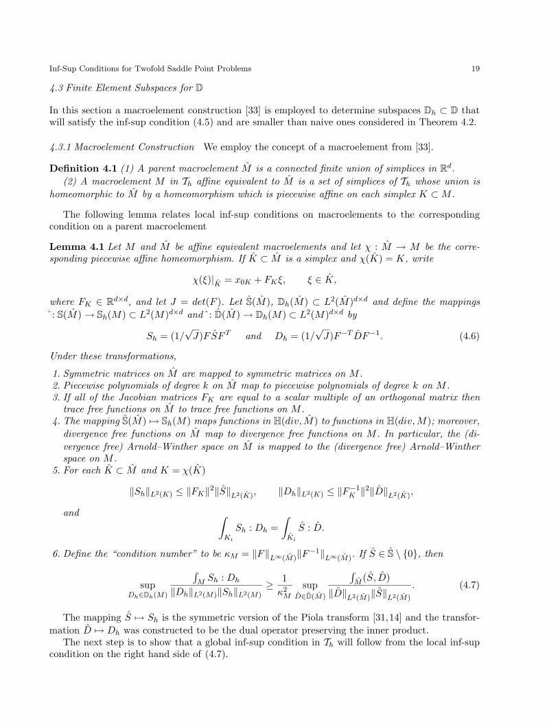
4.3 Finite Element Subspaces for D

In this section a macroelement construction [33] is employed to determine subspaces Dh ⊂ D thatwill satisfy the inf-sup condition (4.5) and are smaller than naive ones considered in Theorem 4.2.

4.3.1 Macroelement Construction We employ the concept of a macroelement from [33].

Definition 4.1 (1) A parent macroelement M is a connected finite union of simplices in Rd.(2) A macroelement M in Th affine equivalent to M is a set of simplices of Th whose union is

homeomorphic to M by a homeomorphism which is piecewise affine on each simplex K ⊂M .

The following lemma relates local inf-sup conditions on macroelements to the correspondingcondition on a parent macroelement

Lemma 4.1 Let M and M be affine equivalent macroelements and let χ : M → M be the corre-sponding piecewise affine homeomorphism. If K ⊂ M is a simplex and χ(K) = K, write

χ(ξ)|K = x0K + FKξ, ξ ∈ K,

where FK ∈ Rd×d, and let J = det(F ). Let S(M), Dh(M) ⊂ L2(M)d×d and define the mappingsˆ: S(M)→ Sh(M) ⊂ L2(M)d×d andˆ: D(M)→ Dh(M) ⊂ L2(M)d×d by

Sh = (1/√J)FSF T and Dh = (1/

√J)F−T DF−1. (4.6)

Under these transformations,

1. Symmetric matrices on M are mapped to symmetric matrices on M .2. Piecewise polynomials of degree k on M map to piecewise polynomials of degree k on M .3. If all of the Jacobian matrices FK are equal to a scalar multiple of an orthogonal matrix then

trace free functions on M to trace free functions on M .4. The mapping S(M) 7→ Sh(M) maps functions in H(div, M) to functions in H(div,M); moreover,

divergence free functions on M map to divergence free functions on M . In particular, the (di-vergence free) Arnold–Winther space on M is mapped to the (divergence free) Arnold–Wintherspace on M .

5. For each K ⊂ M and K = χ(K)

‖Sh‖L2(K) ≤ ‖FK‖2‖S‖L2(K), ‖Dh‖L2(K) ≤ ‖F−1K ‖

2‖D‖L2(K),

and ∫Ki

Sh : Dh =∫Ki

S : D.

6. Define the “condition number” to be κM = ‖F‖L∞(M)‖F−1‖L∞(M). If S ∈ S \ 0, then

supDh∈Dh(M)

∫M Sh : Dh

‖Dh‖L2(M)‖Sh‖L2(M)≥ 1κ2M

supD∈D(M)

∫M (S, D)

‖D‖L2(M)‖S‖L2(M)

. (4.7)

The mapping S 7→ Sh is the symmetric version of the Piola transform [31,14] and the transfor-mation D 7→ Dh was constructed to be the dual operator preserving the inner product.

The next step is to show that a global inf-sup condition in Th will follow from the local inf-supcondition on the right hand side of (4.7).


Theorem 4.3 Let M be a family of parent macroelements and Ω = ∪HMH be a covering of Ωby macroelements of Th each affine equivalent to some M ∈ M. For each M ∈ M let D(M),S(M) ⊂ L2(M)d×d be specified and assume that there exists c > 0

supD∈D(M)

∫M (S, D)

‖D‖L2(M)

≥ c‖S‖L2(M), S ∈ S(M), M ∈ M.

Let Sh ⊂ L2(Ω)d×d and assume that the local spaces Sh(M) formed by restriction to M are theimages of S(M) under the (symmetric) Piola transform (4.6). If Dh is the (discontinuous) finiteelement space on Th spanned by the local spaces Dh(M), then

supDh∈Dh

∫ω Sh : Dh

‖Dh‖L2(Ω)≥ c

γκ2‖Sh‖L2(Ω),

where κ = maxM κM is the maximal condition number on each macroelement and γ is the ply of thecovering Ω = ∪HMH ; that is, x ∈ Ω belongs to at most γ macroelements.

Proof Fix Sh ∈ Sh and for each H let DH ∈ Dh(MH) satisfy ‖DH‖L2(MH) = ‖Sh‖L2(MH) and∫MH

DH : Sh ≥ (c/κ2)‖Sh‖2L2(MH).

Then define Dh =∑

H DH , and use the property that MH cover Ω to conclude∫ΩDh : Sh ≥ (c/κ2)‖Sh‖2L2(Ω).

Next, since the covering has finite ply we compute

‖Dh‖2L2(Ω) =∑K∈Th

∫K

∣∣∣∣∣∣∑

H:K⊂MH

DH

∣∣∣∣∣∣2

≤∑K∈Th

∫Kγ

∑H:K⊂MH

|DH |2

= γ∑K∈Th

∑H:K⊂MH

∫K|DH |2

= γ∑H

∑K⊂MH

∫K|DH |2

= γ∑H

∫MH

|DH |2

= γ∑H

∫MH

|Sh|2

≤ γ2

∫Ω|Sh|2.

It follows that ‖Dh‖L2(Ω) ≤ γ‖Sh‖L2(Ω), and∫ΩDh : Sh‖Dh‖L2(Ω)

≥ (c/γκ2)‖Sh‖L2(Ω).


θ

hM

x0

x2

x3

x1

K1

K21

K1

K2

0

x2

x1

χM

MM

Fig. 4.2. Reference M and affine equivalent M macroelements.

In practice it is trivial to construct a covering of Ω by macroelements with finite ply, and a boundupon the condition number follows from the bound upon the aspect ratio of the simplices in Th. Inthis situation the global inf-sup condition will follow provided the local inf-sup condition holds oneach parent macroelement with constant independent of M ∈ M. The following lemma shows thatverification of the inf-sup condition on each macroelement reduces to linear algebra.

Lemma 4.2 Let M be a parent macroelement and suppose D, S ⊂ L2(M)d×dsym are finite dimensionalsubspaces and that for all S ∈ S∫

MD : S = 0 ∀D ∈ D ⇒ S = 0.

Then there exists c > 0 such that

supD∈D

∫M D : S

‖D‖L2(M)

≥ c‖S‖L2(M), S ∈ S. (4.8)

Proof Let the linear map φ : D → S be characterized by (φ(D), S)L2 = (D, S)L2 for all S. Thehypothesis of the theorem shows Rg(φ)⊥ = 0, and finite dimensionality guarantees Rg(φ) is closedso is all of S. Then φ is surjective and is an isomorphism on Ker(φ)⊥. Selecting D = φ−1(S) ∈Ker(φ)⊥ establishes the inf-sup condition (4.8).

If M is finite the inf-sup condition then reduces to linear algebra. When M is infinite themacroelements can usually be parameterized by a compact set; for example, the vertices if the sim-plices on M typically lie in a compact set of Rd. If the constants c = c(M) > 0 depend continuouslyupon the parameters a uniform bound from below will follow (positive functions on compact setsachieve their minimum).


(1, 0)(0, 0)

α

α α

x1

K1

Fig. 4.3. If K1 has minimum angle α then x1 lies in a compact subset of R2.

4.3.2 Two Dimensional Example In this section the macroelement technique is used to show thatin two dimensions the inf-sup condition (4.5) holds for the lowest order Arnold Winther elements,k = 1, when Dh is the space of discontinuous “quadratic plus bubble” symmetric trace free matrices.For this purpose we select the macroelements to be pairs of triangles which have an edge in common,and the reference macro elements be pairs of simplices with common edge lying on the unit intervalof the x-axis (see Figure 4.2),

M = M = K1 ∪ K2 | K1 ∩ K2 = [0, 1]× 0, and K1, K2 have aspect ratio bounded by C.

If Th is a regular family of triangulations of Ω then each pair of triangles M = K1 ∪K2 sharingan edge of length hM can be mapped to M ∈ M with an affine homeomorphism of the form,

x = χ(x) = x0 + hMQx, QTQ = I.

Selecting the Jacobians to be orthogonal guarantees that trace free matrices are mapped to tracefree matrices under the Piola transformations (4.6), and that condition numbers κM = 1 are triviallybounded.

It remains to verify the inf-sup condition on each macroelement M ∈ M. To do this we param-eterize M = K1 ∪ K2 ∈ M by the coordinates of the vertices x1 and x2 of K1 and K2 not on thex1-axis. Since each simplex has bounded aspect ratio it follows that the pair (x1, x2) lie in a compactsubset of R2 as indicated in Figure 4.3. Moreover, since the inf-sup condition only involves integralsover M = M(x1, x2) it is clear that the constant depends continuously upon the two parameters.In this situation it suffices to establish the inf-sup condition on each M(x1, x2) using, for example,Lemma 4.2.

The linear algebra required to complete the proof of the inf-sup condition involves large matriceswith symbolic components, (x1, x2). Maple was used to verify the hypothesis in Lemma 4.2 asfollows:

1. On each of K1 and K2 the divergence free functions in the lowest order Arnold–Winther spacetake the form

S11 = 1/2 a0x2 + 1/6 a1x

3 + 1/2 a2yx2 +

(a3 + a4y + a5y

2)x+ a6 + a7y + a8y

2 + a9y3

S12 = −a0xy − 1/2 a1x2y − 1/2 a2y

2x− a3y − 1/2 a4y2 − 1/3 a5y

3

−a10x− 1/2 a11x2 − 1/3 a12x

3 + a17

S22 = 1/2 a0y2 + 1/2 a1xy

2 + 1/6 a2y3 +

(a10 + a11x+ a12x

2)y + a13 + a14x+ a15x

2 + a16x3


2. Accumulate the set of equations to enforce the following:(a) S is continuous at the vertices (0, 0) and (1, 0),

S(0, 0−) = S(0, 0+), and S(1, 0−) = S(1, 0+).

(b) Sn is continuous across the x-axis where n = (0, 1)T . Along the x-axis the normal componentsare univariate polynomials of degree three which agree at the end points, so it suffices to requirecontinuity at two more points.

S(1/3, 0−)n = S(1/2, 0+)n, and S(2/3, 0−)n = S(2/3, 0+)n.

(c) On each of the triangles, Ki, S is orthogonal to a basis of the trace free matrices withcomponents in P2(Ki)⊕ bKi

.

∫Ki

(S11 − S22

)p = 0,

∫Ki

S12p = 0, p ∈ 1, x, y, x2, xy, y2, bKi(x, y).

3. Solve the system of linear equations. If the solution is a constant diagonal matrix, S(x, y) = αI,conclude the inf-sup condition holds. Since the coefficient matrix of the linear system has symbolicentries corresponding to the components of x1 and x2 fraction free Gauss elimination should beemployed for their solution.

Granted the integrity of the linear algebra system, this procedure provides a proof of the followinglemma.

Lemma 4.3 Let Thh>0 be a regular family of triangulations of a bounded domain Ω ⊂ R2 and letZh ⊂ Sh be the subspace of the lowest order (k = 1) Arnold-Winther tensors with divergence zeroand let

Dh = D ∈ D | Dij |K ∈ P2(K)⊕ bK ∀K ∈ Th .

Then there is a constant c > 0 independent of h such that

supDh∈Dh

∫Ω Dh : Sh‖Dh‖D

≥ c‖Sh‖, Sh ∈ Zh.

The bubble component was necessary for the two element macroelement construction. However,numerical experiments suggest that it may not be required if a larger macroelement is used. Forexample, if Ω is a square (or L-shaped etc.) and is triangulated by dividing uniform square gridsalong the diagonal, then groups of 8 triangles (four squares) can be mapped to the macroelementshown in Figure 4.4(a) by maps of the form x = χM (x) = x0 +hξ so that the Jacobian is F = hI. Inthis situation the linear system only contains numerical entries, and the macroelement calculationsshows that the bubble is not required; that is the inf-sup condition is satisfied when

Dh = D ∈ D | Dij |K ∈ P2(K) ∀K ∈ Th .


(a) Eight triangle macroele-ment

(b) Four triangle macroele-ment

Fig. 4.4. Parent macroelements used for inf-sup conditions for the trace-free D formulation (a) and for the formulationwith pressure (b).

4.4 Alternate Formulation with Pressure

The solution (1.6) requires

supD∈D

∫ΩD : S + pI : D

‖D‖≥ c(‖S‖S + ‖p‖P ) , ∀(S, p) ∈ Z × P. (4.9)

The proof of (4.9) is shown by setting D = S−(1/e)tr(S) (as for (4.3)) if ‖S‖S ≥ ‖p‖P and choosingD = pI − S when ‖S‖S ≤ ‖p‖P .

The macroelement construction is vastly simplified in this situation since the mappings χ : M →M do not need to preserve the trace. In particular, a single parent element suffices and the inf-sup condition reduces to showing a single (numerical) matrix has full rank. For the parent elementwith four triangles shown in Figure 4.4(b), the macroelement construction shows that the inf-supcondition (4.9) is satisfied when Sh and Uh are as in Section 4.2, and

Dh =D ∈ L2(Ω)d×dsym | Dij |K ∈ P1(K)⊕ bK ∀K ∈ Th

,

and

Ph = p ∈ P | p|K ∈ P1(K)⊕ bK ∀K ∈ Th .

If PDh and PPh denote the orthogonal projections, onto these spaces we have

‖D − PDhD‖L2(Ω) ≤ chm‖D‖m , 0 ≤ m ≤ 2,

‖p− PPh p‖L2(Ω) ≤ chm‖p‖m , 0 ≤ m ≤ 2.

The error estimate for the discrete problem becomes

‖D −Dh‖D + ‖u− uh‖U + ‖S − Sh‖S + ‖p− ph‖P

≤ Chm‖D‖m + ‖u‖m + ‖S‖m + ‖div(S)‖m + ‖p‖m

.


A Auxiliary Results

Lemma A.1 Let Ω ⊂ Rd be a bounded Lipschitz domain and let ∂Ω = Γ0 ∪ Γ1 be a decompositioninto two open sets with |Γ1| 6= 0. Let U = u ∈ H1(Ω)d | u|Γ0 = 0. Then there exists c > 0 suchthat

supu∈U

∫Ω p div(u)‖u‖H1(Ω)

≥ c‖p‖L2(Ω), p ∈ L2(Ω).

Proof Recall that

supu0∈H1

0 (Ω)d

∫Ω p div(u0)‖u0‖H1(Ω)

≥ c0‖p‖L2(Ω)/R,

and ‖p‖2L2(Ω) = ‖p‖2L2(Ω)/R + |Ω|p2 = ‖p− p‖2L2(Ω) + |Ω|p2 where p is the average value of p. Let

U = H10 (Ω)d⊕U1 be the orthogonal decomposition. Then writing u ∈ U as u = u0 +u1 we compute∫

Ωpu =

∫Ω

(p− p) div(u0 + u1) + p div(u1)

=∫Ω

(p− p) div(u0 + u1) + p

∫Γ1

u1.n.

Since the trace operator γ : U → H1/2(Γ1) is surjective, there exists u1 ∈ U1 with ‖u1‖H1(Ω) = 1such that the integral on the right is positive. Then∫

Ωpu ≥

∫Ω

(p− p) div(u0)− ‖p− p‖L2(Ω) + c1|p|

≥ (c0‖u0‖ − 1)‖p− p‖L2(Ω) + c1|p|= (c0‖u0‖ − 1)‖p‖L2(Ω)/R + c1|p|.

Selecting ‖u0‖ = (1 + c1)/c0 gives ‖u‖ ≤ C(c0, c1) which completes the proof.

Lemma A.2 Let Ω ⊂ Rd be a bounded Lipschitz domain and let ∂Ω = Γ0 ∪ Γ1 be a decompositioninto two open sets with |Γ1| 6= 0. Let S = S ∈ H(div;Ω) | Sn|Γ1 = 0 and U = u ∈ H1(Ω)d |u|Γ0 = 0. Then there exists c > 0 such that

‖tr(S)‖L2(Ω) ≤ C(‖S0‖L2(Ω) + ‖div(S)‖U ′

),

where S0 = S − (tr(S)/d)I is the deviatoric part of S.

Proof Let (u, p) ∈ U × L2(Ω) satisfy

(u,v)H1(Ω) + (p, div(v))L2(Ω) = 0, (div(u), q)L2(Ω) = (tr(S), q)L2(Ω),

for all (v, q) ∈ U × L2(Ω). The previous lemma shows that the inf-sup condition is satisfied, sosolutions exists and ‖u‖H1(Ω) ≤ C‖tr(S)‖L2(Ω). Then

‖tr(S)‖2L2(Ω) =∫Ωtr(S) div(u)

=∫Ωtr(S)I : (∇u)

= d

∫Ω

(S − S0) : (∇u)

= −d∫Ωdiv(S).u + S0 : (∇u)

≤ d(‖div(S)‖2U ′ + ‖S0‖2L2(Ω)

)1/2‖u‖H1(Ω).


In the third line we used the identity (1/d)tr(S)I = S − S0, and the fourth line follows since Sn.uvanishes on the boundary.

References

1. D. N. Arnold, G. Awanou, and R. Winther. Finite elements for symmetric tensors in three dimensions. Math.Comp., 77(263):1229–1251, 2008.

2. D. N. Arnold, F. Brezzi, and J. Douglas, Jr. PEERS: a new mixed finite element for plane elasticity. Japan J.Appl. Math., 1(2):347–367, 1984.

3. D. N. Arnold, J. Douglas, Jr., and C. P. Gupta. A family of higher order mixed finite element methods for planeelasticity. Numer. Math., 45(1):1–22, 1984.

4. D. N. Arnold, R. S. Falk, and R. Winther. Differential complexes and stability of finite element methods. I. The deRham complex. In Compatible spatial discretizations, volume 142 of IMA Vol. Math. Appl., pages 24–46. Springer,New York, 2006.

5. D. N. Arnold, R. S. Falk, and R. Winther. Differential complexes and stability of finite element methods. II.The elasticity complex. In Compatible spatial discretizations, volume 142 of IMA Vol. Math. Appl., pages 47–67.Springer, New York, 2006.

6. D. N. Arnold, R. S. Falk, and R. Winther. Mixed finite element methods for linear elasticity with weakly imposedsymmetry. Math. Comp., 76(260):1699–1723 (electronic), 2007.

7. D. N. Arnold and R. Winther. Mixed finite elements for elasticity. Numer. Math., 92(3):401–419, 2002.8. I. Babuska. The finite element method with Lagrangian multipliers. Numer. Math., 20:179–192, 1972/73.9. J. Baranger, K. Najib, and D. Sandri. Numerical analysis of a three-fields model for a quasi-Newtonian flow.

Comput. Methods Appl. Mech. Engrg., 109(3-4):281–292, 1993.10. J. W. Barrett and W. B. Liu. Finite element error analysis of a quasi-Newtonian flow obeying the Carreau or

power law. Numer. Math., 64(4):433–453, 1993.11. J. W. Barrett and W. B. Liu. Quasi-norm error bounds for the finite element approximation of a non-Newtonian

flow. Numer. Math., 68(4):437–456, 1994.12. S. C. Brenner and L. R. Scott. The mathematical theory of finite element methods, volume 15 of Texts in Applied

Mathematics. Springer-Verlag, New York, second edition, 2002.13. F. Brezzi. On the existence, uniqueness and approximation of saddle-point problems arising from Lagrangian

multipliers. Rev. Francaise Automat. Informat. Recherche Operationnelle Ser. Rouge, 8(R-2):129–151, 1974.14. F. Brezzi and M. Fortin. Mixed and hybrid finite element methods, volume 15 of Springer Series in Computational

Mathematics. Springer-Verlag, New York, 1991.15. R. Bustinza, G. N. Gatica, M. Gonzalez, S. Meddahi, and E. P. Stephan. Enriched finite element subspaces for

dual-dual mixed formulations in fluid mechanics and elasticity. Comput. Methods Appl. Mech. Engrg., 194(2-5):427–439, 2005.

16. Z. Chen. Analysis of expanded mixed methods for fourth-order elliptic problems. Numer. Methods PartialDifferential Equations, 13(5):483–503, 1997.

17. Z. Chen. Expanded mixed finite element methods for linear second-order elliptic problems. I. RAIRO Model.Math. Anal. Numer., 32(4):479–499, 1998.

18. B. Cockburn and J. Gopalakrishnan. Error analysis of variable degree mixed methods for elliptic problems viahybridization. Math. Comp., 74(252):1653–1677 (electronic), 2005.

19. V. J. Ervin, J. S. Howell, and I. Stanculescu. A dual-mixed approximation method for a three-field model of anonlinear generalized Stokes problem. Comput. Methods Appl. Mech. Engrg., 197(33-40):2886–2900, 2008.

20. V. J. Ervin, E. W. Jenkins, and S. Sun. Coupled generalized non-linear Stokes flow with flow through a porousmedia. SIAM J. Numer. Anal., 47(2):929–952, 2009.

21. G. N. Gatica. Solvability and Galerkin approximations of a class of nonlinear operator equations. Z. Anal.Anwendungen, 21(3):761–781, 2002.

22. G. N. Gatica and L. F. Gatica. On the a priori and a posteriori error analysis of a two-fold saddle-point approachfor nonlinear incompressible elasticity. Internat. J. Numer. Methods Engrg., 68(8):861–892, 2006.

23. G. N. Gatica, L. F. Gatica, and E. P. Stephan. A dual-mixed finite element method for nonlinear incompressibleelasticity with mixed boundary conditions. Comput. Methods Appl. Mech. Engrg., 196(35-36):3348–3369, 2007.

24. G. N. Gatica, M. Gonzalez, and S. Meddahi. A low-order mixed finite element method for a class of quasi-Newtonian Stokes flows. I. A priori error analysis. Comput. Methods Appl. Mech. Engrg., 193(9-11):881–892,2004.

25. G. N. Gatica, N. Heuer, and S. Meddahi. On the numerical analysis of nonlinear twofold saddle point problems.IMA J. Numer. Anal., 23(2):301–330, 2003.


26. G. N. Gatica, A. Marquez, and S. Meddahi. A new dual-mixed finite element method for the plane linear elasticityproblem with pure traction boundary conditions. Comput. Methods Appl. Mech. Engrg., 197(9-12):1115–1130,2008.

27. G. N. Gatica and S. Meddahi. A fully discrete Galerkin scheme for a two-fold saddle point formulation of anexterior nonlinear problem. Numer. Funct. Anal. Optim., 22(7-8):885–912, 2001.

28. G. N. Gatica and F.-J. Sayas. Characterizing the inf-sup condition on product spaces. Numer. Math., 109(2):209–231, 2008.

29. G. N. Gatica and E. P. Stephan. A mixed-FEM formulation for nonlinear incompressible elasticity in the plane.Numer. Methods Partial Differential Equations, 18(1):105–128, 2002.

30. V. Girault and P.-A. Raviart. Finite element methods for Navier-Stokes equations, volume 5 of Springer Seriesin Computational Mathematics. Springer-Verlag, Berlin, 1986. Theory and algorithms.

31. J. E. Marsden and T. J. R. Hughes. Mathematical foundations of elasticity. Prentice–Hall, Englewood Cliffs, NJ,1983.

32. J. E. Roberts and J.-M. Thomas. Mixed and hybrid methods. In Handbook of numerical analysis, Vol. II, Handb.Numer. Anal., II, pages 523–639. North-Holland, Amsterdam, 1991.

33. R. Stenberg. Analysis of mixed finite elements methods for the Stokes problem: a unified approach. Math. Comp.,42(165):9–23, 1984.

Documents

Inf-Sup Conditions for Twofold Saddle Point Problemsnoelw/Noelw/Papers/JhWa09.pdf · · 2009-06-21Inf-Sup Conditions for Twofold Saddle Point Problems ... An application of the