Inequality of Educational Opportunity? Schools as

Mediators of the Intergenerational Transmission of Income

Jesse Rothstein

⇤

University of California, Berkeley, and NBER

April 2017

Abstract

Chetty et al. (2014) show that children from low-income families achieve much better

adult outcomes, relative to those from higher-income families, in some places than

in others. I use data from several national surveys to investigate whether children’s

educational outcomes (educational attainment, test scores, and non-cognitive skills)

mediate the relationship between parental and child income. Commuting zones (CZs)

with stronger intergenerational income transmission tend to have stronger transmission

of parental income to children’s educational attainment, as well as higher returns to

education. By contrast, the CZ-level association between parental income and children’s

test scores is only weakly related to CZ income transmission, and is stable across grades.

There is thus little evidence that differences in the quality of K-12 schooling are a

key mechanism driving variation in intergenerational mobility. Access to college plays

a somewhat larger role, but most of the variation in CZ income mobility reflects (a)

differences in marriage patterns, which affect income transmission when spousal earnings

are counted in children’s income; (b) differences in labor market returns to education;

and (c) differences in children’s earnings residuals, after controlling for observed skills

and the CZ-level return to skill. This points to job networks or the structure of the

local labor and marriage markets, rather than the education system, as likely factors

influencing intergenerational economic mobility.

⇤E-mail: rothstein@berkeley.edu. I thank Audrey Tiew, Leah Shiferaw, and Julien Lafortune for excellentresearch assistance as well as Charlie Brown, David Card, Avi Feller, Pat Kline, and seminar audiences atNBER, UC Riverside, and UCSB for helpful discussions and comments. I am grateful to the Russell SageFoundation for financial support.

1

1 Introduction

Social scientists have long looked to the intergenerational transmission of income – the

strength of the association between an adult’s income and that of his or her parents – as a

key dimension of social inequality. The stronger the association, the less likely it is that a

child born into a disadvantaged family will succeed economically as an adult, and the further

society is from equality of opportunity among children. The salience of intergenerational

transmission has grown with the rise in income inequality, which makes it harder for families

of modest incomes to keep up in the educational investment arms race (Chetty et al., 2014,

2016). Reardon (2011) has shown that the gap in test scores between students born to

families in the top and bottom of the income distribution has grown in recent years as

the income distribution has widened. Although we will not be able to observe the adult

outcomes of recent cohorts of children for many years, Reardon’s evidence at least suggests

that economic mobility is likely to have declined.

While the measurement of intergenerational income transmission is the subject of long

literatures spanning a number of social science disciplines,1 little is understood about the

channels by which this transmission occurs. Candidates include differences in parenting

practices between high- and low-income families, differences in explicit investments in chil-

dren’s education, differences in access to educational or other public institutions, and labor

market institutions (such as insider hiring or spatial mismatch) that advantage children from

high-income families regardless of their skills.

Chetty et al. (2014, hereafter "CHKS") use data on the universe of U.S. tax filers to mea-

sure intergenerational income links at the fine geographic level, and reveal massive hetero-

geneity across space: The gap in adult earnings between children from high- vs. low-income

families is nearly twice as large for children who grow up in Cincinnati as for those who grow

up in Los Angeles. Although CHKS explore geographic correlates of this transmission, the

mechanisms accounting for differences across areas are not well understood.

This paper probes these mechanisms, via an assessment of whether geographic areas with1Some literatures focus on other dimensions of intergenerational transmission, such as transmission of

occupational status. As data on incomes has improved, and as inequality of incomes even within narrowlydefined occupations has risen, researchers increasingly focus on income transmission per se.

2

high intergenerational transmission of income – strong associations between parental and

child incomes – also show high transmission of parental income into children’s educational

achievement and attainment. We would expect the two to be strongly correlated across

space if human capital accumulation is an important mechanism by which one generation’s

advantage is transmitted into the next generation – for example, if variation in school quality

or parenting practices is an important factor driving the variation in income transmission.

On the other hand, if parental income primarily helps children by, for example, buying them

access to better labor market networks, then areas where poor children do relatively well in

school may not be areas where those children do relatively well in the labor market.

I also investigate the ages at which gaps in child outcomes appear. In the simple case

where skill is uni-dimensional and is reflected both in children’s achievement and adults’

earnings, the age profile of the gap in achievement between children from high- and low-

income families is indicative of the ages at which the relevant mechanisms operate. In more

complex (and more realistic) models, the interpretation is not so straightforward, but it

would nevertheless be useful to understand when, and in which types of outcomes, gaps

arise. This would point to institutional factors likely to contribute to intergenerational

transmission of income, and provide useful directions for future research.2 For example,

if in areas with high income transmission, gaps between high- and low-income children in

test scores and other measures of child development are small at school entry but large at

school exit, this would suggest that educational institutions are central to intergenerational

transmission of advantage; on the other hand, if gaps are as large in Kindergarten as in adult

outcomes, this would point away from schools and toward early childhood environments and

services (e.g., prenatal and postnatal health care) as more likely contributory factors.

I rely on three panel surveys conducted by the National Center for Educational Statis-

tics (NCES): the Education Longitudinal Survey (ELS), the Early Childhood Longitudinal

Survey (ECLS), and the High School Longitudinal Survey (HSLS). Each is a representative

national sample with information on parental income and children’s achievement (test scores)2Evidence on the developmental profile of family income gaps would also inform theories of child devel-

opment such as Heckman’s “skill-begets-skill” model (see, e.g., Carneiro and Heckman, 2003; Cunha andHeckman, 2007, 2008; Cunha et al., 2010 ), which posits that early investments are the key to closing gapsin eventual outcomes.

3

at various ages. Importantly, restricted-access versions of each sample can be geocoded to

commuting zones (CZs), the unit of geography considered by CHKS.

The NCES samples each contain only about 15,000 respondents. This is far too few to

support the construction of income-achievement transmission measures for individual CZs. I

show below that this is not necessary in order to accomplish the more limited goal of measur-

ing the across-CZ relationship between income-income transmission and income-achievement

transmission. That relationship is identified even with small numbers of observations from

each CZ – essentially, one can pool information from many CZs with similar income-income

transmission to identify the average income-achievement transmission among them, even

when the latter is not reliably estimated for any individual CZ. I develop an estimator for

this, based on a mixed (random coefficients) model for the relationship between parental

income and children’s achievement. This yields an estimate of the “reverse” regression of

income-achievement transmission on the known income-income transmission, which can then

be transformed into the “forward” regression of interest.

I find that intergenerational income transmission in a CZ is reasonably strongly related

to the strength of transmission from parental income to children’s educational attainment.

This reproduces a similar result for college enrollment in CHKS.3 Income transmission

is much less strongly related, however, to the transmission from parental income to chil-

dren’s achievement, as measured by standardized tests: While CZs vary substantially in the

strength of parent income-to-child achievement transmission, this is only weakly correlated

with income-to-income transmission. Moreover, the association between income-income and

income-achievement transmission is approximately as strong when achievement is measured

early in elementary school as when it is measured in 12th grade. This is strongly suggestive

that differential inequities in access to good elementary and secondary schools are not an

important mechanism driving the across-CZ variation in income transmission.

I also consider variation in the CZ-level labor market return to skill. Because children

from low-income families complete less education (and acquire fewer skills) in every CZ3The paper that is most similar to this one is Kearney and Levine (2016). Kearney and Levine (2016)

find that high school dropout gaps by family status are stronger in more unequal states, which tend tohave stronger income transmission by CHKS’s measure. Kearney and Levine (2014) find that non-maritalchildbearing is more common among low-SES women in these states as well.

4

than do children from higher-income families, differences in the return to skill could produce

differences in income transmission even if the distribution of skill acquisition were the same

everywhere. Indeed, I find that the return to education varies substantially across CZs, and

is more strongly associated with the strength of income transmission in the CZ than are

either achievement or attainment gradients. This points to labor market institutions as a

potentially important factor.

When I decompose children’s family income into the child’s own earnings and other

components (spousal earnings and the family’s non-labor income), and further decompose

children’s earnings into observed skill, the local returns to that skill, and the earnings resid-

ual, I find that spousal and unearned income accounts for more than one-third of the relative

disadvantage of children from low-income families in high-transmission CZs. Another third

operates through the child’s residual earnings – that is, through variation in the relation-

ship between parental income and child income conditional on the child’s (observed) human

capital. A majority of the remaining variation reflects differences across CZs in the return

to skill; only 12% of the total is attributable to differences in children’s skill accumulation

(including both achievement and attainment).

It is important to emphasize that my results are purely observational; my estimates of

the association between CZ-level income transmission and CZ-level transmission of parental

income to children’s test scores and other outcomes could be confounded by other CZ-level

characteristics that are correlated with both.4 Keeping this caveat in mind, my results

indicate that human capital plays a relatively small role in the geographic variation in the

intergenerational transmission of income. Much of this variation appears to reflect differences

in adult earnings of children with similar skills, perhaps due to labor market institutions

(e.g., unions, or other determinants of residual income inequality) or differences in access

to good jobs (due, perhaps, to labor market networks or socially stratified labor markets).

Differences in marriage markets, and particularly in the likelihood that an adult will have

a working spouse, also play a large role. While this does not rule out an important role for

educational interventions – particularly those governing college access – in raising mobility,4Reverse causality is also possible: For example, CZs with more equal labor markets may make it easier

to attract high quality graduates into teaching, leading to a causal path from economic mobility to gaps inchildren’s outcomes.

5

it suggests that these other domains merit at least as much attention.

2 Conceptual framework

CHKS use tax data to construct various measures of intergenerational income mobility. I

focus on what they call “relative mobility,” the advantage that a child from a high-income

family has, relative to a child from a low-income family in the same CZ, in achieving a

high income as an adult. Letting p

ic

represent the income of the parents of child i in

CZ c, measured in national percentiles, and y

ic

the child’s adult income, again in national

percentiles, CHKS’s preferred relative mobility measure is the slope coefficient ✓c

from a

CZ-level bivariate regression:

y

ic

= ↵

c

+ p

ic

✓

c

+ e

ic

. (1)

CHKS have sufficient data to estimate ✓c

extremely precisely without pooling information

across CZs. Thus, they estimate that ✓c

= 0.43 in Cincinnati, meaning that a one percentile

difference in parental income is associated with a 0.43 percentile difference in children’s

eventual income, on average, in that city, and that in Los Angeles ✓c

= 0.23, implying a

relationship between parent and child income that is only a bit more than half as strong as

in Cincinnati. Hereafter, I refer ✓c

as the strength of income transmission in the CZ: Higher

values correspond to less, rather than more, mobility across generations.

CHKS find substantial variation in transmission: While the (unweighted) average CZ

has a slope measure of 0.33 – indicating intergenerational mean reversion (in percentiles)

of about two-thirds – the standard deviation is 0.065. CHKS find that CZ-level income

transmission is positively correlated with the fraction of black residents in the local popula-

tion, with racial and economic segregation, and with income inequality. They also examine

correlations with various policy measures, such as proxies for school quality. They find that

intergenerational income transmission is negatively correlated with average test scores and

high school completion, as well as with school expenditures, and is essentially unrelated to

average class size. But these are merely between-CZ correlations; CHKS are unable to inves-

tigate the role played by differences in access to school quality between high- and low-income

students.

6

Demographic and policy correlates are of limited value in identifying the channels respon-

sible for differences across areas. The demographic correlates, for example, could indicate

that segmented labor markets are an important factor, or they could reflect differences in the

degree of stratification in the health or education systems, or differences in the pervasive-

ness of “poverty cultures.” Another possibility is that local policies may be consequences,

rather than causes, of either the area’s demographic composition or its intergenerational

transmission itself. For example, support for school spending may be higher in places with

less economic stratification.

In this paper I analyze the channels by which income is transmitted across generations,

with the goal of shedding light on the relevant mechanisms. For example, if school quality

is a mechanism behind the geographic variation in income transmission, we would expect

that CZs with high ✓c

would also tend to be CZs in which the gap in educational outcomes

between high- and low-income children is larger, while the gap in child incomes conditional

on educational outcomes should be much smaller than the unconditional gap. Moreover,

the timing with which any educational outcome gap emerges and grows over the child’s

development is informative about the particular mechanisms at work.

2.1 Test scores as mediators of intergenerational income effects

For simplicity, I assume that child outcomes s

ict

(for “skills”) for student i in commuting

zone c are measured at two points, first at or around school entry (t = 1) and then again at

school exit (t = 2). I also assume that skill (human capital) is uni-dimensional and measured

perfectly at each stage. The framework can readily accommodate multiple dimensions of

child outcomes (e.g. achievement as well as non-cognitive skill) as well as more than two

time points.

Children’s outcomes at t = 1 depend on their parents’ income, as mediated by local

conditions and institutions (including such factors as health care and early childhood systems

as well as local culture): s

ic1 = f1c (pic). Outcomes at period 2 depend on the earlier

outcomes as well as on subsequent inputs that may themselves depend on parental income,

again as mediated by local conditions (including school quality): sic2 = f2c (sic1, pic). Finally,

the adult income of child i depends on the child’s skill in period 2. This is of course

7

influenced by parental income, which may have a direct effect on the child’s income as well:

y

ic

= g

c

(sic2, pic).5

Figure 1 displays this framework graphically. It shows that there are several channels

by which parental income influences children’s income. Algebraically, we can write the

reduced-form relationship as:

y

ic

⌘ h

c

(pic

) ⌘ g

c

(f2c (f1c (pic) , pic) , pic) . (2)

CHKS’s relative mobility measure (i.e., income transmission) is the (linearized) slope of this

relationship in the CZ:

✓

c

⌘ dh

c

dp

ic

=@g

c

@s2

@f2c

@s1

@f1c

@p

ic

+@g

c

@s2

@f2c

@p

ic

+@g

c

@p

ic

. (3)

The three terms here represent three different channels, and implicate different mechanisms.

The first reflects impacts of parental income on children’s period-1 skill, multiplied by the

effect of period-1 skill on later outcomes; the second reflects impacts of parental income on

skill in period 2 conditional on skill in period 1, multiplied by the effect of period-2 skill

on income; and the third represents direct effects of parental income on children’s income

conditional on period-2 skill. A large role for the first would point to early childhood

institutions and parenting practices as likely mechanisms behind income transmission; the

second to educational institutions and parental investment in school-aged children; and the

third to labor market institutions such as networks and pay norms.

It is useful to assume that each of the f1, f2, and g functions is linear, with additive error

terms deriving from inputs to skill accumulation that are orthogonal to parental income:

s

ic1 = f1c (pic) = 1c + p

ic

⇡1c + u

ic1 (4a)

s

ic2 = f2c (sic1, pic) = 2c + s

ic1�2c + p

ic

⇡2c + u

ic2 (4b)

y

ic

= g

c

(sic2, pic) = 3c + s

ic2�3c + p

ic

⇡3c + ✏

ic

. (4c)

5I assume here that early achievement sic1 affects labor market outcomes yic only through later achieve-ment sic2, but this is not essential.

8

Then we can write the reduced-form relationship between parental income and children’s

income as

h

c

(pic

) = 3c + (2c + (1c + p

ic

⇡1c + u

ic1)�2c + p

ic

⇡2c + u

ic2)�3c + p

ic

⇡3c + ✏

ic

(5)

= (3c + (2c + 1c�2c))�3c + p

ic

((⇡1c�2c + ⇡2c)�3c + ⇡3c) + ((uic1�2c + u

ic2)�3c + ✏

ic

) ,

and income transmission as:

✓

c

=dh

c

dp

ic

= �3c�2c⇡1c + �3c⇡2c + ⇡3c. (6)

With sufficient data, it would be possible to estimate each of the transmission coeffi-

cients ⌦c

⌘ {⇡1c, ⇡2c, ⇡3c, �2c, �3c, ✓c} separately for each CZ. But this would require large

representative samples in each CZ with measures not only of parental and child income

(observed in CHKS’s data) but also of children’s intermediate developmental outcomes s

ic1

and s

ic2. No such samples are available. Instead, I focus on understanding the distribution

of ⌦c

across CZs, and in particular the covariance and correlation between ✓c

and the other

elements of ⌦c

. As I show in Section 4, this is feasible with much smaller samples.

I consider several longitudinal samples. No single panel is long enough to contain mea-

sures of sic1, sic2, and y

ic

for the same individual. The ELS panel, my primary focus, begins

when children are in high school, allowing me to observe s

ic2 and y

ic

but not s

ic1. Thus, I

cannot distinguish direct influences of parental income on s

ic2 from those operating through

s

ic1 in this panel. Equation (6) can be modified to reflect this:

✓

c

= �3c⇡02c + ⇡3c, (7)

where

⇡

02c ⌘ �2c⇡1c + ⇡2c (8)

is the reduced-form transmission of parental income to children’s period-2 achievement.

CHKS measure the CZ-level transmission of parental income into college enrollment. In

my framework, college enrollment can be seen as the post-schooling skill measure s

ic2, and

9

CHKS’s college transmission coefficient is thus ⇡02c. CHKS find that ⇡02c is quite variable

across CZs, just as is ✓c

, and that the two are highly correlated (⇢ = 0.68). However, a

back-of-the-envelope calculation suggests that ⇡02c is not large enough in magnitude to be an

important mechanism for intergenerational income transmission. The standard deviation

of ⇡02c across CZs is 0.0011. In data from the American Community Survey, pooling all

CZs, those with some college or more have incomes about 19.2 percentile points higher than

those without college, on average. (I discuss the sample used for this calculation below.)

Taking this as an estimate of �3c, the impact of period-2 achievement on adult income,

a one standard deviation increase in ⇡

02c would drive only a 0.02 increase in ✓

c

, or less

than one-third of a standard deviation. Thus, although CZs with high ✓c

tend also to have

above-average ⇡02c, CHKS’s estimates suggest that the key mechanisms must operate through

⇡3c. My more detailed analyses with richer intermediate skill measures, below, confirm this

conclusion.

The ECLS sample begins with younger children and follows them through middle school.

The early achievement measures here can be seen as sic1 and the later measures approximate

s

ic2, but I do not observe adult earnings for this sample. I thus consider the decomposition

(8), and compare the relationship of income transmission ✓

c

to reduced-form transmission

to later achievement, ⇡02c, with the relationship between income transmission and transmis-

sion into earlier achievement, ⇡1c. Insofar as educational institutions are contributing to

inequality of opportunity, one would expect ⇡02c > ⇡1c and @✓c

@⇡

02c

>

@✓c@⇡1c

. This tendency could

be offset, however, by high rates of decay of early achievement (i.e., by low �2c). In this

case, unequal schooling may serve only to maintain early achievement gaps, which would

have disappeared as children age had the children of rich and poor parents attended equal

quality schools.

2.2 Exploiting and interpreting cross-CZ variation

Bradbury et al. (2015) estimate a system of equations similar to (4a) and (4b) at the na-

tional level. They find that reduced-form achievement gaps are roughly stable across ages

(i.e., that ⇡1 is of comparable magnitude to ⇡

02), but that there is a sizable income gap

in later achievement conditional on earlier achievement (i.e., that ⇡2 is not small). These

10

are both possible because �2 is relatively small – there is substantial mean reversion be-

tween earlier and later achievement. Bradbury et al. interpret the ⇡2 result as evidence

that post-Kindergarten investments account for an important share of the intergenerational

transmission of parental income to children’s achievement.6

There are a number of complications with interpreting mobility measures computed from

national samples. One is that the measured transmission of parental income to children’s

achievement is likely to be quite sensitive to the quality of the achievement measures. If,

for example, a particular age-t measure is directly related to parental income conditional on

the child’s actual skill, this will lead decompositions like that outlined above to overstate

the importance of parental investments prior to t and understate the importance of post-t

investments. This is not just a theoretical possibility. Many standardized tests, for example

the SAT college entrance test, have been found to load too strongly onto family background

relative to their information about students’ human capital (see, e.g., Rothstein, 2004).

Another concern is that differences in the measurement properties of the data sources used to

construct each of the elements of the decomposition may confound the analysis. For example,

data sources may differ in the degree of measurement error in family income (Rothstein and

Wozny, 2013) or in the scaling of intermediate child outcome measures (Jacob and Rothstein,

2016; Bond and Lang, 2013; Nielsen, 2015). Even simple measurement error could confound

the Bradbury et al. (2015) analysis: Mismeasurement of sic1 would lead to attenuation of �2

and upward bias in ⇡2. Comparisons across CZs, using the same data sources and measures

for each, can reduce these problems. So long as systematic or random measurement error

or scaling problems are constant across CZs, they are unlikely to have much impact on

between-CZ differences in the transmission coefficients ⌦c

.

CHKS assess the importance of institutions to the transmission of inequality by compar-

ing ✓c

across CZs with different observed institutions. As they acknowledge, this observa-

tional analysis may be misleading relative to the causal effects of the particular institutions

examined. This is of particular concern because the dependent variable ✓c

is so far removed

from the channels by which the institutions (e.g., primary school quality) operate.6Bradbury et al. (2015) also compare results across four English-speaking countries, but measures are

sufficiently different across measures to complicate interpretation.

11

I do not attempt to measure institutional quality directly. Rather, I investigate whether

CZs that have high ✓c

– strong transmission of parental income to children’s income – also

tend to have high transmission into earlier outcomes, as measured by ⇡1c and ⇡

02c. As I

discuss below, the available data do not permit me to measure ⇡1c and ⇡02c directly, but they

do allow me to measure their associations with ✓

c

. I report correlations of ✓c

with ⇡1c and

⇡

02c, as well as with ⇡3c and �3c.

It is worth reiterating that these associations are only suggestive – if across CZs, insti-

tutions that promote high values of ⇡1c are associated with institutions that promote high

values of ⇡2c�3c + ⇡3c, ⇡1c might appear to be strongly associated with ✓

c

even though the

key channels for the transmission of inequality are via post-school-entry experiences. We

saw an example of this above: Income transmission (✓c

) is reasonably strongly correlated

with education transmission (⇡02c) in the CHKS data, but the magnitude of the latter is

too small to account for more than a small share of the former. In Section 7, I present a

decomposition of ✓c

into components reflecting end-of-school human capital (sic2), returns to

human capital (�3c), earnings residuals (✏ic

), and non-labor and spousal income, accounting

for both correlations and magnitudes.

3 Data

CHKS explore several dimensions of intergenerational income transmission. As noted, I

focus on their “relative mobility” measure, the coefficient of a regression, using data from

CZ c, of the adult income of children born between 1980 and 1982 (yic

) on the income of their

parents (pic

). Children’s income is measured for their families (so includes spousal earnings

as well as non-labor income) and averaged over the years 2011 and 2012, when the children

are between 29 and 32. Children are linked to parents who claimed them as dependents

after 1996, and p

ic

is the average family Adjusted Gross Income (plus tax-exempt interest

and non-taxable Social Security benefits) for those parents between 1996 and 2000. Both

children’s and parents’ incomes are converted to national percentile ranks in the relevant

distribution. Column 1 of Table 1 presents unweighted summary statistics for the CZ-level

mobility (transmission) measure. The average of 0.33 indicates that in the average CZ,

12

each one percentile increase in parental income is associated with one-third of a percentile

increase in children’s income. In 71 CZs, however, ✓c

is less than 0.24, indicating parent

income-child income relationships about one-quarter weaker than the average, while another

78 CZs have ✓c

> 0.40, about one-quarter larger than average.

As discussed above, CHKS also compute measures of the association between parental

income and children’s college attendance. These are based on a regression like (1) above,

except that the dependent variable equals 100 for those who attend any college between

ages 18 and 21 and 0 for those who do not. Column 2 presents statistics for this college

transmission measure; as noted above, this is correlated 0.68 with the income transmission

measure.

In the appendix, I also show results for two alternative measures of income transmission,

✓

c

. One, from CHKS, is based on the 1983-85 birth cohorts. Children’s incomes are measured

in 2011 and 2012, when these cohorts are 26-29 years old, so may not be reliable indicators

of children’s eventual labor market positions. Nevertheless, this measure (summarized in

column 3 of Table 1) is correlated 0.84 across CZs with the measure for the earlier cohorts.

The second is Chetty and Hendren’s (2015) more plausibly causal estimate of CZ-level

income transmission, based on children who move across CZs at different ages. This is

measured relative to the average CZ, so has mean zero by construction. It is based on

somewhat small samples and is noisy. Nevertheless, it – summarized in column 4 of Table 1

– is correlated 0.85 with CHKS’s preferred estimates and 0.89 with the estimates from the

later cohorts.

3.1 Samples

To measure the transmission of parental income to children’s pre-college educational out-

comes, I need data that contain each. For this, I rely on three nationally representative,

longitudinal surveys conducted by the National Center for Education Statistics (NCES).

Each covers a different birth cohort and age range.

My primary results are based on the Educational Longitudinal Study (ELS). This is a

sample of just over 19,000 10th graders in 2002, corresponding roughly to the 1985-1986 birth

cohorts. Respondents were surveyed in 2002 (10th grade), 2004 (12th grade), 2006 (two years

13

after normal high school graduation), and 2012 (eight years after, when respondents were

roughly 26). Children are geocoded to commuting zones based on their residential zip codes

in the base year, supplemented with later information if the base year zip code is missing.

As child outcome measures, I use scores from math and reading assessments administered

in the first two waves, college completion and educational attainment from the 2012 survey,

and non-cognitive skill measures (discussed in Section 5.3) measured in the initial survey.

For comparability with income measures, test scores are converted to percentiles.7 I also

construct children’s adult income, yic

, as their self-reported 2011 family income (including

spousal earnings and non-labor income when present, as in CHKS’s construct, and also

converted to percentiles), when children were 25 or 26 years old.

To examine earlier childhood outcomes, I use the Early Childhood Longitudinal Study,

Kindergarten Cohort (ECLS-K). This survey sampled kindergarteners in 1998-9 and fol-

lowed them through 8th grade in 2007. Child outcomes are math and reading scores, again

converted to percentiles.8 Students are assigned to CZs based on their 8th grade residences.9

I also present some results from a third survey, the High School Longitudinal Study (HSLS).

This has a similar structure to the ELS but represents children born in roughly 1994-1995,

nearly the same cohort that is represented in the ECLS.

There are four limitations of the available samples for my purposes. Most importantly,

each of the surveys is a national sample of only 15,000 - 20,000 observations. With 741 CZs

in the country, this amounts to well under 100 observations per CZ. The surveys each use

multi-stage sampling designs, with schools as one stage and then relatively large samples of

students within each school.10 This means that within-CZ heterogeneity is even more limited

than the small sample sizes imply. A consequence is that it is necessary to pool information7The ELS test scores are point estimates of student proficiency from an Item Response Theory model.

Measurement error does not bias student performance on the original IRT scale, but will tend to compressgaps between groups on the percentile scale (Jacob and Rothstein, 2016). This will attenuate my estimates ofincome-to-achievement transmission, but should not bias the between-CZ comparisons that are my primaryinterest.

8The appendix also presents results for several non-cognitive skill measures from the ECLS-K 5th gradesurvey and the ELS 10th grade survey.

9Where 8th grade residences are unavailable, I use the location of the 8th grade school, then the 5thgrade residence and school, then 3rd grade, and so on.

10The regressions below account for CZ-level (or within-CZ) clustering, but do not otherwise adjust for thesurvey designs. Most of my estimates are unweighted, for reasons discussed below, but results are generallyrobust to using student-level sampling weights.

14

across CZs in order to obtain any precision at all about the relationship between parental

income and later outcomes (Gelman and Hill, 2006). This limits what I can measure: As

I discuss below, I can estimate the distribution of ⇡1c and ⇡̃2c across CZs c, and their

association with other CZ-level measures such as the CHKS relative mobility measure ✓c

,

but I cannot estimate each CZ’s ⇡1c and ⇡̃2c separately.

Second, none of the available surveys provides outcomes across the full range of ages,

ranging from Kindergarten through labor market entry. Thus, mapping out the age profile of

student outcomes requires comparing ECLS and ELS results for different students. It is not

possible to measure directly the impact of parental income on later achievement, controlling

for earlier achievement (i.e., ⇡2 in equation (4b)).

Third, the samples represent different birth cohorts. CHKS compute relative economic

mobility measures for children born in 1980-1982 and 1983-85; as noted above, they are

very highly correlated. The latter measures are for nearly the same cohorts represented

in the ELS, but the ECLS represents a later cohort, born around 1992-1993. My primary

results use CHKS’s income transmission measures for the 1980-1982 birth cohorts, though

the appendix shows that results are nearly identical with other measures. To check whether

differences between ELS-based results for older children and ECLS-based results for younger

children are due to cohort rather than age differences,11 I use the HSLS. I show that results

for later-grade test scores are very similar for the ELS and for the HSLS, suggesting that

cohort differences are not major contributors to any differences seen between ECLS early-

grade and ELS later-grade results.

Finally, the parental income measures in the NCES surveys are extremely limited. In

the ELS, parents report total family income in the base-year survey. This question is not

asked in subsequent waves, so I cannot average over multiple years to better approximate

the family’s permanent income (Rothstein and Wozny, 2013; Mazumder, 2005) as in CHKS.

Moreover, the parental income variable is binned into 13 categories. I assign each category

to the midpoint of the national percentile range it represents. Measurement error in parental

income likely attenuates the average relationship with child outcomes, but is not expected11Chetty et al. (2014) find that national aggregate relative mobility has been quite stable across a range

of birth cohorts (born 1971-1993), but CZ-level measures might in principle vary across cohorts with littlevariation in the national aggregate. See also Aaronson and Mazumder (2008).

15

to bias comparisons of this relationship across CZs. To address the average attenuation,

I explore specifications that use predicted parental income based on parental education,

occupation, and family structure. These in effect use the parents’ other characteristics as

instruments for their incomes, addressing measurement error concerns but imposing the

assumption that parental education affects children’s outcomes only through family income.

Parental income reporting is somewhat better in the ECLS and HSLS. ECLS parents were

asked their family incomes three separate times, in Kindergarten, 1st grade, and 3rd grade,

and the Kindergarted response is reported continuously (the 1st and 3rd grade responses

again reported in 13 bins). I assign the bin midpoints for the 1st and 3rd grade surveys,

average across the three waves, and construct percentiles of the distribution of averages. In

the HSLS, family income is reported in each of the first two survey rounds, without binning.

I average these and construct percentiles.

Summary statistics for the three ECLS samples are reported in Table 2. Summary

statistics are not reported for children’s test scores – all analyses here convert each to

a percentile within the relevant sample, with mean 50.0 and standard deviation 28.9 by

construction.

In addition to the NCES samples, I also present some results on the returns to education.

These use American Community Survey (ACS) data. For maximum comparability with

CHKS’s measures, I use the 2010, 2011, and 2012 one-year public use microdata samples,

and focus on the 253,852 individuals in these samples born between 1980 and 1982. For

these individuals, I observe completed education as well as individual earnings and family

income (but not parental income). Following CHKS, I convert family income to a national

percentile within the ACS sample distribution. I do not have information about where

respondents lived as children, so I assign them to the CZ where they live at the time of the

survey.

3.2 National estimates

Figure 2 shows how average outcomes vary across the income bins in the ELS sample. Panel

A shows the child’s family income in 2011, when children were around age 25. Following

CHKS, both parental and child income are scaled in national percentiles. As in CHKS’s

16

data, the percentile-percentile scatterplot is roughly linear, though there is some evidence

of nonlinearity at the lowest parental incomes.12

Panel B repeats this exercise, using children’s earnings but not their non-labor or spousal

income. This is much closer to linear: Children from the lowest-income families reach

the 40th percentile of the national earnings distribution, on average, while those from the

highest-income families reach the 60th percentile. Panel C shows children’s 12th grade math

scores, again scaled as percentiles, while Panel D shows the average education, in years, of

children from each parental income category. Panel C in particular shows some sign that

the percentile-percentile relationship may not be perfectly linear. I nevertheless focus on

linear models, though I explore specifications that re-scale parental income to ensure a linear

relationship.

Table 3 presents preliminary estimates of the (linear) national relationship between each

of my primary outcome measures and parental income. These estimates are likely attenuated

due to measurement error in parents’ incomes, with an attenuation factor that is constant

within surveys but may vary across them. I discuss this further below.

The first rows present results for math and reading scores in grades Kindergarten through

8 from the ECLS. Each percentile increase in parental income is associated with an increase

in Kindergarten scores of 0.41 percentiles in math and 0.37 percentiles in reading. Each

of these is essentially unchanged when CZ fixed effects are added, in columns 2 and 5.

Coefficients rise very slightly as students age; by 3rd grade, the coefficients are 0.44 and

0.45, and they do not change further between then and the end of the ECLS panel in 8th

grade. The next rows present results for grades 9 and 11 from the HSLS, which has only math

scores. Coefficients are smaller here than in the ECLS. Next, I show results from the ELS,

first for test scores in grades 10 and 12 (math only) and then for non-test outcomes. Test

score coefficients are quite similar to those from the HSLS, indicating that each parental

income percentile is associated with 0.35 - 0.38 test score percentiles, with a somewhat

smaller within-CZ relationship. Each parental income percentile is associated with increases

in college enrollment and completion of 0.26 and 0.49 percentage points, respectively, and12The plot uses a small “x” to indicate the 0.2 percent of respondents with reported parental incomes of

zero. The plot suggests that these might best be thought of as missing parental income, as average childincome is much higher than among families with small but positive reported parental income.

17

with an additional 0.02 years of education on average. It is also associated with an additional

0.18 percentiles of children’s income at age 25-26. CHKS plot estimates of this coefficient,

measuring children’s income at various ages, in their Figure IIIA. Their coefficient is around

0.23 when children’s income is measured at age 25, and rises to 0.33 at ages 29-32, the years

used to compute their transmission measure.

4 Empirical framework: A random coefficients (mixed effects)

model

The quantities of interest in my investigation are the role of children’s developmental out-

comes, sic1 and s

ic2, in mediating the transmission of parental income pic

to children’s income

y

ic

. A traditional mediation analysis would include s

ic1 and/or s

ic2 as controls in the basic

intergenerational transmission regression (1). But these permit only a national-level medi-

ation analysis13; no existing samples contain all three of pic

, yic

, and s

ic2 and provide large

enough samples to permit CZ-level estimation of (4c).

A fallback approach might be to estimate the decomposition (6). This would require

CZ-level measures of each of the components of ⌦c

, potentially from different samples. Even

this is not possible, however, as there is no sample containing useful measures of child skills

and parental income that is large enough to permit this.

Instead, I set my sights on a more achievable target, regressions of income transmission

✓

c

on measures of transmission of parental income to earlier outcomes (i.e., on the various

⇡

c

coefficients). A sufficient statistic for these regressions is the variance-covariance matrix

of ⌦c

. The elements of this matrix are for the most part obtainable. Specifically, simple

empirical models applied to the available NCES samples identify the “reverse” regressions

of the ⇡c

s on ✓

c

. The coefficients and residual variances of these regressions, each of which

is identified, can then be used to infer V (⌦c

) and, in turn, the correlations of ✓c

with the

other transmission coefficients.

Consider the transmission of parental income into some child developmental outcome13At the national level, adding controls for educational attainment and 12th grade math scores to the

child income specification from Table 4, column 1, reduces the parental income coefficient from 0.18 to 0.07,indicating that a bit over half of income transmission is mediated by human capital.

18

w

ic

:

w

ic

=

c

+ p

ic

⇡

c

+ u

ic

. (9)

For example, when the child outcome is the test score at school entry, this is equation (4a).

Now consider the “reverse” projection of ⇡c

, the transmission of parental income to the

child’s outcome, onto the intergenerational income transmission coefficient ✓c

:

⇡

c

= � + ✓

c

� + ⌘

c

, (10)

where � = cov(✓c,⇡c)/V (✓c) is the across-CZ linear projection coefficient and ⌘

c

is orthogonal to

✓

c

. (I focus on identifying observational relationships; I do not give � a causal interpretation.)

If the terms of (10) were known, it would be straightforward to obtain the regression of ✓c

on ⇡c

:cov (✓

c

,⇡

c

)

V (⇡c

)=

cov (✓c

,⇡

c

)

V (✓c

)

V (✓c

)

V (⇡c

)= �

V (✓c

)

V (✓c

)�2 + �

2⌘

. (11)

To obtain these terms, substitute (10) into (9). We obtain

w

ic

=

c

+ p

ic

(� + ✓

c

� + ⌘

c

) + u

ic

(12)

I estimate three types of regressions based on (12). First, Table 3, above, presented

national regressions of children’s outcomes on p

ic

. These can be seen as restrictions on (12),

with � and ⌘c

each constrained to zero. Second, I estimate simple regressions of sic1 on p

ic

and its interaction with ✓c

(which, recall, is measured with high precision by CHKS):

w

ic

=

c

+ p

ic

� + (pic

✓

c

)� + e

ic

, (13)

where the error term is eic

⌘ p

ic

⌘

c

+u

ic

and standard errors account for clustering at the CZ

level. (I explore various specifications for the CZ-level effect c

, and find that OLS, random

effects, and fixed effects specifications are all quite similar.) The interaction coefficient

identifies the projection slope �; failure to account for ⌘c

sacrifices efficiency but does not

bias this coefficient.

In order to compute V (⇡c

) and thus the correlation between ⇡c

and ✓c

, we need not just

19

� but also �2⌘

⌘ V (⌘c

). (Because ✓c

is observed, it is straightforward to compute V (✓c

) and

thus to recover from � an estimate of the covariance between ✓

c

and ⇡

c

.) Thus, my third

specification models the role of ⌘c

directly. With the assumption that (c

, ⌘

c

) and u

ic

are

each normally distributed and i.i.d., (12) can be seen as a random coefficients model (also

known as a “mixed” model, with fixed parameters � and � and random effects variance-

covariance matrix V (c

, ⌘

c

)), and can be estimated by maximum likelihood.14 Common

implementations of mixed models impose restrictions on the covariance between c

and ⌘c

,

but this is not necessary for identification. Identification does require, however, that we

assume that c

and ⌘

c

are orthogonal to both ✓

c

and the CZ-level average of p

ic

. This

assumption is the same as the caveat mentioned above: I can identify the observational

regression of ⇡c

on ✓

c

(and vice versa), but have no basis for the exclusion restriction that

would be needed to interpret either as causal.

There is no fully satisfactory way to handle sampling weights in mixed models. Accord-

ingly, I estimate these models without weights. Fortunately, when I estimate simpler models

(e.g., fixed effects models without random coefficients), estimates are nearly identical with

and without weights, so this limitation is not likely to dramatically affect my results.

The CZ-specific intercept c

is a nuisance parameter, as my primary interest is the

within-CZ relationship with parental income and how this varies across CZs. It is not

computationally feasible to absorb c

via CZ fixed effects in the mixed model specifications,

so it is included as a random effect. To ensure that any misspecification of this parameter

does not influence the coefficients of primary interest, I divide p

ic

into its CZ-level mean p̄

c

and its deviation from that, pic

� p̄

c

. It is the latter, which by construction is orthogonal to

c

, that is allowed to interact with ✓c

and to have a random coefficient in (12); a main effect

for p̄c

is included, but it is not interacted with ✓c

. Similarly, I de-mean ✓c

before interacting

with p

ic

� p̄

c

to permit interpretation of the p

ic

� p̄

c

main effect coefficient as reflecting the14Gelman and Hill (2006) discuss the estimation of models like this, which are referred to variously as

mixed, hierarchical, random coefficient, or multi-level models. In economics, it is common to estimate modelslike (12) in two steps: First, wic is regressed on pi separately for each CZ c, to estimate ⇡c, and the resultingcoefficients are then regressed on ✓c in a second step. This approach is unsuitable when the samples in eachCZ are so small; mixed model methods obtain much better precision by pooling information from acrossCZs.

20

relationship in the average CZ.15 The full mixed model is thus:

w

ic

=

c

+ p̄

c

�+ (pic

� p̄

c

) � +�✓

c

� ✓̄

�� + (p

ic

� p̄

c

)�✓

c

� ✓̄

�� + (p

ic

� p̄

c

) ⌘c

+ u

ic

, (14)

with �, �, �, and � treated as fixed coefficients and

c

and ⌘

c

as random. Standard errors

are clustered at the CZ level. Of interest are � and �⌘

, as these can be used to compute ⇡c

.

4.1 Validating the method

Recall that my primary transmission measure is CHKS’s relative mobility, the slope of

child income with respect to parental income (measuring each in percentiles) in the CZ as

measured in tax data. One way to validate my approach, as well as the use of the ELS

data to extend CHKS’s analyses of tax data, is to assess whether ✓c

accurately captures

the corresponding child income-parent income slopes in the ELS. Toward this end, Table 4

presents a number of analyses of intergenerational income transmission in the ELS. Column

1 repeats the specification from the final row of Table 3, without fixed effects. Column

2 separates parental income into the CZ-level sample mean and the deviation from that.

The coefficient on the former is about double that of the latter. As I discuss below, this

is likely a reflection of measurement error in parental income, which attenuates the within-

CZ coefficient much more than the between-CZ coefficient.16 Column 3 shows that each

coefficient is robust to including CZ random effects.

Columns 4-7 explore heterogeneity in the within-CZ parental income coefficient. In col-

umn 4 I add an interaction with the CHKS income transmission measure. The interaction

coefficient, 0.63, indicates that the ELS estimate of parental income - child income trans-

mission is higher in CZs that CHKS estimate have higher parent-child income transmission,

as expected. However, we can quite clearly rule out the null hypothesis that income trans-

mission in the ELS is the same as in the CHKS tax data, which corresponds to a coefficient15✓c is de-meaned in the full sample of CZs, weighting each by its year-2000 population. Its mean in the

regression samples differs slightly from zero.16I have also estimated specifications that further decompose the deviation of parental income from the

CZ mean into the deviation from the school mean and the difference between school and CZ means. Theacross-CZ and within-CZ, across-school coefficients are indistinguishable, and the within-school coefficientis much smaller. This is exactly what one would expect based on measurement error, but could also derivefrom sorting into schools based on unobservables or school-based peer effects.

21

of � = 1 on the income-✓c

interaction. (Recall that ✓c

is defined as the slope of child income

with respect to parent income in the CZ.) I return to this below.

Column 5 adds CZ fixed effects (and brings back sampling weights). I can no longer

estimate �, but the within-CZ parental income coefficient � and its interaction � are the

same as in column 4. Column 6 returns to the unweighted random effects specification

but adds a random coefficient on parental income, allowing its coefficient to vary not just

with CHKS’s income transmission measure but also independently as in (14). The standard

deviation of the random component of this coefficient is very small, just 0.01. A likelihood

ratio test does not reject the hypothesis that �⌘

= 0.17 The lower part of the table shows

the implied across-CZ standard deviation of ⇡c

= ✓

c

� + ⌘

c

, 0.038. 95% of the variation in

⇡

c

derives from the fixed component ✓c

�. Equivalently, the across-CZ return to parental

income is correlated 0.97 with CHKS’s transmission measure.

This high correlation is not surprising, of course, since ✓c

is defined as the return to

parental income in children’s income, and the ⇡c

obtained from the ELS sample differs from

this only because the income measures and cohorts differ slightly. Thus, the high correlation

serves to validate the use of the ELS sample for this exercise. However, the small coefficient

�, 0.65 in Column 6 and similar in earlier columns, remains a concern. If the ELS and tax

measures were perfectly comparable, this coefficient should equal one, a hypothesis that I

can decisively reject.

One potential explanation for the smaller coefficient is that the ELS parental income

measure is from only a single year and is reported in bins, so likely measures parents’

permanent income with error. CHKS use a five-year average for their parental income

measure, and the ELS coefficient may be attenuated relative to what would be obtained with

a better income measure. To assess this, in Column 7 I replace the parental income percentile

with a predicted percentile. This is obtained by regressing the measured parent income

percentile on indicators for maternal education and occupation, for the presence of the

father, and for paternal education and occupation when available, then taking the predicted

values. This predicted percentile can be seen as an unbiased predictor of parents’ permanent17The null hypothesis that �⌘ = 0 is on the boundary of the parameter space for the likelihood function,

which is defined in terms of ln (�⌘). As a consequence, a Wald test cannot be used to test this null. Thelikelihood ratio test is based on the comparison of the fitted likelihoods of the models in columns 6 and 4.

22

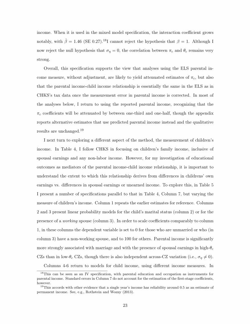
income. When it is used in the mixed model specification, the interaction coefficient grows

notably, with �̂ = 1.46 (SE 0.27).18I cannot reject the hypothesis that � = 1. Although I

now reject the null hypothesis that �⌘

= 0, the correlation between ⇡c

and ✓c

remains very

strong.

Overall, this specification supports the view that analyses using the ELS parental in-

come measure, without adjustment, are likely to yield attenuated estimates of ⇡c

, but also

that the parental income-child income relationship is essentially the same in the ELS as in

CHKS’s tax data once the measurement error in parental income is corrected. In most of

the analyses below, I return to using the reported parental income, recognizing that the

⇡

c

coefficients will be attenuated by between one-third and one-half, though the appendix

reports alternative estimates that use predicted parental income instead and the qualitative

results are unchanged.19

I next turn to exploring a different aspect of the method, the measurement of children’s

income. In Table 4, I follow CHKS in focusing on children’s family income, inclusive of

spousal earnings and any non-labor income. However, for my investigation of educational

outcomes as mediators of the parental income-child income relationship, it is important to

understand the extent to which this relationship derives from differences in childrens’ own

earnings vs. differences in spousal earnings or unearned income. To explore this, in Table 5

I present a number of specifications parallel to that in Table 4, Column 7, but varying the

measure of children’s income. Column 1 repeats the earlier estimates for reference. Columns

2 and 3 present linear probability models for the child’s marital status (column 2) or for the

presence of a working spouse (column 3). In order to scale coefficients comparably to column

1, in these columns the dependent variable is set to 0 for those who are unmarried or who (in

column 3) have a non-working spouse, and to 100 for others. Parental income is significantly

more strongly associated with marriage and with the presence of spousal earnings in high-✓c

CZs than in low-✓c

CZs, though there is also independent across-CZ variation (i.e., �⌘

6= 0).

Columns 4-6 return to models for child income, using different income measures. In18This can be seen as an IV specification, with parental education and occupation as instruments for

parental income. Standard errors in Column 7 do not account for the estimation of the first-stage coefficients,however.

19This accords with other evidence that a single year’s income has reliability around 0.5 as an estimate ofpermanent income. See, e.g., Rothstein and Wozny (2013).

23

column 4, only the child’s own earnings are included. For comparability, this is scaled in

terms of percentiles of the children’s family income distribution, just as in column 1. Thus,

a child with median earnings ($22,000 in the ELS sample) is assigned a percentile of 38,

as $22,000 is the 38th percentile of the family income distribution used in column 1. The

key interaction coefficient is about one-third smaller here than in column 1, suggesting that

a substantial portion of the across-CZ variation in income transmission operates through

channels other than the child’s own earnings. Column 2 adds non-labor income for the child’s

family, again scaled as a percentile of the child total family income distribution. This brings

the � coefficient up a bit, from 0.87 to 0.94, but it remains much less than the 1.46 in column

1. Evidently, spousal earnings are an important factor. This could reflect variation across

CZs in the relative likelihood that children from high- and low-income families have working

spouses, but it could also reflect differences in spousal earnings distributions conditional on

work, as would occur if CZs vary in the degree of assortative mating. Column 6 offers one

way to assess this. I compute the average earnings across the entire sample for working

spouses, by gender – $27,000 for women and $41,000 for men – and assign this to every

working spouse in the sample. The dependent variable in this column is constructed from

the sum of the child’s actual earnings, any non-labor income, and the imputed spousal

income, set to the average for those with working spouses and to zero for those without. As

before, this sum is converted to a percentile of the actual child family income distribution.

Here, the � coefficient is substantially increased, 1.53. Thus, the difference between results

for total family income and those based on childrens’ own earnings and non-labor income

is primarily due to differences (across parental income and across CZs) in the propensity to

have a working spouse, not in the spousal earnings distribution conditional on work.20

In the investigation below, I examine transmission of parental income into children’s

educational outcomes, then variation across CZs in the returns to education. Part of the

return to education may come through differences in the likelihood of having a working

spouse, and Table 5 indicates that there may be important differences across CZs in this

component of the return. I explore decompositions that account for this in Section 7.20Appendix Table A7 reports estimates of these specification separately by child gender. Interestingly, the

parental income main effects are quite different, but the � coefficients are quite similar for men and women.

24

5 Results: The transmission of parental income to children’s

human capital outcomes across CZs

This section contains the main results for the paper, examining the association across CZs

between CHKS’s parent income-child income transmission measure (✓c

) and measures from

the ELS, ECLS, and HSLS of the transmission from parental income to children’s human

capital outcomes (⇡c

). I begin by examining students’ test scores, then consider educational

attainment and the return to education.

5.1 Transmission to children’s test scores

Table 6 presents estimates of equation (14), using the ELS sample and the 12th grade

math score as the dependent variable. As in the earlier analysis of child incomes, I scale

test scores as percentiles in the ELS distribution; here, I return to the self-reported, noisy

parental income measure rather than predicted parental income used in Table 5. Column

1 indicates that on average, each percentile of parental income is associated with about

0.38 percentiles of children’s math scores. Columns 2 and 3 separate this into within- and

between-CZ components. The within-CZ coefficient is 0.35 or 0.34, but the between-CZ

coefficient is a fair amount larger. (As before, there is little distinction between between-CZ

and within-CZ, across-school variation, but the association between income and achievement

is only about half as strong within schools as between.) When I interact family income with

CZ-level income transmission, in column 4 (random effects) and column 5 (fixed effects),

the coefficients are 0.37 and 0.32, respectively. These are comparable in magnitude to the

parental income main effect. Recall that in the analysis of child income in Table 4, the

interaction coefficient was roughly quadruple the main effect.

Column 6 presents the mixed model. Here, the variance of the random component of

the income coefficient is quite large, accounting for 90% of the total variance of ⇡c

, and

I can decisively reject the null hypothesis of �⌘

= 0. The correlation between income-

test score transmission ⇡

c

and income-income transmission ✓

c

is only 0.32. This is hard

to reconcile with the hypothesis that test scores, or the knowledge and skill that they

represent, are a key mechanism determining intergenerational income transmission, since

25

there is evidently substantial variation in test score outcomes across CZs that does not

translate into corresponding variation in income transmission. I explore this argument more

formally below, in Section 7.

Table 7 presents mixed model estimates for each of the available test scores from the

ECLS, ELS, and HSLS. The � coefficients in column 2 are comparable in magnitude across

most of the specifications, though imprecisely estimated. The random component of the

parental income coefficient (�⌘

, in column 3) is meaningful in each specification, and column

6 indicates that the null hypothesis that �⌘

= 0 is rejected in all but one case. This random

component accounts for at least 80% of the overall variance of ⇡c

(column 5).

The pattern of results has several implications. First, there is some indication from the �

estimates (column 2) that the relative importance of parental income to student test scores

in high-income-transmission CZs grows between kindergarten and high school, consistent

with the hypothesis that differential access to school quality is a mechanism contributing

to differential income transmission. This is based largely on the ECLS kindergarten and

first grade results, however; there is much less evidence that coefficients rise after third

grade. Moreover, even the post-kindergarten growth in these coefficients is quite small.

Second, there is substantial heterogeneity across CZs in the transmission of parental income

to children’s test scores that is not associated with CZ-level income transmission (column

3), indicating that the institutions or other CZ characteristics that contribute to test score

transmission differ from those determining income transmission. Put somewhat differently,

there is only a weak correlation across CZs between income-income and income-test score

transmission (column 5), so different influences must be at work. Finally, results are quite

similar for the HSLS as for the ELS, suggesting that cohort differences are unable to explain

the weak relationship of income-income and income-test score transmission in the HSLS and

ECLS.

5.2 Transmission to children’s educational attainment

Table 8 presents results from specifications like those in Table 6, except this time using

measures of children’s eventual educational attainment – an indicator for any college, an

indicator for college graduation, and the number of years of education by age 26 – in place

26

of test scores. The first measure corresponds to CHKS’s analysis, while the other two

are more conventional measures. Not surprisingly, parental income is strongly related to

all three measures of children’s attainment. The interaction coefficient � is substantial and

statistically significant for college graduation and years of education, but is negative (though

insignificant) in the models for any college.

Even numbered columns present the mixed model specification. A likelihood ratio test

rejects the null hypothesis that the parental income random coefficient is zero (i.e., �⌘

= 0)

for the college attendance indicator but not for the other two outcomes. Even for these

outcomes, however, point estimates indicate that three-quarters of the across-CZ variation

in ⇡ is attributable to this random component rather than to CHKS’s income transmission

measure. (For the college attendance indicator, essentially all of the variation comes from the

random coefficient.) As in the earlier analysis of test scores, the evidence does not point to a

strong role for educational attainment as a mechanism driving variation in intergenerational

income transmission.

It is not clear how to account for the particularly weak results in columns 1-2, where

the dependent variable is an indicator for some college or more. This is the only attain-

ment construct that CHKS were able to measure in their tax data, and they found that

the transmission of parental income to children’s college enrollment (⇡c

in my notation)

was highly positively correlated (⇢ = 0.68) with income-to-income transmission. To ex-

plore this further, Appendix Table A1 repeats the analysis in Table 8, this time using the

CHKS parental income to college enrollment transmission measure in place of their income-

to-income transmission measure. With this switch, the � coefficient becomes positive and

statistically significant even for college enrollment. But the relationship remains quite weak,

with a coefficient far below the value (� = 1) we would expect under the null hypothesis that

income-to-college transmission is identical in the ELS as in the tax data. Moreover, each of

the other educational attainment measures is much more strongly related to CHKS’s college

transmission measure than is the simple college enrollment indicator. The most straight-

forward explanation seems to be that CHKS’s measure, which is based on the payment

of tuition at any college on a student’s behalf, is capturing a different phenomenon than

are traditional survey-based measures of college enrollment, based on respondents reporting

27

some educational attainment (including attendance at college without a degree) beyond high

school.21

Returning to the results for years of completed education, it is worth considering the

magnitude of the effects in Table 8 via a calculation like that in Section 2.1. In the ACS

sample described above, each additional year of education is associated with an additional

4.1 percentiles of children’s family income.22 Column 6 of Table 8 indicates that the standard

deviation across CZs of the parental income coefficient in a model for children’s educational

attainment (i.e., �⇡2) is 0.0026. Thus, a one standard deviation increase in ⇡2c would be

expected to generate an increase in ✓

c

of 0.0026*4.1 = 0.01 operating through educational

attainment. This is under one-sixth of a standard deviation of ✓c

. Moreover, this calculation

uses the total variation in the parental income coefficient (⇡2c), not just the part that is

collinear with income transmission (✓c

�). A one-standard deviation increase in the latter

is only 0.0013. This implies that differences in the transmission of parental education into

educational attainment can account for less than one-twelfth of the variation (in standard

deviation terms) across CZs in income transmission.

5.3 Robustness and additional results

The results above indicate that CZs in which the transmission of parental income to chil-

dren’s income is stronger tend not to be CZs in which there is strong transmission of parental

income to children’s test scores, either early or late in schooling careers. They are, on average,

CZs with stronger transmission of parental income into children’s educational attainment,

but even here the relationship is not very strong.

Appendix Table A2 explores the sensitivity of these results to the choice of an income

transmission measure. It presents mixed model specifications for three outcomes – child

income, 12th grade math scores, and years of education. In columns 1, 4, and 7, the21Note that the ELS sample reports a surprisingly high college enrollment rate – 84% of the sample reports

some postsecondary attendance or degree by age 26, where CHKS identify only 59% of their sample as havingattended college (using a somewhat different definition) by age 21. In ACS data, 58% have some collegeor more, with 17% having some college but no degree. A possible, partial explanation is that some of theELS respondents attend institutions not captured by the CHKS data. Fully 31% of the ELS sample reports“Some PS attendance, no PS credential,” the lowest category that I count as college enrollment.

22This rises to 5.9 when very low and very high values of attainment are trimmed. This would have littleeffect on the calculation here.

28

transmission measure is CHKS’s preferred measure for the 1980-82 birth cohorts, as in the

results above. In columns 2, 5, and 8, CHKS’s alternative measure for the 1983-85 birth

cohorts is used, while in columns 3, 6, and 9 the more plausibly causal measure from Chetty

and Hendren (2015) are used. Results are quite similar across measures: I find that all three

measures of ✓c

from tax data are strongly correlated with the ✓c

from the ELS data, weakly

correlated with ⇡2c when the educational outcome is the 12th grade math score, and more

strongly correlated when the outcome is educational attainment. The sole exception is the

educational attainment model based on the Chetty-Hendren transmission measure, where

the correlation is somewhat weaker but I cannot reject a perfect correlation.

CHKS document that their income transmission (relative mobility) measure is quite

strongly correlated with the fraction black in the CZ. Although they also find that an

alternative measure computed solely from zip codes with very few black residents is quite

similar, this nevertheless raises the possibility that race is an important confounding factor.

In Appendix Table A3, I add to the main mixed model specifications controls for the child’s

own race and gender, as well as interactions of race and gender with ✓

c

. This weakens the

income transmission and test score transmission results (such as they were), but has little

effect on the educational attainment results. There is absolutely no indication that failure

to account for race or gender in my earlier specifications has led me to understate the role

of educational achievement in income transmission.

Another concern, raised by Figure 2, above, is that my linear mixed model specification

misspecifies the relationship between parental income and children’s outcomes, particularly

test scores. To address this, I rescale parental income as p̃

ic

⌘ E [sic2|pic], where s

ic2 is

the child’s 12th grade test score. This ensures that E [sic2|p̃ic] is linear in p̃

ic

. (This could

also be accomplished by rescaling s

ic2, but as there is not a unique scaling that would

accomplish this I do not pursue it.) As Figure 2 indicates, the transformation from p

ic

to

p̃

ic

somewhat compresses the lower middle of the parental income distribution (around the

15th-20th percentiles) relative to the tails. Appendix Table A4 reproduces Table 6 using

the new parental income measure. The rescaling of course changes the scale of the parental

income coefficients, but does little to the relative magnitude of the interaction coefficient

� and does not alter the substantive conclusion that income transmission is not strongly

29

related to test score transmission. Appendix Table A5 uses predicted parental income (on

the original scaling), as in Table 4, column 7, for the main specifications. This does not

change the qualitative results for educational achievement or attainment.

Overall, the basic results on achievement, attainment, and income transmission appear

quite robust. They are suggestive that learning in school is not a key channel determining

the across-CZ variation in income transmission, but that access to higher education may be

more important.

One possibility not yet considered is that elementary and secondary schools do matter,

but that math and reading test scores do not capture their impacts. A growing literature

in recent years has documented the importance of non-cognitive skills as a component of

the learning process. Both the ECLS and the ELS contain batteries of questions aimed

at identifying children’s non-cognitive skills, and I use these to assess whether high-income-

transmission CZs tend to be CZs with large gaps in non-cognitive skills between children from

high- and low-income families. Appendix Table A6 presents specifications for non-cognitive

skill outcomes measured in the ELS 10th grade survey (Panel A) and the ECLS 5th grade

survey (Panel B), each converted to z-scores. Unfortunately, measures differ somewhat across

surveys. For about half of the measures, there is statistically significant variation across CZs

in the return to parental income (i.e., �⌘

6= 0), and the random component (⌘c

) generally

accounts for nearly all of the across-CZ variation. The � coefficient on the parental income

- CZ income transmission interaction is generally small and not statistically significant, and

frequently has the wrong sign. Overall, there is little indication that non-cognitive skills are

important mediators of income-to-income transmission. Panel C, however, tells a somewhat

different story. Like Panel B, this is based on the ECLS 5th grade wave, but in this case

the outcome variables derive from teachers’ reports of children’s non-cognitive skills rather

than from the children’s own responses. For these measures, there is evidence of parental

income-CZ income transmission interactions (i.e., of � 6= 0), which account for more of the

overall variation in ⇡

c

. It is not clear how to account for the discrepancy between these

results and those from the student self-reports in Panel B – even when the concepts overlap

(e.g., for externalizing problem behaviors), results are quite different. This may indicate that

high-transmission CZs tend to be CZs in which teachers are more biased in their assessments

30

of low-income children, but this is quite speculative.

6 Results: Returns to education

The above results have concerned the role of skills – achievement, attainment, and non-

cognitive skills – as mediators of the intergenerational transmission of income. In terms

of Figure 1, the results suggest that ⇡1c and ⇡2c are not primary mechanisms influencing

reduced-form transmission ✓

c

. This in turn implies that much of the variation in income

transmission must be due to direct effects of parental income on children’s income, controlling

for human capital (i.e., to ⇡3c), or to differences in the returns to human capital (i.e., in

�3c).

To investigate this, I turn to the ACS samples of 28-32 year olds surveyed in 2010-2012.

As before, I estimate mixed models, in this case allowing the return to education (specified

as percentiles of income per year of completed education) to vary both with the CHKS

income transmission measure and independently across CZs.

Results are presented in Table 9. Column 1 shows that each year of education is asso-

ciated with 4.1 percentiles of family income. Column 2 shows that this association is a bit

smaller within CZs, 3.9, and this is not much affected by the inclusion of random effects

(column 3) or fixed effects (column 5). Column 4 presents a simple interacted model with

CZ random effects but fixed coefficients. It indicates that the return to education is larger

in high-income-transmission CZs – the interaction coefficient is comparable in magnitude to

the income main effects (though recall that the transmission measure has standard deviation

0.065, so most CZs have returns to education within about 10% of the average shown in

columns 1-2). Column 6 presents the mixed model. There is also substantial, statistically

significant variation across CZs in the return to education conditional on the CHKS in-

come transmission measure, which accounts for less than one-quarter of the total across-CZ

variation in �3c. The overall variability in returns to education across CZs (i.e., in �3c) is

substantial, with a coefficient of variation of 16%.

31

7 Decomposing the variation in CZ-level income-income trans-

mission

The results thus far indicate that CZs with relatively strong intergenerational income trans-

mission tend to have stronger relationships between parental income and children’s educa-

tional attainment, only slightly stronger associations between parental income and children’s

test scores, and higher returns to education. Some preliminary calculations indicate that the

educational attainment relationships are not large enough to be primary channels in overall

income transmission, but I have not yet quantified the contributions of the test score or

returns to education effects. In this section, I explore decompositions of the across-CZ vari-

ation in the income-income relationship. I begin with three components: (a) children’s skill

accumulation by the end of school; (b) returns to skills; and (c) relationships between par-

ents’ incomes and the component of children’s incomes that is not attributable to observed

human capital. I then consider a second decomposition separates out a fourth component

corresponding to non-labor income and spousal earnings.

Suppose that z

ic

is a scalar measure of the human capital of child i from CZ c. We can

project children’s incomes onto this separately for each CZ:

y

ic

= z

ic

c

+ ⌫

ic

, (15)

where c

is the return to human capital in CZ c and ⌫

ic

is the income residual. Thus, the

relationship between children’s incomes and parents’ incomes in CZ c is:

dy

ic

dp

ic

=@z

ic

@p

ic

c

+@⌫

ic

@p

ic

. (16)

This is the definition of ✓c

, the income transmission measure. I label it ✓ELS

c

to indicate

that this relationship may differ somewhat based on the sample used to compute it. Now

consider how this varies with the CHKS transmission measure, ✓c

:

d✓

ELS

c

d✓

c

=d

2y

ic

dp

ic

d✓

c

=@

2z

ic

@p

ic

@✓

c

c

+@z

ic

@p

ic

@

c

@✓

c

+@

2⌫

ic

@p

ic

@✓

c

. (17)

32

The left side of this equation was estimated in column 6 of Table 4 as 0.65. (Recall that this

is attenuated due to measurement error in the ELS parental income variable.) The right side

has three components. The first term represents variation in human capital accumulation

gaps between high- and low-income families. This might occur, for example, if high-✓c

CZs

offer less equal school quality to children from different family backgrounds. The analysis

in Section 5 concerned this component. The second term in (17) reflects covariance of

the CZ-level return to skill with CZ-level income transmission, scaled by the overall average

difference in skill accumulation between high- and low-income families. For example, high-✓c

CZs may have fewer unions or just a more unequal income distribution, generating a higher

return to skill and thus producing better outcomes for children from high-income families.

This component was the focus of Section 6. The third term reflects differences in the

transmission of parental income to children’s incomes holding skills constant. This might be

large if high-✓c

CZs have more stratified labor (or marriage) markets or employment networks

that allow high-income parents to ensure good outcomes for their children regardless of the

children’s skills.

To implement this decomposition, I need a scalar index of human capital. I form this by

estimating a regression of children’s income percentiles on their educational attainment and

their 12th grade math scores, with CZ fixed effects, in the ELS sample. My human capital

index is the predicted value from this regression (neglecting the fixed effects). Note that

this method of forming z

ic

normalizes = 1 in the average CZ.

Column 1 of Table 10 repeats the basic random effects regression of children’s income

percentiles on parents’ income and its interaction with CZ-level income transmission, from

Table 4, Column 6. (The sample differs slightly from the one used earlier, as I exclude

observations with missing test scores or educational attainment.) The interaction coefficient

is 0.62.

In Column 2, I repeat the specification but use the child skill index z

ic

as the dependent

variable. Not surprisingly given the earlier results, the interaction terms, which represents

the first term of the decomposition (17), is small and not statistically significant. The point

estimate of 0.09 implies that skill accumulation accounts for only 15% (= 0.09/0.62) of the

differences in ELS income transmission between cities with low and high values of the CHKS

33

transmission measure.

Column 3 explores the role of returns to skill. Here, the dependent variable is the child’s

income percentile, but explanatory variables are the child’s skill index and its interaction

with the CZ-level income transmission. This interaction coefficient estimates @ c@✓c

; the second

term of the decomposition (17) can then be obtained by multiplying it by the average effect

of parental income on children’s skill, which by column 2 is 0.10. Thus, the second term is

0.21, indicating that differences in returns to skill account for 34% of the variation in income

transmission.

Column 4 returns to the specifications from columns 1 and 2, but here the dependent

variable is the residual from the column 3 regression (representing ⌫ic

in (15)). The inter-

action coefficient here is 0.31, indicating that half of the variation in income transmission is

attributable to differences in the transmission of parental income to child income controlling

for the child’s observable skills and for CZ-level differences in the returns to these skills.

The decomposition in Table 10 uses the child’s family income. A portion of the return to

skill component estimated in column 3 might reflect returns to skill on the marriage market

– higher skill children may be more likely to have working spouses in high-transmission CZs,

or might have spouses with higher earnings. Similarly, a portion of the residual component

in column 4 might reflect a relationship between parental income and spousal earnings or

family non-labor income conditional on the child’s skill accumulation. To explore this, I

decompose the child’s family income into his/her earnings and the remainder, reflecting

spousal earnings and non-labor income. As in Table 5, child earnings are scaled in terms

of percentiles of the child family income distribution, and the remainder is measured as the

increase in percentiles when the other components of family income are included.

Results are in Table 11. Columns 1-4 are the same as in Table 10, though now only

the child’s own earnings are permitted to contribute to the returns to skill (column 3) or

the earnings residual (column 4). The contribution of returns to skill is halved relative to

Table 10, and the contribution of residual income transmission by about one-third. Column

5 presents results for the non-earnings component of family income. This accounts for about

one-third of the variation across CZs in parent income - child family income transmission.

Based on Table 5, this primarily reflects differences in the relative propensity of children from

34

high- and low-income families to have working spouses, rather than differences in non-labor

income or in spousal earnings conditional on work.

A natural question is whether this decomposition differs by gender. Interestingly, when

I implement the decomposition in Table 11 separately for boys and girls, in Appendix Table

A8, the non-earnings component (column 5) is quite similar for both. The primary difference

between the two is that the skill accumulation (column 2) and return to skill (column 3)

components are much smaller for girls than for boys, while the earnings residual component

(column 4) is much larger. Even for boys, however, skill accumulation accounts for less than

one-fifth of the variation in income transmission, and returns to skill for one-third, with over

half operating through earnings residuals and spousal and non-labor income.

8 Conclusion

Chetty et al.’s (2014) pathbreaking work showed that there is dramatic variation in inter-

generational income mobility across geographic areas within the United States. This raises

the intriguing possibility that we can identify policies that account for this variation and,

by exporting these policies from high- to low-mobility areas, move closer to equality of

opportunity.

CHKS presented suggestive correlations that indicated that school quality might be an

important contributing factor. This paper has investigated this suggestion further, by asking

whether high- and low-income children’s academic outcomes are more equal in areas where

their adult economic outcomes are more equal – that is, in areas with more intergenerational

mobility. I find that there is statistically significant variation across commuting zones in the

gradients of educational attainment, academic achievement, and non-cognitive skills with

respect to parental income. Intergenerational income transmission is reasonably strongly

correlated with the educational attainment gradient and with the labor market return to

education, but does not covary strongly with either academic achievement or non-cognitive

skill gradients (with the exception of gradients computed from teacher reports of children’s

non-cognitive skills).

I find that only about one-tenth of the across-CZ variation in intergenerational income

35

mobility is attributable to differences in children’s earnings deriving from differences in

skill accumulation. A slightly larger share is attributable to differences in the labor market

returns to children’s skills. About one-third is attributable to differences in the labor market

return to parental income holding skills (and the returns to skills) constant. The remaining,

largest portion derives from differences in spousal and non-labor income, primarily reflecting

differences in the likelihood of having a working spouse.

Although this evidence is observational rather than causal, it strongly suggests that

differences in elementary and secondary school quality are not an important determinant

of variation in income mobility. (This is not to say that school quality is not important

for other reasons, of course, or even that it does not contribute to overall mobility in a

way that is roughly constant across CZs.) There appears to be more of a role for access

to higher education in driving economic mobility, though even here the contribution is

not large relative to the overall variation. Further investigation into the determinants of

local intergenerational mobility should focus on differences in the returns to education, in

the returns to family income conditional on children’s human capital, and in the relative

propensity of children from high- and low-income families to have working spouses. Plausible

factors driving the former might include institutions determining local income inequality,

such as state income taxation and union density. The second, reflecting direct effects of

parental income on children’s earnings conditional on children’s human capital, might reflect

variation in the importance of labor market networks or in spatial or social stratification

of the labor market. The third seems to reflect differences in the likelihood of marriage

rather than variation in assortative mating; insofar as this reflects differences across CZs

in the likelihood that romantic partners will be formally married rather than differences

in the likelihood of partnership, it may not represent meaningful variation in equality of

opportunity.

36

References

Aaronson, D. and B. Mazumder (2008). Intergenerational economic mobility in the UnitedStates, 1940 to 2000. Journal of Human Resources 43 (1), 139–172.

Bond, T. N. and K. Lang (2013). The evolution of the black-white test score gap in gradesK–3: The fragility of results. Review of Economics and Statistics 95 (5), 1468–1479.

Bradbury, B., M. Corak, J. Waldfogel, and E. Washbrook (2015). Too many children leftbehind: The US achievement gap in comparative perspective. Russell Sage Foundation.

Carneiro, P. and J. J. Heckman (2003). Human capital policy. In B. M. Friedman (Ed.),Inequality in America: What Role for Human Capital Policies? MIT Press.

Chetty, R., D. Grusky, M. Hell, N. Hendren, R. Manduca, and J. Narang (2016). The fadingAmerican dream: Trends in absolute income mobility since 1940. working paper 22910,National Bureau of Economic Research, December.

Chetty, R. and N. Hendren (2015). The impacts of neighborhoods on intergenerationalmobility: Childhood exposure effects and county-level estimates. Unpublished manuscript,Harvard University and NBER.

Chetty, R., N. Hendren, P. Kline, and E. Saez (2014). Where is the land of opportunity?The geography of intergenerational mobility in the United States. The Quarterly Journalof Economics 129 (4), 1553–1623.

Chetty, R., N. Hendren, P. Kline, E. Saez, and N. Turner (2014). Is the United Statesstill a land of opportunity? Recent trends in intergenerational mobility. The AmericanEconomic Review 104 (5), 141–147.

Cunha, F. and J. Heckman (2007). The economics of human development: The technologyof skill formation. The American Economic Review 97 (2), 31–47.

Cunha, F. and J. J. Heckman (2008). Formulating, identifying and estimating the technologyof cognitive and noncognitive skill formation. Journal of Human Resources 43 (4), 738–782.

Cunha, F., J. J. Heckman, and S. M. Schennach (2010). Estimating the technology ofcognitive and noncognitive skill formation. Econometrica 78 (3), 883–931.

Gelman, A. and J. Hill (2006). Data analysis using regression and multilevel/hierarchicalmodels. Cambridge University Press.

Jacob, B. and J. Rothstein (2016, Summer). The measurement of student ability in modernassessment systems. Journal of Economic Perspectives 30 (3), 85–108.

Kearney, M. S. and P. B. Levine (2014). Income inequality and early nonmarital childbearing.Journal of Human Resources 49 (1), 1–31.

Kearney, M. S. and P. B. Levine (2016). Income inequality, social mobility, and the decisionto drop out of high school. Brookings Papers on Economic Activity , 367.

37

Mazumder, B. (2005). Fortunate sons: New estimates of intergenerational mobility in theUnited States using Social Security earnings data. Review of Economics and Statis-tics 87 (2), 235–255.

National Center for Education Statistics (undated). ELS:2012 student codebook. Technicalreport. Retrieved from http://nces.ed.gov/pubs2014/ELS2012_codebook_Student1.

pdf on April 6, 2017.

Nielsen, E. R. (2015). Achievement gap estimates and deviations from cardinal comparabil-ity. Finance and Economics Discussion Series 2015-04, Board of Governors of the FederalReserve System.

Reardon, S. F. (2011). The widening academic achievement gap between the rich and thepoor: New evidence and possible explanations. In G. J. Duncan and R. J. Murnane (Eds.),Whither Opportunity? Rising Inequality and the Uncertain Life Chances of Low-IncomeChildren, Chapter 5, pp. 91–116. New York: Russell Sage Foundation Press.

Rothstein, J. (2004). College performance predictions and the SAT. Journal of Economet-rics 121 (1), 297–317.

Rothstein, J. and N. Wozny (2013). Permanent income and the black-white test score gap.Journal of Human Resources 48 (3), 510–544.

Tourangeau, K., C. Nord, T. Lê, J. M. Pollack, and S. Atkins-Burnett (2006). Early Child-hood Longitudinal Study, Kindergarten class of 1998-99 (ECLS-K), combined user’s man-ual for the ECLS-K fifth-grade data files and electronic codebooks. Technical ReportNCES 2006-032, National Center for Education Statistics, U.S. Department of Educa-tion, Washington D.C.

38

Figure 1: Academic achievement as mediator of the effect of parental income on children's income

Parental income(pic)

Early child achievementsic1=κ1c+picπ1c+u1ic

Later child achievementsic2=κ2c+sic1λ2c+picπ2c+u2ic

Child incomeyic=κ3c+sic2λ3c+picπ3c+εic

π1c

π2c

π3c

λ2c

λ3c

Figure 2. Average ELS outcomes by parent income

B. Child earnings percentileA. Child family income percentile

C. 12th grade math score percentile D. Years of education at age 26

Note : Each point represents a response to the ELS parental income question, converted to a percentile (and assigned to the midpoint of the relevant range). The small "x" represents the average outcome for the 0.2% of observations reporting zero parental income. Child family income, earnings, and 12th grade math scores are each measured as percentiles of the relevant national distribution.

3540

4550

5560

Chi

ld fa

mily

inco

me

perc

entil

e

0 20 40 60 80 100Parent income percentile

13.5

1414

.515

15.5

Year

s of

edu

catio

n at

26

0 20 40 60 80 100Parent income percentile

4045

5055

60C

hild

ear

ning

s pe

rcen

tile

0 20 40 60 80 100Parent income percentile

3040

5060

7012

th g

rade

mat

h sc

ore

perc

entil

e

0 20 40 60 80 100Parent income percentile

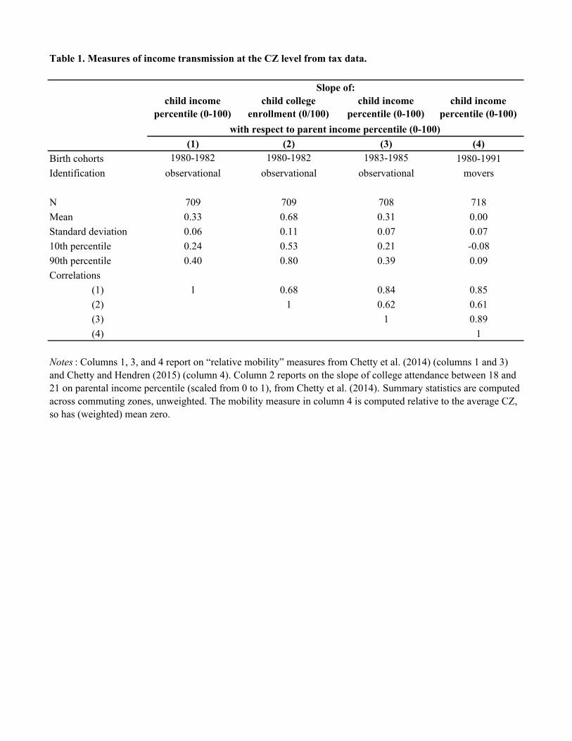
Table 1. Measures of income transmission at the CZ level from tax data.

child income percentile (0-100)

child college enrollment (0/100)

child income percentile (0-100)

child income percentile (0-100)

(1) (2) (3) (4)Birth cohorts 1980-1982 1980-1982 1983-1985 1980-1991Identification observational observational observational movers

N 709 709 708 718Mean 0.33 0.68 0.31 0.00Standard deviation 0.06 0.11 0.07 0.0710th percentile 0.24 0.53 0.21 -0.0890th percentile 0.40 0.80 0.39 0.09Correlations

(1) 1 0.68 0.84 0.85(2) 1 0.62 0.61(3) 1 0.89(4) 1

with respect to parent income percentile (0-100)

Slope of:

Notes : Columns 1, 3, and 4 report on “relative mobility” measures from Chetty et al. (2014) (columns 1 and 3) and Chetty and Hendren (2015) (column 4). Column 2 reports on the slope of college attendance between 18 and 21 on parental income percentile (scaled from 0 to 1), from Chetty et al. (2014). Summary statistics are computed across commuting zones, unweighted. The mobility measure in column 4 is computed relative to the average CZ, so has (weighted) mean zero.

Table 2. Summary statistics for NCES samples

Early Childhood

Longitudinal Study (ECLS)

High School Longitudinal Study (HSLS)

Educational Longitudinal Study (ELS)

(1) (2) (3)Birth year 1992-1993 1994-1995 1985-1986N 19,940 21,440 15,240# of CZs 365 295 312Demographics

Female 0.48 0.50 0.50Black 0.18 0.17 0.14Hispanic 0.19 0.22 0.16Asian 0.03 0.03 0.04Other non-white 0.02 0.08 0.05

Parent income 51,789 77,730 61,417(47,419) (128,331) (50,312)

Parent income percentile 48.9 49.6 50.0(29.0) (29.0) (28.5)

Test scores available for grades K,1,2,3,5,8 9,11 10,12Post-high school outcomes (from 2012 follow-up survey)

Any college 0.84College completion 0.33Years of education 14.0

(1.8)Income at age 26 36,095

(35,238)Income percentile at age 26 50.0

(28.9)

Note : Sample sizes and demographics are computed for the base-year sample for each survey, and use sampling weights. Sample sizes are rounded to the nearest 10. Standard deviations in parentheses.

Table 3. Cross-sectional regressions of child outcomes on parental income

Number of observations

Number of observations

(1) (2) (3) (4) (5) (6)CZ FEs N Y N YECLS-K

K (spring) 0.41 0.40 19,190 0.37 0.36 18,500(0.01) (0.01) (0.01) (0.01)

G1 (spring) 0.40 0.41 16,370 0.38 0.37 16,080(0.01) (0.01) (0.01) (0.01)

G3 0.44 0.42 14,180 0.45 0.43 14,090(0.01) (0.01) (0.01) (0.01)

G5 0.45 0.43 11,140 0.45 0.43 11,130(0.02) (0.02) (0.02) (0.02)

G8 0.44 0.42 9,210 0.46 0.44 9,150(0.02) (0.02) (0.02) (0.02)

HSLSG9 0.36 0.32 20,170

(0.01) (0.01)G11 0.35 0.31 20,460

(0.01) (0.01)ELS

G10 0.37 0.34 15,240 0.35 0.32 15,240(0.01) (0.01) (0.01) (0.01)

G12 0.38 0.35 13,650(0.01) (0.01)

Any college (*100) 0.26 0.24 13,250(0.01) (0.01)

College completion (*100) 0.49 0.45 13,250(0.02) (0.02)

Years of education (*100) 2.04 1.87 13,250(0.07) (0.07)

Income at 26 0.18 0.16 11,510(0.01) (0.01)

Math Reading

Notes : Each entry represents the coefficient from a separate weighted least squares regression of the child's outcome on family income. Columns 2 and 5 add fixed effects for commuting zones. Parental incomes, test scores, and child incomes are measured in percentile units, scaled 0-100. Any college and college completion are binary, but scaled as 0/100 for readability; years of education is multiplied by 100 for the same reason. Sample sizes in columns 3 and 6 are rounded to the nearest 10.

Table 4. Parent income - child income relationships in the ELS

(1) (2) (3) (4) (5) (6) (7)Parental income 0.18

(0.01)Parental income - CZ mean 0.16 0.17 0.17 0.16 0.17 0.24

(0.01) (0.01) (0.01) (0.01) (0.01) (0.02)CZ mean parental income 0.32 0.35 0.35 0.35 0.48

(0.04) (0.04) (0.04) (0.04) (0.05)(Parental income - CZ mean) * 0.63 0.64 0.65 1.46

CZ income transmission (0.16) (0.20) (0.16) (0.27)SD of parental income random 0.01 0.10

coefficient (K) (0.02) (0.03)Parental income measure Actual Actual Actual Actual Actual Actual Pred.CZ controls None None RE RE FE RE RESD of total parental income coefficient (S) 0.038 0.127Share of variance attributable to CZ income transmission 95% 42%p-value, share of variance = 100% (LR test) 0.86 0.01Corr(tax data income transmission, ELS S) 0.97 0.65

Notes: Dependent variable in each column is the child's family income at age 26, in percentile units (0-100). Parental income is also measured in percentiles (0-100). CZ income transmission is the observational relative mobility measure for the 1980-82 birth cohorts from Chetty et al. (2014), demeaned across CZs. Column 7 uses the predicted parental income percentile in place of the reported value, for both main effects and interactions. Parental income is predicted based on a (weighted) regression of the reported income percentile on indicators for mother’s years of education, mother’s occupation, and father’s years of education and occupation (interacted with an indicator for father presence). Specifications labeled “RE” and “FE” include CZ random effects and fixed effects, respectively; columns 4, 6, and 7 also include main effects for CZ income transmission. Specifications in columns 1, 2, and 5 are weighted using ELS sampling weights; others are unweighted. Standard errors are clustered at the CZ level. p-values in columns 6-7 are for likelihood ratio tests of the mixed models against random effects models with fixed coefficients (as in column 4). Number of observations (rounded to the nearest 10) = 11,510 (10,950 in column 7).

Table 5. Parent income - child income relationships in the ELS

Child family income

Marital status (0/100)

Working spouse (0/100)

Child earnings

Child earnings + nonlabor income

Child earnings + non-labor income +

imputed spousal earnings

(1) (2) (3) (4) (5) (6)Parental income - CZ mean 0.24 -0.01 0.02 0.23 0.27 0.22

(0.02) (0.03) (0.03) (0.02) (0.02) (0.02)CZ mean parental income 0.48 -0.01 0.12 0.43 0.48 0.42

(0.05) (0.12) (0.11) (0.05) (0.05) (0.05)(Parental income - CZ mean) * 1.46 1.17 1.14 0.87 0.94 1.53 CZ income transmission (0.27) (0.47) (0.50) (0.26) (0.24) (0.27)

0.10 0.13 0.15 0.07 0.06 0.10(0.03) (0.05) (0.05) (0.04) (0.03) (0.03)

SD of total parental income coefficient (S) 0.127 0.150 0.159 0.083 0.080 0.132Share of variance attributable to CZ income transmission 42% 19% 16% 35% 44% 43%p-value, share of variance = 100% (LR test) 0.01 0.10 0.05 0.45 0.61 <0.01Corr(tax data income transmission, ELS S) 0.65 0.44 0.40 0.59 0.66 0.66

Notes: All specifications are unweighted linear regressions with fixed coefficients, a CZ random effect, a main effect for CZ income transmission, and a random coefficient on parental income that varies at the CZ level, as in Table 4, column 7. Only the dependent variable changes across columns. In columns 1, 4, 5, and 6, dependent variable is a measure of child income, with varying definitions, scaled as percentiles of the child total family income distribution; in columns 2 and 3, dependent variable is an indicator for being married or for having a working spouse, multiplied by 100. In all columns, parental income is the predicted percentile, described in notes to Table 4. CZ income transmission is the observational relative mobility measure for the 1980-82 birth cohorts from Chetty et al. (2014), demeaned across CZs. Standard errors are clustered at the CZ level. p-values are for likelihood ratio tests of the mixed models against random effects models with fixed coefficients (as in Table 4, column 4). Number of observations (rounded to the nearest 10) = 10,940.

SD of parental income random coefficient (K)

Table 6. Parental income and children's 12th grade math achievement in the ELS

(1) (2) (3) (4) (5) (6)Parental income 0.38

(0.01)Parental income - CZ mean 0.35 0.34 0.34 0.35 0.33

(0.01) (0.01) (0.01) (0.01) (0.01)CZ mean parental income 0.69 0.71 0.71 0.71

(0.04) (0.04) (0.04) (0.04)(Parental income - CZ mean) * 0.37 0.32 0.41 CZ income transmission (0.15) (0.21) (0.17)SD of parental income random coefficient (K) 0.07

(0.02)CZ controls None None RE RE FE RESD of total parental income coefficient (S) 0.07Share of variance attributable to CZ income transmission 10%p-value, share of variance = 100% (LR test) <0.01Corr(tax data income transmission, ELS S) 0.32

Notes : Dependent variable in each column is the 12th grade math score, in national percentile units (0-100). Parental income is also measured in percentiles (0-100). CZ income transmission is the observational relative mobility measure for the 1980-82 birth cohorts from Chetty et al. (2014), demeaned across CZs. Specifications labeled “RE” and “FE” include CZ random effects and fixed effects, respectively; columns 4 and 6 also include main effects for CZ income transmission. Specifications in columns 1, 2, and 5 are weighted using ELS sampling weights; others are unweighted. Standard errors are clustered at the CZ level. p-value in column 6 is for a likelihood ratio test of the mixed model against the random effects model with fixed coefficients in column 4. Number of observations (rounded to the nearest 10) = 13,650.

Parental income - CZ mean

Parental income * CZ

income transmission

SD of parental income random coefficient (K)

SD of total parental income

coefficient (S)

Explained share of variance

p-value, share of

variance = 100%

(1) (2) (3) (4) (5) (6)Panel A: Math scoresECLS K (spring) 0.38 0.16 0.08 0.08 0.01 <0.01

(0.01) (0.23) (0.01)ECLS G1 (spring) 0.38 0.23 0.06 0.06 0.05 <0.01

(0.01) (0.22) (0.01)ECLS G3 0.40 0.41 0.06 0.07 0.14 <0.01

(0.01) (0.21) (0.02)ECLS G5 0.39 0.50 0.06 0.07 0.19 <0.01

(0.01) (0.21) (0.01)ECLS G8 0.39 0.34 0.04 0.05 0.17 0.17

(0.01) (0.21) (0.02)HSLS G9 0.30 0.30 0.05 0.05 0.10 0.02

(0.01) (0.17) (0.01)HSLS G11 0.28 0.59 0.07 0.07 0.18 <0.01

(0.01) (0.17) (0.01)ELS G10 0.31 0.36 0.06 0.07 0.09 <0.01

(0.01) (0.17) (0.01)ELS G12 0.33 0.41 0.07 0.07 0.10 <0.01

(0.01) (0.17) (0.02)Panel B: Reading scoresECLS K (spring) 0.35 0.33 0.08 0.08 0.06 <0.01

(0.01) (0.26) (0.01)ECLS G1 (spring) 0.35 0.07 0.06 0.06 0.01 <0.01

(0.01) (0.24) (0.01)ECLS G3 0.42 0.13 0.08 0.08 0.01 <0.01

(0.01) (0.23) (0.01)ECLS G5 0.39 0.32 0.09 0.09 0.04 <0.01

(0.01) (0.26) (0.01)ECLS G8 0.41 0.24 0.07 0.07 0.04 <0.01

(0.01) (0.22) (0.02)ELS G10 0.30 0.24 0.08 0.08 0.03 <0.01

(0.01) (0.18) (0.01)

Table 7. Variation in parental income - child achievement relationships across grades, cohorts, and subjects

Notes : Each row presents a single mixed model regression pertaining to a different test score (for a given sample, grade, and subject), each scaled as national percentile units (0-100). Specifications are as in Table 6, column 6; see that table for details. Number of observations (rounded to the nearest 10) varies from 9,200 (ECLS-K, 8th grade math) to 20,430 (HSLS, 11th grade math).

Table 8. Parental income - children's educational attainment relationships in the ELS

(1) (2) (3) (4) (5) (6)Parental income - CZ mean 0.22 0.24 0.45 0.45 1.85 1.86

(0.01) (0.01) (0.02) (0.02) (0.06) (0.06)CZ mean parental income 0.50 0.49 1.01 1.01 4.12 4.14

(0.05) (0.05) (0.06) (0.06) (0.26) (0.26)(Parental income - CZ mean) * -0.11 -0.19 0.64 0.74 2.28 2.39 CZ income transmission (0.20) (0.21) (0.30) (0.29) (1.12) (1.09)SD of parental income random coefficient (K) 0.10 0.08 0.23

(0.02) (0.03) (0.13)SD of total parental income coefficient (S) 0.10 0.09 0.26Share of variance attributable to CZ income transmission 1% 23% 26%p-value, share of variance = 100% (LR test) <0.01 0.15 0.36Corr(tax data income transmission, ELS S) -0.10 0.48 0.51

College graduation

(0/100)

Years of education at 26

(*100)

Notes : Specifications are as in Table 6, columns 4 (odd numbered columns here) and 6 (even numbered columns). See notes to that table for details. Dependent variables in columns 1-4 are scaled as 0 for failures and 100 for successes; in columns 5-6, dependent variable is years of education multiplied by 100. Standard errors are clustered at the CZ level. Number of observations (rounded to the nearest 10) = 13,250.

Any college (0/100)

Table 9. Returns to education in American Community Survey (ACS) data

(1) (2) (3) (4) (5) (6)Years of education 4.12

(0.07)Years of education - CZ mean 3.94 3.99 4.03 4.02 3.84

(0.06) (0.05) (0.04) (0.04) (0.04)CZ mean education 9.36 5.59 5.54 5.23

(0.87) (0.28) (0.27) (0.27)(Education - CZ mean) * 4.92 4.91 5.12 CZ income transmission (0.66) (0.68) (0.77)SD of education random coefficient (K) 0.55

(0.04)CZ controls None None RE RE FE RESD of total education coefficient (S) 0.62Share of variance attributable to CZ income transmission 22%p-value, share of variance = 100% (LR test) <0.01Corr(tax data income transmission, ELS O) 0.47

Notes : Sample consists of individuals born 1980-1982 in the ACS 2010-2012 one-year public use microdata samples (N=253,852). Respondents are assigned to their CZ of current residence. Dependent variable in each specification is the child's family income percentile (0-100). Years of education is naturally coded. CZ income transmission is the observational measure for the 1980-82 birth cohorts from Chetty et al. (2014), demeaned across CZs. Specifications labeled “RE” and “FE” include CZ random effects and fixed effects, respectively; columns 4 and 6 also include main effects for CZ income transmission. Specifications in columns 1 and 2 are weighted using ACS sampling weights; others are unweighted. Standard errors are clustered at the CZ level. p-value in column 6 is for a likelihood ratio test of the mixed model against the random effects model with fixed coefficients in column 4.

Table 10. Decomposition of the variation in intergenerational income transmission

Mechanism Total transmission

Skills Return to skills

Residual

Dependent variableChild income

Child skill index

Child income

Child income residual

(1) (2) (3) (4)Parental income - CZ mean 0.16 0.10 0.07

(0.01) (0.00) (0.01)CZ mean parental income 0.33 0.21 0.05

(0.04) (0.01) (0.02)CZ income transmission 1.57 -3.79 -0.62 -2.85

(7.55) (1.90) (7.54) (3.57)(Parental income - CZ mean) * 0.62 0.09 0.31

CZ income transmission (0.17) (0.05) (0.15)Skill index - CZ mean 0.98

(0.04)CZ mean skill index 1.25

(0.13)(Skill index - CZ mean) * 2.24

CZ income transmission (0.59)0.10

Scaled component 0.09 0.21 0.31100% 15% 34% 50%

d skills / d parental income (scale factor)

Share of total

Notes : Sample consists of 9,980 observations (rounded to the nearest 10) from the ELS sample with complete information on 12th grade math scores, educational attainment and family income at age 25, and parental income. All specifications are unweighted random effects models with fixed coefficients, main effects for CZ income transmission (demeaned across CZs), CZ random effects, and standard errors clustered at the CZ level, as in Table 4, column 4. Child income in column 1 is child family income, including own and spousal earnings plus non-labor income, scaled as national percentiles (0-100). The skill index in columns 2 and 3 is the predicted value from a CZ fixed effects regression of children's family income percentiles on 12th grade math scores and indicators for years of schooling completed, estimated using third follow-up (2012) sampling weights. The child income residual is the residual from the regression in column 3. Parental income is measured in percentiles (0-100).

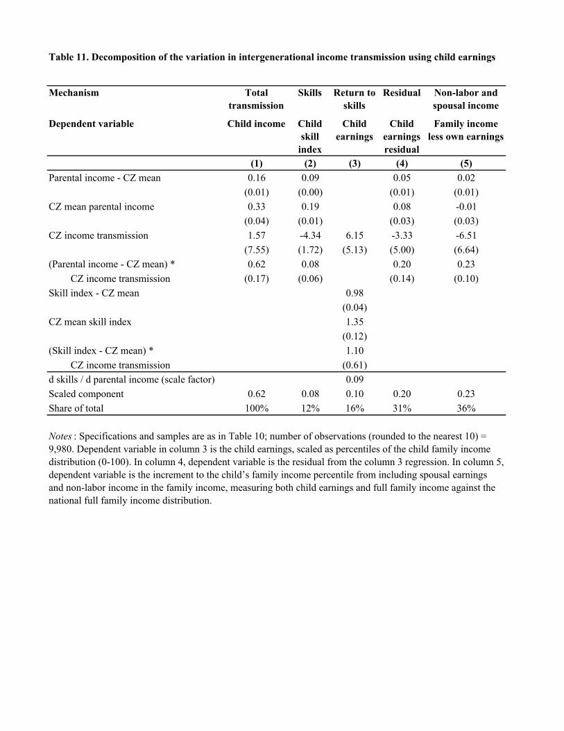
Mechanism Total transmission

Skills Return to skills

Residual Non-labor and spousal income

Dependent variable Child income Child skill

index

Child earnings

Child earnings residual

Family income less own earnings

(1) (2) (3) (4) (5)Parental income - CZ mean 0.16 0.09 0.05 0.02

(0.01) (0.00) (0.01) (0.01)CZ mean parental income 0.33 0.19 0.08 -0.01

(0.04) (0.01) (0.03) (0.03)CZ income transmission 1.57 -4.34 6.15 -3.33 -6.51

(7.55) (1.72) (5.13) (5.00) (6.64)(Parental income - CZ mean) * 0.62 0.08 0.20 0.23

CZ income transmission (0.17) (0.06) (0.14) (0.10)Skill index - CZ mean 0.98

(0.04)CZ mean skill index 1.35

(0.12)(Skill index - CZ mean) * 1.10

CZ income transmission (0.61)d skills / d parental income (scale factor) 0.09Scaled component 0.62 0.08 0.10 0.20 0.23

100% 12% 16% 31% 36%Share of total

Notes : Specifications and samples are as in Table 10; number of observations (rounded to the nearest 10) = 9,980. Dependent variable in column 3 is the child earnings, scaled as percentiles of the child family income distribution (0-100). In column 4, dependent variable is the residual from the column 3 regression. In column 5, dependent variable is the increment to the child’s family income percentile from including spousal earnings and non-labor income in the family income, measuring both child earnings and full family income against the national full family income distribution.

Table 11. Decomposition of the variation in intergenerational income transmission using child earnings

Appendix A: Additional results

Appendix Tables A1-A8 present additional specifications and results not included in themain tables.

Table A1 presents results for the three ELS educational attainment measures consideredin Table 8, but replaces the income transmission (relative mobility) measure with CHKS’seducation mobility measure, defined as the slope of college enrollment at age 18-21 (scaled as0 for non-enrollment and 100 for enrollment) with respect to parental income (in percentiles,0-100).

Table A2 explores two alternative income transmission (relative mobility) measures. Oneis the alternative measure computed by CHKS for the younger, 1983-5 birth cohorts, withadult incomes measured at younger ages. The second is the measure constructed by Chettyand Hendren (2015) based on families that move from one CZ to another. Three dependentvariables are considered: Children’s adult family income (in percentiles, 0-100), children’s12th grade math scores (also in percentiles), and the child’s years of completed educationas of age 26 (multiplied by 100).

Table A3 considers the same three outcomes and the baseline CHKS mobility measurefor the 1980-2 cohorts, but adds to the base specification indicators for the child’s raceand gender and, in columns 3, 6, and 9, interactions of these with the income transmissionmeasure.

Table A4 explores the potential impact of nonlinearity in the child test score - parentalincome relationship. I rescale parental income by replacing each value with the sampleaverage test score among all observations with the same reported parental income. Thisensures that the relationship is perfectly linear, on average.

Table A5 reports my main mixed specifications for the three primary outcomes, compar-ing those that use reported parental income with those that use predicted parental incomebased on maternal education and occupation, the presence of the father, and the paternaleducation and occupation (when present).

Table A6 reports estimates for a variety of non-cognitive measures from the ELS andECLS. These measures are described in Appendix B.

Table A7 reports specifications from Table 5, separately for male and female children.Table A8 repeats this exercise for Table 11.

Appendix B: Non-cognitive skill measures

Appendix Table A6 presents results for several different measures of non-cognitive skillsfrom the ELS 10th grade survey and the ECLS 5th grade student and teacher surveys. Idescribe these measures here.

ELS 10th grade survey. Each of the measures used is created by principal factor analysisfrom student responses to questions of the form “How often do these things apply toyou?”, with response options “almost never,” “sometimes,” “often,” and “almost always.”Quotations are from National Center for Education Statistics (undated).

i

Instrumental motivation. Intended to capture “motivation to perform well academ-ically in order to satisfy external goals like future job opportunities or financialsecurity.” Based on three responses about whether the student studies in orderto achieve long-run success.

General effort and persistence. Based on five questions characterizing effort putinto studying.

General control beliefs. Intended to capture “expectations of success in academiclearning.” Based on four responses characterizing the student’s self-perceivedability to achieve desired academic outcomes.

Self efficacy, math. Based on five responses characterizing the student’s self-perceivedability to succeed in math classes and his/her views about the importance of in-nate ability in math.

Self efficacy, reading. Based on five responses characterizing the student’s self-perceivedability to succeed in reading classes.

ECLS 5th grade student survey. Students rated 42 statements about their perceptionsof themselves as “not at all true,” “a little bit true,” “mostly true,” and “very true.”These were averaged into several scales. Quotations are from Tourangeau et al. (2006).

Perceived interest / competence in reading. Eight statements concerning “read-ing grades, the difficulty of reading work, and [the student’s] interest in andenjoyment of reading.”

Perceived interest / competence in math. Eight statements concerning “math-ematics grades, the difficulty of mathematics work, and [the student’s] interest inand enjoyment of mathematics.”

Perceived interest / competence in all school subjects. Six statements concern-ing “how well [the student] do[es] in ’all school subjects’ and [the student’s] en-joyment of ’all school subjects.” ’

Perceived interest / competence in peer relations. Six statements concerning“how easily [the student] make[s] friends and get[s] along with children as well astheir perception of their popularity.”

Externalizing problem behaviors. Six statements concerning “externalizing prob-lem behaviors such as fighting and arguing ’with other kids,’ talking and disturb-ing others, and problems with distractibility.”

Internalizing problem behaviors. Eight statements concerning “internalizing prob-lem behaviors such as feeling ’sad a lot of the time,’ feeling lonely, feeling ashamedof mistakes, feeling frustrated, and worrying about school and friendships."

ECLS 5th grade teacher survey. Teachers rated 26 statements about how often studentsexhibited certain social skills and behaviors as “never,” “sometimes,” “often,” and “very

ii

often.” These were averaged into several scales. Quotations are from Tourangeau et al.(2006).

Approaches to learning. “Measures behaviors that affect the ease with which chil-dren can benefit from the learning environment.” Based on seven items relatingto “the child’s attentiveness, tax persistence, eagerness to learn, learning inde-pendence flexibility, [] organization ... [and] child follows classroom rules.”

Self control. “Four items that indicate the child’s ability to control behavior by re-specting the property rights of others, controlling temper, accepting peer ideasfor group activities, and responding appropriately to pressure from peers.”

Interpersonal skills. “Five items that rate the child’s skill in forming and main-taining friendships; getting along with people who are different; comforting orhelping other children; expressing feelings, ideas, and opinions in positive ways;and showing sensitivity to the feelings of others.”

Peer relations. This is a combination of the self-control and interpersonal scales.Externalizing problem behaviors. This scale “includes acting out behaviors”: six

items “rate the frequency with which a child argues, fights, gets angry, acts im-pulsively, [] disturbs ongoing activities ... [and] talks during quiet study time.”

Internalizing problem behaviors. Four items ask about “the apparent presence ofanxiety, loneliness, low self-esteem, and sadness.”

For all of the non-cognitive items, I reverse-code so that higher values are better, thenconvert to percentiles. To form overall indices from each survey, I convert each listed scaleto a z-score, average them, then convert the average to percentiles.

iii

(1) (2) (3) (4) (5) (6)

Parental income - CZ mean 0.22 0.23 0.46 0.45 1.86 1.85(0.01) (0.01) (0.02) (0.02) (0.06) (0.06)

CZ mean parental income 0.50 0.48 1.01 1.01 4.13 4.15(0.05) (0.04) (0.07) (0.06) (0.26) (0.26)

(Parental income - CZ mean) * 0.31 0.31 0.59 0.66 2.68 2.85 CZ education transmission (0.15) (0.13) (0.19) (0.18) (0.78) (0.70)SD of parental income random coefficient (K) 0.10 0.07 0.19

(0.01) (0.03) (0.11)SD of total parental income coefficient (S) 0.10 0.09 0.31Share of variance attributable to CZ education transmission 7% 39% 64%p-value, share of variance = 100% (LR test) <0.01 0.22 0.59Corr(tax data education transmission, ELS S) 0.26 0.63 0.80

Notes : Specifications are as in Table 8, except that Chetty et al.’s education relative mobility measure, computed as the slope of college enrollment at age 18-21 (measured as 0 or 100) with respect to parent income percentile (measured from 0 to 100), is used in place of their baseline income mobility measure. See notes to Tables 6 and 8 for details. Standard errors are clustered at the CZ level. Number of observations (rounded to the nearest 10) = 13,250.

Table A1. Parental income - children's educational attainment relationships and CZ-level education mobility

College graduation

(0/100)

Years of education at 26

(*100)

Any college (0/100)

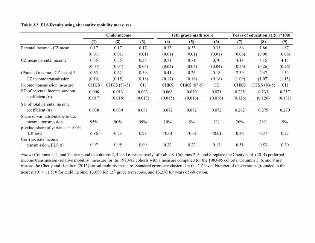
Table A2. ELS Results using alternative mobility measures

(1) (2) (3) (4) (5) (6) (7) (8) (9)Parental income - CZ mean 0.17 0.17 0.17 0.33 0.33 0.33 1.86 1.86 1.87

(0.01) (0.01) (0.01) (0.01) (0.01) (0.01) (0.06) (0.06) (0.06)CZ mean parental income 0.35 0.35 0.35 0.71 0.71 0.70 4.14 4.15 4.17

(0.04) (0.04) (0.04) (0.04) (0.04) (0.04) (0.26) (0.26) (0.26)(Parental income - CZ mean) * 0.65 0.62 0.59 0.41 0.26 0.18 2.39 2.47 1.54 CZ income transmission (0.16) (0.15) (0.18) (0.17) (0.16) (0.18) (1.09) (1.07) (1.15)Income transmission measure CHKS CHKS (83-5) CH CHKS CHKS (83-5) CH CHKS CHKS (83-5) CH

0.008 0.013 0.003 0.068 0.070 0.071 0.225 0.233 0.257(0.017) (0.018) (0.017) (0.015) (0.016) (0.016) (0.126) (0.126) (0.131)

SD of total parental income coefficient (S) 0.038 0.039 0.031 0.072 0.072 0.072 0.262 0.275 0.270Share of var. attributable to CZ income transmission 95% 90% 99% 10% 5% 2% 26% 28% 9%p-value, share of variance = 100% (LR test) 0.86 0.73 0.98 <0.01 <0.01 <0.01 0.36 0.37 0.27Corr(tax data income transmission, ELS S) 0.97 0.95 0.99 0.32 0.22 0.13 0.51 0.53 0.30

Child income 12th grade math score Years of education at 26 (*100)

Notes : Columns 1, 4, and 7 correspond to columns 2, 4, and 6, respectively, of Table 8. Columns 2, 5, and 8 replace the Chetty et al. (2014) preferred income transmission (relative mobility) measure for the 1980-82 cohorts with a measure computed for the 1983-85 cohorts. Columns 3, 6, and 9 use instead the Chetty and Hendren (2015) causal mobility measure. Standard errors are clustered at the CZ level. Number of observations (rounded to the nearest 10) = 11,510 for child income, 13,650 for 12th grade test scores, and 13,250 for years of education.

SD of parental income random coefficient (K)

Table A3. Parental income - child outcome relationships in the ELS, adding controls for race and gender

(1) (2) (3) (4) (5) (6) (7) (8) (9)Parental income - CZ mean 0.17 0.15 0.14 0.33 0.28 0.28 1.86 1.73 1.73

(0.01) (0.01) (0.01) (0.01) (0.01) (0.01) (0.06) (0.06) (0.06)CZ mean parental income 0.35 0.29 0.28 0.71 0.58 0.58 4.14 3.78 3.79

(0.04) (0.03) (0.04) (0.04) (0.04) (0.04) (0.26) (0.28) (0.28)(Parental income - CZ mean) * 0.65 0.44 0.38 0.41 0.13 0.20 2.39 2.00 2.18 CZ income transmission (0.16) (0.15) (0.16) (0.17) (0.16) (0.18) (1.09) (0.97) (1.02)SD of parental income random coefficient (K) 0.01 0.00 0.00 0.07 0.06 0.06 0.23 0.18 0.18

(0.02) (0.01) (0.02) (0.02) (0.02) (0.02) (0.13) (0.14) (0.15)Race and gender X X X X X XRace and gender X income transmission X X XSD of total parental income coefficient (S) 0.038 0.025 0.022 0.072 0.057 0.058 0.262 0.215 0.216Share of var. attributable to CZ income transmission 95% 99% 99% 10% 2% 4% 26% 27% 32%p-value, share of variance = 100% (LR test) 0.86 0.99 0.99 <0.01 0.02 0.02 0.36 0.22 0.23Corr(tax data income transmission, ELS S) 0.97 0.99 0.99 0.32 0.13 0.19 0.51 0.52 0.57

Child income 12th grade math score Years of education at 26 (*100)

Notes : Columns 1, 4, and 7 correspond to columns 2, 4, and 6, respectively, of Table 8. Columns 2, 5, and 8 add indicators for black, Hispanic, and female; columns 3, 6, and 9 also add interactions of these variables with CZ-level income transmission. Standard errors are clustered at the CZ level. Number of observations (rounded to the nearest 10) = 11,510 for child income, 13,650 for 12th grade test scores, and 13,250 for years of education.

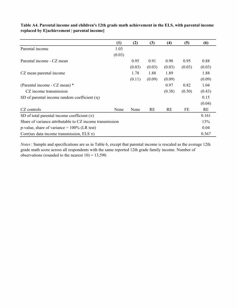
(1) (2) (3) (4) (5) (6)Parental income 1.03

(0.03)Parental income - CZ mean 0.95 0.91 0.90 0.95 0.88

(0.03) (0.03) (0.03) (0.03) (0.03)CZ mean parental income 1.78 1.88 1.89 1.88

(0.11) (0.09) (0.09) (0.09)(Parental income - CZ mean) * 0.97 0.82 1.04

CZ income transmission (0.38) (0.50) (0.43)SD of parental income random coefficient (K) 0.15

(0.04)CZ controls None None RE RE FE RESD of total parental income coefficient (S) 0.161Share of variance attributable to CZ income transmission 13%p-value, share of variance = 100% (LR test) 0.04Corr(tax data income transmission, ELS S) 0.367

Table A4. Parental income and children's 12th grade math achievement in the ELS, with parental income replaced by E[achievement | parental income]

Notes : Sample and specifications are as in Table 6, except that parental income is rescaled as the average 12th grade math score across all respondents with the same reported 12th grade family income. Number of observations (rounded to the nearest 10) = 13,590.

Table A5. Parental income - child outcome relationships in the ELS, using predicted parent income

(1) (2) (3) (4) (5) (6)Parental income - CZ mean 0.17 0.24 0.33 0.63 1.86 3.97

(0.01) (0.02) (0.01) (0.02) (0.06) (0.10)CZ mean parental income 0.35 0.48 0.71 1.11 4.14 6.28

(0.04) (0.05) (0.04) (0.06) (0.26) (0.40)(Parental income - CZ mean) * 0.65 1.46 0.41 0.49 2.39 2.45 CZ income transmission (0.16) (0.27) (0.17) (0.30) (1.09) (1.89)

0.01 0.10 0.07 0.10 0.23 0.43(0.02) (0.03) (0.02) (0.02) (0.13) (0.21)

Parental income measure Actual Pred. Actual Pred. Actual Pred.Number of observations (rounded to nearest 10) 11,510 10,950 13,650 12,880 13,250 12,570SD of total parental income coefficient (S) 0.038 0.127 0.072 0.100 0.262 0.455Share of variance attributable to CZ income transmission 95% 42% 10% 8% 26% 9%p-value, share of variance = 100% (LR test) 0.86 0.01 <0.01 <0.01 0.36 0.10Corr(tax data income transmission, ELS S) 0.97 0.65 0.32 0.28 0.51 0.30

Child income 12th grade math score

Years of education at 26 (*100)

Notes : Specifications in columns 1, 3, and 5 are those in Table 4, column 6; Table 6, column 6; and Table 8, column 6, respectively. Columns 2, 4, and 6 replace the parental income measure with predicted parental income, as in Table 4, column 6. Standard errors are clustered at the CZ level.

SD of parental income random coefficient (K)

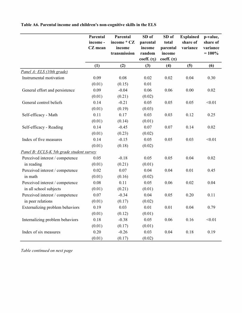
Table A6. Parental income and children's non-cognitive skills in the ELS

Parental income - CZ mean

Parental income * CZ

income transmission

SD of parental income random coeff. (K)

SD of total

parental income

coeff. (S)

Explained share of variance

p-value, share of variance = 100%

(1) (2) (3) (4) (5) (6)Panel A: ELS (10th grade)Instrumental motivation 0.09 0.08 0.02 0.02 0.04 0.30

(0.01) (0.15) 0.01General effort and persistence 0.09 -0.04 0.06 0.06 0.00 0.02

(0.01) (0.21) (0.02)General control beliefs 0.14 -0.21 0.05 0.05 0.05 <0.01

(0.01) (0.19) (0.03)Self-efficacy - Math 0.11 0.17 0.03 0.03 0.12 0.25

(0.01) (0.14) (0.01)Self-efficacy - Reading 0.14 -0.45 0.07 0.07 0.14 0.02

(0.01) (0.23) (0.02)Index of five measures 0.14 -0.15 0.05 0.05 0.03 <0.01

(0.01) (0.18) (0.02)Panel B: ECLS-K 5th grade student surveyPerceived interest / competence 0.05 -0.18 0.05 0.05 0.04 0.02 in reading (0.01) (0.21) (0.01)Perceived interest / competence 0.02 0.07 0.04 0.04 0.01 0.45 in math (0.01) (0.16) (0.02)Perceived interest / competence 0.08 0.11 0.05 0.06 0.02 0.04 in all school subjects (0.01) (0.21) (0.01)Perceived interest / competence 0.07 -0.34 0.04 0.05 0.20 0.11 in peer relations (0.01) (0.17) (0.02)Externalizing problem behaviors 0.19 0.03 0.01 0.01 0.04 0.79

(0.01) (0.12) (0.01)Internalizing problem behaviors 0.18 -0.38 0.05 0.06 0.16 <0.01

(0.01) (0.17) (0.01)Index of six measures 0.20 -0.26 0.03 0.04 0.18 0.19

(0.01) (0.17) (0.02)

Table continued on next page

Table A6 (continued)

Parental income - CZ mean

Parental income * CZ

income transmission

SD of parental income random coeff. (K)

SD of total

parental income

coeff. (S)

Explained share of variance

p-value, share of variance = 100%

(1) (2) (3) (4) (5) (6)Panel C: ECLS-K 5th grade teacher surveyApproaches to learning 0.19 0.58 0.06 0.07 0.25 0.02

(0.01) (0.18) (0.02)Self-control 0.15 0.72 0.06 0.08 0.32 0.02

(0.01) (0.18) (0.02)Interpersonal skills 0.15 0.22 0.05 0.05 0.06 0.16

(0.01) (0.17) (0.02)Peer relations 0.15 0.52 0.06 0.06 0.24 0.03

(0.01) (0.18) (0.01)Externalizing problem behaviors 0.11 0.48 0.03 0.04 0.50 0.05

(0.01) (0.12) (0.02)Internalizing problem behaviors 0.11 -0.02 0.07 0.07 0.00 <0.01

(0.01) (0.20) (0.01)Index of six measures 0.21 0.61 0.07 0.08 0.23 0.02

(0.01) (0.21) (0.02)

Notes : Each row presents a single mixed model regression, estimated without sampling weights. Dependent variables are discrete responses, scaled so that higher numbers are better and then converted to percentiles between 0 and 100 (with discrete responses assigned to the midpoint of the relevant range). Indexes are constructed by reversing the original response scale as necessary, converting to z-scores, averaging across responses and then converting to percentiles. Standard errors are clustered at the CZ level.

Table A7. Parent income - child income relationships in the ELS by gender

Child family income

Marital status (0/100)

Working spouse (0/100)

Child earnings

Child earnings + nonlabor income

Child earnings + non-labor income + imputed spousal

earnings

(1) (2) (3) (4) (5) (6)Panel A: Men

Parental income - CZ mean 0.17 -0.08 -0.02 0.14 0.18 0.15(0.03) (0.03) (0.03) (0.03) (0.03) (0.03)

CZ mean parental income 0.31 -0.03 0.15 0.21 0.29 0.30(0.06) (0.14) (0.13) (0.06) (0.06) (0.07)

(Parental income - CZ mean) * 1.30 1.22 1.00 0.72 0.91 1.26 CZ income transmission (0.43) (0.55) (0.61) (0.48) (0.44) (0.44)

0.13 0.05 0.09 0.16 0.14 0.13(0.04) (0.05) (0.13) (0.04) (0.03) (0.04)

SD of total parental income coefficient (S) 0.147 0.086 0.103 0.169 0.149 0.144Share of variance attributable to CZ income transmission 25% 65% 30% 6% 12% 24%p-value, share of variance = 100% (LR test) 0.16 0.60 0.67 <0.01 0.02 0.15Corr(tax data income transmission, ELS S) 0.50 0.80 0.55 0.24 0.35 0.49

Panel B: WomenParental income - CZ mean 0.31 0.02 0.05 0.28 0.33 0.28

(0.02) (0.04) (0.03) (0.02) (0.02) (0.02)CZ mean parental income 0.66 0.00 0.07 0.63 0.66 0.56

(0.08) (0.14) (0.14) (0.06) (0.06) (0.08)(Parental income - CZ mean) * 1.33 1.25 1.21 0.76 0.74 1.51 CZ income transmission (0.42) (0.56) (0.58) (0.38) (0.39) (0.40)

0.10 0.07 0.04 0.08 0.07 0.09(0.04) (0.13) (0.19) (0.05) (0.04) (0.04)

SD of total parental income coefficient (S) 0.127 0.098 0.078 0.089 0.085 0.125Share of variance attributable to CZ income transmission 35% 52% 76% 23% 24% 46%p-value, share of variance = 100% (LR test) 0.07 0.94 0.81 0.36 0.46 0.09Corr(tax data income transmission, ELS S) 0.59 0.72 0.87 0.48 0.49 0.68

SD of parental income random coefficient (K)

SD of parental income random coefficient (K)

Notes : Sample and specifications are as in Table 5, but with models estimated separately by gender. N (rounded to the nearest 10) = 5,090 in Panel A; 5,850 in Panel B.

Mechanism Total transmission

Skills Return to skills

Residual Non-labor and spousal income

Dependent variable Child income Child skill

index

Child earnings

Child earnings residual

Family income less own earnings

(1) (2) (3) (4) (5)Panel A: Men

Parental income - CZ mean 0.13 0.09 0.03 0.03(0.01) (0.00) (0.01) (0.01)

CZ mean parental income 0.23 0.19 0.02 0.04(0.04) (0.01) (0.04) (0.02)

CZ income transmission 7.55 -2.23 7.59 -1.37 -1.70(10.52) (2.41) (8.53) (8.59) (4.91)

(Parental income - CZ mean) * 0.53 0.10 0.08 0.23CZ income transmission (0.23) (0.06) (0.22) (0.11)

Skill index - CZ mean 0.77(0.06)

CZ mean skill index 0.86(0.12)

(Skill index - CZ mean) * CZ income transmission 2.01(1.01)

d skills index / d parental income (scale factor) 0.09Scaled component 0.53 0.10 0.17 0.08 0.23

100% 19% 33% 15% 44%

Table continued on next page

Table A8. Decomposition of the variation in intergenerational income transmission using child earnings by gender

Share of total

Mechanism Total transmission

Skills Return to skills

Residual Non-labor and spousal income

Dependent variable Child income Child skill

index

Child earnings

Child earnings residual

Family income less own earnings

(1) (2) (3) (4) (5)Panel B: Women

Parental income - CZ mean 0.19 0.09 0.06 0.03(0.01) (0.00) (0.01) (0.01)

CZ mean parental income 0.42 0.19 0.12 -0.04(0.05) (0.01) (0.03) (0.04)

CZ income transmission -6.09 -6.75 11.10 -4.17 -9.87(9.53) (1.95) (6.78) (4.25) (9.80)

(Parental income - CZ mean) * 0.64 0.04 0.25 0.29CZ income transmission (0.24) (0.08) (0.17) (0.16)

Skill index - CZ mean 1.14(0.05)

CZ mean skill index 1.66(0.13)

(Skill index - CZ mean) * CZ income transmission 0.16(0.78)

d skills index / d parental income (scale factor) 0.090.64 0.04 0.01 0.25 0.29

Share of total 100% 7% 2% 39% 45%

Table A8 (continued)

Scaled component

Notes : Sample and specifications are as in Table 11, but with models estimated separately by gender. N = 4,630 in Panel A; 5,350 in Panel B.