Inequality, Leverage and Crises

Michael Kumhof and Romain Rancière

WP/10/268

© 2010 International Monetary Fund WP/10/268 IMF Working Paper Research Department

Inequality, Leverage and Crises

Prepared by Michael Kumhof and Romain Rancière

Authorized for distribution by Douglas Laxton

November 2010

Abstract

This Working Paper should not be reported as representing the views of the IMF. The views expressed in this Working Paper are those of the author(s) and do not necessarily represent those of the IMF or IMF policy. Working Papers describe research in progress by the author(s) and are published to elicit comments and to further debate.

The paper studies how high leverage and crises can arise as a result of changes in the income distribution. Empirically, the periods 1920-1929 and 1983-2008 both exhibited a large increase in the income share of the rich, a large increase in leverage for the remainder, and an eventual financial and real crisis. The paper presents a theoretical model where these features arise endogenously as a result of a shift in bargaining powers over incomes. A financial crisis can reduce leverage if it is very large and not accompanied by a real contraction. But restoration of the lower income group's bargaining power is more effective. JEL Classification Numbers: E20; E25. Keywords: Income inequality; consumption inequality; income distribution; distributional

conflict; leverage; financial crises; default risk; global solution methods. Author’s E-Mail Address: mkumhof@imf.org, rranciere@imf.org

2

Contents

I. Introduction . . . . . . . . . . . . . . . . . . . . . . . . . . . . . . . . . . . . . . 3

II. Stylized Facts . . . . . . . . . . . . . . . . . . . . . . . . . . . . . . . . . . . . . 5

III. The Model . . . . . . . . . . . . . . . . . . . . . . . . . . . . . . . . . . . . . . 8

A. Investors . . . . . . . . . . . . . . . . . . . . . . . . . . . . . . . . . . . . 8

B. Workers . . . . . . . . . . . . . . . . . . . . . . . . . . . . . . . . . . . . . 10

C. Technology . . . . . . . . . . . . . . . . . . . . . . . . . . . . . . . . . . . 11

D. Equilibrium . . . . . . . . . . . . . . . . . . . . . . . . . . . . . . . . . . . 12

E. Calibration . . . . . . . . . . . . . . . . . . . . . . . . . . . . . . . . . . . 12

F. Solution Methods . . . . . . . . . . . . . . . . . . . . . . . . . . . . . . . 13

IV. Simulated Scenarios . . . . . . . . . . . . . . . . . . . . . . . . . . . . . . . . . 15

A. Baseline Scenario . . . . . . . . . . . . . . . . . . . . . . . . . . . . . . . 15

B. Uncertainty . . . . . . . . . . . . . . . . . . . . . . . . . . . . . . . . . . . 17

C. High Leverage - Aggravating Factors . . . . . . . . . . . . . . . . . . . . . 17

D. High Leverage - Solutions . . . . . . . . . . . . . . . . . . . . . . . . . . . 20

E. Further Discussion . . . . . . . . . . . . . . . . . . . . . . . . . . . . . . . 21

V. Conclusions . . . . . . . . . . . . . . . . . . . . . . . . . . . . . . . . . . . . . . 22

References . . . . . . . . . . . . . . . . . . . . . . . . . . . . . . . . . . . . . . . . . . 23

Figures

1. Income Inequality and Household Leverage . . . . . . . . . . . . . . . . . . . . . 26

2. Real Income Inequality . . . . . . . . . . . . . . . . . . . . . . . . . . . . . . . . 27

3. Income Inequality and Consumption Inequality . . . . . . . . . . . . . . . . . . . 28

4. The Variance of Annual, Permanent, and Transitory (log) Earnings . . . . . . . . . 28

5. Debt to Income Ratios . . . . . . . . . . . . . . . . . . . . . . . . . . . . . . . . 29

6. The Size of the U.S. Financial Sector . . . . . . . . . . . . . . . . . . . . . . . . 29

7. Mortgage Debt and Subprime Borrowing . . . . . . . . . . . . . . . . . . . . . . 30

8. Mortgage Default - Share of Past Due Loans . . . . . . . . . . . . . . . . . . . . 31

9. Leverage and Crisis Probability in the Model . . . . . . . . . . . . . . . . . . . . 31

10. Baseline Scenario . . . . . . . . . . . . . . . . . . . . . . . . . . . . . . . . . . . 32

11. Less Capital Investment . . . . . . . . . . . . . . . . . . . . . . . . . . . . . . . 33

12. Nearly Permanent Change in Bargaining Power . . . . . . . . . . . . . . . . . . . 34

13. High Variable instead of Low Fixed Subsistence Consumption . . . . . . . . . . . 35

14. Orderly Debt Restructuring . . . . . . . . . . . . . . . . . . . . . . . . . . . . . . 36

15. Restoration of Workers’ Bargaining Power . . . . . . . . . . . . . . . . . . . . . 37

3

I. INTRODUCTION

The United States experienced two major economic crises over the past century—the Great

Depression starting in 1929 and the Great Recession starting in 2007. Both were preceded by

a sharp increase in income and wealth inequality, and by a similarly sharp increase in

debt-to-income ratios among lower- and middle-income households. When those

debt-to-income ratios started to be perceived as unsustainable, it became a trigger for the

crisis. In this paper, we first document these facts, and then present a dynamic stochastic

general equilibrium model in which a crisis driven by income inequality can arise

endogenously. The crisis is the ultimate result, after a period of decades, of a shock to the

relative bargaining powers over income of two groups of households, investors who account

for 5% of the population, and whose bargaining power increases, and workers who account

for 95% of the population.

The model is kept as simple as possible in order to allow for a clear understanding of the

mechanisms at work. The key mechanism is that investors use part of their increased income

to purchase additional financial assets backed by loans to workers. By doing so, they allow

workers to limit their drop in consumption following their loss of income, but the large and

highly persistent rise of workers’ debt-to-income ratios generates financial fragility which

eventually can lead to a financial crisis. Prior to the crisis, increased saving at the top and

increased borrowing at the bottom results in consumption inequality increasing significantly

less than income inequality. Saving and borrowing patterns of both groups create an increased

need for financial services and intermediation. As a consequence the size of the financial

sector, as measured by the ratio of banks’ liabilities to GDP, increases. The crisis is

characterized by large-scale household debt defaults and an abrupt output contraction as in the

2007 U.S. financial crisis. Because crises are costly, redistribution policies that prevent

excessive household indebtedness and reduce crisis-risk ex-ante can be more desirable from a

macroeconomic stabilization point of view than ex-post policies such as bailouts or debt

restructurings. To our knowledge, our framework is the first to provide an internally consistent

mechanism linking the empirically observed rise in income inequality between high income

households and poor to middle income households, the increase in household debt-to-income

ratios among the latter group, and the risk of a financial crisis.

This paper integrates two strands of literature that have largely been evolving separately: the

literature on income and wealth distribution and the literature on financial fragility and

macroeconomic volatility. The first literature is mostly focused on accurately describing long

run changes in the distribution of income and wealth (Piketty and Saez (2003), Piketty

(2010)). One of its main findings is that the most significant changes in the income

distribution concern the evolution of top income shares. This feature is taken on board in our

model, where income heterogeneity is introduced by considering two groups representing the

top stratum and the remainder of the income distribution.

4

A companion literature in labor economics seeks to uncover the fundamental factors shaping

the change in the income distribution in the United States over the last thirty years. Lemieux,

MacLeod and Parent (2009) find that an increase in the share of performance pay (e.g.

bonuses) can explain 20% of the growth in the variance of male wages between the late 1970s

and the early 1990s, and almost all of the growth in wage inequality at the very top end of the

income distribution. Lemieux (2006) shows that the dramatic increase in the return to

post-secondary education plays an important role in the increase in income inequality and can

explain why wage gains are disproportionately concentrated at the top of the distribution.

Card, Lemieux and Riddell (2004) find that changes in unionization can explain around 14%

of the growth in the variance of male earnings in the United States. Finally, Borjas and Ramey

(1995) and Roberts (2010) point to the role of foreign competition and jobs offshoring in the

rise of income inequality.

Our paper focuses only on the macroeconomic implications of increased income inequality.

Therefore, rather than taking a stand on the microeconomic reasons for that increase, it

represents more fundamental shocks by way of a shock to the relative bargaining powers of

the two income groups. A similar reduced-form modeling device is employed by Blanchard

and Giavazzi (2003), where labor market deregulation is formalized as a reduction in the

bargaining power of workers.

The literature on financial fragility has so far ignored the role of income heterogeneity in

creating crisis risk. In the canonical Diamond and Dybvig (1983) crisis model, the

heterogeneity that matters is that between patient and inpatient consumers. Differences

between impatient and patient consumers also feature prominently in financial accelerator

models applied to household debt and housing cycles (Iacoviello (2005, 2008)). In this paper

we argue that, because increases in household debt-to-income ratios, which increase financial

fragility, have been strongly heterogenous across income groups, as documented in Section II,

heterogeneity in incomes is a key additional feature that should be explored in models of

household debt and financial crises.

While not formally modeled there, the link between income inequality, household

indebtedness and crises has been recently discussed in opinion editorials by Paul Krugman,

and in books by Rajan (2010) and Reich (2010). Both authors suggest that increases in

borrowing have been a way for the poor and the middle-class to maintain or increase their

level of consumption at times when their real earnings were stalling. But these authors do not

make a formally consistent case for that argument. Our model allows us to do so.

There are of course other candidate explanations for the origins of the 2007 crisis, and many

have stressed the roles of excessive financial liberalization and of asset price bubbles.1

Typically these factors are found to have been important in the final years preceding the crisis,

1Keys, Mukherjee, Seru and Vig (2010) discuss the adverse effects of increased securitization on systemic risk.

Taylor (2009) claims that the interaction of unusually easy monetary policy with excessive financial liberalization

5

when debt-to-income ratios increased more steeply than before. But it can also be argued, as

done in Rajan (2010), that much of this was simply a manifestation of an underlying and

longer-term dynamics driven by income inequality. Rajan’s argument is that growing income

inequality created political pressure, not to reverse that inequality, but instead to encourage

easy credit to keep demand and job creation robust despite stagnating incomes.

It has also been suggested that the increase in wealth of the richest households has played a

role in increasing the demand for investment assets. In our model, the financial sector

intermediates funds between the increasingly richer top fraction of the population and the

increasingly more indebted bottom fraction of the population. As the flow of funds between

the two groups increases, so does the size of the financial sector as measured by total assets or

total liabilities over GDP. This fact is consistent with recent findings by Philippon (2008). The

size of the demand by the top 5% for bank deposits, in other words for assets backed by

household debt, is quantified by directly introducing wealth into their preferences, reflecting a

"capitalist spirit" motive stressed by a number of authors starting with Carroll (2000).

A recent literature has attempted to relate the rise in income inequality to the increase in

household debt (Krueger and Perri (2006), Iacoviello (2008)). There is an important

difference between our approach and that followed by these authors. In their approach an

increase in the variance of idiosyncratic income shocks across all households generates a

higher demand for insurance in credit markets, thereby increasing household debt. Their

approach therefore emphasizes an increase in income inequality experienced equally within

each household group, while our paper focuses on the rise in income inequality between two

household groups. There is a lively academic debate concerning the relative roles of within-

and between-group factors in shaping inequality. But our paper only focuses on one specific

type of between-group inequality that can be clearly documented in the data, namely

inequality between high income households and everyone else.

The rest of the paper is organized as followed. Section II presents a number of key stylized

facts. Section III presents the model. Section IV presents model simulations to study the

effects of increasing income inequality, and to discuss policy implications. Section V

concludes.

II. STYLIZED FACTS

This section documents a number of key stylized facts regarding the evolution of the

distribution of income, wealth and consumption, changes in household debt-to-income ratios

overall and for different groups, the size of the financial sector, and household debt default

caused the crisis. Obstfeld and Rogoff (2009) claim that the interaction of these factors with global current account

imbalances helped to create a “toxic mix” that helped to set off a worldwide crisis.

6

risk during the financial crisis of 2007. The model presented in the next section will be

calibrated to broadly replicate these facts.

Income Inequality and Household Debt: 1929 vs. 2007

Figure 1 plots the evolution of income inequality and household debt ratios in the two decades

preceding the two major U.S. crises - 1929 and 2007. In both periods income inequality

experienced a sharp increase of similar magnitude: the share of total income (excluding

capital gains) commanded by the top 5% of the income distribution increased from 24% in

1920 to 34% in 1928, and from 22% in 1983 to 34% in 2007. During the same two periods,

the ratio of household debt to GNP or to GDP increased dramatically. It almost doubled

between 1920 and 1932, and also between 1983 and 2007, when it reached much higher levels

than in 1932. In short the joint evolution of income inequality across high and low income

groups on the one hand, and of household debt-to-income ratios on the other hand, displays a

remarkably similar pattern in both pre-crisis eras.

Income Inequality and Consumption Inequality

In order to model the consequences of rising income inequality, it is important to clearly

document the respective dynamics of income inequality, consumption inequality and wealth

inequality. To do so we use a recent comprehensive dataset compiled by Heathcote, Perri and

Violante (2010).2

Figure 2, top panel, plots the cumulative percentage changes of male hourly real wages

between 1967 and 2005 for three deciles of the distribution of wage earnings: the bottom 10

percentile, the percentile surrounding the median, and the top 10 percentile. Figure 2, bottom

panel, plots the cumulative percentage change in real male annual earnings for the same three

deciles. Both graphs illustrate the large widening of wage inequality over recent decades. The

real hourly wages of the top 10 percentile increased sharply by a cumulative 70%, the real

hourly wages around the median declined by 5%, while the wages of the bottom 10%

declined strongly, by around 25%. The widening in earnings inequality is even more

pronounced when annual earnings are considered reflecting the role of hours and

unemployment in the bottom percentile. In the context of our theoretical framework, we take

this change in the relative distribution of earnings as the key shock to our model economy.

Figure 3 documents the evolution of inequality in disposable incomes and in non-durable

consumption between 1980 and 2006. The graph plots the ratio of disposable incomes and the

ratio of non-durable consumption levels between the top and the bottom 10 percentile of the

disposable income distribution. An important finding, already stressed by Slescnik (2001) and

Krueger and Perri (2006), is that the rise in income inequality has been much more

pronounced than the increase in consumption inequality.

2The rise in U.S. income inequality has been documented since at least Gottshalk and Moffit (1994).

7

Income Mobility

To better understand the differences between income inequality and consumption inequality, it

is important to assess the importance of intra-generational income mobility. In theory, if

increasing income inequality was accompanied by an increase in income mobility, the

dispersion in lifetime earnings might be much smaller than the dispersion in annual earnings,

as agents move up and down the income ladder throughout their lives. This is a potential

explanation for why consumption inequality has been lower than income inequality. However,

the data show that, if anything, income mobility has been declining in the United States over

the last 40 years, particularly mobility between the top income group and the remainder that

we care about in this paper.

A recent study by Kopczuk, Saez and Song (2010)3, using micro-level social security data

with the sample restricted to men, shows that measures of short-term income mobility

(mobility at a five year horizon) and long-term income mobility (lifetime mobility) have been

either stable or slightly worsening since the 1950s. As a consequence the evolution of annual

income inequality over time is very close to the evolution of longer-term income inequality.

They also find that the surge in top earnings is not due to increased mobility between the top

income group and other groups. The probability of staying among the top 1% of earnings

after 1,3 or 5 years shows no overall trend since the top share started to be coded in Social

Security Data (1978).

In addition, Kopczuk, Saez and Song (2010) show that increases in the variance of annual

earnings have been due to increases in the variance of permanent earnings, with only modest

increases in the variance of transitory earnings. Figure 4, which uses their data, illustrates this

result by plotting, starting in 1970, the variance of annual log earnings, the variance of

five-year log earnings (the permanent variance) and the variance of the five-year log earnings

deviation (the transitory variance).

These findings together provide support for one of our key simplifying modeling choices, the

assumption of two income groups with essentially fixed memberships.

Wealth Inequality and Household Debt-to-Income Ratios

In the absence of any change in the valuation of household assets and liabilities, a smaller

increase in consumption inequality relative to income inequality must imply that households

at the bottom of the distribution of income and wealth are becoming more indebted than

households at the top. Figure 5 shows the evolution of debt-to-income ratios for the top 5%

and bottom 95% of households, this time ranked by wealth rather than income, between 1983

and 2007. In 1983, the top wealth group is somewhat more indebted than the bottom group,

with a gap of around 15 percentage points. In 2007, the relative debt situation is dramatically

3See also Bradbury and Katz (2002).

8

reversed: the debt-to-income ratio of the bottom group, at around 140%, is now twice as high

as the debt-to-income ratio of the top group. Between 1983 and 2007, the debt-to-income

ratio of the bottom group has therefore more than doubled while the ratio of the top group has

remained fluctuating around 70%. As a consequence almost all of the increase in the

debt-to-income ratio at the aggregate level comes from the bottom group of the wealth

distribution. Once again this provides very strong motivation for introducing income

heterogeneity into a model of household indebtedness and financial fragility.

The Size of the U.S. Financial Sector

In our theoretical framework, the increase in debt of the bottom 95% of the distribution

generates an increasing need for financial intermediation. Figure 6 plots two measures of the

size of the U.S. financial sector between 1980 and 2007. The left panel plots the standard

measure of private credit by deposit banks and other financial institutions to GDP. It more

than doubled over the period, increasing from 90% in 1981 to 210% in 2007. The right panel

plots the share of the financial sector in GDP as constructed by Philippon (2010). According

to this measure the financial sector almost doubled in size between 1981 and 2007, and most

recently accounted for an extraordinary 8% of U.S. GDP. A similar pattern was again

observed prior to the Great Depression.

Debt-to-Income Ratios, Risk and Financial Crises

As shown in Figure 7, top panel, most of the increase in debt-to-income ratios for the bottom

95% group in the period preceding the crisis was associated with mortgage debt. In the

mortgage market, the growing share of subprime loans as documented in Figure 7, bottom

panel, is an indicator of the increased riskiness that has accompanied higher indebtedness.

Figure 8 shows evidence of an increase in mortgage debt default risk following 2007 of a

magnitude unprecedented since the Great Depression. Default probabilities that increase with

debt-to-income ratios, and default rates of the magnitude observed recently, are key

ingredients of our model and its calibration.

III. THE MODEL

The model economy consists of two groups of households, referred to as investors and

workers, and of a production technology that combines the inputs provided by investors and

workers.

A. Investors

The share of investors in the overall population equals χ, which we will calibrate at 5%. They

derive utility from consumption and wealth.

9

Utility from consumption cit has the standard CRRA form, with intertemporal elasticity of

substitution σi, but is subject to a subsistence, or minimum acceptable, level of consumption

cimin. The interpretation of subsistence consumption is that most individuals have arranged

their affairs in such a manner that a precipitous drop in consumption would be disastrous,

such as a drastic loss of status or, in the case of workers below, destitution and homelessness.

Wealth in the utility function has been used by a number of authors including Carroll (2000),

who refers to it as the “capitalist spirit” specification, Reiter (2004), and Piketty (2010). As

explained by the latter, it can represent a number of different saving motives. One is as a

reduced form for precautionary savings, because wealth provides security in the presence of

uninsurable lifetime shocks. Our preferred interpretation is that agents derive direct utility

from the prestige, power and social status conferred by wealth.4 Wealth in our model can take

two forms, physical capital held from period t to t+ 1 and denoted by kt, and financial

investments, or deposits, held from t to t+ 1 and denoted by dt. Utility from deposits is

assumed to take the log-form that is common in studies of money demand, but adjusted for

expected losses from a crisis event. Utility from physical capital is assumed to take a

Stone-Geary form, with utility derived from the logarithm of the sum of physical capital,

adjusted for expected losses from a crisis event, and a constant k that determines the

sensitivity of desired capital investment to changes in income. We will study how our results

depend on the value taken by k. Losses from a crisis event depend on the probability of a

crisis in t+ 1, πt, which is taken as given by households, known by time t, and which will be

discussed further below. It also depends on the percentage of the loan or capital stocks

destroyed in the event of a crisis, (1− γℓ) and (1− γk). The expected loan and capital stocks

therefore equal dt (1− (1− γℓ) πt) and kt (1− (1− γk) πt), and we have the lifetime utility

function

U i0 = E0

∞∑

t=0

βti

(cit − c

imin)

(1−

1

σi

)

(1− 1

σi

) + ξd log (dt (1− (1− γℓ) πt)) + ξk log(k + kt (1− (1− γk) πt)

)

.

(1)

Investors are the owners of the economy’s entire stock of physical capital, whose law of

motion is given by

kt = (1− δ)∆ktkt−1 + It . (2)

Here It represents physical investment, and ∆kt equals γk < 1 in the event of a crisis, and 1

otherwise. We assume that investors do not engage in wage labor, and instead derive all of

their income from their ownership of the physical capital stock and from interest on loans to

workers. This assumption is made to keep the model parsimonious, but it is not strictly

necessary for our main results and could be relaxed to allow for some wage labor in this

4Carroll (2000) argues that this wealth-loving motive is the best explanation for why saving rates increase so

dramatically with the level of lifetime income. See also Dynan, Skinner and Zeldes (2004) and Kopczuk (2007).

10

sector. We let qt be the time t price of a deposit that pays off one unit of output in period t+1,

∆ℓt equals γℓ < 1 in the event of a crisis and 1 otherwise, and we denote the return to capital

kt−1 by rkt . Then the investor’s budget constraint is given by

dtqt = ∆ℓtdt−1 + rkt∆ktkt−1 − c

it − It . (3)

Investors maximize (1) subject to (2) and (3). Letting λit be the multiplier of the budget

constraint, the optimality conditions for consumption, deposits and capital are given by

(cit − c

imin

)−

1

σi = λit , (4)

1 = βiEt

(λit+1λit

)(1− (1− γℓ)πt)

qt+

ξdλitdtqt

, (5)

1 = βiEt

(λit+1λit

)(rkt+1 + 1− δ

)(1− (1− γk)πt) +

ξk (1− (1− γk)πt)

λit(k + kt (1− (1− γk)πt)

) . (6)

B. Workers

The share of workers in the overall population equals 1− χ, which we will calibrate at 95%.

They derive utility from consumption, with the same CRRA form as investors’ consumption

utility. We use the same notation as for investors, with the index w replacing the index i.

Workers inelastically supply one unit of labor per capita. Lifetime utility is given by

Uw0 = E0

∞∑

t=0

βtw(cwt − c

wmin)

(1− 1

σw)

(1− 1

σw

) . (7)

Workers maximize this utility subject to the budget constraint

ℓtqt = ∆ℓtℓt−1 + cwt − wt , (8)

where ℓt denotes loans obtained from investors and wt is the real wage. Workers default on

their loan obligations with a positive probability πt that is increasing in their debt-to-income

ratio according to a logistic function. We will henceforth refer to the debt-to-income ratio as

leverage. Default events, or financial crises, are accompanied by real crises in which the

capital stock is impaired. We will therefore refer to πt not as the default probability but more

broadly as the crisis probability. Part of our analysis will consist of experiments that vary the

relative sizes of the financial and real components of crises.

The logistic function bounds the crisis probability between 0 and 1, and over the relevant

range it implies a crisis probability that is convex in leverage. The leverage that is relevant for

11

the probability of a crisis in period t+ 1 equals the ratio of workers’ loans outstanding at the

end of period t to their net income in period t, where the latter is defined as their time t wage

income minus their net interest obligations on loans outstanding between periods t and t+ 1.

We have

πt =

exp

(φ0 + φ1

(ℓt

wt−(1

qt−1

)ℓt

))

1 + exp

(φ0 + φ1

(ℓt

wt−(1

qt−1

)ℓt

)) . (9)

We adopt this specification in the interest of keeping the model simple and tractable.5 A

relationship between leverage and crisis probability such as (9) arises endogenously in crisis

models such as Schneider and Tornell (2004), where a high enough debt leverage moves the

economy to a risky zone where a roll-over debt crisis can occur with positive probability.

Workers’ optimality conditions for consumption and loans are given by

(cwt − cwmin)

−1

σw = λwt , (10)

1 = βwEt

(λwt+1λwt

)(1− (1− γℓ)πt)

qt. (11)

C. Technology

The economy’s aggregate production function is given by

yt = A(χ∆kt kt−1

)α(1− χ)1−α , (12)

where A is a scale factor that will be used to normalize the economy’s calibrated steady state

output level. Factor returns are determined by the outcome of a Nash bargaining problem over

the real wage. Denoting workers’ bargaining power by ηt, we have

Maxwt

(Wht)ηt (Kht)

1−ηt , (13)

whereWht = λwt wt is the workers’ surplus, andKht = fht − wt is the investors’ surplus. The

marginal product of labor fht is in turn given by

fht =(1− α) yt(1− χ)

. (14)

The first-order condition of the bargaining problem simplifies to

wt = ηtfht . (15)

5Davig, Leeper and Walker (2010) have, in a different context, adopted an almost identical approach. In their

paper the probability of collapse of an initial fiscal regime follows an exogenous logistic function that is increasing

in tax rates, and upon collapse the tax rate defaults to an exogenous constant value.

12

In other words, the real wage equals workers’ bargaining power times the marginal product of

labor. This implies that ηt can fall into the interval ηt ∈ [0,1−χ

1−α]. The standard competitive

outcome obtains at a bargaining power of one. We assume that workers’ bargaining power

follows an autoregressive stochastic process that is given by

ηt = (1− ρ) η + ρηt−1 + eηt . (16)

Finally, the expected rental rate of capital, which enters into the Euler equation for capital (6),

is given by

Et[rkt+1

]= Et

[A (χ (1− (1− γk)πt) kt)

α (1− χ)1−α(1− ηt+1 (1− α)

)

χ (1− (1− γk) πt) kt

]

. (17)

D. Equilibrium

In equilibrium investors and workers maximize their respective lifetime utilities, and the

following market clearing conditions for goods and for financial claims hold:

yt = χ(cit + It

)+ (1− χ) cwt , (18)

(1− χ) ℓt = χdt . (19)

E. Calibration

Because our study concerns longer-run phenomena, we calibrate the model at the annual

frequency. Utility from consumption takes an identical form across agents, with intertemporal

elasticities of consumption equal to σi = σw = 0.5. The subsistence level of consumption

equals 50% of initial steady-state consumption. The steady-state real interest rate ((1/q)− 1)

is fixed at 5% per annum, similar to values typically used by the RBC literature, by

endogenizing workers’ time preference βw. Given the presence of positive capitalist spirit

terms in the utility function of investors, βi = 0.9 is lower than βw. The utility weight on

financial wealth ξd is then determined by imposing an initial steady-state loans-to-income

ratio for workers of 64%, consistent with the U.S. value in 1983. The utility weight on

physical capital is determined by imposing an initial steady-state gross financial return to

capital of 15% per annum, equal to the sum of the real interest rate and the depreciation rate δ,

which equals 10% per annum. Finally, the Stone-Geary constant in the utility for physical

capital,which affects the elasticity of capital’s response to bargaining power shocks, is set at

k = −30. We will experiment with alternative values for k.

In the aggregate technology, we normalize steady-state output to one through our choice of

the parameter A. We set the capital share parameter equal to α = 0.27, which generates a

steady-state investment-to-GDP ratio of 18%, consistent with U.S. data. It also implies an

initial steady-state income share of investors of 29.8%. As mentioned in Section II, in the

13

United States this income share equalled 22% in the early 1980s and 34% in recent times. The

mean bargaining power η = 1 replicates the competitive outcome, and the standard deviation

of bargaining power shocks is assumed to equal ση = 0.015. As there is little guidance from

the literature regarding an appropriate value for ση, we will also present the perfect foresight

case ση = 0 in our simulations, so that the implications of intermediate values of ση can be

inferred by comparing the two simulations.

A crisis event is characterized by the probability of its occurrence, and by the size of the

collapses in loans and capital, and therefore in output, if it does occur. We set the two

coefficients of the logistic function to φ0 = −7.5 and φ1 = 3. As illustrated in Figure 9, this

produces a baseline crisis probability of 0.38% at a leverage of 64%, and a convex

relationship between leverage and the crisis probability that reaches almost 5% at a leverage

of 150%. This range is consistent with the probability of major disaster events estimated by

Barro (2006), who finds a range of 1%-2.5%, and by Rancière, Tornell and Westermann

(2008), who estimate 4% for the period 1980-2000.6 Next we calibrate the size of disaster

events, that is of major defaults on loans and of output collapses. Based on International

Monetary Fund (2009), the reductions in the level of output associated with major financial

crises that coincided with real crises have averaged 3.4%. We generate a comparable output

collapse by assuming capital destruction in the event of a crisis equal to 10% of the

pre-existing capital stock, γk = 0.9. Given the capital share parameter in the technology this

leads to an output collapse of around 2.7%. Clearly the ability of our simple model to

generate large output collapses is limited by the fact that it does not allow for increases in

unemployment at times of crises. To test the sensitivity of our results to the assumption of

γk = 0.9 we will also explore an alternative scenario where the capital destruction only equals

1%, or γk = 0.99. The percentage of loans defaulted upon during the crisis is based on the

U.S. experience, up to this point, with the financial crisis that started in 2007. This crisis has

seen mortgage past due rates approaching 10%. We therefore set γℓ = 0.9.

F. Solution Methods

The above model has two features that make it unsuitable for the application of conventional

perturbation methods. The first is the presence of large and discrete crisis events, which under

our calibration imply jumps in state variables of up to 10%. The second is the fact that the

model’s two endogenous state variables, capital and loans, are extremely persistent, and are

then subjected to large bargaining power shocks, which means that they can drift far away

from their original steady state for a very long period. It is therefore necessary to apply global

solution methods. We adopt and compare two different approaches.

6Applied to the 2007 crisis this quite low perceived probability seems appropriate given the evident surprise

of a majority of commentators at the outbreak of the crisis. It is a separate question whether this assessment

was realistic, given the historically unprecedented household leverage ratios in 2007, even when compared to the

Great Depression.

14

First, our model has three continuous state variables (capital, loans and bargaining power) and

one binary state variable (crisis or no crisis). This is sufficiently tractable to permit the use of

functional iteration on a discretized state space to compute solutions. Specifically, we use the

monotone map method of Coleman (1991), which has recently been used in a number of

papers by Davig, Leeper and Walker.7 The monotone map method discretizes the state space

and finds a fixed point in decision rules for each grid point in the state space. It substitutes a

set of conjectured decision rules into the model’s intertemporal Euler equations, and iterates

until the iteration improves the current decision rule at any given state vector by less than

some ε. As initial conjectures we use decision rules computed by DYNARE for a first-order

approximation of the model. These conjectures are applied to a version of the nonlinear

model with only a small fraction of the full standard deviation ση, and with a narrow grid for

the state space, based on the conjecture that for a sufficiently small standard deviation the

solutions are approximately linear. Both the standard deviation and the grid width are then

sequentially increased, and at each step the results of the previous iteration, appropriately

scaled up or down to account for the wider spacing of grid points, are used as initial guesses.

Numerical integration is used to compute expectations. As evidence of local uniqueness, we

perturb the converged decision rules in various dimensions and check that the algorithm

converges back to the same solution.

We present 50-year impulse responses for a standardized realization of bargaining power and

crisis shocks, namely an initial decline in workers’ bargaining power from η = 1 over a period

of 10 years, followed by a very gradual return to η = 1, and a crisis event in year 30. This can

be thought of as a highly stylized representation of the events preceding either 1929 or 2007.

Sensitivity analysis varies a number of aspects of this shock sequence, including the size of

the decline in bargaining power over the first 10 years, the speed of reversal to η = 1 after

year 10, the size of the crisis event, the perceived probability of a crisis event, the elasticity of

capital accumulation with respect to bargaining power shocks, and the form (fixed or variable)

of subsistence consumption.

We also use a second solution method, a perfect foresight solution in TROLL using a

Newton-based stacking algorithm8, and compare the monotone map simulations with the

corresponding perfect foresight simulations. The reason is that this comparison yields

interesting additional insights regarding the effects of uncertainty, and regarding the

quantitative implications of using different calibrated values for ση. In the perfect foresight

simulation the probability of a crisis event enters optimality conditions in the same way as in

the monotone map simulations, but the bargaining power shocks hitting the economy over the

first 10 years are unanticipated, and the subsequent evolution of bargaining power is expected

with certainty. Specifically, the entire infinite horizon economy is simulated for the first year

7See Davig (2004), Davig and Leeper (2006, 2007) and Davig, Leeper and Walker (2010).

8See Armstrong, Black, Laxton and Rose (1998) and Juillard, Laxton, Pioro and McAdam (1998).

15

assuming only the first year’s shock, which is then repeated for the second year taking as given

the state variables inherited from the first year, and so on until year 10, after which no further

bargaining power shocks are expected to hit, and slow convergence back to η = 1 occurs, at a

rate determined by ρ. In period 30, the time of the crisis event, a final infinite horizon

simulation, taking as given the values of the state variables, γkk29 and γℓℓ29, is performed.

IV. SIMULATED SCENARIOS

Figures 10-15 present a baseline simulation and a number of alternatives that explore the

sensitivity of our main conclusions to the calibration of the model. In each case the perfect

foresight simulation is shown as a black solid line, and the monotone map simulation as a red

dashed line. The horizontal axis represents time, with the shock hitting in year 1 and the final

period shown being year 50. Simulations are initiated, both under perfect foresight and under

uncertainty, at the steady-state vector of the deterministic steady state (more on this below).

The vertical axis shows percent deviations from the initial deterministic steady state for real

stock and flow variables, percentage point deviations for rates of return, percentage points for

leverage, crisis probability, the interest expense to income ratio, and the income and

consumption shares of investors, and simple ratios for the relative per capita income and

consumption levels of investors and workers.

A. Baseline Scenario

Figure 10 presents our baseline scenario, with a cumulative 7.5% decline in workers’

bargaining power over the first 10 years9, followed by a very slow reversal back to η = 1

determined by the autogressive parameter ρ = 0.96. The crisis event happens in year 30, and

features 10% collapses in loans and capital, γℓ = γk = 0.9.

Apart from some important details that we will discuss in the next subsection, the monotone

map and perfect foresight simulation results are very similar. The real wage over the initial

decade collapses by close to 6%, while the return to capital increases by over 2 percentage

points. Workers’ consumption however declines by only around two thirds of the decline in

wage income, as workers borrow the shortfall from investors, who have surplus funds to

invest following their increase in bargaining power. Over the 30 years prior to the outbreak of

the crisis, loans more than double to bring workers’ leverage, or debt-to-income ratio, from

64% to around 140%, with the crisis probability in year 30 exceeding 3%. The loan interest

rate for most of this initial period is up to 2 percentage points above its initial value, as lenders

arbitrage the return to lending with the now higher return to capital investment.

9This corresponds to a shock of one half of one standard deviation in each year.

16

Investors’ share of the economy’s income increases from initially less than 30% to over 35%.

They have three ways to dispose of the extra income, and they utilize all three in a way that

equalizes their marginal contributions to utility. First, their consumption increases by

eventually over 20% prior to the outbreak of the crisis. Second, capital investment increases

by over 15%, and so does the physical capital stock. The increase in capital raises the

economy’s output by eventually close to 4%. And third, loans increase by over 100%, which

means that investors’ consumption share increases by only around 2 percentage points,

compared to 5 percentage points for their income share. These last two points are closely

related, because with 71% of the economy’s final demand coming from workers’

consumption, this output cannot be sold unless a significant share of the additional income

accruing to investors is recycled back to workers by way of loans. With workers’ bargaining

power, and therefore their ability to service and repay loans, only recovering very gradually,

the increase in loans is extremely persistent.

The initial gain in investors’ rate of return of more than 2 percentage points is thereafter pared

back by two factors. First, the large increase in investment reduces the marginal product of

capital, and second, the gradual return of workers’ bargaining power increases their wage and

thus reduces what is left for capital. By year 30 profitability has in fact declined below its

initial level. At that point there are two ways to again raise the return to capital. One would be

another round of increasing investors’ bargaining power. And the other is a major crisis that

destroys large amounts of existing capital. We assume that the latter happens in year 30, but

the respite for investors is only temporary in the presence of the ongoing recovery in workers’

bargaining power. Unless this changes, the inevitable result will be a prolonged period of low

profitability, in the sense of rates of return that remain below those in the initial steady state.

We interpret the crisis as a release of the increasing pressure built up on workers’ balance

sheets, with the interest portion of debt service increasing from initially around 3% to 6% of

their income at the time of the crisis, and prospects for an early reduction in leverage very low

given the slow recovery in bargaining power. The crisis however barely improves workers’

situation. While their loans drop by 10% due to default, their wage also drops significantly

due to the collapse of the real economy, and furthermore the real interest rate on the remaining

debt shoots up to raise debt servicing costs to 9% of income. As a result their leverage ratio

barely moves, and for the present calibration it in fact increases further later on so that by year

50 it is above its pre-crisis level, with a very slow reduction thereafter. It is however clear that

this last result depends critically on the relative sizes of the loan default versus the collapse in

the real economy. As we will see below, when the crisis mainly affects loans, it does bring

more significant relief to workers.

17

B. Uncertainty

The simulations based on the monotone map method, which take uncertainty concerning

future levels of bargaining power into account, show a number of interesting differences to the

perfect foresight case.

One is that at the outset investors briefly but sharply reduce consumption to permit a boost in

capital investment, thereby supporting a faster increase in the capital stock. Loans also

initially increase at a faster rate. The reason is that we have initialized both simulations at the

state vector of the deterministic steady state. Under uncertainty however, investors would

prefer higher capital and loan stocks even in the absence of realized negative shocks to η. This

is because volatile bargaining power, by affecting incomes, increases consumption risk and

thus lowers the expected utility of consumption. Investors can reduce their exposure to that

risk by switching from consumption to holdings of capital and loans, which also offer utility

but which are not equally affected by changes in bargaining power. In our baseline simulation

the long-run value for workers’ leverage is therefore around 90% rather than 64%, and around

a third of the increase in leverage observed over the pre-crisis period is due to convergence to

this higher long-run value, with the other two thirds accounted for by the realized shocks to η.

The relative effects of uncertainty versus realized η on the capital stock are similar. Putting

this differently, if our simulations under uncertainty were initialized at the stochastic rather

than the deterministic steady state, the effects of realized bargaining power shocks on leverage

and the capital stock over the first 30 years would be relatively smaller, but still very large in

absolute terms.

Another interesting difference between the uncertainty and perfect foresight simulations

concerns the longer-run behavior of capital and especially loans, which under uncertainty are

noticeably lower at the 50-year horizon. The reason is that, at the very high levels of debt and

capital reached by that time, the convexity of the crisis probability function assumes

increasing importance. It implies that under uncertainty about future bargaining power the

expected probability of a crisis is significantly higher, and therefore the willingness of

investors to be exposed to such a crisis, through high stocks of loans and capital, is

significantly lower. Of course in the very long run this picture is again reversed, as the perfect

foresight economy returns to a leverage of 64%, while the economy under uncertainty settles

at a leverage of around 90%.

C. High Leverage - Aggravating Factors

The baseline scenario has leverage increasing to around 135% by the time of the crisis (125%

under uncertainty), and remaining in the neighborhood of that value for decades afterwards,

with a crisis probability hovering in the neighborhood of 3.5% for several decades (2% under

uncertainty). This outcome however depends on a number of aspects of the calibration of the

18

model and of the specification of shocks, and changes to these can make the outcome for

leverage worse or better. We begin by describing the factors aggravating crisis risks in this

subsection, and in the next subsection we turn to possibilities for bringing down leverage.

In the baseline workers are partly compensated for their loss of bargaining power by the fact

that investors invest part of their additional income in physical capital, which over time helps

to raise the real wage. Figure 11 considers an alternative calibration where the marginal

benefit to investors of doing so is reduced, so that more of their gains from higher bargaining

power are either consumed or invested in loans. Specifically, by setting k = −33 instead of

k = −30, capital accumulation is reduced by one third over the first 30 years, and output

growth is reduced accordingly.10 One result is a further 2 percentage point increase in the

consumption share of investors, as they consume instead of investing. The other is that

leverage now reaches around 145% by the time of the crisis, and thereafter keeps growing to

175% by year 50 under perfect foresight, while it stays near 135% under uncertainty.

Furthermore, the crisis itself is now characterized by a small increase rather than a decrease in

leverage and in crisis probability. The longer-run crisis probabilities (almost 8% by year 50

under perfect foresight, 3% under uncertainty) are far higher than in the baseline. The use of

the additional income by investors is therefore a critical determinant of the sustainability of

lower worker bargaining power. If a large share of the funds is invested productively, higher

debt is more sustainable because it is supported by higher income. If instead the majority of

the funds goes into investors’ consumption, or into loan growth, in other words an increasing

“financialization” of the economy, the system becomes increasingly unstable and prone to

crises.

A second aspect of the baseline calibration that might be too optimistic is the rate at which

workers’ bargaining power is restored, after the initial period of declining bargaining power of

10 years. With ρ = 0.96, 50% of the loss of bargaining power is reversed by year 27. This

was not an obvious feature of the pre-1929 and pre-2007 periods. Figure 12 therefore

considers an alternative scenario with ρ = 0.99, which is close to permanent, with the half-life

of bargaining power equal to 80 years instead of 27 years. In this case the initial loss of

bargaining power is assumed to be smaller, with η dropping to 0.95 by year 10, rather than to

0.925 as in the baseline. Given the smaller initial drop in η, the increase in leverage and crisis

probability by year 30 is of course smaller. But more interesting for our purposes is the fact

that thereafter leverage keeps increasing further, including under uncertainty, and the crisis

probability keeps climbing. It can in fact be shown that for this scenario the crisis probability

does not peak until 50 years after the first crisis under uncertainty, and another 30 years later

under perfect foresight. This illustrates a key concern. If workers see virtually no prospects of

restoring their earnings potential even in the very long run, high leverage and high crisis risk

become an almost permanent feature of the economy.

10It can therefore be seen that setting k much closer to zero would imply a massive and clearly implausible

response of capital accumulation to income shocks.

19

The third modification of the baseline that can give rise to higher crisis risk is a higher

subsistence level of consumption. For most households it probably takes far less than a

halving of consumption levels to arrive at what they perceive to be a disastrous event. A large

number of households in modern economies, and not only the relatively poor, does in fact live

paycheck to paycheck and would have to radically rearrange their affairs if faced with even a

small drop in income.11 The scenario in Figure 13 therefore raises the subsistence level to

80% of initial steady-state consumption, but allows for that subsistence level to change

gradually over time in response to realized consumption levels. Specifically, in the utility

functions we replace the fixed cxmin, x ∈ {i, w}, by

cxt = 0.8 ∗ cxt , (20)

with

cxt =(cx,aggt

(cxt−1

)ψ) 1

1+ψ

. (21)

In the last two expressions cx,aggt is the aggregate per capita value of consumption of the

respective household group, which is taken as given by the individual household and which

equals cxt in equilibrium, and cxt is a moving average of past actual consumption, with the

parameter ψ determining the speed at which the moving average, and therefore the

subsistence level, responds to changes in actual consumption. We set the moving-average

parameter to ψ = 4, which implies that the moving average reflects more than 90% of any

permanent changes in consumption levels within approximately 4 years. Given (21), this

version of our model has five continuous and one binary state variable, which makes

application of the monotone map method computationally very costly. We therefore only

report the perfect foresight simulation. We observe that under this specification households

borrow much more aggressively than in the baseline to avoid a drop in consumption. As a

result leverage reaches 155% at the time of the crisis, and close to 170% around year 40, with

a crisis probability that reaches 8% at its peak. However, under this specification workers are

eventually willing to significantly reduce consumption, as their subsistence level comes down

in the light of a prolonged experience of low consumption. Over the longer run this stabilizes

leverage and avoids near explosive debt.

We have also explored the sensitivity of our results to alternative calibrations of the crisis

probability function (9). We found that, even when the perceived probability of a crisis around

year 30 and beyond is twice as large as in the baseline, the qualitative results are identical, and

the quantitative results change very little. The reason is that a 2 percentage point increase in

crisis probability, at a 10% default rate, adds at most around 10 to 20 basis points to real

interest rates. This is small relative to the overall changes in real interest rates that the

economy experiences in our scenarios.

11In a recent survey by the largest U.S. employment website (CareerBuilder (2010)), 77 percent of respondents

report that they live paycheck to paycheck, up from 61 percent in 2009.

20

D. High Leverage - Solutions

The currently much talked about deleveraging of households can in the present model take

only two forms, a debt reduction, and ideally an “orderly” debt reduction, or an increase in

workers’ earnings to allow them to work their way out of debt over time. We address each of

these in this subsection.

We first consider the option of an orderly debt reduction. What we have in mind here is a

situation where a crisis and large-scale defaults have become unavoidable, but policy is used

to limit the collateral damage in the real economy. Figure 14 illustrates the case where the

destruction of physical capital at crisis time only equals 1% instead of 10%, leaving all other

aspects of the baseline calibration unchanged. The main difference to the baseline is that in

this case the debt reduction is not accompanied by a significant income reduction, as the real

wage drops very little. As a result, leverage drops by 13.5 percentage points, compared to 3

percentage points in the baseline. Minimizing spillovers from the financial to the real sector

during a widespread debt restructuring to deal with excessive leverage is therefore critical to

the success of that restructuring.

In this context it should be mentioned that a financial sector bailout such as the one recently

performed in the United States does not represent a debt restructuring in the sense of Figure

14. A bailout principally benefits the creditors of financial institutions, in other words the

investors of our model, by compensating them for loan losses. The financing for such a

bailout however comes from higher future general tax revenue that will be used to service

higher government debt, and will therefore fall to a very significant extent on workers. The

proper definition of workers’ indebtedness in an extended model including the fiscal

authorities would then include the present discounted value of future taxes. In such a world

the beneficial effects of debt default on leverage would be mostly offset by the negative effects

of higher future taxes.

Figure 15 illustrates the alternative to a debt restructuring, an increase in workers’ earnings

through a restoration of their original bargaining power. In this case the evolution of the

economy is identical to the baseline until period 30, but at that time a program is implemented

whereby workers’ bargaining power immediately and permanently returns to η = 1. The

assumption is that this is sufficient to head off a crisis event. The first result is an upward jump

in the real wage to about 4% above its value in period 0, due to the now much higher capital

stock. Leverage drops by 8 percentage points on impact (both under perfect foresight and

under uncertainty), but this is now not due to a lower, restructured loan stock, but rather to a

higher income level, which is of course helped by the fact that this turn of events is assumed

to head off a collapse in capital and output. The main difference to Figure 14 however is

observed following period 30, where under a loan restructuring leverage and default

probability resume an upward trajectory for several additional decades, while under the

bargaining power solution both immediately go onto a declining path. By year 50 leverage is

21

around 20 percentage points lower under the bargaining power solution than under the loan

restructuring solution. For long-run sustainability a permanent flow adjustment, giving

workers the means to repay their obligations over time, is therefore much more successful

than a stock adjustment, unless the latter is extremely large.

Any success in reducing income inequality could therefore be very useful in order to reduce

the likelihood of future crises. Clearly however this will not be easy to achieve, as candidate

policies are subject to many difficulties. For example, downward pressure on wages is driven

by powerful international forces such as competition from China, while a switch from labor to

capital income taxes might drive investment to other jurisdictions. But a switch from labor

income taxes to taxes on economic rents, including on land, natural resources and financial

sector rents, is not subject to the same problem. And as far as strengthening the bargaining

powers to workers is concerned, the difficulties of doing so have to be weighed against the

potentially disastrous consequences of further deep financial and real crises if current trends

continue.

E. Further Discussion

Our model has been kept deliberately simple, first in order to clearly identify the key

transmission channel from higher income inequality to higher leverage to a higher probability

of crises, and second for computational reasons, as a higher number of shocks or endogenous

state variables would quickly make the monotone map method impractical. It is nevertheless

useful to close this section by commenting on how various additions to the model could

improve details of its predictions.

By adding an open economy dimension, with net foreign assets as an additional state variable

and foreign savings preferences as an additional shock, the model would be better able to

replicate the fact that the United States experienced a consumption boom over much of the

period of interest, much of which was facilitated by the availability of foreign savings.

The addition of contractionary technology and investment demand shocks would generate the

large and persistent post-crisis reduction in investment observed in the United States after

2007.

Finally, the addition of a shock to workers’ labor supply would help to address an important

issue raised by Reich (2010), who emphasizes that in the United States households faced with

higher income inequality have employed two other important coping mechanism apart from

higher borrowing, namely higher female labor force participation and longer hours. This

allowed them to replace some of the lost income, and therefore to limit the amount of

additional borrowing.

22

V. CONCLUSIONS

This paper has presented stylized facts and a theoretical framework that explore the nexus

between increases in the income advantage enjoyed by high income households, higher debt

leverage among poor and middle income households, and vulnerability to financial crises.

This nexus was prominent prior to both the Great Depression and the recent crisis. In our

model it arises as a result of increases in the bargaining power of high income households.

The key mechanism, reflected in a rapid growth in the size of the financial sector, is the

recycling of part of the additional income gained by high income households back to the rest

of the population by way of loans, thereby allowing the latter to sustain consumption levels, at

least for a while. But without the prospect of a recovery in the incomes of poor and middle

income households over a reasonable time horizon, the inevitable result is that loans keep

growing, and therefore so does leverage and the probability of a major crisis that, in the real

world, typically also has severe implications for the real economy. More importantly, unless

loan defaults in a crisis are extremely large by historical standards, and unless the

accompanying real contraction is very small, the effect on leverage and therefore on the

probability of a further crisis is quite limited. By contrast, restoration of poor and middle

income households’ bargaining power can be very effective, leading to the prospect of a

sustained reduction in leverage that should reduce the probability of a further crisis.

The framework we have presented uses a closed economy setting. In future work we aim to

extend this to an open economy. It is clear that the same mechanism presented in this paper,

namely the increase in lending by high income households in the country that is subject to a

bargaining power shock favoring high income households, would then extend not just to

domestic poor and middle income households, but also to foreign households. The counterpart

of this capital account surplus in the foreign country would of course be an increase in its

current account deficit. In other words, this provides a potential mechanism to explain global

current account imbalances triggered by increasing income inequality in surplus countries.

23

REFERENCES

Armstrong, J., Black, R., Laxton, D. and Rose, D. (1998), “A Robust Method for Simulating

Forward-Looking Models”, Journal of Economic Dynamics and Control, 22, 489–501.

Barro, R., (2006), “Rare Disasters and Asset Markets in the Twentieth Century”, Quarterly

Journal of Economics, 121(3), 823–866.

Blanchard, O. and Giavazzi, F. (2003), “Macroeconomic Effects Of Regulation And

Deregulation In Goods And Labor Markets”, Quarterly Journal of Economics, 118(3),

879-907.

Borjas, G. and Ramey, V. (1995), “Foreign Competition, Market Power and Wage

Inequality”, Quarterly Journal of Economics, 110(4), 1075-1110.

Bradbury, K. and Katz, J. (2002), "Are Lifetime Incomes Growing More Unequal? Looking

at New Evidence on Family Income Mobility", Regional Review, 12(4).

Card, D., Lemieux, T., and Riddell, D. (2004), “Unions and Wage Inequality”, Journal of

Labor Market Research, 25(4), 520-562.

CareerBuilder (2010), “One-in-Five Workers Have Trouble Making Ends Meet as More

Indicate They Live Paycheck to Paycheck”, available at http://www.careerbuilder.com.

Carroll, C.D. (2000), “Why Do the Rich Save So Much?”, in Joel B. Slemrod, Ed., Does

Atlas Shrug? The Economic Consequences of Taxing the Rich, Cambridge, MA:

Harvard University Press.

Coleman, J. (1991), “Equilibrium in a Production Economy with an Income Tax”,

Econometrica, 59, 1091-1104.

Davig, T. (2004), “Regime-Switching Debt and Taxation”, Journal of Monetary Economics,

51, 837-859.

Davig, T. and Leeper, E. (2006), “Fluctuating Macro Policies and the Fiscal Theory”, NBER

Macroeconomics Annual, 21, 247-298.

Davig, T. and Leeper, E. (2007), “Generalizing the Taylor Principle”, American Economic

Review, 97(3), 607-635.

Davig, T., Leeper, E. and Walker, T. (2010), “Unfunded Liabilities and Uncertain Fiscal

Financing”, Journal of Monetary Economics (forthcoming).

24

Diamond, D. and Dybvig, P. (1983), “Bank Runs, Deposit Insurance, and Liquidity”, Journal

of Political Economy, 91(3), 401-419.

Dynan, K., Skinner, J. and Zeldes, S. (2004), “Do the Rich Save More?”, Journal of Political

Economy, 112(2), 397-444.

Heathcote,J., Perri, F. and Violante, G.L. (2010), “Unequal We Stand: An Empirical

Analysis of Economic Inequality in the United States: 1967-2006”, Review of

Economic Dynamics, 13(1), 15-51.

International Monetary Fund (2009), “Crises and Recovery”, Chapter 3 in World Economic

Outlook, April 2009.

Juillard, M., D. Laxton, H. Pioro and P. McAdam (1998), “An Algorithm Competition:

First-Order Techniques Versus Newton-Based Techniques”, Journal of Economic

Dynamics and Control, 22(8-9), 1291-1318.

Iacoviello, M. (2005), “House Prices, Borrowing Constraints, and Monetary Policy in the

Business Cycle”, American Economic Review, 95(3), 739-764.

Iacoviello, M. (2008), “Household Debt and Income Inequality, 1963-2003”, Journal of

Money, Credit and Banking, 40(5), 929-965.

Keys, B.J., Mukherjee, T., Seru, A. and Vig, V. (2010), “Did Securitization Lead to Lax

Screening? Evidence from Subprime Loans”, Quarterly Journal of Economics, 125(1),

307-62.

Kopczuk, W. (2007), “Bequest and Tax Planning: Evidence from Estate Tax Returns”,

Quarterly Journal of Economics, 122(4), 1801-1854.

Kopczuk, W., Saez, E., and Song, J., (2010), Earnings Inequality and Mobility in the United

States: Evidence from Social Security Data since 1937, Quarterly Journal of

Economics, 125(1), 91-128

Krueger, D. and Perri, F. (2006), “Does Income Inequality Lead to Consumption Inequality?

Evidence and Theory”, Review of Economic Studies, 73(1), 163-193.

Lemieux, T. (2006), “Post-Secondary Education and Increasing Wage Inequality”, American

Economic Review, 96(2), 195-199.

Lemieux, T., MacLeod, B. and Parent, D. (2009), “Performance Pay and Wage Inequality”,

Quarterly Journal of Economics, 124(1), 1-49.

Obstfeld, M. and Rogoff, K. (2009), “Global Imbalances and the Financial Crisis: Products

25

of Common Causes”, Working Paper, UC Berkeley and Harvard University.

Piketty, T. and Saez, E. (2003), “Income Inequality in the United States, 1913-1998”,

Quarterly Journal of Economics, 118, 1-39.

Philippon, T. (2008), “The Evolution of the U.S. Financial Industry from 1860 to 2007”,

Working Paper, New York University.

Piketty, T. (2010), “On the Long-Run Evolution of Inheritance: France 1820-2050”, Working

Paper, Paris School of Economics.

Rajan, R. (2010), Fault Lines: How Hidden Fractures Still Threaten the World Economy,

Princeton: Princeton University Press.

Rancière, R., Tornell, A. and Westermann, F. (2008), “Systemic Crises and Growth”,

Quarterly Journal of Economics, 123(1), 359-406.

Reich, R. (2010), Aftershock: The Next Economy and America’s Future, New York: Random

House.

Reiter, M. (2004), “Do the Rich Save too Much? How to Explain the Top Tail of the Wealth

Distribution”, Working Paper, Universitat Pompeu Fabra.

Roberts, P.C. (2010), How the Economy Was Lost, AK Press.

Schneider, M. and Tornell, A. (2004), “Balance Sheet Effects, Bailout Guarantees and

Financial Crises”, Review of Economic Studies, 71, 883-913.

Taylor, J.B. (2009), Getting Off Track: How Government Actions and Interventions Caused,

Prolonged, and Worsened the Financial Crisis, Hoover Institution Press.

26

Figure 1. Income Inequality and Household Leverage

Source: Statistical Abstract of the United States, U.S. Department of Commerce.

1920 1921 1922 1923 1924 1925 1926 1927 1928 1929 1930 193125

30

35

40

45

50

55

60

23

25

27

29

31

33

35

Private Non Corporate+Trade Debt to GNP

Share of Top 5% in Income Distribution

1920-1931P

erce

nt

Per

cen

t

Sources: Income shares from Piketty and Saez (2003, updated). Income excludes capital gains. Debt-to-income ratios from Flows of Funds database, Federal Reserve Board. Income excludes capital gains.

1984 1986 1988 1990 1992 1994 1996 1998 2000 2002 2004 2006 200870

80

90

100

110

120

130

140

150

20

22

24

26

28

30

32

34

36

Household Debt to GDP

Share of Top 5% in Income Distribution

1983-2008

Per

cent

Per

cent

27

Figure 2. Real Income Inequality

1970 1975 1980 1985 1990 1995 2000 2005-40

-20

0

20

40

60

80

-40

-20

0

20

40

60

80Top Decile of Earnings Distribution

Median Decile of Earnings Distribution

Bottom Decile of Earnings Distribution

Male Hourly Real WageC

um

ula

tive

Per

cent

Chan

ge

Cum

ula

tive

Per

cent

Chan

ge

Source: Heathcote, Perri and Violante (2010), based on micro-level data from the U.S. Consumer Population Survey. Male annual earnings includes labor income plus two-thirds of self-employment income. Male hourly wages are computed as male annual earnings divided by annual hours. The price deflator used is the Bureau of Labor Statistics CPI-U series, all items.

1970 1975 1980 1985 1990 1995 2000 2005-80

-60

-40

-20

0

20

40

60

80

100

-80

-60

-40

-20

0

20

40

60

80

100Top Decile of Earnings Distribution

Median Decile of Earnings Distribution

Bottom Decile of Earnings Distribution

Male Real Annual Earnings

Cu

mu

lati

ve

Per

cen

t C

han

ge

Cu

mu

lati

ve

Per

cen

t C

han

ge

28

Figure 3. Income Inequality and Consumption Inequality

Source: Heathcote, Perri and Violante (2010), based on micro-level data from the U.S. Consumer Population Survey. Income corresponds to disposable income, and consumption to non-durable consumption expenditures.

1980 1982 1984 1986 1988 1990 1992 1994 1996 1998 2000 2002 2004 20063.0

3.5

4.0

4.5

5.0

5.5

6.0

6.5

7.0

3.0

3.5

4.0

4.5

5.0

5.5

6.0

6.5

7.0Disposable Income Gap (Ratio of 90th to 10th percentile of Income Distribution)

Non Durable Consumption Gap (Ratio of 90th to 10th percentile of Income Distribution)

Figure 4. The Variance of Annual, Permanent, and Transitory (log) Earnings

Source: Kopczuk, Saez and Jong (2010), based on Social Security Administration longitudinal earnings micro data.Earnings include all wages or self-employement earnings subject to social security taxes. The transitory variance is defined as the variance of the difference between (log) annual earnings and (log) five-year average earnings.

1970 1975 1980 1985 1990 1995 20000.0

0.1

0.2

0.3

0.4

0.5

0.6

0.7

0.0

0.1

0.2

0.3

0.4

0.5

0.6

0.7Annual Variance

Permanent (5 year) Variance

Transitory Variance

29

Figure 5. Debt to Income Ratios

Source: Survey of Consumer Finance (triennal), 1983-2007. Debt corresponds to the shock of all outstanding household debt liabilities. Income corresponds to annual income before taxes, including capital gains and transfers, in the year preceding the survey.

1984 1986 1988 1990 1992 1994 1996 1998 2000 2002 2004 20060.3

0.5

0.7

0.9

1.1

1.3

1.5

0.3

0.5

0.7

0.9

1.1

1.3

1.5Bottom 95% of the Wealth Distribution

Top 5% of the Wealth Distribution

Aggregate Economy

Figure 6. The Size of the U.S. Financial Sector

Sources: Private Credit to GDP from World Bank Financial Structure Database (real private credit by deposit banksand other financial institutions, relative to GDP). Value Added GDP Share of Financial Sector from Philippon (2008).

1985 1990 1995 2000 200580

100

120

140

160

180

200

220

240

4.5

5.0

5.5

6.0

6.5

7.0

7.5

8.0

8.5

Private Credit to GDP

Value Added GDP Share of Financial Sector

Per

cent

Per

cent

30

Figure 7. Mortgage Debt and Subprime Borrowing

Source: Survey of Consumer Finance. Mortgage Debt corresponds to the amount outstandingon mortgages and home equity lines of credit secured by principal residences.

1988 1990 1992 1994 1996 1998 2000 2002 2004 200640

50

60

70

80

90

100

110

120

40

50

60

70

80

90

100

110

120

Total Debt to Income (Aggregate Economy)

Mortgage Debt to Income (Aggregate Economy)

Per

cen

t

Per

cen

t

Source: Mortgage Bankers Association. Share of conformable subrime loans in the total numbers of mortgage loans serviced.

1998 1999 2000 2001 2002 2003 2004 2005 2006 2007 2008 20092

4

6

8

10

12

14

16

2

4

6

8

10

12

14

16Share of Suprime Mortgages in Total Conventional Mortgages Serviced

Per

cen

t

Per

cen

t

31

Figure 8. Mortgage Default - Share of Past Due Loans

Source: Haver Analytics, using data from Mortgage Bankers Association Delinquency Survey.

1975 1980 1985 1990 1995 2000 2005 20103

4

5

6

7

8

9

10

3

4

5

6

7

8

9

10

Mortgage Default-Share of Past Due Loans

Per

cent

Per

cent

Figure 9. Leverage and Crisis Probability in the Model

50 64 100 1500

1

2

3

4

5Crisis Probability

Leverage in %

De

fau

lt P

rob

ab

ility

in

%

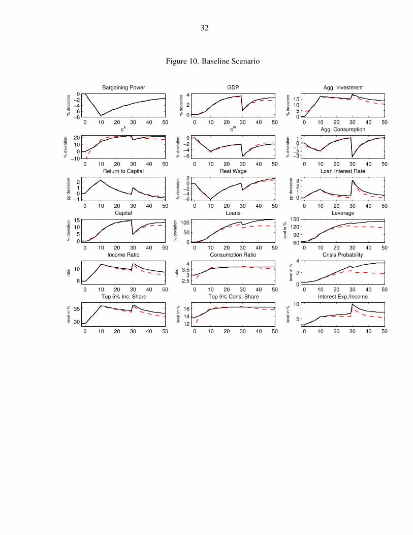
32

Figure 10. Baseline Scenario

0 10 20 30 40 50−8−6−4−2

0Bargaining Power

% d

evia

tion

0 10 20 30 40 50

0

2

4

GDP

% d

evia

tion

0 10 20 30 40 5005

1015

Agg. Investment

% d

evia

tion

0 10 20 30 40 50−10

0

10

20

ck

% d

evia

tion

0 10 20 30 40 50

−6−4−2

0

cw

% d

evia

tion

0 10 20 30 40 50

−3−2−1

01

Agg. Consumption

% d

evia

tion

0 10 20 30 40 50−1

012

Return to Capital

pp d

evia

tion

0 10 20 30 40 50

−6−4−2

02

Real Wage%

devia

tion

0 10 20 30 40 50

0123

Loan Interest Rate

pp d

evia

tion

0 10 20 30 40 500

5

10

15

Capital

% d

evia

tion

0 10 20 30 40 500

50

100

Loans

% d

evia

tion

0 10 20 30 40 5060

90

120

150Leverage

level in

%

0 10 20 30 40 50

8

10

Income Ratio

ratio

0 10 20 30 40 50

2.53

3.54

Consumption Ratio

ratio

0 10 20 30 40 500

2

4Crisis Probability

level in

%

0 10 20 30 40 50

30

35

Top 5% Inc. Share

level in

%

0 10 20 30 40 50

12

14

16

Top 5% Cons. Share

level in

%

0 10 20 30 40 50

5

10

Interest Exp./Income

level in

%

33

Figure 11. Less Capital Investment

0 10 20 30 40 50−8−6−4−2

0Bargaining Power

% d

evia

tion

0 10 20 30 40 50

0123

GDP

% d

evia

tion

0 10 20 30 40 500

10

20

Agg. Investment

% d

evia

tion

0 10 20 30 40 50

−100

1020

ck

% d

evia

tion

0 10 20 30 40 50

−8−6−4−2

0

cw

% d

evia

tion

0 10 20 30 40 50

−4

−2

0

Agg. Consumption

% d

evia

tion

0 10 20 30 40 50

0123

Return to Capital

pp d

evia

tion

0 10 20 30 40 50

−6−4−2

0

Real Wage%

devia

tion

0 10 20 30 40 50

0

2

4

6Loan Interest Rate

pp d

evia

tion

0 10 20 30 40 50

0

5

10

Capital

% d

evia

tion

0 10 20 30 40 500

50

100

150Loans

% d

evia

tion

0 10 20 30 40 506090

120150180

Leverage

level in

%

0 10 20 30 40 50

8

10

12

Income Ratio

ratio

0 10 20 30 40 50

2.53

3.54

4.5

Consumption Ratio

ratio

0 10 20 30 40 500

3

6

9Crisis Probability

level in

%

0 10 20 30 40 50

30

35

40

Top 5% Inc. Share

level in

%

0 10 20 30 40 50

12141618

Top 5% Cons. Share

level in

%

0 10 20 30 40 50

468

101214

Interest Exp./Income

level in

%

34

Figure 12. Nearly Permanent Change in Bargaining Power

0 10 20 30 40 50−8−6−4−2

0Bargaining Power

% d

evia

tio

n

0 10 20 30 40 50

0123

GDP

% d

evia

tio

n

0 10 20 30 40 5005

1015

Agg. Investment

% d

evia

tio

n

0 10 20 30 40 50

0

10

20

ck

% d

evia

tio

n

0 10 20 30 40 50

−6−4−2

0

cw

% d

evia

tio

n

0 10 20 30 40 50−4

−2

0

Agg. Consumption

% d

evia

tio

n

0 10 20 30 40 50

0

1

2

Return to Capital

pp

de

via

tio

n

0 10 20 30 40 50

−4

−2

0

Real Wage%

de

via

tio

n

0 10 20 30 40 50

0123

Loan Interest Rate

pp

de

via

tio

n

0 10 20 30 40 500

5

10

Capital

% d

evia

tio

n

0 10 20 30 40 500

20406080

Loans

% d

evia

tio

n

0 10 20 30 40 5060

90

120

150Leverage

leve

l in

%

0 10 20 30 40 50

8

10

Income Ratio

ratio

0 10 20 30 40 50

2.53

3.54

Consumption Ratio

ratio

0 10 20 30 40 500

1

2

Default Probability

leve

l in

%

0 10 20 30 40 50

30

35

Top 5% Inc. Share

leve

l in

%

0 10 20 30 40 50

12

14

16

Top 5% Cons. Share

leve

l in

%

0 10 20 30 40 50

4

6

8

Interest Exp./Income

leve

l in

%

35

Figure 13. High Variable instead of Low Fixed Subsistence Consumption

0 10 20 30 40 50−8−6−4−2

0Bargaining Power

% d

evia

tio

n

0 10 20 30 40 50

0

2

4

GDP

% d

evia

tio

n

0 10 20 30 40 500

10

20

Agg. Investment

% d

evia

tio

n

0 10 20 30 40 500

102030

ck and c

k

sub

% d

evia

tio

n

0 10 20 30 40 50−6−4−2

0

cw and c

w

sub

% d

evia

tio

n

0 10 20 30 40 50

−2

0

2

Agg. Consumption

% d

evia

tio

n

0 10 20 30 40 50

−1012

Return to Capital

pp

de

via

tio

n

0 10 20 30 40 50

−6−4−2

02

Real Wage%

de

via

tio

n

0 10 20 30 40 50

0123

Loan Interest Rate

pp

de

via

tio

n

0 10 20 30 40 5005

1015

Capital

% d

evia

tio

n

0 10 20 30 40 500

50

100

150

Loans

% d

evia

tio

n

0 10 20 30 40 506090

120150180

Leverage

leve

l in

%

0 10 20 30 40 50

8

10

12Income Ratio

ratio

0 10 20 30 40 502.5

33.5

44.5

Consumption Ratio

ratio

0 10 20 30 40 500

3

6

9Crisis Probability

leve

l in

%

0 10 20 30 40 50

3032343638

Top 5% Inc. Share

leve

l in

%

0 10 20 30 40 50

141618

Top 5% Cons. Share

leve

l in

%

0 10 20 30 40 50

5

10

Interest Exp./Income

leve

l in

%

36

Figure 14. Orderly Debt Restructuring

0 10 20 30 40 50−8−6−4−2

0Bargaining Power

% d

evia

tio

n

0 10 20 30 40 50

0

2

4

GDP

% d

evia

tio

n

0 10 20 30 40 5005

1015

Agg. Investment

% d

evia

tio

n

0 10 20 30 40 50

0

10

20

ck

% d

evia

tio

n

0 10 20 30 40 50

−4

−2

0

cw

% d

evia

tio

n

0 10 20 30 40 50

−2−1

01

Agg. Consumption

% d

evia

tio

n

0 10 20 30 40 50−1

012

Return to Capital

pp

de

via

tio

n

0 10 20 30 40 50

−6−4−2

02

Real Wage%

de

via

tio

n

0 10 20 30 40 50

0

1

2

Loan Interest Rate

pp

de

via

tio

n

0 10 20 30 40 500

5

10

15

Capital

% d

evia

tio

n

0 10 20 30 40 500

50

100

Loans

% d

evia

tio

n

0 10 20 30 40 5060

90

120

150Leverage

leve

l in

%

0 10 20 30 40 50

8

10

Income Ratio

ratio

0 10 20 30 40 50

3

4

Consumption Ratio

ratio

0 10 20 30 40 500

2

Crisis Probability

leve

l in

%

0 10 20 30 40 50

30

35

Top 5% Inc. Share

leve

l in

%

0 10 20 30 40 50

1314151617

Top 5% Cons. Share

leve

l in

%

0 10 20 30 40 50

4

6

Interest Exp./Income

leve

l in

%

37

Figure 15. Restoration of Workers’ Bargaining Power

0 10 20 30 40 50−8−6−4−2

0

Bargaining Power

% d

evia

tion

0 10 20 30 40 50

0

2

4

GDP

% d

evia

tion

0 10 20 30 40 5005

1015

Agg. Investment

% d

evia

tion

0 10 20 30 40 50−10

0

10

20

ck

% d

evia

tion

0 10 20 30 40 50

−4

−2

0

cw

% d

evia

tion

0 10 20 30 40 50

−2

0

2

Agg. Consumption

% d

evia

tion

0 10 20 30 40 50

−1012

Return to Capital

pp d

evia

tion

0 10 20 30 40 50−6−4−2

024

Real Wage%

devia

tion

0 10 20 30 40 50

−1

0

1

Loan Interest Rate

pp d

evia

tion

0 10 20 30 40 500

5

10

15

Capital

% d

evia

tion

0 10 20 30 40 500

50

100

Loans

% d

evia

tion

0 10 20 30 40 5060

90

120

150Leverage

level in

%

0 10 20 30 40 50

8

10

Income Ratio

ratio

0 10 20 30 40 50

2.53

3.54

Consumption Ratio

ratio

0 10 20 30 40 500

2

4Crisis Probability

level in

%

0 10 20 30 40 50

30

35

Top 5% Inc. Share

level in

%

0 10 20 30 40 50

12

14

16

Top 5% Cons. Share

level in

%

0 10 20 30 40 50

4

6

Interest Exp./Incomele

vel in

%