Industrial Structure and Financial Capital Flows∗

Keyu Jin

This Draft: December 20, 2008

JOB MARKET PAPER

Abstract

Factor-proportions trade and financial asset trade are both integral parts of globalization, yetlittle has been studied on their interplay. In a framework that integrates these two paradigmsof trade, a new force driving international capital flows emerges: capital tends to flow towardscountries that become more specialized in capital-intensive industries (a composition effect).This force competes with the “neoclassical force” which channels capital towards the locationwhere it is more scarce, in response to shocks such as globalization, country-specific labor forceor labor productivity shocks. If the composition effect dominates, capital flows away from thecountry hit by the positive shock—“a flow reversal”—and asset prices rise globally rather thanlocally. Two implications arise: rich countries’ current account deficits may be a consequence oftheir shifting towards capital-intensive industries; young and fast growing developing countriesmay help sustain asset prices in an aging industrialized world. Predictions of the current accountand specialization patterns are shown to be consistent with the data.

JEL Classification: F21, F32, F41

Key Words: Globalization, factor-proportions trade, specific-factors, capital flows, currentaccount, asset prices, demographics.∗I would like to thank Kenneth Rogoff for his continual guidance and support. I am grateful to Robert Barro,

Emmanuel Farhi and Gita Gopinath for their invaluable advice. Professors Pol Antras, John Campbell, RichardCooper, Arnaud Costinot, Elhanan Helpman, Nathan Nunn, and Harvard International Economics Workshop andMacroeconomics workshop participants offered helpful comments. I am grateful to Kai Guo, Oleg Itskhoki, KarthikKalyanaraman, Jean Lee, Dan Sacks, and Florent Segonne for his knowledge and support. I thank the NBER Agingand Health fellowship for financial support.

1

1 Introduction

Commodity trade and financial capital flows have both played primal roles in the process of glob-alization, yet there has been little focus on how they interact. A key insight of the neoclassicaltrade theory is that factor endowments form a basis for trade, and countries tend to specialize inindustries that require intensive use of their abundant factor. While specialization patterns are wellunderstood, much less is known about how they affect financial capital flows. The simple notionthat the capital-intensity of a country’s export and production structure may be interrelated withits demand for global financial capital suggests that goods trade and capital flows be analyzedjointly. Yet the convention has been to keep them largely separate in the literatures of interna-tional trade and international macroeconomics. This paper demonstrates that their interaction canbecome crucial, and sheds light on widely-debated issues of global imbalances and asset prices. Inparticular, trade and specialization may cause financial capital to flow from developing countriesto industrialized countries, and lead to a global comovement in investment and asset prices.

In investigating how factor-endowment-based trade and financial asset trade interact, this paperdevelops a framework that integrates these two paradigms of trade. With only basic ingredients,new results emerge and are often surprising. Accompanying the shift in the composition of coun-tries’ production and export structure towards sectors that intensively use their abundant factor isa change in the relative demand and supply of capital. Countries that become more specialized incapital-intensive goods see a concurrent rise in their demand for capital relative to their domesticsupply, and those that become more specialized in labor-intensive sectors see the opposite. A newdriving force of international capital flows thus emerges: financial capital tends to flow towardscountries more specialized in capital-intensive industries (a composition effect). Simultaneouslypresent is the standard, “neoclassical effect” (a slight abuse of terminology) that channels capitaltowards the location where the effective capital-labor ratio is lower. These two forces can becomecompeting, and the direction of international capital flows and the behavior of asset prices areultimately determined by which of the two effects dominates.

A framework that allows for the interplay between factor-proportions trade and financial capitalflows therefore potentially changes the way we think about the macroeconomic impact of certainglobal shocks. Indeed, two pronounced international developments of the past few decades havebeen the rapid trade and financial integration of developed and developing countries, and theirvastly uneven growth in the effective labor force. Faster population growth in developing coun-tries, including the massive rural migration of Chinese workers to the productive urban economy,1

combined with faster labor productivity growth in developing countries,2 contributed to a rapid1 Freeman (2004) estimates that higher population growth in developing countries, and the integration of China,

India, and ex-Soviet bloc increased the labor force in developing countries from 680 million workers in 1990 (beforethe integration of these countries) to 2.23 billion workers in 2000, of which these countries contributed 1.38 billion.This is referred to as the “Great Doubling” of the world labor force.

2Herd and Dougherty (2007) estimates that India’s labor productivity grew by 4.36% over the period 1990-99,and 3.76% over 2000-05. In China, labor productivity grew by 8.66% over 1990-99, and 7.67% over 1999-2005. Theseestimates are consistent with those provided by numerous other studies.

2

increase in the size of the effective labor force in emerging markets.How does faster labor and productivity growth in emerging markets affect world capital flows

and asset prices? According to the one-sector neoclassical model, the emerging South, with a per-manently higher effective labor force, offers higher investment opportunities and should experiencea net capital inflow (the “neoclassical” effect). Yet this relies on the assumption that countriescannot engage in commodity trade, an assumption which is no longer innocuous when countries’comparative advantage are fundamentally altered. That factor proportions is a strong determinantof trade has been most recently, further demonstrated by Romalis (2004), which finds that coun-tries tend to capture larger shares of world production and trade of commodities that require moreintensive use of their abundant factors, and that countries that rapidly accumulate a factor seetheir production and export structures systematically shift towards industries that intensively usethat factor.

Thus, relying on the premise that factor endowment differences form a basis for world trade, anintegrated framework of trade and capital flows can make opposite predictions from the standardmodel. When South becomes relatively more labor abundant and consequently more specializedin labor-intensive goods, its demand for capital rises by less than it would have otherwise in theone-sector case. So while on the one hand, the neoclassical force exerts its impact by drawingcapital away from North to South (where the capital-labor ratio is lower), this force is offset by thecomposition effect, which reduces South’s demand for capital and tends to draw capital towardsNorth. If sectors are sufficiently different so that specialization patterns are pronounced enough,the composition effect dominates, causing a “reverse capital flow”(from South to North); invest-ment comoves across countries, and asset prices rise globally rather than just locally in South. Theprediction, thus, of the emerging periphery running a current account surplus and the industrializedcore running a deficit is more consistent with the data than that of the standard model in whichthe neoclassical effect is the only impetus to capital flows and predicts just the opposite.

The framework developed in this paper provides a rich setting for analyzing a host of widely-discussed issues, delivering new results and certain policy implications. One important predictionis that even if two countries have the same returns to capital prior to opening up their economies,net capital flows are not necessarily precluded once they integrate. A rich country which features ahigher total factor productivity, and therefore a higher capital-labor ratio, exports capital-intensivegoods when opening up to trade. Insofar as countries’ industrial structures change, the composi-tion effect causes rich countries to experience a net capital inflow. Further, the timing of tradeand financial liberalization have different implications for developing countries. While simultaneousliberalization may lead to a capital outflow in South, and an asset price drop, trade liberalizationwithout financial liberalization will prevent such an outflow and lead to an asset price boom.

Beyond its predictions for global imbalances, the framework can also shed light on the widely-debated “asset meltdown hypothesis”. While some believe that the “age wave” hitting industrializedcountries will precipitate a large drop in asset prices as post-war baby boomers start selling assetsfor retirement consumption to a smaller young cohort, the predictions of the framework suggest

3

that the fast-growing and young developing countries can potentially emerge as a remedy. Higherdemand for industrialized countries’ assets from developing countries, as industrial countries be-come more specialized in capital-intensive sectors, will help sustain their asset prices despite theimminent reduction of their labor force. Yet, allowing for the trade channel of adjustment is key.

The framework developed in this paper is a stochastic, two country, Diamond-version overlap-ping generations model with production and capital accumulation, based on the closed-economy,one-good framework in Abel (2003)3. I incorporate multiple sectors that differ in factor intensityto capture factor-endowment trade and allow for financial capital to flow across borders. Thekey difference between this model and a dynamic Hecksher-Ohlin model is the existence of capitaladjustment costs, which endogenously determine the price of capital, and also serve to pin downthe capital stock.4 Despite the numerous features that are embedded in this model, it remains tobe highly tractable, and the new underlying mechanisms are made transparent through either thesemi-closed form or full closed-form solutions obtained in the various cases.

In this integrated framework, the standard neoclassical case becomes only one of two specialcases. When there is a single sector, or when there are multiple sectors but feature no differencesin factor intensities, only the neoclassical effect is present. A second special case, in which the mostlabor-intensive sector uses only labor as an input to production, isolates the composition effectand illustrates a scenario in which factor price equalization leads investment and asset prices toalways comove across countries. The more general case is one in which the neoclassical effect andthe composition effect coexist and primitive parameters determine the relative strength of the two.The last two cases are analyzed separately and brought into sharp contrast to the first.

The main difference between this economy and the majority of either one-good or two-goodstochastic growth models of large open economies (Backus, Kehoe and Kydland (1992), (1994)), isthe assumption of factor-intensity differences across sectors, intended to capture factor-endowmenttrade. The overlapping generations structure featured in the model is analytically convenient al-though not essential. In contrast to two-sector models that do feature factor-proportions trade,such as Ventura (1997), Atkeson and Kehoe (2002), among others, the main difference is that thismodel does not make the assumption that capital needs to stay within borders (that trade is bal-anced).

In spirit, this paper is closer to a few recent papers that also highlight the interaction betweentrade and capital flows, such as Cunat and Maffezzoli (2004), Ju and Wei (2006), and Antras andCaballero (2007). The main point of this paper, in contrast to the others, is that specializationpatterns alone can alter the nature of financial flows.5 Finally, on explaining global imbalances, in

3Abel (2003) develops a closed-economy, one-sector overlapping-generations model with capital adjustment coststo analyze the effect of a baby boom on stock prices and capital accumulation.

4In a Hecksher-Ohlin world with factor price equalization, capital earns the same returns everywhere and can belocated anywhere. Adjustment costs serve to temporarily break FPE and pin down the path of capital.

5 Cunat and Maffezzoli (2004) examine the business cycle properties generated by a multi-sector stochastic twocountry growth model and show that its predictions of the trade balance and terms of trade are more consistentwith empirical facts than in the one-sector model. This paper differs from theirs both in terms of the formalizationof the model and in terms of purpose. In this model, closed-form and semi-closed form solutions are obtainable,explicitly demonstrating the countervailing forces of the neoclassical effect and the composition effect in shaping

4

particular the net flow of capital from South to North, this paper proposes an alternative view high-lighting the importance of trade and specialization, in contrast to others works, such as Caballero,Farhi, and Gourinchas (2008) and Mendoza, Quadrini, and Rios-Rull (2007), that put financialheterogeneity between the two regions at center stage.

The rest of the paper is organized as follows. The multiple-sector framework is described inSection 2. A special case that isolates the composition effect and gives rise to a closed-form solutioncharacterizing the evolution of capital and the price of capital is presented in Section 3. Section 4presents numerical results of the general case in which the composition effect and the neoclassicaleffect coexist, and discusses the conditions under which the composition effect dominates. Addi-tional implications of the framework are taken up in Section 5. Section 6 provides some supportiveempirical evidence on the relationship between specialization and the current account deficit, andSection 7 concludes.

2 The Model Description

Consider a world with two countries, a Home (H) and a Foreign (F ), each characterized by anoverlapping generations economy in which consumers live for two periods. The countries producethe same type of intermediate goods i = 1...m, which are traded freely and costlessly, and areconveniently indexed by their capital intensity, α1 < α2... < αi... < αm. Intermediate goods arecombined to produce a final good, which is used for consumption and investment. Preferencesand production technologies are assumed to have the same structure and parameter values acrosscountries. However, the technologies differ in two aspects: in each country, the labor input consistsonly of domestic labor, and intermediate-goods producing firms are subject to country-specific pro-ductivity and labor force shocks. Henceforward, j denotes countries and i denotes sectors.

2.1 Demographics, preferences and technologies

In each period t, the world economy experiences one of finitely many events st. Denote st =(s0, ..., st) the history of events up through and including period t. The probability at date 0 of anyparticular history st is given by π(st). In the beginning of period t, N j(st) young workers arrivein country j. They inelastically supply one unit of labor in youth, and none when old in the nextperiod. The measure of young consumers, N j(st), is assumed to follow a geometric random walk:

lnN j(st) = lnN j(st−1) + εjN (st)

international capital flows and asset prices. This paper also focuses on shocks that change countries’ comparativeadvantage, and links it to current debates on global imbalances. Ju and Wei(2006) highlight the interaction betweenlabor market rigidities and trade as an impetus to capital flows, while Antras and Caballero (2007) highlight theinteraction between financial heterogeneity and trade. In terms of its formalization, this framework differs from bothof the paper in that the present setting is a stochastic general-equilibrium global model that jointly determines andquantifies the full path of capital, asset prices, and global imbalances.

5

where εN (st) represents a random labor force growth rate which is iid. A high εjN (st) represents alabor force boom.

Each consumer in country j admits preferences of the form

u(cj(st)) =

(cj(st)

)1−ρ1− ρ

where cj(st) denotes the consumption by a consumer in j. Intermediate goods are aggregated by aconstant elasticity of substitution, θ, to form a unit of consumption good and a unit of investmentgood. For any consumer in j,

cj(st) =[ m∑i=1

γ1θi c

ji (s

t)θ−1θ

] θθ−1

where∑

i γi = 1. cji (st) denotes the consumption demand of a j consumer for good i.

Perfectly-competitive firms use domestic labor, supplied by the young consumers, and capitalto produce an intermediate good i in country j:

Y ji (st) = Kj

i (st−1)αi

(Aj(st)N j

i (st))1−αi

(1)

where 0 < αi < 1 for any i. Kji (s

t) is j’s aggregate capital stock in sector i, and N ji (st) is its

aggregate input of labor employed in sector i, at st. Aj(st) represents the country-specific laborproductivity, and follows

lnAj(st) = lnAj(st−1) + εjA(st)

where the growth rate of labor productivity, εjA(st), is iid and is independent of εjN (st), a randomlabor force growth rate.

The capital used in producing good i is augmented by investment goods, Ii(st), and currentcapital stock. The law of motion for capital stock in i is given by Kj

i (st) = G(Kj

i (st−1), Ijt (st))

where Iji (st) is the aggregate investment in sector i in country j at st. G(Kji (s

t), Iji (st)) is linearlyhomogeneous in Kj

i (st) and Iji (st), and there are convex adjustment costs, which satisfy d2Gj

d2Iji (st)< 0.

Following Abel (2003), I take a log-linear specification of G(Kji (s

t), Iji (st)):

Kji (s

t) = a(Iji (st)

)φ (Kji (s

t−1))1−φ

, (2)

6

where 0 6 φ 6 1.6 The purpose of this assumption is to derive analytical solutions for the equilib-rium price and quantity of capital. 7

2.2 Consumers

In the first period, a young consumer in the Home country inelastically supplies one unit of la-bor and earns the competitive wage wh(st), which is used for consumption chy(st), for purchasingstate-contingent securities, bh(st+1), at the corresponding state-contingent price Q(st+1), and forpurchasing capital. Let kh,ji (st) be the amount of capital that a young consumer in Home buys insector i from country j, at a price qji (s

t) per unit, at the end of period t to be carried into periodt+ 1. A Home young consumer’s budget constraint is therefore:

chy(st) = wh(st)−∑j=h,f

m∑i=1

qji (st)kh,ji (st)−

∑st+1|st

Q(st+1)bh(st+1). (3)

Assume that consumers do not have bequest motives, and therefore consume all available resourceswhen they are old. The budget constraint for a Home’s old consumer is

cho (st+1) =∑j=h,f

m∑i=1

Rji (st+1)qji (s

t)kh,ji (st) + bh(st+1) (4)

where Rji (st+1) is the rate of return on capital earned in sector i in country j.

A consumer in Home maximize its lifetime utility of consumption

U = u(cjy(s

t))

+ β∑st+1|st

π(st+1)u(cjo(s

t+1))

where β denotes the discount factor, cjy(st) denotes the consumption of a young consumer in j inperiod t, and cjo(st+1) denotes the consumption by an old consumer in j in period t+ 1.8 A similarset of equations hold for consumers in Foreign.

6As shown in Abel (2003), if φ = 1 and a = 1, the capital accumulation equation becomes the one in the neo-classical growth model with complete depreciation in each period; if φ = 0 and a = 1, this becomes the case of theLucas-tree asset pricing model in which the capital stock is constant.

7In comparing the log-linear model with a standard capital adjustment technology:

Ki(st) = (1− δ)Ki(s

t−1) + Ii(st)− b

2(Ii(s

t)

Ki(st−1)− δ)2Ki(s

t−1),

it can be shown that the two models are equivalent up to the second order if and only if a = φ−φ, δ = φ, b = 1−φφ.

8The first order condition of the consumer’s problem is Q(st+1|st) = βπ(st+1|st)uc(cjo(st+1))/uc(cjy(st)). The

Euler equation associated with any asset i in any country j is uc(cjy(st)) = β

∑st+1|st π(st+1)uc(c

jo(s

t+1))Rji (st+1)

where uc(st) denotes the derivative of the utility function with respect to consumption.

7

2.3 Firms

Firms are perfectly competitive, and choose inputs Kji (s

t), N ji (st), and investment Iji (st) to solve

max∞∑t=0

∑st

Q(st)[pi(st)Yji (st)− wji (s

t)N ji (st)− Iji (st)]

subject to 1 and 2, where pi(st) is the international price of good i, since the law of one price appliesto the freely-traded intermediate goods. wji (s

t) is the real wage paid in sector i in country j at st.The price of capital, qji (s

t), is given by the first order condition for Iji (st). It is the price ofacquiring one unit of capital in sector i and country j (in terms of the consumption good) at theend of period t to be carried into the the next period. This price is the amount that Iji (st) needs

to be increased to increase Kji (s

t) by one unit, that is,(dKj

i (st)/dIji (st)

)−1. This implies that

qji (st) =

1aφ

(Iji (st)

Kji (st−1)

)1−φ

. (5)

If 0 < φ < 1, then qjit is increasing in the investment-capital ratio, Iji (st)/Kji (s

t), of any sector i.In a perfectly-competitive environment, factors are paid their marginal products. Capital in

any sector i in any country j, is productive both in the intermediate goods technology and alsoin contributing to lowering adjustment costs next period. The total rate of return to capital istherefore the sum of capital’s marginal product in the intermediate goods technology, multiplied bythe price of the intermediate good, and its marginal contribution to lowering adjustment costs nextperiod—discounted by the price at which a unit of capital was purchased last period, qji (s

t−1). Thefirst order condition with respect to Kj

i (st), for any i in j, in conjunction to the optimal conditions

of the consumer’s problem defines the rate of return9

Rji (st) =

αipi(s

t)Y ji (st)

Kji (s

t−1)+ 1−φ

φIji (s

t)

Kji (s

t−1)

qji (st−1). (6)

Labor earns its marginal product. The wage rate per unit of labor is given by the first ordercondition with respect to Ni(st):

wji (st) = (1− αi)pi(st)

Y ji (st)

N ji (st)

. (7)

9The first order condition of the firm’s problem with respect to Kji (st) is

1 =∑st+1

Q(st+1|st)(pi(s

t)dY ji (st+1)

dKji (st)

+dIji (st+1)

dKji (st)

)/

(dIji (st)

dKji (st−1)

),

which, combined with the first order conditions from the consumer’s problem given in Footnote 8 yields Eq. 6.

8

2.4 Market Clearing

The intermediate goods markets clear when global demand of any good i equals its global supply:

Y gi (st) =

∑j=h,f

cji (st) +

∑j=h,f

m∑k=1

Ijki(st), (8)

for all i = 1...m. Superscripts g will henceforward represent global variables. cjt (st) is j’s consump-

tion demand of good i, and Ijki(st) is its investment demand of good i in each sector k.10

Domestic labor markets clear when

m∑i=1

N ji (st) = N j(st)

for all j. And market clearing for state-contingent securities require that, for every st,

bh(st) + bf (st) = 0.

The law of one price implies that consumers in each country face the same international pricespi, for all i, which, in conjunction to the assumption of identical preferences across countries, implythat both region’s aggregate price index is equalized. The price index that corresponds to CESpreferences is

P =[ m∑i=1

γip1−θi

] 11−θ

. (9)

P is normalized to 1. The relative price of any two intermediate goods i and k is determined bythe relative world supply of the two goods:11

pi(st)pk(st)

=(γiγk

Y gk (st)Y gi (st)

) 1θ

. (10)

2.5 Equilibrium

The competitive equilibrium of the world economy consists of a sequence of prices [pi(st), Rji (s

t), wji (st)],

and employment and capital allocations [N ji (st),Kj

i (st)] such that consumers and firms in j opti-

mize and markets clear. In what follows, the semi-closed form solution of the equilibrium relies onthree simplifying assumptions, summarized below:

Assumption 1 Preferences are Cobb-Douglas (θ = 1)

10The demands for consumption and investment goods implied by a CES demand function are cji = γ( piP

)−1θ Cj

and Ijki = γ( piP

)−1θ Ijk, for all st, where P is the domestic price index.

11 Using consumption and investment demands of any i and k, plugging into Eq. 8 yields the relative price of i andk.

9

Assumption 2 Consumers have logarithmic preferences (ρ = 1)

Assumption 3 The capital-adjustment technology is log-linear

Assumptions 2 simplifies the consumption/saving problem so that private saving does not dependon the real rate of return. Without assumption 2, optimal consumption in this two-country in-vestment model cannot be characterized analytically, and therefore neither are optimal investmentand capital. When assumptions of 1 and 3 are combined with assumptions 2, the global aggregateinvestment-output ratio and the global industry-level investment-output ratio are both constants.Relying on these results, capital accumulation in each sector i in any country j, is characterized byone key variable—the present discounted value of the expected future share of output of i produceddomestically. Although no closed-form solution is available in general, the system of equations forma contraction mapping that leads to a simple numerical algorithm, described in Appendix C.2. Afull closed-form solution of the equilibrium exists for a special case, presented in Section 3. Withoutthese assumptions, neither the semi-closed form solution in the general case nor the full closed-formsolution in the special case is possible. In later sections all of these assumptions are relaxed, and itis shown that none are crucial for the main results of interest.

Assuming that consumers have logarithmic utility, the optimal consumption of a young con-sumer in period t is a constant fraction of the present value of lifetime resources, which in thismodel is simply the wage income earned by the young. For notational simplicity, I will hencefor-ward suppress the notation st and denote period t as subscript t. The aggregate consumption ofthe young cohort, Cjyt = N j

t cjyt, is 12

Cjyt =1

1 + βW jt , (11)

where W jt =

∑iw

jitN

jit denotes the aggregate wage in j.

At the world level, consumption of the young is a constant fraction of labor income, which,by the assumption of Cobb-Douglas preferences, occupies a share sl = 1−

∑i αiγi of world GDP,

denoted as Y gt , and Y g

t =∑

i piYgi ,. The result that global investment is a constant fraction of

global output immediately follows:13

Igt = ψslYgt (12)

where ψ = φβ1+β and Igt =

∑j

∑mi=1 I

jt .

To determine investment at the industry level, let Igit = µitIgt so that µit represents the share

12Substituting 4 into 3 and aggregating, and using Eq. 6, and the first order conditions of the consumer’s problemyields Eq. 11.

13Aggregating Eq. 3 across countries gives Cy,gt = W gt −

∑mi=1 q

hitK

Hi,t+1 −

∑mi=1 q

FitK

Fi,t+1, where Kj

i,t+1 =

kH,ji,t+1Nht+1 + kF,ji,t+1N

Ft+1 is the total amount of financial capital claimed by the world on j. Then, setting the

expression for optimal aggregate consumption of the young to the left hand side of the equation, Eq. 11, while usingthe fact that qjitK

ji,t+1 = Ijit/φ from Eq. 5 gives Eq. 12.

10

of industry i’s investment in aggregate investment, and Ihit = ηitIgit so that ηit represents Home’s

share of global investment in sector i. Investment in any sector i, in any country h, f , can thus bewritten as

Ihit = µitηitψslYgt (13)

Ifit = µit(1− ηit)ψslY gt . (14)

It can be shown that

Lemma 1

µit =αiγi∑i αiγi

∀t (15)

Proof. See Appendix C.2.Total global investment in i, Igi , is a constant fraction of global output, and is increasing in itscapital share αi, and the preference for that industry’s good, γi. The reason that industry-specificshocks do not come into play in determining industry-level investment is that the assumption ofCobb-Douglas preferences (Assumption 1) implies that any movements in relative prices are offsetby changes in output, so that nominal output remains unchanged. This eliminates the need forresource allocation across industries.

Deriving the full solution to the economy’s equilibrium amounts to solving for the crucial variableηit, the country-share of investment in sector i. Relying on the three simplifying assumptions (1-3),this share can be written explicitly as,14

ηit = (1− λ)∞∑k=0

λkEt

(Y hi,t+k+1

Y gi,t+k+1

), (16)

where λ =β(1−φ)

1+βsksl

+β(1−φ)

1+β

< 1. Ihit is thus determined by Home’s expected, present-discounted value of

the share of its future output in good i, the discount factor λ depending on the size of adjustmentcosts. In the absence of adjustment costs, φ = 1, future output after date t + 1 does not matter,and investment in sector i is determined by its expected share of output of good i at t + 1. Thehigher the adjustment cost (lower φ), the higher the discount factor λ (λ′(φ) < 0), and the greaterthe desire to smooth investment over time.

Finally, Equations 13, 14, 15, and 16, combined with the evolution of the capital stock, inj = h, f :

Kji,t+1 = aIjit

φKjit

1−φ

14 Using the Euler equation, u′(ct) = Et[βu′(ct+1)Rit+1], and the risk sharing condition,

cyt

cot+1=

cy,gt

co,gt+1

, while

plugging in optimal consumption of the young, from Eq. 11, and the old, given in the Appendix C.2, yields ηit =

(1− λ) + λEt[Y hi,t+1Ygi,t+1

] where λ =β(1−φ)

1+βsksl

+β(1−φ)

1+β

. Iterating forward yields Eq. 16.

11

Investment in Homeα = 0.3 α1 = 0.1, α2 = 0.5

ηi −11.13% −12.46%, −1.4%η −3.24%Y g +10% +6.86%Ih −1.13% +3.62%

Table 1: Impact Effect of an unexpected 20% labor force boom in Foreign; Iht = ηt + Y gt ; γi = 0.5.

together pin down a unique path of capital, and yield the full solution to the equilibrium of thiseconomy.

2.6 An Illustration of the Composition Effect

To see the effect of composition (of production) on a country’s investment demand, write aggregateinvestment at Home as Iht = ηtψslY

gt , where

ηt =m∑i=1

µiηit (17)

represents its weighted average share of global production, with the weights µi = αiγi∑i αiγi

increasingin αi and γi. Evidently, more weight is put on the capital-intensive sectors when determining acountry’s investment share. By contrast, in a one-sector model, since only one good is produced,a positive technology or labor force shock in Foreign causes a large drop in the present-discountedexpected value of Home’s share of global output, and consequently its share of investment. Butwhen there are compositional shifts, less weight is put on the sectors that contract in Home (labor-intensive sectors) and more weight is put on the sectors that expand (capital-intensive sectors ). Inthe end, the weighted average share of investment ηt falls by significantly less than it would havehad in the one-sector case.

To illustrate this point more concretely, Table 1 gives the percentage changes in ηt and Iht

in response to 20% labor force shock abroad for a one sector and a two-sector example. WhileHome’s share of expected production of any good i falls unilaterally (ηi is negative for all i), forthe reason that Foreign’s relative size in the world has increased, this share falls by much morefor the labor-intensive sector than for the capital-intensive sector (−12.46% vs −1.4%). Thus,the weighted-average expected share of future output falls significantly less in the two-sector casecompared to the one-sector case(−3.24% vs. −11.13% ), making the overall change in investmentat Home positive rather than negative (3.62% vs −1.13%).

12

2.7 The Initial Steady State

Assuming that initial capital-labor ratios across countries are not too different so that economiesare within the cone of diversification, countries diversify in production, and conditional FPE holdsin the deterministic steady state. The trading equilibrium yields the same resource allocations andprices as the world’s integrated equilibrium, in which both goods and factors are perfectly mobileinternationally. The equilibrium is one in which a constant fraction of world resources is spent ineach sector:

Ngi =

(1− αi)γisl

Ng

andKgi =

αiγisk

Kg

where Ngi =

∑j N

ji represents effective world labor supply in sector i. In this equilibrium, there is

a multiplicity of steady states, arising from the fact that an infinite number of allocations of capitalacross countries is consistent with factor price equalization (conditional on technology). However,the existence of adjustment costs pins down a unique path of capital, so that given initial conditionsKj

0/Nj0 , the transitional dynamics leads the system to a unique steady state.15 In this economy, con-

ditional FPE does not hold in the transition to the steady state, but is attained only in the long run.

3 The Composition Effect

In general, analytical solutions are not obtainable in the two-country stochastic models with invest-ment and adjustment costs, and analyses are generally restricted to numerical simulations. Whenincorporating multiple sectors with differing factor intensities, the special case in which the mostlabor-intensive sector uses only labor as an input to production effectively shuts off the neoclassicalforce, and isolates the composition channel of adjustment. Consequently, a closed-form solution forthe price and quantity of capital arises. The special case requires the additional assumption that:

Assumption 4 α1 = 0.

With this assumption, the wage in any region j is given by the wage paid in the first sector, wj1t =Ajtp1t. Since intermediate goods’ prices are equalized through trade, conditional wage equalization,whit/w

fit = Aht /A

ft , holds in any period t and state st, despite stochastic shocks. It follows that

khit = kfit (18)

where kjit = Kjit

AjtNjit

is the effective capital-labor ratio in sector i. Labor reallocates across sectors toequalize effective-capital labor ratios in each sector, across countries.

15A more detailed discussion can be found in Cunat and Maffezzoli (2004), which also introduce adjustment coststo pin down the capital stock in a world of FPE. An alternative is to assume that countries start out from autarky(described in Appendix B ), where capital stock at the country-level is pinned down, and the equilibrium is unique.

13

Consider a high εfN,t (labor force boom) or εfA,t (productivity boom) in Foreign. In order toequalize wages across sectors, Foreign expands relatively more the labor-intensive sectors. Therise in the world supply of labor-intensive goods relative to that of capital-intensive goods putsdownward pressure on the relative price of labor intensive goods. For what range of goods doprices fall or rise? It can be shown that

pk ≤ 0 ⇔ αk ≤∑i

αiγi

where pk denotes the percentage change of the price of good k (proof in Appendix B). Prices risesfor sectors with capital shares greater than the weighted average capital share, the weights γi beingthe effective size of the sector.

In response to greater profitability of capital-intensive sectors, Home responds by drawing laborout of the first sector and reallocating it towards capital-intensive sectors. Domestic labor reallo-cation ensures that ki, for all i 6= 1, is equalized across countries in every period. Of course, thisrelies on the condition that both countries produce the most labor-intensive good. Appendix Bshows a sufficient condition for which all goods are produced by both countries. Intuitively, thesize of sector 1 needs to be large enough and the shock small enough so that both countries arerequired to produce the good.

The market share of region j’s production in sector i is pinned down by its share of capitalstock in sector i, since Y j

it/Ygit = Kj

it/Kgit follows from Eq. 18. It is thus the case that Home’s share

of investment in i, ηit, using Eq. 16, becomes

ηit = λ∞∑k=0

(1− λ)kEt[Khi,t+k+1

Kgi,t+k+1

]. (19)

Proposition 1 With Assumptions 1− 4, ηit = Khi0

Kgi0.

The share of Home’s investment in any industry i, ηit, is a constant and is equal to its initial shareof world capital in that sector.Proof. To prove that ηit = Kh

i0

Kgi0

, guess that Khit

Kgit

= ηit, and show that ηit = ηi0 is a solution to acontraction mapping, consisting of Eq. 19 and the Cobb-Douglas production technologies, Eq. 1and 2. By the contraction mapping theorem, it is the unique solution. Appendix B provides detailsto the full proof.

The intuition of this result is that commodity trade (of goods with different factor intensities)brings about the equalization of sectoral capital-labor ratios across countries at all points in time,through industrial rearrangement. This ensures that the marginal product of capital from theproduction side, αipik

j,αi−1i , is equalized at all times. Therefore, in investing the marginal unit of

savings, Foreign allocates it to both countries, and in such a way that marginal adjustment costspaid in sector i and country j, proportion to Iji

Kji

, are equalized. The standard neoclassical forcethat tends to equalize sectoral capital-labor ratios is effectively shut down, isolating the compo-

14

sition channel of adjustment. Despite adjustment costs, factor price equalization is attained oneperiod after the shock. The investment ratio across regions in each sector will depend on theirinitial capital stock ratio in that sector, making this economy path dependent.

3.1 Aggregate Savings and Investment

Summing investment, given by Eq. 13, across sectors, and using Proposition 1, country j’s aggregateinvestment at t becomes

Ijt =∑i

µiηji0ψslY

gt , (20)

where ψ = φβ/(1 + β), sl = 1 −∑

i αiγi and µi is given by Lemma 1. A high εjA,t or εjN,t whichraises world GDP raises investment globally, and in such a way that more investment is allocatedto country j that has a higher initial, weighted-average capital-intensity,

∑i µiη

ji0. In this special

case with international trade linkages, investment comoves.A graphical exposition offers some basic intuition to these results. Relying on the closed-form

solution, one can write j′s domestic output to world output, Y jt /Y

gt , denoted as f , as a function

of its relative capital-labor ratio t, κjt = kjt /kgt :

16

f(κjt ) =

(sl

κjt+ 1

)∑i

µiηji0 (21)

Aggregate savings-to-output ratio in j can be written as

S(κjt ) = ψ

1− 1slκjt

+ 1

. (22)

Analogously, the investment-to-output ratio in j can be written as

I(κjt ) =ψslslκjt

+ 1. (23)

The I(κjt ) and S(κjt ) curves cross at the point at which κjt = 1, where the the capital-labor ratiosare equalized across countries, or in other words, where no country has a comparative advantageover another.

16 pitYjit can be conveniently expressed as γiY

gtYjit

Ygit

. Since Y jit/Ygit = Kj

it/Kgit = N j

it/Ngit = ηji0 , and domestic GDP

is Y jt =∑i piY

ji =

∑i 6=1 γiη

ji0 + γ1

˜Nj1

Ng1

. Wage equalization across sectors in j, (1 − αi)pitY jit/Njit = AjtN

j1t ∀ i 6= 1,

implies N jit = (1 − αi)γi/γ1η

ji0N

g1 where i 6= 1. j’s domestic to world GDP ratio, Y jt /Y

gt , can be expressed as in

Eq. 21.

15

The I(κjt ) and S(κjt ) schedules are graphed in the first panel of Figure 1. Greater comparativeadvantage in labor (to the left of κt = 1) causes greater specialization in labor-intensive goods,which raises the relative share of output allocated to wage income. Since savings derives fromwage income in this model, the saving-to-output curve is therefore downward sloping. On the otherhand, greater specialization in labor-intensive goods reduces the share of output that is neededfor investment, and the investment-to-output curve is upward sloping. The difference between thecurves represents j’s current account as a share of GDP. The two curves intersect at the pointwhere countries’ capital-labor ratio is equalized, the point at which domestic savings is just enoughfor domestic investment, and no net capital flows needs to occur between countries. A positiveshock that reduces j’s relative capital-labor ratio at t leads to a compositional shift that causes itssupply of savings to rise by more than its investment demand, the difference of which shows up asa current account surplus.

Similarly, one can graph the savings and investment curves in the one sector model. In this case,the investment-GDP curve is downward sloping, as drawn in the second panel of Figure 1. Thereason is that by the neoclassical force, a permanent labor force boom in Foreign that reduces itscapital-labor ratio induces higher investment so that capital can scale up with labor. On the otherhand, the savings rate is a constant, a result of assuming logarithmic utility and a Cobb-Douglasproduction function. In contrast to the multi-sector model, j moves into greater current accountdeficit as its capital-labor ratio falls.

These two figures depict the savings-investment relationship when the composition effect andthe neoclassical effect are each respectively isolated. The striking difference is the slope of theinvestment demand, from negative in the multi-sector case to positive in the one-sector case. In thegeneral case, where both composition and neoclassical effects coexist, the investment-output curvelies somewhere in between—and becomes positively sloped when the composition effect is strongerand negatively sloped when the neoclassical effect is stronger. The condition for which one effectdominates the other is demonstrated in Section 4.3.

3.2 The Price and Quantity of Capital

The evolution of the effective aggregate capital-labor ratio is characterized by:

kjt+1 = Θ

(∑i

µiηji0

)φsle−(εjN,t+1+εjA,t+1)

(Ngt

N jt

)φsl(kt

j)1−φsl , (24)

where Θ is a constant.17 This implies the following propositions:

Proposition 2 ( Path Dependence) The evolution of the kjt depends on j’s initial weighted-averagecapital-intensity,

∑i µiη

ji0; the higher the initial weighted-average capital intensity in j, the higher

the effective capital-labor ratio in j at every point of the transitional path.

17Θ = a(ψsl/sk∏γγii (αiγi)

αiγi [(1− αi)γi]1−αiγi)φ

16

0.6 0.7 0.8 0.9 1 1.1 1.2 1.3 1.40.05

0.06

0.07

0.08

0.09

0.1

0.11Multiple Sector Case (Composition Effect Only)

Relative Capital Labor Ratio

S/YI/Y

CA/Y

0.6 0.7 0.8 0.9 1 1.1 1.2 1.3 1.4

0.14

0.145

0.15

0.155

Relative Capital Labor Ratio

One Sector Model

I/YS/Y

-CA/Y

Figure 1: Savings/GDP and Investment/GDP ratio as a function of κjt , kj

kg. The first panel shows the

multiple sector case, based on closed-form solutions. It assumes that α1 = 0, α2 = 0.3, α3 = 0.5, α4 = 0.9,γi = 0.25 for all i. The second panel shows the simulated results of the one sector case, based on Eq. 16when i = 1; α1 = 0.3, β = 0.7 and φ = 0.5.

17

The country with the higher initial capital intensity commands lower marginal adjustment costpaid on investment in that country, and thus occupies a higher share of world investment.

The price of capital is defined as the weighted average of the price of capital in each sectori 6= 1, the weights being the capital share of that industry in total capital stock of region j, Kj

i

Kj .The logarithm of the price of capital in sector i in j evolves according to:

lnqjit = [1− φsl]lnqji,t−1 + (1− φ)sl(lnNgt − lnN

gt−1)− lnΘi,

where Θi is a sector-specific constant. This leads to the following proposition:

Proposition 3 (Price of capital) qjt in any region j and any sector i, where i 6= 1, is an increasingfunction of a positive labor force or labor productivity shock if φ < 1, and follows a stationaryprocess if 0 < φ < 1.

Proposition 3 provides conditions under which the price of capital in both countries rises in responseto a labor force boom or a positive shock to labor productivity in any region. If φ = 1, the caseof complete depreciation, the price of capital is constant and equal to 1/a. In the more interestingcase where φ < 1, the price of capital at Home rises in response to a high εfN,t or εfA,t. If capital canbe accumulated (φ > 0), then the price of capital is stationary. However, if capital stock is fixedover time (φ = 0), as in the Lucas-tree model, the price of capital is non-stationary. By contrast,in the one sector case, the price of capital tends to fall at Home when φ < 1, as investment flowsabroad to take advantage of higher investment opportunities.

Proposition 4 Country j’s stock market-capitalization to domestic GDP ratio at t,∑i6=1 q

jitK

ji,t+1

Y jt

is increasing in j’s relative capital-labor ratio, kjt /kgt .

Using qjitKji,t+1 = (1/φ)Ijit, this result immediately follows from Eq. 2318.

Corollary 5 The ratio of sector i’s stock market-capitalization to domestic GDP, in any countryj, is increasing in αi, γi, ηi0.

Proposition 4 indicates that the smaller the comparative advantage in labor of Home, the higherits aggregate stock-market value to GDP ratio. This result is consistent with the sharp rise in thevalue of stocks in the 1990’s in the U.S. On the other hand, Corollary 5 says that the stock marketvalue of sector i depends on its effective capital-intensity, αiγi, and the expected share of globaloutput it produces, ηi0.

Aggregate investment is the economic channel through which a labor force boom or a produc-tivity shock affects the price of capital, and trade in goods with different factor intensities is theconduit through which aggregate savings can be allocated globally rather than locally. A laborforce boom or a labor productivity boom in period t leads to a high aggregate wage income, which

18In the one-sector, closed-economy framework of Abel (2003), the stock market-capitalization to domestic GDPratio is a constant in the long run.

18

is accrued to Foreign’s young consumers, who are the savers in the economy. As Foreign becomesrelatively more labor-abundant, it shifts its industrial structure towards more labor-intensive sec-tors. Consequently, Foreign’s supply of savings rises by more than its demand for investment, thedifference of which is exported to Home. The high level of aggregate investment relative to thecapital stock in t, which is predetermined, drives up the price of capital along the upward-slopingsupply curve of capital, Eq. 5, in both countries.

4 The Competing Forces of the Neoclassical and Composition Ef-

fects

The previous special case which isolates the composition effect leads to factor price equalizationafter one period. Investment and asset prices always comove across countries. However, FPE nolonger holds in a case where all sectors use both capital and labor as inputs to technology except inthe steady state. The neoclassical and the composition effect coexist and are competing, and thequestion of which effect dominates becomes a numerical issue. I show that when factor intensitiesare sufficiently different in a multiple-sector world, the composition effect outweighs the neoclassicaleffect, and the previous qualitative results on asset prices and financial flows are preserved.

4.1 General Capital Adjustment Function and Parameter Values

For quantitative purposes, the drawback of the log-linear capital adjustment function is that depre-ciation and adjustment costs, both of which are captured by the parameter φ, cannot be separated.However, a second-order Taylor approximation shows that the log-linear model and a standardcapital-adjustment model

Ki,t+1 = (1− δ)Kit + Iit −b

2(IitKit− δ)2Kit

are equivalent if φ = δ, b = (1− φ)/φ, and a = φ−φ. Henceforward, the general capital adjustmentmodel is used in the quantitative exercises.

A realistic calibration of a two-period model clearly has its limitations. If one period is inter-preted to be 20 years, then adjustment costs are inevitably going to be very small, if paid evenlyover time.19 Capital adjustment costs are widely used in international RBC models but there is noconsensus on the calibration strategy to parameterize them.20 The strategy adopted in this modelis to take a standard adjustment cost parameter value, b = 1, based on an annual frequency, and

19Assuming the existence of some adjustment costs, albeit small in size, is necessary since zero adjustment costswould automatically lead us to the case of indeterminacy of capital stock at the country level.

20 For example, Baxter and Crucini (1993) calibrated the elasticity of investment relative to Tobin’s q to matchinvestment variability in industrial countries. Chari, Kehoe, and McGrattan (2000) calibrated the parameter to matchthe relative variability of consumption to output. Kehoe and Perri (2002) targeted the variability of investment.

19

compute the amount of capital adjustment that takes place over twenty years. Then, the parameterb is chosen, in a twenty year period model, so that the same amount of capital adjustment takesplace as in the annual frequency model over the same time horizon. Admittedly, no calibrationtechnique of the adjustment cost parameters will be entirely satisfactory, although it can be shownthat the qualitative results are insensitive to the size of the adjustment costs, and that the quanti-tative results are driven to a much larger extent by factor intensity differences than by adjustmentcosts. Section 4.3 reports sensitivity analysis. The discount factor β is set to 0.45 to match theinitial steady-state annual real interest rate of 4%.

The baseline model takes benchmark case where the of Cobb-Douglas preferences, i.e. θ = 1.In this case, γi’s are equal to the share of sector i in the world’s total value added, in an integratedequilibrium. Estimates of factor intensity shares and γi’s are provided in Cunat and Maffezoli(2004). Using OECD Annual National Accounts Detailed Table, they aggregate the value of 28sectors across 24 OECD countries, and calculate the share of each sector in total OECD valueadded. γi’s are then calibrated to match these observed shares. Since 1 − αi is just the sector’slabor share in value added, one can use data on compensations of employees to compute the sectorallabor share. Assuming that production technologies are identical across countries, the labor shareacross sectors is taken from U.S. data.21 In aggregating the 28 sectors into two large sectors, I rankthe sectors by their capital intensity and assume that the first 14 sectors are labor-intensive, andthe second half capital intensive. γ is then chosen such that γ =

∑14i=1 γi. α1 and α2 are calibrated

to match the weighted mean of the capital share of the 28 sectors, sk =∑28

i=1 γiαi = 0.36, andthe weighted variance,

∑i γi(αi − sk)2, which is 0.04 as measured from the 28-sectors data. The

resulting parametrization is γ = 0.61, α1 = 0.11, and α2 = 0.52.Although the key results of interest pertain to symmetric countries as well as asymmetric coun-

tries, the exercise is done for countries that are meant to mimic a developing and a developedcountry. Therefore, the two countries differ in initial capital-labor ratios and labor productivity.While higher initial capital-labor ratio in North increases the amount of investment flows fromSouth (the path dependence result), lower initial labor productivity in South reduces the extent ofits capacity to save and therefore the amount of investment that flows to North. Initial capital-laborratios for each country are taken from Hall and Jones (1999). As a whole, developed countries’capital-labor ratio is about 6 times as large as that of developing countries in 1988. TFP in Northis chosen to normalize per capita income to 1, and TFP in South is chosen to match South’s incomeper capita being one seventh of that of North in 1988.

4.2 Impulse Response

The experiment I consider is one in which the effective labor force in South unexpectedly doublespermanently. The impact effect on goods and factor prices are shown analytically in Appendix C.2.

21Internationally comparable estimates for all sectors and all countries are available only for 1995 and 1996. Theyassume that factor intensities have not changed significantly over time.

20

Since capital is fixed for one period, in order to equalize wages, South allocates a greater fractionof labor to the labor-intensive sector. The higher world supply of labor-intensive goods causes therelative price of labor goods p1 to fall, and the price of capital goods p2 to rise. In response to thegreater profitability in the capital-intensive sector, North shifts resources there, and the return tocapital rises in the capital-intensive sector, which is North’s export sector, and falls in its importcompeting sector. The real wage is depressed in South as a result of a greater supply of labor. InNorth, the real wage rises with respect to purchases of the import good but falls with respect topurchases of the export good, so that the overall effect is ambiguous. For reasonable parametervalues, it tends to fall in North.

Figures 2 displays the response of other variables. The vertical axis represents the levels of eachvariable normalized by its initial value. The horizontal axis represents generations. Investmentcomoves as South partly finances North’s investment in the capital-intensive sector. The rise ininvestment in North and the fall in its savings (as a result of declining wages) lead to a currentaccount deficit. The increase in investment initially generates a trade deficit in North, followed bya permanent trade surplus as it pays capital gains and interest income abroad.

The increase in investment in both countries causes the aggregate price of capital to be bidup globally. However, the price of capital behaves differently across sectors in each country: whilethe price of capital rises in both sectors in South, the price of capital falls in the labor-intensiveindustry in North as a result of the downsizing of that sector.

Figure 3 juxtaposes the response of North in the one-sector and two-sector case, and bringsthe two cases in sharp contrast. In the benchmark one-sector case, North’s GDP, investment andprice of capital fall as capital flows from North to South to take advantage of the latter’s higherreturns. Intuitively, since only one capital-to-labor ratio is consistent with the steady state in theone-sector case, an increase in labor in South implies an equivalent scaling up of capital in Southin the long run. Since capital accumulation takes time, in the presence of adjustment costs, Northinitially finances some of South’s investment, and runs a current account surplus. It runs a tradedeficit to finance higher consumption in North, while South runs an initial trade surplus. In thelong run, trade is balanced between the two countries.

4.3 When does the composition effect dominate?

When the neoclassical effect and the composition effect are competing, the result that investmentand asset price comove, while capital flows are “reversed” relies on the composition effect out-weighing the neoclassical effect. The composition effect is strong when specialization patterns arepronounced, and the extent of specialization depends on factor intensity differences across sectors.In the limit where factor intensities converge to the same level, the multi-sector model yields qual-itatively similar results to a one-sector model, and the neoclassical effect is isolated. As factorintensities become more disparate, the composition effect becomes stronger. So how different dofactor intensities have to be in order for the composition effect to prevail?

21

In a simple two-sector case where the only difference across sectors come from the capital share,i.e. the case where γ = 0.5, a simple statistic to gauge the extent of specialization is the factorintensity ratio α2/α1. The first graph in Figure 4 shows the results of the response of North’sinvestment, at the time of the shock, for various values of the factor-intensity ratio in the m = 2case. The inflection point is the crucial ratio of 1.4, above which North’s investment rises and be-low which North’s investment falls . This cutoff ratio is naturally also the point where the changein the price of capital turns from negative to positive, and where the current account turns fromsurplus to deficit. This shows that as factor intensities become more similar, the neoclassical effectdominates, causing investment to fall in North, and the qualitative results converge to those of theone-sector case. The more different are factor intensities, the more pronounced are specializationpatterns, and the stronger is the composition effect. The relative strength of the composition effectand the neoclassical effect matters not only qualitatively but also quantitatively.

What is an analogous simple statistic for the multi-sector case? The reasonable measure of thedispersion of factor intensities in this case is the weighted variance of αi, with weights γi capturingthe effective size of the sector:

w.v =m∑i=1

(αi − sk)2γi

Estimated from the OECD data with 28 sectors, the weighted mean of capital intensity,∑

i αiγi, is0.36, and the weighted variance is 0.04. The experiment that holds fixed the weighted mean whileincreasing the weighted variance shows that North’s investment again rises with the dispersion offactor intensities. Figure 4 plots the regression line of Home’s investment response when simulatinga model with five sectors.22 The correlation is strongly positive. As the weighted variance of sectorsincreases, Home’s investment rises. The inflection point is around a weighted variance of 0.02 whenthe weighted mean is held fixed at 0.36.

Other parametersAdjustment costs change the quantitative response of asset prices and the current account althoughnot their qualitative predictions. Table 3 shows that increasing adjustment costs causes a higherjump in the price of capital at Home, and induces a smaller current account deficit as the amountof desired investment falls. Qualitatively, the price of capital always rises and the current accountalways falls for Home, so long as factor intensities are sufficiently different. Moreover, the magni-tudes of the current account’s responses are to a much larger extent governed by factor intensitydifferences than by the change in the size of the adjustment costs, as can be seen from the variousinteractions between the values of b and α2/α1.

The impact of adjustment costs on the current account is different in the one-sector case. Whilehigher adjustment costs lead to a smaller current account deficit in North in the two-sector case,it leads to a greater current account surplus in North in the one sector case. The reason is that

22There is no unique correspondence between North’s investment level and the weighted variance, since there isone extra degree of freedom in choosing parameters to satisfy a constant weighted mean and weighted variance. Forthis reason, only a linear regression line of the simulated responses is plotted.

22

rather than bearing all of the cost of adjusting capital, South imports capital from North, who ispaid a higher price of capital in return. Further, the results are not very sensitive to the coefficientof relative risk aversion and the elasticity of substitution. None of these parameters, except for thefactor intensity ratio, matter qualitatively for the main result at hand. The current account pat-tern of North running a deficit and South a surplus, along with investment comovement and assetprice comovement are solely governed by the dispersion of capital intensities, which determines thestrength of the composition effect.

5 Applications and Discussions

The integrated framework developed in this paper is able to deliver a number of new predictionsfor a host of issues. Although a thorough treatment of various applications to the framework isbeyond the scope of this paper, this section points to a few important predictions that stand instark contrast to the standard one-sector models.

5.1 Globalization and the “Lucas Paradox” Revisited

As originally pointed out by Lucas (1990), large differences in capital-labor ratios may not implyvast differences in the marginal product of capital, as poor countries also have lower endowments offactors complementary with physical capital, such as human capital and total factor productivity.This has been attributed to be a main reason explaining why very little capital flows from rich topoor countries.

Over the past decade, a more puzzling phenomenon has emerged: not only has there been verylittle capital flowing from rich to poor countries, but flows have been entirely reversed. Developingcountries are running a current account surplus, while developed countries are running a currentaccount deficit. If MPK’s are indeed similar, this pattern cannot be reconciled in a standardneoclassical model without appealing to some type of friction, of which a most recent popularone has become financial heterogeneity.23 Yet, the standard assumption that inherently differenttrading economies can only produce the same, single good (with rich countries only producing moreof it) is unreasonable in this context. In the data, developing and developed have comparativeadvantages in the production of different goods. Romalis (2004) shows that as an aggregate whole,industrial countries tend to capture higher market shares of U.S. imports in more capital-intensiveindustries.24

It seems thus natural to incorporate the possibility of commodity trade when analyzing theimpact of globalization on capital flows and asset prices. The following analysis shows that allowingfor the interaction between goods trade and asset trade can become crucial.

Assume that two countries are initially in autarky. The difference between the industrialized23 See Caballero, Gourinchas, and Farhi (2008) and Mendoza, Quadrini, Rios-Rull (2007), Antras and Caballero

(2007).24More precisely, the study shows that every 1 percentage point increase in the capital intensity leads to to a

0.5-percentage point rise in industrial countries’ market share of U.S. imports.

23

North (country n) and the emerging South (country s) is that North features a higher total factorproductivity (TFP). The autarkic equilibrium (described in Appendix A) is one in which goodsand factor prices are determined by their respective aggregate capital-labor ratio:

pj,autk ∝ (Kj

N j)∑i αiγi−αk (25)

wj,aut ∝ Aj(Kj

N j)∑i αiγi (26)

Rj,autk ∝ Aj(Kj

N j)∑i αiγi−1 (27)

In the initial steady state, returns are pinned down by preferences, which are equalized acrosscountries. Thus, a higher TFP in North than in South, An > As, implies a higher capital-laborratio in North (shown in Appendix A). According to Eq. 32, capital-abundant North features alower relative price of capital-intensive goods: (pkpi )n,aut < (pkpi )s,aut for any good k > i. Since theinternational price of good i once countries open up to trade is just the weighted average of theautarky prices in the two regions, North will see an increase in the price of all goods i such thatpn,auti < ps,auti , or in other words, all goods i ≥ k such that

αk ≥∑i

αiγi,

and South will see an increase in the price of goods i < k.25 As a consequence, North becomesmore specialized in capital-intensive goods and South in labor-intensive goods.

Trade liberalization causes wages to rise in South and to fall in North, in the m = 2 case (ana-lyzed in Appendix C.1). Since wage income accrues to the young consumers, who are the savers inthe economy, aggregate savings rises in South. Insofar as countries shift their industrial structurein response of trade liberalization, South sees a reduction in its supply of capital relative to itsdemand for capital. In this case, the neoclassical force remains dormant (since initial returns wereequalized), and simultaneous trade and financial liberalization therefore leads to a unambiguousnet capital inflow in North, by the composition effect.

Numerical results in the m = 2 case are displayed in Figure 5. TFP differences are chosenso that North’s capital-labor ratio is initially taken to be about six times that of South. Otherparameters are taken to be the same as before, provided in Table 2. The experiment assumes thatcountries initially start from autarky, and globalization is introduced as a permanent unanticipatedregime change of both trade and financial liberalization. The overall impact is a rise in the aggre-gate price of capital in North and a fall in South. The capital-intensive sector contracts sharplyin South, causing a large drop in the price of capital in that sector. The price of capital riseshowever, in the labor-intensive sector where investment demand is high. The opposite occurs inNorth. Since North’s savings falls at the same time that its investment rises, it runs a large currentaccount deficit to GDP ratio.

25 If (KN

)n > (KN

)s, pnx < psx iff∑αiγi − αk > 0.

24

The implication is that we cannot use the similarity in MPK’s across countries to infer that therewill be little capital movements across regions when these economies open up. The reason is that animportant channel of adjustment is through trade, which can cause the respective marginal productof capital to diverge as a consequence of industrial restructuring. Yet, while trade liberalizationand financial liberalization are both integral parts of globalization, the timing of liberalization havedifferent implications on developing countries. While simultaneous liberalization may lead to a cap-ital outflow in South, and an asset price drop, trade liberalization without financial liberalizationwill prevent such an outflow and lead to an asset price boom. The reason is that a rise in wageincome in South, as a consequence of trade liberalization, raises aggregate savings. Since aggregatesavings need to contemporaneously equal aggregate investment in the context of financial autarky,higher aggregate investment drives up the price of capital.

5.2 Demographic Divergence and Asset Prices

This framework can also be applied to address the looming “age wave” of industrialized countriesthat has garnered much attention from policy makers and academics alike. Just as some believethat the post-war baby boom and its flow of private savings had fueled the stock market and sentstock prices soaring in the past two decades, others fear that the imminent “age wave” that ishitting the industrialized countries will precipitate an “asset meltdown” as baby boomers startselling their large quantities of stocks for retirement consumption to a much smaller group of youngcohort. Abel (2003), among others, shows that a baby boom causes an initial increase in the priceof capital, followed by a fall.

Yet, the opposite demographic trend is occurring in developing countries. Figure 6 shows thatdemographic trends have diverged between industrialized countries and emerging markets sincethe mid-1980s, and is likely to continue for the next few decades. According to Jeremy Siegel, inpopular press, the far younger, and rapidly growing developing world can emerge as a solution tothe “age wave crisis”, as they procure the purchasing power needed to purchase assets from thedeveloped world. Closer scrutiny of this argument under the discipline of a neoclassical frameworksuggests that this is untenable. If anything, faster labor force or productivity growth in emergingmarket would only cause their savings to stay mostly locally, where marginal product of capitaland investment demand is high. It will likely generate further drops in asset prices in industri-alized countries if investment takes place abroad. Yet, in a world where comparative advantagedetermines the structure of trade, and financial capital moves freely, higher labor force and/orlabor productivity growth in emerging markets can potentially help sustain asset prices in an agingNorth.

Two caveats are in order. The first is that these results rely on the premise that demographicdifferences translate into differences in comparative advantage, and affect specialization patterns.While no existing empirical relationship has been established between demographics factors andthe structure of trade, Section 6 takes a first step in this direction. A second caveat is that one may

25

argue that labor force booms arising from demographic trends are to some extent anticipated. Inreality labor-force booms are neither completely unexpected (demographic trends are predictableup to a certain point) nor completely anticipated (migration, female labor force participation, la-bor force reforms), but lie somewhere in between. Figure 7 shows results from the extreme casein which a labor force boom is perfectly anticipated, and contrasts the predictions of a one-sectorcase and a two-sector case scenario. Initially, before the shock occurs, South starts accumulatingcapital a few periods ahead in expectation of a labor force boom at t = 4, since capital can only begradually accumulated in the presence of adjustment costs. It is achieved through investment flowsfrom North, whose consumers benefit from being paid higher asset prices. North thus initially runsa current account surplus while South runs a deficit, before the shock occurs. However, at the timeof the shock t = 4, aggregate savings in South rises and capital allocation of the additional savingsinvolves sending capital both locally and abroad, since North now specializes in capital-intensivesectors. The overall qualitative result on asset prices and capital flows is maintained in the an-ticipated case, for the periods after the shock, although its quantitative effect is tempered. Thecontrast remains sharp with the one-sector case, whereby the price of capital and investment fallsand mean reverts for North, and the rise in asset prices is entirely accrued to Southern consumers,rather than shared across countries.

5.3 Protectionism

The previous results rely on an environment where goods market and financial markets are bothperfectly integrated. However, either trade autarky or financial autarky can lead to vastly differentpredictions for the current account and asset prices. Consider the following results:

Result 1: If countries can engage in free goods trade but financial capital is not allowed to flowacross borders (i.e. if trade has to be balanced), then a positive labor force or productivity shock inSouth will cause the price of capital to rise in South, and to fall in North.

This result comes from the fact that aggregate savings must equal aggregate domestic investmentin the absence of international movement of financial capital. As North shifts to capital-intensivesectors, the reduced demand for domestic labor can cause wages to fall in North (shown in Ap-pendix C.1). Since aggregate savings derive from wage income, aggregate investment falls and putsdownward pressure on the price of capital in North. This implies that protectionist policies inNorth can exacerbate the consequences of its shrinking labor force.

Result 2: If financial capital can flow across borders but countries cannot engage in free tradein goods, South’s price of capital will rise while North’s price of capital will fall as a consequenceof a positive labor force or productivity shock in South.

26

With the trade channel entirely shut off, a positive labor force or productivity shock in Southwill cause no changes in the patterns of specialization, and hence no impetus for capital flows in-duced by changes in industrial structure. Capital will flow from North to South to capture higherinvestment opportunities, leading to a decline in the price of capital in North.

6 Empirical Implications and Evidence

A central prediction of the model is that countries which have become more specialized in capital-intensive industries experience greater demand for financial capital and thus run a greater currentaccount deficit. Since no studies have yet examined the empirical relationship between the currentaccount and the capital-intensity of a country’s export, this segment of the paper serves as astarting point. The theory does not provide a closed-form solution relating the current accountand specialization patterns, and therefore I perform a reduced-form regression.

A requisite variable is a measure of a country’s capital intensity of exports. To construct thismeasure, I borrow a notion of “revealed comparative advantage” (RCA) often adopted in the tradeliterature. Most recently, Romalis (2004) uses this measure to examine the relationship betweenfactor proportions and the structure of trade. To do so, he estimates a country-specific coefficientαc from the following regression:

xcz = βc + αc · kz + γc · sz + εcz (28)

xcz is the share that country c commands of U.S. imports in industry z, k and s are the capitalintensity and skill intensity of industry z. αc is thus the percentage point increase in country c’smarket share of z, for each 1-percentage point increase in capital-intensity. Countries can thus beranked according to αc, a “revealed comparative advantage” in capital-intensive sectors.

Factor intensities, k and s, of each industry are calculated using the “NBER ManufacturingIndustry Productivity Database”, which covers 459 industries, until 1996. I assume that factor in-tensities of each industry are the same across countries and thus use the U.S. data as a benchmark.As a result of data availability, I also assume that between the periods of 1996-2006, the factorintensities of industries have not changed. Following Romalis (2004) k is measured as 1 less theshare of total compensation in value added. s is measured as the share of nonproduction workersin total employment in each industry. U.S. imports (data described in the appendix) are classifiedby detailed commodity and country of origin.

To examine the “RCA” for developing and developed countries as a whole, regression 28 is firstperformed for South, defined to be countries with per capita GDP at PPP of not more than 50percent of the U.S. level in each period.26 South’s market share is calculated as xsz =

∑c∈South xcz

26 North comprises of Australia, Austria, Belgium, Canada, Denmark, Spain, Finland, France, Greece, HongKong, Ireland, Iceland, Israel, Italy, Japan, Netherlands, Norway, New Zealand, Singapore, Sweden, and the UnitedKingdom.

27

for each industry z. The periods in consideration are 1989, 1993, 1998, 2002, and 2006. Table 4reports the results for South over time. South’s market share falls significantly with the capital in-tensity of the industry. Each 1-percentage point increase in capital intensity is estimated to reduceSouth’s market share by 0.75 percent in 2006. Between the period 1989-2006, South’s “RCA” incapital-intensity fell from −0.47 to −0.75, with the largest drop occurring between 1989-93. Theopening up of China and India over this period may have contributed to the fall in capital intensityof developing countries, as these countries were largely labor abundant. The model performs wellfor the aggregate South and therefore for the aggregate North.

6.1 Empirical Relationship between Specialization and the Current Account

Using αc, the ”RCA” in capital-intensive goods, I proceed to examine whether there is a systematicrelationship between a country’s capital-intensity of exports and the current account in a panelregression model. The regression specification considered is27

CAct = α+ β1 · αct + γ′Zct + uct (29)

where CAct is the current account to GDP ratio, αct is country c’s coefficient on capital intensity,28

Zt is a vector of controls, and uct is a disturbance term. The sample period covers 1989, 1993, 1998,2002 and 2006. Control variables are taken from the standard literature, provided in both Gruberand Kamin (2005) and Chinn and Prasad (2003).29 These include per capita income, GDP growthrate, demographic variables (population growth and the share of working age population to totalpopulation), and openness.

Panel regression estimates are presented in Table 5. The first column shows the OLS estimatesof β1 in a regression that pools all country/year observations. The estimate obtained from thepooled regression uses all the available variation in αc’s and current accounts. A 1-percentagepoint higher market share of U.S. imports for every 1-percentage point increase in capital inten-sity is associated with a 0.19-percentage point fall in the Current-Account/GDP ratio. To givea sense of the meaning of this magnitude, consider a concrete example. In 2002, India’s coeffi-cient αc was −0.7, and China’s −2.19. Their actual current account/GDP ratio was respectively1.38% and 2.4%. By contrast, Great Britain’s αc was 2.9, and Australia’s was 1.1. Their currentaccount/GDP ratio were respectively −1.56% and −3.7%. The regression results imply that hadIndia attained U.K’s degree of specialization in capital-intensive goods, 25% of the actual differencebetween their CA/GDP ratios is explained by differences in specialization. Similarly, had Chinareached Australia’s degree of specialization, 20% of the actual current account difference between

27I assume that the measurement error arising from estimating αct is uncorrelated with uct.28 It is derived based on normalized shares of import, xcz, where by the the import share in country c in industry

z is divided by the average value of xcz, so as to make αc comparable across countries.29Unlike these papers, I do not include measures for financial crisis, financial deepeness and fiscal balances.

28

the two countries is explained.The OLS estimates, however, omit variables that vary across countries but are constant across

time (such as institutions, macroeconomic environment), and those that are constant across coun-tries but vary across time (such as oil prices). For this reason, fixed-effects panel regressions areperformed. Another reason for using fixed-effect estimation is to separate the between-countryvariation from the within-country variation, which is the focus of the empirical analysis as it mostclosely reflects the central theoretical prediction that countries which become more specialized incapital-intensive industries over time run greater current account deficits. Column (6) reports thecoefficient estimate that use both between-country and within-country variation. The estimatein column (4) uses only the between-country variation, while the estimate in (5) uses only thewithin-country variation. The coefficients are negative and highly significant. The magnitudesof the fixed-effect coefficient and the within coefficient are similar, suggesting that both between-country and within-country variation are important in explaining current account dynamics. Thewithin-regression coefficient suggests that countries that become more capital-intensive over timerun higher current account deficits.

These results are clearly preliminary, and a more thorough empirical analysis of the relation-ship between specialization and the current account needs to take into account the possibility thatcountries’ current account dynamics may vary, and that there may be omitted variables that arecorrelated with the capital-intensity of exports and also affect the current account. For instance,countries with better financial institutions may be net exporters of more capital-intensive goodswhile at the same time being better producers of quality assets, which some believe to have causedthe large current account deficits in the U.S. The extent of the analysis conducted in the paper canonly serve as a starting point, but at the very least, these initial results seem to suggest that thereis a systematic negative relationship between specialization patterns and current account dynamics,one which that has not been examined before, and one which is consistent with the predictions ofthe theoretical framework.

6.2 The Relationship between Demographics and Specialization

The next question I examine is the relationship between demographic factors and specializationpatterns. While there has been little disagreement on whether globalization has engendered tradepatterns largely driven by factor endowment differences between developing and developed coun-tries, little is known about whether demographic factors and their impact on the labor force alsoaffect specialization patterns. To the extent that the most important aspect of demographic change,for the purpose of this analysis, is its impact on the labor force, the demographic variable adoptedis the working age to total population ratio. To examine whether changes in demographic factorsover time affect specialization patterns, I exploit the panel dimension of the data and perform theregression

αct = βc + Sharect + γ′Zct + εct (30)

29

for all countries. Sharect is the ratio of working-age population to total population in country c att.

Table 6 reports the results. Variables that vary across countries but that are constant over timeare clearly important in explaining specialization patterns. The within regression result (column(3)) suggests that a 1-percentage point increase in the share of working-age population over timeis associated with a 0.27-percentage point reduction in the country’s “RCA” in capital-intensiveindustries. The coefficient results are negative and significant, and are robust to the inclusion ofadditional controls, such as per-capita income and population growth. These results suggest thatcountries’ demographic trends may potentially be an important factor in contributing to specializa-tion patterns. Thus, future demographic differences between developing and developed countriesmay cause diverging specialization patterns, and therefore the trade channel of adjustment shouldbe taken into account when analyzing their impact on current account dynamics and global assetprices.

7 Final Remarks

International commodity trade and asset trade are inherently intertwined processes of globalization,yet the workhorse international-macro model has neglected to analyze them jointly. The capital-intensity of a country’s export and production structure affects its demand for financial capital,and financial capital inflows into a country can affect its extent of specialization in capital-intensiveindustries. This interaction is key in determining global allocations of capital and the behavior ofasset prices. A simple and yet more realistic enrichment of the standard model to include multiplesectors thus compels us to reassess the way a variety of shocks impinge on the world economy.

In the framework that I develop, a novel force that coexists with the neoclassical force in shapingglobal capital flows emerges: capital tends to flow towards countries that become more specializedin capital-intensive sectors. This implies that the integration of developing South and industrializedNorth, or faster labor force/productivity growth in the former can lead to capital flows from Southto North. This stands in sharp contrast to the prediction of the standard one-sector model, and isconsistent with the existing global current account patterns.

The interaction between goods trade and asset trade is worthy of further investigation. Forexample, a natural implication of the framework is that trade liberalization and financial asset lib-eralization have differential impact on emerging market’s asset prices. Whereas simultaneous tradeand financial liberalization may cause asset prices to fall in emerging markets, for the reason thatcapital flows towards North where the capital-intensity of production is higher, trade liberalizationalone can cause a rise in asset prices in emerging markets through its positive impact on wages andaggregate savings.

Looking towards the future, emerging markets’ lagging demographic transitions combined withfaster productivity growth can emerge as a potential remedy to the age mismatch of the indus-

30

trialized economies. Higher global demand for North’s assets as it becomes more capital-intensivecan help sustain asset prices despite the imminent reduction of its labor force. Yet this outcomedepends critically on the extent of financial and trade integration of world economies. Impedimentsto the free flow of goods and capital among countries, along with rising protectionism in certainparts of the world, will inevitably curtail the ability to share these shocks on a global level. But ifwe believe that greater interdependence is the direction towards which the world is heading, all themore important is a synthesized framework that takes into account a comprehensive set of forcesthat shape our global economy.

31

References

[1] Abel, A. B. (2003):“The Effects of a Baby Boom on Stock Prices and Capital Accumulationin the Presence of Social Security”, Econometrica,71, 551-578.

[2] Alfaro, L. and E. Hammel (2007):“Capital Flows and Capital Goods”, Journal of InternationalEconomics,72, 128-150.

[3] Amano, A. (1977) :“Specific Factors, Comparative Advantage and International Investment”,Economica, 44, No.174, 131-144.

[4] Antras, P. and R. J. Caballero (2007):“ Trade and Capital Flows: A Financial Frictions Per-spective”, mimeo, 1-37.

[5] Atkeson, A. and P. J. Kehoe (2000):“ Path of Development for Early-and Late-Boomers in aDyanmic Hecksher-Ohlin Model”, Federal Reserve Bank of Minneapolis Staff Report, 256.

[6] Attanasio, O., S. Kitao, and G. Violante(2006): “Global Demographic Trends and SocialSecurity Reform,” Journal of Monetary Economics, 54, 144-198.

[7] Backus, D. K., P. J. Kehoe, and F. E. Kydland (1992):“International Real Business Cycles,”Journal of Political Economy, 100, 745-775.

[8] Borsch-Supan, A., A. Ludwig, J. Winter (2005): “Aging, Pension Reform, and Capital Flows:A Multi-Country Simulation Model”, 1-44.

[9] Caballero, R. J., E. Farhi, P-O. Gourinchas (2008):“ An Equilibrium Model of “Global Imbal-ances” and Low Interest Rates,” The American Economic Review, 98, 358-93.

[10] Barro, R. J., and J. Lee (2000):“International Data on Educational Attainment: Updates andImplications,”CID Working Paper No. 42.

[11] Beaudry, P., F. Collard (2006):“Globalization, Returns to Accumulation and the World Dis-tribution of Output per Worker,” Journal of Monetary Economics, 53(5), 879-909.

[12] Cunat,A. , and M. Maffezzoli (2004):“ Heckscher-Ohlin Business Cycles”, Review of EconomicDynamics, 555-585.

[13] Davis, D. R. , and D. E. Weinstein (2001a):“An Account of Global Factor Trade”, AmericanEconomic Review, 91, 1423-53.

[14] Davis, D. R. , and D. E. Weinstein (2001b):“The Factor Content of Trade”, Handbook ofInternational Trade, E. Kwan Choi and James Harrigan, eds., New York: Blackwell, 2002.

[15] Davis, D. R. , and D. E. Weinstein (2001c):“Do Factor Endowments Matter for North-NorthTrade?”, NBER Working Paper #8516, October 2001.

32

[16] Guscina, A., (2006 ): “Effects of Globalization on Labor’s Share of National Income?”, IMFWorking Paper WP/06/294, December 2006.

[17] Hall, R. E, and C. I. Jones (1999):“Why Do Some Countries Produce So Much More Outputper Worker than Others?”, Quarterly Journal of Economics, 114, 83-116.

[18] Harrison, A. E., (2002):“Has Globalization Eroded Labor’s Share? Some Cross-Country Evi-dence.”, Berkeley, CA: University of California at Berkeley and NBER, mimeo.

[19] Herd, R., and S. Dougherty (2007):“Growth Prospects in China and India Compared”, Euro-pean Journal of Comparative Economics, 4(1), 65-89.

[20] Ju, J. and S. Wei,(2007): “Current Account Adjustment : Some New Theory and Evidence”,NBER Working Paper No. 13388.

[21] Mayer, W., (1974): “Short-run and Long-Run Equilibrium for a Small Open Economy”, Jour-nal of Political Economy, 82(5), 955-67.

[22] Mendoza, E. G., V. Quadrini, J. Rios-Rull(2007): “Financial Integration, Financial Deepness,and Global Imbalances”, NBER Working Paper No.12909.

[23] Mundell, R., (1957): “International Trade and Factor Mobility”, The American EconomicReview, 47, 321-335.

[24] Mussa, M., (1978): “Dynamic Adjustment in the Hecksher-Ohlin-Samuelson Model”, Journalof Political Economy, 86(5), 775-91.

[25] Neary, J. P., (1978): “Short-Run Capital Specificity and the Pure Theory of InternationalTrade”, Economic Journal, 88, 488-510.

[26] Romalis, J. (2004):“Factor Proportions and the Structure of Commodity trade”, The AmericanEconomic Review, March, 67-97.

[27] Ventura, J. (1997):“Growth and Interdependence”, The Quarterly Journal of Economics, 112,57-84.

33

A Appendix: Initial Equilibrium

The Open Economy: The following results assume θ = 1. If countries diversify in production,factor prices are equalized in the steady state, which is just the integrated equilibrium. A constantfraction of world resources is spent in each sector:

Ngi =

γi(1− αi)sl

Ng

andKgi =

γiαisk

Kg,

where sk =∑

i αiγi, and sl = 1−sk. In the open-economy steady state, goods price and factor pricesare independent of domestic factor endowments and determined entirely by world endowments:

pipj∝(Kg

Ng

)αj−αiwhere Ng

i = AnNni +AsN s

i represents world effective labor in sector i.Factor prices are given by:

w ∝ A(Kg

Ng

)∑αiγi

R ∝(Kg

Ng

)∑αiγi−1

.

Returns are pinned down by preferences in the steady state. From the Euler equation,

R =CgoβCgy

=1 + β

βsl(∑i

αiγi +1− φφ

ψsl), (31)

in the log-utility case, ρ = 1. Global consumption of the old, Cgo , and global consumption of theyoung, Cgy , are derived in C.2.

Autarky: Assume that North and South differ by total factor productivity, As < An, and areinitially in autarky. The autarkic equilibrium is one in which the equalization of factor prices acrosssectors, together with the goods market clearing condition, give rise to the result that a constantfraction of resources is spent on each sector:

Ni =γi(1− αi)

slN

andKi =

γiαisk

K

34

and where the absolute price of any good k is determined by:30

pk ∝(K

N

)∑i αiγi−αk

(32)

Wages and returns can be expressed as:31

w ∝ A(K

N

)∑i αiγi

R ∝ A(K

N

)∑i αiγi−1

,

which, in the steady state, is pinned down by preferences, the same as in the integrate equilibrium,Eq. 31. Since preferences are assumed to be the same across countries, An > As implies that thecapital-labor ratio is higher in North:

(KN

)n>(KN

)s. From 32, it is thus the case that pnk < psk⇔∑

i αiγi − αk < 0. International goods prices after opening up the economies to trade will be aweighted average of the autarky prices in each country, and therefore trade liberalization raises allprices of goods k in North such that αk >

∑i αiγi.

B The Closed-Form Solution

Proof of Proposition 1:Proof. Guess that Kh

it

Kgit

= ηit, and using Ki,t+1 = aIφitK1−φit , Ihit

Ifit= ηit

(1−ηit) by construction,

Y hi,t+1

Y gi,t+1

=Khi,t+1

Kgi,t+1

=1

1 +Kfi,t+1

Khi,t+1

=1

1 + (1−ηit)φ

ηφit

(Kfit)

1−φ

(Khit)

1−φ

= ηit

This shows that if Khit

Kgit

= ηit, then we naturally haveKhi,t+1

Kgi,t+1

= ηit. By induction,Khi,t+m+1

Kgi,t+m+1

= ηi,t+m =

ηi,t+m−1 = ... = ηi0, for any k ≥ 0, so thatY hi,t+m+1

Y gi,t+m+1= ηi0 ∀k ≥ 0.

30Using the price index 1 =∏i pγii and the relative price formula pi

pj= γi

γj

YjYi

for any i and j, we find

the absolute price for any good k, pk =∏i ( γk

γi

YiYk

)γi . This leads to Eq. 32, where more precisely, pk =

(sl/sk)sk−αk∏i(γk/γi)

−γi(αiγi)αiγi [(1− αi)γi](1−αi)γi .

31More precisely, w = Msl−slsk

−skαkαk (1−αk)1−αkA(K

N)sk , and R = M(sk/sl)

sk−1αkαk (1−αk)1−αkA(K

N)sk−1.

35

This implies that:

ηit = λ∞∑m=0

(1− λ)kEt[Khi,t+m+1

Kgi,t+m+1

]

= λ∞∑m=0

(1− λ)mEt[ηi0],

= ηi0,

which proves that the guess ηit = ηi0 is a solution that satisfies the contraction mapping.Next I derive results supplementing the main results in Section 3. In a model which imposes

assumptions (i) − (v), wage equalization across sectors and conditional wage equalization acrosscountries give the result that capital-effective labor ratios in each sector i is equalized across coun-tries, and global labor allocated to each sector i is a constant fraction of the world labor force, asis labor in all sectors i 6= 1 in j:

khi = kfi (33)

Nhi

Ngi

= ηi (34)

Ngi

Ng=

(1− αi)γi1−

∑i αiγi

= νi (35)

(36)

Prices: Using the fact that γipi = 0 (the definition of the price index) and pi−pj = αiNi−αjNj ,(the wage equalization condition), the percentage change in the price of good k can be written as

pk = αkNgk −

∑i

αiγiNi

Since Ngi is a constant fraction of world labor, it must be that

pk > 0⇔ αk >∑i

αiγi

Wages:

wf = pk − αiˆNfk

= −∑i

αiγiˆNi

= −∑i

αiγiˆNg < 0

36

Since wh

wf= Ah

Af, wages also fall at Home.

A Sufficient condition for diversification in production: The assumption of Cobb-Douglas demand preferences implies that the output of good 1, Y g

1′, rises in response to a labor

force boom or a TFP shock, since Y gi′ = γi(Y

gi )′ for all i, where “′” denotes variables after the

shock. This implies that

Nh′1 +Nf ′

1 > Nh1 +Nf

1 . (37)

Since wages fall at Home, from above, we know that

(i) ∆kij< 0 ∀i 6= 1 (38)

(ii) ∆Nh1 < 0, ∆Nf

1 > 0, ∆N ji < 0 ∀i 6= 1 (39)

For non-specialization to occur, it must be that both countries produce the most labor-intensivegood, good 1, so that:

N s′1 −N s

1 < ε (40)

Nn′1 > 0 (41)

From Eq. 37,

Nf ′1 −N

f1 < ε⇔ Nh

1 −Nh′1 < Nf ′

1 −Nf1 < ε (42)

⇒ Nh′1 > N1 − ε (43)

A sufficient condition for which Nh′1 > 0, and hence, diversification in production, is therefore

ε < Nh1

C Derivation of the General Model and Numerical Method

This section derives the two-sector general case and provides the computational method. Theanalog for the multiple-sector case follows directly.

C.1 Factor and Goods Prices

A high εfN,t: The impact effect of a labor force boom in Foreign on factor and goods prices canbe analyzed analytically in the case of θ = 1 in the two-sector case. Denoting hat variables as

37

percentage changes, we have, in any country j:

wj1 = p1 − α1Nj1 (44)

wj2 = p2 − α2Nj2 (45)

Rj1 = p1 + (1− α1)N j1 (46)

Rj2 = p2 + (1− α2)(N j2 ), (47)

where we assume that εjA,t = 0 for all j. Capital is predetermined and therefore a fixed factorin period t. Since p2 > 0 and p1 > 0 following a high a labor force boom in Foreign, only oneconfiguration of the change in goods and factor prices is possible:

Rh2 > p2 > wh?0 > p1 > R1 (48)

Rf1 > Rf2 > p2 > 0 > p1 > wf . (49)

To determine wage behavior at home, first observe that wage equalization within a country at anypoint in time implies w1 = w2, which, in conjunction to the condition that γp1 + (1− γ)p2 = 0,implies that w2 = (γ − 1)α2(N2) − γα1N1. The condition that determines whether wages rise orfall in Home amounts to:

wht < 0⇔Nh

1,t−1

Nh2,t−1

<γ

1− γα1

α2(50)

For standard parameter values, wages tend to fall at Home while it falls unambiguously in Foreign.

A Globalization Shock: A similar analysis shows that in response to a globalization shock:

Rh2 > p2 > 0 > wh1 , wh2 > p1 > Rh1 (51)

Rf1 > p1 > ws1, ws2 > 0 > p2 > Rs2 (52)

where wages falls unambiguously in North, since condition 50 is satisfied in the closed-economyequilibrium, where Nh

1

Nh2

= γ(1−α1)(1−γ)(1−α2) (from Appendix A).

C.2 Model Derivation

Let the relative price of good 1 and good 2 be pt = p1tp2t

, and xt be the fraction of labor allocated tosector 1 at Home. For notational convenience, home country subscripts are ommitted, and foreigncountry variables are denoted as subscript f . The wage equalization conditions are:{

p1tp2t

(1−α1)Y1t

(1−α2)Y2t= xt

(1−xt)

pt(1−α1)Y1t,f

(1−α2)Y2t,f= xtf

(1−xt,f ) .

38

Using Eq. 1 and using the expression for the relative price pt = γ1−γ

Y g2tY g1t

, these two equations can berewritten as:

xα1t

(1− xt)α2=

Nft

Nt

α1−α2Kα11t K

α22t,f

Kα11t,fK

α22t

xα1ft

(1− xt)α2(53)

γ(1− α1)(1− xt)

1 +N

1−α1t K

α11t,f

N1−α1t K

α11t

x(1−α1)ft

x(1−α1)t

=(1− γ)(1− α2)xt

1 +N

1−α2ft K

α22t,f

N1−α2ht K

α22t

(1−xft)(1−α2)

(1−xt)(1−α2)

(54)

At each point in time t, given Kit, Kif,t, At, Aft, xt, xt,f are uniquely pinned down by these twoequations.

Summing Eq. 4 across countries, and using (Ig1t + Ig2t)/φ = β1+β [p1t(1 − α1)Y g

1t + p2t(1 − α2)Y g2t],

denoted as Sgt , the global consumption of the old can be expressed

Cgo,t+1 = p1,t+1α1Yg1,t+1 + p2,t+1α2Y

g2,t+1 +

1− φφ

(Ig1,t+1 + Ig2,t+1),

= [pt+1α1Y

g1,t+1 + α2Y

g2,t+1

pt+1(1− α1)Y g1t+1 + (1− α2)Y g

2t+1

+β(1− φ)

1 + β](p1,t+1(1− α1)Y g

1t+1 + p2,t+1(1− α2)Y g2t+1).

Substituting this into the Euler equations u′(ct) = Et[u′(ct+1)Rji,t+1], while letting Ig1tφ = µtS

gt ,

I1tφ = µtηtS

gt , and I2t

φ = (1− µt)κtSgt , we have

µt = Et[

pt+1α1Yg1,t+1

pt+1(1−α1)Yg1t+1+(1−α2)Y

g2t+1

+β(1−φ)

1+βµt+1

pt+1α1Yg1,t+1+α2Y

g2,t+1

pt+1(1−α1)Yg1t+1+(1−α2)Y

g2t+1

+β(1−φ)

1+β

],

µtηt = Et[

pt+1α1Y1,t+1

pt+1(1−α1)Yg1t+1+(1−α2)Y

g2t+1

+β(1−φ)

1+βµt+1ηt+1

pt+1α1Yg1,t+1+α2Y

g2,t+1

pt+1(1−α1)Yg1t+1+(1−α2)Y

g2t+1

+β(1−φ)

1+β

],

(1− µt)κt = Et[

α2Y2,t+1

pt+1(1−α1)Yg1t+1+(1−α2)Y

g2t+1

+β(1−φ)

1+β(1−µt+1)κt+1

pt+1α1Yg1,t+1+α2Y

g2,t+1

pt+1(1−α1)Yg1t+1+(1−α2)Y

g2t+1

+β(1−φ)

1+β

]

39

Substituting in pt = γ1−γ

Y g2tY g1t

yields

µt =α1γ

(1−α1)γ+(1−α2)(1−γ)α1γ+α2(1−γ)

(1−α1)γ+(1−α2)(1−γ) + β(1−φ)1+β

+β(1−φ)

1+β

α1γ+α2(1−γ)(1−α1)γ+(1−α2)(1−γ) + β(1−φ)

1+β

Et[µt+1],

= λ1 + λ3Et[µt+1].

µtηt =α1γ

(1−α1)γ+(1−α2)(1−γ)α1γ+α2(1−γ)

(1−α1)γ+(1−α2)(1−γ) + β(1−φ)1+β

Et[Y1t+1

Y g1t+1

] +β(1−φ)

1+β

α1γ+α2(1−γ)(1−α1)γ+(1−α2)(1−γ) + β(1−φ)

1+β

Et[µt+1ηt+1]

= λ1Et[Y1t+1

Y g1t+1

] + λ3Et[µt+1ηt+1]

(1− µt)κt =α2(1−γ)

(1−α1)γ+(1−α2)(1−γ)α1γ+α2(1−γ)

(1−α1)γ+(1−α2)(1−γ) + β(1−φ)1+β

Et[Y2t+1

Y g2t+1

] +β(1−φ)

1+β

α1γ+α2(1−γ)(1−α1)γ+(1−α2)(1−γ) + β(1−φ)

1+β

Et[(1− µt+1)κt+1]

= λ2Et[Y2t+1

Y g2t+1

] + λ3Et[(1− µt+1)κt+1]

The first equation implies that µt is a constant µ = λ11−λ3

= λ1λ1+λ2

= α1γα1γ+α2(1−γ) , since λ1+λ2+λ3 =

1. The two remaining equations become: ηt = (1− λ3)Et[Y1t+1

Y g1t+1] + λ3Et[ηt+1]

κt = (1− λ3)Et[Y2t+1

Y g2t+1] + λ3Et[κt+1].

Iterating forward, ηt = (1− λ3)∑∞

k=0 λk3Et[

Y1t+k+1

Y g1t+k+1]

κt = (1− λ3)∑∞

k=0 λk3Et[

Y2t+k+1

Y g2t+k+1]

C.3 Computational Method

In the two-sector case, solving the model amounts to finding the set of paths η, κ,K,Kf such that:

for all time step t

ηt = (1− λ3)Et[Y1t+1

Y g1t+1] + λ3Et[ηt+1]

κt = (1− λ3)Et[Y2t+1

Y g2t+1] + λ3Et[κt+1]

K1,t+1 = a(φµηtSgt )φK1t1− φ

K2,t+1 = a(φ(1− µ)κtSgt )φK1−φ

1t

K1f,t+1 = a(φµ(1− ηt)Sgt )(φK1−φ1f,t

K2f,t+1 = a(φ(1− µ)(1− κt)Sgt )φK1−φ2f,t

, (55)

with Sgt = β1+β [p1t(1 − α1)Y g

1t + p2t(1 − α2)Y g2t] and where sector-dependant productivities Yit+1

and Yit+1,f are computed from sector-dependant capitals Kit and Kit,f using the wage equalization

40

conditions: xα1t

(1−xt)α2= Nft

Nht

α1−α2 Kα11t K

α22t,f

Kα11t,fK

α22t

xα1t,f

(1−xt,f )α2

γ(1−α1)(1−xt)

1+N

1−α1ft

Kα11t,f

N1−α1ht

Kα11t

x(1−α1)tf

x(1−α1)t

= (1−γ)(1−α2)xt

1+N

1−α2ft

Kα22t,f

N1−α2ht

Kα22t

(1−xft)(1−α2)

(1−xt)(1−α2)

. (56)

For every time step t, we define Gt as the contraction mapping:

Gt(η(n), κ(n),K(n)1 ,K

(n)2 ,K

(n)1f ,K

(n)2f )→ (η(n+1), κ(n+1),K

(n+1)1 ,K

(n+1)2 ,K

(n+1)1f ,K

(n+1)2f )

such that:

for all time u ≥ t

η(n+1)u = (1− λ3)

Y(n)1u+1

Yw(n)1u+1

+ λ3η(n)u+1

κ(n+1) = (1− λ3)Y

(n)2u+1

Yw(n)2u+1

(n)

+ λ3κ(n)u+1

K(n+1)1,u+1 = a(φµη(n)

u Sw(n)t )

φK

(n)1−φ1u

K(n+1)2,u+1 = a(φµκ(n)

u Sw(n)t )

φK

(n)1−φ1u

K(n+1)1f,u+1 = a(φµ(1− η(n)

u )Sw(n)t )

(φK

(n)1−φ1f,u

K(n+1)2f,u+1 = a(φ(1− µ)(1− κ(n)

u )Sw(n)t )

φK

(n)1−φ2f,u

At a specific time t, the solution to the deterministic case is the set of paths{η, κ,K1h,K2h,K1f ,K2f}such that {ηu≥t, κu≥t,K1u≥t,f ,K2u≥t,h,K1u≥t,f ,K2u≥t,f} is the unique fixed-point of the contrac-tion Gt by the contraction mapping theorem.

D Data Appendix

Factor Intensity : Factor Intensity data are taken from the NBER Manufacturing Industry Produc-tivity Database for the years 1989, 1993, and 1996. This database is based on SIC (1987 Edition)classifications and features 459 industries. Factor intensity estimates are described in Section 6 ofthe text.Imports: U.S. import data come from Robert Feenstra’s National Bureau of Economic ResearchTrade Database for 1989, 1993, 1998, 2002, and 2006. In 1989, there were 391 industries by SICclassification, and 156 trading partners. In 1993, there were 391 industries and 156 trade partners;in 1998, 391 industries and 159 trading partners; in 2002, 391 industries and 159 partners, and 452industries with 174 trading partners in 2006.Current Account, annual GDP growth, GDP Per Capita at PPP, Imports and Exports : from WorldDevelopment Indicators.Demographic Variables: Population growth, the working age (ages 15-64) to total population ratioare taken from the U.N.’s “World Population Prospects : 2006 Revision”.

41

Initial Capital stock : The capital-stock for all countries in 1989 is taken From Barro and Lee (2000).Initial TFP : TFP in 1989 for all countries are taken from Hall and Jones (1999).

E Tables and Figures

42

Benchmark Parameter ValuesPreferences β = 0.45 γ = 0.61

ρ = 1 θ = 1Technology α1 = 0.52 α2 = 0.11

b = 0.2

Table 2: Parameters for Simulation

0 1 2 3 4 5 61

1.2

1.4

1.6

1.8

2

2.2

2.4

Aggregate Investment

0 1 2 3 4 5 6-12%

-9%

-6%

-3%

0

3%

Current Account/GDP

0 1 2 3 4 5 6-12%

-9%

-6%

-3%

0

3%

6%

9% Trade Balance/GDP

0 1 2 3 4 5 61

1.05

1.1

1.15

1.2

1.25q in Capital-Intensive Sector

Generations

0 1 2 3 4 5 6

0.8

1

1.2

1.4

1.6q in Labor-Intensive Sector

0 1 2 3 4 5 61

1.05

1.1

1.15

1.2

1.25

1.3

1.35Aggregate Price of capital

SouthNorth

Figure 2: The response to an unexpected doubling of the labor force in South (Foreign).

43

Sensitivity to the Adjustment Cost Parameter and Factor IntensitiesTwo-Sector CA: T=1 q: T=1 T=5

(1) Varying Adjustment Costsb=0.05 −8.37% 2.96% 0b= 0.1 −8% 5.04% 0b= 0.3 −7.04% 9.41% 0.31%b= 0.5 −6.43% 11.27% 1.12%

(2) Varying Factor Intensityα2/α1 = 1 0.1% −0.1% 0α2/α1 = 3 −4.84% 5.88% 0.1%α2/α1 = 9 −5.06% 6.08% 0.47%

(3) InteractionHigh b and high α2/α1 −7.57% 16.75% 4.04%low b and high α2/α1 −9.10% 5.45% 0high b and low α2/α1 −2.95% 5.97% 2.85%

(4) Elasticity of Substitutionθ = 0.8 −5.77% 6.29% 0.1%θ = 4 −6.31% 6.41% 0.08%

(5) Risk Aversionρ = 0.8 −6.33% 6.71% 0.17%ρ = 2 −4.56% 4.4% 0.44%

One-Sectorb=0.1 0.01% −0.3% 0b= 0.3 0.02% −1% 0b= 0.5 1.22% −4% 0

Table 3: Responses of Home’s current account and the price of capital at different horizons; shockoccurs at T = 1. The first set of results varies b from 0.05 to 0.5, while holding constant otherparameters in Table 2; The second set of results holds constant all parameters in Table 2 exceptthe factor intensity ratio, α2/α1; The levels of α1 and α2 are obtained by fixing the weighted meanγα1 + (1− γ)α2 = 0.36 and setting their ratio to each of the values above ; The third set of resultsexplores interactions between b and α2/α1.

44

0 1 2 3 4 5 6

0.9

1

1.1

1.2

GDP

0 1 2 3 4 5 60.8

0.9

1

1.1

Aggregate Price of Capital

0 1 2 3 4 5 60.6

0.8

1

1.2

1.4

1.6

Aggregate Investment

0 1 2 3 4 5 6

-10%

-5%

0

5%

Current Account/GDP

One Sector CaseTwo Sector Case

Figure 3: The response of North (Home) to an unexpected doubling of the effective labor force inSouth (Foreign), in the one and two sector cases.

45

1 1.4 1.8 2.2 2.6 3 3.4 3.8 4.2 4.6 5 5.4 5.80.9

0.95

1

1.05

1.1

1.15

1.2

1.25

1.3

1.35

1.4

Ratio of Capital Intensity

Home Investment on Impact

0 0.02 0.04 0.06 0.08 0.1 0.12 0.14

0.6

1

1.4

1.8

2.2

2.6

Weighted Variance

Per

cent

age

Cha

nge

in In

vest

men

t

Home Investment on Impact

mean=0.36

FromData

Figure 4: The first graph shows North’s (Home’s) response to an unexpected doubling of South’s(Foreign’s)labor force, varying α2/α1. The second graph shows North’s response in a 5 sector model,in which

∑i αiγi = 0.36 is held constant, while varying the weighted variance

∑i(αi−

∑i αiγi)

2γi.

46

0 1 2 3 4 5 6

0.2

0.4

0.6

0.8

1

1.2

1.4

Aggregate Investment

0 1 2 3 4 5 6-10%

-5%

0

5%

10%

15%Current Account/GDP

0 1 2 3 4 5 6-30%

-20%

-10%

0

10%

Trade Balance/GDP

0 1 2 3 4 5 60.7

0.8

0.9

1

1.1

1.2

q in Capital-Intensive Sector

0 1 2 3 4 5 60.7

0.8

0.9

1

1.1

1.2

q in Labor-Intensive Sector

0 1 2 3 4 5 60.7

0.8

0.9

1

1.1

1.2

Aggregate Price of Capital

NorthSouth

Generations

Figure 5: Globalization Shock

47

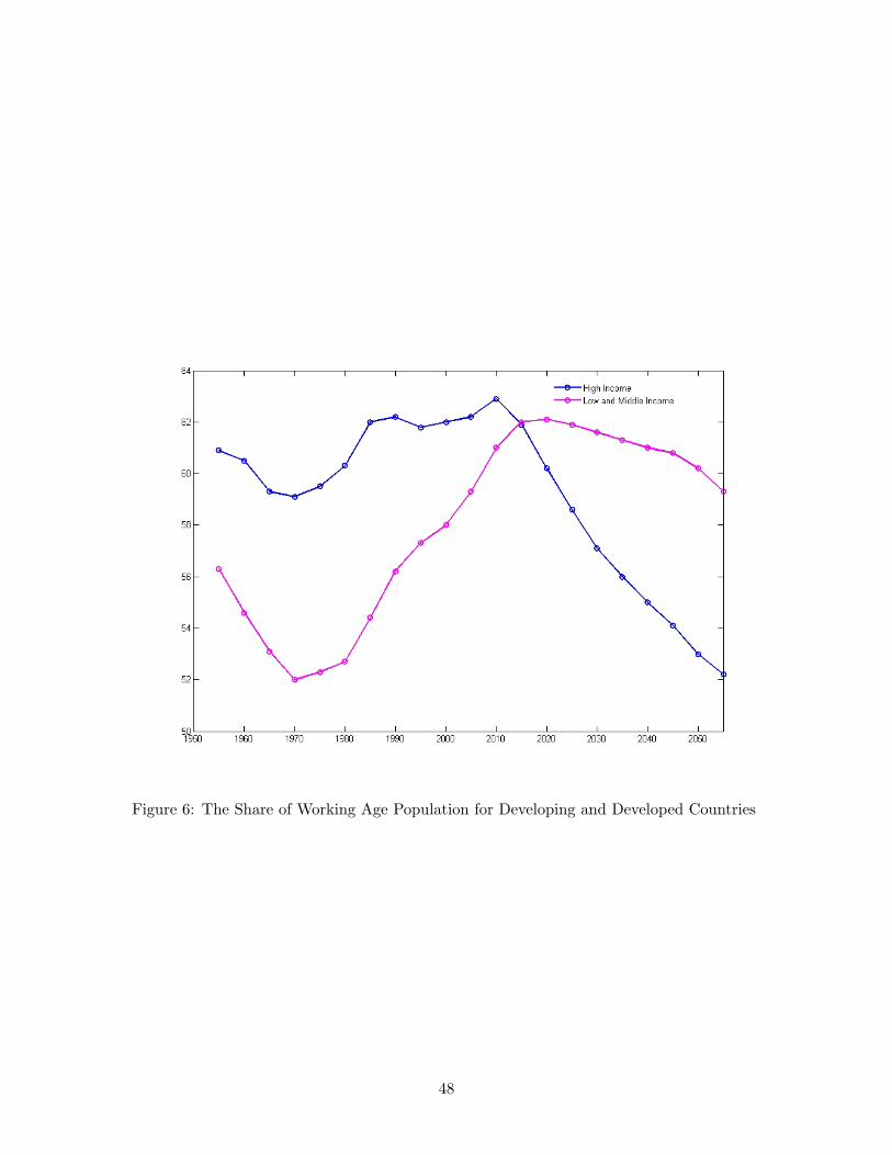
Figure 6: The Share of Working Age Population for Developing and Developed Countries

48

1989 1993 1998 2002 2006αc −0.47∗∗∗ −0.73∗∗∗ −0.60∗∗∗ −0.67∗∗∗ −0.75∗∗∗

(0.007) (0.008) (0.007) (0.006) (0.006)R2 0.32 0.32 0.29 0.25 0.27

Table 4: This table shows the estimated coefficient αc for developing countries as a whole over time. Standarderrors are in parentheses; ∗ ∗ ∗ denotes significance at the 1-percent level.

Pooled Pooled Pooled(2) Between Within F-E(1) (2) (3) (4) (5) (6)

αc −0.193∗∗∗ −0.19∗∗∗ −0.181∗∗ −0.30∗∗ −0.12∗∗∗ −0.23∗∗∗

(0.07) (0.074) (0.01) (0.127) (0.04) (0.07)Openness 1.98∗∗∗ 2.47∗∗∗ 1.54 −0.42 1.25

( 0.69) (0.124) (1.03) (0.28) (1.09)Annual GDP growth −0.03 0.29∗∗∗ 2.8 −0.1∗∗∗ -0.15

(0.074) (0.02) (12.7) (0.01) (0.07)Population growth -0.67∗∗ −0.65∗∗∗ -1.3 −0.22 −0.08

(0.27) (0.02) (13.5) ( 0.35) (0.38)Country Fixed Effect No No No - Yes YesYear Fixed Effect No No No - No Yes

R2 0.01 0.05 0.71 0.07 0.55 0.20Number of Observations 450 450 450 86 450 450

Table 5: This table reports the results of estimating CAct = α+β1 ·αct+γ′Zt+uct. Column (3) uses an alternativedefinition of the independent variable: the average CA/GDP over a period. The between regression reports the resultsusing country-averages of all variables, and including a constant. The within regression reports results using countryfixed effects, and (6) reports results using country and year fixed effects. Constants, country, and year effects arenot reported. The sample consists of the years t, 1989, 1993, 1998, 2002, 2006, for all countries. Additional controlsinclude GDP, and GDP per capita.

Pooled Pooled Within F-E(1) (2) (3) (4)

Share −0.03∗∗∗ −0.03∗∗∗ −0.25∗∗∗ −0.27∗∗∗

(0.005) (0.02) (0.01) (0.02)Annual GDP growth −0.05∗∗∗ 0.04∗∗∗ 0.03∗∗∗

(.0045) (0.005) (0.005)Initial Openness 0.62∗∗∗ 1.61∗∗∗ 1.85∗∗∗

(0.07) (0.17) (0.18)Initial Capital Stock 0 0 0Country Fixed Effect No No Yes YesYear Fixed Effect No No No Yes

R2 0.02 0.04 0.62 0.64Number of Observations 350 350 350 350

Table 6: This table reports the results of estimating αct = βc +Sharect +γ′Zct + εct. The within regression reportsresults using country fixed effects, and column (4) reports results using country and year fixed effects. Constants,country, and year effects are not reported. The sample consists of the years t, 1989, 1993, 1998, 2002, 2006, for allcountries. Additional controls include GDP per Capital, and population growth.

49

0 1 2 3 4 5 6 7 8 90.4

0.6

0.8

1

1.2

1.4

1.6

1.8

Anticipated Labor Force Boom Shock

Generations

Hom

e In

vest

men

t

shockTwo-sector Case

One-sector Case

Figure 7: An anticipated doubling of labor force in Foreign, in both the one and two-sector case.

50