Inductive Synthesis of Functional Programs: An …jmlr.csail.mit.edu/papers/volume7/kitzelmann06a/kit...An EBG Approach to Inductive Synthesis of Functional Programs Unfolding of an

Journal of Machine Learning Research 7 (2006) 429–454 Submitted 7/05; Revised 1/06; Published 2/06

Inductive Synthesis of Functional Programs:An Explanation Based Generalization Approach

Emanuel Kitzelmann [email protected]

Ute Schmid [email protected]

Department of Information Systems and Applied Computer ScienceOtto-Friedrich-UniversityBamberg, Germany

Editors: Roland Olsson and Leslie Pack Kaelbling

Abstract

We describe an approach to the inductive synthesis of recursive equations from input/output-examples which is based on the classical two-step approach to induction of functional Lispprograms of Summers (1977). In a first step, I/O-examples are rewritten to traces whichexplain the outputs given the respective inputs based on a datatype theory. These tracescan be integrated into one conditional expression which represents a non-recursive pro-gram. In a second step, this initial program term is generalized into recursive equationsby searching for syntactical regularities in the term. Our approach extends the classicalwork in several aspects. The most important extensions are that we are able to induce aset of recursive equations in one synthesizing step, the equations may contain more thanone recursive call, and additionally needed parameters are automatically introduced.Keywords: inductive program synthesis, inductive functional programming, explanationbased generalization, recursive program schemes

1. Introduction

Automatic induction of recursive programs from input/output-examples (I/O-examples) isan active area of research since the sixties and of interest for AI research as well as for soft-ware engineering (Lowry and McCarthy, 1991; Flener and Partridge, 2001). In the seventiesand eighties, there were several approaches to the synthesis of Lisp programs from examplesor traces (see Biermann et al. 1984 for an overview). The most influential approach wasdeveloped by Summers (1977), who put inductive synthesis on a firm theoretical foundation.

Summers’ early approach is an explanation based generalization (EBG) approach, thusit widely relies on algorithmic processes and only partially on search: In a first step, traces—steps of computations executed from a program to yield an output from a particular input—and predicates for distinguishing the inputs are calculated for each I/O-pair. Constructionof traces, which are terms in the classical functional approaches, relies on knowledge of theinductive datatype of the inputs and outputs. That is, traces explain the outputs basedon a theory of the used datatype given the respective inputs. The classical approaches forsynthesizing Lisp-programs used the general Lisp datatype S-expression. By integratingtraces and predicates into a conditional expression a non-recursive program explaining allI/O-examples is constructed as a result of the first synthesis step. In a second step, regular-

c©2006 Emanuel Kitzelmann and Ute Schmid.

Kitzelmann and Schmid

ities are searched for between the traces and predicates respectively. Found regularities arethen inductively generalized and expressed in the form of the resulting recursive program.

The programs synthesized by Summers’ system contain exactly one recursive function,possibly along with one constant term calling the recursive function. Furthermore, allsynthesizable functions make use of a small fixed set of Lisp-primitives, particularly ofexactly one predicate function, atom, which tests whether its argument is an atom, e.g.,the empty list. The latter implies two things: First, that Summers’ system is restricted toinduce programs for structural problems on S-expressions. That means, that execution ofinduced programs depends only on the structure of the input S-expression, but never onthe semantics of the atoms contained in it. For example, reversing a list is a structuralproblem, yet not sorting a list. The second implication is, that calculation of the traces isa deterministic and algorithmic process, i.e., does not rely on search and heuristics.

Due to only limited progress regarding the class of programs which could be inferred byfunctional synthesis, interest decreased in the mid-eighties. There was a renewed interest ofinductive program synthesis in the field of inductive logic programming (ILP) (Flener andYilmaz, 1999; Muggleton and De Raedt, 1994), in genetic programming and other forms ofevolutionary computation (Olsson, 1995) which rely heavily on search.

We here present an EBG approach which is based on the methodologies proposed bySummers (1977). We regard the functional two-step approach as worthwhile for the follow-ing reasons: First, algebraic datatypes provide guidance in expressing the outputs in termsof the inputs as the first synthesis step. Second, it enables a seperate and thereby special-ized handling of a knowledge dependent part and a purely syntactic driven part of programsynthesis. Third, using both algebraic datatypes and seperating a knowledge-dependentfrom a syntactic driven part enables a more accurate use of search than in ILP or evolu-tionary programming. Fourth, the two-step approach using algebraic datatypes provides asystematic way to introduce auxiliary recursive equations if necessary.

Our approach extends Summers in several important aspects, such that we overcomefundamental restrictions of the classical approaches to induction of Lisp programs: First, weare able to induce a set of recursive equations in one synthesizing step, second, the equationsmay contain more than one recursive call, and third, additionally needed parameters areautomatically introduced. Furthermore, our generalization step is domain-independent, inparticular independent from a certain programming language. It takes as input a first-orderterm over an arbitrary signature and generalizes it to a recursive program scheme, that is, aset of recursive equations over that signature. Hence it can be used as a learning componentin all domains which can represent their objects as recursive program schemes and provide asystem for solving the first synthesis step. For example, we use the generalization algorithmfor learning recursive control rules for AI planning problems (cp. Schmid and Wysotzki2000; Wysotzki and Schmid 2001).

2. Overview Over the Approach

The three central objects dealt with by our system are (1) sets of I/O-examples specifyingthe algorithm to be induced, (2) initial (program) terms explaining the I/O-examples, and(3) recursive program schemes (RPSs) representing the induced algorithms. Their func-tional role in our two-step synthesis approach is shown in Figure 1.

430

An EBG Approach to Inductive Synthesis of Functional Programs

I/O-examples

1. Step: Explanation, based

on knowledge of datatypes−−−−−−−−−−−−−−−−−−−−−→ Initial Term

2. Step: Generalization,

purely syntactic driven−−−−−−−−−−−−−−−−−−→ RPS

Figure 1: Two synthesis steps

2.1 First Synthesis Step: From I/O-examples to an Initial Term

An example for I/O-examples is given in Table 1. The examples specify the lasts functionwhich takes a list of lists as input and yields a list of the last elements of the lists asoutput. In the first synthesis step, an initial term is constructed from these examples. An

[] 7→ [],[[a]] 7→ [a],

[[a, b]] 7→ [b],[[a, b, c], [d]] 7→ [c, d],

[[a, b, c, d], [e, f ]] 7→ [d, f ],[[a], [b], [c]] 7→ [a, b, c]

Table 1: I/O-examples for lasts

initial term is a term respecting an arbitrary first-order signature extended by the specialconstant symbol Ω, meaning the undefined value and directing generalization in the secondsynthesis step. Suitably interpreted, an initial term evaluates to the specified output whenits variable is instantiated with a particular input of the example set and to undefined forall other inputs.

Table 2 gives an example of an initial term. It shows the result of applying the firstsynthesis step to the I/O-examples for the lasts function as shown in Table 1. if meansthe 3ary non-strict function which returns the value of its second parameter if its firstparameter evaluates to true and otherwise returns the value of its third parameter; emptyis a predicate which tests, whether its argument is the empty list; head and tail yield thefirst element and the rest of a list respectively; cons constructs a list from one element anda list; and [] denotes the empty list.

Calculation of initial terms relies on knowledge of the datatypes of the example inputsand outputs. For our exemplary lasts program inputs and outputs are lists. Lists areuniquely constructed by means of the empty list [] and the constructor cons. Furthermore,they are uniquely decomposed by the functions head and tail . That allows to calculatea unique term which expresses an example output in terms of the input. For example,consider the fourth I/O-example from Table 1: If x denotes the input [[a, b, c], [d]], then theterm cons(head(tail(tail(head(x)))), head(tail(x))) expresses the specified output [c, d] interms of the input. Such traces are constructed for each I/O-pair. The overall concept forintegrating the resulting traces into one initial term is to go through all traces in parallelposition by position. If the same function symbol is contained at the current position in alltraces, then it is introduced to the initial term at this position. If at least two traces differat the current position, then an if -expression is introduced. Therefore a predicate functionis calculated to discriminate the inputs according to the different traces. Constructionof the initial term proceeds from the discriminated inputs and traces for the second and

431


if(empty(x), [],cons(head(if(empty(tail(head(x))), head(x),if(empty(tail(tail(head(x)))), tail(head(x)),if(empty(tail(tail(tail(head(x))))), tail(tail(head(x))),Ω)))),

if(empty(tail(x)), [],cons(head(if(empty(tail(head(tail(x)))), head(tail(x)),Ω)),

if(empty(tail(tail(x))), [],Ω)))))))

Table 2: Initial term for lasts

third branch of the if -tree respectively. We describe the calculation of initial terms fromI/O-examples, i.e., the first synthesis step, in Section 4.

2.2 Second Synthesis Step: From Initial Terms to Recursive Equations

In the second synthesis step, initial ground terms are generalized to a recursive programscheme. Initial terms are considered as (incomplete) unfoldings of an RPS which is to beinduced by generalization. An RPS is a set of recursive equations whose left-hand-sidesconsist of the names of the equations followed by their parameter lists and whose right-hand-sides consist of terms over the signature from the initial terms, the set of the equationnames, and the parameters of the equations. One equation is distinguished to be the mainone. An example is given in Table 3. This RPS, suitably interpreted, computes the lastsfunction as described above and specified by the examples in Table 1. It results from

lasts(x) = if(empty(x), [], cons(head(last(head(x))), lasts(tail(x))))

last(x) = if(empty(tail(x)), x, last(tail(x)))

Table 3: Recursive Program Scheme for lasts

applying the second synthesis step to the initial term shown in Table 2. Note that it is ageneralization from the initial term in that it not merely computes the lasts function for theexample inputs but for input-lists of arbitrary length containing lists of arbitrary length.

The second synthesis step does not depend on domain knowledge. The meaning of thefunction symbols is irrelevant, because the generalization is completely driven by detectingsyntactical regularities in the initial terms. To understand the link between initial termsand RPSs induced from them, we consider the process of incrementally unfolding an RPS.

432


Unfolding of an RPS is a (non-deterministic and possibly infinite) rewriting process whichstarts with the instantiated head of the main equation of an RPS and which repeatedlyrewrites a term by substituting any instantiated head of an equation in the term witheither the equally instantiated body or with the special symbol Ω. Unfolding stops, whenall heads of recursive equations in the term are rewritten to Ω, i.e., the term contains norewritable head any more. Consider the last equation from the RPS shown in Table 3 andthe initial instantiation x 7→ [a, b, c]. We start with the instantiated head last([a, b, c])and rewrite it to the term:

if(empty(tail([a, b, c])), [a, b, c], last(tail([a, b, c])))

This term contains the head of the last equation instantiated with x 7→ tail([a, b, c]).When we rewrite this head again with the equally instantiated body we obtain:

if(empty(tail([a, b, c])), [a, b, c],if(empty(tail(tail([a, b, c]))), tail([a, b, c]),

last(tail(tail([a, b, c]))))

This term now contains the head of the equation instantiated with x 7→ tail(tail([a, b, c])).We rewrite it once again with the instantiated body and then replace the head in theresulting term with Ω and obtain:

if(empty(tail([a, b, c])), [a, b, c],if(empty(tail(tail([a, b, c]))), tail([a, b, c]),

if(empty(tail(tail(tail([a, b, c])))), tail(tail([a, b, c])),Ω)))

The resulting finite term of a finite unfolding process is also called unfolding. Unfoldingsof RPSs contain regularities if the heads of the recursive equations are more than oncerewritten with its bodies before they are rewritten with Ωs. The second synthesis step isbased on detecting such regularities in the initial terms.

We describe the generalization of initial terms to RPSs in Section 3. The reason whywe first describe the second synthesis step and only afterwards the first synthesis step is,that the latter is governed by the goal of constructing a term which can be generalized inthe second step. Therefore, for understanding the first step, it is necessary to know theconnection between initial terms and RPSs as established in the second step.

2.3 Characteristics and Limitations of the Approach

The overall objective of our approach is automatical induction of recursive functional pro-grams from I/O-examples which are correct with respect to the functional behaviour desiredby the user. Since the approach is based on finding differences between traces, i.e., analyzingone example in relation to the following example, the examples have to be the first k exam-ples according to an ordering of the underlying data-type with the first example beeing theleast complex instance for which the target recursive program is defined. This is in contrastto learning from a randomly chosen set of training data (according to some distribution)which is the common setting in most learning approaches, e.g., in all PAC-learning (Valiant,1984) algorithms. Another implication of this generalization methodology is that very few

433


examples are sufficient. This is again in contrast to most learning settings, especially incontrast to the identification-in-the-limit setting (Gold, 1967). A third implication is thatthe examples have to be correct, i.e., the desired function has to be consistent with theexamples. This is not a limitation in our view since we assume that the examples are givenby some (end-user) programmer who knows the functional behaviour of the target programand thus can provide a few correct examples. A fourth implication of the example-drivenapproach is, that termination is assured for the induced programs. This is an importantcharacteristic since in general, termination is not decidable. Our algorithms output a setof recursive equations which are consistent with the I/O-examples, i.e., which compute anyspecified example-output from the respective example-input.

There are restrictions regarding the programs which can be synthesized. The first step(see Section 2.1 for an overview and Section 4 for details) is restricted to structural problems,i.e., functions on lists may only depend on the list structure but not on the meaning of theitems in the lists. The induced recursive equations stand in some call-relation. Due tothe second synthesis step (see Section 2.2 for an overview and Section 3 for details), thisrelation is restricted to be flat, that is, recursive calls cannot be nested. Furthermore, therelation is non-mutual, i.e., if one equation calls a second one, then the second one cannotcall the first one. Since the induction process relies on two successive synthesis steps, theoverall restrictions are the sum of the restrictions of the first step and the restrictions of thesecond step. On the other hand, the two-step approach provides some modularity. Since thelimitation to structural problems is a restriction of only the first step, it would be sufficientto only extend or substitute the first step to extend our approach to be capable of dealingwith non-structural problems, e.g., sorting problems.

For experimental results, a discussion of the approach, and a comparison to other in-ductive programming systems see Sections 5 and 6.

3. Generalizing an Initial Term to an RPS

Since our generalization algorithm exploits the relation between an RPS and its unfoldings,in the following we will first introduce the basic terminology for terms, substitutions, andterm rewriting as for example presented in Dershowitz and Jouanaud (1990). Then we willpresent definitions for RPSs and the relation between RPSs and their unfoldings. The setof all possible RPSs constitutes the hypothesis language for our induction algorithm. Somerestrictions on this general hypothesis language are introduced and finally, the componentsof the generalization algorithm are described.

3.1 Preliminaries

We denote the set of natural numbers starting with 0 by N and the natural numbers greaterthan 0 by N+. A signature Σ is a set of (function) symbols with α : Σ→ N giving the arityof a symbol. We write TΣ for the set of ground terms, i.e., terms without variables, over Σand TΣ(X) for the set of terms over Σ and a set of variables X. We write TΣ,Ω for the set ofground terms—called partial ground terms—constructed over Σ∪Ω, where Ω is a specialconstant symbol denoting the undefined value. Furthermore, we write TΣ,Ω(X) for the setof partial terms constructed over Σ∪Ω and variables X. With T∞Σ,Ω(X) we denote the setof inifinite partial terms over Σ and variables X. Over the sets TΣ,Ω, TΣ,Ω(X) and T∞Σ,Ω(X)

434


a complete partial order (CPO) ≤ is defined by: a) Ω ≤ t for all t ∈ TΣ,Ω, TΣ,Ω(X), T∞Σ,Ω(X)and b) f(t1, . . . , tn) ≤ f(t′1, . . . , t

′n) iff ti ≤ t′i for all i ∈ [1;n].

Terms can uniquely be expressed as labeled trees: If a term is a constant symbol ora variable, then the corresponding tree consists of only one node labeled by the constantsymbol or variable. If a term has the form f(t1, . . . , tn), then the root node of the corre-sponding tree is labeled with f and contains from left to right the subtrees correspondingto t1, . . . , tn. We use the terms tree and term as synonyms. A position of a term/tree isa sequence of positive natural numbers, i.e., an element from N ∗

+ . The set of positions ofa term t, denoted pos(t), contains the empty sequence ε and the position iu, if the termhas the form t = f(t1, . . . , tn) and u is a position from pos(ti), i ∈ [1;n]. Each positionof a term uniquely denotes one subterm. We write t|u for denoting that subterm which isdetermined as follows: (a) t|ε = t, (b) if t = f(t1, . . . , tn) and u is a position in ti, thent|iu = ti|u, i ∈ [1;n]. E.g., for the term f(x, y, g(h(a, p(s, t), b), z)) the position 312 denotesthe subterm p(s, t) because it is the second subterm of the first subterm of the third subtermof the original term. We say that position u is smaller than position u′, u ≤ u′, if u is aprefix of u′. If u is a position of term t and u′ ≤ u, then u′ is a position of t. For a term tand a position u, node(t, u) denotes the fixed symbol f ∈ Σ, if t|u = f(t1, . . . , tn) or t|u = frespectively. The set of all positions at which a fixed symbol f appears in a term is denotedby pos(t, f). The replacement of a subterm t|u by a term s in a term t at position u iswritten as t[u← s]. Let U denote a set of positions in a term t. Then t[U ← s] denotes thereplacement of all subterms t|u with u ∈ U by s in t.

A substitution σ is a mapping from variables to terms. Substitutions are naturallycontinued to mappings from terms to terms by σ(f(t1, . . . , tn)) = f(σ(t1), . . . , σ(tn)). Sub-stitutions are written in postfix notation, i.e., we write tσ instead of σ(t). Substitutionsβ : X → TΣ from variables to ground terms are called (variable) instantiations. A term p iscalled pattern of a term t, iff t = pσ for a substitution σ. A pattern p of a term t is calledtrivial, iff p is a variable and non-trivial otherwise. We write t ≤s p iff p is a pattern of tand t <s p iff additionally holds, that p and t can not be unified by variable renaming only.

A term rewriting system (TRS) over Σ and X is a set of pairs of terms R ⊆ TΣ(X) ×TΣ(X). The elements (l, r) of R are called rewrite rules and are written l → r. A term t′

can be derived in one rewrite step from a term t using R (t→R t′), if there exists a positionu in t, a rule l → r ∈ R, and a substitution σ : X → TΣ(X), such that (a) t|u = lσ and(b) t′ = t[u ← rσ]. R implies a rewrite relation →R⊆ TΣ(X) × TΣ(X) with (t, t′) ∈→R ift→R t′.

3.2 Recursive Program Schemes

Definition 1 (Recursive Program Scheme) Given a signature Σ, a set of functionvariables Φ = G1, . . . , Gn for a natural number n > 0 with Σ∩Φ = ∅ and arity α(Gi) > 0for all i ∈ [1;n], a natural number m ∈ [1;n], and a set of equations

G =

G1(x1, . . . , xα(G1)) = t1,

...Gn(x1, . . . , xα(Gn)) = tn

435


where the ti are terms with respect to the signature Σ ∪ Φ and the variables x1, . . . , xα(Gi),S = (G,m) is an RPS. Gm(x1, . . . , xα(Gm)) = tm is called the main equation of S.

The function variables in Φ are called names of the equations, the left-hand-sides are calledheads, the right-hand-sides bodies of the equations. For the lasts RPS shown in Table 3holds: Σ = if , empty , cons, head , tail , [], Φ = G1, G2 with G1 = lasts and G2 = last ,and m = 1. G is the set of the two equations.

We can identify a TRS with an RPS S = (G,m):

Definition 2 (TRS implied by an RPS) Let S = (G,m) be an RPS over Σ, Φ andX, and Ω the bottom symbol in TΣ,Ω(X). The equations in G constitute rules RS =Gi(x1, . . . , xα(Gi)) → ti | i ∈ [1;n] of a term rewriting system. The system addition-ally contains rules RΩ = Gi(x1, . . . , xα(Gi))→ Ω | i ∈ [1;n], Gi is recursive.

The standard interpretation of an RPS, called free interpretation, is defined as thesupremum in T∞Σ,Ω(X) of the set of all terms in TΣ,Ω(X) which can be derived by theimplied TRS from the head of the main equation. Two RPSs are called equivalent, iffthey have the same free interpretation, i.e., if they compute the same function for everyinterpretation of the symbols in Σ. Terms in TΣ,Ω which can be derived by the instantiatedhead of the main equation regarding some instantiation β : X → TΣ are called unfoldingsof an RPS relative to β. Note, that terms derived from RPSs are partial and do not containfunction variables, i.e., all heads of the equations are eventually rewritten by Ωs.

The goal of the generalization step is to find an RPS which explains a set of initialterms, i.e., to find an RPS such that the initial terms are unfoldings of that RPS. Wedenote initial terms by t and a set of initial terms by I. We liberalize I such that it mayinclude incomplete unfoldings. Incomplete unfoldings are unfoldings, where some subtreescontaining Ωs are replaced by Ωs.

We need to define four further concepts, namely recursion positions which are positionsin the equation bodies where recursive calls appear, substitution terms which are the argu-ment terms in recursive calls, unfolding positions which are positions in unfoldings at whichthe heads of the equations are rewritten with their bodies, and finally parameter instanti-ations in unfoldings which are subterms of unfoldings resulting from the initial parameterinstantiation and the substitution terms:

Definition 3 (Recursion Positions and Substitution Terms) Let G(x1, . . . , xα(G)) =t with parameters X = x1, . . . , xα(G) be a recursive equation. The set of recursion posi-tions of G is given by R = pos(t, G). Each recursive call of G at position r ∈ R in t impliessubstitutions σr : X → TΣ(X) : xj 7→ t|rj for all j ∈ [1;α(G)] for the parameters in X. Wecall the terms t|rj substitution terms of G.

For equation lasts of the lasts RPS (Table 3) holds R = 32 and xσ32 = tail(x). Forequation last holds R = 3 and xσ3 = tail(x).

Now consider an unfolding process of a recursive equation and the positions at whichrewrite steps are applied in the intermediate terms. The first rewriting is applied at root-position ε, since we start with the instantiated head of the equation which is completelyrewritten with the instantiated body. In the instantiated body, rewrites occur at recursion

436


positions R. Assume that on recursion position r ∈ R the instance of the head is rewrittenwith an instance of the body. Then, relative to the resulting subtree at position r, rewritesoccur again at recursion positions, e.g., at position r′ ∈ R. Relative to the entire term theselatter rewrites occur therefore at compositions of position r and recursion positions, e.g.,at position rr′ and so on. We call the infinite set of positions at which rewrites can occurin the intermediate terms within an unfolding of a recursive equation unfolding positions.They are determined by the recursion positions as follows:

Definition 4 (Unfolding Positions) Let R be the recursion positions of a recursive equa-tion G. The set of unfolding positions U of G is defined as the smallest set of positionswhich contain the position ε and, if u ∈ U and r ∈ R, the position ur.

The unfolding positions of equation lasts of the lasts RPS are 32, 3232, 323232, . . ..Now we look at the variable instantiations occuring during unfolding a recursive equa-

tion. Recall the unfolding process of the last equation (see Table 3) described at the end ofSection 2.2. The initial instantiation was βε = β = x 7→ [a, b, c], thus in the body of theequation (replaced for the instantiated head as result of the first rewrite step), its variableis instantiated with this initial instantiation. Due to the substitution term tail(x), the vari-able of the head in this body is instantiated with β3 = σ3 βε = x 7→ tail([a, b, c]), i.e., thevariable in the body replaced for this instantiated head is instantiated with σ3 βε. A furtherrewriting step implies the instantiation β33 = σ3 σ3 βε = σ3 β3 = x 7→ tail(tail([a, b, c]))and so on. We index the instantiations occuring during unfolding with the unfolding posi-tions at which the particular instantiated heads were placed. They are determined by thesubstitutions implied by recursive calls and an initial instantiation as follows:

Definition 5 (Instantiations in Unfoldings) Let G(x1, . . . , xα(G)) = t be a recursiveequation with parameters X = x1, . . . , xα(G), R and U the recursion positions and unfold-ing positions of G resp., σr the substitutions implied by the recursive call of G at positionr ∈ R, and β : X → TΣ an initial instantiation. Then a family of instantiations indexedover U is defined as βε = β and βur = σr βu for u ∈ U, r ∈ R.

3.3 Restrictions and the Generalization Problem

An RPS which can be induced from initial terms is restricted in the following way: First,it contains no mutual recursive equations, second, there are no calls of recursive equationswithin calls of recursive equations (no nested recursive calls). The first restriction is not asemantical restriction, since each mutual recursive program can be transformed to an equiv-alent (regarding a particular algebra) non-mutual recursive program. Yet it is a syntacticalrestriction, since unfoldings of mutual RPSs can not be generalized using our approach. Arestriction similar to the second one was stated by Rao (2004). He names TRSs complyingwith such a restriction flat TRSs.

Inferred RPSs conform to the following syntactical characteristics: First, all equations,potentially except of the main equation, are recursive. The main equation may be recursiveas well, but, it is the only equation not required to be recursive. Second, inferred RPSs areminimal, in that (i) each equation is directly or indirectly (by means of other equations)called from the main equation, and (ii) no parameter of any equation can be omitted

437


if

empty

x

x

tail

tail

head

tail

tail

tail

head

Omega

if

if

cons

if

if

cons

if

if

[]

x

empty

x

empty

x

[]empty

[]empty

empty

x

empty

x

x

x

x

x

head

tail

head

head

tail

tail

head

tail

head

tail

tail

head

tail

head

head

tail

tail

tail

Omega

Omega

Figure 2: Initial Tree for lasts

without changing the free interpretation. RPSs complying with the stated restrictions andcharacteristics are called minimal, non-mutual, flat recursive program schemes.

There might be several RPSs which explain an initial term t, but have different freeinterpretations. For example, Ω is an unfolding of every RPS with a recursive main equation.Therefore, an important question is which RPS will be induced. Summers (1977) requiredthat recurrence relations hold at least over three succeeding traces and predicates to justifya generalization. A similar requirement would be that induced RPSs explain the initialterms recurrently, meaning that I contains at least one term t which can be derived froman unfolding process, in which each recursive equation had to be rewritten at least threetimes with its body. We use a slightly different requirement: One characteristic of minimalRPSs is, that if at least one substitution term is replaced by another, then the resultingRPS has a different free interpretation. We call this characteristic substitution uniqueness.Thus, it is sensible to require that induced RPSs are substitution unique regarding theinitial terms, i.e., that if some substitution term is changed, then the resulting RPS nolonger explains the initial terms. It holds, that a minimal RPS explains a set of initial treesrecurrently, if it explains it substitution uniquely.

Thus the problem of generalizing a set of initial terms I to an RPS is to find an RPSwhich explains I and which is substitution unique regarding I.

3.4 Solving the Generalization Problem

We will not state the generalization algorithm in detail in this section but we will describethe underlying concepts and the algorithm in a more informal manner. For this section andits subsections we use the term body of an equation for terms which are strictly speakingincomplete bodies: They contain only the name of the equation instead of complete recursivecalls including substitution terms at recursion positions. For example, we refer to the termif (empty(x), [], cons(head(last(head(x))), lasts)) as the body for equation lasts of the lasts

438


RPS (see Table 3). The reason is, that we infer the complete body in two steps: First theterm which we name body in this context, second the substitution terms for the recursivecalls.

Generalization of a set of initial terms to an RPS is done in three successive steps,namely segmentation of the terms, construction of equation bodies and calculation of sub-stitution terms. These three generalization steps are organized in a divide-and-conqueralgorithm, where backtracking can occur to the divide-phase. Segmentation constitutes thedivide-phase which proceeds top-down through the initial terms. Within this phase recur-sion positions (see Definition 3) and positions indicating further recursive equations aresearched for each induced equation. The latter set of positions is called subscheme positions(see Definition 6 below). Found recursion positions imply unfolding positions (see Defini-tion 4). As a result of the divide-phase the initial terms are divided into several parts bythe subscheme positions, such that—roughly speaking—each particular part is assumed tobe an unfolding of one recursive equation. Furthermore, the particular parts are segmentedby the unfolding positions, such that—roughly speaking—each segment is assumed to bethe result of one unfolding step of the respective recursive equation.

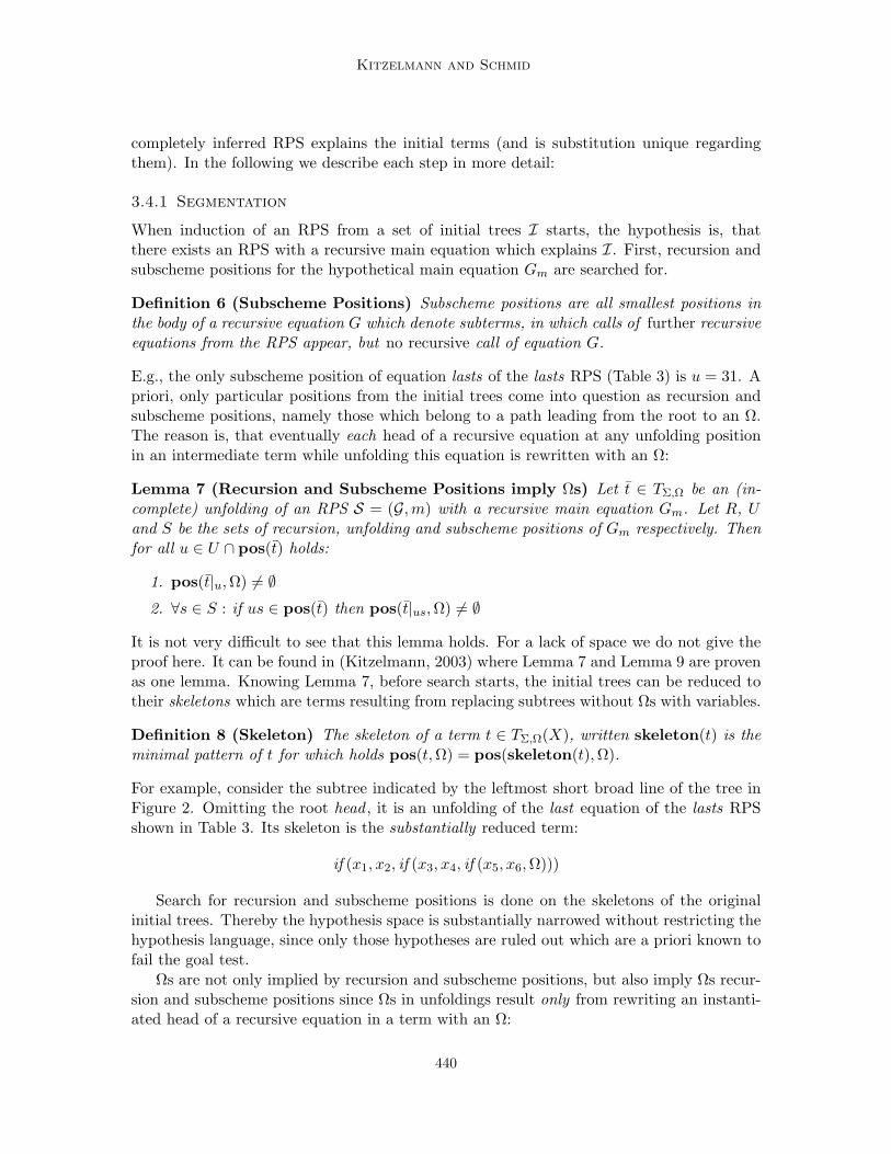
Consider the initial tree in Figure 2, it represents the initial term for lasts, shown inTable 2. The curved lines on the path to the rightmost Ω divide the tree into three segmentswhich correspond to unfolding steps of the main equation, i.e., equation lasts. Note, thatthe rightmost segment is incomplete. The short broad lines denote two subtrees whichare—except of their root head—unfoldings of the last equation. The curved lines withinthese subtrees divide each subtree into segments, such that each segment corresponds toone unfolding step of the last equation.

When the initial trees are segmented, calculation of equation bodies and of substitutionterms follows within the conquer-phase. These two steps proceed bottom-up through thedivided initial trees and reduce the trees during this process. The effect is, that bodies andsubstitution terms for each equation are calculated from trees which are unfoldings of onlythe currently induced equation and hence, each segment in these trees is an instantiationof the body of the currently induced equation. For example, for the lasts tree shown inFigure 2, a body and substitution terms are first calculated from the two subtrees, i.e.,for the last equation. Since there are no further recursive equations called by the lastequation—i.e., the segments of the two subtrees contain themselves no subtrees which areunfoldings of further equations—each segment is an instantiation of the body of the lastequation. When this equation is completely inferred, the two subtrees are replaced bysuitable instantiations of the head of the inferred last equation. The resulting reduced treeis an unfolding of merely one recursive equation, the lasts equation. The three segmentsin this reduced tree—indicated by the curved lines on the path to the rightmost Ω—areinstantiations of the body of the searched for lasts equation. From this reduced tree, bodyand substitution terms for the lasts equation are induced and the RPS is completely induced.

Segmentations are searched for, whereas calculation of bodies and substitution termsare algorithmic. Construction of bodies always succeeds, whereas calculation of substitutionterms—such that the inferred RPS explains the initial terms—may fail. Thus, an inferredRPS can be seen as the result of a search through a hypothesis space where the hypothesesare segmentations (divide-phase), and a constructive goal test, including construction ofbodies and calculation of substitution terms (conquer-phase), which tests, whether the

439


completely inferred RPS explains the initial terms (and is substitution unique regardingthem). In the following we describe each step in more detail:

3.4.1 Segmentation

When induction of an RPS from a set of initial trees I starts, the hypothesis is, thatthere exists an RPS with a recursive main equation which explains I. First, recursion andsubscheme positions for the hypothetical main equation Gm are searched for.

Definition 6 (Subscheme Positions) Subscheme positions are all smallest positions inthe body of a recursive equation G which denote subterms, in which calls of further recursiveequations from the RPS appear, but no recursive call of equation G.

E.g., the only subscheme position of equation lasts of the lasts RPS (Table 3) is u = 31. Apriori, only particular positions from the initial trees come into question as recursion andsubscheme positions, namely those which belong to a path leading from the root to an Ω.The reason is, that eventually each head of a recursive equation at any unfolding positionin an intermediate term while unfolding this equation is rewritten with an Ω:

Lemma 7 (Recursion and Subscheme Positions imply Ωs) Let t ∈ TΣ,Ω be an (in-complete) unfolding of an RPS S = (G,m) with a recursive main equation Gm. Let R, Uand S be the sets of recursion, unfolding and subscheme positions of Gm respectively. Thenfor all u ∈ U ∩ pos(t) holds:

1. pos(t|u,Ω) 6= ∅2. ∀s ∈ S : if us ∈ pos(t) then pos(t|us,Ω) 6= ∅

It is not very difficult to see that this lemma holds. For a lack of space we do not give theproof here. It can be found in (Kitzelmann, 2003) where Lemma 7 and Lemma 9 are provenas one lemma. Knowing Lemma 7, before search starts, the initial trees can be reduced totheir skeletons which are terms resulting from replacing subtrees without Ωs with variables.

Definition 8 (Skeleton) The skeleton of a term t ∈ TΣ,Ω(X), written skeleton(t) is theminimal pattern of t for which holds pos(t, Ω) = pos(skeleton(t),Ω).

For example, consider the subtree indicated by the leftmost short broad line of the tree inFigure 2. Omitting the root head , it is an unfolding of the last equation of the lasts RPSshown in Table 3. Its skeleton is the substantially reduced term:

if (x1, x2, if (x3, x4, if (x5, x6,Ω)))

Search for recursion and subscheme positions is done on the skeletons of the originalinitial trees. Thereby the hypothesis space is substantially narrowed without restricting thehypothesis language, since only those hypotheses are ruled out which are a priori known tofail the goal test.

Ωs are not only implied by recursion and subscheme positions, but also imply Ωs recur-sion and subscheme positions since Ωs in unfoldings result only from rewriting an instanti-ated head of a recursive equation in a term with an Ω:

440


Lemma 9 (Ωs imply recursion and subscheme positions) Let t ∈ TΣ,Ω be an (in-complete) unfolding of an RPS S = (G,m) with a recursive main equation Gm. Let R, Uand S be the sets of recursion, unfolding and subscheme positions of Gm respectively. Thenfor all v ∈ pos(t, Ω) hold

• It exists an u ∈ U ∩ pos(t), r ∈ R with u ≤ v < ur or

• it exists an u ∈ U ∩ pos(t), s ∈ S with us ≤ v.

Proof: in (Kitzelmann, 2003).

From the definition of subscheme positions and the previous lemma follows, that subschemepositions are determined, if a set of recursion positions has been fixed. Lemma 7 restricts theset of positions which come into question as recursion and subscheme positions. Lemma 9together with characteristics from subscheme positions suggests to organize the search as asearch for recursion positions with a depending parallel calculation of subscheme positions.When hypothetical recursion, unfolding, and subscheme positions are determined they arechecked regarding the labels in the initial trees on pathes leading to Ωs. The nodes betweenone unfolding position and its successors in unfoldings result from the same body (withdifferent instantiations). Since variable instantiations only occur in subtrees at positionsnot belonging to pathes leading to Ωs, for each unfolding position the nodes between it andits successors are necessarily equal :

Lemma 10 (Valid Segmentation) Let t ∈ TΣ,Ω be an unfolding of an RPS S = (G,m)with a recursive main equation Gm. Then there exists a term tG ∈ TΣ,Ω(X) with pos(tG,Ω) =R∪S such that for all u ∈ U ∩pos(t) hold: tG ≤Ω t|u where ≤Ω is defined as (a) Ω ≤Ω t ifpos(t,Ω) 6= ∅, (b) x ≤Ω t if x ∈ X and pos(t, Ω) = ∅, and (c) f(t1, . . . , tn) ≤Ω f(t′1, . . . , t

′n)

if ti ≤Ω t′i for all i ∈ [1;n].Proof: in (Kitzelmann, 2003).

This lemma has to be slightly extended, if one allows for initial trees which are incompleteunfoldings. Lemma 10 states the requirements to assumed recursion and subscheme posi-tions which can be assured at segmentation time. They are necessary for an RPS whichexplains the initial terms, yet not sufficient to assure, that an RPS complying with themexists which explains the initial trees. That is, later a backtrack can occur to search forother sets of recursion and subscheme positions. If found recursion and subscheme positionsR and S comply with the stated requirements, we call the pair (R, S) a valid segmentation.

In our implemented system the search for recursion positions is organized as a greedysearch through the space of sets of positions in the skeletons of the initial trees. Whena valid segmentation has been found, compositions of unfolding and subscheme positionsdenote subtrees in the initial trees assumed to be unfoldings of further recursive equations.Segmentation proceeds recursively on each set of (sub)trees denoted by compositions ofunfolding positions and one subscheme position s ∈ S. We denote such a set of initial(sub)trees Is.

3.4.2 Construction of Equation Bodies

Construction of each equation body starts with a set of initial trees I for which at segmen-tation time a valid segmentation (R, S) has been found, and an already inferred RPS for

441


each subscheme position s ∈ S which explains the subtrees Is. These subtrees of the treesin I are replaced by the suitably instantiated heads or respectively bodies of the main equa-tions of the already inferred RPSs. For example, consider the initial tree for lasts shown inFigure 2. When calculation of a body for the main equation lasts starts from this tree, anRPS containing only the last equation which explains all three subtrees indicated by theshort broad lines has already been inferred. The initial tree is reduced by replacing thesethree subtrees by suitable instantiations of the head of the last equation. We denote the setof reduced initial trees also with I and its elements also with t. By reducing the initial treesbased on already inferred recursive equations, the problem of inducing a set of recursiveequations is reduced to the problem of inducing merely one recursive equation (where therecursion positions are already known from segmentation).

An equation body is induced from the segments of an initial tree which is assumed tobe an unfolding of one recursive equation.

Definition 11 (Segments) Let t be an initial tree, R a set of (hypothetical) recursionpositions and U the corresponding set of unfolding positions. The set of complete segmentsof t is defined as: t|u[R← G] | u ∈ U ∩ pos(t), R ⊂ t|u

For example, consider the subtree indicated by the leftmost short broad line of the initialtree in Figure 2 without its root head . It is an unfolding of the last equation as stated inTable 3. When the only recursion position 3 has been found it can be splitted into threesegments, indicated by the curved lines:

1. if(empty(tail(head(x))),head(x), G)

2. if(empty(tail(tail(head(x)))), tail(head(x)), G)

3. if(empty(tail(tail(tail(head(x))))), tail(tail(head(x))), G)

Expressed according to segments, the fact of a repetitive pattern between unfolding positions(see Lemma 10) becomes the fact, that the sequences of nodes between the root and eachG are equal for each segment. Each segment is an instantiation of the body of the currentlyinduced equation. In general, the body of an equation contains other nodes among thosebetween its root and the recursive calls. These further nodes are also equal in each segment.Differences in segments of unfoldings of a recursive equation can only result from differentinstantiations of the variables of the body. Thus, for inducing the body of an equationfrom segments, we assume each position in the segments which is equally labeled in allsegments as belonging to the body of the assumed equation, but each position which isvariably labeled in at least two segments as belonging to the instantiation of a variable.This assumption can be seen as an inductive bias since it might occur, that also positionswhich are equal over all segments belong to a variable instantiation. Nevertheless it holds,that if an RPS exists which explains a set of initial trees, then there also exists an RPSwhich explains the initial trees and is constructed based on the stated assumption. Basedon the stated assumption, the body of the equation to be induced is determined by thesegments and defined as follows:

Definition 12 (Valid Body) Given a set of reduced initial trees, the most specific maxi-mal pattern of all segments of all the trees is called valid body and denoted tG.

442


The maximal pattern of a set of terms can be calculated by first order anti-unification(Plotkin, 1969).

Calculating a valid body regarding the three segments enumerated above results inthe term if (empty(tail(x)), x,G). The different subterms of the segments are assumedto be instantiations of the parameters in the calculated valid body. Since each segmentcorresponds to one unique unfolding position, instantiations of parameters in unfoldings asdefined in Definition 5 are now given. For example, from the three segments enumeratedabove we obtain:

1. βε(x) = head(x)

2. β3(x) = tail(head(x))

3. β33(x) = tail(tail(head(x)))

3.4.3 Inducing Substitution Terms

Induction of substitution terms for a recursive equation starts on a set of reduced initialtrees which are assumed to be unfoldings of one recursive equation, an already inferred(incomplete) equation body which contains only a G at recursion positions, and variableinstantiations in unfoldings according to Definition 5. The goal is to complete each occurenceof G to a recursive call including substitution terms for the parameters of the recursiveequation.

The following lemma follows from Definition 5 and states characteristics of parameterinstantiations in unfoldings more detailed. It characterizes the instantiations in unfoldingsagainst the substitution terms of a recursive equation considering each single position inthem.

Lemma 13 (Instantiations in Unfoldings) Let G(x1, . . . , xα(G)) = t be a recursive equa-tion with parameters X = x1, . . . , xα(G), recursion positions R and unfolding positions U ,β : X → TΣ an instantiation, σr substitution terms for each r ∈ R and βu instantiations asdefined in Definition 5 for each u ∈ U . Then for all i, j ∈ [1;α(G)] and positions v hold:

1. If (xi σr)|v = xj then for all u ∈ U hold (xiβur)|v = xjβu.

2. If (xi σr)|v = f((xi σr)|v1, . . . , (xi σr)|vn), f ∈ Σ, α(f) = n then for all u ∈ U holdnode(xiβur, v) = f .

We can read the implications stated in the lemma in the inverted direction and thus weget almost immediately an algorithm to calculate the substitution terms of the searched forequation from the known instantiations in unfoldings.

One interesting case is the following: Suppose a recursive equation, in which at leastone of its parameters only occurs within a recursive call in its body, for example the equa-tion G(x, y, z) = if (zerop(x), y,+(x,G(prev(x), z, succ(y)))) in which this is the case forparameter z.1 For such a variable no instantiations in unfoldings are given when inductionof substitution terms starts. Also such variables are not contained in the (incomplete) valid

1. A practical example is the tower-of-hanoi-problem.

443


equation body. Our generalizer introduces them each time, when none of the both implica-tions of Lemma 13 hold. Then it is assumed, that the currently induced substitution termcontains such a “hidden” variable at the current position. Based on this assumption theinstantiations in unfoldings of the hidden variable can be calculated and the inference ofsubtitution terms for it proceeds as described for the other parameters.

When substitution terms have been found, it has to be checked, whether they are sub-stitution unique with regard to the reduced initial terms. This can be done for each substi-tution term that was found separately.

3.4.4 Inducing an RPS

We have to consider two further points: The first point is that segmentation presupposes theinitial trees to be explainable by an RPS with a recursive main equation. Yet in Section 3.3we characterized the inferable RPSs as liberal in this point, i.e., that also RPSs with a non-recursive main equation are inferable. In such a case, the initial trees contain a constant(not repetitive) part at the root such that no recursion positions can be found for thesetrees (as for example the three subtrees indicated by the short broad lines in Figure 2 whichcontain the constant root head). In this case, the root node of the trees is assumed to belongto the body of a non-recursive main equation and induction of RPSs recursively proceedsat each subtree of the root nodes.

The second point is that RPSs explaining the subtrees which are assumed to be un-foldings of further recursive equations at segmentation time are already inferred. Basedon these already inferred RPSs, the initial trees are reduced and then a body and substi-tution terms are induced. Calculation of a body always succeeds, whereas calculation ofsubstitution terms may fail. To deal with induction of RPSs explaining the subtrees as anindependent problem requires, that if there exists a set of RPSs explaining the subtreessuch that substitution terms can be calculated then substitution terms can be calculatedfor any set of RPSs explaining the subtrees.

Fortunately we could prove, that this requirement holds provided the main equation isconstructed according to the “maximal-body” principle (see Definition 12). A proof sketch isas follows: Assume there are two different RPSs explaining the subtrees of a fixed subschemeposition. Provided the main equations of the two RPSs are constructed according to the“maximal-body” principle, one can prove that the main equations of both RPSs have thesame number of parameters with the same instantiations for explaining the subtrees (seeSchmid, 2003, page 203, Theorem 7.3.3). Though the main equations of the RPSs might bedifferent in their non-parameter positions, it is then assured that induction of the currentequation will succeed for either both of the two different RPSs or for none of them but notfor only one. The reason is that the possibly different non-parameter positions only affectthe calculation of the body which always succeeds and that the critical point of inferringsubstitution terms is only affected by the parameters of the main equations of the RPSsand their instantiations.

4. Generating an Initial Term

Our theory and prototypical implementation for the first synthesis step uses the datatypeList , defined as follows: The empty list [] is an (α-)list and if a is in element of type α and

444


l is an α-list, then cons(a, l) is an α-list. Lists may contain lists, i.e., α may be of typeList α′.

4.1 Characterization of the Approach

The constructed initial terms are composed from the list constructor functions [], cons, thefunctions for decomposing lists head , tail , the predicate empty testing for the empty list,one variable x, the 3ary (non-strict) conditional function if as control structure, and thebottom constant Ω meaning undefined. Similar to Summers (1977), the set of functionsused in our term construction approach implies the restriction of induced programs to solvestructural list programs. An extension to Summers is that we allow the example inputsto be partially ordered instead of only totally ordered. This is related to the extension ofinducing sets of recursive equations as described in Section 3 instead of only one recursiveequation.

We say that an initial term explains I/O-examples, if it evaluates to the specified outputwhen applied to the respective input or to undefined. The goal of the first synthesis step is toconstruct an initial term which explains a set of I/O-examples and which can be explainedby an RPS.

4.2 Basic Concepts

Definition 14 (Subexpressions) The set of subexpressions of a list l is defined to be thesmallest set which includes l itself and, if l has the form cons(a, l′), all subexpressions of aand of l′. If a is an atom, then a itself is its only subexpression.

Since head and tail—which are defined by head(cons(a, l)) = a and tail(cons(a, l)) = l—decompose lists uniquely, each subexpression can be associated with the unique term whichcomputes the subexpression from the original list. E.g., consider the list [[a], [b]]. Theset of all subexpressions together with their associated terms is: x = [[a], [b]], head(x) =[a], tail(x) = [[b]], head(head(x)) = a, tail(head(x)) = [], head(tail(x)) = [b], tail(tail(x)) =[], head(head(tail(x))) = b, tail(head(tail(x))) = [].

Since lists are uniquely constructed by the constructor functions [] and cons, traceswhich compute the specified output can uniquely be constructed from the terms for thesubexpressions of the respective input:

Definition 15 (Construction of Traces) Let i 7→ o be an I/O-pair (i is a list). If o isa subexpression of i, then the trace is defined to be the term associated with o. Otherwiseo has the form cons(a, l). Let t and t′ be the traces for the I/O-pairs i 7→ a and i 7→ lrespectively. The trace for i 7→ o is defined to be the term cons(t, t′).

For example, the trace for computing (the example-output) [a, b] from (the example-input)[[a], [b]] is the term cons(head(head(x)), head(tail(x))).

Similar to Summers, we discriminate the inputs with respect to their structure, moreprecisely with regard to a partial order over them implied by their structural complexity.As stated above, we allow for arbitrarily nested lists as inputs. A partial order over suchlists is given by: [] ≤ l for all lists l and cons(a, l) ≤ cons(a′, l′), iff l ≤ l′ and, if a and a′

are again lists, a ≤ a′.

445


Consider any unfolding of an RPS. Generally it holds, that greater positions on a pathleading to an Ω result from more rewritings of a head of a recursive equation with its bodycompared to some smaller position. In other words, the computation represented by a nodeat a greater position is one on a deeper recursion level than a computation represented by asmaller position. Since we use only the complexity of an input list as criterion whether therecursion stops or whether another call appears with the input decomposed in some way,deeper recursions result from more complex inputs in the induced programs.

4.3 Solving the Term Construction Problem

The overall concept of constructing the initial tree is to introduce the nodes from the tracesposition by position to the initial tree as long as the traces are equal and to introduce anif -expression as soon as at least two (sub)traces differ. The predicate in the if -expressiondivides the inputs into two sets. The “then”-subtree is recursively constructed from theinput/trace-pairs whose inputs evaluate to true with the predicate and the “else”-subtreeis recursively constructed from the other input/trace-pairs. Eventually only one singleinput/trace-pair remains when an if -expression is introduced. In this case an Ω indicatinga recursive call on this path is introduced as leaf at the current position in the initial termand (this subtree of) the initial tree is finished. The reason for introducing an Ω in this caseis, that we assume, that if the input/trace-set would contain a pair with a more complexinput, than the respective trace would at some position differ from the remaining trace andthus it would imply an if -expression, i.e., a recursive call at some deeper position. Sincewe do not know the position at which this difference would occur, we can not use thissingle trace, but have to indicate a recursive call on this path by an Ω. Thus, for principalreasons, the constructed initial terms are undefined for the most complex inputs of theexample set. There are two consequences of this particular loss of information in the initialterms compared to the I/O-examples. Since the following generalization step is based onthe initial terms (1) the neccessary number of examples increases and (2) if the generalizedprogram is incorrect it could especially be incorrect for the most complex examples. Thusconsistence of the induced programs with respect to the I/O-examples is generally onlyassured for all examples except of the most complex ones.

We now consider the both cases that all roots of the traces are equal and that they differrespectively more detailed.

4.3.1 Equal Roots

Suppose all generated traces have the same root symbol. In this case, this symbol constitutesthe root of the initial tree. Subsequently the sub(initial)trees are calculated through a recur-sive call to the algorithm. Suppose the initial tree has to explain the I/O-examples [a] 7→a, [a, b] 7→ b, [a, b, c] 7→ c. Calculating the traces and replacing them for the outputs yieldsthe input/trace-set [a] 7→ head(x), [a, b] 7→ head(tail(x)), [a, b, c] 7→ head(tail(tail(x))).All three traces have the same root head , thus we construct the root of the initial treewith this symbol. The algorithm for constructing the initial subterm of the constructedroot head now starts recusively on the set of input/trace-pairs where the traces are thesubterms of the roots head from the three original traces, i.e., on the set [a] 7→ x, [a, b] 7→tail(x), [a, b, c] 7→ tail(tail(x)).

446


The traces from these new input/trace-set have different roots, that is, an if -expressionis introduced as subtree of the constructed initial tree.

4.3.2 Introducing Control Structure

Suppose the traces (at least two of them) have different roots, as for example the traces ofthe second input/trace-set in the previous subsection. That means that the initial term hasto apply different computations to the inputs corresponding to the different traces. This isdone by introducing the conditional function if , i.e., the root of the initial term becomesthe function symbol if and contains from left to right three subtrees: First, a predicateterm with the predicate empty as root to distinguish between the inputs which have tobe computed differently with regard to their complexity; second, a tree explaining all I/O-pairs whose inputs are evaluated to true from the predicate term; third, a tree explainingthe remaining I/O-examples. It is presupposed, that all traces corresponding to inputsevaluating to true with the predicate are equal. These equal subtraces become the secondsubtree of the if -expression, i.e., they are evaluated, if an input evaluates to true with thepredicate. That means that never an Ω occurs in a “then”-subtree of a constructed initialtree, i.e., that recursive calls in the induced RPSs may only occur in the “else”-subtrees. Forthe “else”-subtree the algorithm is recursively processed on all remaining input/trace-pairs.

For the predicate must hold that it evaluates to true for the least complex inputs be-cause the “then”-subtree represents the termination of recursion whereas the “else”-subtreerepresents a further recursive call (for more complex inputs) of the induced program. Analgorithm for calculating predicates evaluating to true for a particular expression and tofalse for any more complex expression can be found in (Smith, 1984, page 310). If, forexample, the two input lists [a, b] and [a, b, c] shall be distinguished then the predicate isempty(tail(tail(x))). For more complex data types as for example trees, or for nested lists,calculation of predicates might not be unique. Then a strategy for chosing a predicate hasto be applied.

5. Experimental Results

We have implemented prototypes (without any thoughts about efficiency) for both describedsteps, construction of the initial tree and generalization to an RPS. The implementationsare in Common-Lisp. In Table 4 we have listed experimental results for a few sampleproblems. Due to the restrictions of the first synthesis step all these induced programsdeal with structural problems and are composed of only the primitive functions stated inSection 4.1. Many interesting programs, as for example quicksort or towers-of-hanoi, donot meet these restrictions and are not regarded. Due to the restriction of the secondsynthesis step all these programs contain no nested recursive calls. The first column liststhe names for the induced functions, the second column lists the number of given I/O-pairs,the third column lists the total number of induced equations and in parentheses the numberof induced recursive equations, and the fourth column lists the times consumed by the firststep, the second step, and the total time respectively. The experiments were performed ona Pentium 4 with Linux and the program runs are interpreted with the clisp interpreter.

All induced programs compute the intended function. The number of given examples isin each case the minimal one. When given one example less, the system does not produce

447


function #expl #eqs(#rec) times in seclast 4 2(1) .003 / .001 / .004unpack 4 1(1) .003 / .002 / .005init 4 1(1) .004 / .002 / .006evenpos 7 2(1) .01 / .004 / .014switch 6 1(1) .012 / .004 / .016lasts 6 2(2) .014 / .015 / .029shift 6 3(2) .015 / .033 / .048mult-lasts 6 3(3) .023 / .21 / .233reverse 6 4(3) .031 / .422 / .453multi 12 5(5) .114 / 6.96 / 7.074

Table 4: Some inferred functions

an unintended program, but produces no program. Indeed, an initial term is produced insuch a case which is consistent with the example set, but no RPS is generalized, because itexists no RPS which explains the initial term and is substitution unique with regard to it(see Section 3.3).

last computes the last element of a list. The main equation is not recursive and onlyapplies a head to the result of the induced recursive equation which computes a one elementlist containing the last element of the input list. unpack produces an output list, in whicheach element from the input list is encapsulated in a one element list, e.g., unpack([a, b, c]) =[[a], [b], [c]]. unpack is the classical example in (Summers, 1977). init returns the input listwithout the last element. evenpos computes a list containing each second element of theinput list. The main equation is not recursive and only deals with the empty input listas special case. switch returns a list, in which each two successive elements of the inputlist are on switched positions, e.g., switch([a, b, c, d, e]) = [b, a, d, c, e]. lasts is the programdescribed in Section 2. The given I/O-examples are those from Table 1. shift moves thelast element of the input list to the front of the list. The main equation is not recursiveand only deals with the empty list and a one-element-list as special cases. The two inducedrecursive equations compute the last element and the init of the input list respectively andare combined to compute the shift function. mult-lasts takes a list of lists as input justlike lasts. It returns a list of the same structure as the input list where each inner listcontains repeatedly the last element of the corresponding inner list from the input. Forexample, mult-lasts([[a, b], [c, d, e], [f ]]) = [[b, b], [e, e, e], [f ]]. All three induced equations arerecursive. The third equation computes a one element list containing the last element ofan input list. The second equation calls the third equation and returns a list of the samestructure as a given input list where the elements of the input list are replaced by the lastelement. The first equation calls the second equation to compute the inner lists. reversereverses a list. The induced program has an unusual form, nevertheless it is correct. Finallymulti is a combination of mult-lasts, unpack, and switch. It takes a list of lists as input andapplies mult-lasts to the first list, unpack to the second list, switch to the third list, and thenagain mult-lasts to the fourth list, unpack to the fifth list, switch to the sixth list and so on.multi is in one run induced from the examples shown in Table 5. The induced program is

448


[] 7→ [],[[a]] 7→ [[a]],

[[a, b]] 7→ [[b, b]],[[a, b, c], [d]] 7→ [[c, c, c], [[d]]],

[[a, b, c, d], [e, f ], [g]] 7→ [[d, d, d, d], [[e], [f ]], [g]],[[a, b, c, d, e], [f, g, h], [i, j]] 7→ [[e, e, e, e, e], [[f ], [g], [h]], [j, i]],[[a], [b, c, d, e], [f, g, h], [i]] 7→ [[a], [[b], [c], [d], [e]], [g, f, h], [i]],

[[a], [b], [c, d, e, f ], [g, h]] 7→ [[a], [[b]], [d, c, f, e], [h]],[[a], [b], [c, d, e, f, g], [h], [i]] 7→ [[a], [[b]], [d, c, f, e, g], [h], [[i]]],

[[a], [b], [c, d, e, f, g, h], [i], [j, k], [l]] 7→ [[a], [[b]], [d, c, f, e, h, g], [i], [[j], [k]], [l]],[[a], [b], [c], [d], [e], [f, g]] 7→ [[a], [[b]], [c], [d], [[e]], [g, f ]],

[[a], [b], [c], [d], [e], [f ], [g]] 7→ [[a], [[b]], [c], [d], [[e]], [f ], [g]]

Table 5: I/O-examples for multi

shown in Table 6. Note that the names multi, switch, unpack etc. of the equations of theinduced RPS are ex post introduced from us; the system introduces names G1, G2, . . ..

multi(x) = if(empty(x), [], cons(multlasts(head(x)),if(empty(tail(x)), [], cons(unpack(head(tail(x))),

if(empty(tail(tail(x))), [], cons(switch(head(tail(tail(x)))),multi(tail(tail(tail(x))))))))))

switch(x) = if(empty(tail(x)), x, cons(head(tail(x)), cons(head(x),if(empty(tail(tail(x))), [], switch(tail(tail(x)))))))

unpack(x) = cons(cons(head(x), []), if(empty(tail(x)), [], unpack(tail(x))))

multlasts(x) = if(empty(tail(x)), x, cons(head(last(x)),multlasts(tail(x))))

last(x) = if(empty(tail(tail(x))), tail(x), last(tail(x)))

Table 6: Recursive Program Scheme for multi

Considering the times taken by the first and second synthesis step for the problemslisted in Table 4 one finds (1) that they depend on the number of examples for the first stepand on the number of recursive equations for the second step and (2) that the times takenfrom the second step increase faster than the times taken from the first step. A detailedanalysis of the complexities of the two synthesis steps has still to be done. For some resultsregarding the second step see (Schmid, 2003, Section 7.4.1).

449


6. Comparison with Other Inductive Programming Systems

Inductive learning of programs is in general primarily known from the field of inductivelogic programming (ILP), where the target language is relational descriptions in form oflogic programs, e.g., Prolog programs. However the usual goal of ILP is learning conceptsin form of a single, non-recursive predicate but not learning recursive algorithms with mul-tiple interdependent predicates. Nevertheless there are ILP systems that have reasonablebehaviour on inducing recursive logic programs, GOLEM (Muggleton and Feng, 1990) asan example. One interactive ILP system specializing in synthesizing recursive programsis DIALOGS (Flener, 1997). For a comparison of different ILP systems specializing inlearning recursive predicates see (Flener and Yilmaz, 1999). More recent approaches tolearn recursive logic programs are the approach of Rao and Sattar (2001) and the systemATRE (Malerba, 2003; Berardi et al., 2004). Two non-ILP systems for inducing recursiveprograms are the evolutionary computation system ADATE (Automatic Design of Algo-rithms Through Evolution) (Olsson, 1995) which induces functional programs in StandardML and the Optimal Ordered Problem Solver (OOPS) (Schmidhuber, 2004). All these sys-tems and approaches differ in their induction strategy, in the training data (many examplesvs. few examples, only positive vs. both positive and negative examples, I/O-examples vs.example-inputs together with an evaluation function), in whether the induction relies onbackground knowledge, and in the limitations regarding inducable programs.

Our approach is different from most of the other approaches in that it is mostly ana-lytical instead of search-based. In the following, we discuss this difference considering oursystem, ADATE, the well known ILP system FOIL (Quinlan, 1990) which was extendedwith concepts to learn recursive clauses (Cameron-Jones and Quinlan, 1993), and the Op-timal Ordered Problem Solver. FOIL as well as ADATE and our system are capable ofinducing more than one recursive function/clause in one run. FOIL needs a specificationfor every clause it shall induce, whereas ADATE and our system are capable of automat-ically introduce auxiliary recursive functions and thereby auxiliary parameters. E.g., onecan give a specification of reversing a list to our system in terms of the I/O-examples[] 7→ [], [a] 7→ [a], [a, b] 7→ [b, a], [a, b, c] 7→ [c, b, a], [a, b, c, d] 7→ [d, c, b, a] and it automat-ically introduces an auxiliary function containing the second accumulating variable. WhenADATE or our system outputs more than one recursive function these functions clearly areinterdependent. In contrast, when different predicates to learn in one run are specified inFOIL, they are mostly learned independently one after another though foremost learnedpredicates can be used as background knowledge for the remaining predicates. FOIL hasno knowledge of structured datatypes, e.g. lists, on its own and actually can handle onlyatoms. Thus lists have to be simulated with constants and one has to specify proceduresfor “composing” and “decomposing” such simulated lists as background knowldedge.

FOIL and ADATE directly search through a hypothesis space, whereas our systemdeterministically constructs an explanation of the I/O-examples in a first step and onlythen searches a hypothesis space for a generalization of the explanation. The main effectregarding this difference is that FOIL and ADATE can be given any background knowledgein terms of additional predicate specifications in the case of FOIL and predefined SMLfunctions in the case of ADATE respectively. These predicates or functions respectivelyare then used in the synthesized programs. Since the branching factor in the search spaces

450


grows as this background knowledge increases, increasing background knowledge supposablytends to result in increasing run times. In contrast—though our generalization component isdomain independent—, our system on the whole is restricted to background knowledge thatadmits an almost deterministic explanation of the I/O-examples. Therefore it cannot begiven any predefined functions to be used in a synthesized program. Until now, synthesizedprograms can only be composed of the predefined functions stated in Section 4.1. Since theparticular knowledge of datatypes admits deterministic explanations, it is used to restrictthe hypothesis search space.

It would be interesting to compare the run times of FOIL, ADATE, and our system.However, since the systems have different restrictions, it is not trivial to find adequate andsignificant problems and specifications for a comparison. The restrictions of FOIL—no han-dling with structured datatypes and no automatic introduction of auxiliary predicates andvariables—could be dealt with by simulating lists and by specifying all needed predicates.On the other side, the restrictions of our system—only particular primitive functions canbe used in the synthesized programs—cannot be bypassed at present. For problems whichneed only few predicates/functions as background knowledge and contain only one recursivepredicate/function as for example last or member, FOIL as well as our system take less thanone second on a Pentium 4 with Linux. We have not measured the run times of the ADATEsystem for these simple problems, but on the web pages of the ADATE system2 RolandOlsson reports on 570 seconds on a 200MHz PentiumPro for reversing a list.

Like FOIL and ADATE, the Optimal Ordered Problem Solver is based on a “generate-and-test” method. In (Schmidhuber, 2004), inducing a recursive program for towers-of-hanoi is reported. The induction takes a few days on a personal computer.

It is theoretically plausible as well as empirically evident that higher generality of ind-ucable programs leads to higher computational effort of the program synthesizer. ADATEas well as OOPS are highly general program synthesizers with high run times. On theother extreme is our system with strong restrictions regarding synthesizable programs butmuch faster program inductions. An interesting question is, whether it could be possibleto combine both approaches. We think that one approach to combine both methods couldbe to generate the traces and predicates with some “generate-and-test” method and thengeneralizing the integrated initial terms with our generalization algorithm. This would over-come the restrictions to structural problems as well as to restricted background knowledgewhich are implied by our analytical trace and predicate construction method. On the otherhand, by keeping the construction and generalization of traces one would (1) presumablyhold some advantage regarding run time compared to pure “generate-and-test” algorithmsbecause searching for traces is less elaborate than searching for a recursive program and(2) hold the important point of constructing programs which are assured to terminate.Thus this could be a good compromise regarding the conflicting aspects of generality ofthe induced programs, computational effort of the induction algorithm, and assurance oftermination for the induced programs.

2. http://www-ia.hiof.no/˜rolando/

451


7. Conclusion and Further Research

We presented an EBG approach to inducing sets of recursive equations representing func-tional programs from I/O-examples. The underlying methodologies are inspired by classi-cal approaches to induction of functional Lisp-programs, particularly by the approach ofSummers (1977). The presented approach goes in three main aspects beyond Summers’approach: Sets of recursive equations can be induced at once instead of only one recur-sive equation, each equation may contain more than one recursive call, and additionallyneeded parameters are introduced systematically. We have implemented prototypes forboth steps. The generalizer works domain-independent and all problems which comply toour general program scheme (Definition 1) with the restrictions described in Section 3.3 canbe solved, whereas construction of initial terms as described in Section 4 relies on knowledgeof datatypes.

We are investigating several extensions for the first synthesis step: First, we try to inte-grate knowledge about further datatypes such as trees and natural numbers. For example,we believe, that if we introduce zero and succ, denoting the natural number 0 and the suc-cessor function resp. as constructors for natural numbers, prev for “decomposing” naturalnumbers and the predicate zerop as bottom test on natural numbers, then it should bepossible to induce a program returning the length of a list for example. Another extensionwill be to allow for more than one input parameter in the I/O-examples, such that appendbecomes inducable for example. A third extension should be the ability to use user-definedor in a previous step induced functions within an induction step.

Until now our approach suffers from the restriction to structural problems due to theprincipal approach to calculate traces deterministically without search in the first synthesisstep. We work on overcoming this restriction, i.e., on extending the first synthesis step tothe ability of dealing with problems which are not (only) structural, list sorting for example.A strong extension to the second step would be the ability to deal with nested recursivecalls, yet this would imply a much more complex structural analysis on the initial terms.

Acknowledgments

We would like to acknowledge previous work from Martin Muhlpfordt and Fritz Wysotzki.Martin Muhlpfordt implemented the second synthesis step. We also like to thank threeanonymous reviewers for their very helpful comments and suggestions for improving anearlier draft of this paper.

References

M. Berardi, A. Varlaro, and D. Malerba. On the effect of caching in recursive theory learning.In R. Camacho, R. D. King, and A. Srinivasan, editors, Inductive Logic Programming:ILP 2004, pages 44–62. Springer, 2004.

A. W. Biermann, G. Guiho, and Y. Kodratoff, editors. Automatic Program ConstructionTechniques. Collier Macmillan, 1984.

452


R. Mike Cameron-Jones and J. Ross Quinlan. Avoiding pitfalls when learning recursivetheories. In IJCAI, pages 1050–1055. Morgan Kaufmann, 1993.

N. Dershowitz and J.-P. Jouanaud. Rewrite systems. In J. Leeuwen, editor, Handbook ofTheoretical Computer Science, volume B. Elsevier, 1990.

P. Flener. Inductive logic program synthesis with DIALOGS. In S. Muggleton, editor,Proceedings of ILP’96, pages 175–198. Springer, 1997.

P. Flener and D. Partridge. Inductive programming. Autom. Softw. Eng., 8(2):131–137,2001.

P. Flener and S. Yilmaz. Inductive synthesis of recursive logic programs: Achievements andprospects. Journal of Logic Programming, 41(2–3):141–195, 1999.

E. Mark Gold. Language identification in the limit. Information and Control, 10(5):447–474,1967.

E. Kitzelmann. Inductive functional program synthesis – a term-construction andfolding approach. Master’s thesis, Dept. of Computer Science, TU Berlin, 2003.http://www.cogsys.wiai.uni-bamberg.de/kitzelmann/documents/thesis.ps.

M. L. Lowry and R. D. McCarthy. Autmatic Software Design. MIT Press, Cambridge,Mass., 1991.

D. Malerba. Learning recursive theories in the normal ILP setting. Fundamenta Informat-icae, 57(1):39–77, 2003.

S. Muggleton and L. De Raedt. Inductive logic programming: Theory and methods. Journalof Logic Programming, Special Issue on 10 Years of Logic Programming, 19-20:629–679,1994.

S. H. Muggleton and C. Feng. Efficient induction of logic programs. In Proceedings of theFirst Conference on Algorithmic Learning Theory, pages 368–381, Tokyo, 1990. Ohmsha.

R. Olsson. Inductive functional programming using incremental program transformation.Artificial Intelligence, 74(1):55–83, 1995.

G. D. Plotkin. A note on inductive generalization. In Machine Intelligence, volume 5, pages153–163. Edinburgh University Press, 1969.

J. Ross Quinlan. Learning logical definitions from relations. Machine Learning, 5:239–266,1990.

M. R. K. Krishna Rao. Inductive inference of term rewriting systems from positive data.In Algorithmic Learning Theory, pages 69–82, 2004.

M. R. K. Krishna Rao and A. Sattar. Polynomial-time learnability of logic programs withlocal variables from entailment. Theoretical Computer Science, 268(2):179–198, 2001.

453


U. Schmid. Inductive Synthesis of Functional Programs – Universal Planning, Folding ofFinite Programs, and Schema Abstraction by Analogical Reasoning. Springer, 2003.

U. Schmid and F. Wysotzki. Applying inductive programm synthesis to macro learning.In Proc. 5th International Conference on Artificial Intelligence Planning and Scheduling(AIPS 2000), pages 371–378. AAAI Press, 2000.

J. Schmidhuber. Optimal ordered problem solver. Machine Learning, 54(3):211–254, 2004.

D. R. Smith. The synthesis of LISP programs from examples: A survery. In A. W. Biermann,G. Guiho, and Y. Kodratoff, editors, Automatic Program Construction Techniques, pages307–324. Macmillan, 1984.

P. D. Summers. A methodology for LISP program construction from examples. JournalACM, 24(1):162–175, 1977.

L. G. Valiant. A theory of the learnable. In STOC ’84: Proceedings of the sixteenth annualACM symposium on Theory of computing, pages 436–445, New York, NY, USA, 1984.ACM Press.

F. Wysotzki and U. Schmid. Synthesis of recursive programs from finite examples bydetection of macro-functions. Technical Report 01-2, Dept. of Computer Science, TUBerlin, Germany, 2001.

454

Documents

Inductive Synthesis of Functional Programs: An …jmlr.csail.mit.edu/papers/volume7/kitzelmann06a/kit...An EBG Approach to Inductive Synthesis of Functional Programs Unfolding of an