Report No. 22171-IN INDIA POWER SUPPLY TO AGRICULTURE VOLUME 4 METHODOLOGICAL FRAMEWORK AND

SAMPLING PROCEDURES REPORT June 15, 2001 Energy Sector Unit South Asia Regional Office

Document of the World Bank

- 2 -

Contents

Page No.

Introduction…………………………………………………………………………………………. 3 PART I A. Characteristics of Power Supply: Definitions and Impacts on Farmers ………………………...3 B. Cost Structure of Alternative Irrigation Options ……………………………………………….. 5 C. Proposed Policy Reforms ………………………………………………………………………. 8 D. Review of Alternative Approaches and Justification for Proposed Approach ………………… 9 E. Questions to be addressed ………………………………………………………………………10 F. The Conceptual Model ………………………………………………………………………….12 Appendix I.1 - The Econometric Model …………………………………………………………… 22 Appendix I.2 - Availability and Reliability of Power Supply at Feeder Level …………………….. 24 PART II A. Sampling and Survey Procedures ……………………………………………………………… 25 B. Sampling Design for the Study ……. …………………………………………………………... 27 C. Sample Size …………………………………………………………………………………….. 28 D. Haryana ………………………………………………………………………………………… 29 E. Andhra Pradesh ………………………………………………………………………………… 33 Appendix II.1 - Irrigation Technology Options, Sample Description and Sample Size …………… 39 Appendix II.2 - Procedure For Estimation of Mean and Estimate of its Variance …………………40 Figures Figure 1 – Marginal Value Product of Water and Cost of Water from various Sources ……………………………………………………………………6 Figure 2 – Policy Matrix Showing Alternative Reform Scenarios ………………………………….7 Figure 3 – Determinants of Technology Choice and Farm Incomes ……………………………….15 Figure 4 – Relation between Quality of Power Supply and Farm Income …………………………20 Tables Table 1 – Effects of Irrigation Technology Choice on the Upper

Bound on Water Available ……………………………………………………………… 16 Table 2 – Sample Size for different values of CV and relative error of ‘r’ ………………………... 29 Table H-1 – Formation of regions based on agro-climatic and irrigation parameters – Haryana …………………………………………………………. 35 Table H-2 – Connected Load and Sample Size for metering and Survey – Haryana ………………………………………………………………………... 36 Table A-1 - Formation of regions based on agro-climatic and irrigation parameters – Andhra Pradesh …………………………………………………. 37 Table A-2 – Connected Load and Sample Size for metering and Survey – Andhra Pradesh ………………………………………………………………… 38

- 3 -

METHODOLOGICAL FRAMEWORK AND SAMPLING PROCEDURES

USED TO ANALYZE THE POWER SECTORS IN HARYANA AND ANDHRA PRADESH

Introduction

1.1 In the past, state governments have primarily relied on anecdotal information and selected data to analyze the power sector. For the first time statistically significant primary data on power supply and usage in the agriculture sector has been collected in the states of Haryana and Andhra Pradesh. This new data has allowed for the development of econometric models than can help predict the impact of power reforms policies on farmers over time. 1.2 The collection of data included extensive metering at farm and feeder levels to quantify electricity usage and supply and recall and attidunal surveys that focussed on farmers perceptions of power supply and reasons for different irrigation choices. 1.3 Part I of this report looks in detail at the characteristics of power supply and how, for the purposes of constructing an econometric model, these are defined. It looks at the relationship between power supply and irrigation methods used in the field and why there is a need for reforms of the power sector. It also describes the questions that needed to be addressed to build the model and provides details of the conceptual model used. 1.4 Part II deals with sampling and survey procedures describes how pumpsets were chosen and then metered and what information was collected.

PART I

A. Characteristics of Power Supply: Definitions and Impacts on Farmers

1.5 As a result of overall shortages, power supply to agriculture is heavily rationed. There is a long waiting period (often as long as 3-5 years) for farmers to get an electricity connection. Moreover, the three-phase power supply to the agriculture sector is typically rostered amongst the various feeders for a specified number of hours every day. The three-phase supply during the scheduled timings of the roster is referred to as the “scheduled supply.” The actual availability of three-phase supply to farmers differs from the scheduled supply on two accounts. First, there are frequent power cuts during the scheduled hours of supply (due to transformer burnouts or otherwise). Second, it is also common for power to be available outside the scheduled hours. Accordingly, the following indicators of power supply have been defined. 1. Availability per day in each season: is defined as the average number of hours per day for which

power was available at the farm level during time periods when the transformer and the pump motor were in working condition. It should be noted that availability as defined here includes the total number of hours of available supply per day at the farm level irrespective of whether that supply occurred during scheduled or unscheduled periods. When either the transformer or the motor is not working then power is not available at the farm level for several days at a stretch until necessary repairs are undertaken. The effect of such continuous periods of lack of power, which is almost entirely random, is likely to be different from the effect of interruption of power that occurs as a result of regular power rostering. Therefore the effect of availability when transformer and motor is in working condition is defined and analyzed separately from the effect of interruption of power supply

- 4 -

due to motor and transformer failures. For the econometric modeling, it makes sense to look at availability at the farm level which, in general, is different from availability at the substation level. Availability at the farm level, depends on availability at the substation level plus a host of other factors related to the transmission and distribution system. From a policy perspective, this suggests that availability at the farm level can be increased even if availability at the substation level stays constant provided improvements are made in the transmission and distribution system.

2. Unreliability of scheduled supply Average hours of power cuts (hours/day) during scheduled hours

of supply in the different seasons, during time periods when motor and transformer was in working condition. In the attitude survey, farmers reported that on average, power was cut for two hours every day during scheduled hours of supply in Haryana.

3. Average frequency of transformer burnouts in the different seasons and the average time it took for

rectification. In the attitude survey, farmers reported that on average a total of 16 days were lost due to transformer burnouts every year in Haryana.

4. Quality of supply: no precise measurements of voltage imbalance or voltage fluctuations were carried

out at the farms of the sample farmers. In the attitude survey, sample farmers were just asked whether problems with voltage fluctuations occurred always, frequently, sometimes or never. Around 73% of sample farmers reported that voltage fluctuations occurred “frequently” or “always” in Haryana However, this is a very rough measure of the quality of supply and does not show much variation across the sample. One of the ways that voltage imbalance and voltage fluctuations affect farmers is through frequent motor burnouts. In the farmers’ recall survey, farmers were asked about the number of times during each season that their motor burnt out. This measure is taken as a proxy for poor quality of supply.

1.6 To understand the impact of limited availability and unreliability of supply on farmers, it is important to bear in mind that unlike the case of households, electricity demand for water pumping is a seasonal phenomenon. The demand for pumped water depends on a variety of complex factors including rainfall; availability of canal irrigation; cost of purchasing water from other farmers; cropping pattern; evapotranspiration requirements and soil type etc. Further, storage of water is costly and using excess water results in damage to the crop and reduced yields in many cases. Uncertainty about the supply of electricity imposes high costs on farmers because the yields of many irrigated crops (such as high yielding varieties of wheat) are very sensitive to the timing of irrigation. To insure themselves against the risk of not having electricity when needed, farmers often invest in several back-up strategies such as diesel pumps and tractors. The use of these backup strategies substantially increases the effective costs of irrigation. 1.7 The magnitude of voltage and its variability, often referred to as the quality of power supply, increases farmers’ costs for three reasons. First, low voltage implies that water delivered by the pump per unit of time is reduced (generally @square of voltage), other things remaining the same. Second, low voltage compared to the standard agreed by the utility, leads to motor burnouts. Apart from the costs of getting the motor rewound, production activities need to be readjusted and there is potential loss of output in the time period it takes to get the motor reinstalled. Low voltage may also cause the utility transformer to fail, further interrupting the supply of power until the time it takes to repair it. Third there is also some evidence to suggest that given the poor quality of supply, farmers tend to select robust motors that have thicker armature coil windings. These motors reduce the frequency of motor burnouts but have a lower overall efficiency. Moreover, to ensure that the flow rate of water is not reduced due to low voltage, farmers often over-invest in pumps with higher capacity rating. From the farmer’s viewpoint, a 10 hp motor operating under low voltage conditions is likely to perform as well as a 5 hp motor (Padmanabhan and Govindarajalu).

- 5 -

1.8 Finally an important characteristic of current conditions of supply, is the price the utility charges farmers. Although farmers in Haryana have the option of paying for electricity on the basis of a flat rate (per unit of installed horsepower) or on the basis of metered rate (per unit of consumption), the majority of sample farmers (around 94 per cent) in the attitude survey reported paying for electricity on the basis of a flat rate. In Andhra Pradesh, all farmers are charged for electricity consumption on the basis of a flat rate, also based on the horsepower level of pumpsets. The above discussion leads one to conclude that although the price charged for electricity is highly subsidized, farmers face a number of constraints in the current situation which raise the real costs of pumping..

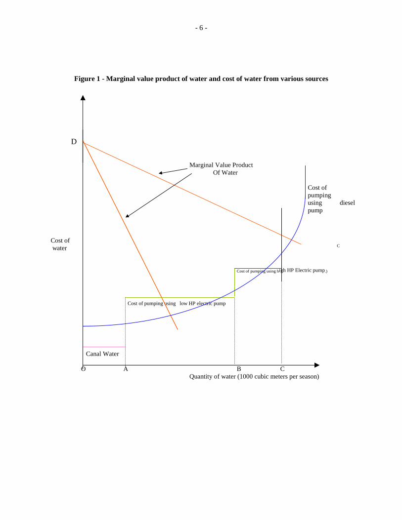
B. Cost Structure of Alternative Irrigation Options 1.9 In this subsection, the costs and benefits of irrigation through electric pumps are compared to other irrigation options available to farmers. In most regions where surface water is available for irrigation purposes, it is the lowest cost alternative for irrigation (see Fig. 1). The costs associated with canal irrigation include the cost of digging and maintaining field channels and a highly subsidized payment to the irrigation department in terms of crop and area cultivated. However, there are quotas or other kinds of quantitative limits on the total amount of canal water that is available per season. Farmers also have very little flexibility with respect to the timing of supply because a fixed rotation schedule is followed.

- 6 -

Figure 1 - Marginal value product of water and cost of water from various sources

D Marginal Value Product Of Water Cost of

pumping using diesel pump

Cost of water C

Cost of pumping using high HP Electric pump.)

Cost of pumping using low HP electric pump

Canal Water O A B C Quantity of water (1000 cubic meters per season)

- 7 -

1.10 Thus in most cases, farmers use whatever surface water is available and supplement it with other sources. Investment in an irrigation well is a large and risky investment in most areas, and particularly so, in the hard rock areas of Andhra Pradesh. As pointed out earlier, in most areas a fixed tariff per unit of installed capacity is charged irrespective of the volume of water pumped out. Thus, the variable costs associated with electric pump operation are very low and consist primarily of cost incurred in motor repair and maintenance. As opposed to this, the variable cost associated with operation of diesel pumps are much higher (as shown by the much steeper slope of the diesel cost line in Fig. 1). 1.11 Given the poor availability and reliability of electricity supply, however, diesel pumps are often used as a backup strategy to meet the shortfalls in supply of electric power. In addition, in some areas where canal is the main source of irrigation but a supplemental source is needed, farmers may prefer to use diesel pumps rather than electric pumps if groundwater table is high. This is because for electric pumps they have to pay a fixed tariff irrespective of use, whereas for a diesel pump they pay per unit of diesel consumption. Thus a diesel pump may be more profitable at low levels of consumption. 1.12 For those farmers who do not own wells, use of canal water or purchase of water from well-owners are the only two options for irrigation. Evidence from several studies suggests that markets for water tend to be very thin and fragmented for several reasons (Shah, 1993 provides a survey). First, because of the physical costs of transporting water over large distances, transactions in groundwater tend to be limited between neighboring farmers. Second, farmers in a given region generally grow very similar crops and hence their demand for water tends to be synchronous. Given this synchronicity in demand and uncertainty regarding the dynamics of groundwater stock, transaction costs are generally quite high and so water markets tend to be very thin. Third, in many areas, there is also an underlying social belief that water is a natural, common pool resource that belongs to everyone and therefore charging a price for it is immoral (Wood, Aggarwal). In the attitude survey conducted in Haryana, it was found that of the 600 pumpset owners covered under the survey, only 3 per cent (around 22 farmers) reported selling water to other farmers. Thus for those farmers who do not own wells, the options for irrigation are rather limited. 1.13 Thus to sum up, from a farmer’s perspective, in areas where canal water is available, it is the lowest cost alternative for irrigation. However, there are quotas and farmers have very little control on the timing of irrigation applications from canal water. For those farmers who can invest in wells, electricity is much less costlier than diesel as an energy source. However, given the poor availability and quality of electricity supply, farmers often use diesel pumps as a backup or a supplemental source of power. The growing use of diesel pumps is a rough indicator of the fact that the current supply of electricity is inadequate for the needs of the farmers and that they are willing to pay a much higher price for additional and more reliable supply. 1.14 From the society’s perspective, since electricity supply is not priced at its true scarcity value, there is a loss in overall social efficiency. Moreover, with a flat rate there are very limited incentives at the margin to conserve either water or power, through the use of more efficient pumps or water conserving technologies. As discussed earlier, uncertainty about availability of electricity supply leads to production losses and forces farmers to adopt various kinds of coping strategies which are highly inefficient, such as the use of diesel operated tractors to pump water when electricity is not available. All this raises the question of whether at the margin it is more efficient for the utility to improve the reliability of supply and charge a somewhat higher price or to let the farmers evolve their own private mechanisms to deal with this situation. 1.15 In this context, it is also worth noting that in the present situation where there is no explicit regulation of groundwater pumping, the allocative effects of electricity rates on water extraction are also very important. Although it is true that the scarce value of the groundwater resource can be better addressed by other more direct policies such as pumping limits and pump spacing, the potential for

- 8 -

electricity rate structures to encourage or discourage groundwater extraction cannot be ignored. Shah (1992) conducted a survey of studies on groundwater use in areas where a switch was made from per unit to flat tariffs in the late 1970s/early 1980s. His main conclusion was that this switch resulted in an increase of 40 to 60% in pumping of water by existing well owners. This finding reinforces the need for revisions in the current tariff structure, particularly in areas where water table is declining rapidly or where there is an imminent danger of saline intrusion.

C. Proposed Policy Reforms

1.16 As discussed above, the current situation regarding electricity supply results in low revenues for the utility and high real costs borne by the farmers and the society. Thus, the overall result is a situation where all the major stakeholders find themselves in a situation of a “low equilibrium trap”. This calls for the need for policy reforms which can help the economy emerge out of this trap. 1.17 The policy reform process proposed in this study consists of a combination of some or all of the following changes: 1.18 Increase in number of hours for which electricity is supplied to the agricultural sector. Improvements in reliability of supply: reduction in the frequency and duration of unscheduled power cuts. An important component of policy here is the reduction in the frequency of transformer burnouts and time taken to repair it. Improvements in quality of supply. Reduction in magnitude (how high or low compared to the standard agreed by the utility), frequency and duration of voltage fluctuations Increase in tariff : This could take the form of increase in the current fixed rates charged per horsepower of pump or a move towards pro-rata tariff with installation of meters. 1.19 An important objective of this project is to estimate the impact of these policies on input (in particular, water and electricity) demands, cropping patterns and farm costs and incomes. The purpose is to estimate these impacts both over the short run (when the capital stock, particularly in the form of installed irrigation capacity is held constant) and the medium to long run (when capital stock is allowed to adjust). The sequencing and pace of the reform process is likely to be very important. Thus for instance, increasing the rates without improvements in quality of supply is not likely to be politically feasible. Hence one of the objectives of this study is to shed light on these aspects by simulating the impact under alternative policy reform scenarios as shown in Figure 2.

Figure 2 - Policy matrix showing alternative reform scenarios

Scenario Policy

Option 1 2 3 4 5 6?

Increase tariff X X X X X

Increase hours of supply X X

Reduce power interruptions X X X

Reduce voltage fluctuations X X

Others?

- 9 -

D. Review of Alternative Approaches and Justification for Proposed Approach

1.20 As discussed above, the main purpose of this study is to evaluate the impact of policy reforms in the power sector on agriculture. The study has two broad components. The first one relates to the micro aspects (pertaining to farm level behavior) and the other relates to the macro aspects (at the region or state level). For now only the micro level is complete. This analysis is conducted within a partial equilibrium framework and the focus here is to examine the impact of policy reforms on costs of production, yields, cropping patterns, demand for electricity and farm incomes for different categories of farmers classified as marginal, small, medium and large. 1.21 To evaluate the impact of policy reform quantitatively at the micro level, an econometric model based on data on observed choices of farmers in the current situation is used. This predicts what farmers are likely to do when the policy change occurs. 1.22 Another method would have been to use a contingent valuation survey (CV) elicits farmer’s responses and willingness to pay for the changes in policiy. The advantage of the CV approach is that it can in eliciting expected responses and willingness to pay for any change towards a given hypothetical situation. However, earlier studies have pointed out that responses are very sensitive to the manner in which the questions are phrased and upon the timing of such a survey vis-a-vis the household’s recent outage experience (Sanghvi). Given these difficulties with CV surveys, we propose to use an econometric model to estimate the impact of policy reforms. 1.23 In examining the impact of policy reforms it is often useful to distinguish between the short and the medium run. In the ensuing analysis on the micro aspects, it is assumed that the short run is the period in which the capital stock representing the technology imbedded in the production process, remains constant. On the other hand, in the medium run, the capital stock is allowed to respond to changes in conditions of electricity supply. However, over the medium run it is assumed that everything else in the farm economy, such as output/ input prices and the overall regulatory framework with respect to the agricultural sector , remains constant.1 Thus for instance, in the short run, farmers may respond to unexpected power outages by say, rescheduling production activities and changing the allocation of variable inputs. In the medium run (a period of about 4 to 6years), if it is expected that these power outages will continue then farmers may shift to alternative fuel source (say, shift to use of diesel), install larger capacity pumps or install backup generation capability. In his survey of the literature on optimal electricity supply reliability, Sanghvi points out that almost the entire literature so far has focused on short-run cost of power outages. As he argues, in the medium run, with shift in the capital stock the demand curve itself can shift. Since the policy changes being proposed are likely to result in major changes in the supply of electricity, assuming the demand curve to remain constant would assume away the essence of the problem at hand. An important objective of the present study is to examine how farmers respond to the current problem in electricity supply and to assess the cost of the backup technologies that they invest in. Thus the model has two related parts. The first part consist of estimating the input and output elasticity in the short run, keeping the technology as constant. The second part models the choice of technology in the medium run. 1.24 To model the choice of technology, it is important to consider the entire spectrum of irrigation options currently in use in the selected states. Thus the sample used for the study includes not only the users of electric pumps but the entire farming population ( diesel pumpset owners, rainfed, canal and water purchasers). This is important for several reasons. Firstly, restricting the sample to only electric

1 This is the main difference between medium and long run. Long run effects have not been analyzed right now.

- 10 -

users would result in selectivity bias in the estimates derived from the econometric model. Secondly, it is necessary to estimate how cropping patterns, input allocations, yields and incomes differ between those who own wells with electric pumps as compared to all other categories of farmers. In particular, the returns currently associated with use of electricity in pumping groundwater are compared with other options. Some earlier studies have compared input intensities and yields between canal and groundwater irrigated areas. However, very few of these analysis have been conducted within a multivariate regression framework and so it is difficult to assess the extent to which the differences found in input intensities and yields can be uniquely attributed to the use of groundwater (see Dhawan, Shah for a survey). Thirdly, the impact of policy reforms on changes in irrigation technology in the short to medium run need assessing. It is likely, for instance, that some non-well owners might decide to invest in electric pumps or buy water from electric pump owners as a consequence of the policy change. Thus it is important to establish what factors determine farmer’s choice of technology and how. 1.25 The data to be used for this study was obtained through a farm household level survey for the agricultural year 1999-2000 in the states of Haryana and Andhra Pradesh. Details of the sampling design for the present study are given inpart II. Using this data, the econometric model described in section F was developed. Estimates derived from this econometric model were used to do a partial equilibrium analysis of policy reforms. An important advantage of the partial equilibrium approach is its empirical simplicity and also the fact that the first round effects are, in general, an acceptable first-order approximation of the total effects (Sadoulet and deJanvry). However, it is important to keep in mind that the partial equilibrium analysis does not take into account several important effects such as the income and cost changes that might shift the demand and supply curves and the interaction across markets with products or factors that are close substitutes or complements in consumption or production. For example, it is likely that policy reforms that would affect agricultural production and hence lead to a change in the prices of major crops produced in these states. The partial equilibrium analysis does not take into account this second round effect. To take into account such indirect effects, the analysis of policy reform would possibly be extended to a general equilibrium framework. 1.26 In the next section, the set of questions that need to be addressed are listed. This provides an overall perspective and is followed by a detailed discussion on the methodology.

E. Questions to be addressed

Part I: Analysis of the current situation with subsidized fixed tariffs and rationed supply of electricity

A. What are the different sources of irrigation (both surface and groundwater) used by different categories of farmers?

B. What are the different technologies used for pumping groundwater (Type of well, depth of well, type of pump, source of power, use of backup strategies etc.)

For the purposes of this study, four broad categories of technological options for irrigation are distinguished. 1) Use of electric pumps to withdraw groundwater from own well 2) Use of electric pumps (with back up strategies such as use of diesel pump or tractor) to withdraw

groundwater from own well 3) Use of diesel pumps to withdraw groundwater from own well 4) Use of neither electricity nor diesel for irrigation. This includes rainfed farmers and those that rely

solely on surface water sources and/or purchase of water from neighboring well owners.

C. What are the direct and indirect costs (such as costs of motor burnouts in case of electric pump users) associated with the adoption and use of the above technological options?

- 11 -

D. What are the cropping patterns, input use intensities and yields associated with each of these options?

E. What are the input demand (including demand for power) and output supply elasticities associated with these different options?

F. What are the various farm and village-specific characteristics that determine the choice of technology used for pumping groundwater?

G. What is the pattern of electricity use by electric well owners? In particular, for each crop, what are the peak and off peak periods of demand for pumped water and hence for electricity?

H. How do farmers perceive the different qualitative aspects of supply (i.e. reliability, flexibility in supply) associated with the current supply of electricity?

I. What kind of coping strategies are currently being used by farmers to deal with problems of electricity supply? What are the costs of adopting these strategies?

J. For electric well owners who do not have any backup strategies, what is the estimated loss in production in the short run?

K. Do well owners also sell water to neighboring farmers? If so, how much water is contracted out and what are the terms of the contract (fixed price or crop share)? How are the terms of these contracts framed in order to deal with uncertainties in electricity supply? Do the terms of the contract differ for water purchased from electric pump owners as opposed to diesel pump owners?

Part II: Partial equilibrium analysis of policy changes

A. What is the impact of alternative policy changes on technology used for pumping: (shift to diesel pumps or pumps with higher efficiency, use of water conserving methods of irrigation, use of coping strategies), cropping patterns, total demand for electricity, total amount of groundwater withdrawn, yields, input intensities, costs and incomes. In particular, what is the impact of policy reforms on the small and marginal farmers?

B. What is the willingness to pay for an extra hour of electricity at prevailing quality levels?

C. What is the willingness to pay for an improvement in reliability and quality of electric supply? The conceptual model underlying the analysis of the above questions in outlined in the next section.

- 12 -

F. The Conceptual Model

1.27 Basic assumptions

Production function Consider an agricultural production function given by

Y = f(W, X; Z, θ ) (1)

where W = water input X = vector of variable inputs employed in production such as land, seeds, labor, manure, fertilizers, pesticides, hours of tractor and machine use Z = farm specific characteristics θ = random factor denoting the effect of weather (rainfall, temperature etc.)

We assume that f(.) is twice continuously differentiable and concave in all of its arguments. In addition we assume that fW ! ∞ as W ! 0, and similarly for X. Water input, W, in the production process is subject to the following constraint

W ≤ WR + Wc + We + Wd (2)

where WR is the amount of rain water, WC is the exogenously allocated amount of canal water, We is the amount of water pumped using own electric pumps and Wd is the amount of water pumped using own diesel pumps2. To begin with, we assume that there is no buying or selling of water. This assumption is relaxed later on. Pumping technology Water from electric pumps is pumped using the following technology

We = We (he, HPe, E, Vavg , G) (3) where he denotes hours of pumping, HPe is the horsepower of the pump, E is efficiency of pump, Vavg is average voltage during season, G denotes characteristics of groundwater aquifer (e.g. depth of water table and rate of natural recharge). We is assumed to be increasing in he, HPe, E and Vavg.

Similarly, water from diesel pumps is pumped using the following technology

Wd = Wd (hd, HPd, E; G) (4)

where hd denotes hours of pumping and HPd is the horsepower of the diesel pump. Wd is assumed to be increasing in hd , HPd, and E. Electricity rationing Electricity is available for only a limited number of hours during the season given by

Her = AHse (5)

2 We assume here that water used through these alternative sources is equivalent in terms of their effect on production. It might be more realistic to put different weights on these different sources with the highest weight on water pumped by diesel pumps because it is “on demand” while the lowest weight is put on rain water since the farmer has no control over its application

- 13 -

where Hse is the scheduled hours of supply (known before the start of the season) and A is the availability index defined as

A = Hours of actual supply/ hours of scheduled supply (6)

We assume the uncertainty about A is resolved during the course of the season. Groundwater availability There is an upper bound on the amount of total groundwater that can be withdrawn through electric and diesel pumps. This upper bound W0 is given by factors such as: aquifer characteristics G, rainfall during the season R, availability of canal water, Wc and density of wells, D, in the cluster W0 = W0( G, WR, Wc, D) (7) Costs of pumped and canal water a) Fixed costs of pumped water: In order to extract groundwater, there are sunk costs of digging the well

and installing the pumps. Let Qd (HPd) and Qe(HPe) be the sunk costs of installing diesel and electric pumps of horsepower HPd and HPe respectively3. In case of electric pumps, Qe(HPe) includes, in addition, a one-time electricity connection charge. In most regions, a flat tariff of T(HPe) is charged on electric pumps which has to be paid every season

b) Variable costs of pumped water: In addition to these sunk costs, we assume that there is a constant per

hour cost of pumping with a diesel pump qd, which is a function of the horsepower of the pump and is given by

qd = pd δ(HPd) + md (HPd,, Fd) (8)

where pd is price of diesel and δ(HPd) is the consumption of diesel per hour by a pump of horsepower HPd. md denotes the non-fuel cost of operation of diesel pumps and relates to expenses incurred in oiling, replacement of bearings etc. These non-fuel costs of operation are a function of the horsepower of the pump and other characteristics such as age and brand, denoted by Fd.

Similarly for electric pumps we assume that there is a constant per hour cost of pumping, qe. It includes fuel cost (in cases where a metered tariff is in place) and the non-fuel costs of operation of pumps and relates to expenses incurred in oiling, replacement of bearings and motor rewindings due to motor burnouts. Apart from normal wear and tear, motor burnouts often arise because of voltage fluctuations. Therefore, the per hour cost of operation of electric pumps, qe can be given as

qe = peHPe + m(HPe, Fe, Vfluc, ,) (9) where pe is price of electricity consumption per HP per hour(for metered pumps), Vfluc is an index of voltage fluctuations during the season and Fe is a vector of pump specific characteristics such as age and brand 4. In general, the marginal cost of a unit of water pumped through electric pumps is much smaller than that through diesel pumps. This is so even with respect to farmers who currently pay on the basis of metered tariff, because the use of electricity in agriculture is more heavily subsidized than the use of diesel (see figure 2).

3 This cost includes the cost of digging a well, installing a motor and applying for an electricity connection ( in case of electric pumps). 4 We are still working on defining these indices using the available data.

- 14 -

In comparison to the costs of pumped water given above, the total costs of canal water (which includes costs of digging and maintaining field channels plus the seasonal tariff) are very low. Canal water is available in only a few regions, wherein, farmers have an exogenously given quota denoted as Wc and are charged a seasonal tariff of PcWc.

Prices: prices of output and variable inputs (other than water) are denoted by PQ and PX respectively.

1.28 Farm household’s optimization problem: two stage formulation

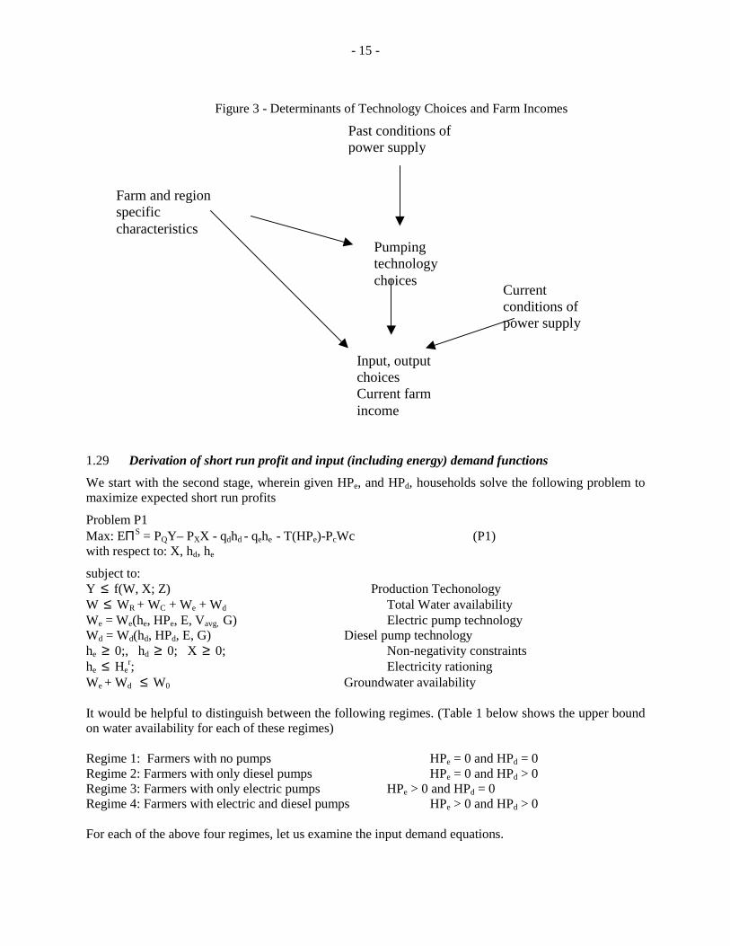
The farm household’s decision problem has two stages: First, households choose the irrigation technology. Here we will consider the main choice variables to be the installed electric and diesel pumping capacity, HPe and HPd, respectively. Next, households observe the amount of rainfall, availability of canal water and conditions of electricity supply (i.e. incidence of unscheduled cuts, and the duration and magnitude of voltage fluctuations). They then choose the level of application of variable inputs (X) and hours of pumping for electric and diesel pumps ( he and hd, respectively)5. The two stage optimization problem presented in this section is summarized in Figure 3.

5 In the presentation of the optimization problem we assume that households are not credit constrained. In a later section we discuss the implications of credit constraints.

- 15 -

Figure 3 - Determinants of Technology Choices and Farm Incomes

1.29 Derivation of short run profit and input (including energy) demand functions

We start with the second stage, wherein given HPe, and HPd, households solve the following problem to maximize expected short run profits

Problem P1 Max: EΠS = PQY– PXX - qdhd - qehe - T(HPe)-PcWc (P1) with respect to: X, hd, he

subject to: Y ≤ f(W, X; Z) Production Techonology W ≤ WR + WC + We + Wd Total Water availability We = We(he, HPe, E, Vavg, G) Electric pump technology Wd = Wd(hd, HPd, E, G) Diesel pump technology he ≥ 0;, hd ≥ 0; X ≥ 0; Non-negativity constraints he ≤ He

r; Electricity rationing We + Wd ≤ W0 Groundwater availability It would be helpful to distinguish between the following regimes. (Table 1 below shows the upper bound on water availability for each of these regimes) Regime 1: Farmers with no pumps HPe = 0 and HPd = 0 Regime 2: Farmers with only diesel pumps HPe = 0 and HPd > 0 Regime 3: Farmers with only electric pumps HPe > 0 and HPd = 0 Regime 4: Farmers with electric and diesel pumps HPe > 0 and HPd > 0 For each of the above four regimes, let us examine the input demand equations.

Past conditions of power supply

Pumping technology choices

Current conditions of power supply

Farm and region specific characteristics

Input, output choices Current farm income

- 16 -

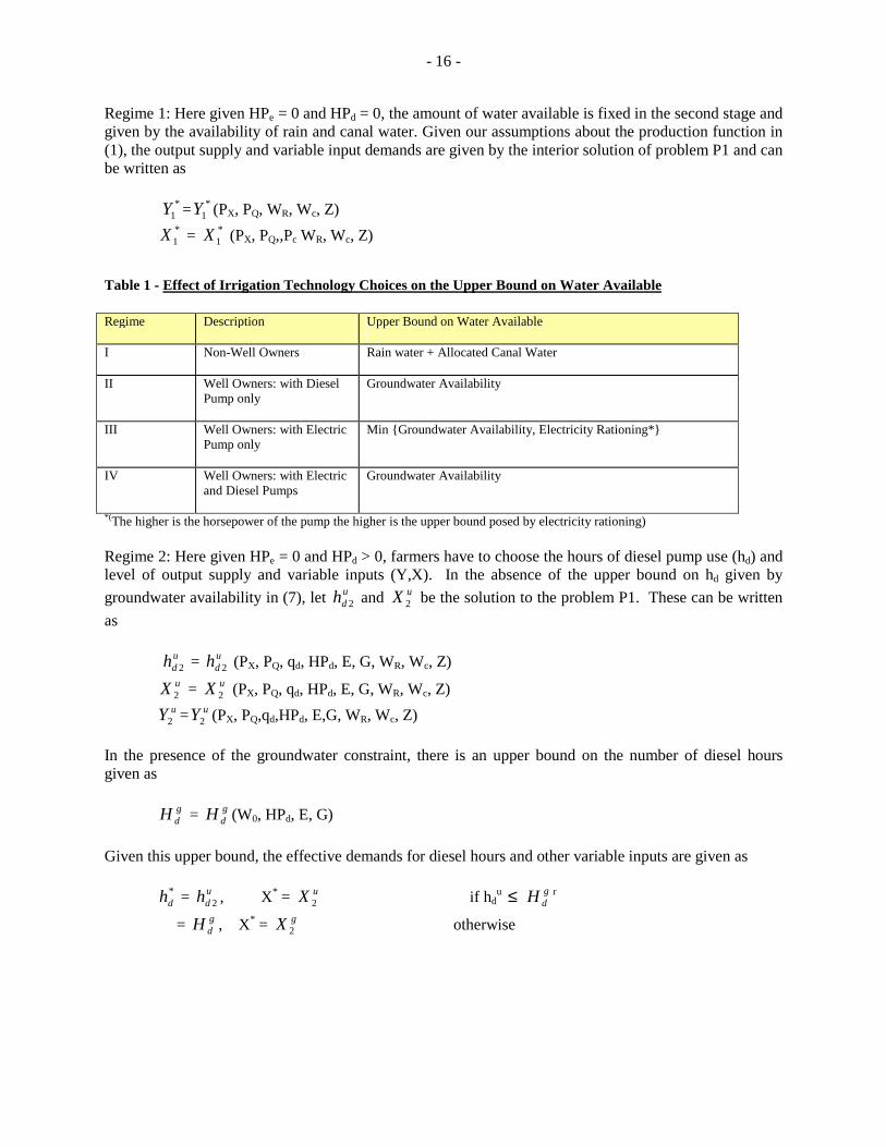
Regime 1: Here given HPe = 0 and HPd = 0, the amount of water available is fixed in the second stage and given by the availability of rain and canal water. Given our assumptions about the production function in (1), the output supply and variable input demands are given by the interior solution of problem P1 and can be written as *

1Y = *1Y (PX, PQ, WR, Wc, Z)

*1X = *

1X (PX, PQ,,Pc WR, Wc, Z) Table 1 - Effect of Irrigation Technology Choices on the Upper Bound on Water Available Regime Description Upper Bound on Water Available

I

Non-Well Owners Rain water + Allocated Canal Water

II Well Owners: with Diesel Pump only

Groundwater Availability

III Well Owners: with Electric Pump only

Min {Groundwater Availability, Electricity Rationing*}

IV Well Owners: with Electric and Diesel Pumps

Groundwater Availability

*(The higher is the horsepower of the pump the higher is the upper bound posed by electricity rationing) Regime 2: Here given HPe = 0 and HPd > 0, farmers have to choose the hours of diesel pump use (hd) and level of output supply and variable inputs (Y,X). In the absence of the upper bound on hd given by groundwater availability in (7), let u

dh 2 and uX 2 be the solution to the problem P1. These can be written as u

dh 2 = udh 2 (PX, PQ, qd, HPd, E, G, WR, Wc, Z)

uX 2 = uX 2 (PX, PQ, qd, HPd, E, G, WR, Wc, Z) uY2 = uY2 (PX, PQ,qd,HPd, E,G, WR, Wc, Z)

In the presence of the groundwater constraint, there is an upper bound on the number of diesel hours given as g

dH = gdH (W0, HPd, E, G)

Given this upper bound, the effective demands for diesel hours and other variable inputs are given as *

dh = udh 2 , X* = uX 2 if hd

u ≤ gdH r

= gdH , X* = gX 2 otherwise

- 17 -

where gX 2 is the solution to the problem P1 when hd is fixed at gdH 6.

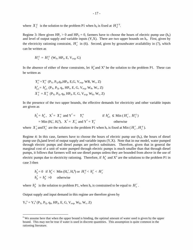
Regime 3: Here given HPe > 0 and HPd = 0, farmers have to choose the hours of electric pump use (he) and level of output supply and variable inputs (Y,X). There are two upper bounds on he. First, given by the electricity rationing constraint, r

eH in (6). Second, given by groundwater availability in (7), which can be written as g

eH = geH (W0, HPe, E, Vavg, G)

In the absence of either of these constraints, let e

uh and Xu be the solution to the problem P1. These can be written as uY3 = uY3 (PX, PQ,qd,HPd, E,G, Vavg, WR, Wc, Z)

euh 3 = e

uh 3 (PX, PQ, qe, HPe, E, G, Vavg, WR, Wc, Z)

uX 3 = uX 3 (PX, PQ, qd, HPd, E, G, Vavg, WR, Wc, Z) In the presence of the two upper bounds, the effective demands for electricity and other variable inputs are given as *

uh = euh , X* = uX 3 and Y* = uY3 if e

uh 3 ≤ Min ( reH , g

eH )

= Min (Her, He

g), X* = rX 3 and Y* = rY3 otherwise

where rX 3 and rY3 are the solution to the problem P1 when he is fixed at Min ( reH , g

eH ). Regime 4: In this case, farmers have to choose the hours of electric pump use (he), the hours of diesel pump use (hd)and level of output supply and variable inputs (Y,X). Note that in our model, water pumped through electric pumps and diesel pumps are perfect substitutes. Therefore, given that in general the marginal cost of a unit of water pumped through electric pumps is much smaller than that through diesel pumps, it follows that farmers will not use diesel pumps unless they are bounded from above in the use of electric pumps due to electricity rationing. Therefore, if e

uh and Xu are the solutions to the problem P1 in case 3 then *

dh = 0 if euh < Min (He

r, Heg) or g

eH < euh < r

eH

*dh = u

dh >0 otherwise

where udh is the solution to problem P1, when he is constrained to be equal to r

eH . Output supply and input demand in this regime are therefore given by Y4

u = Y4u (PX, PQ, qd, HPd, E, G, Vavg, WR, Wc, Z)

6 We assume here that when the upper bound is binding, the optimal amount of water used is given by the upper bound. This may not be true if water is used in discrete quantities. This assumption is quite common in the rationing literature.

- 18 -

X4u = X4

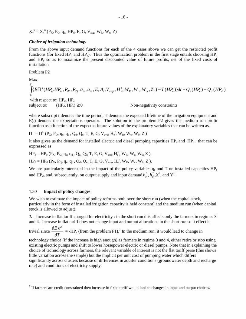
u (PX, PQ, qd, HPd, E, G, Vavg, WR, Wc, Z) Choice of irrigation technology From the above input demand functions for each of the 4 cases above we can get the restricted profit functions (for fixed HPd and HPe). Thus the optimization problem in the first stage entails choosing HPd and HPe so as to maximize the present discounted value of future profits, net of the fixed costs of installation

Problem P2

Max

)()()}(),,,,,,,,,,,,({0

ddee

T

etotctRtretavgtttdtetQtXtetd

st HPQHPQdtHPTZWWWHVAEqqPPHPHPE −−−Π∫

with respect to: HPd, HPe subject to: (HPd, HPe) ≥ 0 Non-negativity constraints where subscript t denotes the time period, T denotes the expected lifetime of the irrigation equipment and E(.) denotes the expectations operator. The solution to the problem P2 gives the medium run profit function as a function of the expected future values of the explanatory variables that can be written as

ΠL = ΠL (PX, PQ, qe, qd , Qd, Qe, T, E, G, Vavg, Her, WR, Wc, W0, Z )

It also gives us the demand for installed electric and diesel pumping capacities HPe and HPd, that can be expressed as

HPe = HPe (PX, PQ, qe, qd , Qd, Qe, T, E, G, Vavg, Her, WR, Wc, W0, Z ),

HPd = HPd (PX, PQ, qe, qd , Qd, Qe, T, E, G, Vavg, Her, WR, Wc, W0, Z ).

We are particularly interested in the impact of the policy variables qe and T on installed capacities HPe and HPd, and, subsequently, on output supply and input demand *

eh , *dh ,X*, and Y*.

1.30 Impact of policy changes We wish to estimate the impact of policy reforms both over the short run (when the capital stock, particularly in the form of installed irrigation capacity is held constant) and the medium run (when capital stock is allowed to adjust).

1. Increase in flat tariff charged for electricity : in the short run this affects only the farmers in regimes 3 and 4. Increase in flat tariff does not change input and output allocations in the short run so it effect is

trivial since T

E s

∂∂ π

= -HPe (from the problem P1).7 In the medium run, it would lead to change in

technology choice (if the increase is high enough) as farmers in regime 3 and 4, either retire or stop using existing electric pumps and shift to lower horsepower electric or diesel pumps. Note that in explaining the choice of technology across farmers, the relevant variable of interest is not the flat tariff perse (this shows little variation across the sample) but the implicit per unit cost of pumping water which differs significantly across clusters because of differences in aquifer conditions (groundwater depth and recharge rate) and conditions of electricity supply.

7 If farmers are credit constrained then increase in fixed tariff would lead to changes in input and output choices.

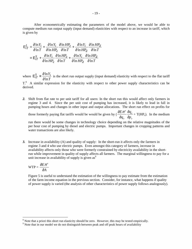
- 19 -

After econometrically estimating the parameters of the model above, we would be able to compute medium run output supply (input demand) elasticities with respect to an increase in tariff, which is given by

THP

HPY

THP

HPY

THP

HPY

THP

HPY

TY

d

d

ie

e

iSiT

d

d

ie

e

iiLiT

lnln

lnln

lnln

lnln

lnln

lnln

lnln

lnln

lnln

∂∂

∂∂+

∂∂

∂∂+Ε=

∂∂

∂∂+

∂∂

∂∂+

∂∂=Ε

where TYiS

iT lnln

∂∂≡Ε is the short run output supply (input demand) elasticity with respect to the flat tariff

T.8 A similar expression for the elasticity with respect to other power supply characteristics can be derived.

2. Shift from flat rate to per unit tariff for all users: In the short run this would affect only farmers in regime 3 and 4. Since the per unit cost of pumping has increased, it is likely to lead in fall in pumping hours and changes in other input and output allocations. The short run effect on profits for

those formerly paying flat tariffs would be would be given by (e

e

e

s

pq

qE

∂∂

∂∂ π

+ T(HPe). In the medium

run there would be some changes in technology choice depending on the relative magnitudes of the per hour cost of pumping by diesel and electric pumps. Important changes in cropping patterns and water transactions are also likely.

3. Increase in availability (A) and quality of supply: In the short-run it affects only the farmers in regime 3 and 4 who use electric pumps. Even amongst this category of farmers, increase in availability affects only those who were formerly constrained by electricity availability in the short-run while improvement in quality of supply affects all farmers. The marginal willingness to pay for a unit increase in availability of supply is given as9

WTP = A

E s

∂∂ π

Figure 5 is useful to understand the estimation of the willingness to pay estimate from the estimation of the farm income equation in the previous section. Consider, for instance, what happens if quality of power supply is varied (the analysis of other characteristics of power supply follows analogously).

8 Note that a priori this short run elasticity should be zero. However, this may be tested empirically. 9 Note that in our model we do not distinguish between peak and off peak hours of availability

- 20 -

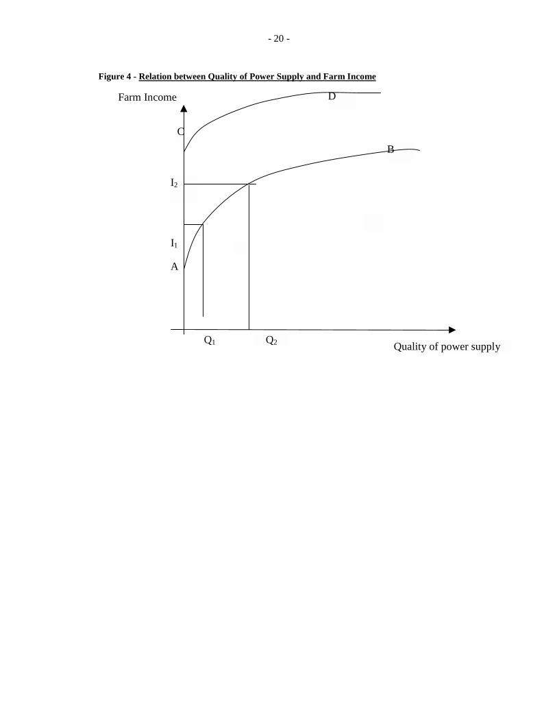
Figure 4 - Relation between Quality of Power Supply and Farm Income

Farm Income D

C B

I2

I1

A

Q1 Q2 Quality of power supply

- 21 -

In Figure 4, quality of power supply is shown along the horizontal axis and farm income is shown along the vertical axis. The curve AB shows the relation between quality of power supply and farm incomes, assuming that everything else remains constant. Suppose that in the initial situation, quality of power supply is at point Q1 and thus farm income is I1. If quality of supply increases to point Q2 then income would increase to I2 as show in the figure. The increase in income, I2 –I1 can be interpreted as the willingness to pay for increase in quality of supply from Q2 to Q1. For a unit change in quality, the coefficient on the quality variable in table 6 gives an estimate of how much incomes increase in the short run and thus how much tariffs can be increased without making farmers any worse off. Note the effect of electricity supply characteristics may be different across farmers depending on the amount of land they own. Thus for instance, for larger farmers, the curve showing the relation between farm income and availability might be much flatter (shown as curve CD in figure 5) than for the smaller farmers (shown as curve AB in figure 5). If this is true then this implies that smaller farmers gain more than the larger farmers do with any given improvement in supply conditions.

In the medium run, increase in scheduled hours of supply will also affect technology choices as one might expect some farmers in regimes 1 and 2 to adopt electric pumps, if the tariff structure remains the same. Those already using electric pumps might shift to lower horsepower pumps and feel less compelled to use backups (such as diesel pumps and generators), if the tariff structure remains the same.

- 22 -

Appendix I.1

The Econometric model In the previous section, we classified farmers into four regimes depending on their installed irrigation capacity and showed how the upper bound on water availability is dependent on the regime to which they belong. To allow for the possibility that the effect of the various explanatory variables may be different across these different regimes, it would be useful to estimate a separate short-run profit function for each regime, r, in the following way: Πri

s = Mriβr + εri r = 1, 2 …4 (10) where the subsrcipt i indexes the observation number (i = 1,2 …..n), Πr

s is the short-run profit function under regime r, Mr is the set of exogenous explanatory variables under regime r (based on the derivation of the short-run profit function in section I above) and εr is the error term associated with the rth regime. Several points need to be noted in the estimation of the above equation. First note that the choice of regime is endogenous so that estimation of above equation by OLS would result in inconsistent estimates. Note that it follows from our theoretical model that the individual chooses to be in regime r if the expected medium-run profits from this regime are at least as large as that under the other regimes. To formalize this idea, let I denote a polychotomous variable that takes on the values 1 to 4. We observe I = r if the rth regime is chosen I = r iff *

rI > Max *jI (j =1, 2, ..4; j ≠ r) (11)

where, *

rI denotes the expected medium run profit from choosing the rth regime and is given as *

riI = Nriγ + ηri i = 1,2 …..n (12) where Nr is the set of exogenous explanatory variables (based on the derivation of the medium-run profit function in section I above). To estimate the model given by (10) to (12) we need to make assumptions regarding the distribution of the error terms. We assume that εr are distributed as N (0, σ2

r). We also assume that ηr (r=1, 2, ..4) are independently and identically distributed with type I extreme value distribution with cumulative distribution function F(ηr < c) = exp [- exp (-c)] Let ur = Max *

rI - ηr (j =1, 2, ..4; j ≠ r) It then follows that I = r iff ur < Nrγ Therefore, for each choice r, our model now becomes Πr

s = Mrβr + εr

- 23 -

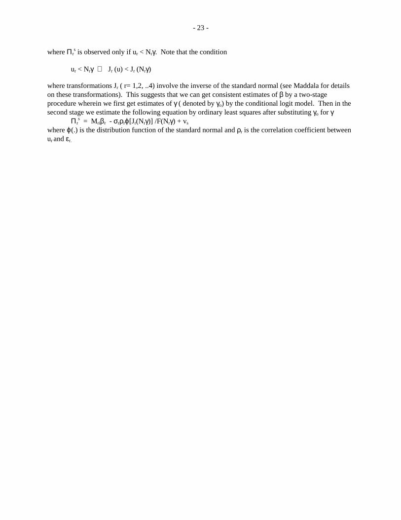
where Πrs is observed only if ur < Nrγ. Note that the condition

ur < Nrγ ⇔ Jr (u) < Jr (Nrγ) where transformations Jr ( r= 1,2, ..4) involve the inverse of the standard normal (see Maddala for details on these transformations). This suggests that we can get consistent estimates of β by a two-stage procedure wherein we first get estimates of γ ( denoted by γo) by the conditional logit model. Then in the second stage we estimate the following equation by ordinary least squares after substituting γo for γ

Πrs = Mriβr - σrρrϕ[Jr(Nrγ)] /F(Nrγ) + vs

where ϕ(.) is the distribution function of the standard normal and ρr is the correlation coefficient between ur and εr.

- 24 -

Appendix II.2

Availability and Reliability of Power Supply at Feeder Level Under a detailed study carried out on four sample feeders in Haryana, using electronic meters with data logging facilities to record information on voltage and currents, indices related to availability and reliability of availability have been developed. This have been defined as regards to the duration and characteristics of the three-phase power supplied to farmer. These indices could not be used in the econometric model because the electronic feeders covered only 4 feeders. However, the daily readings taken from these electronic meters serve as a more objective measure of power supply conditions and have been used to validate and complement the data collected on the basis of farmers’ recall. Availability Index The Availability Index, is defined as the number of hours in a day during which the 3 phase supply is made available to farmers with respect to the corresponding scheduled number of hours Total hours of three phase power supply Availability Index = ----------------------------------------------------------------------------- Scheduled number of hours of three phase power supply Thus, if during the three phase supply, there is no significant difference between the actual number of hours of three phase supply and the scheduled number of hours period announced by the utility, the Availability Index would be equal to 1. The index would therefore reflect the overall availability of three phase supply during the day, irrespective of the time of availability, and assuming that the farmer can operate the pumps at any time. The higher the availability index the greater would be the number of hours of supply available to the farmer. Assuming 8 hours per day as the scheduled number of hours of three phase supply, the Availability Index will vary from a minimum value of zero when no three phase power is supplied during the day to a maximum value of 3 when the three phase supply is available for 24 hours. However, it should be emphasized that the index reflects availability from the feeder side, as farmers can’t have a higher availability than reflected by the index. In case of a local outage such as a failure of a distribution transformer, farmers could, however, have a lower level of availability. Reliability of Availability index Reliability of Availability index is defined as the ratio between the number of hours during which the power supply was available during the scheduled period of supply and the scheduled number of hours of power supply by utilities. Hours of three-phase power supply during scheduled period Reliability of Availability Index = ---------------------------------------------------------------------------- * 100 Scheduled number of three phase power supply This index attempts to capture the importance attributed by farmers to the reliability of availability of power supply during the scheduled period, particularly during peak irrigation times. The index also indicates the extent to which a particular curtailment policy is being implemented by the utility . The Reliability of Availability Index would vary between a minimum value of zero when no power is supplied during the scheduled hours of supply to a maximum of 1 when power is available for the entire scheduled duration of supply.

- 25 -

PART II

A. Sampling and Survey Procedures Metering and survey approaches 1.31 Power supply to agriculture in a state is primarily used for running of pumpsets. However, only a small fraction of pumpsets is metered (and even then, not very reliably) while the rest are unmetered. Power supply to pumpsets in the former category is charged as per the meter readings and prevailing agricultural tariff (subject to a minimum charge) while for unmetered pumpsets, it is charged on a flat rate. There is thus no objective method of determining the actual consumption of power in agriculture in a state. 1.32 Since pumpsets are by and large not metered, the procedure adopted by the state utility for assessing the power consumption in agriculture is to determine the consumption of power for industrial, commercial and domestic sectors (since consumers in all these categories are metered) and subtract the aggregate consumption of these sectors from the total supply (after allowing for acceptable level of transmission and distribution (T&D) losses) to obtain the consumption in agriculture. In practice, losses on account of illegal/unauthorized use and thefts/pilferage (non technical losses) in addition to T&D losses in excess of acceptable limits are booked under agriculture. This greatly inflates the power consumption in this sector. The estimates of power consumption in agriculture given out by the state utility may not therefore reflect the actual power consumption in this sector. 1.33 Power consumption may be estimated on the basis of data of 1. Meter readings collected at regular intervals for a period of, say, one year (metering approach), 2. Pump HP and number of hours of power supply per day from farmers using pumpsets in different

seasons over a period of one year (recall survey approach). 1.34 The actual power consumption in agriculture can be estimated by either or both of the approaches outlined above. The non technical losses can be estimated by a comparison of the power supplied from a transformer to the aggregate of power consumed by all the pumps receiving power from that transformer. Once these two components are known, the T&D losses can also be determined with a reasonable degree of accuracy. 1.35 Metering is cost and labor intensive, involving as it does the cost of the meter, meter box, meter installation and manpower for recording meter readings at regular intervals. However, the estimate based on meter readings is not only reliable but also free from human bias. The other approach based on farmers’ recall is cost and labor conservative but provides estimate of doubtful accuracy as it is affected by recall errors (on account of time lag) apart from biases of both the investigator and the farmer. 1.36 Data at feeder, transformer and pumpset levels. Power distribution for agriculture sector starts from the sub-station through 11 KV feeders to transformers which supply it to pumpsets after conversion to 440 volts 3-phase electricity. For assessing the quantity and quality of power supply, the points of interest are the sub-station, the transformer and the pumpset. Meters were installed at the sub-station end of the feeder, at the transformer and at the pumpset levels. A comparison of meter readings at the feeder and transformer level provides a rough estimate of T&D losses while that between transformer and aggregate of pumpsets reflects the non-technical losses.

- 26 -

For the pumpsets, data on actual consumption of power (meter readings) was recorded at given intervals over a period of one year to reflect seasonal variations in electricity consumption. In addition, data was collected from farmers on various aspects of quality of power supply, namely, the frequency and regularity of power availability, number of interruptions, voltage fluctuations, incidence of transformer burn outs and time taken for their repair/replacement, incidence of burnt motors, etc. 1.37 Data at house hold level. For the households corresponding to selected pumpsets, data were collected on the following aspects: i) Use of power for pumping of water and activities other than pumping; ii) Use of back-up and alternative energy sources, iii) Direct and indirect costs incurred due to poor quality and availability of power supply, iv) Pattern of water pumping, v) Cropping pattern; input use (land, labour and materials), outputs and their disposal, income, vi) Share of electricity cost in cultivation cost, vii) Extent of rainfall and availability of surface irrigation. 1.38 Other irrigation technology options. Power supply in agriculture is available to only a small fraction of the farmer community in most states. For instance, in Haryana, as against 15.3 lakh operational holdings, there are only 3.65 lakh electric pumpsets i.e. electricity for pumping of water is available to less than one fourth of the total number of farmers in the state. In A.P., the position is even worse, the corresponding numbers being 93 lakh operational holdings and 19 lakh electric pumpsets, which means a mere 20% of the total number of farmers have electricity connections. It is therefore of interest to study the efficiency of pumped water by electric pumpset compared to that of other irrigation options. These are: i) Use of diesel pump for drawing water, ii) Use of surface (canal/tank) water, iii) Use of purchased water, and iv) Use of rain water (unirigated). These options may be used as stand alone, in combination or as stand by of electric pumpset. 1.39 For a comparison of efficiency of ground water with that of other irrigation options in terms of costs and returns, farmers were selected in different categories depending upon the irrigation technology adopted. For the purpose of the study, the irrigation technologies considered are: 1. Use of electric pumpset for pumping of ground water (with or without other sources), 2. Use of diesel pumpset for pumping of ground water (without electric pump but may use other sources), 3. Use of surface water (may use purchased water), 4. Use of only purchased water, and 5. Unirrigated (rainfed). Apart from comparing the average costs and returns, the impact of power sector reforms on the technology used for pumping ground water was studied in a multivariate regression framework by estimating crop-specific input use and output elasticities associated with each of these technologies. It is useful to examine policy impacts, both in a partial equilibrium and a general equilibrium framework. Also, estimates of elasticities are of interest not only at the region and state levels but also for different farm size classes.

- 27 -

B. Sampling Design for the Study 1.40 Stratification criteria. Apart from power supply conditions like voltage, feeder length, distance of tubewell from the feeder, pump efficiency, etc., power consumption in agriculture is affected by (i) cropping pattern, (ii) depth of ground water table, (iii) rainfall, (iv) availability of surface water, etc. All these factors add to the variability in the consumption of power by farmers. Since the precision of an estimator of a population character (mean or total) depends not only on the sample size or the sampling fraction but also on the degree of variability (heterogeneity) of the character among units in the population, stratification can be effectively used to improve the precision of the estimator. The procedure consists of dividing the population into a number of groups (strata) so that units within a group are more homogeneous than those across the groups and draw samples from each group (stratum). Stratified sampling then provides an estimate of population parameter with a higher precision than that in unstratified sampling. Stratification has a number of other advantages e.g. it can provide estimates of parameters for sub-populations/groups of interest, enables us to draw a sample representing different segments of the population to desired extent, helps in better organization of the field work, etc. As for the choice of variable(s) for stratification, it may be done on the basis of study character itself or on the basis of some auxiliary character(s) correlated with the study variable. For the present study, stratification was done on the basis of

i) Cropping pattern, ii) Rainfall, iii) Ground water depth/quality, and iv) Availability of surface water (canal).

1.41 Haryana. The state has 13 circles (for power distribution) and 19 districts. Based on the above criteria, the districts were grouped to form 5 regions so that farming conditions would be similar within a region as compared to those in other regions. Keeping in view operational convenience for data collection, particularly from secondary sources, circles were also kept intact while forming regions. The regions so formed, along with cropping pattern for kharif and rabi seasons, main source of irrigation, normal rainfall and ground water quality are shown in table H-1. 1.42 A.P. The state has 23 districts and these have been grouped into 6 regions on the basis of the criteria outlined above. The regions so formed, along with cropping pattern for kharif and rabi seasons, main source of irrigation and normal rainfall are shown in table A-1. 1.43 Sampling Design. Since the objective is to estimate power consumption as also losses (T&D, unauthorized use, pilferage, etc.), meters have to be installed at all the three levels: feeders, transformers and pumpsets. Also, for assessing non-technical losses, all the pumpsets receiving power from a given transformer have to be metered. In that case, no sampling of pumpsets is required. The sampling design appropriate for the study of these aspects is Two Stage Cluster Sampling with feeders as the first/primary stage units (PSU) and transformers as the second stage units (SSU), all pumpsets receiving power from selected transformers are covered in the study. 1.44 If the objective is to estimate only power consumption (and not the losses), which is based on meter readings of pumpsets, there is no need for sampling of feeders/transformers. Since billing for use of power by pumpsets is done by the state utility, a list of pumpsets is normally available at the village level. The sampling design appropriate for the study of this aspect is Two Stage Random Sampling with villages as the first/primary stage units (PSU) and pumpsets as the second stage units (SSU). After the pumpsets are selected (whether by design A or B), the farmers using these pumpsets are contacted for collection of corresponding data at the house hold level, as outlined above.

- 28 -

1.45 For the selection of farmers using irrigation technologies other than electric pumpset, the appropriate sampling design is again Two Stage Random Sampling. To ensure comparability of results, the PSU is the group of villages served by the selected feeders if pumpsets were selected by design A and villages if pumpsets were selected by design B. Farmers using a specific irrigation technology are the second stage units (SSU) in both the cases. 1.46 The two designs (A and B) have their own merits and demerits. For a given sample size of pumps, the latter provides a more scattered sample of pumps and may thus be considered more representative of the population compared to that of cluster sampling. On the other hand, it costs more to cover a widely scattered sample. Regarding the relative efficiency of the former, it is determined by the expression: 1/ {1+(M-1) ρ) where M denotes the average size of cluster (number of pumpsets on a transformer) and ρ is the intra class correlation of units (pumpsets) within clusters. Thus, cluster sampling is advantageous only if ρ is negative, that is, the units within clusters are heterogeneous. If this is not the case (i.e. if ρ is positive), cluster sampling is less efficient compared to random sampling for the same sample size. Cluster sampling was adopted to meet the specific need for estimation of non-technical losses which would not be possible with the other design. Also, clustering being done at the second stage of sampling, the relative efficiency will be only marginally affected since contribution of within PSU mean square to the overall variance of an estimator is normally much smaller than that of between PSU mean square.

C. Sample Size 1.47 Procedure for determination of sample size. A basic requirement for the planning of a survey is the determination of sample size of units or respondents. This is an important decision since too large a sample would result in waste of resources, while too small a sample would diminish the utility of the results. Sample size therefore needs to be determined by an objective approach so as to estimate the parameter of interest with desired level of precision. For this purpose, we need to specify i) the margin of error in the estimate, ii) the coefficient of variation (CV) of the character in the population and iii) the level of confidence with which we want to ensure that the estimate would lie within the acceptable margin of error. It is usually more convenient to specify the margin of error relative to the population value also known as the relative error ‘r’ of the estimate and the level of confidence in terms of a small probability α. The sample size for a range of values of CV, ‘r’ and level of confidence corresponding to α = 0.05 and 0.01 are presented in table-1 below:

- 29 -

Table 2 - Sample size for different values of CV and relative error ‘r’

Relative α = 0.05 α = 0.01 error Values of CV Values of CV ‘r’ 0.2 0.3 0.4 0.5 0.2 0.3 0.4 0.5 0.10 23 52 92 144 40 90 160 250 0.09 28 64 114 178 49 111 197 308 0.08 36 81 144 225 62 140 250 390 0.07 47 105 187 294 82 183 326 509 0.06 64 144 266 400 111 250 444 693 0.05 92 207 369 576 160 359 639 998 0.04 144 324 576 900 250 562 998 1560 0.03 256 576 1024 1601 444 998 1775 2770 It may be seen from Table 2 above that the sample size increases rapidly as the value of CV goes up or the relative error of the estimate is decreased. It may also be noted that the size of the population has no direct bearing on the sample size.10 1.48 Allocation of sample size to different stages of sampling. When the ultimate units (pumpsets, farmers, etc.) are selected through a two stage design, suitable procedure has to be adopted for the allocation of the sample size at the two stages of sampling. This can be done on theoretical considerations based on information regarding size of PSUs, variability of the character under study over the PSUs and SSUs, etc. However, this information is generally not available and its collection may be cost prohibitive. In practice, therefore, sample allocation is done on the basis of other important considerations e.g. cost of the survey and its time schedule, level of precision desired, convenience of field operations, workload distribution, number of staff available, etc. The sampling design and sample size of units at different sampling stages for the various technology options in Haryana and A.P. are discussed below.

D. Haryana

1.49 Survey of electric pump users. The estimation of power consumption and related aspects (losses, quality of power supply) is based on meter readings of selected pumpsets (metering study). Data on other issues and aspects like pattern of water pumping, cost of cultivation and share of electricity in it, opportunity cost of power, coping strategies, cropping pattern, input use, output obtained and its disposal, income from agricultural and non-agricultural sources, water markets, etc. are based on information collected by enquiry from farmers using these pumpsets (farmers’ recall survey). 1.50 Metering Study. The sampling design adopted for metering study is stratified two stage cluster sampling with regions as strata, feeders as PSU’s and transformers as SSU’s. All pumpsets receiving power from a selected transformer are included in the study. For determining the sample size so as to estimate the power consumption with reasonable precision, since there is little variability in power consumption per HP in a region, it is safe to assume a C.V. of 0.3. Taking the relative error between .06

10 A common example of samples drawn from large populations are Exit Poll surveys in which the responses of a few thousand voters (out of millions) in the state/country form the basis of election results which usually have a pretty low margin of error (3-5%).

- 30 -

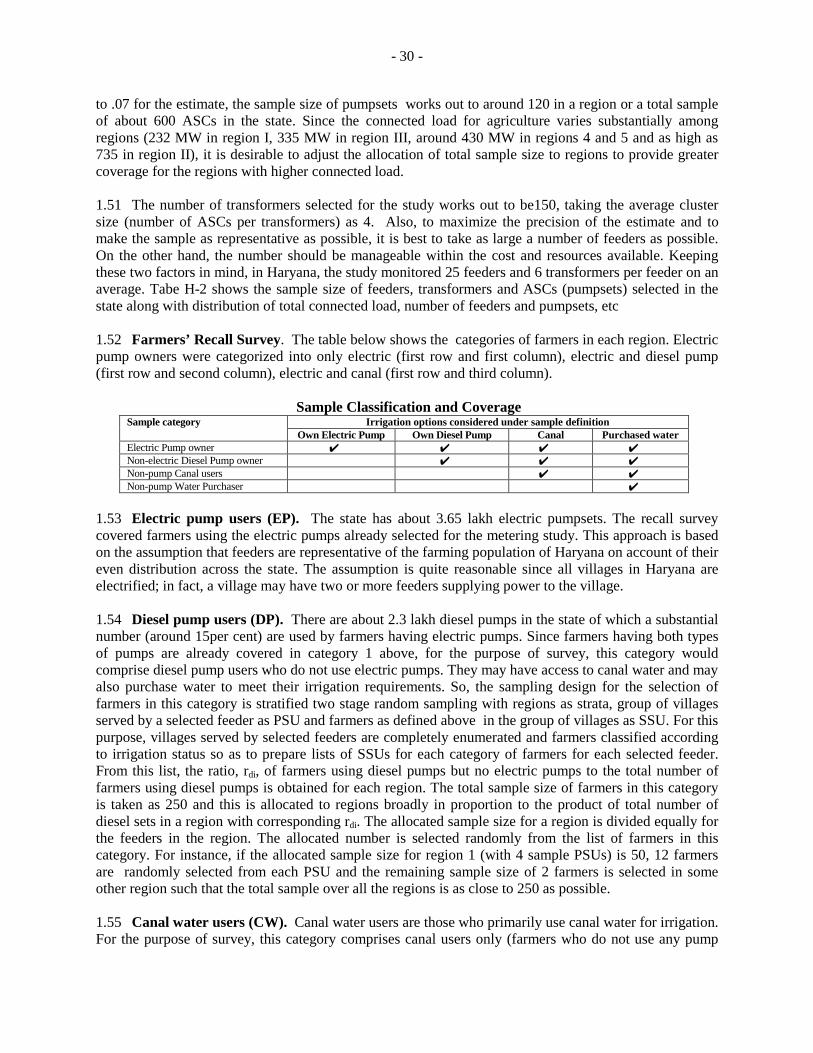
to .07 for the estimate, the sample size of pumpsets works out to around 120 in a region or a total sample of about 600 ASCs in the state. Since the connected load for agriculture varies substantially among regions (232 MW in region I, 335 MW in region III, around 430 MW in regions 4 and 5 and as high as 735 in region II), it is desirable to adjust the allocation of total sample size to regions to provide greater coverage for the regions with higher connected load. 1.51 The number of transformers selected for the study works out to be150, taking the average cluster size (number of ASCs per transformers) as 4. Also, to maximize the precision of the estimate and to make the sample as representative as possible, it is best to take as large a number of feeders as possible. On the other hand, the number should be manageable within the cost and resources available. Keeping these two factors in mind, in Haryana, the study monitored 25 feeders and 6 transformers per feeder on an average. Tabe H-2 shows the sample size of feeders, transformers and ASCs (pumpsets) selected in the state along with distribution of total connected load, number of feeders and pumpsets, etc 1.52 Farmers’ Recall Survey. The table below shows the categories of farmers in each region. Electric pump owners were categorized into only electric (first row and first column), electric and diesel pump (first row and second column), electric and canal (first row and third column).

Sample Classification and Coverage Irrigation options considered under sample definition Sample category

Own Electric Pump Own Diesel Pump Canal Purchased water Electric Pump owner ✔ ✔ ✔ ✔ Non-electric Diesel Pump owner ✔ ✔ ✔ Non-pump Canal users ✔ ✔ Non-pump Water Purchaser ✔

1.53 Electric pump users (EP). The state has about 3.65 lakh electric pumpsets. The recall survey covered farmers using the electric pumps already selected for the metering study. This approach is based on the assumption that feeders are representative of the farming population of Haryana on account of their even distribution across the state. The assumption is quite reasonable since all villages in Haryana are electrified; in fact, a village may have two or more feeders supplying power to the village. 1.54 Diesel pump users (DP). There are about 2.3 lakh diesel pumps in the state of which a substantial number (around 15per cent) are used by farmers having electric pumps. Since farmers having both types of pumps are already covered in category 1 above, for the purpose of survey, this category would comprise diesel pump users who do not use electric pumps. They may have access to canal water and may also purchase water to meet their irrigation requirements. So, the sampling design for the selection of farmers in this category is stratified two stage random sampling with regions as strata, group of villages served by a selected feeder as PSU and farmers as defined above in the group of villages as SSU. For this purpose, villages served by selected feeders are completely enumerated and farmers classified according to irrigation status so as to prepare lists of SSUs for each category of farmers for each selected feeder. From this list, the ratio, rdi, of farmers using diesel pumps but no electric pumps to the total number of farmers using diesel pumps is obtained for each region. The total sample size of farmers in this category is taken as 250 and this is allocated to regions broadly in proportion to the product of total number of diesel sets in a region with corresponding rdi. The allocated sample size for a region is divided equally for the feeders in the region. The allocated number is selected randomly from the list of farmers in this category. For instance, if the allocated sample size for region 1 (with 4 sample PSUs) is 50, 12 farmers are randomly selected from each PSU and the remaining sample size of 2 farmers is selected in some other region such that the total sample over all the regions is as close to 250 as possible. 1.55 Canal water users (CW). Canal water users are those who primarily use canal water for irrigation. For the purpose of survey, this category comprises canal users only (farmers who do not use any pump

- 31 -

although they may purchase water to meet their irrigation requirements). A list of canal water users only is prepared by complete enumeration of villages (as in 1.5 above). The sample size for canal users only is also 250. Since the total number of farmers in this category for a region is not available, the sample size of 250 is allocated to different regions broadly in proportion to the total number of farmers in this category as per listing based on complete enumeration of selected PSUs in a region. The allocated number for a region is then randomly selected after dividing it equally over the PSUs in that region as in 1.54 above. 1.56 Water purchasers (WP). Water purchasers are those who irrigate their land but do not have any source of irrigation (pump, canal) and their irrigation requirements are met from purchase of water from other farmers. Since charges for electricity used for running pumpsets are levied at flat rate and not on the basis of actual power use, sale/purchase of water is more likely in areas where use of electric pumps is prevalent. A list of water purchasers is prepared by complete enumeration of villages (as in 1.54 above). The sample size for this category of farmers is also 250 to be randomly selected after allocation to different regions as described in 1.55 above. 1.57 Farmers with unirrigated (rainfed) holdings (RF). Apart from farmers adopting one or the other irrigation technology option, some farmers do not have any access to water for irrigation and have to depend upon rain for growing crops. Farmers in this category have to decide upon the cropping pattern and input use in order to maximize the output under total irrigation constraint. Agricultural practices of these farmers will normally not be the same as those of farmers having a part of their land irrigated since farmers in the latter category are assured of output from irrigated land and therefore may not optimize the input use for the rainfed part of their holding. For the purpose of fitting of econometric model under partial equilibrium, some representation needs to be given to this category of farmers also. Accordingly, from the list of farmers with rainfed holdings available from complete enumeration of villages (as in 1.54 above), a sample of 150 farmers is randomly selected after allocation to different regions as described in 1.55 above. The sample description and sample size for various technology options are given in Appendix 2.1

- 32 -

Weighting Procedure for Haryana 1.58 After taking random samples from the mutually exclusive categories of farmers as above, we have to use appropriate weighting factors for aggregation of sample values to the region or the state level. For this purpose we need to have total population figures for each category as indicated in the table below.

Total Total SampleSamplePopulation Population Weight Feeder 1 ‘n’ of elec. ‘n’ of elec. N of elec. N of elec. Elec. pumps Elec. users pumps in F1 pumps in pumps in F1 pumps in represented by region region 1 sample case ‘n’ of diesel ‘n’ of diesel N of diesel N of diesel Diesel pumps Diesel users pumps in F1 pumps in pumps in F1 pumps in represented by region region 1 sample case ‘n’ of canal ‘n’ of canal N of canal N of canal Canal users Canal users users in F1 users in users in F1 users in represented by region region 1 sample case Water ‘n’ of water ‘n’ of water N of water N of water Water purchasers purchasers purchasers in purchasers purchasers in purchasers in F1 region in F1 region represented by 1 sample case Dry land ‘n’ of dry ‘n’ of dry N of dry N of dry Dry land farmers land farmers land farmers land farmers land farmers farmers in F1 in region in F1 in region represented by 1 sample case For canal users, water purchasers and dry land farmers, N of users in the region is not available. This is estimated by the proportion of users in the total number of farmers for the sampled feeders in a region. N of users of F1 (out of which ‘n’ will be sampled) for any category will be available by a complete enumeration of villages served by the selected feeders. 1.59 Tariff Cost Computation. The tariff cost for electric pump owners in this study was computed in the following way. Around 94% of electric pump owners in the sample reported paying on the basis of flat rate (ORG, Attitude Survey Report). For the calculation of the flat tariff amount per farmer, the district wise official tariff rate per HP was multiplied by the electric HP reported by the farmer11. This tariff cost imputation may differ from the actual amount paid by farmer because of several reasons:

• The HP reported by farmer in the survey might be different from the HP in utility records on the basis of which the tariff cost is actually assessed.

11 The district wise official tariff rate was calculated on the basis of groundwater depth recorded for maximum number of wells in each district. The information on groundwater depth was taken from the above-mentioned survey in 1998, which forms the basis of utility assessments of tariff rates.

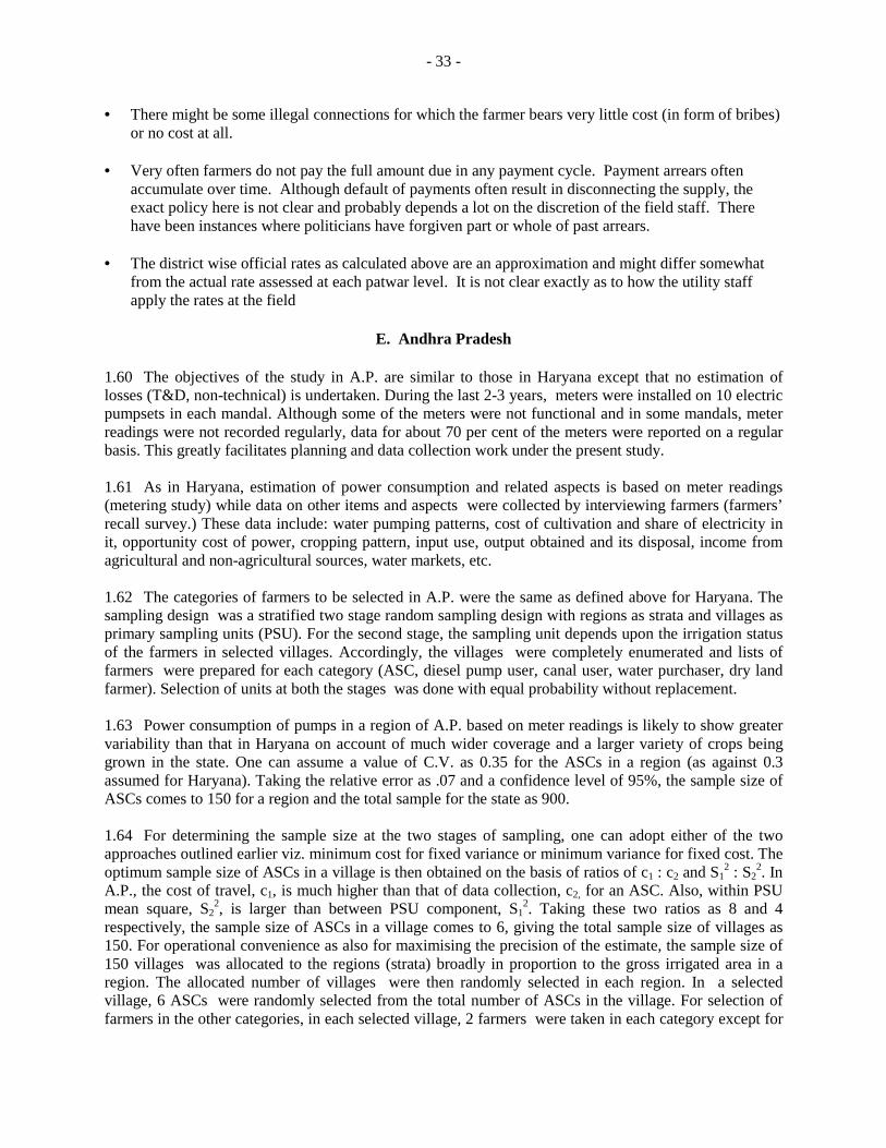
- 33 -

• There might be some illegal connections for which the farmer bears very little cost (in form of bribes) or no cost at all.

• Very often farmers do not pay the full amount due in any payment cycle. Payment arrears often

accumulate over time. Although default of payments often result in disconnecting the supply, the exact policy here is not clear and probably depends a lot on the discretion of the field staff. There have been instances where politicians have forgiven part or whole of past arrears.

• The district wise official rates as calculated above are an approximation and might differ somewhat

from the actual rate assessed at each patwar level. It is not clear exactly as to how the utility staff apply the rates at the field

E. Andhra Pradesh

1.60 The objectives of the study in A.P. are similar to those in Haryana except that no estimation of losses (T&D, non-technical) is undertaken. During the last 2-3 years, meters were installed on 10 electric pumpsets in each mandal. Although some of the meters were not functional and in some mandals, meter readings were not recorded regularly, data for about 70 per cent of the meters were reported on a regular basis. This greatly facilitates planning and data collection work under the present study. 1.61 As in Haryana, estimation of power consumption and related aspects is based on meter readings (metering study) while data on other items and aspects were collected by interviewing farmers (farmers’ recall survey.) These data include: water pumping patterns, cost of cultivation and share of electricity in it, opportunity cost of power, cropping pattern, input use, output obtained and its disposal, income from agricultural and non-agricultural sources, water markets, etc. 1.62 The categories of farmers to be selected in A.P. were the same as defined above for Haryana. The sampling design was a stratified two stage random sampling design with regions as strata and villages as primary sampling units (PSU). For the second stage, the sampling unit depends upon the irrigation status of the farmers in selected villages. Accordingly, the villages were completely enumerated and lists of farmers were prepared for each category (ASC, diesel pump user, canal user, water purchaser, dry land farmer). Selection of units at both the stages was done with equal probability without replacement. 1.63 Power consumption of pumps in a region of A.P. based on meter readings is likely to show greater variability than that in Haryana on account of much wider coverage and a larger variety of crops being grown in the state. One can assume a value of C.V. as 0.35 for the ASCs in a region (as against 0.3 assumed for Haryana). Taking the relative error as .07 and a confidence level of 95%, the sample size of ASCs comes to 150 for a region and the total sample for the state as 900. 1.64 For determining the sample size at the two stages of sampling, one can adopt either of the two approaches outlined earlier viz. minimum cost for fixed variance or minimum variance for fixed cost. The optimum sample size of ASCs in a village is then obtained on the basis of ratios of c1 : c2 and S1

2 : S22. In

A.P., the cost of travel, c1, is much higher than that of data collection, c2, for an ASC. Also, within PSU mean square, S2

2, is larger than between PSU component, S12. Taking these two ratios as 8 and 4

respectively, the sample size of ASCs in a village comes to 6, giving the total sample size of villages as 150. For operational convenience as also for maximising the precision of the estimate, the sample size of 150 villages was allocated to the regions (strata) broadly in proportion to the gross irrigated area in a region. The allocated number of villages were then randomly selected in each region. In a selected village, 6 ASCs were randomly selected from the total number of ASCs in the village. For selection of farmers in the other categories, in each selected village, 2 farmers were taken in each category except for

- 34 -

canal users for which the sample size is 3 farmers per village. The allocated number of villages and the number of ASCs/farmers in different regions are given in table A-2. The sample size may be slightly higher on account of joint use of selected electric pumps. The sample description and sample size for various technology options are given in Appendix 2.1 1.65 Metering Study. Meters were installed on all the ASCs selected as above and power consumption was estimated on the basis of meter readings taken at regular intervals. In case the number of ASC in a selected village was less than the number to be sampled, all the ASCs in the village were selected and the shortfall was made up by augmenting the sample in villages with larger number of ASCs. 1.66 Farmers’ Recall Survey. The selected ASCs as also farmers selected in the other categories were covered in the recall survey. Shortfall of sample size for any category of farmers in a selected village, if any, was made up by augmenting the sample size in other villages with larger number of farmers in that category. Data on various items and aspects were collected as in Haryana. Information similar to the table for Haryana is required for weighting of the samples to obtain average at the region and state level. 1.67 Estimation of mean and its variance. After collection of data (meter readings, farmers’ recall), the average/total of the parameter of interest and its variance/S.E. have to be estimated using appropriate statistical procedure. This obviously corresponds to the sampling design used for selection of PSUs/SSUs and the sample size of units at different sampling stages. While the estimation procedure for two stage random sampling is available in any standard text, the procedure for two stage cluster sampling (clustering being done at the second stage) is not readily available in the literature. The appropriate expressions for obtaining an unbiased estimate of mean and its variance for two stage cluster sampling has been developed. The corresponding expressions for the two design are given in Appendix 2.2. The terminology used and detailed estimation procedure for the estimates of mean and variance at the region and state levels for the two designs are given at the end of this section.

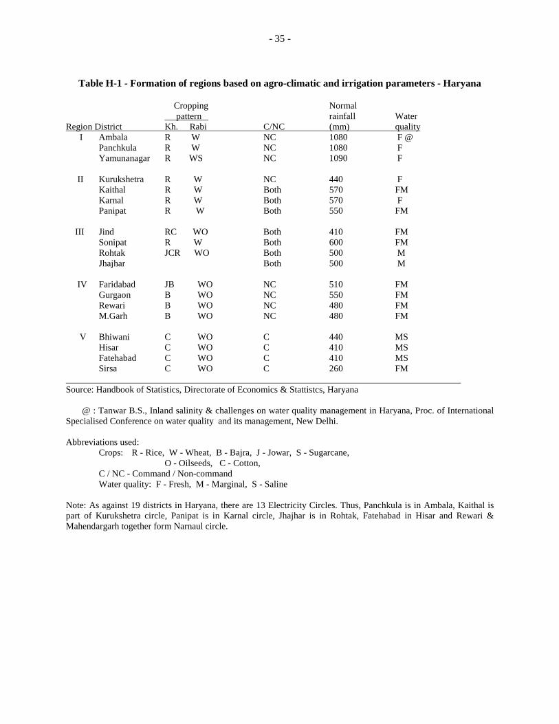
- 35 -

Table H-1 - Formation of regions based on agro-climatic and irrigation parameters - Haryana

Cropping Normal pattern rainfall Water Region District Kh. Rabi C/NC (mm) quality I Ambala R W NC 1080 F @ Panchkula R W NC 1080 F Yamunanagar R WS NC 1090 F II Kurukshetra R W NC 440 F Kaithal R W Both 570 FM Karnal R W Both 570 F Panipat R W Both 550 FM III Jind RC WO Both 410 FM Sonipat R W Both 600 FM Rohtak JCR WO Both 500 M Jhajhar Both 500 M IV Faridabad JB WO NC 510 FM Gurgaon B WO NC 550 FM Rewari B WO NC 480 FM M.Garh B WO NC 480 FM V Bhiwani C WO C 440 MS Hisar C WO C 410 MS Fatehabad C WO C 410 MS Sirsa C WO C 260 FM Source: Handbook of Statistics, Directorate of Economics & Stattistcs, Haryana @ : Tanwar B.S., Inland salinity & challenges on water quality management in Haryana, Proc. of International Specialised Conference on water quality and its management, New Delhi. Abbreviations used: Crops: R - Rice, W - Wheat, B - Bajra, J - Jowar, S - Sugarcane,

O - Oilseeds, C - Cotton, C / NC - Command / Non-command Water quality: F - Fresh, M - Marginal, S - Saline Note: As against 19 districts in Haryana, there are 13 Electricity Circles. Thus, Panchkula is in Ambala, Kaithal is part of Kurukshetra circle, Panipat is in Karnal circle, Jhajhar is in Rohtak, Fatehabad in Hisar and Rewari & Mahendargarh together form Narnaul circle.

- 36 -

Table H-2 - Connected load and sample size for metering and survey - Haryana Connected Number of load (MW) No. of Pumpsets No. of feeders No. of selected Region District Total Av. Villages Elec. Diesel$ Total Selected T/F Pumpsets I Ambala 232 0.97 1338 38352 16819 240 4 25 82 Panchkula (240) Yamunanagar II Kurukshetra 735 1.23 1273 143748 42112 593 7 35 219 Kaithal (593) Karnal Panipat III Jind 335 0.97 1022 42073 85591 344 4 21 113 Sonipat (344) Rohtak Jhajhar IV Faridabad 434 0.78 1870 91203 23055 556 5 25 114 Gurgaon (556) Rewari M.Garh V Bhiwani 422 0.87 1256 49667 58271 484 5 34 71 Hisar (484) Fatehabad Sirsa Total 2158 0.97 6759 365043 225848 2217 25 140 599 (2217) $ - Pertains to 1995 Note: 1. Figures in parentheses are the number of outgoing feeders.

2. The number of transformers and ASCs would be determined after selection of feeders. The total sample of ASCs in the state is proposed as 600.

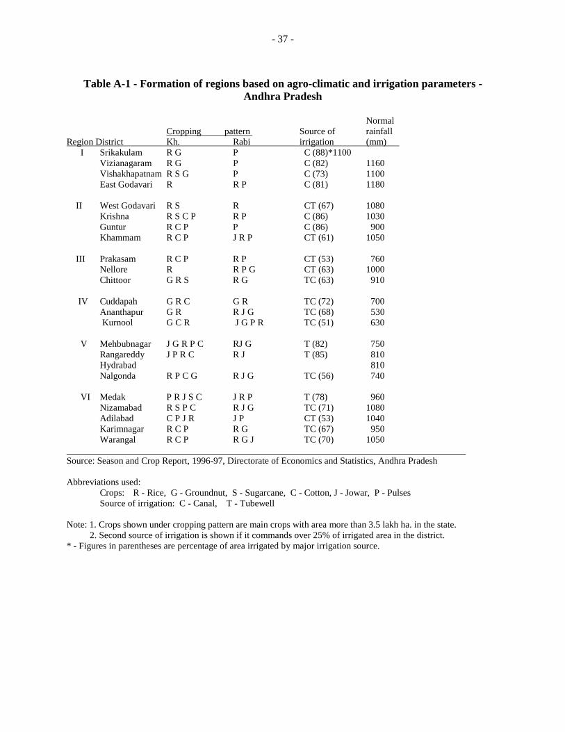
- 37 -

Table A-1 - Formation of regions based on agro-climatic and irrigation parameters -

Andhra Pradesh Normal Cropping pattern Source of rainfall Region District Kh. Rabi irrigation (mm) I Srikakulam R G P C (88)* 1100 Vizianagaram R G P C (82) 1160 Vishakhapatnam R S G P C (73) 1100 East Godavari R R P C (81) 1180 II West Godavari R S R CT (67) 1080 Krishna R S C P R P C (86) 1030 Guntur R C P P C (86) 900 Khammam R C P J R P CT (61) 1050 III Prakasam R C P R P CT (53) 760 Nellore R R P G CT (63) 1000 Chittoor G R S R G TC (63) 910 IV Cuddapah G R C G R TC (72) 700 Ananthapur G R R J G TC (68) 530 Kurnool G C R J G P R TC (51) 630 V Mehbubnagar J G R P C RJ G T (82) 750 Rangareddy J P R C R J T (85) 810 Hydrabad 810 Nalgonda R P C G R J G TC (56) 740 VI Medak P R J S C J R P T (78) 960 Nizamabad R S P C R J G TC (71) 1080 Adilabad C P J R J P CT (53) 1040 Karimnagar R C P R G TC (67) 950 Warangal R C P R G J TC (70) 1050 Source: Season and Crop Report, 1996-97, Directorate of Economics and Statistics, Andhra Pradesh Abbreviations used: Crops: R - Rice, G - Groundnut, S - Sugarcane, C - Cotton, J - Jowar, P - Pulses Source of irrigation: C - Canal, T - Tubewell Note: 1. Crops shown under cropping pattern are main crops with area more than 3.5 lakh ha. in the state. 2. Second source of irrigation is shown if it commands over 25% of irrigated area in the district. * - Figures in parentheses are percentage of area irrigated by major irrigation source.

- 38 -

Table A-2 - Connected load and sample size for metering and survey - Andhra Pradesh

Connected Number of Gross Sample size load (agri) No. of Pumpsets irrigated for survey Region District MW Mdl Vill. Elec. Diesel area(‘000ha) Vill. ASC Farmers* I Srikakulam 331.3 173 7593 79909 8766 988.9 23 138 207 Vizianagaram Vishakhapatnam East Godavari II West Godavari 713.4 199 3573 164261 14289 1633.4 35 210 315 Krishna Guntur Khammam III Prakasam 1000.6 168 3579 300549 24254 782.6 22 132 198 Nellore Chittoor IV Cuddapah 869.1 167 2704 208773 9683 567.9 20 120 180 Ananthapur Kurnool V Mehbubnagar 1274.8 164 3472 356687 25762 595.2 20 120 180 Rangareddy Hydrabad Nalgonda VI Medak 1809.6 239 5692 681044 18887 1214.3 30 180 270 Nizamabad Adilabad Karimnagar Warangal Total 5998.8 1100 26613 1791203 101641 5782.2 150 900 1350 * - In each village, 6 ASCs and 9 other farmers (3 surface water users and 2 each of diesel pump users, water purchasers and dry land farmers) to be randomly selected from lists prepared by complete enumeration of the selected villages.

- 39 -

Appendix II.1

Irrigation Technology Options, Sample Description and Sample Size Sample size S.No. Irrigation Technology Option Sample Description Haryana A.P. 1. Electric pump only (EP) | Electric pump users 600 900 2. Electric and diesel pumps (EDP) | with or without diesel pump, 3. Electric pump and surface water | surface water, purchased water 4. Electric and diesel pumps and | surface water 5. Diesel pump only | Diesel pump users 250 300 6. Diesel pump and surface water | with or without surface water, purchased water 7. Surface water only Surface water users 250 450 (without any pump) without any pump, with or without purchased water 8. Water purchasers Farmers irrigating land with 250 300 no source of irrigation 9. Dry land farmers Farmers with entire holding 150 300 (unirrigated holdings) uniirigated Total Sample 1500 2250

- 40 -

Appendix II.2

Procedure For Estimation of Mean and Estimate of its Variance 1. Stratified two-stage cluster sampling design In Haryana, the design adopted for estimation of power consumption in agriculture is stratified two stage cluster sampling. The state has been divided into 5 agro-climatic regions, which constitute the strata. Agricultural feeders in a region are the primary sampling units (PSU) and transformers on a feeder are the second stage units (SSU). All the pumpsets (P/S) receiving power from a selected transformer will be taken for the study. Since the number of pumps varies from one transformer to another and, similarly, the number of transformers varies over feeders, the sampling units at both the stages of sampling are of unequal size. Estimates of parameters of interest may be obtained at the region level and these may then be aggregated using appropriate weights to obtain estimate at the state level. The procedure for estimation of mean power consumption per pump of a pumpset and the estimate of its variance is described below. A similar procedure is adopted for estimation of other parameters of interest. For a given region (stratum), let N denote the number of agricultural feeders and Mi the number of transformers on the ith feeder with corresponding sample values being denoted by n and mi. Let Lij denote the number of pumpsets receiving power from the jth transformer on the ith feeder (i=1, ..n, j=1, ..mi for the sample and i=1, ..N, j=1, ..Mi and k=1, ..Lij for the population). The total number of SSUs in the population, M0, is given by N M0 = N M where M = 1/N(Σ Μi) . ι=1

Let yijk denote the power consumption per pump of the kth pumpset of the (i,j) th transformer. The average power consumption per pump of the (i,j)th transformer is given by Lij yij = 1/ Lij ( Σ yijk ) κ=1

Then the average consumption per pump for the ith feeder is given by mi yi = 1/mi Σ (Lij/ Li ) yij , j=1 where Li is the average number of pumpsets per transformer of the ith feeder and is given by Mi

Li = Li0 / Mi where Li0 = Σ Lij j=1

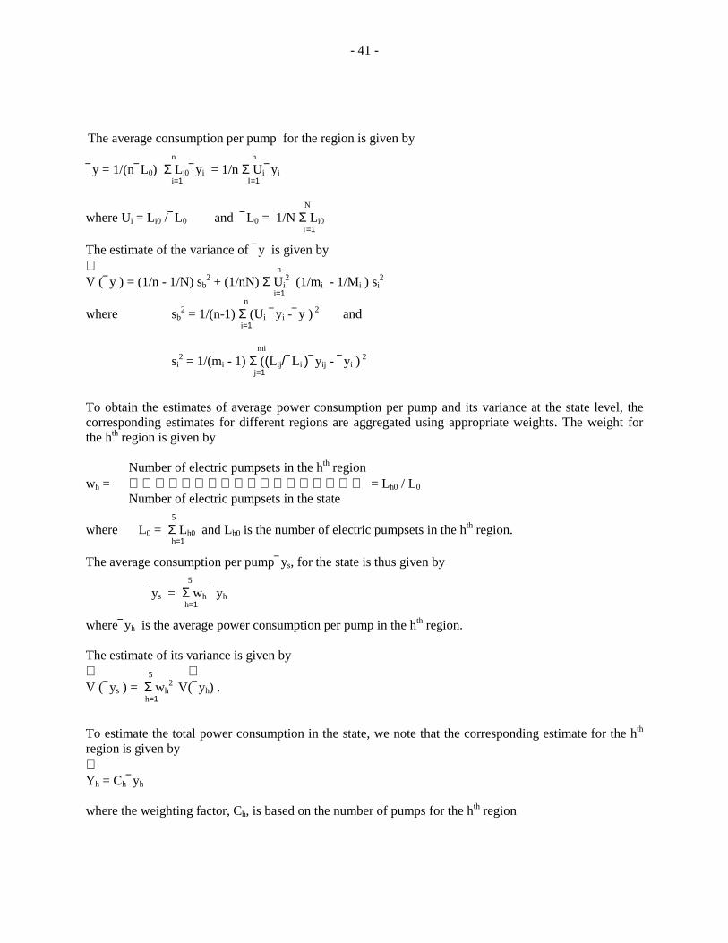
- 41 -

The average consumption per pump for the region is given by n n y = 1/(n L0) Σ Li0 yi = 1/n Σ Ui yi i=1 Ι=1

N

where Ui = Li0 / L0 and L0 = 1/N Σ Li0 ι=1 The estimate of the variance of y is given by ∧ n V ( y ) = (1/n - 1/N) sb

2 + (1/nN) Σ Ui2 (1/mi - 1/Mi ) si

2

n i=1 where sb

2 = 1/(n-1) Σ (Ui yi - y ) 2 and i=1

mi si

2 = 1/(mi - 1) Σ ((Lij/ Li ) yij - yi ) 2 j=1 To obtain the estimates of average power consumption per pump and its variance at the state level, the corresponding estimates for different regions are aggregated using appropriate weights. The weight for the hth region is given by Number of electric pumpsets in the hth region wh = = Lh0 / L0 Number of electric pumpsets in the state 5 where L0 = Σ Lh0 and Lh0 is the number of electric pumpsets in the hth region. h=1 The average consumption per pump ys, for the state is thus given by 5 ys = Σ wh yh h=1 where yh is the average power consumption per pump in the hth region. The estimate of its variance is given by ∧ 5 ∧ V ( ys ) = Σ wh

2 V( yh) . h=1 To estimate the total power consumption in the state, we note that the corresponding estimate for the hth region is given by ∧ Yh = Ch yh where the weighting factor, Ch, is based on the number of pumps for the hth region

- 42 -

The estimate of its variance is given by ∧ ∧ ∧ V (Yh ) = Ch

2 V ( yh ). ∧ The aggregates of Yh and the estimate of its variance over the regions provide the corresponding estimates at the state level. Although the total number of electric pumpsets in a region Lh0 is available for each region, the total number of farmers (SSUs) for some of the other categories like canal users, water purchasers, etc. may not be available for each region. In this case, the total number of SSUs in a category is estimated on the basis of its proportion in the selected PSUs in a region as follows: ∧ n n Lh0 = ∑ Lhi / ∑ Fhi h=1 h=1 where Lhi is the total number of SSUs belonging to a specific category in the ith PSU of the hth region and Fhi is the correspondingly the total number of farmers in the ith PSU of the hth region. To obtain the estimates of the mean and variance of the character under study for the state, the weighting factor for the hth region is given by ∧ n ∧ wh = Lh0 / Σ Lh0 . h=1

- 43 -

2. Stratified two-stage random sampling design As in Haryana, the state of Andhra Pradesh has been divided into 6 regions which constitute the strata. In a region, villages are the primary sampling units (PSU) and ASCs/ farmers are the second stage units (SSU). For a region let N denote the number of villages (PSUs) and Mi the number of ASCs/farmers (SSUs) in the ith village with n and mi denoting the corresponding sample values. (i=1, ..N, j=1, ..Mi for the population and i=1, ..n, j=1, ..mi for the sample). Let yij denote the power consumption per HP for the jth pumpset in the ith village. Then y, the estimate of average power consumption per HP is given by n mi N y = 1/(n M) Σ Mi yi where yi = 1/ mi Σ yij and M = 1/N Σ Mi i=1 j=1 i=1

n = 1/n Σ Ui yi where Ui = Mi / M i=1 The estimate of the variance of y is given by ∧ n V ( y ) = (1/n - 1/N) sb

2 + (1/nN) Σ Ui2 (1/mi - 1/Mi ) si

2

n i=1 where sb

2 = 1/(n-1) Σ (Ui yi - y ) 2 and i=1

mi si

2 = 1/(mi - 1) Σ ( yij - yi ) 2 j=1 In the above procedure, it is assumed that Mi, the total number of pumpsets in a village, is available for all the villages (PSUs) in a region. If this is not the case, we may use M′ in place of M where M′ is given by n M′ = 1/n Σ Mi . i=1 To obtain the estimates of average power consumption per HP and its variance at the state level, the corresponding estimates for different regions will be aggregated using appropriate weights as described above. The estimates of the total power consumption and its variance at the state level may also be obtained by following the corresponding procedure described above.