Indexing the Present and Future Positions of Moving Objects Simonas Šaltenis Aalborg University Nykredit Center for Database Research Department of Computer

Indexing the Present and Future Positions of Moving Objects

Simonas ŠaltenisAalborg University

Nykredit Center for Database ResearchDepartment of Computer Science, Aalborg University

LBS workshop, Aalborg, June 7-8, 2001 2

Motivation – Background

• Position-aware, online, moving objects are enabled by the following trends.

Miniaturization of electronics Advances in positioning systems (e.g., GPS, assisted GPS, ...) Advances in wireless communications

• Examples of position-aware online moving objects WAP-enabled mobile-phones, as well as diverse types of personal

digital assistants (online “cameras,” “wrist watches,” etc.) By 2005, there wil be 500 million users of mobile phones with GPS.

Vehicles, including cars, public transportation, recreational vehicles, sea vessels, etc.

The coming years will witness very large quantities of these.


Motivation – Sample E-Services

• Traffic coordination and management Identification of impending traffic jams and expected fastest routes

between positions

• Location-aware advertising Consumers may receive sales information for locations close to

them. Here, the positional data is used together with an accumulated user profile to provide a better service.

• Integrated tourist services For example, this covers booking (hotels, concerts, ferries, etc.) and

payment, and provision of transportation or travel directions.

• Safety-related services It is possible to monitor tourists traveling in dangerous

environments, and then react to emergencies.


Motivation – Problem Statement

We address the problem of indexing the ever-changing current and predicted future positions of point objects moving in one, two, and three-dimensional space.

This also includes continuous variables in process monitoring, e.g., temperature, pressure (1D, nD).


Outline

• Data and queries• The TPR-tree

Bounding rectangles and insertion The inner workings of the tree Performance experiments

• Nothing is eternal... ...neither is positional information

• Conclusions


Spatial Indexing With the R-Tree

• The R-tree supports updates, but not continuous movement.

• Example

QueryR1

R2

R1 R2

R3 R4 R5

p6 p7p5p1 p2

Pointers to data tuples

p8

p3 p4 p9 p10p11 p12p13

R6 R7

R3 R4

R5

R6

R7

p1

p7

p6

p8

p2

p3

p4

p5

p9 p10

p11

p12

p13


Modeling Continuous Movement

• In conventional databases, data is assumed constant unless explicitly modified.

• With continuous movement, this is problematic. Too frequent updates Outdated, inacurate data



• In conventional databases, data is assumed constant unless explicitly modified.

• With continuous movement, this is problematic. Too frequent updates Outdated, inacurate data

• Instead of storing position values, we store positions as functions of time, yielding time-parameterized positions.

We use linear functions to capture the present and future positions.

Updates are necessary only when the parameters of the functions change. For example, given , the current and anticiapted, future position of a two-

dimensional point can be described by four parameters.

where,)()()( 00 nowtttvtxtx

0t

yx vvtytx ,),(),( 00



• Three ways to think about continuously moving points in d-dimensional space:

Lines in (d+1)-dimensional space d spatial dimensions and 1 time dimension

Points in 2d-dimensional space d spatial and d velocity dimensions (function parameters: )

Time-parameterized points in d-dimensional space – our approach

vtx ),( 0

x

t2 3 4 5 6

1o1

23456

1

o2

o3

v0 0.5 1

1

23456

x(t0)

-0.5

o1

o2

o3


Queries

• Type 1: objects that intersect a given rectangle at

• Type 2: objects that intersect a given rectangle sometime from to

• Type 3: objects that intersect a given moving rectangle sometime between and

1t 2t

1t 2t

t

1

23456x

t1 2 3 4 5 6

o1

o1o2

o3

o4


Time-Parameterized Rectangles

• The TPR-tree is based on the R-tree.

• Moving points are bounded with time-parameterized rectangles.

Are bounding from now on. The R-tree allows overlap.

• Ideally, bounding rectangles should be always minimal.

Excessive storage cost

• The tree employs conservative bounding rectangles.

• These are ”tightened” during modifications.

nodeovov

nodeovov

nodeotxotx

nodeotxotx

ii

ii

cici

cici

.max

.min

)(.max)(

)(.min)(

max

min

max

min


Insertion: Grouping Points

• How to group moving points? The R-tree’s algorithms minimize characteristics of MBRs such as

area, overlap, and margin. How does that work for moving points?

7

1

6

5

4

2

3

7

5

6

4

2

31

6

5

4

2

31

7

7

5

6

4

2

31

7

5

6

4

2

31

7

5

6

4

2

31


Insertion in the TPR-Tree

• The bounding rectangle characteristics (area, overlap, and margin) are functions of time.

• The goal is to minimize these for all time points from now to now+H.

Minimizing the characteristics for time now + H/2 does not work (e.g., the area of a conservative bounding rectangle is not linear).

,Hnow

now

dttA )( where A(t) is, e.g., the area of an MBR

• We use the regular R*-tree algorithms, but all bounding rectangle characteristics are replaced by their integrals.

• What H to use? H depends on the update rate, and on how far queries may reach

into the future (W).


Example I

• We illustrate the working of the TPR-tree by means of an example.

The subsequent figures are generated automatically, by the index code used for performance experiments.

• Data 20 one-dimensional points are used.

• Index Parameters Page size = 64 (5 entries in leaf nodes and 3 in non-leaf nodes). H = 8.


Example II

CT = 0

At CT=1, the point at x = 20, v = 0 is updated to have x = 18.5, v = -0.5.


Example III

CT = 1

Inserting a moving point at position 14 with v = –0.5.


Example IV

After insertion


Performance Experiments I

• Simulation-based performance study A GIST-based implementation of the TPR-tree is used.

• Trees are initially bulk loaded, then subjected to workloads intermixing modifications and queries for 600 minutes.

1000 x 1000 km space and from 100,000 to 900,000 point objects. The speeds of the objects range from 0 to 180 km/h. On average, each object sends an update each 60 minutes

(yielding a total of from 1,666 to 15,000 updates per minute). 2D and 3D uniform data is used, as well as 2D data generated

according to a scenario, where objects move on a fully connected graph of two-way roads.

• Indices compared Straigthforward R-tree TPR-tree TPR-tree with load-time bounding rectangles


Performance Experiments III

• Search performance for 2D data with varying skew (the number of destinations).

• The more objects move similarly, the easier it is to index them.

• Tightening of bounding rectangles on updates results in a significant decrease in the search I/O.

Not possible with the dual transformation.


Performance Experiments IV

• Degradation of search performance across time for 2D data, with W = 40.

• Due to the constant influx of updates, the performance of the TPR-tree does not degrade after reaching a certain level.


Performance Experiments V

• Search performance for 2D data with varying numbers of moving objects (average # of returned objects per query is not changed).

• As expected, the TPR-tree shows almost no decrease in performance (as long as the number of tree levels does not change).


Improving the TPR-tree• Coping with out-dated data

In the highly dynamic environment of moving objects data becomes inaccurate and obsolete very fast.

Unreliable communication channels lead to no guaranties of objects updating or deleting themselves.

• Solution – expiration time texp associated with each object Expiration times depend on (or can be derived from):

Desired uncertainty threshold and speeds of objects Underlying infrastructure (e.g., road network) restricting movement

• Expiration times may be a good idea even if objects always update and delete themselves on time.

Indexing segments of future trajectories instead of infinite lines should be easier .


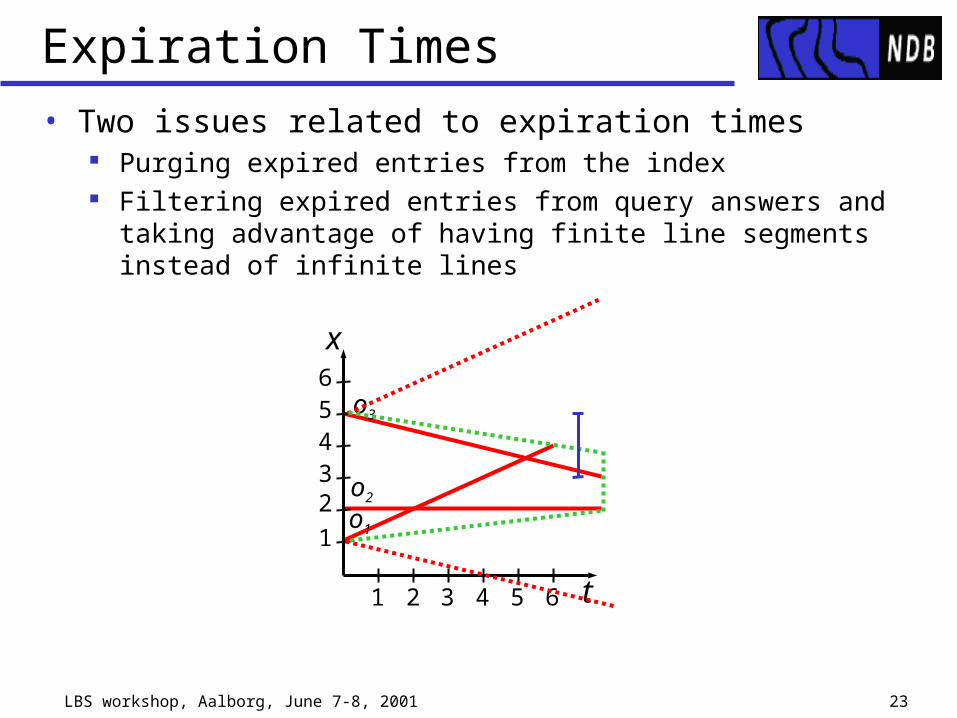
Expiration Times

• Two issues related to expiration times Purging expired entries from the index Filtering expired entries from query answers and taking advantage

of having finite line segments instead of infinite lines

x

t2 3 4 5 6

1o1

23456

1

o2

o3


Purging Expired Entries I

• Purging done in a lazy fashion – expired entries are ignored in all index algorithms and they are physically removed when a node is written to the disk.

• Insertion and deletion algorithms are modified to account for under-full nodes at any stage of the algorithm.


Purging Expired Entries II


Conclusions

• The TPR-tree indexes the current and predicted future positions of moving objects.

The TPR-tree is based on the proven, widely used R-tree technology

The tree extends the R*-tree by introducing conservative, time-parameterized bounding rectangles, which are tightened regularly.

The tree’s algorithms use integrals of area, overlap, etc. The tree can be tuned to take advantage of a specific update rate

and querying window length. Out-dated data can be automatically purged from the index Other types of queries that are supported by the R-tree can be

supported by the TPR-tree, e.g., nearest-neighbor queries.

Documents

Indexing the Present and Future Positions of Moving Objects Simonas Šaltenis Aalborg University Nykredit Center for Database Research Department of Computer