CS6200 Information Retrieval Indexing

Indexing

June 12, 2015

1 Documents and query representation

Documents can be represented in the form of an Incidence matrix of a graph which gives (0,1) matrix havinga row for each vertex and column for each edge, and (v,e) is 1 iff vertex v is incident upon edge e. - Skiena1990, pg 135

(a) Graph(b) Incidence Matric

Figure 1: A graph and its Corresponding Incidence Matric

1.1 Bag of words

· Term Frequency : we assign to each term in a document a weight for that term, that depends on thenumber of occurrences of the term in the document. We would like to compute a score between a queryterm t and a document d, based on the weight of t in d. The simplest approach is to assign the weightto be equal to the number of occurrences of term t in document d. This weighting scheme is referredto as term frequency and is denoted tf t,d, with the subscripts denoting the term and the document inorder.

· Document Frequency : Document Frequency is defined to be the number of documents in the collectionthat contain a term t.

· Document Length : The Number of terms contained in a document indicate the length of the document.There are other ways to calculate the document length where document is represented in the form of

a xV ector−−−−→ x1, x2, x3, ..., xn is a vector in an n-dimensional vector space and length is denoted as

n√x21 + x22 + x23 + ...+ x2n

· Vocabulary : Denotes the Vocabulary size and indicates the number of unique terms in the document.

· N : Total number of documents in a collection is denoted by N

1

· Inverse Document Frequency : inverse document frequency of a term t as follows:

idft = logN

dft.

The idf of a rare term is high, whereas the IDF of a frequent term is likely to be low.

1.2 Retrieval Models

1.2.1 Okapi TF

This is a vector space model using a slightly modified version of TF to score documents. The Okapi TFscore for term w in document d is as follows.

okapi tf(w, d) =tfw,d

tfw,d + 0.5 + 1.5 · (len(d)/avg(len(d)))

Where:

• tfw,d is the term frequency of term w in document d

• len(d) is the length of document d

• avg(len(d)) is the average document length for the entire corpus

The matching score for document d and query q is as follows.

tf(d, q) =∑w∈q

okapi tf(w, d)

1.2.2 TF-IDF

This is the second vector space model. The scoring function is as follows.

tfidf(d, q) =∑w∈q

okapi tf(w, d) · logD

dfw

Where:

• D is the total number of documents in the corpus

• dfw is the number of documents which contain term w

1.2.3 Okapi BM25

BM25 is a language model based on a binary independence model. Its matching score is as follows.

bm25(d, q) =∑w∈q

log

(D + 0.5

dfw + 0.5

)· tfw,d + k1 · tfw,d

tfw,d + k1

((1− b) + b · len(d)

avg(len(d))

) · tfw,q + k2 · tfw,q

tfw,q + k2

Where:

• tfw,q is the term frequency of term w in query q

• k1, k2, and b are constants. You can use the values from the slides, or try your own.

2

1.2.4 Unigram LM with Laplace smoothing

This is a language model with Laplace (“add-one”) smoothing. We will use maximum likelihood estimatesof the query based on a multinomial model “trained” on the document. The matching score is as follows.

lm laplace(d, q) =∑w∈q

log p laplace(w|d)

p laplace(w|d) =tfw,d + 1

len(d) + V

Where:V is the vocabulary size – the total number of unique terms in the collection.

1.2.5 Unigram LM with Jelinek-Mercer smoothing

This is a similar language model, except that here we smooth a foreground document language model witha background model from the entire corpus.

lm jm(d, q) =∑w∈q

log p jm(w|d)

p jm(w|d) = λtfw,d

len(d)+ (1− λ)

∑d′ tfw,d′∑d′ len(d′)

Where:λ ∈ (0, 1) is a smoothing parameter which specifies the mixture of the foreground and background

distributions.

2 Preprocessing

In Information Retrieval, it is often necessary to interpret natural text where a large amount of text has tobe interpreted, so that it is available as a full text search and is represented efficiently in terms of both space(document storing) and time (retrieval processes) requirements.

It can also be regarded as : process of incorporating a new document into an information retrieval sys-tem. The document would go through the phases of Tokenization where the documents is broken downinto tokens, after which stopwords would be removed, thereafter stemming of the tokens takes place : whichstems each word into its root words and finally its all combined with term position to make an Index. We’llsee each of the processes as follows.

2.1 Tokenization

Tokenization is the task of chopping it up into pieces, called tokens, perhaps at the same time throwing awaycertain characters, such as punctuation. Input: ”John DavenPort #person 52 years old #age”

John DavenPort person 52 years old age

2.2 Stopwords

Stopwords refer to the words that have no meaning for ”Retrieval Purposes”. E.g.

· Articles : a, an, the, etc.

· Prepositions : in, on, of, etc.

· Conjunctions : and, or, but, if, etc

· Pronouns : I, you, them, it, etc

· Others : some verbs, nouns, adverbs, adjectives (make, thing, similar, etc.).

3

Stopwords can be up to 50% of the page content and not contribute to any relevant information w.r.t.retrieval process. Removal of these can improve the size of the index considerably. Sometimes we need tobe careful in terms of words in phrases! e.g.: Library of Congress, Smoky the Bear!

Word Occurrences Percentagethe 8,543,794 6.8of 3,893,790 3.1to 3,364,653 2.7

and 3,320,687 2.6in 2,311,785 1.8is 1,559,147 1.2for 1,313,561 1.0

that 1,066,503 0.8said 1,027,713 0.8

2.3 Stemming

Stemming is commonly used in Information Retrieval to conflate morphological variants. Typical stemmerconsists of collection of rules and/or dictionaries. Similar approach may be used in other languages too!

e.g.: The following stem to the word as shown below:servomanipulator ←− servomanipulators servomanipulatorlogic ←− logical logic logically logics logicals logicial logiciallylogin ←− login loginsmicrowire ←− microwires microwireknead ←− kneaded kneads knead kneader kneading kneaders

2.3.1 Stemming Example

Original text Porter StemmerDocument will describe marketing strategiescarried out by U.S. companies for their agri-cultural chemicals, report predictions for mar-ket share of such chemicals, or report mar-ket statistics for agrochemicals, pesticide, her-bicide, fungicide, insecticide, fertilizer, pre-dicted sales, market share, stimulate demand,price cut, volume of sales

market strateg carr compan agricultur chemicreport predict market share chemic reportmarket statist agrochem pesticid herbicidfungicid insecticid fertil predict sale stimul de-mand price cut volum sale

2.3.2 Porter Stemmer

There are multiple approaches for Stemming like using Brute force look up, Suffix - affix stripping, Part-of-speech recognition, Statistical algorithms (n-grams, HMM), etc.

Steps involved in Porter Stemmer:

1. Gets rid of plurals and -ed or -ing suffixes. e.g: Operatives → operative

2. Turns terminal y to i when there is another vowel in the stem. e.g: Coolly → coolli

3. Maps double suffixes to single ones: -ization, -ational, etc. e.g: Operational → operate

4. Deals with suffixes, -full, -ness etc.e.g: Authenticate → authentic

5. Takes off -ant, -ence, etc. e.g: Operational → operate → oper

6. Removes a final -e. e.g: Parable → parabl

4

2.3.3 Porter Stemming Example

· Step 1 : Semantically → semantically

· Step 2 : Semantically → semantically → semanticalli

· Step 3 : Semantically → semantically → semanticalli → semantical

· Step 4 : Semantically → semantically → semanticalli → semantical → semantic

· Step 5 : Semantically → semantically → semanticalli → semantical → semantic → semant

· Step 6 : Semantically → semantically → semanticalli → semantical → semantic → semant → semant

2.4 Term Positions

Term Positions specify the document id along with the position of occurrences in that specific document.Lets try and see that with an example. We have three documents of id1, id2 and id3:

id1 → 1Web

2Mining

3is

4useful

id2 → 1usage

2mining

3applications

id3 → 1Web

2structure

3mining

4studies

5the

6web

7hyperlink

8structure

The below figure summarizes the term positions:

3 Index Construction

A reasonably-sized index of the web contains many billions of documents and has a massive vocabulary.Search engines run roughly 105 queries per second over that collection. We need fine-tuned data structuresand algorithms to provide search results in much less than a second per query. O(n) and even O(log n)algorithms are often not nearly fast enough. The solution to this challenge is to run an inverted index on amassive distributed system.

Text search has unique needs compared to, e.g., database queries, and needs its own data structures’primarily, the inverted index and we’ll be discussing primarily the inverted index.

· Forward Index : A forward index is a map from documents to terms (and positions). These are usedwhen you search within a document.

· Inverted Index : An inverted index is a map from terms to documents (and positions). These are usedwhen you want to find a term in any document.

5

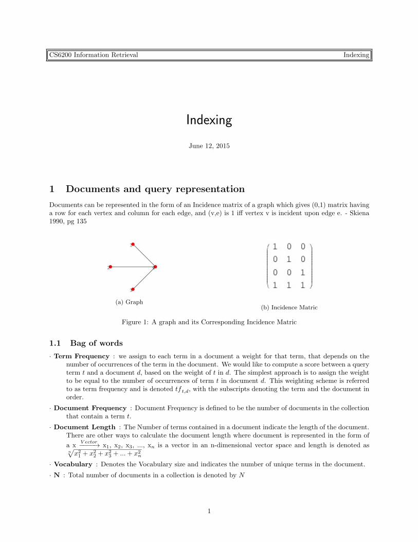
3.1 Inverted lists and catalog/offset files

In an inverted index, each term has an associated inverted list. At minimum,this list contains a list of identifiers for documents which contain that term.Usually we have more detailed information for each document as it relatesto that term. Each entry in an inverted list is called a posting. Documentpostings can store any information needed for efficient ranking. For instance,they typically store term counts for each document - tf w,d .

Depending on the underlying storage system, it can be expensive to increasethe size of a posting. It’s important to be able to efficiently scan through aninverted list, and it helps if they’re small.

Inverted Indexes are primarily used to allow fast, concurrent query pro-cessing. Each term found in any indexed document receives an independentinverted list, which stores the information necessary to process that term whenit occurs in a query. Next, we’ll see how to process proximity queries, whichinvolve multiple inverted lists.

3.2 Memory Structure, and limitations

Given a collection of documents, how can we efficiently create an inverted index of its contents? The basicsteps are:

1. Tokenize each document, to convert it to a sequence of terms.

2. Add doc to inverted list for each token.

This is simple at small scale and in memory, but grows much more complex to do efficiently as thedocument collection and vocabulary grow.

The basic indexing algorithm will fail as soon as you run out of memory. To address this, we store apartial inverted list to disk when it grows too large to handle. We reset the in-memory index and start over.When we’re finished, we merge all the partial indexes. The partial indexes should be written in a mannerthat facilitates later merging. For instance, store the terms in some reasonable sorted order. This permitsmerging with a single linear pass through all partial lists.

There are multiple ways as given below by which a Inverted Index can be built.

3.2.1 Option 1: Multiple Passes

Making multiple passes through the document collection is the key here. In each pass, we create the invertedlists for the next 1,000 terms, each in its own file. At the end of each pass, we concatenate the new invertedlists onto the main index file. This process is easy to concatenate the inverted files, but have to manage thecatalog/offsets files.

3.2.2 Option 2: Partial inverted lists

Create partial inverted lists for all terms in a single pass through the collection is what happens in thisprocess. As each partial list is filled, append it to the end of a single large index file. When all documentshave been processed, run through the file a term at a time and merge the partial lists for each term. Thissecond step can be greatly accelerated if you keep a list of the positions of all the partial lists for each termin some secondary data structure or file.

3.2.3 Option 3: preallocate the right amount of space

We could have dis-contiguous postings also. Here, we lay our index file as a series of fixed-length records of,say, 4096 bytes each. Each record will contain a portion of the inverted list for a term. A record will consistof a header followed by a series of inverted list entries. The header will specify the term id, the numberof inverted list entries used in the record, and the file offset of the next record for the term. Records are

6

written to the file in a single pass through the document collection, and the records for a given term are notnecessarily adjacent within the index.

3.3 Merging

Merging addresses limited memory problem. The main steps is shown as following:

1. Build the inverted list structure until memory runs out.

2. Then write the partial index to disk, start making a new one.

3. At the end of this process, the disk is filled with many partial indexes, which are merged.

There are two main partial index methods: by documents and by terms.

3.3.1 Merging partial-by-docs inverted indexes

1. parse and build temp file: for each document, parse text into terms assign a term to a termID(useinternal index for this). And for each distinct term in the document, write an entry to a temporaryfile with only triples (termID, docID, tf).

2. make sorted runs, to prepare for merging: sort the triples in memory by termID and docID,write them out into a sorted run on disk. See Figure 2

3. merge the runs: merge the sorted runs into a single run. See Figure 3

4. for each district term in final sorted run: start a new inverted file entry, read all triples for a giventerm, and build the posting list(feel free to use compression). Then write(append) this entry to theinverted index into file. See Figure 4

7

Figure 2: Sorted Runs

8

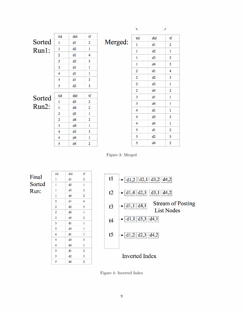
Figure 3: Merged

Figure 4: Inverted Index

9

3.3.2 Merging partial-by-terms inverted indexes

Merging partial index by terms is easier than merging by documents, but it may take longer time. The basicidea of partial-by-terms is that: for each term or part of terms, scan all documents and build its or theirinverted index until all the terms are processed.

3.4 Updating an inverted index

If each term’s inverted list is stored in a separate file, updating the index is straightforward: we simply mergethe postings from the old and new index. However, most filesystems can’t handle very large numbers of files,so several inverted lists are generally stored together in larger files. This complicates merging, especially ifthe index is still being used for query processing. There are ways to update live indexes efficiently, but it’soften simpler to simply write a new index, then redirect queries to the new index and delete the old one.

4 Proximity Search

Proximity is the search technique used to find two words next to, near, or within a specified distance of each

other within a document. Using such search operators may result in more satisfactory results that are more

relevant to the research needs than by just typing in desired keywords. Some commands also control the

terms’ order of appearance. Desired words can be in any order, a specific order, or within a certain range of

each other. The score function is based on the min span

λs−kk

where λ is a constant base, around 0.8, s is the min span found and k is the length ofngram matched.

e.g.: If ngram = ”atomic bomb world war two” matches on a min span of 8 words, thescore will be

λ8−55 = 0.80.6

Refer http://stevekrenzel.com/articles/blurbs for minimum span algorithm.

5 Other things to store in the index

Things which you can store in an index other than just postings list:

· Meta Information : Various other meta information such as summary term information,summary document information, etc. can be kept in the index which can be furtherused for efficient retrieval in meta data queries.

· Document Meta-data : The following information can be kept in the index too viz.language, geographic region, file format, date published, domain, licensing rights, etc.

· TimeStamp : Last updated timestamp or last crawled timestamp.

· Header Information : Like the number in the header of a posting list can indicate thenumber of posting units it contains and so on.

A: index storage organization (header) skives 1 : add lempel zif

10

6 Compression

Compressing indexes is important to conserve disk and/or RAM space. Inverted lists haveto be decompressed to read them, but there are fast, lossless compression algorithms withgood compression ratios.

6.1 Restricted Variable-Length Codes

An extension of multicase encodings (“shift key”) where different code lengths are used foreach case. Only a few code lengths are chosen, to simplify encoding and decoding.

6.1.1 Use first bit to indicate case

· 8 most frequent characters fit in 4 bits (0xxx)

· 128 less frequent characters fit in 8 bits (1xxxxxxx)

· In English, 7 most frequent characters are 65 % of occurrences

· Expected code length is approximately 5.4 bits per character, for a 32.8 % compressionratio.

· average code length on WSJ89 is 5.8 bits per character, for a 27.9 % compression ratio

6.1.2 Use more than 2 cases

· 1xxx for 23 = 8 most frequent symbols, and 0xxx1xxx for next 26 = 64 symbols, and0xxx0xxx1xxx for next 29 = 512 symbols, and so on

· average code length on WSJ89 is 6.2 bits per symbol, for a 23.0 % compression ratio.

In this we get variable number of symbols but only 72 symbols in 1 byte.

6.1.3 Numeric data

· 1xxxxxxx for 27 = 128 most frequent symbols

· 0xxxxxxx1xxxxxxx for next 214 = 16,384 symbols

We get average code length on WSJ89 is 8.0 bits per symbol, for a 0.0% compressionratio. This is very useful for word frequencies and inverted lists.

6.1.4 Word based encoding

Restricted Variable-Length Codes can be used on words by build a dictionary, sorted by wordfrequency, most frequent words first where each word as an offset/index into the dictionary.

6.2 Basics of Compression, Entropy

Entropy is simply the average(expected) amount of the information from the event.

−∑n

i=1 pilog(pi) where n = number of different outcomes

11

6.2.1 Entropy in Events

Let’s consider an event in which you have 4 Red balls, 2 yellow and 3 green balls in a bin. Inthis example there are three outcomes possible when you choose the ball : it can be eitherred, yellow, or green. Thus n = 3. So the equation will be following.Entropy = - (4/9) log(4/9) + -(2/9) log(2/9) + - (3/9) log(3/9)Entropy = 1.5304755Therefore, you are expected to get 1.5304755 information each time you choose a ball fromthe bin.

6.2.2 Entropy in Information Theory

Entropy is the expected number of bits that is required to encode each character over thedistribution over the characters.

Suppose now that we are in the following setting:

· the file contains n characters

· there are c different characters possible

· character i has probability p(i) of appearing in the file

When we pick a file according to the above distribution, very likely there will be aboutp(i) · n characters equal to i. The files with these “typical” frequencies have a total probabil-ity about p =

∏i=a p(i)

p(i)·n of being generated. Since files with typical frequencies make upalmost all the probability mass, there must be about 1/p =

∏i=a(1/p(i))

p(i)·n files of typicalfrequencies.We then expect the encoding to be of length at least log2

∏i=a i(1/p(i))

p(i)·n = n∑

i=1 p(i)log2(1/p(i)).So Entropy =

∑i=1 p(i)(log21/(p(i)).

6.3 Lempel-Ziv Encoding

Lempel-Ziv encoding, allow variable-length sequences of input symbols to correspond toparticular output symbols and do not require transferring an explicit code table. There aretwo main invariants viz. [LZ77 : A universal algorithm for sequential data compression] and[LZ78 : Compression of individual sequences via variable rate coding] which present differentalgorithms with common elements. LZ78 admits a simpler analysis with a stronger result.

· Parse the input sequence into phrases, each new phrase being the shortest substring thathas not appeared so far in the parsing. E.g: The string xn transforms as shown below

0010111010010111011011transforms−−−−−−→ (0),(01),(011),(1),(010),(0101),(11),(0110),(11)

· Each new phrase is of the form wb, where w is a previous phrase, b ∈ 0, 1

· A new phrase can be described as (i; b), where i = index(w).So the input string xn : (0), (1,1), (1,1), (0,1), (3,0), (1,1), (3,1), (5,0),(2) ,?

· let c(n) = number of phrases in xn a phrase description takes ≤ 1 + log c(n) bits. Encodingthe pointers we get (0), (1,1),(01),(1),(00,1), (011,0), (001,1), (011,1), (101,0), (0010,?)

· And the final string becomes : 01101100101100011011110100010

12

6.4 Huffman codes

In an ideal encoding scheme, a symbol with probability pi of occurring will be assigned a codewhich takes log(pi) bits. The more probable a symbol is to occur, the smaller its code shouldbe. By this view, UTF-32 assumes a uniform distribution over all unicode symbols; UTF-8 assumes ASCII characters are more common. Huffman Codes achieve the best possiblecompression ratio when the distribution is known and when no code can stand for multiplesymbols.

Symbol p Code E[length]a 1/2 0 0.5b 1/4 10 0.5c 1/8 110 0.375d 1/16 1110 0.25e 1/16 1111 0.25

Huffman Codes are built using a binary tree which always joinsthe least probable remaining nodes.

1. Create a leaf node for each symbol, weighted by its probability.

2. Iteratively join the two least probable nodes without a parentby creating a parent whose weight is the sum of the childrensweights.

3. Assign 0 and 1 to the edges from each parent. The code for aleaf is the sequence of edges on the path from the root.

Huffman codes achieve the theoretical limit for compressibility, assuming that the sizeof the code table is negligible and that each input symbol must correspond to exactly oneoutput symbol. Other codes, such as Lempel-Ziv encoding, allow variable-length sequencesof input symbols to correspond to particular output symbols and do not require transferringan explicit code table. Compression schemes such as gzip are based on Lempel-Ziv encoding.However, for encoding inverted lists it can be beneficial to have a 1:1 correspondence betweencode words and plaintext characters.

7 Encoding integers

We can compress integers using simple encoding as explained below but the best encodingdepends on how values are distributed. Keeping documents as ascending order and thestoring the as sequence of gaps.

e.g: document list : 3, 5, 20, 21, 23, 76, 77, 78becomes−−−−→ 3, 2, 15, 1, 2, 53, 1, 1 .

We’ll discuss a few bit level encodings and byte level encodings.

7.1 Bit level encoding

· Unary : N ‘1’s followed by a ‘0’

· Gamma : log2(N) in unary, then floor(log2(N)) bits

13

· Rice K : floor(N / 2K) in unary, then N mod 2K in K bits. In Golomb codes the basepower is 2.

· Huffman-Int : like Gamma, except log2(N) is Huffman coded instead of encoded w/Unary

7.2 Byte-aligned encodings

Variable byte (VB) encoding uses an integral number of bytes to encode a gap. The last7 bits of a byte are “payload” and encode part of the gap. The first bit of the byte is acontinuation bit . It is set to 1 for the last byte of the encoded gap and to 0 otherwise. Todecode a variable byte code, we read a sequence of bytes with continuation bit 0 terminatedby a byte with continuation bit 1. We then extract and concatenate the 7-bit parts.

The idea of VB encoding can also be applied to larger or smaller units than bytes: 32-bitwords, 16-bit words, and 4-bit words or nibbles

· 7 bits : It uses 7 bits per byte with continuation bit. Decoding here requires lots ofbranches/shifts/masks.

· 2 bits : Encode byte length as low 2 bits, it results in fewer branches, shifts, and masks.But this method is limited to 30-bit values, still some shifting to decode.

· Group of 4 :Encode groups of 4 values in 5-17 bytes, pull out 4 2-bit binary lengths intosingle byte prefix.

Decoding works by loading the prefix byte and use value to lookup in 256-entry table.

14