INDEX COMPRESSION (II)1

PREVIOUSLY…¢ Heap’s law¢ Zipf law¢ Dictionary-as-a-string¢ Blocking

2

FRONT CODING

¢ Front-coding:� Sorted words usually have long common prefix – store

differences only� (for last k-1 in a block of k)8automata8automate9automatic10automation

®8automat*a1àe2àic3àion

Encodes automat Extra lengthbeyond automat.

Begins to resemble general string compression.

Sec. 5.2

3

QUIZ (FRONT CODING)¢ What would the following code decode into? Why?

7liber*ty2àal3àate5àalize

4

RCV1 DICTIONARY COMPRESSIONSUMMARY

Technique Size in MB

Fixed width 11.2

Dictionary-as-String with pointers to every term 7.6

Also, blocking k = 4 7.1

Also, Blocking + front coding 5.9

Sec. 5.2

5

POSTINGS COMPRESSION

¢ The postings file is much larger than the dictionary, factor of at least 10.

¢ Key consideration: store each posting compactly.¢ A posting for our purposes is a docID.¢ For Reuters (800,000 documents), we would use

32 bits per docID when using 4-byte integers.¢ Alternatively, we can use log2 800,000 ≈ 20 bits

per docID.¢ Our goal: use far fewer than 20 bits per docID.

Sec. 5.3

6

POSTINGS: TWO CONFLICTING FORCES

¢ A term like arachnocentric occurs in maybe one doc out of a million – we would like to store this posting using log2 1M ~ 20 bits.

¢ A term like the occurs in virtually every doc, so 20 bits/posting is too expensive.� Prefer 0/1 bitmap vector in this case

Sec. 5.3

7

POSTINGS FILE ENTRY

¢ We store the list of docs containing a term in increasing order of docID.� computer: 33,47,154,159,202 …

¢ Consequence: it suffices to store gaps.� 33,14,107,5,43 …

¢ Hope: most gaps can be encoded/stored with far fewer than 20 bits.

Sec. 5.3

8

THREE POSTINGS ENTRIES

Sec. 5.3

9

VARIABLE LENGTH ENCODING

¢ Aim:� For arachnocentric, we will use ~20 bits/gap entry.� For the, we will use ~1 bit/gap entry.

¢ If the average gap for a term is G, we want to use ~log2G bits/gap entry.

¢ Key challenge: encode every integer (gap) with about as few bits as needed for that integer.

¢ This requires a variable length encoding¢ Variable length codes achieve this by using short

codes for small numbers

Sec. 5.3

10

VARIABLE BYTE (VB) CODES

¢ For a gap value G, we want to use close to the fewest bytes needed to hold log2 G bits

¢ Begin with one byte to store G and dedicate 1 bit in it to be a continuation bit c

¢ If G ≤127, binary-encode it in the 7 available bits and set c =1

¢ Else encode G’s lower-order 7 bits and then use additional bytes to encode the higher order bits using the same algorithm

¢ At the end set the continuation bit of the last byte to 1 (c =1) – and for the other bytes c = 0.

Sec. 5.3

11

EXAMPLE

docIDs 824 829 215406gaps 5 214577VB code 00000110

10111000 10000101 00001101

00001100 10110001

Postings stored as the byte concatenation000001101011100010000101000011010000110010110001

Key property: VB-encoded postings areuniquely prefix-decodable.

For a small gap (5), VBuses a whole byte.

Sec. 5.3

12

824 à 0b1100111000

OTHER VARIABLE UNIT CODES

¢ Instead of bytes, we can also use a different “unit of alignment”: 32 bits (words), 16 bits, 4 bits (nibbles).

¢ Variable byte alignment wastes space if you have many small gaps – nibbles do better in such cases.

¢ Variable byte codes:� Used by many commercial/research systems� Good low-tech blend of variable-length coding and

sensitivity to computer memory alignment matches (vs. bit-level codes, which we look at next).

¢ There is also recent work on word-aligned codes that pack a variable number of gaps into one word

Sec. 5.3

13

UNARY CODE

¢ Represent n as n 1s with a final 0.¢ Unary code for 3 is 1110.¢ Unary code for 40 is11111111111111111111111111111111111111110 .¢ Unary code for 80 is:111111111111111111111111111111111111111111

111111111111111111111111111111111111110

¢ This doesn’t look promising, but….

14

GAMMA CODES

¢ We can compress better with bit-level codes� The Gamma code is the best known of these.

¢ Represent a gap G as a pair length and offset¢ offset is G in binary, with the leading bit cut off

� For example 13 → 1101 → 101¢ length is the length of offset

� For 13 (offset 101), this is 3.¢ We encode length with unary code: 1110.¢ Gamma code of 13 is the concatenation of length

and offset: 1110101

Sec. 5.3

15

GAMMA CODE EXAMPLES

number length offset g-code0 none1 0 02 10 0 10,03 10 1 10,14 110 00 110,009 1110 001 1110,001

13 1110 101 1110,10124 11110 1000 11110,1000

511 111111110 11111111 111111110,111111111025 11111111110 0000000001 11111111110,0000000001

Sec. 5.3

16

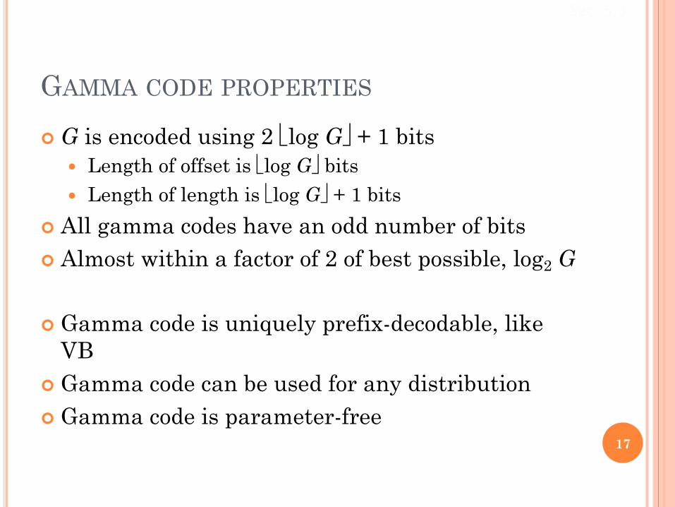
GAMMA CODE PROPERTIES

¢ G is encoded using 2 ëlog Gû + 1 bits� Length of offset is ëlog Gû bits� Length of length is ëlog Gû + 1 bits

¢ All gamma codes have an odd number of bits¢ Almost within a factor of 2 of best possible, log2 G

¢ Gamma code is uniquely prefix-decodable, like VB

¢ Gamma code can be used for any distribution¢ Gamma code is parameter-free

Sec. 5.3

17

GAMMA SELDOM USED IN PRACTICE

¢ Machines have word boundaries – 8, 16, 32, 64 bits� Operations that cross word boundaries are slower

¢ Compressing and manipulating at the granularity of bits can be slow

¢ Variable byte encoding is aligned and thus potentially more efficient

¢ Regardless of efficiency, variable byte is conceptually simpler at little additional space cost

Sec. 5.3

18

RCV1 COMPRESSION

Data structure Size in MBdictionary, fixed-width 11.2dictionary, term pointers into string 7.6with blocking, k = 4 7.1with blocking & front coding 5.9collection (text, xml markup etc) 3,600.0collection (text) 960.0Term-doc incidence matrix 40,000.0postings, uncompressed (32-bit words) 400.0postings, uncompressed (20 bits) 250.0postings, variable byte encoded 116.0postings, g-encoded 101.0

Sec. 5.3

19

INDEX COMPRESSION SUMMARY

¢ We can now create an index for highly efficient Boolean retrieval that is very space efficient

¢ Only 4% of the total size of the collection¢ Only 10-15% of the total size of the text in the

collection¢ However, we’ve ignored positional information¢ Hence, space savings are less for indexes used in

practice� But techniques substantially the same.

Sec. 5.3

20

RESOURCES FOR TODAY’S LECTURE

¢ IIR 5¢ MG 3.3, 3.4.¢ F. Scholer, H.E. Williams and J. Zobel. 2002.

Compression of Inverted Indexes For Fast Query Evaluation. Proc. ACM-SIGIR 2002.� Variable byte codes

¢ V. N. Anh and A. Moffat. 2005. Inverted Index Compression Using Word-Aligned Binary Codes. Information Retrieval 8: 151–166. � Word aligned codes

Ch. 5

21

MORE RESOURCES

¢ K. Kukich. Techniques for automatically correcting words in text. ACM Computing Surveys 24(4), Dec 1992.

¢ Dean, Jeffrey, and Sanjay Ghemawat. MapReduce: simplified data processing on large clusters, OSDI (4) (2004).

22

SCORING, TERMWEIGHTING & VECTOR

SPACE MODEL

RECAP OF LAST LECTURE

¢ Collection and vocabulary statistics: Heaps’ and Zipf’s laws¢ Dictionary compression for Boolean indexes

� Dictionary string, blocks, front coding¢ Postings compression: Gap encoding, prefix-unique codes

� Variable-Byte and Gamma codes

collection (text, xml markup etc) 3,600.0

collection (text) 960.0

Term-doc incidence matrix 40,000.0

postings, uncompressed (32-bit words) 400.0

postings, uncompressed (20 bits) 250.0

postings, variable byte encoded 116.0

postings, γ-encoded 101.0

MB

24

OUTLINE

¢ Ranked retrieval¢ Scoring documents¢ Term frequency¢ Collection statistics¢ Weighting schemes¢ Vector space scoring

25

RANKED RETRIEVAL

¢ Thus far, our queries have all been Boolean.� Documents either match or don’t.

¢ Good for expert users with precise understanding of their needs and the collection.� Also good for applications: Applications can easily

consume 1000s of results.¢ Not good for the majority of users.

� Most users incapable of writing Boolean queries (or they are, but they think it’s too much work).

� Most users don’t want to wade through 1000s of results.¢ This is particularly true of web search.

Ch. 6

26

PROBLEM WITH BOOLEAN SEARCH:FEAST OR FAMINE

¢ Boolean queries often result in either too few (=0) or too many (1000s) results.

¢ Query 1: “standard user dlink 650” → 200,000 hits

¢ Query 2: “standard user dlink 650 no card found”: 0 hits

¢ It takes a lot of skill to come up with a query that produces a manageable number of hits.� AND gives too few; OR gives too many

Ch. 6

27

RANKED RETRIEVAL MODELS

¢ Rather than a set of documents satisfying a query expression, in ranked retrieval, the system returns an ordering over the (top) documents in the collection for a query

¢ Free text queries: Rather than a query language of operators and expressions, the user’s query is just one or more words in a human language

¢ In principle, these are two separate choices here, but in practice, ranked retrieval has normally been associated with free text queries and vice versa

28

FEAST OR FAMINE: NOT A PROBLEM INRANKED RETRIEVAL

¢ When a system produces a ranked result set, large result sets are not an issue� Indeed, the size of the result set is not

an issue� We just show the top k ( ≈ 10) results� We don’t overwhelm the user

� Premise: the ranking algorithm works

Ch. 6

29

SCORING AS THE BASIS OF RANKEDRETRIEVAL

¢ We wish to return the documents in an order most likely to be useful to the searcher

¢ How can we rank-order the documents in the collection with respect to a query?

¢ Assign a score – say in [0, 1] – to each document¢ This score measures how well document and

query “match”.

Ch. 6

30

QUERY-DOCUMENT MATCHING SCORES

¢ We need a way of assigning a score to a query/document pair

¢ Let’s start with a one-term query¢ If the query term does not occur in the document:

score should be 0¢ The more frequent the query term in the

document, the higher the score (should be)¢ We will look at a number of alternatives for this.

Ch. 6

31

TAKE 1: JACCARD COEFFICIENT

¢ Recall from last lecture: A commonly used measure of overlap of two sets A and Bjaccard(A,B) = |A ∩ B| / |A ∪ B|jaccard(A,A) = 1jaccard(A,B) = 0 if A ∩ B = 0

¢ A and B don’t have to be the same size.¢ Always assigns a number between 0 and 1.

Ch. 6

32

QUIZ: JACCARD COEFFICIENT

¢ What is the query-document match score that the Jaccard coefficient computes for each of the two documents below?

¢ Query: ides of march¢ Document 1: caesar died in march¢ Document 2: the long march

Ch. 6

33

ISSUES WITH JACCARD FOR SCORING

¢ It doesn’t consider term frequency (how many times a term occurs in a document)

¢ Rare terms in a collection are more informative than frequent terms. Jaccard doesn’t consider this information

¢ We need a more sophisticated way of normalizing for length

¢ Later in this lecture, we’ll use ¢ . . . instead of |A ∩ B|/|A ∪ B| (Jaccard) for

length normalization.

| B A|/| B A| !"

Ch. 6

34

RECALL: BINARY TERM-DOCUMENTINCIDENCE MATRIX

Antony and Cleopatra Julius Caesar The Tempest Hamlet Othello Macbeth

Antony 1 1 0 0 0 1Brutus 1 1 0 1 0 0Caesar 1 1 0 1 1 1

Calpurnia 0 1 0 0 0 0Cleopatra 1 0 0 0 0 0

mercy 1 0 1 1 1 1

worser 1 0 1 1 1 0

Each document is represented by a binary vector ∈{0,1}|V|

Sec. 6.2

35

TERM-DOCUMENT COUNT MATRICES

¢ Consider the number of occurrences of a term in a document: � Each document is a count vector in ℕv: a column

below

Antony and Cleopatra Julius Caesar The Tempest Hamlet Othello Macbeth

Antony 157 73 0 0 0 0Brutus 4 157 0 1 0 0Caesar 232 227 0 2 1 1

Calpurnia 0 10 0 0 0 0Cleopatra 57 0 0 0 0 0

mercy 2 0 3 5 5 1

worser 2 0 1 1 1 0

Sec. 6.2

36

BAG OF WORDS MODEL

¢ Vector representation doesn’t consider the ordering of words in a document

¢ John is quicker than Mary and Mary is quicker than John have the same vectors

¢ This is called the bag of words model.¢ In a sense, this is a step back: The positional

index was able to distinguish these two documents.

¢ We will look at “recovering” positional information later in this course.

¢ For now: bag of words model 37

TERM FREQUENCY TF

¢ The term frequency tft,d of term t in document d is defined as the number of times that t occurs in d.

¢ We want to use tf when computing query-document match scores. But how?

¢ Raw term frequency is not what we want:� A document with 10 occurrences of the term is more

relevant than a document with 1 occurrence of the term.

� But not 10 times more relevant.¢ Relevance does not increase proportionally with

term frequency.NB: frequency = count in IR 38

LOG-FREQUENCY WEIGHTING

¢ The log frequency weight of term t in d is

¢ 0 → 0, 1 → 1, 2 → 1.3, 10 → 2, 1000 → 4, etc.¢ Score for a document-query pair: sum over terms t

in both q and d:¢ score

¢ The score is 0 if none of the query terms is present in the document.

îíì >+

=otherwise 0,

0 tfif, tflog 1 10 t,dt,d

t,dw

å ÇÎ+=

dqt dt ) tflog (1 ,

Sec. 6.2

39

DOCUMENT FREQUENCY

¢ Rare terms are more informative than frequent terms� Recall stop words

¢ Consider a term in the query that is rare in the collection (e.g., arachnocentric)

¢ A document containing this term is very likely to be relevant to the query arachnocentric

→ We want a high weight for rare terms like arachnocentric.

Sec. 6.2.1

40

DOCUMENT FREQUENCY, CONTINUED

¢ Frequent terms are less informative than rare terms

¢ Consider a query term that is frequent in the collection (e.g., high, increase, line)

¢ A document containing such a term is more likely to be relevant than a document that doesn’t

¢ But it’s not a sure indicator of relevance.¢ In general, we want high positive weights for a

term that appears many times in a doc¢ But lower weights for a frequent term than for

rare terms.¢ We will use document frequency (df) to capture

this.

Sec. 6.2.1

41

IDF WEIGHT

¢ dft is the document frequency of t: the number of documents that contain t� dft is an inverse measure of the informativeness of t� dft £ N (total number of docs)

¢ We define the idf (inverse document frequency) of tby

� We use log (N/dft) instead of N/dft to “dampen” the effect of idf.

)/df( log idf 10 tt N=

It turns out the base of the log is insignificant.

Sec. 6.2.1

42

IDF EXAMPLE, SUPPOSE N = 1 MILLION

term dft idftcalpurnia 1 6

animal 100 4

sunday 1,000 3

fly 10,000 2

under 100,000 1

the 1,000,000 0

There is one idf value for each term t in a collection.

Sec. 6.2.1

)/df( log idf 10 tt N=43

QUIZ: IDF

¢ Why is the idf of a term in a document always finite?

44

)/df( log idf 10 tt N=

EFFECT OF IDF ON RANKING

¢ Does idf have an effect on ranking for one-term queries, like� iPhone?

¢ idf has no effect on ranking one term queries� idf affects the ranking of documents for queries with

at least two terms� For the query capricious person, idf weighting makes

occurrences of capricious count for much more in the final document ranking than occurrences of person.

45

COLLECTION VS. DOCUMENT FREQUENCY

¢ The collection frequency of t is the number of occurrences of t in the collection, counting multiple occurrences.

¢ Example:

Word Collection frequency Document frequencyinsurance 10440 3997

try 10422 8760

Sec. 6.2.1

46

QUIZ: COLLECTION FREQUENCY

¢ Which word is a better search term (and should get a higher weight), and why?

47

Word Collection frequency Document frequencyinsurance 10440 3997

try 10422 8760

TF-IDF WEIGHTING

¢ The tf-idf weight of a term is the product of its tf weight and its idf weight.

¢ Best known weighting scheme in information retrieval� Note: the “-” in tf-idf is a hyphen, not a minus sign!� Alternative names: tf.idf, tf x idf

¢ Increases with the number of occurrences within a document

¢ Increases with the rarity of the term in the collection

Sec. 6.2.2

48

)df/(log)tflog1(w 10,10, tdt Ndt

´+=

SCORE FOR A DOCUMENT GIVEN A QUERY

¢There are many variants� How “tf” is computed (with/without logs)� Whether the terms in the query are also

weighted� …

Score(q,d) = tf.idft,dtÎqÇdå

Sec. 6.2.2

49

BINARY → COUNT → WEIGHT MATRIX

Antony and Cleopatra Julius Caesar The Tempest Hamlet Othello Macbeth

Antony 5.25 3.18 0 0 0 0.35Brutus 1.21 6.1 0 1 0 0Caesar 8.59 2.54 0 1.51 0.25 0

Calpurnia 0 1.54 0 0 0 0Cleopatra 2.85 0 0 0 0 0

mercy 1.51 0 1.9 0.12 5.25 0.88

worser 1.37 0 0.11 4.15 0.25 1.95

Each document is now represented by a real-valued vector of tf-idf weights ∈ R|V|

Sec. 6.3

50

DOCUMENTS AS VECTORS

¢ So we have a |V|-dimensional vector space¢ Terms are axes of the space¢ Documents are points or vectors in this space¢ Very high-dimensional: tens of millions of

dimensions when you apply this to a web search engine

¢ These are very sparse vectors - most entries are zero.

Sec. 6.3

51

QUERIES AS VECTORS

¢ Key idea 1: Do the same for queries: represent them as vectors in the space

¢ Key idea 2: Rank documents according to their proximity to the query in this space

¢ proximity = similarity of vectors¢ proximity ≈ inverse of distance¢ Recall: We do this because we want to get away

from the you’re-either-in-or-out Boolean model.¢ Instead: rank more relevant documents higher

than less relevant documents

Sec. 6.3

52

FORMALIZING VECTOR SPACE PROXIMITY

¢ First cut: distance between two points� ( = distance between the end points of the two

vectors)¢ Euclidean distance?¢ Euclidean distance is a bad idea . . .¢ . . . because Euclidean distance is large for

vectors of different lengths.

Sec. 6.3

53

WHY DISTANCE IS A BAD IDEA

The Euclidean distance between qand d2 is large even though thedistribution of terms in the query q and the distribution ofterms in the document d2 arevery similar.

Sec. 6.3

54

FROM EUCLIDEAN TO ANGLE DISTANCE

¢ Thought experiment: take a document d and append it to itself. Call this document d′.

¢ “Semantically” d and d′ have the same content¢ The Euclidean distance between the two

documents can be quite large¢ The angle between the two documents is 0,

corresponding to maximal similarity.

¢ Key idea: Rank documents according to angle with query.

Sec. 6.3

55

FROM ANGLES TO COSINES

¢ The following two notions are equivalent.� Rank documents in decreasing order of the angle

between query and document� Rank documents in increasing order of

cosine(query,document)¢ Cosine is a monotonically decreasing function for

the interval [0o, 180o]

Sec. 6.3

56

FROM ANGLES TO COSINES

Sec. 6.3

57¢ But how – and why – should we be computing cosines?

LENGTH NORMALIZATION

¢ A vector can be (length-) normalized by dividing each of its components by its length – for this we use the L2 norm:

¢ Dividing a vector by its L2 norm makes it a unit (length) vector (on surface of unit hypersphere)

¢ Effect on the two documents d and d′ (d appended to itself) from earlier slide: they have the same unit vectors after length-normalization.� Long and short documents now have comparable

weights

å=i ixx 2

2

!

Sec. 6.3

58

COSINE(QUERY,DOCUMENT)

ååå

==

==•=•

=V

i iV

i i

V

i ii

dq

dq

dd

qq

dqdqdq

12

12

1),cos( !

!

!

!

!!

!!!!

Dot product Unit vectors

qi is the tf-idf weight of term i in the querydi is the tf-idf weight of term i in the document

cos(q,d) is the cosine similarity of q and d … or,equivalently, the cosine of the angle between q and d.

Sec. 6.3

59

60

COSINE FOR LENGTH-NORMALIZEDVECTORS

¢ For length-normalized vectors, cosine similarity is simply the dot product (or scalar product):

for q, d length-normalized.!!

cos("!q ,"!d ) ="!q •"!d = qidii=1

Vå

61

COSINE SIMILARITY ILLUSTRATED

62

COSINE SIMILARITY AMONGST 3 DOCUMENTS¢ How similar are

the novels?¢ SaS: Sense and

Sensibility¢ PaP: Pride and

Prejudice¢ WH: Wuthering

Heights

63

term SaS PaP WH

affection 115 58 20

jealous 10 7 11

gossip 2 0 6

wuthering 0 0 38

Term frequencies (counts)

Note: To simplify this example, we don’t do idfweighting.

3 DOCUMENTS EXAMPLE CONTD.

Log frequency weighting

term SaS PaP WHaffection 3.06 2.76 2.30jealous 2.00 1.85 2.04gossip 1.30 0 1.78wuthering 0 0 2.58

After length normalization

term SaS PaP WHaffection 0.789 0.832 0.524jealous 0.515 0.555 0.465gossip 0.335 0 0.405wuthering 0 0 0.588

cos(SaS,PaP) ≈0.789 ! 0.832 + 0.515 ! 0.555 + 0.335 ! 0.0 + 0.0 ! 0.0 ≈ 0.94cos(SaS,WH) ≈ 0.79cos(PaP,WH) ≈ 0.69

Sec. 6.3

64

QUIZ: NOVELS

¢Why do we have cos(SaS,PaP) > cos(SaS,WH)?

¢Give one simple reason.

65

COMPUTING COSINE SCORES

Sec. 6.3

66

TF-IDF WEIGHTING HAS MANY VARIANTS

‘n’, ‘l’, ‘a’, ‘t’, ‘p’, etc. are acronyms for weight schemes.

Quiz: Why is the base of the log in idf insignificant?

Sec. 6.4

67

WEIGHTING MAY DIFFER IN QUERIES VSDOCUMENTS

¢ Many search engines allow for different weightings for queries vs. documents

¢ SMART Notation: denotes the combination in use in an engine, with the notation ddd.qqq, using the acronyms from the previous table

¢ A very standard weighting scheme is: lnc.ltc¢ Document: logarithmic tf (l as first character), no idf

and cosine normalization

¢ Query: logarithmic tf (l in leftmost column), idf (t in second column), no normalization …

A bad idea?

Sec. 6.4

68

TF-IDF EXAMPLE: LNC.LTC

Term Query Document Prodtf-

rawtf-wt df idf tfidf

wtn’liz

etf-raw tf-wt tfidf

wtn’liz

eauto 0 0 5000 2.3 0 0 1 1 1 0.52 0best 1 1 50000 1.3 1.3 0.34 0 0 0 0 0car 1 1 10000 2.0 2.0 0.52 1 1 1 0.52 0.27insurance 1 1 1000 3.0 3.0 0.78 2 1.3 1.3 0.68 0.53

Document: car insurance auto insuranceQuery: best car insurance

Exercise: what is N, the number of docs?

Score = 0+0+0.27+0.53 = 0.8

Doc vector length =

12 +02 +12 +1.32 »1.92

Sec. 6.4

69

SUMMARY – VECTOR SPACE RANKING

¢ Represent the query as a weighted tf-idf vector¢ Represent each document as a weighted tf-idf vector¢ Compute the cosine similarity score for the query

vector and each document vector¢ Rank documents with respect to the query by score¢ Return the top K (e.g., K = 10) to the user

70

RESOURCES FOR TODAY’S LECTURE

¢ IIR 6.2 – 6.4.3

¢ http://www.miislita.com/information-retrieval-tutorial/cosine-similarity-tutorial.html� Term weighting and cosine similarity tutorial for

SEO folk!

Ch. 6

71