Independent Component Analysis Enhancements for Source

University of Kentucky University of Kentucky

UKnowledge UKnowledge

Theses and Dissertations--Electrical and Computer Engineering Electrical and Computer Engineering

2013

Independent Component Analysis Enhancements for Source Independent Component Analysis Enhancements for Source

Separation in Immersive Audio Environments Separation in Immersive Audio Environments

Yue Zhao University of Kentucky, [email protected]

Right click to open a feedback form in a new tab to let us know how this document benefits you. Right click to open a feedback form in a new tab to let us know how this document benefits you.

Recommended Citation Recommended Citation Zhao, Yue, "Independent Component Analysis Enhancements for Source Separation in Immersive Audio Environments" (2013). Theses and Dissertations--Electrical and Computer Engineering. 34. https://uknowledge.uky.edu/ece_etds/34

This Master's Thesis is brought to you for free and open access by the Electrical and Computer Engineering at UKnowledge. It has been accepted for inclusion in Theses and Dissertations--Electrical and Computer Engineering by an authorized administrator of UKnowledge. For more information, please contact [email protected].

http://uknowledge.uky.edu/

http://uknowledge.uky.edu/

https://uknowledge.uky.edu/

https://uknowledge.uky.edu/ece_etds

https://uknowledge.uky.edu/ece_etds

https://uknowledge.uky.edu/ece

https://uky.az1.qualtrics.com/jfe/form/SV_9mq8fx2GnONRfz7

mailto:[email protected]

STUDENT AGREEMENT: STUDENT AGREEMENT:

I represent that my thesis or dissertation and abstract are my original work. Proper attribution

has been given to all outside sources. I understand that I am solely responsible for obtaining

any needed copyright permissions. I have obtained and attached hereto needed written

permission statements(s) from the owner(s) of each third-party copyrighted matter to be

included in my work, allowing electronic distribution (if such use is not permitted by the fair use

doctrine).

I hereby grant to The University of Kentucky and its agents the non-exclusive license to archive

and make accessible my work in whole or in part in all forms of media, now or hereafter known.

I agree that the document mentioned above may be made available immediately for worldwide

access unless a preapproved embargo applies.

I retain all other ownership rights to the copyright of my work. I also retain the right to use in

future works (such as articles or books) all or part of my work. I understand that I am free to

register the copyright to my work.

REVIEW, APPROVAL AND ACCEPTANCE REVIEW, APPROVAL AND ACCEPTANCE

The document mentioned above has been reviewed and accepted by the student’s advisor, on

behalf of the advisory committee, and by the Director of Graduate Studies (DGS), on behalf of

the program; we verify that this is the final, approved version of the student’s dissertation

including all changes required by the advisory committee. The undersigned agree to abide by

the statements above.

Yue Zhao, Student

Dr. Kevin D. Donohue, Major Professor

Dr. Cai-Cheng Lu, Director of Graduate Studies

INDEPENDENT COMPONENT ANALYSIS

ENHANCEMENTS FOR SOURCE SEPARATION

IN IMMERSIVE AUDIO ENVIRONMENTS

THESIS

A thesis submitted in partial fulfillment of the

requirements for the degree of Master of Science in

Electrical Engineering in the College of Engineering

at the University of Kentucky

By

Yue Zhao

Lexington, Kentucky

Director: Dr. Kevin D. Donohue, Professor of Electrical and Computer Engineering

Lexington, Kentucky

2013

Copyright© Yue Zhao 2013

ABSTRACT OF THESIS




In immersive audio environments with distributed microphones, Independent Component

Analysis (ICA) can be applied to uncover signals from a mixture of other signals and

noise, such as in a cocktail party recording. ICA algorithms have been developed for

instantaneous source mixtures and convolutional source mixtures. While ICA for

instantaneous mixtures works when no delays exist between the signals in each mixture,

distributed microphone recordings typically result various delays of the signals over the

recorded channels. The convolutive ICA algorithm should account for delays; however, it

requires many parameters to be set and often has stability issues. This thesis introduces

the Channel Aligned FastICA (CAICA), which requires knowledge of the source distance

to each microphone, but does not require knowledge of noise sources. Furthermore, the

CAICA is combined with Time Frequency Masking (TFM), yielding even better SOI

extraction even in low SNR environments. Simulations were conducted for ranking

experiments tested the performance of three algorithms: Weighted Beamforming (WB),

CAICA, CAICA with TFM. The Closest Microphone (CM) recording is used as a

reference for all three. Statistical analyses on the results demonstrated superior

performance for the CAICA with TFM. The algorithms were applied to experimental

recordings to support the conclusions of the simulations. These techniques can be

deployed in mobile platforms, used in surveillance for capturing human speech and

potentially adapted to biomedical fields.

Multimedia Elements Used: WAV (.wav)

KEYWORDS: Blind Source Separation, Independent Component Analysis, Audio Signal

Processing, Convolutional Source Separation, Information Theory

Yue Zhao

10/01/2013




By

Yue Zhao

Kevin D. Donohue

Director of Thesis

Cai-Cheng Lu

Director of Graduate Studies

10/01/2013

To my loving parents, dear teachers, friends and colleagues

iii

ACKNOWLEDGMENTS

I would like to give my sincere and deep thanks to my thesis advisor, Dr. Kevin

Donohue. I am very grateful for his guidance and advice throughout the thesis process

as well as his invaluable mentoring. Without him, this thesis wouldn’t be complete.

Thanks to Dr. Sen-ching Cheung and Dr. Grzegorz Wasilkowski for taking their valuable

time to sit in on my thesis defense and offering me valuable input.

I would love to thank all the members in the Audio Systems Lab for their meaningful

discussions and support: Jingjing, Harikrishnan, Ryan, Jordan, Kirstin and Josh. I’d like

to thank all other members in the VISCENTER for cutting edge research and their

willingness to share. I am grateful for all the professors that taught me in University of

Kentucky. This thesis work was supported by the Elise White Boyd Graduate Fellowship.

I appreciate for the funding that made this thesis possible.

Thanks to my loving parents Liangfeng and Wencheng for their understandings of the

all the electronic toys, alarm clocks, watches etc. that I opened and tried to put back

together due to my curiosity for technology. This curiosity multiplied and eventually

inspired me to choose electrical engineering as my major. Thanks to my mom for

company for all those years and days of erhu practice, through which I developed a

close bond with music. Thanks to my parents for their support and encouragement so

that I am able to chase my dreams in engineering. I also appreciate the support of my

loving friends Chrys, Jimmy, Yuanjing and Anca.

http://uknowledge.uky.edu/do/search/?q=author_lname%3A%22Unnikrishnan%22%20author_fname%3A%22Harikrishnan%22&start=0&context=1674591

iv

TABLE OF CONTENTS

ACKNOWLEDGMENTS ................................................................................................. iii

LIST OF TABLES ............................................................................................................ vii

LIST OF FIGURES ......................................................................................................... viii

LIST OF FILES ................................................................................................................ xii

Chapter 1 : Introduction and Literature Review .............................................................. 1

1.1 A Brief History for Blind Source Separation and Independent Component Analysis

......................................................................................................................................... 1

1.2 BSS/ ICA Research and Thesis Motivation .............................................................. 2

1.3 ICA in Audio Signal Processing ............................................................................... 2

1.4 Current Research on BSS and their Literature Review ............................................. 4

1.4.1 Using one microphone to separate singing voice ............................................... 5

1.4.2 Blind Separation of Convolutive Mixtures using Spatio-Temporal FastICA

Algorithms ................................................................................................................... 7

1.4.3 Adaptive time-domain blind separation of speech signals ................................. 9

1.4.4 DOA Estimation for Multiple Sparse Sources with Arbitrarily Arranged

Multiple Sensors ........................................................................................................ 11

1.4.5 The Signal Separation Evaluation Campaign (2007–2010): Achievements and

Remaining Challenges ............................................................................................... 13

Chapter 2 : FastICA ....................................................................................................... 16

2.1 ICA Algorithm and its Literature Review ............................................................... 16

2.1.1 ICA Basic Model .............................................................................................. 17

2.2 Preprocessing steps for BSS/ICA ............................................................................ 19

2.2.1 Filtering ............................................................................................................ 19

2.2.2 Preprocessing via Dimension Reduction through Principal Component

Analysis ..................................................................................................................... 20

2.2.3 ICA Preprocessing through Whitening ............................................................. 21

v

2.3 ICA/FastICA Main Algorithm ................................................................................ 21

2.3.1 FastICA for one computational unit ................................................................. 23

2.3.2 FastICA for several computational units .......................................................... 23

2.4 Noisy ICA model .................................................................................................... 25

2.5 Limitation of ICA/FastICA ..................................................................................... 25

2.6 FastICA Experiment Setup...................................................................................... 26

2.6.1 FastICA Parameter Configuration Procedures ................................................. 26

2.6.2 Experiment Setup ............................................................................................. 28

2.6.3 Conclusions ...................................................................................................... 32

Chapter 3: Convolutive BSS ......................................................................................... 33

3.1 Convolutive BSS Algorithm and its Literature Review .......................................... 33

3.2 Using Convolutive BSS to model the Cocktail Party Scenario .............................. 35

3.3 Comparison and contrast between the instantaneous and convolutional ICA

approaches ..................................................................................................................... 37

3.4 Convolutive BSS Experiment Setup ....................................................................... 40

3.5 Problems Encountered When Using Convolutional BSS Toolbox ......................... 49

Chapter 4: Channel Aligned Fast ICA .......................................................................... 53

4.1 CAICA Description ................................................................................................. 54

4.2 Closest Microphone(CM) recordings ..................................................................... 54

4.3 Weighted Beamforming (WB): ............................................................................... 55

4.4 Time Frequency Masking (TFM) ............................................................................ 55

4.5 CAICA with TF Masking ........................................................................................ 55

Chapter 5: Simulation Experiment ............................................................................... 56

5.1 Simulation Setup ..................................................................................................... 56

5.2 Simulation Procedures............................................................................................. 58

5.3 Experiment Approaches and Descriptions .............................................................. 62

5.4 Statistical Analysis .................................................................................................. 66

5.5 Conclusions ............................................................................................................. 68

Chapter 6: Algorithm Validation .................................................................................. 69

vi

6.1 Experiments Setup................................................................................................... 71

6.2 Processing Procedures ............................................................................................. 74

6.3 Results, Comments and Remarks ............................................................................ 90

Chapter 7: Final Conclusions and Future Work ........................................................... 93

7.1 Conclusions ............................................................................................................. 93

7.2 Future Work ............................................................................................................ 94

References ......................................................................................................................... 96

Vita .................................................................................................................................... 98

vii

LIST OF TABLES

Table 3.1: Comparison Amongst Standard Linear ICA, BSS, and ConvolutiveBSS.…...37

Table 3.2: Fixed parameters in the experiment……………………………….………….41

Table 3.3: Parameters in the 16 simulations……………………………………………..41

Table 3.4: Speaker locations in meters for furthest speaker apart is 3.5 m…............,.....43

Table 3.5: Microphone locations in meters for furthest speaker apart is 3.5 m……....…43

Table 3.6: Speaker locations in meters for furthest speaker apart is 0.25 m ………..…..44

Table 3.7: Microphone locations in meters for furthest speaker apart is 0.25 m ….....…44

Table 3.8: Values used in ConvBSS separation process………………………………....46

Table 3.9: Parameter values to validate the Convolutional BSS Performance…………..50

Table 5.1: Speaker Locations in meters for this setup …………….…………………….57

Table 5.2: Microphone Locations in meters for this setup ………………….…………..57

Table 5.3: Test_Laboratory Member A Sound Track Ranking………………………….65

Table 5.4: Algorithm Ranking_ Laboratory Member A’s Score………………………...66

Table 5.5: Statistical Analysis……………………………………………………….67, 68

Table 6.1: Experiment Settings…………………………………………………………..71

Table 6.2: Speaker of Interest (SOI) Mean Coordinates in Meters……………………...73

Table 6.3: Microphone Coordinates in Meters …............................................................73

viii

LIST OF FIGURES

Figure 1.1 GMM- Based Separation Scheme from Ozerov, A.; Philippe, P.; Gribonval, R.;

Bimbot, F., "One microphone singing voice separation using source-adapted models," [11]

............................................................................................................................................. 5

Figure 1.2 Source-adapted separation scheme from Ozerov, A.; Philippe, P.; Gribonval,

R.; Bimbot, F., "One microphone singing voice separation using source-adapted models,"

[11] ...................................................................................................................................... 6

Figure 1.3 Block Diagram of the Combined Separation and Signal Reconstruction System

from from Douglas, S.C.; Gupta, M.; Sawada, H.; Makino, S., "Spatio–Temporal

FastICA Algorithms for the Blind Separation of Convolutive Mixtures," [13] ................. 9

Figure 1.4 Structure of the proposed method from Araki, S., Sawada, H., Mukai, R., &

Makino, S. (2011). DOA estimation for multiple sparse sources with arbitrarily arranged

multiple sensors [18] ......................................................................................................... 12

Figure 2.1: ICA Procedures Block Diagram ..................................................................... 16

Figure 2.2: Channel 2 Mixture Channel ........................................................................... 29

Figure 2.3: Source Man1................................................................................................... 29

Figure 2.4: Source Man2................................................................................................... 30

Figure 2.5: Source woman1 .............................................................................................. 30

Figure 2.6: Source woman2 .............................................................................................. 31

Figure 3.1: Overall ICA model ......................................................................................... 37

Figure 3.2: Furthest microphone apart is 3.5m; furthest speaker apart is 3.5m ................ 42

Figure 3.3: Top view of figure 3.2 .................................................................................... 42

Figure 3.4: Furthest microphone apart is 3.5 m, furthest speaker apart is 0.25 m ............ 43

Figure 3.5: Top view of figure 3.4 .................................................................................... 44

Figure 3.6: 3.5mic_3.5speakers_lowrev random selected four out of eight microphone

recordings before using ConvBSS method ....................................................................... 47

Figure 3.7: 3.5mic_3.5speakers_lowrev_highfc_0.5antin0.5causalfilt_convsepartion with

every color represents one underlying source after separation using ConvBSS method . 47


recordings before using ConvBSS method ....................................................................... 48

ix

Figure 3.9: 0.25mic_3.5speakers_lowrev_highfc_0.5antin0.5causalfilt_convsepartion

with every color represents one underlying source after separation using ConvBSS

method............................................................................................................................... 49

Figure 5.1: Microphones and Speakers 3-D coordinates .................................................. 56

Figure 5.2: Microphones and Speakers 3-D coordinates .................................................. 57

Figure 5.3: Normalized SOI (man3) ................................................................................. 59

Figure 5.4: SOI(man3) closest microphone 3 ................................................................... 60

Figure 5.5: SOI(man3) weighted beamforming ................................................................ 60

Figure 5.6: SOI (man3) channel adjusted fastICA SOI channel 7 .................................... 61

Figure 5.7: SOI(man3)channel adjusted fastICA with time frequency masking .............. 61

Figure 5.8: All wave forms for comparison ...................................................................... 62

Figure 5.9: Audacity user interface for one experiment ................................................... 64

Figure 6.1: Cage side with Linear Microphone array, a couple of speakers, and absorptive

acoustic treatment ............................................................................................................. 69

Figure 6.2: Cage with Speakers side view ........................................................................ 70

Figure 6.3: Cage with Speakers back view ....................................................................... 70

Figure 6.4: 3-D View of the microphone Locations and mean Speaker Location ........... 72

Figure 6.5: Labeled 16 Microphones and Speaker of Interest Mean Location Top view 73

Figure 6.6: SNR=2 dB, pure SOI at closest microphone waveform ................................. 75

Figure 6.7: SNR=2 dB, pure SOI at closest microphone filtered waveform .................... 75

Figure 6.8: SNR=2 dB, cocktail party at closest microphone waveform ......................... 76

Figure 6.9: SNR=2 dB, cocktail party weighted beam forming waveform ...................... 76

Figure 6.10: SNR=2 dB, cocktail party channel adjusted fastICA SOI channel waveform

........................................................................................................................................... 77

Figure 6.11: SNR = 2 dB, cocktail party channel adjusted fastICA with 16 channel TFM

waveform .......................................................................................................................... 77

Figure 6.12: SNR = 2 dB, cocktail party channel adjusted fastICA with 4 channel (with

one SOI, 3 hand-picked interferences channels) TFM waveform .................................... 78

Figure 6.13: SNR = 2 dB, waveform comparisons ........................................................... 78

x

Figure 6.14: SNR = 2 dB, filtered pure SOI, channel adjusted fastICA with16-channel

time frequency masking, channel adjusted fastICA with4-channel time frequency

masking waveform comparisons ....................................................................................... 79

Figure 6.15: SNR=0 dB, pure SOI at closest microphone waveform ............................... 80

Figure 6.16: SNR=0 dB, pure SOI at closest microphone filtered waveform .................. 80

Figure 6.17: SNR=0 dB, cocktail party at closest microphone waveform ....................... 81

Figure 6.18: SNR=0 dB, cocktail party weighted beam forming waveform .................... 81


........................................................................................................................................... 82

Figure 6.20: SNR = 0 dB, cocktail party channel adjusted fastICA with 16 channel time

frequency masking waveform ........................................................................................... 82


one SOI, 3 hand-picked interferences channels) time frequency masking waveform ...... 83

Figure 6.22: SNR = 0 dB, waveform comparisons ........................................................... 83

Figure 6.23: SNR = 0 dB, filtered pure SOI, channel adjusted fastICA with16 channel

time frequency masking, channel adjusted fastICA with16 channel time frequency

masking waveform comparisons ....................................................................................... 84

Figure 6.24: SNR=-10 dB, pure SOI at closest microphone waveform ........................... 85

Figure 6.25: SNR=-10 dB, pure SOI at closest microphone filtered waveform ............... 85

Figure 6.26: SNR=-10 dB, cocktail party at closest microphone waveform .................... 86

Figure 6.27: SNR=-10 dB, cocktail party weighted beam forming waveform ................. 86

Figure 6.28: SNR=-10 dB, cocktail party channel adjusted fastICA SOI channel

waveform .......................................................................................................................... 87

Figure 6.29: SNR = -10 dB, cocktail party channel adjusted fastICA with 16 channel time

frequency masking waveform ........................................................................................... 87

Figure 6.30: SNR = -10 dB, cocktail party channel adjusted fastICA with 4 channel (with






xi

Figure 6.33: SNR = -10 dB, waveform comparisons ....................................................... 89

Figure 6.34: SNR = -10 dB, filtered pure SOI, channel adjusted fastICA with16-channel,

4-channel, 6-channel, 8-channel time frequency masking waveform comparisons ......... 90

xii

LIST OF FILES

Channel 2 Mixure Channel.wav…………………………………………………1.32 MB

Filtered and normalized man1 waveform.wav…………………………….…….1.32 MB

Instantaneous Mixture After FastICA normalized waveform for man1.wav……1.32 MB

Filtered and normalized woman2 waveform.wav……………………………….1.32 MB

Instantaneous Mixture After FastICA normalized waveform for woman2.wav...1.32 MB

3.5mic_3.5speakers_lowrev_sigout_channel1.wav……………………………....314 KB

3.5mic_3.5speakers_lowrev_sigout_channel5.wav……………………………....314 KB

3.5mic_3.5speakers_lowrev_highfc_fastica_sep_1.wav…………………………314 KB

3.5mic_3.5speakers_lowrev_highfc_fastica_sep_2.wav………………………....314 KB



3.5mic_3.5speakers_lowrev_sigout_channel3.wav…………………………...….314 KB

3.5mic_3.5speakers_lowrev_sigout_channel6.wav...…………………………….314 KB

3.5mic_3.5speakers_lowrev_highfc_0.5antin0.5causalfilt_convsep_1.wav……...314 KB

3.5mic_3.5speakers_lowrev_highfc_0.5antin0.5causalfilt_convsep_2.wav...…....314 KB



nman2.wav……………………………………………………………………….1.48 MB

nman3.wav……………………………………………………………………….1.48 MB

nman4.wav……………………………………………………………………….1.48 MB

nwoman1.wav………………………………………………………………...….1.48 MB

4spe8mic1pwspeakerman3soi_sp1_norev_simulated_closestmic3.wav………...1.51 MB

4spe8mic1pwspeakerman3soi_sp1_norev_wbeamformed.wav………………....1.51 MB

4spe8mic1pwspeakerman3soi_sp1_norev_channeladjusted

_fastICA_soi_channel7.wav…………………………………………......1.51 MB

4spe8mic1pwspeakerman3soi_sp1_norev_channeladjusted

_fastICA_aftfmasking.wav………............................................................1.53 MB

2SNR_pure soi closest mic channel.wav………………………………………...1.05 MB

2SNR_pure soi closest mic filtered channel.wav………………………………..1.05 MB

xiii

2SNR_Cocktail Party_closestmic2.wav………………………………....………1.05 MB

2SNR_Cocktail Party_wbeamformed.wav………………………………………1.05 MB

2SNR_Cocktail Party_channeladjusted_fastICA_soi_channel14.wav………….1.05 MB

2SNR_Cocktail Party_channeladjusted_fastICA_aftfmasking.wav…………….1.05 MB

2SNR_Cocktail Party_channeladjusted_fastICA_aftfmasking_4 channels……..1.05 MB

-10SNR_pure soi closest mic channel.wav……………………………………...1.05 MB

-10SNR_pure soi closest mic filtered channel.wav………………………….…..1.05 MB

-10SNR_Cocktail Party_closestmic2.wav…………………………………….…1.05 MB

-10SNR_Cocktail Party_wbeamformed.wav……………………………………1.05 MB

-10SNR_Cocktail Party_channeladjusted_fastICA_soi_channel12.wav……….1.05 MB

-10SNR_Cocktail Party_channeladjusted_fastICA_aftfmasking.wav………….1.05 MB

-10SNR_Cocktail Party_channeladjusted_fastICA_aftfmasking_4 channels…...1.05 MB



ICA Enhancements for Source Separation_Thesis_Yue_Final Draft.pdf………...2.1 MB

1

Chapter 1 : Introduction and Literature Review

1.1 A Brief History for Blind Source Separation and Independent Component

Analysis

In digital signal processing, one goal is to recover the original signals from the signal

mixtures, and this process is referred to as Source Separation (SS). A typical scenario for

source separation is the cocktail party scenario where we have multiple speakers,

background music and noise, and we only know the mixtures, but we try to estimate or

even reconstruct the original source of interest (SOI) from the sound mixtures recorded

by microphones [1].

Blind Source Separation (BSS), also referred to as Blind Signal Separation, is a type of

Source Separation (SS) where we have little or no prior knowledge of the sources and the

mixing system. Many methods are used for BSS. The basic methods are Principal

Component Analysis, Singular Value Decomposition, Independent Component Analysis,

Dependent Component Analysis, Non-negative Matrix Factorization, Low-complexity

Coding and Decoding, Stationary Subspace Analysis, and Common Spatial Pattern.

Depending on the kind of source separation problem and the kind of mixing system

involved, we may combine a few of these algorithms for processing mixed data in order

to get optimized separation results. BSS originated with audio processing due to audio

signals’ spatial feature, but can also be applied to image processing, biomedical data,

economic analysis, telecommunications, etc. In this thesis, the research is focused on BSS

in audio environment signal processing [1, 2].

Independent Component Analysis (ICA) is a blind source separation and is one of the

state-of-the-art topics in signal processing, biomedical fields, telecommunications, etc.

Independent Component Analysis (ICA) is a special case of the Blind Source Separation

and this algorithm’s premise is the independent feature of source signals. ICA can

analyze and uncover hidden factors from a set of signals. In the audio signal environment,

the data signals are assumed to be linear or nonlinear mixtures of some unknown latent

source signals, and the mixing system is assumed to be unknown. The latent signals are

2

assumed to be non-Gaussian and mutually independent, and these latent signals are

referred to as the independent components of the observed signal data. Processing the

observed data through BSS/ICA, we can get these independent components, referred to as

sources [1].

1.2 BSS/ ICA Research and Thesis Motivation

Early acoustic source separation systems relied on fixed or adaptive beamforming, and

these techniques are still in use today. Beamforming is a mature technique, and it has

been deployed in commercial products such as cell phones and other electronics to

separate the sources of interest [3]. These methods require prior knowledge such as the

relative positions of the microphones and target source or time intervals during which the

target source is inactive. In our lab, beamforming takes a very long processing time,

requires the location coordinates of the sources to perform separation, and the

beamforming algorithm requires a large number of microphones for good separation

results.

In reality, prior knowledge is rarely available, so we need to consider BSS. Blind Source

Separation (BSS) requires little to no prior knowledge of the sources and/or the mixing

process, does not need nearly as many microphones to perform separation, does not take

nearly as long to perform separation, and theoretically does not need the locations of the

microphones to perform separation, but the layout of the microphones affect the

separation results with related toolbox. Due to the convenience and advantages of the

ICA and BSS, this thesis aims at exploring the feasibility of the ICA and BSS algorithms

in audio environments. Later on, this thesis also explores enhancements of the ICA for

source separation in immersive audio environments.

1.3 ICA in Audio Signal Processing

Two techniques that use BSS for audio separations are convolutive independent

component analysis (convolutive ICA) and sparse component analysis (SCA). These two

techniques characterize real-world audio mixtures and summarize the performance of

existing systems for such mixtures. But these two strategies face permutation alignment

problems.

3

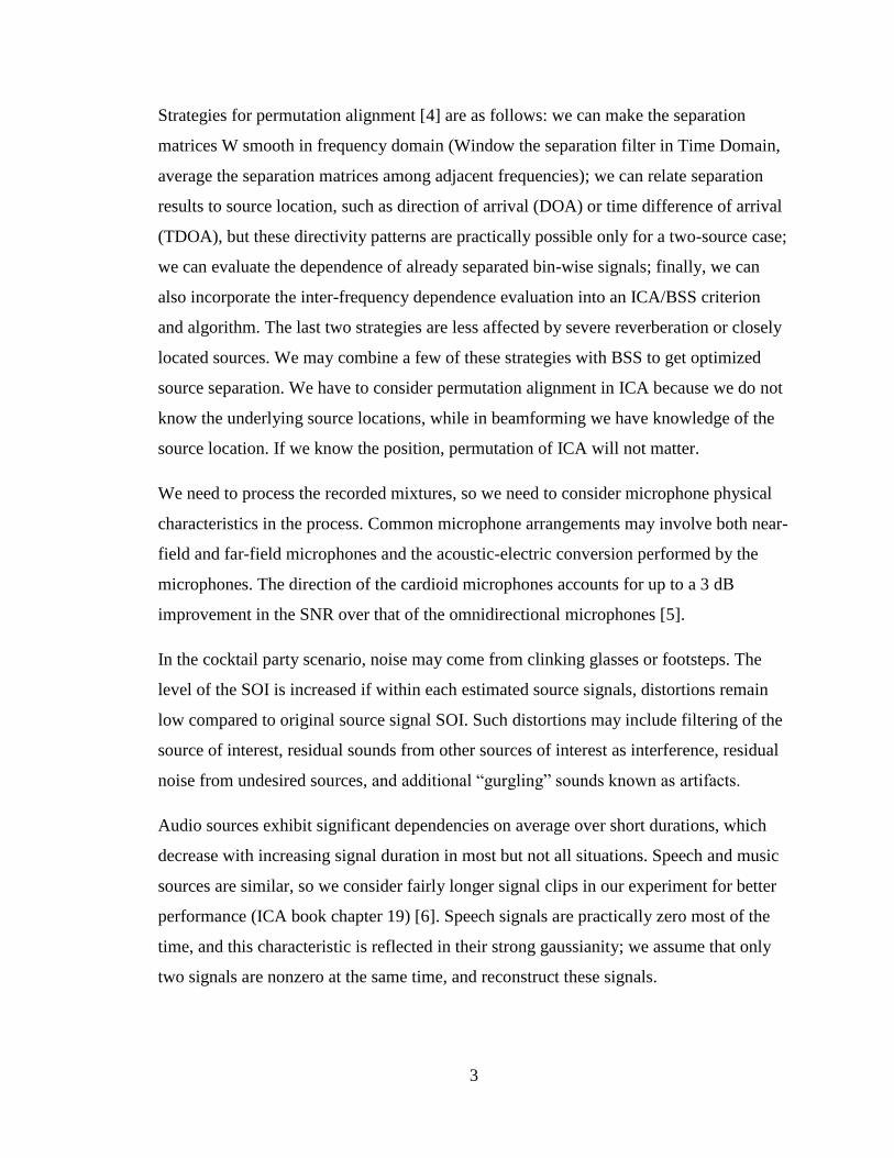
Strategies for permutation alignment [4] are as follows: we can make the separation

matrices W smooth in frequency domain (Window the separation filter in Time Domain,

average the separation matrices among adjacent frequencies); we can relate separation

results to source location, such as direction of arrival (DOA) or time difference of arrival

(TDOA), but these directivity patterns are practically possible only for a two-source case;

we can evaluate the dependence of already separated bin-wise signals; finally, we can

also incorporate the inter-frequency dependence evaluation into an ICA/BSS criterion

and algorithm. The last two strategies are less affected by severe reverberation or closely

located sources. We may combine a few of these strategies with BSS to get optimized

source separation. We have to consider permutation alignment in ICA because we do not

know the underlying source locations, while in beamforming we have knowledge of the

source location. If we know the position, permutation of ICA will not matter.

We need to process the recorded mixtures, so we need to consider microphone physical

characteristics in the process. Common microphone arrangements may involve both near-

field and far-field microphones and the acoustic-electric conversion performed by the

microphones. The direction of the cardioid microphones accounts for up to a 3 dB

improvement in the SNR over that of the omnidirectional microphones [5].

In the cocktail party scenario, noise may come from clinking glasses or footsteps. The

level of the SOI is increased if within each estimated source signals, distortions remain

low compared to original source signal SOI. Such distortions may include filtering of the

source of interest, residual sounds from other sources of interest as interference, residual

noise from undesired sources, and additional “gurgling” sounds known as artifacts.

Audio sources exhibit significant dependencies on average over short durations, which

decrease with increasing signal duration in most but not all situations. Speech and music

sources are similar, so we consider fairly longer signal clips in our experiment for better

performance (ICA book chapter 19) [6]. Speech signals are practically zero most of the

time, and this characteristic is reflected in their strong gaussianity; we assume that only

two signals are nonzero at the same time, and reconstruct these signals.

4

Speech signals consist of a sequence of phones; and it consist of a period, noisy or

transient sounds. Audio sources are generally sparse in the time-frequency domain; in the

time domain, speech sources are generally sparse, but only some music sources are sparse.

Convolutive ICA separates the sources by convolving the mixture signals with

multichannel FIR unmixing filters by maximizing some contrast function. Interference

cancellation improves when the number of notches or their spatial width increases; this

means increasing the number of microphones or the length of the unmixing filters. It will

result in worse performance if sources are less stationary; this happens because

interference must then be canceled over a range of positions even within a short duration.

Also we can only employ the Convolutive ICA method for determined audio sources.

SIRI decreases when the microphones have close locations. Room recordings and car

recordings show that when microphone spacing is smaller, it has larger performance

degradation. But when running experiments on the signals recorded when playing a

speech source through the loudspeaker situated at the driver’s head position are added to

real noise recordings made in a moving car with the same microphone arrays,

performance is better when microphones are closer. The best SIRI obtained for these

mixtures was about 2 dB, which is low communication quality [6].

Separation performance over stereo mixtures dramatically decreases with 1) increasing

reverberation time, 2) decreasing microphone distance, and 3) diffuse interfering sources.

1.4 Current Research on BSS and their Literature Review

Depending on whether the system is under-determined or over-determined, meaning or

we have less microphones than speakers or we have more microphones than speakers,

and also depending on the number of microphones and/ or speakers we have, we can

deploy different BSS algorithms for good separation results.

In the Generative Topographic Mapping (GTM) algorithm, we have mutually similar

impulse (delta) functions that are equispaced on a rectangular grid that are used to model

the discrete uniform density in the space of latent variables, or the joint density of the

sources in our case. GTM is based on a generative approach that starts by assuming a

5

model for the latent variables, in our case [7]. Bayesian learning solves trade-off between

under(under-) and over(-)fitting [8]. Ensemble learning/Variational learning is a method

for parametric approximation of posterior pdfs where the search takes into account the

probability mass of the models [9].

There are also BSS methods using time structure. In many cases, the mix is time signals

instead of random variables. If ICs are time signals, it may contain more structures than

simple random variables, i.e. Autocovariances, which can help improve the estimation of

the model. Autocovariances are an alternative to non-Gaussianity. This additional

information can actually make the estimation of the model possible in cases where the

basic ICA methods cannot estimate it, such as if the ICs are Gaussian but correlated over

time. The AMUSE algorithm is used when we have one time lag in Autocovariances[10].

More literature reviews on state of art BSS algorithms are covered below.

1.4.1 Using one microphone to separate singing voice

Ozerov, Phoolippe, Gribonval, and Bimbot modified the general Gaussian Mixture

Model (GMM) and came up with a probabilistic approach to study the separation of the

singing voice using the short time spectra. Their goal is to use only one microphone to do

the separation. To achieve this goal, authors used adapted filters via Maximum

Likelihood Linear Regression (MLLR) [11]. Traditional GMM-Based Source Separation

model is shown in figure 1.1.

Figure 1.1 GMM- Based Separation Scheme from Ozerov, A.; Philippe, P.; Gribonval, R.;

Bimbot, F., "One microphone singing voice separation using source-adapted models," [11]

6

x is the incoming singing voice (music and voice direct addition). After we do short term

frequency transform on mixture x, it became mixture X in frequency domain. Then we

tune the Adaptive Wiener filter with regard to Voice GMM and Music GMM to process

the mixture. This Adaptive Weiner filter is actually a Minimum Mean Square Error

(MMSE) estimator. Covariance matrix ∑v and ∑m are learned through the Expectation

Maximization (EM) algorithm [12] by Vector Quantization (VQ) to optimize separation

results. After we got the separated V (voice spectral) and M (music spectral) in frequency

domain, we take the inverse short term frequency transform yielding the separated music

and voice in time domain.

Figure 1.2 Source-adapted separation scheme from Ozerov, A.; Philippe, P.; Gribonval,

R.; Bimbot, F., "One microphone singing voice separation using source-adapted models,"

[11]

To alleviate the work load of modeling large sound classes of music and voice, meaning

to alleviate the large workload of learning process of the Covariance matrix ∑v and ∑m,

authors proposed the adapted model described in Figure 1.2. The adaptive model is

proposed based on the existence of vocal and non-vocal parts in a music clip and

different influences of vocal and non-vocal parts in the separation process. The adaptive

model is optimized in three aspects: music model learning on the non-vocal parts, filter-

adaptive learning of the general voice model, and filter adaptation of the voice model at

the separation stage.

7

Advantages of this adapted model are that this model is beneficial to the cocktail party

scenario where voices and music coexist. Also, this adaptive model has fairly good

separation results. Drawbacks of this adaptive model include that it is not blind source

separation because it requires data training. The model is also very simple and not very

applicable in real-life situations due to the fact that their mixture is a direct addition of the

music and voice, while in real life we need to process convolutive blind source separation

instead of instantaneous two-source separation. Separation results from this approach are

not as good as the results from using the FASS toolbox. We also cannot use this adaptive

model to do two human voice separations due to the algorithm internal premiers.

Unfortunately we cannot compare the performance of this adaptive model with the

FastICA model because FastICA needs more or the same number of sensors than the

speakers while here we have one sensor and two sources.

1.4.2 Blind Separation of Convolutive Mixtures using Spatio-Temporal FastICA

Algorithms

FastICA algorithm that was developed by Hyvärinen and Oja is a famous and convenient

method for Blind Source Separation, but its usage is limited to processing instantaneous

mixtures of the sources. While in real life situations, such as in a room setting, room

noise, reverberation, delays and so on coexist, these factors influence individual

microphone recording, making microphone recordings complex, i.e. convolutive mixtures

of sources. To process separations on convolutive microphone recordings, Douglas,

Gupta, Sawada, and Makino came up with two spatio-temporal extensions of the

traditional FastICA algorithm to extract individual sources from convolutive mixtures

blindly [13].

Blind Source Separation (BSS) consists of instantaneous BSS and convolutive BSS. The

FastICA method is typically used for instantaneous BSS where mixtures are linear

combinations of sources. Convolutive BSS is more suitable for our experiment; that is,

the cocktail party scenario where we separate multi-talker speech from multi-microphone

audio recordings. Researchers generally construct multichannel filters to recover latent

8

signals. One way to solve convolutive BSS is to do the separation process in frequency

domain by taking the Fourier Transform of the mixtures and applying spatial-only

complex-valued ICA and BSS on each frequency bin. But these methods have to consider

making permutation, amplitude, and scaling consistent across different frequency bins to

perform good separation. Another way to solve convolutive BSS is using a time-domain

separation criterion. A typical example is the information-theoretic natural gradient

convolutive BSS separation. But this method requires knowledge of an exact number of

sources, source distributions, making it not BSSin a strict sense. This method also

imposes a potential problem of appropriate step sizes selection for fast convergence. A

new extension of the FastICA Time Domain fast fixed algorithms for convolutive ICA

algorithm has constraints of the error accumulations of the deflation separation process

[14].

With all the limitations of the up-to-date convolutive BSS methods, authors proposed two

new spatio-temporal extensions of the FastICA. These new approaches imposed

constraints on the multichannel separation filter by combining multichannel whitening

through multi-stage least-squares linear prediction within iteration. These new

approaches have the advantages of easily and individually reconstructing the sources, a

technique called single-input multiple-output (SIMO) BSS separation.

These approaches are based on the traditional FastICA. Systemic block diagram is shown

in Figure 1.3. This new strategy has three stages: prewhitening, separation and

reconstruction. The prewhitening stage decorrelates the original mixtures in both space

and time. The separation stage separates prewhitened signal mixtures based on non-

Gaussianity. Two algorithm spatio-temporal FastICA 1(STFICA 1) and spatio-temporal

FastICA 2(STFICA 2) are used. The reconstruction stage tries to reconstruct the

individual sources as they appear in the original mixtures. The separation is achieved by

passing each signal through the inverse of the prewhitening and separation systems.

9

Figure 1.3 Block Diagram of the Combined Separation and Signal Reconstruction System

from from Douglas, S.C.; Gupta, M.; Sawada, H.; Makino, S., "Spatio–Temporal

FastICA Algorithms for the Blind Separation of Convolutive Mixtures," [13]

These proposed spatio-temporal approaches have advantages such as they do not require

step size tuning, nor does it require prior knowledge of source distribution, and this

approach has fast convergence especially for i.i.d sources. This adaptive approach

extends the usage of FastICA to situations where reverberation exists. This approach also

performs fairly well when reverberation exists while traditional FastICA fails to do so.

Limitations are that researchers only tested separation effects on Uniform Linear Array.

Therefore performance on other microphone array layouts remains unknown.

1.4.3 Adaptive time-domain blind separation of speech signals

Many existing algorithms aim to solve convolutive BSS for static sources, while in the

cocktail party scenario, sources may potentially move around, therefore sources became

non-stationary. Also in time domain BSS, the demixing filter length is usually very long,

which consumes long computation time. To solve both issues, Málek, Koldovský, and

http://link.springer.com/chapter/10.1007/978-3-642-15995-4_2

10

Tichavský proposed an adaptive algorithm with short demixing filter length (L=30) to

conduct BSS in audio environments of moving sources. This algorithm is achieved via

time-domain Independent Component Analysis (ICA) [15].

Researchers aim to solve convolutive blind separation of d number of unknown audio

sources (BASS) from m number of microphone recordings. Because sources are moving

around, the unknown mixing process is convolutive and potentially dynamic. Researchers

assumed that the systems change slowly and they considered each short time interval. In

each short time interval, sources can be considered static, and the classic convolutive

mixing problem holds.

An on-line method processes its input block-by-block in a serial way. The separation of

dynamic mixtures is done with block-by-block on-line application to stationary mixtures.

Existing on-line method consists of on-line ICA in the frequency domain, on-line time-

domain based on second-order statistic cost function and sparseness based on-line

algorithm working in frequency domain. Authors proposed and presented an on-line

Blind Audio Source Separation (BASS) method from the time-domain blind audio source

separation using advanced component clustering and reconstruction [16]. The original

method separates independent components, groups independent components to clusters,

and then reconstructs independent components in clusters. The new method modified in

a sense that ICA and clustering algorithms adapt their internal parameters by performing

one iteration per block, which makes the new method an on-line method.

The on-line procedure generates delayed copies of the microphone signals. It first

conducts simplified BGSEP Algorithm [17] of Independent Component Analysis to get

independent components. In order to cluster independent components to make sure that

each cluster belongs to the same source, researchers computed their generalized cross-

correlation coefficients using GCC-PHAT. Researchers proposed Relational Fuzzy C-

Means algorithm (RFCM) to simplify the computations track the continual changes of the

clusters for cluster groupings. For reconstruction, researchers used the windowing

function (Hann Window) in demixing matrix to average the overlapping parts.

11

Researchers also ran experiments on fixed sources and moving sources to check the

performance of the proposed on-line method. For fixed source experiments, on-line

method is able to adapt the separating filters throughout the recordings for fixed-position

sources but produces more artifacts than the off-line method. For moving sources, if

microphones were 2 cm apart, the proposed separation algorithm performs slightly worse

than the frequency domain algorithm with regards to SIR values, but performs better if

the microphone distance is 6cm apart. Researchers concluded that the proposed on-line

method outperforms the frequency-domain method when spatial aliasing occurs due to

larger microphone inter-distance.

The proposed time-domain method is comparable with frequency domain BSS algorithm.

With short filter length, this algorithm has the advantage of less processing computation

time. This algorithm can adapt to and perform separation on non-stationary speech. This

new algorithm also offers a blind source separation solution for moving which is very

beneficial for the cocktail party scenario. This proposed algorithm performs better when

microphones are further apart which is useful for the thesis. This algorithm has the

drawback of potential long computation time.

1.4.4 DOA Estimation for Multiple Sparse Sources with Arbitrarily Arranged Multiple

Sensors

When the number of sources is greater than the number of sensors, the system is called

underdetermined system. To conduct underdetermined blind source separation smoothly

for convolutive mixtures without restricting microphone array arrangements, Arak,

Sawada, Mukai, and Makino proposed and explored a method to estimate the direction of

arrival (DOA) for multiple sparse sources with arbitrary arranged sensors [18]. The

sensors are arbitrarily assigned in a sense that these microphones can be set up in two or

three dimensions.

Commonly used DOA methods include the MUSIC (Multiple Signal Classification)

algorithm, MUSIC algorithm variants and the DOA estimation method based on

independent component analysis (ICA). But the MUSIC algorithm is only applicable

when the number of sensors is greater than the number of sources. Independent

12

Component analysis DOA is applicable when the number of sources is greater or equal to

the number of sensors. To find a solution for the underdetermined system, researchers

proposed a DOA estimation that assumes source sparseness.

To estimate the DOAs of the N sources from the M sensor observations, researchers

proposed a new method shown in Figure 1.4. It includes two assumptions: sparseness and

anechoic. Researchers show that temporal/frequency sparseness holds for speech.

Researchers used a short-time Fourier transform (STFT) making the convolutive mixtures

instantaneous.

Figure 1.4 Structure of the proposed method from Araki, S., Sawada, H., Mukai, R., &

Makino, S. (2011). DOA estimation for multiple sparse sources with arbitrarily arranged

multiple sensors [18]

After STFT to transfer sources from time domain to frequency domain, researchers

normalized x (f, τ) observation vectors so that each observation vector depends only on

the source geometry. Researchers then clustered normalized vectors x (f, τ) to N clusters

by minimizing the total sum of the squared distances between cluster members and their

centroid. Each cluster corresponds to one source and centroid ck has the geometry

information of the source sk; thst is, it has the information of DOAs.

Researchers ran experiments on close microphones (4 cm apart) with reverberation time

RT=120 ms. Estimation results are reasonable. Through experiments, researchers found

that MUSIC and the proposed method both performed well when two sources are apart

while the proposed method outperforms MUSIC when two sources are close to each

other. Researchers found that when distances between sources and sensors are large and

reverberation time is long, the source sparseness assumptions seem to be corrupted [18].

13

This paper is very informative. Researchers conducted multiple experiments in multiple

settings which provided convincing results. The results of the new method are based on

an assumption of source sparseness, but this assumption can be weakened when

reverberation time is high and/or sensors and source distances are high. This paper also

gave us insight of the performance with regard to microphone grouping distance.

1.4.5 The Signal Separation Evaluation Campaign (2007–2010): Achievements and

Remaining Challenges

In this paper, Vincent, Araki, Theis, Nolte, Bofill, Sawada, ..., & Duong presented the

outcomes of the Signal Separation Evaluation campaigns in audio and biomedical source

separation[19]. Researchers presented key results in the campaign, discussed impact of

these methods on evaluation methodology and proposed future research goals.

Source separation characterizes the sources and estimates underlying source signals with

given source mixtures. Source separation can be applied to chemistry, biology, audio,

biomedical, telecommunication, etc. Existing techniques such as beamforming and time-

frequency masking are based on spatial filtering and are now used to suppress

environmental noise and/or enhance spatial rendering in mobile phones and consumer

audio systems. Methodologies in this campaign are likely to be widely used in the future.

Researchers describe the reference evaluation methodology to evaluate the performance

of all the new and existing algorithms for source separation and presented the key results

obtained over almost all datasets provided in this campaign. To evaluate a source

separation system, we need a dataset, a task to be addressed, evaluation criteria, and

performance bound(s) four factors. Datasets are categorized to application- and

diagnosis-oriented. Application-oriented datasets are real world signals where each

dataset faces all factors of source separation at once while diagnosis-oriented are

synthesized to analyze a combination of a few challenges of all factors. To access the

performance gap with industrial applications, we use application-oriented dataset to

analyze. To improve separation robustness, we combine diagnosis-oriented datasets to

find solutions to individual challenges.

14

For checking audio blind source separation performance, researchers summarized four

main characteristics: mixture, source, environmental, and sensing. In mixture

characteristics, we need to specify parameters. In source characteristics, we categorize

source signals and identify scene geometry. In environmental characteristics, we

categorize noise and reverberation. Sensing characteristics refer to sampling and sensor

geometry. There are also six tasks: source counting, source spatial image estimation,

source feature extraction, source localization, mixing systems estimation and source

signal estimation.

Researchers pointed out that regarding the evaluation of a mixing system, Amari

Performance Index (PI) or Inter-Symbol Interference (ISI) is for over-determined mixing

systems, i.e. biomedical data. Mixing Error Ratio (MER) criterion is applicable to all

mixing systems. The amount of spatial distortion, interference and artifacts are then

measured by source image to Spatial distortion Ratio(ISR), the Signal to Interference

Ratio(SIR) and the Signal to Artifacts Ratio (SAR) while the total error is measured by

Signal to Distortion Ratio(SDR) [19]. SDR is calculated in small bins shown

below[Formula from 19]:

(1.1)

Regarding audio, performance is more accurately measured by Target-related Perceptual

Score (TPS), Interference-related Perceptual Score (IPS), Aitifact-related Perceptual

Score(APS) and overall Perceptual Score(OPS). The evaluation criteria related to source

feature extraction are highly specific to the considered features.

Then researchers tried to summarize the key results regarding source separation with the

main focus on source signal estimation and source spatial image estimation tasks. With

regard to Under-determined speech and music mixtures dataset, multichannel Nonnegtive

Matrix Factorization (NMF) or flexible probabilistic modeling framework performs

better than Spare Component Analysis (SCA) on instantaneous mixtures, but the new

methods NMF and SCA remain inferior to SCA on live recordings. Researchers

15

concluded that a great deal of research could be done to simulate room effects to study

about audio effects in rooms.

Then researchers summarized performance on other audio datasets. Researchers pointed

out that the best separation result is on noiseless over-determined mixtures via frequency-

domain ICA. 2-channel noise mixtures of 2 sources with mixtures either short or dynamic

can be separated via frequency-domain ICA as well but with the presence of significant

filtering distortion of the source signals. Performance becomes worse on 4-channel

mixtures of 4 sources. The separation performance degrades when background noise

presents. Researchers pointed out that none of the above methods is truly blind as all

assume prior knowledge of number of sources and how sources are mixed (instantaneous

or convolutive). Apart from audio, blind source separation can also be performed on

biomedical sources.

Finally, researchers summarized the remaining challenges. These challenges involve

evaluation methodology but we can create a dataset to evaluate audio source separation

system. Future challenges involve developing a more close to real life mixing model that

takes more factors into consideration, designing accurate source localization methods and

developing a model selection method with truly blind separation and adapt to the

appropriate source and mixture model at hand while finding the number of sources.

Researchers summarized the whole campaign in different aspects in detail. This paper is a

very good summarizing paper. It gave us broad perspective of the campaign and

presented updated research on source separation with regard to performance and

measurement criteria especially in audio. Researchers pointed out major future research

directions in source separation, which is very valuable. I wish researchers would explain

how some of the key algorithms function before doing the cross comparison.

In this chapter, a broad range of techniques related to ICA are covered, with advantages

and disadvantages stated. In chapter 2, we are going to emphasize on FastICA.

16

Chapter 2 : FastICA

2.1 ICA Algorithm and its Literature Review

The ICA model can be generalized into two basic parts: the mixing model part and the

separation model aspect as shown in block diagram Figure 2.1. Generally speaking, the

ICA model consists of instantaneous ICA and convolutional ICA two methods.

Figure 2.1: ICA Procedures Block Diagram

In Figure 2.0, we have mixtures X; after steps of preprocessing, we have whitened

mixture X’. We use whitened mixture X’ to estimate Separating Matrix Estimation W,

we multiply matrix W to mixture Matrix X yielding a Matrix Y with all underlying

Independent Components (ICs).

In the instantaneous blind signal separation approach including instantaneous ICA, we

have the model

x=A*s (2.1)

where x is the mixture matrix, A is the mixing matrix with each coefficients in matrix A a

scalar and s is the sources/speakers matrix with each column/row an individual source.

This model is referred to as the instantaneous blind source separation model due to the

mixing matrix A being instantaneous in a sense that no delays are present (signals arrive

at the sensors at the same time), no dispersive effects (reverberation, echoes) are taken

into consideration, and no microphone sensor noise presents.

17

Independent Component Analysis was relatively thoroughly covered by Aapo Hybarinen,

Juha Karhunen, Erkki Oja from Helsinki University of Technology [6]. Independent

Component Analysis (ICA) is a method of Blind Source Separation. Blind refers to the

fact that we have very little or no prior knowledge of the original sources and mixing

process but only the mixtures and we try to recover the Independent Components (ICs) or

underlying sources. Specifically in the ICA model, we have the observed multivariate

data variables. These variables are linear or nonlinear mixtures of some unknown latent

variables with unknown mixing systems. We estimate the mixing matrix based on the

statistical analysis of the mixtures and there are two common ways to recover the mixing

matrix: minimize the mutual information and maximize the non-Gaussianity.

In ICA, we assume components are statistically independent and carry out preprocessing

procedures before the main ICA method. Generally, there are three preprocessing

processes: centering the observed data (also called removing mean), dimension reduction

by principal component analysis (PCA) and whitening the observed data. The

preprocessing process is always carried out in the above order. First we need to center

multivariate data variables by removing their mean values, while speech signals always

have a mean value of zero, we always eliminate this step in audio signal processing.

Principal Component Analysis (PCA) decorrelates a set of correlated variable mixtures

into linearly uncorrelated variables referred to as principal components. PCA does not

perform as well as Independent Component Analysis (ICA) individually, but PCA is an

effective way to do dimension reduction, which can be used in the preprocessing of data

before passing them through the FastICA algorithm. Reducing dimension of data by PCA

helps to reduce noise and prevents overlearning. PCA may solve the problem that we

have less ICs than mixtures.

2.1.1 ICA Basic Model

We have Original Signal matrix S with each column an independent source s1,s2, s3,…sn.

s1, s2, s3,…,sn are column vectors and S=( s1,s2, s3,…sn). The unknown mixing system,

matrix A is a square matrix. The observed matrix X corresponds to microphone

18

recordings and each column x1, x2, …, xn is observed from each microphone where

X=( x1, x2, …, xn). We have

X=A*S. (2.2)

In order to use the ICA algorithm to find the underlying independent sources, we also

have to run preprocessing which will be covered in details later this thesis on microphone

recordings meaning the preprocess matrix X for relatively good performance.

Preprocesses include removing room noise/effects, removing mean from the mixtures,

using principal component analysis (PCA) or Singular Value Decomposition (SVD) to

find the eigenvalues and eigenvectors of the mixture for further use to recover the latent

sources. We use a high pass filter to filter out room noise.

Since audio signals always have a mean value of zero, the step of removing mean from

the microphone recording mixtures can be neglected. In order to use PCA for eigenvalue

decomposition, we need to find the covariance matrix Cx of the recorded mixture matrix

X first, and it can be calculated using the equation below

Cx=E{(X-mx)(X-mx)T} (2.3)

It can be calculated element-by-element using the following equation

Cij=E{(xi-mi)(xj-mj)} (2.4)

Cx is covariance of matrix X and mx is the mean of the matrix X.

The independence of components is maximized through the ICA algorithm by

minimization of mutual information or maximization of component non-Gaussianity.

Minimization of mutual information consists of algorithms such as Kullback-Leibler

Divergence and maximum entropy. Maximization of the non-Gaussianity algorithm

considers kurtosis and negentropy and tries to reverse the central limit theorem. Some

popular BSS methods are FastICA, Time Frequency Masking, Direction of Arrival,

ConvolutiveBSS, optimized informax, and optimized kurtosis based methods [20]. After

estimating the mixing matrix M, we can directly apply the mixing matrix to the original

19

data to get independent components, but for better source separation, we introduce

preprocessing steps.

2.2 Preprocessing steps for BSS/ICA

When directly applying the ICA algorithm to real data, several problems will arise

including overlearning and noise. So we introduce preprocessing steps such as centering,

whitening, and dimension reduction to cope with the problems mentioned above as well

as simplify the main iterative ICA algorithm. Centering is done by subtracting the mean

of the signal from the original signal and can be neglected in audio signal processing due

to the fact that audio signals always have a mean of zero. But when we consider image

processing, centering is a must. Whitening is usually done with eigenvalue

decomposition. This step tries to make the source signal as orthogonal to each other as

possible. Dimension reduction aims at focusing on the signals/mixtures with most of the

information and discards mixtures with the least information and mainly noise.

2.2.1 Filtering

We use a Butterworth high pass filter with a cutoff frequency of fc= 100 Hz to remove

the low frequency room noise. Why do we need high pass filter?

Room noise presents in a typical room environment. Even in a fairly quiet room, there

exists power line carrier frequency disturbance, molecule movement, electronic devices

disturbances, etc. Noise generated from a source in a room will undergo frequency

dependent propagation, absorption and reflection, creating multi-path (which is an issue

in telecommunication, cellular), reverberation and echoes [6]. In Telecommunication, the

multipath phenomenon exists and channel models that have multipath propagation cause

acoustic processing-reverberation. We try to take care of these issues in the FastICA

algorithm.

For better process results, we use a filter to preprocess the microphone recordings to

remove as much room noise as possible. We also have to consider the effects that

filtering can bring to the source separation process. Luckily, linear filtering of the signals

will not change the ICA model itself but different kinds of filters such as low-pass filter

and high-pass filter affect the ICA model differently. Low-pass filtering removes slowly

20

changing trends of the data to smooth the data and helps to reduce noise in the data. But

low pass filter can also reduce information in the data causing the loss of fast-changing,

high-frequency features of the data, which leads to reduction of independency. High-pass

filtering or computing innovation processes are useful to increase the independent and

non-Gaussianity of the components. It increases the independence of the components.

That is to say, the high pass Butterworth filter we introduced can remove room noise as

well as improve the separation results.

2.2.2 Preprocessing via Dimension Reduction through Principal Component Analysis

In Chapter 13 Practical Considerations of ICA of the book Independent Component

Analysis by Aapo Hyvarienen, Juha Karhunen and Erkki Oja, it says that to prevent

overlearning and reduction of noise of the data set, preprocessing techniques such as

dimension reduction by Principal Component Analysis, and time filtering are useful.

It states that dimension deduction helps prevent overlearning of the data, we should

choose the minimum number of principal components that explain the data well enough

such as containing 90% of the variance. But there are no theoretical guidelines so we

need to choose the dimension for PCA by trial and error. Since PCA always contains the

risk of not including the ICAs in the reduced data so we also do not want to reduce the

dimension of PCA too much hence there is no good guideline to choose how many ICs to

be estimated. For my understanding, if we have 5 sources, about 40 microphone

recordings, we may estimate three components that have good performance (i.e. easy to

identify words that each source is speaking) using ICA, in this case 3 sources. There also

exists trade-off between filtering the data to reduce noise and choosing the number of

principal components to be retained to prevent overlearning.

So we perform Principal Component Analysis (PCA) to reduce dimension of the data to

the number of independent components we desire. While PCA dimension reduction helps

prevent overlearning of the data, it has limitations such that PCA is sensitive to the noise

and some weak ICs may be lost during the PCA process. So we have to choose the

minimum number of principal components wisely such that it can explain the data well.

In a statistical sense, we choose the number of independent components that contains 90%

21

of the variance. This can be achieved by choosing rational eigenvalue range or eigenvalue

dimension after we conduct eigenvalue decomposition (EVD) of the covariance matrix of

observed data variable x.

2.2.3 ICA Preprocessing through Whitening

After PCA, we whiten the data by the formula

= E D-1/2

ETx (2.5)

where D is the diagonal eigenvalue matrix of covariance matrix E{xxT}(E{} is the

expectation function operation) and E is the orthogonal eigenvectors of the covariance

matrix. Whitening helps solve half of the ICA problem because whitening reduces the

number of parameters to be estimated, therefore reducing the complexity of the problem.

This can be easily seen in the two-dimensional data example. After whitening the two-

dimensional data, we just need to find the rotation angle and use this angle to rotate back

the distribution to get independent components. Whitening basically makes each

underlying sources as orthogonal to each other as possible.

2.3 ICA/FastICA Main Algorithm

Now the non-Gaussianity concept is introduced and is crucial for the establishment of

ICA method. According to the Central Limit Theorem, the distribution of sum of multiple

random variables looks closer to Gaussian distribution than the distribution of each

individual random variable. Now finding an estimator to give good approximation so as

to find the underlying independent components means that we need to find an estimator

to make each independent Component more non-Gaussian. The main algorithm of the

FastICA helps estimate Separating Matrix W in Block Diagram Figure 2.1 so as to

recover independent components. FastICA uses a set of fixed-point iterative procedures

that extract independent components using a non-Gaussianity signal measure.

There are two main quantitative measures of non-Gaussianity of a random variable

kurtosis and negentropy. Kurtosis is a fourth-order cumulant and the kurtosis of random

variable x is defined as

22

Kurt(x) = E{x4}-3(E{x

2})

2 (2.6)

Typically, we use the absolute value of kurtosis to measure non-Gaussinity so as to

identify the independent component. Kurtosis is simple to use both computationally and

theoretically, but is not very robust due to its sensitivitiy to outliers. Negentropy J is

defined as

J(x)=H(xgauss)- H(x) (2.7)

Where H(x) is the entropy of the random variable x, xgauss is a Gaussian random variable

of the same covariance matrix as x. For continuous-valued random variables and vectors,

differential entropy H(x) shows how unpredictable and unstructured the random variable

x is and differential entropy H(x) with density f(x) is defined as

H(x) = -ʃ f(x)log f(x)dx (2.8)

According to information theory, for differential entropy continuous distribution

Gaussian variable has the largest entropy among all random variables with the same

variance. So the higher the negentropy value, the more non-Gaussian the random variable

x is so negentropy can be used to find the independent component. But it brings

computational and estimation difficulties when using negentropy as an estimator of non-

Gaussianity. So we approximate negentropy using higher-order moments shown as

J(x)≈

E{x

3}

2 +

kurt(x)

2 (2.9)

but this classical approximation is not robust due to the usage of kurtosis and the

limitation of kurtosis mentioned above. Luckily Hyvarinen came up with a new

approximation in 1998 based on maximum-entropy principle shown as

J(x)≈∑ i[E{Gi(x)}-E{Gi(v)}]

2 (2.10)

where ki are some positive constant and we can just treat it as a plus sign. v is a zero-

mean unit variance Gaussian variable. x is zero mean unit variance variable. Gi are non-

quadratic nonlinearity general purpose functions that help robustly estimate the

negentropy. Variable p is the total number of functions Gi that is used in the negentropy

approximation. In the estimation process, if we use the same G, the above approximation

can be simplified as

J(x)≈[E{G(x)}-E{G(v)}]2 (2.11)

Depending on different distributions and by choosing function G wisely, we can get a

very robust approximation of the negentropy which is very useful in the FastICA

23

algorithm. For each fixed non-quadratic function G, the E{G(v)}value is fixed, which is

due to the definition of negentropy.

2.3.1 FastICA for one computational unit

FastICA learning rule finds a direction: a unit vector w that the projection wTx maximizes

non-Gaussianity with non-Gaussianity measures by the negentropy J(wTx). After

conducting the Gradient algorithm and the Newton Method, finding the optima of the

Lagrangian by Newton’s method, simplification, and other mathematical manipulations,

the basic iteration in FastICA is shown as

w <- E{xg(wTx)}-E{g

’(w

Tx)}w

g is the derivative of G in eq. 2.11. For example, we take g(u) = tanh(au) , 1≤a≤2, and

often we take a =1.

After mathematical approximation and algorithm derivation, the steps mentioned above,

the FastICA algorithm for single component (vector w) extraction has steps below

1. Choose an initial random unit norm vector w

2. Let wnew=E{xg(wTx)}-E{g

’(w

Tx)}w

3. Norm w by letting w=wnew/||wnew||

4. If w not converged, go back to step 2

g is the derivative of the non-quadratic general purpose function G in equation 2.10 and g’

is the derivative g. Convergence is calculated based on whether the norm distance

between w and w in the last iteration is less than the value of epsilon (ε), which is very

small. Convergence also means that old and new values of w point in the same direction.

2.3.2 FastICA for several computational units

To extract several independent components using FastICA, we need to run one-unit

FastICA using several units of weight vectors w1, .., wn. To prevent different vectors

converging to the same maxima, orthogonalized vectors w1,w2,..., wn after each iteration

24

are a must. We can conduct deflationary or symmetric orthogonalization (decorrelation).

Deflation decorrelation estimates ICs one by one, while Symmetric Decorrelation

parallelly computes ICs [6].

For the deflation algorithm, when we have estimated p independent components, or p

vectors w1,…,wp, we run the one-unit fixed-point algorithm for wp+1, and after every

iteration subtract from wp+1 the “projections” wp+1Twjwj, j=1,…,p of the previously

estimated p vectors, and then renormalize wp+1, shown in steps as

1. Let wp+1= wp+1 - ∑

2. Let wp+1= wp+1/√

For Symmetric Decorrelation, no vectors are privileged over others. The steps are as

follows:

1. Let W = W/√

2. Let W =

W -

WW

TW

Where we have W, it is the matrix (w1, .., wn)T

, Repeat 2 until convergence; that is to say,

WWT is the identity matrix or close enough to it. Then we estimate underlying ICs by

Y=W*X. (2.12)

Researchers chose FastICA method over other methods because it is superior over the

gradient-based algorithm. When the environment is not fast changing, fast adaption to

environment is not needed; the fast fixed-point Algorithm(FastICA) is much better than

the gradient-based algorithm in ways such as fast convergence and no need to consider

learning rate or other adjustable parameters. FastICA can also directly find independent

components, can be optimized by choosing a suitable function g, can estimate

independent component one by one, and is computationally simple and requires little

memory space [6].

25

2.4 Noisy ICA model

In reality, there is always noise in the observations. Actual physical noise in the

measuring devices or inaccuracies of the model causes noise. Estimating the mixing

matrix seems to be quite difficult when noise is present.

The noisy model is not invertible; therefore estimation of the noise-free components

requires new methods. Noisy ICA model is described as

X=AS+N (2.13)

We assumed that the noise is independent from the independent components and that the

noise is Gaussian. In reality, a better approach is to reduce noise in the data before

performing ICA i.e. conduct filtering of time signals or dimension reduction. This noisy

model helps us understand the mixing system better [6].

2.5 Limitation of ICA/FastICA

ICA model also has drawbacks such that it will not be able to estimate the correct scaling

of the sources, the order of the ICs. This is where we introduce permutation alignments.

The basic ICA model is straightforward, but in reality, it is more sophisticated and

complicated than the basic model especially in an audio environment. In an acoustic

signal environment i.e. the typical cocktail party scenario, it is hard to use the existing

ICA model to obtain the underlying sources; researchers then come up with a

convolutional ICA method to help overcome problems brought on by the audio

environment. Still we have to take some factors into consideration in the modeling

process. First, we need to figure out a way to measure delays in the mixtures. Sound

signals propagate at different rates; different frequency bands attenuated at different rates,

thus the speech signals do not arrive at the microphone at the same time. Also

microphones record echoes of the speakers’ voices due to reverberation from walls,

ceilings and other objects in the room. All these factors have to be considered to get an

accurate delay. Second, speakers easily become non-stationary. Even in our stationary

cases, speakers are not strictly stationary because a speaker may slightly move their head

26

while talking. When this happens, we have to re-estimate the mixing matrix. If multiple

speakers move their heads non-simultaneously, we have to constantly re-estimate the

mixing matrix. Third, noise exists in the systems. There is actual physical noise in the

devices and noise brought by the inaccuracies of the estimating model. Actual physical

noise, such as sensor noise may not be Gaussian as previously assumed and this will

interfere with the algorithm because high-order cumulates are used to estimate the mixing

matrix which is insensitive to Gaussian noise.

To get accurate independent components, we have to modify the existing ICA toolbox

and optimize based on the issues listed above. We may also consider using the

convolutional ICA method on the frequency domain instead of the time domain. Also, we

can introduce some pre- or post-processing techniques to help get better sound effects on

underlying sources, such as introducing a high-pass filter on the mixtures to remove room

noise, combining ICA method with masking method. In chapter 3, we introduce the

Convolutive BSS algorithm hoping to solve these problems.

2.6 FastICA Experiment Setup

2.6.1 FastICA Parameter Configuration Procedures

The properties of ICA method depend on both the objective function and the optimization

algorithm. The objective function affects the statistical properties such as consistency,

symptotic variance and robustness while the optimization algorithm affects the algorithm

properties such as convergence speed, memory requirements, and numerical stability.

Ideally, statistical and algorithm properties are independent. To choose the algorithm, if

we estimate the independent components by parallel, we can select the symmetric method;

otherwise we can use the deflation method to estimate a few of them. We can use the tanh

function to resolve the nonlinearity in the algorithm. On-line stochastic gradient methods

can be selected to cope with the changing mixing matrix or close to real-time tracking.

Summaries about selecting the suitable function G: G(y) =logcosha1y(1 <a1<2) is a good

general-purpose function. G(y) =-exp (-y2/2) works better when the Independent

27

Components (ICs) are highly super-Gaussian or when robustness is very important.

Kurtosis as g function is very picky. It is well justified only if the ICs are sub-Gaussian

and there are no outliers, we should be cautious when using kurtosis. More details are

covered in the ICA book [6].

As far as different ICA algorithms, for statistical performance, the best results are

obtained when using the tanh nonlinearity with any algorithm. For computation load, Fast

ICA is much faster than gradient algorithms.

Noise has a strong impact on the ICA algorithm. Estimation accuracy of ICA degrades

fairly smoothly until the noise power increases up to -20dB of the signal power. If noise

power increases more, ICA algorithms are not able to separate all the sources. In practice,

if a lot of noise is present, it can smear the separated ICs or sources, meaning the

separated results are useless. Once there is even a little noise present in the data, the error

strongly depends on the condition number of the mixing matrix A [6].

Researchers in the ICA book stated for real world data, the true independent components

are unknown. Assumptions made in the standard ICA model may not hold or hold

approximately, hence we can only compare the performances of the ICA algorithms with

each other. Researchers summarized that [6]

1) ICA is a robust technique

2) The FastICA algorithm and the natural gradient ML algorithm with adaptive

nonlinearity yielded usually similar results with real-world data.

3) In difficult real-world problems, it is useful to apply several different ICA

algorithms, because they might reveal different ICs from the data.

4) The theorem means that we can estimate the independent components from the

noisy observations by maximizing a general contrast function of the form.

5) High-order cumulates are unaffected by Gaussian noise, but high-order cumulates

are sensitive to outliers which is not very useful in practice. But we do not need to

know the noise covariance matrix.

28

6) To obtain estimates of the original independent components, we would like to

obtain estimates of the original independent components and the results are

somehow optimal using the MAP estimates.

7) Noisy ICA estimation can also be used to denoise. Denoise procedure is called

sparse code shrinkage. It is better to first attempt to denoise the data so that basic

ICA methods can be used.

2.6.2 Experiment Setup

Instantaneous and convolutive mixtures are simulated to validate and check the

performance of the source separation in immersive audio environments. Parameters are

optimized for separation results through paper and book reviews and numerical

experiments.

Parameters are set up as below:

Approach: Symmetric, 'symm'

Nonlinearity function g: tanh ,'tanh'

2.6.2.1 Instantaneous Mixtures Separation

We randomly selected four wave files man1.wav, mam2.wav, woman1.wav and

woman2.wav and treated them as four sources. After processing them, we used a 4x4

randomly generated matrix A and treated it as a pseudo-attenuation scalar to multiply the

source signals yielding a pseudo-four-channel microphone recording. We then used the

FastICA toolbox to process the pseudo-mixture. Please observe the envelopes of the

waveforms. Please observe waveforms changes amongst original speech, one microphone

channel, and resulting underlying speech.

29

Figure 2.2: Channel 2 Mixture Channel

Figures are shown with comparison to originals as below:

Figure 2.3: Source Man1

0 1 2 3 4 5 6 7

x 105

-4

-3

-2

-1

0

1

2

3

4

5Channel 2 Mixure Channel

0 2 4 6 8 10 12 14 16-1

-0.5

0

0.5

1Filtered and normalized man1 waveform

0 2 4 6 8 10 12 14 16-1

-0.5

0

0.5

1Instantaneous Mixture After FastICA normalized waveform for man1

inst ica/Channel 2 Mixure Channel.wav

30

Figure 2.4: Source Man2

Figure 2.5: Source woman1

0 2 4 6 8 10 12 14 16-1

-0.5

0

0.5

1Filtered and normalized man2 waveform

0 2 4 6 8 10 12 14 16-1

-0.5

0

0.5

1Instantaneous Mixture After FastICA normalized waveform for man2

0 2 4 6 8 10 12 14 16-1

-0.5

0

0.5

1Filtered and normalized woman1 waveform

0 2 4 6 8 10 12 14 16-1

-0.5

0

0.5

1Instantaneous Mixture After FastICA normalized waveform for woman1

31

Figure 2.6: Source woman2

Through these figures, by observing envelops of the independent components before and

after processing, we can see that FastICA works very well with instantaneous mixtures.

Though Figure 2.6 looks like the AfterICA signal, it is flipped through the x–axis, but

this does not affect what we hear.

After intensive experiments with the Convolutive BSS toolbox did not result in good

separation audio qualities, this inspired us to come up with the FastICA enhancements for

source separation in Convolutive Audio Mixtures.

2.6.2.2 Convolutive Mixtures Separation

We used the cocktail party simulator cocktail.m from the Array Toolbox to simulate the

situation in the real world. But when we used the same parameter settings as stated in the

FastICA toolbox, the signals after separation sounds were pretty much the same as the

mixtures and we could not tell from which sound source the mixtures came. Please refer

to linked files as below. The first file is the microphone recordings, the rest of the four

0 2 4 6 8 10 12 14 16-1

-0.5

0

0.5

1Filtered and normalized woman2 waveform

0 2 4 6 8 10 12 14 16-1

-0.5

0

0.5

1Instantaneous Mixture After FastICA normalized waveform for woman2

32

are supposed separated underlying sources. We can hear the separated sources sound

about the same as the microphone channel, that is to say, no performance improvements.

2.6.3 Conclusions

Through the experiments, we observed that the FastICA toolbox is very powerful in

audio source separation with instantaneous mixtures, but failed to work with the real

world recording. But the better real world source separation is what we desire. In the

following chapter, we are going to look in the Convolutive BSS toolbox in source

separation.

33

Chapter 3: Convolutive BSS

3.1 Convolutive BSS Algorithm and its Literature Review

For Convolutional ICA, Independent Component Analysis (ICA) is processed on

convolutional mixtures. In acoustic signal processing, the mixing process is very complex,

especially in cocktail party scenario. In this scenario we have simultaneous and

independent speakers, an unknown mixing process, mixtures collected at microphones

and we try to recover underlying independent sources. To accurately approximate the real

life situation, we use the convolutional ICA model.

In linear noise free systems, we choose suitable multi-dimensional filters based on

reasonable assumptions trying to undo the mixing process and recover accurate

underlying sources. Then we introduce sensor noise to the Convolutional ICA to best

model the cocktail party scenario.

The basic convolutional mixing model at discrete time index t is shown as

xm(t) = ∑ ∑

amnksn(t-k) + vm(t) (3.1)

where we have N source signals s(t) = (s1(t), s2(t),…sN(t)) with each column an

independent source. N sources are received by M microphones with received signals

represented as x (t) = (x1(t), x2(t),…xm(t)), mixing filter coefficient amnk represents the

filter coefficient relates to source sn, sensor xm and propagation delay k. vm(t) is the

sensor noise corresponds to sensor m.

We can rewrite (3.1) in matrix format

x(t)=∑ Ak s(t-k) + v(t) (3.2)

where Ak is k’th filter’s coefficients and is M *N matrix, v(t) is the sensor noise vector

and is M*1. Take the z transform of (3.2), we get convolutional model in z domain

X(z) = A (z) S(z) +V(z) (3.3)

34

Take the Fourier Transform of the (3.2), we get convolutional model in frequency

domain

X(ω)=A(ω) S(ω) +V(ω) (3.4)

where ω=2πf, A(ω) is a complex M*N mixing matrix. The dimension size of X, S, V

stays the same as time domain x, s, v.

Instantaneous ICA approach is a special case of convolutional ICA approach. Other

special cases for Convolutional ICA includes reverberation-free environment, noise free

situation.

The separation model aims at recovering original sources without interferences from

other sources, that is to say finding an estimate y(t) corresponds to original source signals

s(t) one by one.

We often estimate the separation filters Wl that remove the cross-talk between signals

caused by the mixing process rather than identify the mixing filters Ak specifically. Those

separation filters can be modeled as feedback structure (infinite impulse response) or feed

forward structure (Finite Impulse Response).

The Feed-forward Separating system is

yn(t)=∑ ∑

wnmlxm(t-l) (3.5)

or in matrix form

y(t) = ∑ Wlx(t-l) (3.6)

and z-domain transform form

Y(z) = W(z)X(z) (3.7)

where n is the number of underlying sources, L is the filter length, m is the number of

microphone recordings.

Therefore, each model source signal is a filtered version of the original source signals,

shown below in Z domain

35

Y(z)=W(z)A(z)S(z)=G(z)S(z) (3.8)

We derive

G(z)=W(z)A(z) (3.9)

In room situation, the recorded speech signals are most likely a filtered version of the

signals at the speaker due to diffraction and reverberation [21].

The difference between the linear convolutive mixing model and the linear instaneneous

one is that delayed values of the source signals contribute to the output at a given time.

The mixing matrix is now a multi-variant linear time-invariant(LTI) system with impulse

response.

First, the propagation channel often follows a specular model. The contribution of the

first souce on the first sensor is merely a superimposition of delayed/scaled replica of s1(n)

and the transfer function hence reads ∑ λl z

-tl where L is the number of paths, and (λl,t)

is the attenuation/ delay pair associated with the l-th path. This model is FIR and that

causality then follows from the fact that the delay tl is positive.

Convolutional ICA has the potential to solve non-stationary issues. In this chapter, we try

to figure out the feasibility of the Covolutive BSS toolbox for BSS.

3.2 Using Convolutive BSS to model the Cocktail Party Scenario

In the classic cocktail-party problem, or separation of speech signals recorded by a set of

microphones, the speech signals do not arrive at the microphone at the same time. This

happens for two reasons. First, sound travels in the atmosphere with a very limited speed.

Second, microphones usually record echoes of the speakers’ voice due to reverberation

from walls, ceilings and other objects in the room.

The cocktail party problem can be modeled as a convolutive BSS model. Then the

mixing matrix can be modeled as a delayed filter instead of instantaneous scalar. The

convolutive mixtures model is then constructed as

36

xi(t)=∑ ∑ ijksj(t-k) for i=1,…,n (3.10)

which is a FIR filter model, with coefficients aijk represent each FIR filter. Here xi(t) is

the mixture of the microphone recordings, where we have N source signals s(t) = (s1(t),

s2(t),…sN(t)) with each column an independent source. N sources are received by M

microphones with received signals represented as x (t) = (x1(t), x2(t), …, xm(t)), mixing

filter coefficient amnk represents the filter coefficient related to source sn, sensor xm and

propagation delay k. vm(t) is the sensor noise corresponds to sensor m.

To get a set of the estimates of the source signals s1(t), s2(t),…sn(t), we introduce a set of

similar FIR filters with wijk as the coefficients of the filters and y1(t), y2(t),…,yn(t) the

estimated output signals.

yi(t)= ∑ ∑ wijkxj(t-k) i=1,2,…,n (3.11)

To achieve inversion accuracy, the number of coefficients in each separating filter must

be hundreds or even thousands in length/order. Depending on the situation of the model,

we pick feedback IIR filters or feed forward FIR filters or a combination of both.

Table 3.1: Comparison Amongst Standard Linear ICA, BSS, and Convolutive BSS

Standard

Linear ICA

BSS Convolutive

BSS

Fourier

approach

Indeterminacies Scaling, order

of the ICs or

sources

Scaling, order

of the ICs or

sources

More sever,

order of

estimated ICs

unknown, use

filter to

represent scaling

Permutation

and sign in

each

frequency

band

One way to solve blind separation of convolutive mixtures is to reformulate the problem

using the standard linear ICA model. Longer speech segments may help improve the

quality of the separated signals, which result in Higher decibels [6].

Take Frourier Transform of equation (3.10), the convolutive mixture model in time

domain is transformed to an instantaneously linear ICA model in frequency domain.

37

xi( ) = ∑ Aij(ω)si(ω), for i=1,…,n (3.12)

This mixing matrix is a function of angular frequency w. If we take short-time Fourier

Transform of the data then we can utilize standard ICA in practice in Fourier Domain.

Data is usually windowed by a Gaussian envelope and then Fourier Transform is applied

separately to each data window. We estimate the ICA component separately for each

frequency bin.

3.3 Comparison and contrast between the instantaneous and convolutional ICA

approaches

Independent Component Analysis (ICA) is a blind source separation and is one of the

state-of-art topics in signal processing, biomedical fields, telecommunications, neural

science, etc. ICA model has two basic parts: mixing model and separation model. There

are different types of ICA, such as instantaneous ICA and convolutional ICA.

Figure 3.1: Overall ICA model

The instantaneous ICA model is the same as the instantaneous Blind Source Separation

(BSS) Model while ICA is a kind of BSS. The model is constructed as

X=A*S (3.13)

where X is the mixture(sensor) matrix, A is the mixing matrix with each coefficient as an

attenuation scalar and s is the source matrix with each column/row as an individual

source. The model is instantaneous because the mixing matrix A is instantaneous. We

assume that no delays are present (meaning signals arrive at the sensors at the same time),

ICA Model

Mixing Model Separation

Model

38

no dispersive effects (reverberation, echoes) are taken into consideration, and no

microphone sensor noise is present [22].

But the real world situation is very complicated especially in acoustic signal processing.

Therefore, researchers introduced the convolutional ICA model to factor in delays,

dispersive effects, and noise and use this convolutional model to more accurately

approximate real life situations. In audio signal processing, especially in a cocktail party

scenario, we have simultaneous and independent speakers, unknown mixing process, and

mixtures collected at microphones, and we try to recover underlying independent sources.

For Convolutional ICA, Independent Component Analysis (ICA) is processed on

convolutional mixtures which help with non-stationary issues in a cocktail party scenario.

The basic convolutional mixing model at discrete time index t is

xm(t) = ∑ ∑

amnksn(t-k) + vm(t) (3.14)

where we have N number of source signals s(t) = (s1(t), s2(t),…sN(t)) with each column as

an independent source. N sources are received by M microphones with received signals

represented as x(t) = (x1(t), x2(t),…xm(t)), mixing filter coefficient amnk represents the

filter coefficient that relates to source sn, sensor xm and propagation delay k. vm(t) is the

sensor noise and corresponds to sensor m.

Rewrite (2) in matrix format we get

x(t)=∑ Ak s(t-k) + v(t) (3.15)

where Ak is k’th filter’s coefficients and is a M *N matrix, v(t) is the sensor noise vector

and is M*1 dimension. If we take the z transform of (3), we get convolutional model in z

domain

X(z) = A (z) S(z) +V(z) (3.16)

which is more straight forward.

We can also take the Fourier Transform of the (3) yielding the convolutional model in

frequency domain

39

X(ω)=A(ω) S(ω) +V(ω) (3.17)

where ω =2πf, A(ω) is a complex M*N mixing matrix. The dimensions of X, S, V are the

same as time domains x, s, v.

The separation model shows us how to find the underlying independent components

through mixtures in the mixing model. The goal of the separation model is to recover

original independent sources, that is, to find an estimate y(t) that corresponds to original

source signals s(t) one by one.

To recover original source signals, we usually estimate the separation filter Wl that

removes the cross-talk between signals caused by the mixing process rather than identify

the mixing filter Ak specifically. Those separation filters can be modeled as a feedback

structure (infinite impulse response) or a feedforward structure (Finite Impulse Response).

Since in the room situations, delays are always positive, reverberation and diffraction

exist. The recorded speech signals are most likely a filtered version of the signals. We use

the casual feedforward structrure (Finite Impulse Response filter model) to solve the

problem. In linear noise free systems, we choose suitable multi-dimensional filters based

on reasonable assumptions trying to undo the mixing process and recover accurate

underlying sources. Then we introduce sensor noise to the Convolutional ICA to best

model the cocktail party scenario.

The Feed-forward Separating system is defined as

yn(t)=∑ ∑

wnmlxm(t-l) (3.18)

We can rewrite it in matrix form as

y(t) = ∑ Wlx(t-l) (3.19)

and it can be modeled in z-domain form after taking z transformation shown as

Y(z) = W(z)X(z) (3.20)

where n is the number of underlying sources, L is the filter length, and m is the number of

microphone recordings.

40

Therefore, each model source signal is a filtered version of the original source signals,

shown below in Z domain

Y(z)=W(z)A(z)S(z)=G(z)S(z) (3.21)

Hence we derive the transfer function G(z) for the ICA process as

G(z)=W(z)A(z) (3.22)

The difference between the linear convolutive mixing model and the linear instantaneous

one is that delayed values of the source signals contribute to the output at a given time.

The mixing matrix is now a multi-variant linear time invariant (LTI) system with the

impulse response. The instantaneous ICA approach is a special case of the convolutional

ICA approach [20]. Other special cases for Convolutional ICA include a reverberation-

free environment and a noise free situation. Mutiple methods are developed upon

Convolutional ICA such as the time domain approach, the frequency domain approach,

iterative and deflation methods, etc [20].

3.4 Convolutive BSS Experiment Setup

In this experiment, we have linear array microphones and linear array speakers; these two

arrays are parallel with each other. In a room setting, we have four target speakers talking

spontaneously while we have eight microphones synchronically recording the sound. We

try to recover what each speaker is talking about with just microphone recordings at hand.

The main algorithm we are using in this experiment is the Blind Source Separation

method through the convolutive BSS toolbox (Toolbox_2.0.3). This experiment has two

main goals. First, we test the separation and reconstruction sound quality/intelligibility of

the four target speakers. Second, we try to explore the correlation between the quality of

the reconstructed sources and the microphone/speaker spacing.

To accurately approximate the real life situation, microphones and speakers are placed

inside a 3.656m*3.656m*2.29m cage. All the microphones and speakers are placed at

z=1.5m plane to best approximate the height of humans’ mouths. I used the

cocktailsim.m file, which is edited from the runCocktailp.m file. This file was obtained

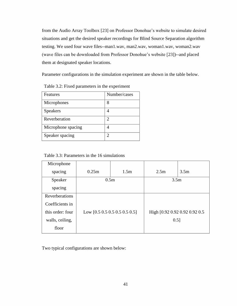
41

from the Audio Array Toolbox [23] on Professor Donohue’s website to simulate desired

situations and get the desired speaker recordings for Blind Source Separation algorithm

testing. We used four wave files--man1.wav, man2.wav, woman1.wav, woman2.wav

(wave files can be downloaded from Professor Donohue’s website [23])--and placed

them at designated speaker locations.

Parameter configurations in the simulation experiment are shown in the table below.

Table 3.2: Fixed parameters in the experiment

Features Number/cases

Microphones 8

Speakers 4

Reverberation 2

Microphone spacing 4

Speaker spacing 2

Table 3.3: Parameters in the 16 simulations

Microphone

spacing

0.25m

1.5m

2.5m

3.5m

Speaker

spacing

0.5m 3.5m

Reverberations

Coefficients in

this order: four

walls, ceiling,

floor

Low [0.5 0.5 0.5 0.5 0.5 0.5]

High [0.92 0.92 0.92 0.92 0.5

0.5]

Two typical configurations are shown below:

42

Figure 3.2: Furthest microphone apart is 3.5m; furthest speaker apart is 3.5m

Figure 3.3: Top view of figure 3.2

0

1

2

3

0

1

2

3

0

0.5

1

1.5

2

Z-D

imensio

n in m

ete

rs

Mic position denote by blue Os, and source positions denoted by red Xs

X-Dimension in metersY-Dimension in meters

0 0.5 1 1.5 2 2.5 3 3.50

0.5

1

1.5

2

2.5

3

3.5


X-Dimension in meters

Y-D

imensio

n in m

ete

rs

43

Table 3.4: Speaker locations in meters for furthest speaker apart is 3.5m

Speaker 1 Speaker 2 Speaker 3 Speaker 4

X direction 0.0780 1.2447 2.4113 3.5780

Y direction 3.0000 3.0000 3.0000 3.0000

Z direction 1.5000 1.5000 1.5000 1.5000

Table 3.5: Microphone locations in meters for furthest speaker apart is 3.5m

Mic 1 Mic 2 Mic 3 Mic 4 Mic 5 Mic 6 Mic 7 Mic 8

X

direction

0.0780 0.5780 1.0780 1.5780 2.0780 2.5780 3.0780 3.578

0

Y

direction

0 0 0 0 0 0 0 0

Z

direction

1.5000 1.5000 1.5000 1.5000 1.5000 1.5000 1.5000 1.500

0

Figure 3.4: Furthest microphone apart is 3.5 m, furthest speaker apart is 0.25 m

0

1

2

3

0

1

2

3

0

0.5

1

1.5

2

Z-D

imensio

n in m

ete

rs



44

Figure 3.5: Top view of figure 3.4

Table 3.6: Speaker locations in meters for furthest speaker apart is 0.25 m

Speaker 1 Speaker 2 Speaker 3 Speaker 4

X direction 0.0780 1.2447 2.4113 3.5780

Y direction 3.0000 3.0000 3.0000 3.0000

Z direction 1.5000 1.5000 1.5000 1.5000

Table 3.7: Microphone locations in meters for furthest speaker apart is 0.25 m


X direction 1.7030 1.7387 1.7744 1.8101 1.8459 1.8816 1.9173 1.9530

Y direction 0 0 0 0 0 0 0 0

Z direction 1.5000 1.5000 1.5000 1.5000 1.5000 1.5000 1.5000 1.5000

0 0.5 1 1.5 2 2.5 3 3.50

0.5

1

1.5

2

2.5

3

3.5



Y-D

imensio

n in m

ete

rs

45

After we simulated 16 different microphone recordings, we used the Conv BSS toolbox,

short for convolutive blind source separation toolbox, to process simulated data in order

to study the two goals mentioned in the beginning of this experiment setup.

We passed the simulated microphone data one by one through the Butterworth High-pass

filter with cutoff frequency 200 Hz. Then we pass the filtered wave channels through the

ConvBSS toolbox developed by M. Castella, S. Rhioui, E. Moreau and J.-C. Pesquet[24]

using the deflation method. Important parameters used in convolutive BSS processing are

number of sources we want to extract, deflation stopping criterion, length(order+1) of the

convolutive extracting filter including anti-causal and causal parts, extraction method,

and parameters specific to the chosen extraction method, such as number of sources that

effectively contribute to the mixture, length of the mixing filter, and number of fixed-

point-like iterations.

The number of sources we want to extract are the estimated underlying sources that

contain most of the information. Deflation stopping criterion is the ratio of the power left

on the sensor divided by power on the sensors initially, after a deflation step. In

Convolutive BSS, this and the estimated number of sources we would like to extract act

like a double threshold to help us extract the optimized extraction results as we can.

Extracting filters is vital in helping us reconstruct information of underlying sources. The

causal filter is a real-time filter that only depends on present and past information; anti-

causal filter cannot be implemented in real-time because it depends on present and future

information. Our application doesn’t need to be real-time, so we use a combination of

causal and anti-causal filters hoping for good separation results. Regarding the extraction

method, for now we use quadratic contrast, SVD-based optimization [24].

Parameters associated with this extraction method are: number of main speakers, length

of mixing filter, number of fixed-point like iteration, and gradient step method. We assign

the same number to the length of the mixing filter and extracting filter. Parameter

specifications used in the simulation tests are below:

46

Table 3.8: Values used in ConvBSS separation process

Parameters Value

Number of Sources 4

Stop Threshold of a Deflation Step 1e-2

Length of the Extracting Filter 100

Length of Anti-causal Part of Extracting

Filter

50

Length of Causal Part of Extracting Filter 50

Source Extraction Method 'quadSVD'

No of Sources Effectively Contribute to

Mixtures

4

Gradient Step 'optim'

After subjective comparison by direct listening to the separated underlying sources, we

decided to focus on the two extreme cases mentioned above, out of the sixteen cases, due

to these comparable better separation effects.

The separated four sources in each case are in the corresponding .wav files. The separated

sources are shown in the figures below.

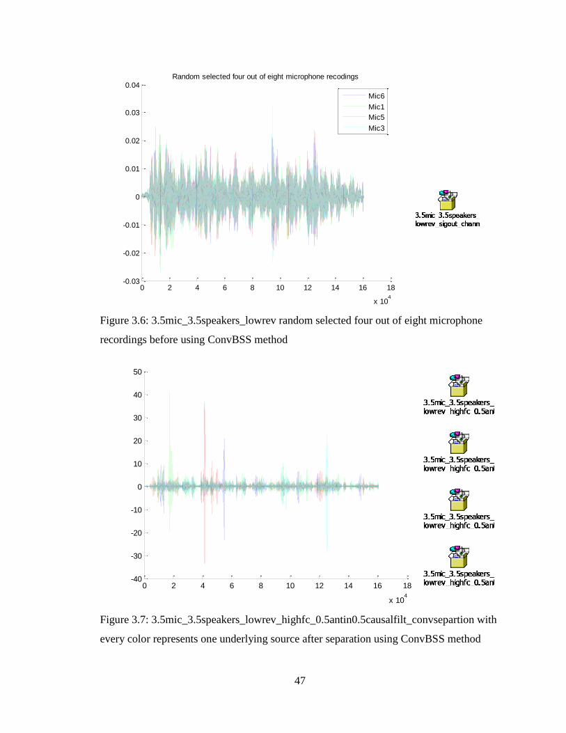
47


recordings before using ConvBSS method

Figure 3.7: 3.5mic_3.5speakers_lowrev_highfc_0.5antin0.5causalfilt_convsepartion with

every color represents one underlying source after separation using ConvBSS method

0 2 4 6 8 10 12 14 16 18

x 104

-0.03

-0.02

-0.01

0

0.01

0.02

0.03

0.04Random selected four out of eight microphone recodings

Mic6

Mic1

Mic5

Mic3

0 2 4 6 8 10 12 14 16 18

x 104

-40

-30

-20

-10

0

10

20

30

40

50

48


recordings before using ConvBSS method

0 2 4 6 8 10 12 14 16 18

x 104

-0.02

-0.015

-0.01

-0.005

0

0.005

0.01

0.015

0.02

0.025Random selected four out of eight microphone recodings

Mic8

Mic3

Mic6

Mic7

0 2 4 6 8 10 12 14 16 18

x 104

-30

-20

-10

0

10

20

30

40

49

Figure 3.9: 0.25mic_3.5speakers_lowrev_highfc_0.5antin0.5causalfilt_convsepartion

with every color represents one underlying source after separation using ConvBSS

method.

When comparing the separated underlying sources for these two cases, we found that

when the microphone apertures are 3.5 meters apart and speaker apertures are 3.5 meters

apart, the estimated underlying sources sound more intelligible.

3.5 Problems Encountered When Using Convolutional BSS Toolbox

When I tried to validate the performance of the Convolutional BSS Toolbox with regards

to the method mentioned in the file Goals of Experiments and Conclusion Derivation

Process_w remarks, I first created an excel file called data.xlsx. Into this excel file, I

manually input all the parameter names and their desired testing values. An example is

shown below in Figure 3.8.

50

Table 3.9 Parameter values to validate the Convolutional BSS Performance

Filename

Nsour

ces

SeuilSt

opAlgo

Lfilt

er

LSubtr

actFiltr

eAC

LSubtrac

tFiltreC

Metho

d

Nsourc

esEffec

tiv

Quadr

atic.L

Quadrat

ic.Nifix

Gradie

ntStep

norspeakerpw4sec_3.5mic_3.5s

peakers_lowrev_sigout.wav 4 0.01 100 50 50

quadS

VD 4 100 10 optim



quadS

VD 4 100 10 optim



quadS

VD 4 100 10 optim



quadS

VD 4 30 10 optim



quadS

VD 4 160 10 optim


peakers_highrev_sigout.wav 4 0.01 100 50 50

quadS

VD 4 100 10 optim



quadS

VD 4 100 10 optim



quadS

VD 4 100 10 optim



quadS

VD 4 30 10 optim



quadS

VD 4 160 10 optim

norspeakerpw4sec_0.25mic_3.5

speakers_lowrev_sigout.wav 4 0.01 100 50 50

quadS

VD 4 100 10 optim



quadS

VD 4 100 10 optim



quadS

VD 4 100 10 optim



quadS

VD 4 30 10 optim



quadS

VD 4 160 10 optim


speakers_highrev_sigout.wav 4 0.01 100 50 50

quadS

VD 4 100 10 optim



quadS

VD 4 100 10 optim



quadS

VD 4 100 10 optim



quadS

VD 4 30 10 optim



quadS

VD 4 160 10 optim

51

Then I wrote a software script in Matab that reads in all the data from the excel file. This

software script is also iterative. For every row of data, it calls the Convolutional BSS

method and computes with the parameter values given using the specific method

designated in the row. When finishing computing, the script will give four separated

underlying sources in .wav format.

Each set of data takes approximately twenty minutes to an hour to get four underlying

sources. After inner and cross comparison of the different separating results by direct

listening we found that some set of the data works better than others.

We picked the four most distinct (in a sense that their timbre are quite unique and easy to

distinguish from a group) sources man1, man2, woman2, and woman3. We selected four

seconds based on the speech density of the wave files of these four wave files so as that

we run ConvBSS algorithm testing, it does not use quite as much time, so we can get a

quick idea of the performance, find the critical parameter, and validate it on the whole

length speech. We then normalized the four sources to the same power level to avoid the

volume interferences of the Convolutional BSS algorithm.

We also ran simulation tests on high reverberation cases. In summary, we ran simulations

with regard to high/low reverberations, different numbers of microphones/speakers

(meaning mixing systems are under/over determined), different microphone/speaker

spacing, different parameter setup for the Convolutive Toolbox, and different filter

length/types of filters (causal/anti-causual). Two typical cases are shown in Figures 3.2

through 3.9. Some of the parameter variation is shown in Table 3.8. Figure 3.2 is a

layout of the best case we have through our experiments. Figure 3.3 is the top view of the

layout. Even in the best case, we do not hear much performance improvement. As far as

all the experiments we have tried, Convolutive BSS failed to show much improvement in

source separation such as difference level of reverberation, different geometry

microphone and speaker layout, different number of microphones, different filter

length/types, etc. Later on, we found that Convolutive BSS has stability issues as well.

The abnormal spikes in Figures 3.7 and 3.9 show stability issues. Later on, we conducted

stability tests on different kinds of algorithms in the Convolutive Toolbox

52

(Toolbox_2.0.3); very rarely can one algorithm in Toolbox_2.0.3 make it. This test shows

stability issues in Toolbox_2.0.3.

From the convolutive algorithm interpretation, it seems that theoretically the Convolutive

BSS should work well dealing with real world recordings and real world recording are

most often convolutive.. However, the toolbox requires many parameters to be set and

often has stability issues as well as minute performance improvement.

53

Chapter 4: Channel Aligned Fast ICA

The FastICA toolbox works well in extracting each source when we have instantaneous

mixture sources. But this toolbox failed to extract any source from mixtures when the

mixture is convolutional. Then we looked into the Matlab toolbox for separation of

convolutive mixtures [25], adjusted it to smoothly interact with audio signals. We also

intensively ran experiments on this toolbox and tried all the separating methods in

Convolutive toolbox. After many experiments as mentioned in the last chapter, we found

that the toolbox is not stable when working with audio signals. As we were trying to fix

this problem by researching this toolbox, we found that researchers just mentioned in

their papers that this toolbox brings in low MSE when sample size was large. Researchers

have not tried working with audio signals/ speech signals using this toolbox and this

toolbox needs quite a bit of development work so as to be more efficient for audio signals.

Other toolboxes that work well with audio signals are Flexible Audio Source Separation

Toolbox (FASST) [26] and BSS Locate (A toolbox for source localization in stereo

convolutive audio mixtures) [27]. FASST toolbox keen methodology is based on

nonnegative matrix factorization (NMF) while BSS Locate toolbox leans more towards

the estimation of Time Differences of Arrival (TDOAs) of sources. FASST does not have

the smooth sound effects on Linear instantaneous mixture after separation while FastICA

toolbox have smooth sound effects, it could not extract all the underlying sources in a

underdetermined situation. BSS Locate Matlab toolbox estimates the Time Differences

of Arrival (TDOAs) of multiple sources in a stereo audio signal recorded by a pair of

omnidirectional microphones. Two different categories of source localization methods

are implemented: angular spectrum-based methods and clustering-based methods. It is

more powerful when combined with other algorithms using TDOAs.

For our cocktail party scenario, we took advantage of the FastICA algorithm (such as

smooth separation effects, fast processing, etc.) and developed a new algorithm, Channel

Aligned Fast ICA (CAICA). Since Convolutive BSS toolbox has many parameters

needed to be setup, it takes time to explore suitable parameters for source separation so it

is not very practical and is time cosuming to use Convoulitve BSS. While FastICA can

54

use just one set of parameters for source separation and it works very well with

instantaneous mixtures but failed to separate Convolutive mixtures, it inspired us to align

all microphone channels to make speaker sound “instantaneous” with respect to all

microphone channels, and then apply FastICA to the aligned mixtures. Source separation

results only have one channel with clear Source of Interest, other channels are all noise.

We can then combine the results with Time Frequency Masking for effective source

separation of from the mixtures. But CAICA brings up a tradeoff because Convolutive

BSS does not need any prior knowledge such as the relative locations of the microphone

and SOI but CAICA does require such information. With the limitation of the weighted

Beamforming such that it could not generate up to the total number of microphones of

meaningful channels. We also prolong the advantages of the algorithm and combine it

with Time Frequency Masking for better sound extracting results (motivation of the new

algorithm).

4.1 CAICA Description

A new algorithm referred to the Channel Aligned FastICA (CAICA) is introduced in the

thesis. This ICA enhancement requires knowledge of the source distance to each

microphone, but does not require knowledge of the noise sources.

Procedures of CAICA are:

1). Calculate delays from SOI to each microphone

2). Apply delays to align SOI signals in each microphone

3). Use Fast ICA for Source Separation of SOI

After applying delays to each microphone channels, from each microphone’s perspective

of view, SOI hits each microphone at approximately the same time.

4.2 Closest Microphone(CM) recordings

Just as its name suggests, Closest Microphone (CM) is the microphone that is closest to

SOI; it performs best amongst microphone arrays. CM recording is used as a reference to

compare with three other algorithms CAICA, WB, CAICA with TFM. Upon comparing,

we can see other algorithms have performance improvements.

55

4.3 Weighted Beamforming (WB):

Beamforming is a signal processing technique that uses spatial information to filter a

target signal of undesired interference [Litva 1996]. Beamforming uses the measured

positions of a target speaker and an array of microphones to calculate optimal methods of

filtering and combining several audio tracks into one with an enhanced SNR.

Weighted Beamforming(WB) weights different microphone channel with regard to its

distance to SOI. A microphone channel that is closer to SOI will have higher weights; a

channel that is farther away from SOI has lower weights.

4.4 Time Frequency Masking (TFM)

Fourier transforms the SOI after processing the Channel (with interferences) and

interference channels in the frequency domain[28,29].

For each time Frequency unit, compare SOI and interferences, if SOI is dominant, keep it;

otherwise put value zero in this unit; that is, mask it out. Hence we have a binary time

frequency mask[28, 29]. We then take the Inverse Fourier Transform to get the processed

audio signals in the time domain.

4.5 CAICA with TF Masking

Furthermore, we combine CAICA with Time Frequency Masking (TFM) yielding even

better SOI extraction even in a harsh environment such as a low SNR environment.

56

Chapter 5: Simulation Experiment

To test the effects of the CAICA and CAICA with TFM, we ran simulations, asked

candidates to evaluate the separation effects and ranked the performance based on direct

listening, and did statistical analysis on the gathered data.

5.1 Simulation Setup

We have eight microphones and four speakers in this set of simulation experiments.

Figure 5.1: Microphones and Speakers 3-D coordinates

0

1

2

3

0

1

2

3

0

0.5

1

1.5

2

Z-D

imensio

n in m

ete

rs



57

Figure 5.2: Microphones and Speakers 3-D coordinates

Table 5.1: Speaker Locations in meters for this setup

X direction 1.0780 1.5780 2.0780 2.5780

Y direction 1.0000 1.0000 1.0000 1.0000

Z direction 1.5000 1.5000 1.5000 1.5000

Table 5.2: Microphone Locations in meters for this setup


X direction 0.0780 0.5780 1.0780 1.5780 2.0780 2.5780 3.0780 3.5780

Y direction 0 0 0 0 0 0 0 0

Z direction 1.5 1.5 1.5 1.5 1.5 1.5 1.5 1.5

From left to right in Figure 5.2, we have microphone 1 to microphone 8.

0 0.5 1 1.5 2 2.5 3 3.50

0.5

1

1.5

2

2.5

3

3.5



Y-D

imensio

n in m

ete

rs

58

5.2 Simulation Procedures

We randomly selected four out of the 12 wave clips, man1, man2, man3, man4, man5,

man6, man7, man8, woman1, woman2, woman3, and woman4 without replication and

put them in the selected order from left to right in four speaker spots. We put 8

microphones in the designated spots. We trimmed randomly selected speaker wave clips

to the same length and passed them through a high pass filter to remove room noise. Then

we normalized each speaker’s power. We randomly selected a speaker location and

treated it as the Speaker of Interest (SOI). We used cocktail function cocktailp(sigin, spos,

mpos, recinfo) to simulate room effects yielding cocktail party data. Here we set

recinfo=0 for no reverberation[23].

Based on room temperature, room humidity and room pressure, we calculated the speed

of sound and we found the distances from SOI to each microphone in meters. We

subtracted every distance from SOI to microphone from the maximum distance and then

divided by speed of sound yielding time durations that each track needs to be delayed so

that SOI hits each microphone at the same time. Then we converted relative time delays

to relative sample delays. We detected the closest microphone channel based on the

minimal delays and labeled it. We padded the number of zeros that are equal to the

relative delays samples in each track and stored data as the microphone aligned data.

We added up all the signals across the 8 microphone channels yielding SOI beamforming

data. Based on the distances from SOI to sensors (microphones); we computed weights

for each sensor. We weighted each channel based on these calculated weights and

summed them up across all eight channels yielding the weighted beam forming (WB)

data.

We processed microphone-aligned data through the FastICA toolbox with optimized

parameters yielding the channel aligned FastICA data. We listened to each channel and

handpicked the processed SOI channel and saved it as the CAICA SOI channel data.

After identifying SOI and interference channels, we processed CAICA data through the

Time Frequency Masking algorithm tfmask.m in the ASA_Toolbox. In the Time

59

Frequency Masking file, for each time window and frequency bin when the SOI value is

larger than each interference, we kept the SOI value, otherwise we masked out (zeroed

out) this frequency bin (zero out this time window) [28, 29]. Then we got the data for the

CAICA with TFM. Figures associated with every algorithm and/or references are shown

from Figure 5.3 through Figure 5.8. Related sound files please seen files linked next to

figures.

Figure 5.3: Normalized SOI (man3)

0 2 4 6 8 10 12 14 16 18-1

-0.8

-0.6

-0.4

-0.2

0

0.2

0.4

0.6

0.8

1Normalized SOI(man3)

Time/s

Sig

nal

60

Figure 5.4: SOI(man3) closest microphone 3

Figure 5.5: SOI(man3) weighted beamforming

0 2 4 6 8 10 12 14 16 18-1

-0.8

-0.6

-0.4

-0.2

0

0.2

0.4

0.6

0.8

1SOI(man3) closest microphone 3

Time/s

Sig

nal

0 2 4 6 8 10 12 14 16 18-1

-0.8

-0.6

-0.4

-0.2

0

0.2

0.4

0.6

0.8

1SOI(man3) weighted beamforming

Time/s

Sig

nal

61

Figure 5.6: SOI (man3) channel adjusted fastICA SOI channel 7

Figure 5.7: SOI(man3)channel adjusted fastICA with time frequency masking

0 2 4 6 8 10 12 14 16 18-1

-0.8

-0.6

-0.4

-0.2

0

0.2

0.4

0.6

0.8

1SOI(man3) channel adjusted fastICA SOI channel 7

Time/s

Sig

nal

0 2 4 6 8 10 12 14 16 18-1

-0.8

-0.6

-0.4

-0.2

0

0.2

0.4

0.6

0.8

1SOI(man3)channel adjusted fastICA with time frequency masking

Time/s

Sig

nal

62

Figure 5.8: All wave forms for comparison

5.3 Experiment Approaches and Descriptions

We then ran the same experiment mentioned above but with lowered SOI volume: 50%,

40%, 35%, 30%, and 25% of the normalized power to find the critical point. When SOI is

100% of the normalized power, it roughly corresponds to -4.7712 dB SNR. 50%, 40%,

35%, 30%, and 25% of the normalized power roughly corresponds to -7.7815dB, -

8.7506dB, -9.3305dB, -10dB, and -10.7918dB SNR. When it comes down to SOI 30%

of normalized power (-10dB SNR), systematic errors occurred such as we cannot identify

the SOI channel in the CAICA data.

100% and 35% of the normalized SOI power (-4.7712 dB and -9.3305dB SNR) were

finalized to compare algorithm performance in the simulation experiments. A total of 16

63

sets of experiments were conducted based on the procedures mentioned above and 8 sets

were with 100% of the normalized SOI power and the other 8 sets were with 35% of the

normalized SOI power.

For each set of experiments, we put five sound tracks in audacity and saved the audacity

file. In each audacity file, the first sound track is always the randomly selected SOI with

the desired power. The rest of the four sound tracks are CM, WB, CAICA SOI channel,

and CAICA with TFM, but not necessarily in the stated order. In fact, the order is

random in order to better judge each algorithm’s performance.

Five laboratory members participated with the goal of nonbiased testing of algorithm

performance. All candidates went over the message in italics first and needed to make

sure they fully understood how the experiment works and the goals before they

proceeded.

Descriptions:

In this experiment, we will listen to and rate 16 sets of files. In each set of files, we have

five sound tracks. The first sound track (reference sound track) is always the Source Of

Insterest (SOI), the rest of the sound tracks are associated with different algorithms not

appearing in the same order in each file.

Question:

Please rank the sound tracks with respect to the degree that SOI speech is extracted from

the other voices with 1 being best and 4 being worst.

Remarks:

Please go back and forth until you are fairly confident with your ranking. Please record

the results in the provided spreadsheet. In the case, when you feel two are the same, give

them an arbitrary ranking.

Candidates will open the experiment file in the audacity with the interface as shown in

Figure 5.9.

64

Figure 5.9: Audacity user interface for one experiment

65

As they went back and forth listening and comparing the quality of the algorithms, they

also recorded the ranking of the sound files in an Excel file for each member. An

example of a set of rankings for a single listener is shown in Table 5.3.

Table 5.3: Test_Laboratory Member A Sound Track Ranking

Sound Track 2 Sound Track 3 Sound Track 4 Sound Track 5

EXP 1 2 1 4 3

EXP 2 2 3 4 1

EXP 3 1 2 3 4

EXP 4 3 4 2 1

EXP 5 1 4 2 3

EXP 6 3 1 2 4

EXP 7 4 2 3 1

EXP 8 2 3 4 1

EXP 9 1 2 4 3

EXP 10 4 1 3 2

EXP 11 3 2 4 1

EXP 12 2 4 3 1

EXP 13 2 1 4 3

EXP 14 2 4 3 1

EXP 15 3 4 1 2

EXP 16 3 1 4 2

Based on the name of each sound track in each experiment in Figure 5.9, Table 5.3 was

converted to Table 5.4, where different algorithm ranking scores are associated with

specific algorithms. Then the score sum and average were calculated for three algorithms

WB, CAICA, CAICA with TFM and one reference CM.

66

Table 5.4: Algorithm Ranking_ Laboratory Member A’s Score

Closest

Microphone

Weighted

Beamforming

Channel Aligned

ICA

Aligned ICA + TF

Masking

exp1 4 2 3 1

exp2 4 2 3 1

exp3 4 3 2 1

exp4 4 3 2 1

exp5 4 3 2 1

exp6 4 3 2 1

exp7 4 3 2 1

exp8 4 3 2 1

exp9 4 2 3 1

exp10 3 4 2 1

exp11 4 3 2 1

exp12 4 2 3 1

exp13 4 2 3 1

exp14 4 2 3 1

exp15 4 2 3 1

exp16 4 3 2 1

Sum 63 42 39 16

Avg 3.9375 2.625 2.4375 1

5.4 Statistical Analysis

Means and standard deviations for each member and for all data sets were calculated and

are shown in the tables below.

67

Table 5.5 Statistical Analysis

Laboratory

Member B

Closest

Microphone

Weighted

Beamforming

Channel aligned

ICA

Aligned ICA +

TFM

Mean 3.9375 2.3125 2.625 1

Standard

Deviations 0.25 0.602079729 0.619139187 0

Laboratory

Member C

Closest

Microphone

Weighted

Beamforming

Channel aligned

ICA

Aligned ICA +

TFM

Mean 4 2.6875 2.3125 1

Standard

Deviations 0 0.478713554 0.478713554 0

Laboratory

Member D

Closest

Microphone

Weighted

Beamforming

Channel aligned

ICA

Aligned ICA +

TFM

Mean 4 2.5 2.5 1

Standard

Deviations 0 0.516397779 0.516397779 0

Laboratory

Member E

Closest

Microphone

Weighted

Beamforming

Channel aligned

ICA

Aligned ICA +

TFM

Mean 4 2.4375 2.5625 1

Standard

Deviations 0 0.512347538 0.512347538 0

Laboratory

Member A

Closest

Microphone

Weighted

Beamforming

Channel aligned

ICA

Aligned ICA +

TFM

Mean 3.9375 2.625 2.4375 1

Standard

Deviations 0.25 0.619139187 0.512347538 0

68

Table 5.5, continued Statistical Analysis

Whole 80 sets

of data

Closest

Microphone

Weighted

Beamforming

Channel aligned

ICA

Aligned ICA +

TFM

Mean 3.975 2.5125 2.4875 1

Standard

Deviations

0.15711 0.5510347 0.527563062 0

5.5 Conclusions

Summarizing all the experiments conducted by all candidates, as well as calculating the

mean and standard deviations mean score for CAICA with TFM is 1; the mean score for

CAICA is 2.4875; the mean score for WB is 2.5125; and the mean score for CM is 3.975.

Standard deviations for each algorithm and reference are 0, 0.53, 0.55, and 0.16

respectively. The mean score for the whole set of experiments shows that CAICA with

TFM performs best in the sense of the degree that SOI speech is extracted from other

voices. CAICA and WB perform next and their performance is about the same, and CM

worst.

Due to the high standard deviations for WB and CAICA and minimum mean value

difference between WB and CAICA, we cannot conclude which one, WB or CAICA,

performs better and these two algorithms perform about the same in source separation.

Since beamforming is a mature technique that has already been deployed to modern

electronic devices, such as cell phones, tablets, etc., even if CAICA performs the same in

source separation, it is already very impressive. The mean and standard deviation values

also show that WB, CAICA, CAICA with TFM improves the performance of the SOI

extraction for sure. Low or 0 standard deviations for all the experiments better support

the conclusion drawn based on mean score.

69

Chapter 6: Algorithm Validation

We have a reference Closest Microphone (CM) for subjective listening comparisons, and

we introduced three algorithms, Weighted Beam forming (WBF), Channel Aligned

FastICA(CAICA) and Channel Aligned FastICA with Time Frequency

Masking(CAICATFM) algorithms in the last chapter and showed their simulation results.

We put emphasis on the performance of the new algorithm (CAICA) and how the new

algorithm performs when combined with TF masking. In this chapter, we are going to

show experimental recording results to validate algorithm performance. One experiment

environment setting for experimental recordings is shown in Figures 6.1 through 6.3.

Figures are from Dr. Donohue Website

http://www.engr.uky.edu/~donohue/audio/Examples/Examples.html

Figure 6.1: Cage side with Linear Microphone array, a couple of speakers, and absorptive

acoustic treatment

70

Figure 6.2: Cage with Speakers side view

Figure 6.3: Cage with Speakers back view

71

6.1 Experiments Setup

We realized a cocktail party scenario in our Audio Systems Laboratory in University of

Kentucky.

We used the data from the Cocktail party recording with distributed microphones (one

speaker of interest embedded in 6 simultaneous speakers). Data can be downloaded from

the link http://www.engr.uky.edu/~donohue/audio/Data/audioexpdata.htm. Specifically,

we used the Microphone Ceiling Regular Hexagonal Grid in this validation experiment.

In this experiment, we have 16 microphones and 1 SOI. Hardware and software

parameters are shown below in Table 6.1.

Table 6.1 Experiment Settings

RT60 Time 0.232 s

Size of Space for

speakers and

microphones

3.6x3.6x2.2

Sampling

Frequency

22050 Hz

Microphones 16 Behringer ECM8000 measurement microphones,

condenser type, Omni direction, Frequency response,

15Hz to 20KHz [30].

Amplifiers M-Audio AudioBuddy Dual Microphone Preamp with

Phantom Power and Direct Box, frequency response:

5Hz-50 KHz[31]

Sound Card Two 8-Channel Delta 1010 by M-Audio

Acoustic Foam

Panels

Auralex MAX-WALL, noise reduction coefficient

1.05[32]

A/D conveter M-Audio Delta 1010 Digital recording system, frequency

response: 20Hz – 22KHz, 8X8 analog I/O[33]

Software Jack audio connection kit 0.3.2, Ubuntu studio 8.04[34]

http://www.engr.uky.edu/~donohue/audio/Data/audioexpdata.htm

72

For these results presented here, we used SOI 5 and background cocktail party noise 3.

The cocktail party noise is a 16 channel recording from 6 talking people. SOI is not

presented in the party noise. 16 microphones are installed on the ceiling shown in blue

circles with coordinates described in Table 6.3. Table 6.2 shows the mean speaker

location. Speaker mean location is also marked as red cross in Figure 6.4. Figure 6.4

shows microphone and mean speaker 3-D locations. Figure 6.5 is the top view of the

microphone and mean speaker location. We can see that microphone locations are like

the Ceiling Regular Hexagonal Grid. We superimposed SOI and party noise recordings

with different SNR values and tested the four algorithms mentioned above. We tested on

three scenarios: SNR=2 dB, SNR = 0 dB, SNR = -10 dB. The 6 interferences are not

marked in the microphone and speaker layout since their locations do not matter to our

program and they were used as noise.

Figure 6.4: 3-D View of the microphone Locations and mean Speaker Location

0

1

2

3

4

0

1

2

3

40

0.5

1

1.5

2

2.5

Mete

rs Z

Mic Positions (Blue o), Source Mean Position (red x)

Meters XMeters Y

73

Figure 6.5: Labeled 16 Microphones and Speaker of Interest Mean Location Top view

Table 6.2: Speaker of Interest (SOI) Mean Coordinates in Meters

SOI

X direction 1.741

Y direction 0.2101

Z direction 1.602

Table 6.3: Microphone Coordinates in meters

M 1 M 2 M 3 M 4 M 5 M 6 M 7 M 8

X direction 3 2 1 0 3.5 2.5 1.5 0.5

Y direction 0 0 0 0 1 1 1 1

Z direction 2 2 2 2 2 2 2 2

M 9 M 10 M 11 M 12 M 13 M 14 M 15 M 16

X direction 3 2 1 0 3.5 2.5 1.5 0.5

Y direction 2 2 2 2 3 3 3 03

Z direction 2 2 2 2 2 2 2 2

0 0.5 1 1.5 2 2.5 3 3.5 40

0.5

1

1.5

2

2.5

3

3.5

4

1234

5678

9101112

13141516

Meters X

Mete

rs Y

Mic Positions (Blue o), Source Mean Position (red x)

74

6.2 Processing Procedures

After we read in the 16 channel source data and 16 channel party noise data, we adjusted

the source and party noise volume with the desired SNR value and added them together

as the cocktail party scene. Now we have 16-channel microphone recordings. We applied

a high pass filter to the microphone recordings to remove room noise. We detected the

closest microphone with respect to the speaker, in this case Microphone 2. We saved data

from the closest microphone channel into a wave file. Hence we got data for the Closest

Microphone (CM) algorithm. We beam-formed on the SOI and applied the adjusted

coefficients to each channel yielding the data for the Weighted Beam Forming (WBF)

algorithm. We then calculated distances from the speaker’s mean location to all 16

microphones and converted these distances to samples and then aligned microphone

recordings base on these samples. Now all microphone channels are aligned with respect

to how quickly the SOI reaches each microphone at the same time instance. Then we

applied FastICA with optimized parameters to the aligned microphone channels yielding

the 16-channel data for the Channel Aligned FastICA algorithm (CAICA). Then we

handpicked the channel with the clearest SOI from the 16-channel CAICA data, marked

the channel number and saved it as SOI CAICA. We then input 16-channel CAICA to the

Time-Frequency Masking. The marked channel is the SOI and other channels are

interferences. Then we got the processed data and saved it as the data for the combined

CAICATFM algorithm.

We compared processed sound clips for four algorithms: CM, WBF, CAICA, and

combined CAICATFM. We validated the algorithm performance by directly listening

and by observing the envelopes of the SOI signals from different algorithms. The

extracted SOI results are shown in Figures 6.6 through 6.34.

Experiment 1: SNR =2 dB

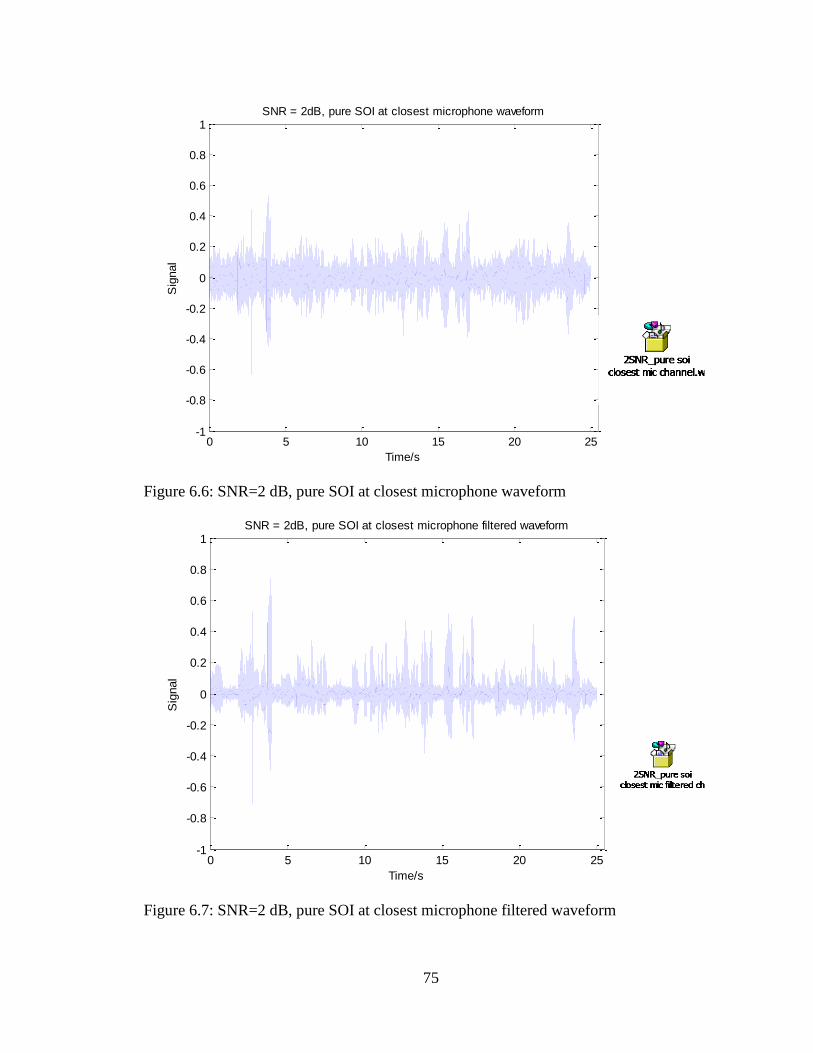
75

Figure 6.6: SNR=2 dB, pure SOI at closest microphone waveform

Figure 6.7: SNR=2 dB, pure SOI at closest microphone filtered waveform

0 5 10 15 20 25-1

-0.8

-0.6

-0.4

-0.2

0

0.2

0.4

0.6

0.8

1SNR = 2dB, pure SOI at closest microphone waveform

Time/s

Sig

nal

0 5 10 15 20 25-1

-0.8

-0.6

-0.4

-0.2

0

0.2

0.4

0.6

0.8

1SNR = 2dB, pure SOI at closest microphone filtered waveform

Time/s

Sig

nal

76

Figure 6.8: SNR=2 dB, cocktail party at closest microphone waveform

Figure 6.9: SNR=2 dB, cocktail party weighted beam forming waveform

0 5 10 15 20 25-1

-0.8

-0.6

-0.4

-0.2

0

0.2

0.4

0.6

0.8

1SNR = 2dB, cocktail party at closest microphone

Time/s

Sig

nal

0 5 10 15 20 25-1

-0.8

-0.6

-0.4

-0.2

0

0.2

0.4

0.6

0.8

1SNR = 2dB, cocktail party weighted beam forming

Time/s

Sig

nal

77


Figure 6.11: SNR = 2 dB, cocktail party channel adjusted fastICA with 16 channel TFM

waveform

0 5 10 15 20 25-1

-0.8

-0.6

-0.4

-0.2

0

0.2

0.4

0.6

0.8

1SNR = 2dB, cocktail party channel adjusted fastICA SOI channel

Time/s

Sig

nal

0 5 10 15 20 25-1

-0.8

-0.6

-0.4

-0.2

0

0.2

0.4

0.6

0.8

1SNR = 2dB, cocktail party channel adjusted fastICA with 16 channel time frequency masking

Time/s

Sig

nal

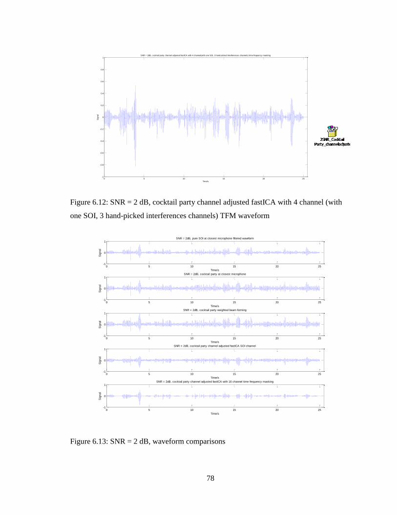
78


one SOI, 3 hand-picked interferences channels) TFM waveform

Figure 6.13: SNR = 2 dB, waveform comparisons

0 5 10 15 20 25-1

-0.8

-0.6

-0.4

-0.2

0

0.2

0.4

0.6

0.8

1SNR = 2dB, cocktail party channel adjusted fastICA with 4 channel(with one SOI, 3 hand-picked interferences channels) time frequency masking

Time/s

Sig

nal

0 5 10 15 20 25-1

0


Time/s

Sig

nal

0 5 10 15 20 25-1

0


Time/s

Sig

nal

0 5 10 15 20 25-1

0


Time/s

Sig

nal

0 5 10 15 20 25-1

0


Time/s

Sig

nal

0 5 10 15 20 25-1

0


Time/s

Sig

nal

79

Figure 6.14: SNR = 2 dB, filtered pure SOI, channel adjusted fastICA with16-channel

time frequency masking, channel adjusted fastICA with4-channel time frequency

masking waveform comparisons

Experiment 2: SNR =0 dB

0 5 10 15 20 25-1

-0.5

0

0.5


Time/s

Sig

nal

0 5 10 15 20 25-1

-0.5

0

0.5


Time/s

Sig

nal

0 5 10 15 20 25-1

-0.5

0

0.5


Time/s

Sig

nal

80

Figure 6.15: SNR=0 dB, pure SOI at closest microphone waveform

Figure 6.16: SNR=0 dB, pure SOI at closest microphone filtered waveform

0 5 10 15 20 25-1

-0.8

-0.6

-0.4

-0.2

0

0.2

0.4

0.6

0.8

1SNR = 0dB, pure SOI at closest microphone waveform

Time/s

Sig

nal

0 5 10 15 20 25-1

-0.8

-0.6

-0.4

-0.2

0

0.2

0.4

0.6

0.8


Time/s

Sig

nal

81

Figure 6.17: SNR=0 dB, cocktail party at closest microphone waveform

Figure 6.18: SNR=0 dB, cocktail party weighted beam forming waveform

0 5 10 15 20 25-1

-0.8

-0.6

-0.4

-0.2

0

0.2

0.4

0.6

0.8


Time/s

Sig

nal

0 5 10 15 20 25-1

-0.8

-0.6

-0.4

-0.2

0

0.2

0.4

0.6

0.8


Time/s

Sig

nal

82


Figure 6.20: SNR = 0 dB, cocktail party channel adjusted fastICA with 16 channel time

frequency masking waveform

0 5 10 15 20 25-1

-0.8

-0.6

-0.4

-0.2

0

0.2

0.4

0.6

0.8


Time/s

Sig

nal

0 5 10 15 20 25-1

-0.8

-0.6

-0.4

-0.2

0

0.2

0.4

0.6

0.8


Time/s

Sig

nal

83


one SOI, 3 hand-picked interferences channels) time frequency masking waveform

Figure 6.22: SNR = 0 dB, waveform comparisons

0 5 10 15 20 25-1

-0.8

-0.6

-0.4

-0.2

0

0.2

0.4

0.6

0.8


Time/s

Sig

nal

0 5 10 15 20 25-1

0


Time/s

Sig

nal

0 5 10 15 20 25-1

0


Time/s

Sig

nal

0 5 10 15 20 25-1

0


Time/s

Sig

nal

0 5 10 15 20 25-1

0


Time/s

Sig

nal

0 5 10 15 20 25-1

0


Time/s

Sig

nal

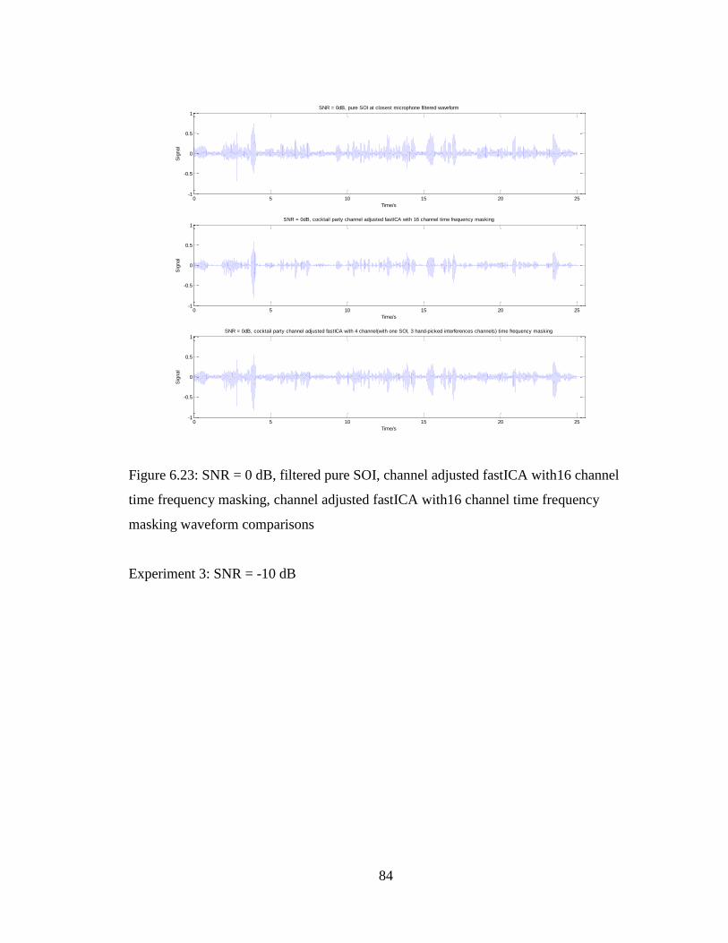
84

Figure 6.23: SNR = 0 dB, filtered pure SOI, channel adjusted fastICA with16 channel

time frequency masking, channel adjusted fastICA with16 channel time frequency

masking waveform comparisons

Experiment 3: SNR = -10 dB

0 5 10 15 20 25-1

-0.5

0

0.5


Time/s

Sig

nal

0 5 10 15 20 25-1

-0.5

0

0.5


Time/s

Sig

nal

0 5 10 15 20 25-1

-0.5

0

0.5


Time/s

Sig

nal

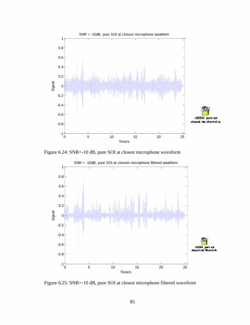
85

Figure 6.24: SNR=-10 dB, pure SOI at closest microphone waveform

Figure 6.25: SNR=-10 dB, pure SOI at closest microphone filtered waveform

0 5 10 15 20 25-1

-0.8

-0.6

-0.4

-0.2

0

0.2

0.4

0.6

0.8

1SNR = -10dB, pure SOI at closest microphone waveform

Time/s

Sig

nal

0 5 10 15 20 25-1

-0.8

-0.6

-0.4

-0.2

0

0.2

0.4

0.6

0.8

1SNR = -10dB, pure SOI at closest microphone filtered waveform

Time/s

Sig

nal

86

Figure 6.26: SNR=-10 dB, cocktail party at closest microphone waveform

Figure 6.27: SNR=-10 dB, cocktail party weighted beam forming waveform

0 5 10 15 20 25-1

-0.8

-0.6

-0.4

-0.2

0

0.2

0.4

0.6

0.8

1SNR = -10dB, cocktail party at closest microphone

Time/s

Sig

nal

0 5 10 15 20 25-1

-0.8

-0.6

-0.4

-0.2

0

0.2

0.4

0.6

0.8

1SNR = -10dB, cocktail party weighted beam forming

Time/s

Sig

nal

87

Figure 6.28: SNR=-10 dB, cocktail party channel adjusted fastICA SOI channel

waveform

Figure 6.29: SNR = -10 dB, cocktail party channel adjusted fastICA with 16 channel time

frequency masking waveform

0 5 10 15 20 25-1

-0.8

-0.6

-0.4

-0.2

0

0.2

0.4

0.6

0.8

1SNR = -10dB, cocktail party channel adjusted fastICA SOI channel

Time/s

Sig

nal

0 5 10 15 20 25-1

-0.8

-0.6

-0.4

-0.2

0

0.2

0.4

0.6

0.8

1SNR = -10dB, cocktail party channel adjusted fastICA with 16 channel time frequency masking

Time/s

Sig

nal

88





0 5 10 15 20 25-1

-0.8

-0.6

-0.4

-0.2

0

0.2

0.4

0.6

0.8

1SNR = -10dB, cocktail party channel adjusted fastICA with 4 channel(with one SOI, 3 hand-picked interferences channels) time frequency masking

Time/s

Sig

nal

0 5 10 15 20 25-1

-0.8

-0.6

-0.4

-0.2

0

0.2

0.4

0.6

0.8


Time/s

Sig

nal

89



Figure 6.33: SNR = -10 dB, waveform comparisons

0 5 10 15 20 25-1

-0.8

-0.6

-0.4

-0.2

0

0.2

0.4

0.6

0.8


Time/s

Sig

nal

0 5 10 15 20 25-1

0


Time/s

Sig

nal

0 5 10 15 20 25-1

0

1SNR = -10dB, cocktail party at closest microphone

Time/s

Sig

nal

0 5 10 15 20 25-1

0

1SNR = -10dB, cocktail party weighted beam forming

Time/s

Sig

nal

0 5 10 15 20 25-1

0

1SNR = -10dB, cocktail party channel adjusted fastICA SOI channel

Time/s

Sig

nal

0 5 10 15 20 25-1

0


Time/s

Sig

nal

90

Figure 6.34: SNR = -10 dB, filtered pure SOI, channel adjusted fastICA with16-channel,

4-channel, 6-channel, 8-channel time frequency masking waveform comparisons

6.3 Results, Comments and Remarks

The pure SOI closest microphone filtered channel is passed through a high-pass filter to

remove room noise. It differs very minutely from the pure SOI closest microphone

channel by direct listening and it shows a cleaner envelope with important characteristics

more prominent. This minute difference we heard is room noise. The pure SOI closest

microphone filtered channel has lower noise in the sound clip than the pure SOI closest

microphone channel, but either way the SOI is very clear. We heard interference from

party noise meaning other people’s speech in the cocktail party closest microphone sound

clip. Party noise was also in the cocktail party weighted beamforming as well as the

cocktail party channel adjusted fastICA SOI channel. But the party noise was weaker in

WB and CAICA. In the meantime, SOI is most intelligible in CAICA with TFM, more

0 5 10 15 20 25-1

0


Time/s

Sig

nal

0 5 10 15 20 25-1

0


Time/s

Sig

nal

0 5 10 15 20 25-1

0


Time/s

Sig

nal

0 5 10 15 20 25-1

0


Time/s

Sig

nal

0 5 10 15 20 25-1

0


Time/s

Sig

nal

91

intelligible in WB and CAICA, and not very intelligible in the cocktail party closest

microphone channel. I heard no interference, just the SOI, in the resulting CAICATFM.

When SNR values dropped, the SOI was buried in the party noise (6 other speakers’

speech) in CM, WB, CAICA and started to immerge in 16-channel CAICATFM. CM

degraded most. WB and CAICA degraded about the same, 16-channel CAICATFM only

degrades slightly. Speech intelligibility is the degree that the listener can correctly

understand the speech [23].

SOI was intelligible when SNR=2 dB in all cases, but CAICATFM was more intelligible

than CAICA and WB and CM last. When SNR dropped, regarding the intelligibility,

algorithms performed in the same order as mentioned above, but the CM became not very

intelligible (a lot of noise in the sound clip and one could not tell what SOI is talking

about very well), WB and CAICA were still pretty intelligible (noise was more

prominent, but one can still tell what SOI is talking about if one listens closely). In the

meantime, CAICA was still intelligible with very little noise interference.

For each SNR value, by observing the envelopes of the sound tracks and comparing them

with the SOI in three different SNR experiments, as well as by directly listening, we find

that CAICA and TFM combined algorithm performs the best, CAICA and WB perform

about the same and perform second best, and closest microphone performs worst.

Specifically, the CAICATFM combined algorithm performs better is in the sense of less

interfering sound and prominent SOI content. This is consistent with the visual

observations of the envelope of SOI of the algorithm in that it better follows the envelope

of the filtered pure SOI.

When the SNR value is high, i.e. SNR=2 dB, the closest microphone has a fairly high SII,

meaning the SOI is quite clear. When SNR is low, i.e. SNR =-10dB, we cannot very

easily tell the SOI from the closest microphone recording anymore and then the

advantages of the CAICA and combined CAICATFM, WB algorithm become more

prominent.

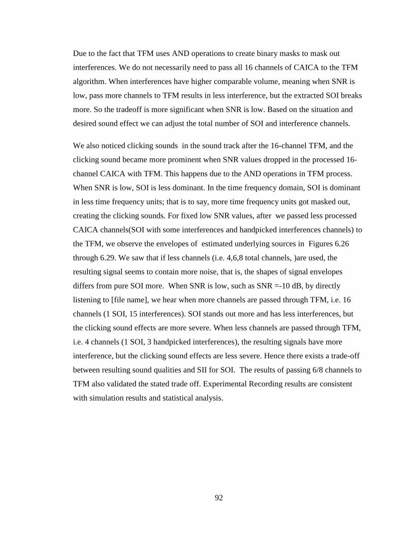
92

Due to the fact that TFM uses AND operations to create binary masks to mask out

interferences. We do not necessarily need to pass all 16 channels of CAICA to the TFM

algorithm. When interferences have higher comparable volume, meaning when SNR is

low, pass more channels to TFM results in less interference, but the extracted SOI breaks

more. So the tradeoff is more significant when SNR is low. Based on the situation and

desired sound effect we can adjust the total number of SOI and interference channels.

We also noticed clicking sounds in the sound track after the 16-channel TFM, and the

clicking sound became more prominent when SNR values dropped in the processed 16-

channel CAICA with TFM. This happens due to the AND operations in TFM process.

When SNR is low, SOI is less dominant. In the time frequency domain, SOI is dominant

in less time frequency units; that is to say, more time frequency units got masked out,

creating the clicking sounds. For fixed low SNR values, after we passed less processed

CAICA channels(SOI with some interferences and handpicked interferences channels) to

the TFM, we observe the envelopes of estimated underlying sources in Figures 6.26

through 6.29. We saw that if less channels (i.e. 4,6,8 total channels, )are used, the

resulting signal seems to contain more noise, that is, the shapes of signal envelopes

differs from pure SOI more. When SNR is low, such as SNR =-10 dB, by directly

listening to [file name], we hear when more channels are passed through TFM, i.e. 16

channels (1 SOI, 15 interferences). SOI stands out more and has less interferences, but

the clicking sound effects are more severe. When less channels are passed through TFM,

i.e. 4 channels (1 SOI, 3 handpicked interferences), the resulting signals have more

interference, but the clicking sound effects are less severe. Hence there exists a trade-off

between resulting sound qualities and SII for SOI. The results of passing 6/8 channels to

TFM also validated the stated trade off. Experimental Recording results are consistent

with simulation results and statistical analysis.

93

Chapter 7: Final Conclusions and Future Work

7.1 Conclusions

The goal of this thesis was to explore the Blind Source Separation in Immersive Audio

Environments and specifically Independent Component Analysis in Cocktail Party

Scenario. After researching and testing on feasibility of a variety of algorithms, FastICA

toolbox stands out with regard to fast convergence, smooth separated audio sound tracks,

does not need feature training and so on. It also works well in separating instantaneous

mixtures, but it comes with limitations as do all algorithms. To estimate all the

underlying sources, FastICA needs the system to be over-determined (mixture channels

are greater and equal to source channels). The estimated underlying source channel is not

fixed after each FastICA algorithm run. To cope with it, we can use auto-correlation to

find the matching pairs.

When we applied the cocktail party recordings, FastICA toolbox failed to recover

sources.Cocktail party recordings are always convolutive and real world recordings are

convolutive as well.The Convolutive BSS algorithm theoretically should be powerful in

source separation for real world recording, but the associated Convolutive BSS toolbox

requires setting up many parameters and often has stability issues. And this toolbox

improves minute source intelligence after we applied the toolbox to the simulated

microphone mixtures.

Then we analyzed factors that make FastICA break in real world settings and after trial

and error, we came up with the Channel Aligned FastICA (CAICA) that enhanced the

FastICA source separation when mixtures are convolutive. In addition, we combined

CAICA with TFM for an even better source separation and recovered source

interligibility. Simulation experimental recording validation are conducted to compare

existing and mature audio source separation Weighted Beam-forming (WB),CAICA and

CAICA with TFM. These experiments as well as statistical analysis prove that CAICA

with TFM works great in source separation as well as high intelligibility recovery and

94

this algorithm is very powerful. CAICA performs slightly better than WB, which is

impressive. All three algorithms perform better than closest microphone (CM), meaning

there are improvements in source separation.

7.2 Future Work

Potentially we can observe the silence period from each algorithm and compare the silent

period with the source of interest to calculate the performance metric. We can also take

down the masker scale level in the TFM so as to pass a few interference channels, but to

achieve the desired TFM effects more interference channels are needed.

Design a graphic user interface (GUI) so as users can play with all the source separation

method mentioned. In that way, users can get more involved in the underlying source

separation process. Furthermore, we can break the whole process into layers, cocktail

party simulation layer, filtering processing layer, and source separation layers. In the

source separation layer, users can choose WB, CAICA, and CAICA with TFM and listen

to each separation effect. All these layers can be wrapped up in one panel. Users can

select, mix or match these three main parts for the desired effects. For example, users can

import their data and then process their data through the filtering processing layer and

source separation layer to listen to different algorithms’ sound effects. Researchers can

also use the layer they desire to conveniently test their algorithms.

A median filter or adaptive filters can potentially be added to smooth out the time domain

audio signals obtained after TFM so as to reduce the clicking sounds for smoother sound

quality. We can potentially fix the ConvBSS toolbox so it works with Audio signals.

Explore the other mentioned algorithms and see how well each algorithm performs

regarding source separation. Researchers can also explore what the separation

performance will be like when combining a few of these separation algorithms. We can

also develop an automated selected tool to select a more proper algorithm for the specific

scenarios. Scenarios can be categorized to number of microphones, number of speakers,

systems is over-determined or underdetermined, number of sources we would like to

95

extract from the signal mixtures, relative locations of microphones and/ or speakers, and

how microphone / speakers are grouped.

Researchers can also explore how we can deploy these techniques modern electronic

devices such as cellphones and tablets as well as explore how these techniques are

applied to surveillance. Researchers can also see how we can download these algorithms

to embedded systems such as Digital Signal Processors for commercial usages.

96

References

[1] Hyvärinen, Aapo, and Erkki Oja. "Independent component analysis: algorithms and

applications." Neural networks 13.4 (2000): 411-430.

[2] Lee, Te-Won. Independent component analysis. Springer US, 1998.

[3] Godara, Lal Chand, ed. Handbook of antennas in wireless communications. Vol. 4.

CRC press, 2010.

[4] S. Makino, T.-W. Lee, H. Sawada (Eds.), Blind Speech Separation, Springer,

Dordrecht, theNetherlands, 2007.

[5] M.E. Lockwood, D.L. Jones, R.C. Bilger, C.R. Lansing, W.D. O’Brien, B.C. Wheeler,

A.S. Feng, Performance of time- and frequency-domain binaural beamformers based

on recorded signals from real rooms, Journal of the Acoustical Society of America

115 (2004) 379–391.

[6] Aapo Hyvärinen, Juha Karhunen, Erkki Oja, Independent Component Analysis,

Volume 26 of Adaptive and Learning Systems for Signal Processing,

Communications and Control Series , Wiley, 2001

[7] Bishop, Christopher M., Markus Svensén, and Christopher KI Williams. "GTM: The

generative topographic mapping." Neural computation 10.1 (1998): 215-234.

[8] Neal, Radford M. Bayesian learning for neural networks. Diss. University of Toronto,

1995.

[9] Barber, David, and Christopher M. Bishop. "Ensemble learning in Bayesian neural

networks." NATO ASI SERIES F COMPUTER AND SYSTEMS SCIENCES 168

(1998): 215-238.

[10] Tong, L., et al. "AMUSE: a new blind identification algorithm." Circuits and

Systems, 1990., IEEE International Symposium on. IEEE, 1990.

[11] Ozerov, A.; Philippe, P.; Gribonval, R.; Bimbot, F., "One microphone singing voice

separation using source-adapted models," Applications of Signal Processing to

Audio and Acoustics, 2005. IEEE Workshop on , vol., no., pp.90,93, 16-19 Oct. 2005.

URL: http://ieeexplore.ieee.org/stamp/stamp.jsp?tp=&arnumber=1540176&isnumber=32

894

[12] A. P. Dempster, N. M. Laird, and D. B. Rubin., Maximum likelihood from

incomplete data via the EM algorithm, Journal of the Royal Statistical Society, 1977.

[13] Douglas, S.C.; Gupta, M.; Sawada, H.; Makino, S., "Spatio–Temporal FastICA

Algorithms for the Blind Separation of Convolutive Mixtures," Audio, Speech, and

Language Processing, IEEE Transactions on , vol.15, no.5, pp.1511,1520, July 2007,

URL: http://ieeexplore.ieee.org/stamp/stamp.jsp?tp=&arnumber=4244514&isnumber=42

44504

[14] J. Thomas, Y. Deville, and S. Hosseini, “Time domain fast fixed-point algorithms

for convolutive ICA,” IEEE Signal Process. Lett., vol. 13, no. 4, pp. 228–230, Apr.

2006.

[15] Málek, J., Koldovský, Z., Tichavský, P.: Adaptive time-domain blind separation of

speech signals. In: Vigneron, V. (ed.) LVA/ICA 2010. LNCS, vol. 6365, pp. 9–16.

Springer, Heidelberg (2010)

URL:http://link.springer.com/chapter/10.1007/978-3-642-15995-4_2

[16] Koldovsky, Z., Tichavsky, P.: Time-domain blind audio source separation using

http://www.google.com/search?tbo=p&tbm=bks&q=inauthor:%22Aapo+Hyv%C3%A4rinen%22&source=gbs_metadata_r&cad=5

http://www.google.com/search?tbo=p&tbm=bks&q=inauthor:%22Juha+Karhunen%22&source=gbs_metadata_r&cad=5

http://www.google.com/search?tbo=p&tbm=bks&q=inauthor:%22Erkki+Oja%22&source=gbs_metadata_r&cad=5

http://www.google.com/search?tbo=p&tbm=bks&q=bibliogroup:%22Adaptive+and+Learning+Systems+for+Signal+Processing,+Communications+and+Control+Series%22&source=gbs_metadata_r&cad=5

http://www.google.com/search?tbo=p&tbm=bks&q=bibliogroup:%22Adaptive+and+Learning+Systems+for+Signal+Processing,+Communications+and+Control+Series%22&source=gbs_metadata_r&cad=5

http://ieeexplore.ieee.org/stamp/stamp.jsp?tp=&arnumber=1540176&isnumber=32894




http://link.springer.com/chapter/10.1007/978-3-642-15995-4_2

97

advanced component clustering and reconstruction. In: HSCMA 2008, Trento, Italy,

pp. 216–219 (2008)

[17] Tichavsky, P., Yeredor, A.: Fast Approximate Joint Diagonalization Incorporating

Weight Matrices. IEEE Transactions of Signal Processing 57(3), 878–891 (2009)

[18] Araki, S., Sawada, H., Mukai, R., & Makino, S. (2011). DOA estimation for

multiple sparse sources with arbitrarily arranged multiple sensors. Journal of Signal

Processing Systems, 63(3), 265-275.

URL:http://link.springer.com/article/10.1007/s11265-009-0413-9

[19] Vincent, E., Araki, S., Theis, F., Nolte, G., Bofill, P., Sawada, H., ... & Duong, N.Q.

(2012). The signal separation evaluation campaign (2007–2010): Achievements and

remaining challenges. Signal Processing, 92(8), 1928-1936.

URL: http://hal.inria.fr/docs/00/63/09/85/PDF/vincent_SigPro11.pdf

[20] Comon, Pierre, and Christian Jutten. Handbook of Blind Source Separation:

Independent component analysis and applications. Access Online via Elsevier, 2010.

[21] Douglas, Scott C., and Xiaoan Sun. "Convolutive blind separation of speech

mixtures using the natural gradient." Speech Communication 39.1 (2003): 65-78.

[22] Michael Syskind Pedersen, Jan Larsen, Ulrik Kjems, and Lucas C Parra, A Survey

of Convolutive Blind Source Separation Methods. Multichannel Speech Processing

Handbook (2007): 1065-1084.

[23] K. D. Donohue, “Audio array toolbox”, September 2008.

URL: http://www.engr.uky.edu/~donohue/audio/Arrays/MAToolbox.html

[24] M. Castella, S. Rhioui, E. Morean and J.-C. Pesquet, Quadratic Higher-Order

Criteria for Iterative Blind Separation of a MIMO Convolutive Mixture of Sources.

IEEE Trans. Signal Processing.

[25] http://www-public.int-evry.fr/~castella/toolbox/gettingstarted.php

[26] Ozerov, Alexey, Emmanuel Vincent, and Frédéric Bimbot. "A general flexible

framework for the handling of prior information in audio source separation." Audio,

Speech, and Language Processing, IEEE Transactions on 20.4 (2012): 1118-1133.

[27] C. Blandin, A. Ozerov and E. Vincent Multi-source TDOA estimation in reverberant

audio using angular spectra and clustering, Signal Processing 92, pp. 1950-1960,

2012. http://bass-db.gforge.inria.fr/bss_locate/

[28] Roman, Nicoleta, DeLiang Wang, and Guy J. Brown. "Speech segregation based on

sound localization." Neural Networks, 2001. Proceedings. IJCNN'01. International

Joint Conference on. Vol. 4. IEEE, 2001.

[29] Srinivasan, Soundararajan, Nicoleta Roman, and DeLiang Wang. "Binary and ratio

time-frequency masks for robust speech recognition." Speech Communication 48.11

(2006): 1486-1501.

[30] Behringer©, "Measurement Microphone ECM8000", Specification sheet, Bheringer

Spezielle Studiotechnik GmbH, 2000.

[31] Avid Technology, Inc., Audio Buddy™, 2009.

www.maudio.com/products/en_us/AudioBuddy.html

[32] Auralex Acoustics, Inc., MAX-Wall Acoustic Panels, 2009.

http://www.auralex.com/testdata/

[33] Avid Thecnology, Inc., Delta 1010™ Digital Recording System, 2009.

www.maudio.com/products/en_us/delta1010.html

[34] Paul Davis, Jack Connection Kit, jackaudio.org, 2006.

http://link.springer.com/article/10.1007/s11265-009-0413-9

http://hal.inria.fr/docs/00/63/09/85/PDF/vincent_SigPro11.pdf

http://www.engr.uky.edu/~donohue/audio/Arrays/MAToolbox.html

http://hal.inria.fr/inria-00630994/PDF/blandin_SigPro11.pdf

http://hal.inria.fr/inria-00630994/PDF/blandin_SigPro11.pdf

98

Vita

Yue Zhao was born in Jiangsu, China. She received Bachelor’s of Science in Electrical

Engineering from the University of Kentucky. She was awarded the Elise White Boyd

Graduate Fellowship and PEIK Graduate Full Tuition Scholarship.

Documents

Independent Component Analysis Enhancements for Source