Embed Size (px)
Citation preview

Incremental Development and Cost-basedEvaluation of Software Fault Prediction Models
Yue Jiang
Dissertation submitted to theCollege of Engineering and Mineral Resources
at West Virginia Universityin partial fulfillment of the requirements
for the degree of
Doctor of Philosophyin
Computer and Information Sciences
Dr. Bojan Cukic, Ph.D., Co-ChairDr. Tim Menzies , Ph.D., Co-Chair
Dr. Arun Ross, Ph.D.Dr. Katerina Goseva-Popstojanova, Ph.D.
Dr. James Harner, Ph.D.
Lane Department of Computer Science and Electrical Engineering
Morgantown, West Virginia2009
Keywords: fault-proneness, prediction, requirement, design, software metricsmachine learning, classification
Copyright 2009 Yue Jiang

ABSTRACT
Incremental Development and Cost-based Evaluation of Software Fault PredictionModels
Yue Jiang
It is difficult to build high quality software with limited quality assurance budgets. Software fault predic-tion models can be used to learn fault predictors from software metrics. Fault prediction prior to softwarerelease can guide Verification and Validation (V &V ) activity and allocate scarce resources to moduleswhich are predicted to be fault-prone.
One of the most important goals of fault prediction is to detect fault prone modules as early aspossible in the software development life cycle. Design and code metrics have been successfully usedfor predicting fault-prone modules. In this dissertation, we introduce fault prediction from softwarerequirements. Furthermore, we investigate the advantages of the incremental development of softwarefault prediction models, and we compare the performance of these models as the volume of data and theirlife cycle origin (design, code, or their combination) evolution during project development. We confirmthat increasing the volume of training data improves model performance. And that, models built fromcode metrics typically outperform those built using design metrics only. However, both types of modelsprove to be useful as they can be constructed in different phases of the life cycle. We also demonstratethat models that utilize a combination of design and code level metrics outperform models which useeither one metric set exclusively.
In evaluation of fault prediction models, misclassification cost has been neglected. Using a graphical
measurement, the cost curve, we evaluate software fault prediction models. Cost curves not only allow
software quality engineers to introduce project-specific misclassification costs into model evaluation, but
also allow them to incorporate module-specific misclassification costs into model evaluation. Classifying
a software module as fault-prone implies the application of some verification activities, thus adding to
the development cost. Misclassifying a module as fault free carries the risk of system failure, and is also
associated with cost implications. Our results, through the analysis of more than ten projects from public
repositories, support a recommendation to adopt cost curves as one of the standard methods for software
fault prediction model performance evaluation.

Acknowledgements
I would like to thank my advisor, Dr. Bojan Cukic, for his guidance, advice, and continualencouragement. It is a pleasure to work under his supervision. Without him, this dissertationcould not have come about. I would like to thank my other advisor, Dr. Tim Menzies, for hisguidance, advice, and help in my study, research, and dissertation.
I would also like to thank my other committee members: Dr. Arun Ross, Dr. KaterinaGoseva-Popstojanova, and Dr. James Harner for their help during my studies.
And finally, I thank my family members for their constant support, encouragement, andhelp.
iii

Contents
1 Introduction 1
2 Related Work 5
2.1 Fault Prediction Modeling . . . . . . . . . . . . . . . . . . . . . . . . . . . . 6
2.1.1 Machine Learning . . . . . . . . . . . . . . . . . . . . . . . . . . . . 7
2.2 Different Approaches for Fault Prediction Models . . . . . . . . . . . . . . . . 15
2.2.1 Supervised Learning . . . . . . . . . . . . . . . . . . . . . . . . . . . 16
2.2.2 Unsupervised Learning . . . . . . . . . . . . . . . . . . . . . . . . . . 17
2.3 Metrics Used in Software Fault Prediction Models . . . . . . . . . . . . . . . . 17
2.4 Model Evaluation Techniques . . . . . . . . . . . . . . . . . . . . . . . . . . 20
2.4.1 Methodology for 2-class Classification . . . . . . . . . . . . . . . . . 20
2.4.2 Graphical Evaluation Methods . . . . . . . . . . . . . . . . . . . . . . 23
2.4.3 Statistical Comparisons of Classification Models . . . . . . . . . . . . 28
2.5 MDP Data Sets and Prior Experiments . . . . . . . . . . . . . . . . . . . . . . 30
iv
2.6 Heuristic . . . . . . . . . . . . . . . . . . . . . . . . . . . . . . . . . . . . . . 35
3 Prediction from Requirement Metrics 37
3.1 Static Requirements Features . . . . . . . . . . . . . . . . . . . . . . . . . . . 38
3.2 Experimental Design and Result . . . . . . . . . . . . . . . . . . . . . . . . . 39
3.2.1 Experimental Design . . . . . . . . . . . . . . . . . . . . . . . . . . . 39
3.2.2 Prediction from Requirements Metrics . . . . . . . . . . . . . . . . . . 42
3.2.3 Prediction from Static module metrics . . . . . . . . . . . . . . . . . . 44
3.2.4 Combining Requirement and Module Metrics . . . . . . . . . . . . . . 46
3.3 Discussion . . . . . . . . . . . . . . . . . . . . . . . . . . . . . . . . . . . . . 48
3.4 Summary . . . . . . . . . . . . . . . . . . . . . . . . . . . . . . . . . . . . . 52
4 Incremental Development of Software Fault Prediction Models 54
4.1 Experimental Design . . . . . . . . . . . . . . . . . . . . . . . . . . . . . . . 54
4.1.1 Design of Experiments . . . . . . . . . . . . . . . . . . . . . . . . . . 55
4.2 Experimental Results . . . . . . . . . . . . . . . . . . . . . . . . . . . . . . . 57
4.2.1 Increasing the size of training set . . . . . . . . . . . . . . . . . . . . . 57
4.2.2 Comparison of design, code, and all metrics models . . . . . . . . . . 68
4.2.3 Comparison of models developed using different classifiers . . . . . . . 75
4.3 Discussion . . . . . . . . . . . . . . . . . . . . . . . . . . . . . . . . . . . . . 80
4.4 Summary . . . . . . . . . . . . . . . . . . . . . . . . . . . . . . . . . . . . . 82
v

5 Cost-specific Fault Prediction Models 85
5.1 Cost Models . . . . . . . . . . . . . . . . . . . . . . . . . . . . . . . . . . . . 85
5.1.1 Cost Curve . . . . . . . . . . . . . . . . . . . . . . . . . . . . . . . . 86
5.2 Experimental Design . . . . . . . . . . . . . . . . . . . . . . . . . . . . . . . 93
5.3 Comparison of the “Best” Classifier Against the Trivial Classifier . . . . . . . . 94
5.3.1 Analysis . . . . . . . . . . . . . . . . . . . . . . . . . . . . . . . . . 95
5.4 Comparison of the “Best” and the “Worst” Classifiers . . . . . . . . . . . . . . 100
5.5 Incorporating Module Priority . . . . . . . . . . . . . . . . . . . . . . . . . . 101
5.5.1 Nearest neighbor method . . . . . . . . . . . . . . . . . . . . . . . . . 102
5.5.2 Priority incorporated evaluation . . . . . . . . . . . . . . . . . . . . . 105
5.6 Summary . . . . . . . . . . . . . . . . . . . . . . . . . . . . . . . . . . . . . 110
6 Conclusion and Future Work 113
6.1 Future Works . . . . . . . . . . . . . . . . . . . . . . . . . . . . . . . . . . . 116
vi

List of Tables
2.1 An example of training subset . . . . . . . . . . . . . . . . . . . . . . . . . . 9
2.2 Summarized statistics of the example training subset. . . . . . . . . . . . . . . 10
2.3 Datasets used in this dissertation . . . . . . . . . . . . . . . . . . . . . . . . . 32
2.4 Metrics used. . . . . . . . . . . . . . . . . . . . . . . . . . . . . . . . . . . . 34
3.1 Requirement Metrics. . . . . . . . . . . . . . . . . . . . . . . . . . . . . . . 39
3.2 The result of inner join on CM1 requirement and module metrics. . . . . . . . 41
3.3 The associations between modules and requirements in CM1, JM1 and PC1. . 42
4.1 Median(m) and variance(v) of 10%, 50%, and 90% training subset models fromdesign metrics, measured by AUC . . . . . . . . . . . . . . . . . . . . . . . . 59
4.2 Median(m) and variance(v) for models trained from 10%, 50%, and 90% ofmodules using code metrics, measured by AUC. . . . . . . . . . . . . . . . . 64
4.3 Median(m) and variance(v) of models built from 10%, 50%, and 90% of moduleusing all metrics, measured by AUC . . . . . . . . . . . . . . . . . . . . . . 66
4.4 Median and variance of AUC on design metrics of using 50% data as the train-ing subset . . . . . . . . . . . . . . . . . . . . . . . . . . . . . . . . . . . . . 78
vii

4.5 Median and variance of AUC on code metrics of using 50% data as the trainingsubset . . . . . . . . . . . . . . . . . . . . . . . . . . . . . . . . . . . . . . . 79
4.6 Median and variance of AUC on all metrics of using 50% data as the trainingsubset . . . . . . . . . . . . . . . . . . . . . . . . . . . . . . . . . . . . . . . 80
5.1 Probability cost of interested and significant ranges. . . . . . . . . . . . . . . . 97
5.2 Comparison of the “best” vs. the “worst” performance classifiers. . . . . . . . 100
5.3 Comparison the similarity of three different distance methods. . . . . . . . . . 103
5.4 Priority distribution of five projects. . . . . . . . . . . . . . . . . . . . . . . . 103
5.5 Probability cost of interested and significant ranges of MC1 and KC3. . . . . . 105
5.6 Comparison of the “best” vs. the “worst” performance classifiers on MC1 andKC3. . . . . . . . . . . . . . . . . . . . . . . . . . . . . . . . . . . . . . . . . 105
5.7 Priority ranges and significant differences for five projects. . . . . . . . . . . . 106
5.8 Performance thresholds for three priorities in KC3, PC1, and PC4 high riskprojects. . . . . . . . . . . . . . . . . . . . . . . . . . . . . . . . . . . . . . . 107
5.9 Comparison of Normalized Expected Cost (NEC) with and without module spe-cific priority . . . . . . . . . . . . . . . . . . . . . . . . . . . . . . . . . . . . 110
viii

List of Figures
2.1 A confusion matrix of prediction outcomes. . . . . . . . . . . . . . . . . . . . 21
2.2 ROC analysis. . . . . . . . . . . . . . . . . . . . . . . . . . . . . . . . . . . . 24
2.3 ROC curve (a) and PR curve (b) of models built from PC5 module metrics . . . 25
2.4 Boxplots of PC5 data set . . . . . . . . . . . . . . . . . . . . . . . . . . . . . 27
2.5 An example of Demsar’s significance diagrams. . . . . . . . . . . . . . . . . . 30
2.6 The Friedman test on design metrics models using AUC for performance eval-uation. . . . . . . . . . . . . . . . . . . . . . . . . . . . . . . . . . . . . . . . 31
3.1 An entity-relationship diagram relates project requirements to modules and mod-ules to faults . . . . . . . . . . . . . . . . . . . . . . . . . . . . . . . . . . . . 40
3.2 CM1 r prediction using requirements metrics only. . . . . . . . . . . . . . . . 43
3.3 JM1 r prediction using requirements metrics only. . . . . . . . . . . . . . . . . 44
3.4 PC1 r prediction using requirements metrics only. . . . . . . . . . . . . . . . . 45
3.5 CM1 r using module metrics. . . . . . . . . . . . . . . . . . . . . . . . . . . . 46
3.6 JM1 r using module metrics. . . . . . . . . . . . . . . . . . . . . . . . . . . . 47
3.7 PC1 r using module metrics. . . . . . . . . . . . . . . . . . . . . . . . . . . . 48
ix

3.8 CM1 RM model uses requirements and module metrics. . . . . . . . . . . . . 49
3.9 PC1 RM model uses requirements and module metrics. . . . . . . . . . . . . . 50
3.10 ROC curves for CM1 project. . . . . . . . . . . . . . . . . . . . . . . . . . . . 51
3.11 ROC curves for JM1 project. . . . . . . . . . . . . . . . . . . . . . . . . . . . 51
3.12 ROC curves for PC1 project. . . . . . . . . . . . . . . . . . . . . . . . . . . . 52
4.1 Boxplot diagrams of using 10%, 50%, and 90% data as training subset ondesign metrics, measured by AUC. In x-axis, “1” stands for 10%; “5” standsfor 50%; “9” stands for 90%. . . . . . . . . . . . . . . . . . . . . . . . . . . 61
4.2 The Friedman test on code metrics models evaluated using AUC. . . . . . . . . 62
4.3 Boxplot diagrams of fault prediction models built from 10%, 50%, and 90% ofdata using code metrics, measured by AUC. In x-axis, “1” stands for 10%; “5”stands for 50%; “9” stands for 90%. . . . . . . . . . . . . . . . . . . . . . . . 63
4.4 The Friedman test on all metrics using AUC. . . . . . . . . . . . . . . . . . . 65
4.5 Box-plot diagrams of fault prediction models built from 10%, 50%, and 90% ofdata using all metrics, measured by AUC. In x-axis, “1” stands for 10%; “5”stands for 50%; “9” stands for 90%. . . . . . . . . . . . . . . . . . . . . . . . 67
4.6 Boxplots comparisons of the performance of models built from design(d), code(c),and all(a) metrics using 10% data as training subset. . . . . . . . . . . . . . . 69
4.7 Statistical performance ranks of design, code, and all models built using 10%data for training. . . . . . . . . . . . . . . . . . . . . . . . . . . . . . . . . . . 70
4.8 Boxplots comparison of the performance of all(a), code(c), and design(d) met-rics using 50% of data for training. . . . . . . . . . . . . . . . . . . . . . . . . 73
4.9 Statistical performance ranks of design, code, and all models built using 50%of data for training. . . . . . . . . . . . . . . . . . . . . . . . . . . . . . . . . 74
x

4.10 Comparison of 5 classification algorithms over different sizes of training subsetand three metric groups. Label “a 10” (or “d 50”), for example, stands for all
(design) metrics and 10%(50%) training subset. The reported results reflectperformance ranks over all 14 data sets. . . . . . . . . . . . . . . . . . . . . . 77
5.1 Typical regions in cost curve. . . . . . . . . . . . . . . . . . . . . . . . . . . . 88
5.2 A cost curve of logistic classifier on KC4 project data. . . . . . . . . . . . . . 88
5.3 Cost curve of 5 classifier on KC4. . . . . . . . . . . . . . . . . . . . . . . . . 90
5.4 (a) A ROC curve (b) Corresponding cost curve of MC2. . . . . . . . . . . . . . 91
5.5 The 95% cost curve confidence interval comparing IB1 and j48 on PC1 dataset. 93
5.6 Cost curves of projects. . . . . . . . . . . . . . . . . . . . . . . . . . . . . . . 96
5.7 Cost curves of MC1 and KC3 projects. . . . . . . . . . . . . . . . . . . . . . . 104
5.8 Cost curves with lowest misclassification costs for KC3, PC1, and PC4. . . . . 108
xi

Chapter 1
Introduction
Significant research has been conducted to study the detection of software modules which arelikely to contain faults. The fault-proneness information not only points to the need for in-creased quality monitoring during the development but also provides important advice to assignverification and validation activities. A study has shown that software companies spend 50 to80 percent of their software development effort on testing [58]. The identification of fault-pronemodules might have a significant cost-saving impact on software quality assurance.
The earlier a fault is identified, the cheaper it is to correct it. Boehm and Papaccio advisethat to fix a fault early in the lifecycle, it is cheaper by a factor of 50 − 200 [12]. A panel ofIEEE Metrics in 2002 found that fixing a severe software problem after delivery is often 100times more expensive than that of fixing it early in requirement and design phase [78]. Whenit comes to software fault prediction, naturally, people would wonder whether metrics from theearly lifecycle, such as requirement metrics and design metrics, are effective to predict softwarefaults or not. In this dissertation, we will investigate:
• Q1: Are requirement metrics good fault-prone predictors for fault prediction models?• Q2: Are design metrics good enough to be built into fault prediction models?• Q3: Are code metrics good fault-prone predictors?
A wide range of software metrics have been proposed to be collected and used to predict
1

CHAPTER 1. INTRODUCTION 2
faults [31]. There are requirement metrics [38,40,59], design metrics [20,68,70,73,76,80,94],code metrics [17,33,45,62,67], and different social network metrics, for example, the developerinformation [85], messages about mailing list [55], and organizational structure complexity met-rics [69]. Although there are various software metrics used in the prediction of fault-proneness,comparing the effectiveness of design and code metrics received limited attention. To the bestof our knowledge, the paper by Zhao et al. is unique as it compares the performance of designand code metrics in the prediction of software fault content [91]. They compared fault predic-tion models built from design metrics, code metrics, and the combination of design and codemetrics in the context of a large real-time telecommunication system. Their design metrics area modified version of McCabe’s cyclomatic complexity, extracted from Specification Descrip-tion Language (SDL). They used regression equations to fit their three groups of metrics andR2 statistic to evaluate the performance of the models. While their findings are based on theanalysis of a single data set, we have access to more than 10 project data sets and we analyzethe effect of design metrics, and code metrics such as:
• Q4: Do fault prediction models built from a combination of requirement, design, andcode metrics provide better performance than models built from any metrics subset?
Besides metrics, how large is a training subset needed for building a meaningful softwarefault prediction model? This problem is seldom investigated although various sizes of trainingsubsets are used in literature. For example, Menzies et al. used 90% data as the training subsetin his work [62]. Lessmann et al. used 2
3data as the training subset in his study [53]. Guo et al.
use 34
data to build the training models [33]. In Jiang et al.’s work [40], 80% data is used to trainfault prediction models. In this dissertation, we would like to explore the following problems:
• Q5: How large does a training subset needed to be in order to build meaningful faultprediction models?
• Q6: How large does a training subset needed to be in order to achieve statistically the bestperformance fault prediction models ?
When a software project evolves into its late lifecycle stages, i.e, testing phase, it is neces-sary to analyze misclassification costs of a project and even misclassification costs for module(s)in a project. The “traditional” software fault prediction models typically assume uniform mis-classification cost. In other words, these models assume that the cost implications of wrongly

CHAPTER 1. INTRODUCTION 3
predicting a faulty module as fault free is the same as the cost of predicting that a fault free mod-ule may contain faults. In actuality, the cost implications of these two types of misclassificationsare seldom equal in the real world. In high risk software projects, for example, safety-relatedspacecraft navigation instruments, the cost of mis-predicting a faulty module may have extremeconsequence according to a loss of the entire mission. Therefore, in such projects significantresources are typically available for identifying and eradicating all faults because the cost oflosing a mission is much higher. On the other hand, in low risk projects which aim to occupya new market niche, time to market pressure may imply that only a minimal number of faultymodules can be analyzed. The cost of analyzing any significant number of misclassified faultfree modules is, therefore, unacceptable.
An important factor that makes the identification of faulty modules a challenge is the realitythat they usually form a minority class compared to fault free modules. We want to analyzeproblems associated with misclassification costs:
• Q7: How can we include misclassification costs in fault prediction models?• Q8: How can we achieve the lowest misclassification cost for a given data set?• Q9: From misclassification cost perspective, how can fault prediction models guide dif-
ferent risk level projects?• Q10: How can we evaluate individual module’s specific misclassification costs in fault
prediction models?
The remainder of this dissertation is organized as follows. Chapter 2 discusses related work.First, after introducing a brief history, associated machine learning algorithms, and approachesin fault prediction models, we review the measurements used and the appropriate statistical testsapplied in software fault-proneness prediction. Chapter 3 discusses fault prediction models builtfrom requirement metrics, and the combination of requirement metrics and software modulemetrics (module metrics include design metrics and code metrics). Chapter 3 will addressQuestion Q1 and partial of Q4. Chapter 4 presents our experiments and results on incrementaldevelopment of software fault prediction models comparing design, and code metrics, and theircombination of both of them. Chapter 4 will answer Question Q2, Q3, Q4, Q5, and Q6. Chapter5 describes our experiments and results to evaluate misclassification costs in fault predictionmodels and the cost curve to address project specific economic parameters. Chapter 5 willanswer Question Q7, Q8, Q9, and Q10. Chapter 6 draws conclusions and proposes possible

CHAPTER 1. INTRODUCTION 4
further work.

Chapter 2
Related Work
Software quality engineering includes different quality assurance activities in the software de-velopment process such as testing, fault prevention, fault avoidance, fault tolerance, and faultprediction. Faults may be predicted before they cause failures. Once predicted, fault-pronemodules are tested more intently than fault free modules. There are many benefits of softwarefault prediction such as more reasonable allocation of resources by focusing on faulty modules,improving test process, and eventually having a high quality system.
Many different techniques have been investigated in fault prediction including algorithms,statistical methods, software metrics, and software projects. Until now, researchers used differ-ent algorithms such as Genetic Programming, Decision Trees, Fuzzy Logic, Neural Networks,and Case-based Reasoning for fault prediction. Various metrics including design metrics, codemetrics, test metrics, historical metrics, metrics extracted from social network associated withsoftware products are used to predict software faults. All different kinds of statistical measure-ments are used to evaluate software fault prediction models including accuracy, probability ofdetection, Area Under the Curve of ROC, F-Measure, and G-means etc.
In this chapter, we will first introduce software fault prediction models including a briefhistory. Second, we will present different approaches in fault prediction models. Third, we willreview various metrics used in fault prediction models. Fourth, different kinds of measurementsin fault prediction models are presented. Fifth, we will briefly review the research works con-
5

CHAPTER 2. RELATED WORK 6
ducted using MDP data sets. Finally, we will discuss what has been achieved by the currentstate-of-the-art techniques in fault prediction, and we also point out what needs to be done inthe future.
2.1 Fault Prediction Modeling
The problem of predicting the quality of a software product before it is used is challenging.Many research efforts and different kinds of methods and models have been investigated. Faultprediction allows the tester to manipulate their resources more effectively and efficiently, whichwould potentially result in higher quality products and lower costs.
To the best knowledge of the author, the earliest fault prediction models have been built byAkiyama in 1971 [4]. In his study, Akiyama used four regression models to fit some simplemetrics, i.e, lines of code (LOC) to estimate the total number of faults in a system at Fujitsu,Japan. Interestingly, fault prediction models based on regression models are still common anduseful in the software engineering literature. Another early study has been conducted by Fer-dinand [32] in 1974. Ferdinand proposed that the expected number of faults increases with thenumber of code segments.
Milestones were established by Halstead in 1975 [34] and McCabe in 1976 [60]. Halsteadproposed a set of code size metrics, well known as Halstead complexity metrics in the softwareengineering community, to measure source codes. Halstead provided a solution to the mostfundamental question in software “How big is a program (a project)?”. Since then, Halsteadmetrics are not only used as a measurement for developing effort, testing effort, but also areused as a set of metrics to predict software faults. McCabe proposed another important set ofmetrics, referred to as McCabe’s cyclomatic complexity [60]. McCabe’s metrics represent thestructure of software product by measuring the software product data-flow graphs and control-flow graphs (i.e, the number of decision points, the number of links, the number of nodes, thenesting depth). Nowadays, these sets of metrics are still the primary quantitative measures inuse, and they are the foundation of software engineering. After the publication of Halstead andMcCabe metrics, many software fault prediction models have utilized them [7,10,11,35,62,77].
With the appearance of Object-Oriented (OO) programming languages, another important

CHAPTER 2. RELATED WORK 7
OO metrics, referred to as CK-metrics [20], were proposed by Chidamber and Kemerer in 1994.CK metrics are proved to be effective predictors for software faults [68,80]. Halstead, McCabe,and CK metrics are all originally defined on source codes. Currently, other kinds of metricsare studied: for example, requirement metrics [40], design metrics [20], code churn [66], thehistorical data [74], the number of developers [85], and software product’s social networks [69].
With the development of machine learning algorithms, such as decision trees [45], neuralnetworks [46], and genetic algorithms [8] etc., software fault prediction models advanced at afaster pace.
2.1.1 Machine Learning
Machine learning is a process in which a machine (computer) improves its performancebased on “rule” (pattern) learning from previous behaviors (data). There are two essential stepsinvolved in machine learning. First, learning knowledge from existing data; secondly, predict-ing (suggesting) what to do in the future (on new data). Machine learning is successfully used inmany different fields, such as medical diagnosis, bioinformatics, biometrics, credit card fraud,stock market, and software engineering. On the other hand, machine learning is also a multi-disciplinary science used by many different sciences, including statistics, artificial intelligence,information theory, computer science, control theory, biology, and other fields.
Major algorithms used in machine learning are decision trees, neural network, conceptlearning, genetic algorithm, reinforcement learning, and algorithms derived from them. Allthese algorithms have proved to be useful in the prediction of software faults. In this disserta-tion, we mainly use five different machine learning algorithms which will be introduced later:Naive Bayes, random forest, logistic regression, bagging, and boosting.
Naive Bayes
Naive Bayes is a classifier developed from the Bayes rule of conditional probability. In thisdissertation, we are interested in whether a module contains a fault or not. Hence, we onlyconsider binary classification for a module: faulty or fault-free (non-faulty). Let capital L

CHAPTER 2. RELATED WORK 8
denoted the final class (L is faulty or non-faulty in our case). We use a set of metrics M = (M1,M2, ..., Mn) with n number of attributes (features, or variables) to predict the final classes L.Let P (L) denote the prior probability of a module in class L given a training subset data. LetP (M) denote the prior probability that the given training data is observed. Noted that, P (M) isconstant and will be eliminated in the final calculation step. Let P (L|M) denote the probabilityof a new module is in class L in the condition of the training data. P (L|M) is also called theposterior probability which reflects the confidence of final class after the training data is applied.P (L|M) is what we are interested. Let P (Mi|L) denote the probability of Mi metric (attribute)in class L for a given training subset. Thus, Bayes theorem is:
P (L|M) =P (L)
∏ni=1 P (Mi|L)
P (M)(2.1)
For example, we have a training subset shown as Table 2.1 which has 7 faulty modules and14 fault-free modules. This training subset has two metrics, LineofCode and HalsteadV olume.The last row in Table 2.1 shows a new module with 40 LineofCode and HalsteadV olume of2555. Which class will the new module be classified into given the training subset?
First, we calculate mean, standard deviation, and the number of faulty and non-faulty mod-ules of the given training subset, summarized in Table 2.2.
Because we deal with numeric attributes, the probability will be calculated according tothe probability density function. The probability density function for a normal distribution withmean µ and standard deviation σ is given by the expression:
f(x) =1√2πσ
e(x−µ)2
2σ2 (2.2)
For the new module, with LineOfCode = 40 and HalsteadVolume=2555, the probabilitiesof it belonging to faulty class and non-faulty class are calculated as follows.
f(LineOfCode = 40|faulty) = 1√2π∗63.3
e(x−58.4)2
2∗63.32 = 0.00657
f(LineOfCode = 40|nonfaulty) = 1√2π∗10.2
e(x−14.1)2
2∗10.22 = 0.983
f(HalsteadV olume = 2555|faulty) = 1√2π∗2131.7
e(x−3684.7)2
2∗2131.72 = 0.000215
f(HalsteadV olume = 2555|nonfaulty) = 1√2π∗734.7
e(x−1240.3)2
2∗734.72 = 0.00269

CHAPTER 2. RELATED WORK 9
Table 2.1. An example of training subsetLineOfCode HalsteadVolume faulty
4 1126 FALSE10 1140 FALSE5 451 FALSE
16 2416 FALSE11 1168 FALSE7 669 FALSE
37 2881 FALSE36 253 FALSE12 1181 FALSE13 816 FALSE15 617 FALSE12 1844 FALSE14 1361 FALSE5 1441 FALSE7 461 TRUE
24 3029 TRUE64 5581 TRUE
195 7140 TRUE44 3104 TRUE53 3533 TRUE22 2945 TRUE
new module
40 2555 ?

CHAPTER 2. RELATED WORK 10
Table 2.2. Summarized statistics of the example training subset.LineOfCode HalsteadVolume faulty
faulty non-faulty faulty non-faulty faulty non-faulty7 4 461 1126 7 14
22 5 3029 114024 5 5581 45144 7 7140 241653 10 3104 116864 11 3533 669
195 12 2945 288112 25313 118114 81615 61716 184436 136137 1441
mean 58.4 14.1 3684.7 1240.3 7/21 14/21std 63.3 10.2 2131.7 734.7

CHAPTER 2. RELATED WORK 11
Using these probabilities to predict the new module, we have:Likelihood of faulty =P (faulty)P (LineOfCode=40|faulty)∗P (HalsteadV olumne=2555|faulty)
P (M)
= 721∗ 0.00657∗0.000215
P (M)= 4.72e−07
P (M)
Likelihood of non-faulty =P (nonfaulty)P (LineOfCode=40|nonfaulty)∗P (HalsteadV olumne=2555|nonfaulty)P (M)
= 1421∗ 0.983∗0.00269
P (M)= 0.001763702
P (M)
Which leads to the probabilities of the new module as follows:Probability of faulty = = 4.72e−07
4.72e−07+0.001763702= 0.00027
Probability of non-faulty = 0.0017637024.72e−07+0.001763702
= 0.99973
Thus, using the Naive Bayes classifier, the new module with LineOfCode=40 and Halstead-Volume=2555 will be classified as fault free module.
NaiveBayes have been used extensively in fault-proneness prediction [39, 40, 62].
Logistic Regression
Regression analysis is used for explaining or modeling the relationship between a predictedvariable (response variable, i.e, class L in our case) and one or more predictors, metrics M =(M1, M2, ..., Mn) (n ≥ 1). When n = 1, it is called simple regression; when n ≥ 1, it iscalled multiple regression (or multivariate regression). In our case, we have multiple predictors(multiple metrics), hence, our regression is multiple regression. When the predicted (response)variable is numeric, linear regression and logistic regression can be used. However, when thepredicted variable is binomial (binary classification as fault or fault-free, denoted as 1 or 0),logistic regression will be adapted.
Referring back to the previous notation, P (L|M) denotes the probability of a module inclass L (faulty or non-faulty) given a set of metrics in a training subset. Then P (faulty|M)
would be the probability of a faulty module given a set of metrics. Because this is binaryclassification, then 1 − P (faulty|M) would be the probability of a fault-free module for a

CHAPTER 2. RELATED WORK 12
given set of metrics. Abbreviated P (faulty|M) as P, Logistic regression is defined as:
logit(P ) = logP
1− P, with, P =
1
1 + e−β0−β1M1−β2M2−...−βnMn(2.3)
where β0 is the regression intercept and βi is regression coefficient for Metric Mi (i ≥ 1).Note that, in Equation 2.3, the interactions between variables are not considered. Using thetraining data in Table 2.1 as an example, we have β0 = 3.9455, β1 = −0.0277, and β2 =
−0.0012. The final model for the given training data in Table 2.1 is:
P =1
1 + e−3.9455+0.0277∗LineOfCode+0.0012∗HalsteadV olume(2.4)
Taking the metrics of the new module into Equation 2.4, we have P = 0.44, that is, theprobability of this new module being faulty is 44%. Then the probability of it being fault-freeis 1 − 44% = 56%. Using 50% as the classification boundary, the new module is classified asfault-free.
Logistic regression analysis is widely used to predict fault-proneness modules in softwareengineering [66, 67, 69]. The advantage of regression analysis is its flexibility of combining itto other algorithms, for example, a classification tree, to form a regression tree algorithm.
Bootstrap
Three ensemble classifiers, the random forest, bagging, and boosting all utilize the bootstrapmethod. Therefore, before we introduce them, we need to introduce the bootstrap method.The bootstrap method is based on sampling with replacement to form a training subset. Thebootstrap method works as follows. Given a data set with n modules, bootstrap samples n
modules from the original data set with replacement to act as training data. The sampled n
modules will be repeated and there must be some modules in the original data set that are notpicked into the new sampled data. Those unpicked modules will be left as testing data.
Each module in a data has the probability of 1n
being picked into a bootstrapped data. Thus,the probability of not being picked is 1 − 1
n. After n times of picking, the probability of a
module which is not picked is

CHAPTER 2. RELATED WORK 13
(1− 1n)n ≈ e−1 = 0.368
with e as natural logarithms (≈ 2.7183). Therefore, for each bootstrap, there are 36.8% of datathat are not picked and is used as testing data. The training data, although it has n instances, onlycontains 63.2% of the original data. Thus, the bootstrap method is often called 0.632 bootstrap.The bootstrap method usually is repeated several times, and then the result will be determinedby majority vote (in our case) or by average when the prediction outcome is numeric.
Random Forest
Random Forest is a decision tree-based ensemble classifier which is designed by Breiman [14].As implied from its name, it builds an ensemble, i.e., the forest of classification trees using thefollowing strategy:
1. Each decision tree has been built from a different bootstrap sample.
2. At each node, a subset of variables are randomly selected to split the node.
3. Each tree is grown to the largest extent possible without pruning.
4. When all trees (at least 500 as recommended by its designer) in the forest are built, testinstances are fitted into all the trees and a voting process takes place.
5. The forest selects the classification with the most votes as the prediction of new instances.
Random forest as a machine learning classifier provides many advantages [14]. It also auto-matically generates the importance of each attribute in the process of classification. Hence, itis a good algorithm to perform Feature Subset Selection. In empirical studies, Random forestusually is one of the best learners in fault-proneness prediction [33, 39, 40].
Bagging
Bagging stands for bootstrap aggregating. It performs using the following procedure:

CHAPTER 2. RELATED WORK 14
1. For a training subset with n number of samples, it resamples n number of samples fromthis training subset with replacement using the bootstrapping method.
2. Building a model using a base classifier (default as REPtree in Weka)
3. For a testing sample, the model predicts a class (faulty or fault-free, in our case). And thepredicted class is stored for later usage.
4. Repeat the above steps for multiple times (default value is 10 in Weka)
5. Using the most predicted class for a testing sample.
We can see that bagging relies on an ensemble of different based models. Bagging shares a lotof similarity with random forest,
• The training data is resampled from the original data set with replacement.• It is an ensemble of base classifiers. Bagging can have any kinds of basic algorithm, while
random forest is only based on tree algorithm.• The final prediction is voted by majority.
If bagging uses the same base classifier as the random forest, these two algorithms areessential the same. According to Witten and Frank [87], bagging typically performs better thansingle method models and almost never significantly worse. And it has good performance inour experiments [39, 40] too.
Boosting
The boosting algorithm combines multiple models by explicitly seeking models that comple-ment one another [87]. The boosting as an ensemble algorithms has many similarities withbagging (or random forest ):
• first of all, it is an ensemble of multiple based models.• the ensemble of models are built on resampling with replacement from training subset.• the prediction outcome is determined by voting.

CHAPTER 2. RELATED WORK 15
But there are differences between bagging and boosting.
• After the learning process is begun, the base models for boosting can be built on differentalgorithms, while the base algorithm of bagging never changed once it is determined.
• The base classifier for boosting is iterative, that is, each new model is influenced bythe performance of those built previously, while bagging builds each new base classifierseparately.
• The final voting outcome is voted differently: boosting weights each model’s predictionaccording to its performance while bagging treats every vote equally. By weighting in-stances, the boosting hopes to concentrate on a particular set of instances, for example,those with high weight.
The random forest, bagging and boosting ensemble learners have been developed in thepast decade and have proved to have astonishingly good performance in data mining [87]. Inour experiments of fault prediction modeling, they demonstrate superior performance than otherlearners [39, 40].
2.2 Different Approaches for Fault Prediction Models
A project manager needs to make sure a project met its timetable and budget plan withoutloss of quality. In order to help project managers to make a decision, fault prediction modelsplay an important role to allocate software quality assurance resources. Existing research insoftware fault-prone models focus on predicting faults from these two perspectives:
• The number of faults or fault density: This technique predicts the number of faults (orfault density) in a module or a component. Project managers can use these predictionsto determine the process of software timetable and V &V resources allocation. Thesemodels typically use data from historical versions (or pre-release parts) and predict thefaults in the new version (or the new developed parts). For example, the fault data fromhistorical releases can be used to predict faults in updated releases [36, 51, 74].
• Classification: Classification predicts which modules (components) contain faults andwhich modules don’t. The goal of this kind of prediction distinguishes fault free subsys-tems from faulty subsystems. This allows project managers to focus resources to fix faulty

CHAPTER 2. RELATED WORK 16
subsystems. Many software fault prediction models are this type of study [7,53,62,63,77]including this dissertation.
2.2.1 Supervised Learning
There are two methods to classify fault-prone modules from fault free modules: supervisedlearning and unsupervised learning. Both of them are used in different situations. When a newsystem without any previous release is built, for the new developed subsystems (modules, com-ponents, or classes), in order to predict fault-prone subsystems, unsupervised learning needsto be adopted. After some subsystems are tested and put into function, these pre-release sub-systems can be used as training data to build software fault prediction models to predict newsubsystems. This is the time when supervised learning can be used. The difference betweensupervised and unsupervised learning is the status of training data’s class, if it is unknown, thenthe learning is unsupervised, otherwise, the learning is supervised learning.
A learning is called supervised because, the method operates under supervision providedwith the actual outcome for each of the training examples. Supervised learning requires knownfault measurement data (i.e, the number of faults, fault density, or fault-prone or not) for trainingdata. Usually, Fault measurement data from previous versions [74], pre-release [65], or similarproject [48] can act as training data to predict new projects (subsystems).
Most research reported in fault prediction is supervised learning including experiments inthis dissertation. The learning result of supervised is easier to judge than unsupervised learn-ing. This probably helps to explain why there are abundant reports on supervised learning inthe literature and there are few reports on unsupervised learning. Like most research conductedin fault prediction, a data with all known classes is divided into training data and testing data:the classes for training data are provided to a machine algorithm, the testing data acts as thevalidation set and is used to judge the training models. The success rate on test data gives anobjective measure of how well the machine learning algorithm performs. When this processis repeated multiple times with randomized divided training and testing sets, it is the standarddata mining practice, called cross-validation. Like other research in data mining, randomiza-tion, cross-validation, and bootstrapping are often the standard statistical procedures for faultprediction in software engineering.

CHAPTER 2. RELATED WORK 17
2.2.2 Unsupervised Learning
Sometimes we may not have fault data or we may have very little modules having previousfault data. For example, if a new project is developing or previous fault data is not collected,supervised learning approaches do not work because we do not have labeled training data.Therefore, unsupervised learning approaches such as clustering methods may be applied. How-ever, research for this approach is seldom reported. As far as the author is aware, Zhong etal. [92,93] are the first group who investigate this in fault prediction. They use Neural-Gas andK-means clustering to class software modules into several groups, with the help of human ex-perts to identify fault-prone or not fault-prone to each groups. Their results indicate promisingpotentials for this unsupervised learning method. Interestingly, their two data sets are JM1 andKC2 from NASA MDP repository and they only use 13 metrics among 39 (or 40) total metrics.
2.3 Metrics Used in Software Fault Prediction Models
In this section, we will introduce various metrics which have been used to predict softwarefaults. These metrics include requirement metrics, design metrics, code metrics, and otherdifferent kinds of metrics.
Requirement metrics have been used to predict fault prone software modules [38, 40, 59].Malaiya et al. examined the relationship between requirement changes and fault density andfound a positive correlation [59]. Javed et al. [38] investigate the impact of requirement insta-bility on software faults. In 4 industrial e-commerce projects and 30 releases they found: (1)a significant relationship between pre/post release change requests and overall software faults;(2) insufficient and inadequate client communication during system design phase cause require-ments changes and, consequently, software faults.
One of the earliest studies of design metrics in fault prediction models was conducted byOhlsson and Alberg [73]. They predicted fault-prone modules prior to coding in a TelephoneSwitches system of 130 modules at Ericsson Telecom AB. Their design metrics are derived fromgraphs where functions and subroutines in a module are represented by one or more graphs.These graphs, called Formal Description Language (FDL) graphs, offer a set of direct and indi-

CHAPTER 2. RELATED WORK 18
rect metrics based on the measures of complexity. Examples of direct metrics are the numberof branches, the number of graphs in modules, the number of possible connections in a graph,and the number of paths from input to the output signals etc. Indirect metrics are the metricscalculated from the direct metrics such as McCabe cyclomatic complexity.
The suite of object oriented (OO) metrics, referred as CK metrics, has been first proposed byChidamber and Kemerer [20]. They proposed six CK design metrics including Weight MethodPer Class (WMC), Number of Children (NOC), Depth of Inheritance Tree (DIT), CouplingBetween Object class (CBO), Response For a Class (RFC), and Lack of Cohesion in Methods(LCOM). Basili et al. [9] were among the first to validate these CK metrics using 8 C++ sys-tems developed by students. They demonstrated the benefits of CK metrics over code metrics.In 1998, Chidamber, Darcy and Kemerer explored the relationship between the CK metrics andproductivity, rework effort or design effort [19]. They show that CK metrics have better ex-planatory power than traditional code metrics. Predicting fault-prone software modules usingmetrics from design phase has recently received increased attention [62, 74, 76, 88]. In thesestudies, metrics are either extracted from design documents or, like in our work, by miningthe source code using the reverse engineering techniques. Subramanyam and Krishnan predictfaults from three design metrics: Weight Method Per Class (WMC), Coupling Between ObjectClass (CBO), and Depth of Inheritance Tree (DIT) [80]. The system they study is a large B2Ce-commerce application suite developed using C++ and Java. They showed that these designmetrics are significantly related to faults and that faults are strongly related to the languageused. Nagappan, Ball and Zeller [68] predict component failures using OO metrics in five Mi-crosoft software systems. Their results show that these metrics are suitable to predict softwarefaults. They also show that the predictors are project specific, the suggestion also mentioned byMenzies et al. [62].
Recovering design from source code has been a hot topic in software reverse engineer-ing [5, 6, 16]. Systa [81] recovered UML diagrams from source code using static and dynamiccode analysis. Tonella and Potrich [82] were able to extract sequence diagrams from sourcecode. Briand et al. demonstrated sequence diagrams, conditions and data flow can be reverseengineered from Java code through transformation techniques [15].
Recently, Schroter, Zimmermann, and Zeller [76] applied reverse engineering to recoverdesign metrics from source code. They used 52 ECLIPSE plug-ins and found usage relation-

CHAPTER 2. RELATED WORK 19
ships between these metrics and past failures. The relationship they investigate is the usage ofimport statements within a single release. The past failure data represents the number of fail-ures for a single release. They collected the data from version archives (CVS) and bug trackingsystems (BUGZILLA). They built predictive models using the set of imported classes of eachfile as independent variables to predict the number of failures of the file. The average predictionaccuracy of the top 5% is approximately 90%. Zimmermann, Premraj and Zeller [94] furtherinvestigate ECLIPSE open source, extract object oriented metrics along with static code com-plexity metrics and point out their effectiveness to predict fault-proneness. Their data set isnow posted in the PROMISE [13] repository. Neuhaus, Zimmermann, Holler and Zeller ex-amine Mozilla code to extract the relationship of imports and function calls to predict softwarecomponents vulnerabilities [70].
Besides requirement metrics, design metrics, and code metrics, various other measureshave been used to predict fault prone software modules. Historical project characteristic, devel-oper information and social networks have all been reported as effective predictors. Ostrand,Weyuker, and Bell [74] predict the files most likely to contain the largest numbers of faults inthe next release using modification history from previous release and the code in the currentrelease. Illes-Seifert and Paech investigate the relationship between software history character-istics and the number of faults [36]. After analyzing 9 open source Java projects, they concludethat some history characteristics, such as the number of changes and the number of distinctauthors performing changes to a file, highly correlate with faults. Code churn, defined as theamount of code change taking place within a software unit [66], also called cached history [51],was also reported as an effective predictor of faults.
The role of developer social networks is currently receiving significant attention. Weyuker,Ostrand, and Bell [85] found that the addition of developer information improves the accuracyof fault prediction models. Li et al. analyzed 139 metrics collected from software product, de-velopment, deployment, usage, software and hardware configurations in OpenBSD [55]. Theyfound that the number of messages to the technical discussion mailing list during the devel-opment period is the best predictor of the number of field faults. Nagappan et al. [69] collect8 organizational structure complexity metrics which relate code binary to the organizationalsocial networks, i.e, the number of engineers, the number of ex-engineers, edit frequency ofsource code, and organization intersection factors to predict failure-proneness. They compare

CHAPTER 2. RELATED WORK 20
this model to models which use five groups of traditional metrics (code churn, code complexity,code coverage, dependency, and pre-release bugs). The use of organizational structure com-plexity metrics appears to hold a significant promise for fault prediction.
2.4 Model Evaluation Techniques
Many statistical techniques have been proposed to predict fault-proneness of program mod-ules in software engineering. Choosing the “best” candidate among many available modelsinvolves performance assessment and detailed comparison. But these comparisons are not sim-ple due to the applicability of varying performance measures. Classifying a software module asfault-prone implies the application of some verification activities, thus adding to the develop-ment cost. Misclassifying a module as fault free carries the risk of system failure, also associatedwith cost implications. Methodologies for precise evaluation of fault prediction models shouldbe at the core of empirical software engineering research, but have attracted sporadic attention.In this chapter we overview model evaluation techniques. In addition to many techniques thathave been used in software engineering studies before, we introduce and discuss the merits ofcost curves.
2.4.1 Methodology for 2-class Classification
We are interested in the identification of fault-proneness information of software, that is,which parts contain faults. Requirement metrics, design metrics, code metrics, and the fusionof these metrics serve as predictors. And the predicted variable is whether a fault is detectedin the given software units. Throughout the measurement in this dissertation, the confusionmatrix of 2-class classification serves as the foundation of measurement. All kinds of mea-surement used in this disseartation are derived from the confusion matrix. Figure 2.1 describesthe confusion matrix of prediction outcomes. The confusion matrix has four categories: Truepositives (TP) are modules correctly classified as faulty modules. False positives (FP) referto fault-free modules incorrectly labeled as faulty modules. True negatives (TN) correspondto fault-free modules correctly classified as such. Finally, false negatives (FN) refer to faultymodules incorrectly classified as fault-free modules.

CHAPTER 2. RELATED WORK 21
Figure 2.1. A confusion matrix of prediction outcomes.
PD = recall = TPTP+FN
PF = FPFP+TN
acc = TP+TNTN+TP+FP+FN
p = precision = TPFP+TP
sp = specificity = 1− PF = TNTN+FP
G−mean 1 =√
PD ∗ p
G−mean 2 =√
PD ∗ sp
F −measure = (β2+1)∗p∗PDβ2∗p+PD
J coeff = PD − PF
The Probability of Detection (PD), also called recall or specificity in some literature [33,62]), is defined as the probability of the correct classification of a module that contains a fault.The Probability of False alarm (PF ) is defined as the ratio of false positives to all non-faultymodules. Accuracy (acc) is widely used in all kind of data mining classifiers. It is the ratioof sum of true positive and true negative to total number of units studied, that is, the overallratio of correctly predicted units. Thus, acc gives the overall classification performance of aclassifier. However,it ignores the data distribution and cost information. Therefore, it can be amisleading criterion as faulty modules are likely to represent a minority of the modules in thedataset [57]. Precision (p) is the proportion of the predicted faulty software units that actuallycontain fault(s). It is shown that precision is not a suitable measurement to evaluate softwarequality model alone [61]. Specificity shows how well a classifier correctly identifies the non-faulty cases, that is, it is the proportion of true negatives of all non-faulty in a project.
Compared to overall accuracy, F-measure [54], geometric mean (G-mean) [52], and J coef-ficient (J coeff ) [89] tell a more honest story about model’s performance. G −mean1 is the

CHAPTER 2. RELATED WORK 22
square root of the product of sensitivity (PD) and precision. G−mean2 is the square root of theproduct of PD and specificity. In software quality prediction, it may be critical to identify asmany fault-prone modules as possible (that is, a high sensitivity or PD). If two methodologiesproduce the same or similar PD, we prefer the one with higher specificity. So, G-mean2 is thegeometric mean of two accuracies: one for the majority class and another for the minority class.Precision tells us among all the faulty modules the model may have discovered, how many areactually faulty. Both G−mean1 and F-measure integrate PD and precision in a performanceindex. F-measure offers more flexibility by including a weight factor β which allows us tomanipulate the weight (cost) assigned to PD and precision. Parameter β may assume any non-negative value. If we set β to 1, equal weights are given to PD and precision. The weight of PDincreases as the value of β increases.
Youden proposed J coefficient (J coeff ) to evaluate measurements in medical sciences [89].El-Emam et al. were the first to use J coefficient to compare classification performance insoftware engineering [27]. The formula is J coeff = sensitivity + specificity − 1 =
PD − 1 + specificity = PD − (1 − specificity) = PD − PF . We can see that J coef-ficient is a combination of PD and PF. When J coeff = 0, the probability of detecting a faultymodule is equal to the false alarm rate. Such a classifier is not very useful. When J coeff > 0,PD is greater than PF , a desirable classification result. Hence, J coeff = 1 represents perfectclassification, while J coeff = −1 is the worst case.
Variance is a measure of statistical dispersion of a random variable, computed by averagingthe squares of the deviations. When evaluating performance of a classification experiment, thesmaller the variance, the more “reliable” (stable) the classifier performs. Although the impor-tance of variance in the supervised classification is known, it is seldom reported and analyzedin software fault prediction models. Assume µ stands for the mean, µ =
∑xi
n, variance, s2, is
calculated as follows:
s2 =
∑(xi − µ)2
n− 1(2.5)
The standard deviation, σ, is the square root of variance, that is, σ =√
s2. Noted that, in thesupervised classification, many commonly used performance indices, such as, recall, precision,PF, and AUC, are all from 0 to 1. As a consequence, variances are all less than 1. This doesnot imply that variance is small. From an empirical perspective, if variance is greater than 0.05,

CHAPTER 2. RELATED WORK 23
then the classification has a larger variance [44].
2.4.2 Graphical Evaluation Methods
In this section, we present Receiver Operating Characteristic (ROC) curve, Precision andRecall (PR) curve, and Lift Chart etc. These graphs are closely related, being derived fromthe confusion matrix. Ling et al. discussed the relationship between ROC and lift chart [56].In [84], Vuk and Curk establish a common mathematical framework between ROC and liftchart, and the Area Under the ROC Curve (AUC) and Area Under the Lift Chart. However, eachcurve reveals different aspects of classification performance, making them worth considering insoftware engineering projects.
ROC Curve
Many classification algorithms allow users to define and adjust a threshold parameter in orderto generate an appropriate classifier. When predicting software quality a higher PD can beproduced at the cost of higher PF and vice versa. The (PF, PD) pairs generated by adjustingthe algorithm’s threshold form a Receiver Operating Characteristic (ROC) curve. ROC analysisis a more general way to measure a classifier’s performance than numerical indices [90]. AnROC curve provides a visual tool for examining the tradeoff between the ability of a classifierto correctly detect fault-prone modules (PD or sensitivity) and the number of non-fault-pronemodules that are incorrectly classified (PF, or 1− sp).
The Area Under the ROC curve, referred to as AUC, is a numeric performance evaluationmeasure that is directly associated with an ROC curve. It is very common to use AUC tocompare the performance of different classification methods based on the same data. However,large parts of the region under the curve are typically not of interest to software engineers.For instance, the regions associated with very low probability of detection (region C in Figure2.2(a)) or very high probability of false alarm (region B in Figure 2.2(a)) or both (region Din Figure 2.2(a)), typically indicate poor performance. With a few possible exceptions (forexample safety critical systems, in which risk aversion drives the development process), onlythe performance points associated with acceptable PD and PF rates (region A) are likely to

CHAPTER 2. RELATED WORK 24
have a practical value for software engineers. Therefore, in software engineering studies, thearea under the curve of region A (denoted AUCa) is typically a more meaningful method tomake the comparison than the standard AUC.
Figure 2.2. (a) Four possible regions represent various performance of software fault pre-
diction models; (b) ROC curves from two classifiers Naive Bayes (nb) and jrip on project
KC4.
The utility of this comparison method extends to classifiers which lack the flexibility ofgenerating an ROC curve, since they typically lack the threshold parameter. Such algorithmsare only capable of producing a single point in the space represented by a (PF, PD) pair.Rather than measuring distances from an arbitrary reference point, one can calculate as the dis-tance from the perfect classification point (0, 1) to the (PF, PD) pair point, defined as ED [62]:
ED =√
θ ∗ (1− PD)2 + (1− θ) ∗ PF 2,
where θ is a parameter ranging from 0 to 1, used to control weights assigned to 1-sensitivity(i.e., 1-PD) and 1-specificity (i.e., PF). The smaller the distance, i.e., the closer the point is to

CHAPTER 2. RELATED WORK 25
the perfect classification, the better the performance of the associated classifier. This distancefrom perfect point (0,1) is appropriate to choose a best point from a convex hull of an ROCcurve too. This method can assist software engineers in determining the “best” threshold for aclassifier, given a project data and an appropriate value of parameter .
Precision-Recall curve
Precision-Recall (PR) curve presents an alternate approach to the visual comparison of classi-fiers [22]. PR curve can reveal the difference between algorithms which is not apparent from anROC curve. In a PR curve, x-axis represents recall and y-axis is precision. Recall is yet anotherterm for PD.
(a) (b)
0.0 0.2 0.4 0.6 0.8 1.0
0.0
0.2
0.4
0.6
0.8
1.0
PC5 module metrics
PF
PD
NBRFIBk
0.0 0.2 0.4 0.6 0.8 1.0
0.0
0.2
0.4
0.6
0.8
1.0
PC5 module metrics
Recall
Pre
cisi
on
NBRFIBk
(a) (b)
Figure 2.3. ROC curve (a) and PR curve (b) of models built from PC5 module metrics
Figure 2.3 shows an example. Looking at the ROC curves for project PC5, it is difficultto tell the difference among three classifiers: Naive Bayes (nb), Random Forest (RF), and IBk.

CHAPTER 2. RELATED WORK 26
However, their PR curves allow us to understand the difference in their performance: RandomForest algorithm performs better than Naive Bayes and Naive Bayes has an advantage over IBk.
In ROC curves, the best performance indicates high PD and low PF in the left-hand uppercorner of the curve. PR curves favor classifiers which offer high PD and high Precision, i.e., theideal performance goal lays in the right-hand upper corner. In Figure 2.3(a), the performance ofthe three classifiers appears to approach close to the optimal left-hand upper corner. However,the PR curve of Figure 2.3(b) indicates that there is still plenty of room for the improvementof classification performance. We do not say that PR curves are better than ROC curves. Weonly recommend that when ROC curves fail to reveal differences in the performance of differentclassification algorithms, PR curves may provide adequate distinction.
Lift Chart
In practice, every software project has a finite time and budget constraints for verification andvalidation. Given the fault prediction model, the question that typically arises is how to utilizeavailable resources to achieve most effective quality improvement. Lift charts [87], knownin software engineering as Alberg diagrams [47, 72–74], are another visual aid for measuringclassification performance. Lift is a measurement of the effectiveness of a classifier to detectfaulty modules. It calculates the ratio of correctly identified faulty modules with and withoutthe predictive model. Lift chart is especially useful in situations when the project has limitedresources to apply verification activities to, say, 5% of the modules. Which model selects the5% of the project’s modules with a largest probability that these modules contain faults?
Lift chart analysis starts by ranking all the modules with respect to their chance of contain-ing fault(s). The ranking methods can vary [47, 56, 72–74, 87]. For example, some algorithms(i.e. multiple linear regression models) may use the expected number of faults in a module.Alternatively, a classifier may output a score indicating the likelihood that the module belongsto a faulty class (i.e. Naive Bayes). An ensemble algorithm (random forest) may count the vot-ing score. Once modules are ranked, we calculate the number of faulty modules in the specificrank (from 0 to 100%). In the lift chart, the x-axis represents the percentage of the modulesconsidered, and the y-axis indicates the corresponding detection rate within this sample. Thelift chart consists of a baseline and a lift curve. The lift curve shows the detection probability

CHAPTER 2. RELATED WORK 27
resulting from the use of the predictive model, while the baseline indicates the proportion offaulty modules in the data set. The greater the area between the lift curve and the baseline is,the better the performance of the classifier is.
Boxplot Diagrams
A boxplot, also known as a box and whisker diagram, graphically depicts numerical data dis-tributions using five first order statistics: the smallest observation, lower quartile (Q1), median,upper quartile (Q3), and the largest observation. The box is constructed based on the interquar-tile range (IQR) from Q1 to Q3. The line inside the box depicts the median which follows thecentral tendency. The whiskers indicate the smallest observation and the largest observation.Figure 2.4 shows an example boxplot of the best learners on the three groups of metrics on PC5data set.
all:rf code:bag design:bag
0.96
00.
965
0.97
00.
975
Comparison of the best learners in PC5
Are
a U
nder
the
Cur
ve (
AU
C)
Figure 2.4. Boxplots of PC5 data set

CHAPTER 2. RELATED WORK 28
2.4.3 Statistical Comparisons of Classification Models
Drawing sound decisions from performance comparison of different classification algo-rithms is not simple. Statistical inference is often required. The purpose of performance com-parison is to select the best model(s) out of several candidates. Suppose there are k models tocompare. The statistical hypotheses are:H0: There is no difference in the performance among k classifiers.vs.Hα: At least two classifiers have significantly different performance.
When more than two classifiers are under comparison, a multiple test procedure may beappropriate. If the null hypothesis of equivalent performance among k classifiers is rejected,we need to know which differences cause the rejection. In order to better understand why H0 isrejected we need to conduct pairwise comparison, that is, compare the performance differencebetween pairs of classifiers. We will then have the follow up statistical hypotheses for compar-ison between two classifiers:H0: There is no difference in the performance between the two classifiers.vs.Hα: There is a significant difference in the performance of the two classifiers.
The most popular method used to evaluate a classifier on a data set is 10 by 10 ways cross-validation (10x10 CV). The 10x10 CV results in 10 values of the performance index of interest(AUC, F-measure, or any other). These 10 values are likely similar to each other, given that theycome from the same population. But, given the 10 values it is difficult to establish whether theyfollow the normal distribution (i.e., indicate that they obey the central limit theorem). Therefore,using parametric statistical methods, which assume the normally distributed population, maynot be justified. A prudent approach calls for the use of nonparametric methods. The loss ofefficiency caused by using nonparametric tests is typically marginal [21, 79].
Demsar [23] overviewed theoretical work on statistical tests for classifier comparison. Herecommended the Wilcoxon signed rank test for the comparison of two classifiers and the Fried-

CHAPTER 2. RELATED WORK 29
man test with the corresponding post-hoc tests, the Nemenyi test, when the comparison includesmore than two classifiers. The Wilcoxon signed rank test and the Friedman’s test are nonpara-metric counterparts for paired t test and analysis of variance (ANOVA) parametric methods,respectively. Demsar advocates these tests largely due to the fact that nonparametric proce-dures make less stringent demands on the data. However, two issues need attention. First,nonparametric tests do not utilize all the information available. The actual data values (in ourcase performance indices such as AUC) are not used in the test procedure. Instead, the signsor ranks of the observations are used. Therefore, parametric procedures will be more power-ful then their nonparametric counterparts, when justifiably used. The second point is that thesigned rank tests are constructed for the null hypothesis that the difference of the performancemeasure is symmetrically distributed. For non-symmetric distributions, this test can lead to awrong conclusion.
Demsar used a significance diagram to represent test result, called Demsar’s significancediagram. An example is shown in Figure 2.5. The figure shows the result of Demsar’s proce-dure on cm1 design metrics, comparing models from 5 different training sizes, measured byAUC. The statistical hypotheses are:H0:The size of the model’s training set has no influence on model performance among 10 dif-ferent runs in cm1 design metrics.vs.Hα: Some (at least two) models developed using different training subset sizes result in signifi-cantly different performance among 10 different runs in cm1 design metrics.
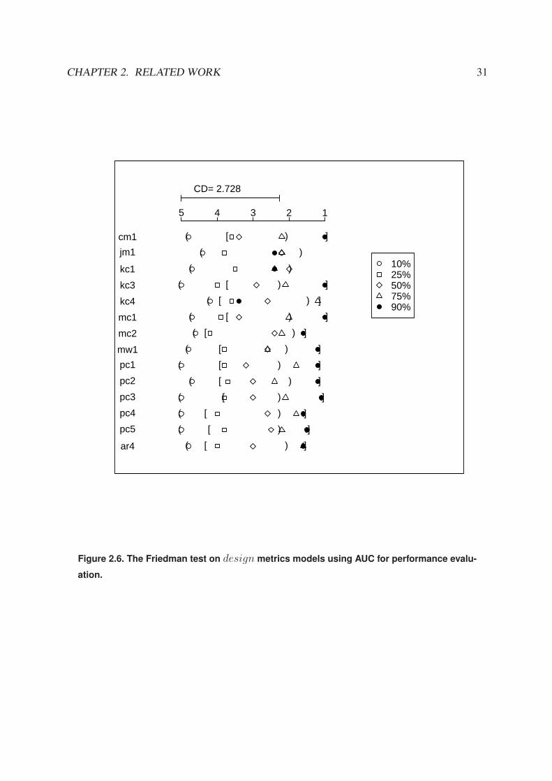
Let’s look at Figure 2.5. The numbers in the scale represent the average rank; the higher therank, the worse the performance of a training size. Therefore, from the worst towards the best,the order of models is from 10% to 90%. In Figure 2.5, the critical difference (CD) is 2.728.When the difference between two average ranks (or two models) is smaller than the value ofCD, the difference in their performance is not significant, as connected by a bold straight line.Figure 2.5 indicates that our fault prediction models form two performance clusters: one is 10%,25%, 50%, and 75%; the other is 25%, 50%, 75%, and 90%.
With more than one data set, we used a modified version of Demsar’s significance diagrams.Let’s compare Demsar’s significance diagram shown in Figure 2.5 to the first item (the same

CHAPTER 2. RELATED WORK 30
5 1 2 3 4
10% 25% 50%
75%
90%
CD = 2.728
Figure 2.5. An example of Demsar’s significance diagrams.
test on cm1 data) in Figure 2.6. The rank is still represented on a horizontal scale from 1 to5: the higher the rank, the worse the performance of a training size. CD still represents thecritical difference value for this statistical test. However, two straight lines are replaced withtwo bracket pairs: round and square bracket. The models inside each bracket do not have anystatistical difference. The round bracket forms the worst performance models while the bestperformance models are enclosed inside the square bracket. In this way, Figure 2.6 is able toshow the test result of 14 data sets.
2.5 MDP Data Sets and Prior Experiments
The 16 data sets used in this dissertation come from the NASA MDP repository [2] andPROMISE (3 data sets) [13] shown in Table 2.3. Metrics Data Program (MDP) is a softwaremetrics repository provided by NASA IV &V and is available to general users through websitehttp://mdp.ivv.nasa.gov/. MDP data stores and organizes the software product metrics data andassociated error data at the module (functional/method) level. Currently, there are 13 projectsdata available. All MDP data are also available from PROMISE [13] public repository. Publicfault data repository provide a possible platform for comparison of different approaches, dif-ferent measurements, and different research groups worldwide. With the availability of publicfault data sets, fault prediction are able to be investigated in a repeatable, or improvable, or evenrefutable way.
CHAPTER 2. RELATED WORK 31
CD= 2.728
12345
cm1 )( [ ]
jm1 )(
kc1 )(
kc3 )( [ ]
kc4 )( [ ]
mc1 )( [ ]
mc2 )( [ ]
mw1 )( [ ]
pc1 )( [ ]
pc2 )( [ ]
pc3 )( [ ]
pc4 )( [ ]
pc5 )( [ ]
ar4 )( [ ]
10%25%50%75%90%
Figure 2.6. The Friedman test on design metrics models using AUC for performance evalu-
ation.

CHAPTER 2. RELATED WORK 32
Table 2.3. Datasets used in this dissertationData mod.# % faulty project description lang. sourceJM1 10,878 19.3% Real time predictive ground system C MDP
MC1 9466 0.64% Combustion experiment of a space shuttle (C)C++ MDP
PC2 5589 0.42% Dynamic simulator for attitude control systems C MDP
PC5 17,186 3.00% Safety enhancement system C++ MDP
PC1 1109 6.59% Flight software from an earth orbiting satellite C MDP
PC3 1563 10.43% Flight software for earth orbiting satellite C MDP
PC4 1458 12.24% Flight software for earth orbiting satellite C MDP
CM1 505 16.04% Spacecraft instrument C MDP
MW1 403 6.7% Zero gravity experiment related to combustion C MDP
KC1 2109 13.9% Storage management for ground data C++ MDP
KC3 458 6.3% Storage management for ground data Java MDP
KC4 125 48% Ground-based subscription server Perl MDP
MC2 161 32.30% Video guidance system C++ MDP
ar3 63 12.70% Refrigerator C PROMISE
ar4 107 18.69% Washing machine C PROMISE
ar5 36 22.22% Dish washer C PROMISE

CHAPTER 2. RELATED WORK 33
Inside these MDP data sets, JM1 and KC1 have 21 attributes that can be used as pre-dictor variables, MC1 and PC5 have 39, the other data sets from MDP repository have 40.The 3 data sets from PROMISE [3] were collected from a Turkish white-goods manufac-turer building controller software for a washing machine, a dishwasher and a refrigerator, with29 variables. Although the names of variables from these 3 PROMISE data sets are differ-ent from MDP, they in fact are equivalent to a subset of metrics used in MDP repository.For example, metrics “total loc”, “unique operands”, and “halstead time” in PROMISE corre-spond to “loc total”,“num operands”, and “halstead prog time” in MDP. The metrics describ-ing PROMISE project are presented in bold font in Table 2.4.
The metrics shown in Table 2.4 have been extracted using McCabe IQ 7.1, a reverse engi-neering tool that derives software quality metrics from code, visualize flowgraphs and generatereport documents [1]. In all the data sets, available metrics are classified into three groups:design, code, and other, as indicated in Table 2.4. What separates design metrics from codemetrics is the opportunity to extract them from design specification diagrams such as UML.For example, Ohlsson and Alberg extract design metrics such as McCabe cyclomatic com-plexity from Formal Description Language (FDL) graphs [72]. Their design metrics includenode count, branch count, and McCabe cyclomatic complexity measures [72], also producedby McCabe IQ tool. McCabe complexity metrics are also used as design metrics in [91], thestudy that provides motivation and a point of comparison for this research. As a quick re-minder, if graph G represents module’s flowgraph, its cyclomatic complexity v(G) is calculatedas v(G) = e− n + 2, where e is the number of edges and n is the number of nodes.
The code metrics are the features that can only be extracted from the source code. Staticcode metrics, such as num operators,num oprands, and the Halstead metrics are calculatedfrom program statements [31, 34]. other metrics are those related to both design and code.Most data sets have four metrics we classified as other. We do not use other metrics in isolationto build models, but we include them in the experiments in which fault prediction models aredeveloped from all (also called module metrics) available attributes.
Guo et al. [33] build fault prediction modules using a set of classifiers on five MDP datasets(CM1, JM1, PC1, KC1, and KC2) and they find the random forest classifier has betterperformance than others inside this set of classifiers. Challagulla et al. [18] study 4 MDP datasets using 11 classifiers. Their findings show that there is no particular learning technique that

CHAPTER 2. RELATED WORK 34
Table 2.4. Metrics used.group metrics description or formula
code
parameter count Number of parameters to a given modulenum operators:N1 The number of operators contained in a modulenum operands:N2 The number of operands contained in a modulenum unique operators:µ1 The number of unique operators contained in a modulenum unique operands:µ2 The number of unique operands contained in a modulehalstead content:µ The halstead length content of a module µ = µ1 + µ2halstead length:N The halstead length metric of a module N = N1 + N2
halstead level:L The halstead level metric of a module L =(2∗µ2)µ1∗N2
halstead difficulty:D The halstead difficulty metric of a module D = 1L
halstead volume:V The halstead volume metric of a moduleV = N ∗ log2(µ1 + µ2)
halstead effort:E The halstead effort metric of a module E = VL
halstead prog time: T The halstead programming time metric of a moduleT = E
18halstead error est: B The halstead error estimate metric of a module
B = E2/31000
number of lines Number of lines in a moduleloc blank The number of blank lines in a moduleloc code and comment:NCSLOC The number of lines which contain both code and
comment in a moduleloc comments The number of lines of comments in a moduleloc executable The number of lines of executable code for a module
(not blank or comment)percent comments Percentage of the code that is commentsloc total The total number of lines for a given module
design
edge count:e Number of edges found in a given module fromone module to another
node count:n Number of nodes found in a given modulebranch count Branch count metricscall pairs Number of calls to functions in a modulecondition count Number of conditionals in a given modulecyclomatic complexity: v(G) The cyclomatic complexity of a module
v(G) = e− n + 2
decision count Number of decision points in a moduledecision density Condition count/Decision count
design complexity:iv(G) The design complexity of a module
design density Design density is calculated as: iv(G)v(G)
essential complexity:ev(G) The essential complexity of a module
essential density Essential density is calculated as: (ev(G)−1)(v(G)−1)
maintenance severity Maintenance Severity is calculated as: ev(G)v(G)
modified condition count The effect of a condition affect a decision outcome byvarying that condition only
multiple condition count Number of multiple conditions within a modulepathological complexity A measure of the degree to which a module contains
extremely unstructured constructs
others
normalized cylomatic complexity v(G)number of lines
global data complexity:gdv(G) the ratio of cyclomatic complexity of a module’sstructure to its parameter count
global data density Global Data density is calculated as: gdv(G)v(G)
cyclomatic density v(G)NCSLOC

CHAPTER 2. RELATED WORK 35
performs the best for all the data sets. However, some combination methods are the bettermethods that showed relatively better consistency in prediction accuracy compared with others.Mertik et al. [64] have the same results. Mertik et al. use so-called multimethods whichcombine decision tree C4.5, support vector machine, and genetic algorithms to predict softwarefault severity of three MDP projects, PC4, KC3, and KC4. And they show that combinationmultimethods are generally better than single algorithm method.
Feature Subset Selection (FSS) is investigated in MDP data sets too. Turhan et al. [83]use 8 MDP data sets to built fault prediction models using metrics which have been filtered byfeature subset selection (FSS) methods and those have not been filtered by FSS. They foundthe models which have been filtered by using FSS is better than those have not. Menzies etal. [62] and Guo [33] also apply FSS on MDP data sets, but they found in different data sets,the top five most important attributes vary with different data sets.
Menzies et al. [62] make the foundation of fault prediction studies on MDP data sets. Byusing a simple classifier naiveBayes, it is practical and useful to build fault prediction modelsfrom code metrics to guide software IV &V inspection, and they call for a better classifier forfault prediction. Lessmann et al. [53] investigated 22 classifiers over 10 data sets in MDPrepository, they found that most classifiers (18 out of 22) demonstrate the same performancestatistically.
Zhong et al. [92,93] are the first group who applied unsupervised learning in two MDP datasets: JM1 and KC2. They used Neural-Gas and K-means clustering to class software modulesinto several groups by using 13 module metrics. The clustered groups were then inspected byhuman experts to be fault-prone or not fault-prone. Their results indicate promising potentialfor the unsupervised learning method.
2.6 Heuristic
In this chapter, we review various metrics used in literature: requirement metrics, designmetrics, code metrics, and different social network metrics, for example, the developer infor-mation, messages about mailing list, and organizational structure complexity metrics. All thesemetrics are proved to be effective predictors for faults (or fault-proneness information). But,

CHAPTER 2. RELATED WORK 36
models built from these metrics are seldom combined and compared. Base on the best knowl-edge of the authors, the only work combining and comparing design and code metrics is Zhaoet al. [91]. They conclude that the design metrics are as good as the code metrics; little im-provement can be achieved if both design metrics and code metrics are used.... However, theirconclusions were drawn from the data analysis from a single software project using only onefault prediction modeling technique (logistic regression). One of our goals is to reexamine theirconclusion. In this dissertation, we use 14 publicly available project data sets. Each of theseprojects offers both design and static code metrics. We built fault prediction models using eachmetrics set separately (models denoted as design and code, respectively), as well as from acombined metrics data set (denoted as all). Chapter 3 will introduce our experiments to com-pare combine requirement metrics and module metrics (design and code metrics). Chapter 4will present our experiments and results on comparing and combining design and code metrics.
We also review all possible different types of evaluation methods for software fault pre-diction models. Inside these evaluation techniques, there have been attempts to include costfactors. F-measure, for example, offers a technique to account for the cost factor [39] whencomparing different models. Khoshgoftaar and Allen [49] proposed the use of prior probabili-ties of misclassification to select classifiers which offer the most appropriate performance. Costeffectiveness measures described by Arisholm et al. [7] can account for the nonuniform cost ofmodule-level V &V . However, there is no existing evaluation techniques can address a projectspecific misclassification cost or a module specific misclassification cost needs. Hence, we in-troduce a cost curve evaluation technique in Chapter 5 to address this special cost evaluation infault prediction models.

Chapter 3
Prediction from Requirement Metrics
In this chapter, we explore the following problems:
• Q1: Are requirement metrics good enough to build fault prediction models?• Q4: Do fault prediction models built from a combination of requirement, design, and
code metrics provide better performance than models built from any metric subset?
First, we begin with an introduction on the requirement metrics in MDP repository. Then, weshow our experimental design and result. We conclude with a summary and discussion.
Therefore, in this chapter, we investigate whether metrics available early in the developmentlifecycle can be used to identify fault-prone software modules. More precisely, we build pre-dictive models using the metrics that characterize structured textual requirements. We comparethe performance of requirements-based prediction models against the performance of module-based models. Finally, we develop a methodology that combines requirement and module met-rics. Since such models cannot be developed early in the lifecycle, we evaluate whether suchcombination can increase the prediction power in comparison to models that use module met-rics only. Using a range of modeling techniques and the data from three projects included inNASA Metrics Data Program (MDP) [2], CM1, JM1, and PC1, our experiments indicate thatthe early lifecycle metrics can play an important role in project management, either by pointingto the need for increased quality monitoring during the development or by using the models to
37

CHAPTER 3. PREDICTION FROM REQUIREMENT METRICS 38
assign verification and validation activities.
3.1 Static Requirements Features
The datasets used in this chapter is NASA Metrics Data Program (MDP) data repository [2].Although MDP repository contains 13 projects, only 3 of them offer requirement metrics. Thesethree projects are CM1, JM1, and PC1. From Table 2.3 we can see that CM1 project is a NASAspacecraft instrument, JM1 is a realtime ground system, PC1 is an earth orbiting satellite system.There are 10 attributes that describe requirements. One of them is the unique requirementidentifier. The remaining 9 attributes assume non negative integer values. These metrics areshown in Table 3.1. We use them as attributes when building fault prediction models.
All the MDP requirement metrics follow the definitions from Wilson [86]. According tothe reference, a tool “searches the requirements document for terms [the research at NASA-Goddard Software Assurance Research Center has] identified as quality indicators”. ARM(Automated Requirement Measurement) tool [86] was an experiment in lightweight parsing ofrequirements documents. Rather than to tackle the complexities of full-blown natural language,the ARM research explored what could be easily automatically identified. The ARM work re-sulted in an automatic parser and some threshold guidelines regarding when to be concernedabout a requirements document. Since our classification algorithms can automatically generatesuch thresholds, we ignored the ARM thresholds and just used the numerical values offered bythe parser.
The ARM parser reports information at the level of individual requirement specifications.Specification statements are evaluated along the following dimensions:
• Imperatives (something that must be provided) count the phrases “shall”, “must” or “mustnot”, “is required to”, “are applicable”, “responsible for”, “will”, or “should”.
• Continuances (connections between statements) count the phrases “as follows”, “follow-ing”, “listed”, “in particular”, or“support”.
• Directives (to supporting illustrations) count the phrases “figure”, “table”, “for example”,“note”.
• Options give the developer latitude in satisfying the specification statement. This count

CHAPTER 3. PREDICTION FROM REQUIREMENT METRICS 39
includes the phrases “can”, “may” and “optionally”.• Weak Phrases (causing uncertainty, leave room for multiple interpretations) count the
phrases “adequate”, “as a minimum”, “as appropriate”, “be able to”, “be capable”, “butnot limited to”, “capability of”, “capability to”, “ effective”, “if practical”, “normal”, “provide for”, “timely”, and “tbd”.
Table 3.1. Requirement Metrics.
Requirement Definitionsaction Represents the number of actions the requirement needs to be capable of performing.
conditional Represents whether the requirement will be addressing more than one condition.
continuance Phrases that follow an imperative and precede the definition oflower level requirement specification.
imperative Those words and phrases that command that something must be provided.
incomplete Phrases such as ‘TBD’ or ‘TBR’. They are used when a requirement has yetto be determined.
option Those words that give the developer latitude in the implementation of the specificationthat contains them.
risk level A calculated risk level metric based on weighted averages from metrics collected foreach requirement.
source Represents the number of sources the requirement will interface with or receive data from.
weak phrase Clauses that are apt to cause uncertainty and leave room for multiple interpretations.
3.2 Experimental Design and Result
3.2.1 Experimental Design
In this chapter, we report the development and evaluation of models to predict fault-pronesoftware modules using the following information from NASA MDP datasets [2]:
1. Experiment 1: Available metrics describing unstructured textual requirements;

CHAPTER 3. PREDICTION FROM REQUIREMENT METRICS 40
2. Experiment 2: Available software module metrics;
3. Experiment 3: A combination of requirement metrics and module metrics.
The goal of each of these experiments is different. In experiment 1, we try to assess howuseful the early lifecycle data and the related metrics are in identifying potentially problematicmodules. The second experiment is the least interesting from the research standpoint as the useof static module metrics in the prediction of faulty modules has been investigated extensively,even on the same datasets we use here. However, in our case, it sets the performance baselinefor the third experiment. We will demonstrate that the use of combined requirements metricsand static module metrics performs extremely well in predicting fault-prone modules.
In order to enable these experiments, we had to be able to relate individual requirementswith software modules. The generic structure of an entity relationship diagram that connectsrequirements with modules for a specific project entered in NASA MDP database is shown inFigure 3.1. All software requirements and modules are uniquely numbered. A requirement maybe implemented in one or more modules. A module implementation may reflect one or morerequirements. Further, a module may contain zero, one or more faults. For the purpose of ourexperiments, if a module contains any faults, it is considered fault-prone. Otherwise, it is faultfree. Unfortunately, MDP datasets [2] reveal anomalies too. Some requirements are associatedwith no software modules and some modules cannot be traced to any stated requirement. Asour research group has not been involved with the data collection, we could only point out tosuch inconsistencies. The extent of such inconsistencies is described later.
1 1
n
n
n
Figure 3.1. An entity-relationship diagram relates project requirements to modules and mod-
ules to faults
We combine requirement metrics and module metrics available for some of the projects inNASA Metrics Data Program (MDP) database [2]. Combining requirement metrics and module

CHAPTER 3. PREDICTION FROM REQUIREMENT METRICS 41
metrics if there is a one-to-one relationship between the requirements and modules is trivial.But, due to many-to-many relationship, we need to utilize the inner− join database operation.Inner-join, also referred in the literature as equijoin [75], results in merging the records fromtwo relational tables for which there is a matching value in the field(s) on which the tables arejoined. It creates an all-to-all association between the corresponding entries in two databasetables. This is the most common type of database join operation.
Referring to Figure 3.1, the inner-join takes all the records from CM1 product requirement metricstable and finds the matching record(s) in table CM1 requirement product relations based on thecommon predicate — Requirement ID. The result is written into a temporary table. Inner-joinfurther takes all the records from the temporary table and looks for the matching records inCM1 product module metrics via the join predicate Module ID. Table 3.2 shows partial resultsof this operation.
Table 3.2. The result of inner join on CM1 requirement and module metrics.Req id action Continuance Mod id loc blank Branch count ···100 1 0 25321 82 43 ···100 1 0 25333 34 17 ···101 3 1 25325 14 7 ···102 1 0 25321 82 43 ···102 1 0 25325 14 7 ···102 1 0 25333 34 17 ······ ··· ··· ··· ··· ···
As mentioned earlier, partial requirement metrics are available for the three MDP datasets:CM1, JM1 and PC1. In addition, our analysis uncovered several data discrepancies. Table 3.3summarizes the available data. In projects CM1 and PC1, only 22% and 18% of all modules,respectively, have their requirements identified. The extreme case is the dataset JM1 in whichonly 1% of modules are associated with any requirement. But, due to the fact that JM1 isthe largest project, the number of modules with identified requirements (97) is similar to thecorresponding value for PC1 (109). In experiments, we will consider only the subset of modulesin CM1, JM1 and PC1 which have their requirements identified. We will call these datasetsCM1 r, JM1 r and PC1 r, to separate them from their usage in existing literature [17, 33, 62].

CHAPTER 3. PREDICTION FROM REQUIREMENT METRICS 42
Table 3.3. The associations between modules and requirements in CM1, JM1 and PC1.
total modules with modules faulty modules total # req. related # of req.modules faults have req. with req. of req. to module(s) related to faults
CM1 r 505 81(16.03%) 109(22%) 58(53.21%) 160 114 69(60.53%)
JM1 r 10,878 2102 (19.32%) 97(1%) 4(4.12%) 74 17 3(17.65%)
PC1 r 1107 73(6.59%) 203(18%) 44(21.67%) 320 320 109(34.06%)
3.2.2 Prediction from Requirements Metrics
CM1 r dataset
CM1 r dataset describes software artifacts of a NASA spacecraft instrument. CM1 r has 160
requirements, but only 114 of them have associated program modules identified. Among these114 requirements, 69 (60.53%) of them are related to modules which contain at least one fault.This is a very significant percentage. On the other hand, only the modules with identifiedrequirements (109 of them out of 505) were used in the training/testing datasets.
As described in the Experimental Design section, we first developed models that predictdefective modules using the requirements metrics only. The performance of different machinelearning algorithms is depicted in the ROC curve shown in Figure 3.2. No model appears toprovide particularly useful information for project managers, which can probably be attributedto the fact that more than 60% of the requirements are related to defective modules.
JM1 r dataset
JM1 metrics represent a realtime ground system that uses simulations to generate flight pre-dictions. JM1 r has 74 requirements available (see Table 3.3). Only 17 of them are related toprogram modules. Three of these 17 requirements are associated to defective modules (17.65%).Figure 3.3 compares the performance of different models in an ROC curve. Although the per-formance of most models fails to provide useful information, the models built using Logistic

CHAPTER 3. PREDICTION FROM REQUIREMENT METRICS 43
0.0 0.2 0.4 0.6 0.8 1.0
0.0
0.2
0.4
0.6
0.8
1.0
CM1_r req.
PF
PD
IBkJ48LognbayesOneRVFIVP
RF
Figure 3.2. CM1 r prediction using requirements metrics only.
and VFI algorithms appear to do better than the others. Although JM1 is a very large project(> 10, 000 modules overall), JM1 r is very small as the information that relates requirementsand program modules is largely missing.
PC1 r dataset
PC1 project refers to an Earth orbiting satellite software system. PC1 r has 320 available re-quirements (Table 3.3) and, in contrast to CM1 r and JM1 r, all of them are associated withprogram modules. 109 (34.06%) requirements, or at least some aspect of these requirements,are implemented by modules which contain one or more faults. On the other hand, all theserequirements point to only 203 out of 1107 modules indicating, again, missing information.Consistent with our experimental design, we developed PC1 r models using the 320 require-ments and 203 modules.
The performance of PC1 r is shown in Figure 3.4. Unlike in the other two experiments, theuseful portion of the ROC curve is in the cost-adverse region with low false alarm rate (PF <
0.5), but coupled with the low probability of detection (PD < 0.5). If the data represented a

CHAPTER 3. PREDICTION FROM REQUIREMENT METRICS 44
0.0 0.2 0.4 0.6 0.8 1.0
0.0
0.2
0.4
0.6
0.8
1.0
JM1_r req.
PF
PD
IBkJ48LognbayesOneRVFIVP
RF
Figure 3.3. JM1 r prediction using requirements metrics only.
stable development environment in which this type of a model was built from an earlier project,the fact that the V&V team could start to develop information about modules in which faultscan be expected seems very encouraging. However, given that these are the first-of-the-kind,preliminary experiments with fault prediction models build from requirement metrics, we canonly cautiously suggest that our results warrant further research in this area.
3.2.3 Prediction from Static module metrics
As discussed, an extensive body of work describes fault prediction from module static mod-ule metrics. Therefore, the purpose of this section is to establish the baseline performance to beused for performance comparison throughout this proposal.
CM1 and PC1 projects contain 43 attributes. We removed 6 attributes that do not impact bi-nary classification: module id; two fault counting attributes: error count and error density;and the three attributes that have the same value for every module: global data complexity,global data density, and pathological complexity. We use the remaining 37 static moduleattributes in CM1 r and PC r. JM1 dataset comes with only 24 static module attributes. We

CHAPTER 3. PREDICTION FROM REQUIREMENT METRICS 45
0.0 0.2 0.4 0.6 0.8 1.0
0.0
0.2
0.4
0.6
0.8
1.0
PC1_r requirement
PF
PD
IbkJ48LognbayesOneRVFIVP
RF
Figure 3.4. PC1 r prediction using requirements metrics only.
removed the module identifier and two error related attributes and used remaining 21 modulemetrics for the classification.
The predicted class is always the presence of faults in a module (fault-free or faulty). A de-tailed description of module attributes can be found in [33, 62]. Several recent studies describethe fault prediction results for the NASA MDP datasets [17, 33, 62]. These studies provideinsights into the effects of feature (attribute) selection to model performance, as well as thevariations caused by the use of a wide spectrum of machine learning algorithms. The observa-tion has been that the choice of learning methods have a much stronger impact on performancethan feature selection [62].
Although CM1, JM1 and PC1 have static module metrics data available for all modules(505, 10, 878 and 1, 107, respectively), to make performance comparisons fair, we only usemodules that explicitly correspond to requirements (109, 97, 203, respectively). Therefore, theperformance results embodied by the ROC curves in this chapter are not the same as reportedin related literature [17, 33, 62], but similar.
Figures 3.5, 3.6 and 3.7 depict the performance of fault prediction models based on module

CHAPTER 3. PREDICTION FROM REQUIREMENT METRICS 46
0.0 0.2 0.4 0.6 0.8 1.0
0.0
0.2
0.4
0.6
0.8
1.0
CM1_r module
PF
PD
IBkJ48LognbayesOneRVFIVP
RF
Figure 3.5. CM1 r using module metrics.
metrics. Machine learning algorithms provide models in the different regions of the ROC space.While the performance on neither of the project datasets appears impressive, consistent with thetrends observed in related studies, JM1 r dataset proves extremely difficult. Among those whouse NASA MDP datasets, JM 1 has been suspected of containing noisy (inaccurate) informa-tion. But while its large size usually makes it challenging for fault prediction, in our experimentJM1 r contains only 97 modules, with 4 of them being defective. Therefore it comes as nosurprise that most machine learning algorithms (all except the random forest) generate theoriesthat classify all the modules as fault-free.
The machine learning algorithms which typically perform better than others are randomforests, naive bayes, and IBk, although the usefulness of their predictions in the context ofsoftware engineering projects appears rather limited.
3.2.4 Combining Requirement and Module Metrics
We combine requirement and module metrics using the inner-join method described ear-lier. Recall that there are 109, 97 and 203 modules associated to requirements in CM1, JM1

CHAPTER 3. PREDICTION FROM REQUIREMENT METRICS 47
0.0 0.2 0.4 0.6 0.8 1.0
0.0
0.2
0.4
0.6
0.8
1.0
JM1_r module
PF
PD
IBkJ48LognbayesOneRVFIVP
RF
Figure 3.6. JM1 r using module metrics.
and PC1 datasets, respectively. When many-to-many relationship exists between modules andrequirements, the inner join creates multiple entries in the resulting table, one for each uniqueRequirement ID and Module ID pair. Consequently, the datasets used in this experiment arelarger. CM1 RM has 266 records, while PC1 RM has 477 records. JM1 RM maintained thesame number of records, 97 because each module is related to a single requirement. The numberof defective modules in each dataset remains the same as in the previous experiments; 147 faultyrecords for CM1 RM, only 4 for JM1 RM, and 111 for PC1 RM, but multiple fault records mayexist for a single module.
Following the preparation of data set, we ran the 5 way cross-validation. First, we dividea dataset into five bins. Then we use four bins of data to train classifiers and build models, astandard experimental procedure. But, the dataset may contain multiple entries for the samemodule, if it is related to more than one requirement. To avoid counting the classification ofthe same module more than once, in the fifth bin – the testing bin, we must ensure that it onlycontains unique modules. In other words, we eliminate multiple entries of the same moduleand randomly keep one entry for each module. Finally, comparing the ground truth with theclassification outcomes, we ascertain PD and PF and generate an ROC curve.

CHAPTER 3. PREDICTION FROM REQUIREMENT METRICS 48
0.0 0.2 0.4 0.6 0.8 1.0
0.0
0.2
0.4
0.6
0.8
1.0
PC1_r module
PF
PD
IbkJ48LognbayesOneRVFIVP
RF
Figure 3.7. PC1 r using module metrics.
The prediction results for CM1 RM are shown in Figure 3.8 and for PC1 RM in Figure3.9. The presence of additional requirement metrics attributes in JM1 RM did not improve theprediction model which used module metrics only. Both JM1 r and JM1 RM have the samenumber of entries, 97, which explains the lack of performance gains.
3.3 Discussion
Upon seeing the results of the experiments that combine requirements and static modulemetrics, we were pleasantly surprised. A nearly 70% improvement of PD at PF = 0.1 ob-served in CM1 r dataset, for example, is very significant. We have been building models forfault prediction in NASA MDP datasets for several years. A recent publication [62] reportsthat the best model performance based on module metrics only is (PD = 71%, PF = 27%)
for CM1 dataset and is (PD = 48%, PF = 17%) for PC1. Our own experiments with mod-ule metric models reported in this chapter reflect the use of subsets of CM1, JM1 and PC1project data and are somewhat different. But the performance improvement gained by addingrequirements metrics has surpassed all our expectations. Figures 3.10, 3.11 and 3.12 depict

CHAPTER 3. PREDICTION FROM REQUIREMENT METRICS 49
0.0 0.2 0.4 0.6 0.8 1.0
0.0
0.2
0.4
0.6
0.8
1.0
CM1_r mod+req (innerjoin)
PF
PD
IBkJ48LognbayesOneRVFIVP
RF
Figure 3.8. CM1 RM model uses requirements and module metrics.
ROC curves for the three datasets, CM1, JM1 and PC1, respectively. Depicted models havebeen developed using the random forests algorithm. Random forests have demonstrated themost consistent performance in all our experiments and we believe it is appropriate to use themfor performance comparison. Each of these three figures contains three lines, depicting theperformance of requirements-only based model, the module-only based model and, finally, themodel that combines requirements and module metrics.
These results demand a careful analysis. Our first observation is specific and it relates to theinner workings of machine learning algorithms we used for modeling. After the inner-join, thedatasets have more records. In other words, the datasets became oversampled. Oversamplingis known to be an effective method in signal processing. Recent studies show that tree-basedclassifiers do not increase the performance as the result of oversampling in the training data [24,25]. Random forests is a tree based ensemble-forming algorithm. So our results appear tocontradict the results of Drummond and Holte in [24,25]. Why random forests perform so wellon the inner-join data? This phenomenon certainly is worth exploring in the future. However,other learners we used such as J48 and IBk, also improve their performance when requirementsand module metrics are combined. Therefore, the observed performance improvement cannot

CHAPTER 3. PREDICTION FROM REQUIREMENT METRICS 50
0.0 0.2 0.4 0.6 0.8 1.0
0.0
0.2
0.4
0.6
0.8
1.0
PC1_r mod+req (innerjoin)
PF
PD
IBkJ48LognbayesOneRVFIVP
RF
Figure 3.9. PC1 RM model uses requirements and module metrics.
be explained through better understanding of the algorithms behind specific machine learnersonly.
The obvious speculation here is that the training/test datasets after the inner-join representreal world software engineering situations better. Our experiments provide initial evidencethat combining metrics that describe different yet related software artifacts may significantlyincrease the effectiveness of fault prediction models. Although each metric, regardless whetherit describes requirement or module features, appears highly abstract and seemingly unrelated tosoftware faults, when combined, they support the development of what appear to be superiorfault prediction models.
We need to add a few caveats. NASA MDP is a continually growing dataset of softwareengineering data. The data we were able to obtain for the three projects do not appear to behighly accurate. As we mentioned, there are many requirements with no corresponding modulesand, even more concerning, many modules with no corresponding requirements. We believe tohave alleviated this problem by limiting our experiments to only include modules which haveidentified links to requirements. But as a result, we have models designed for a subset of project

CHAPTER 3. PREDICTION FROM REQUIREMENT METRICS 51
0.0 0.2 0.4 0.6 0.8 1.0
0.0
0.2
0.4
0.6
0.8
1.0
Comparison of ROC curves of CM1_r
PF
PD
reqmodinnerjoin
Figure 3.10. ROC curves for CM1 project.
0.0 0.2 0.4 0.6 0.8 1.0
0.0
0.2
0.4
0.6
0.8
1.0
Comparison of ROC curves of JM1_r
PF
PD
reqmodinnerjoin
Figure 3.11. ROC curves for JM1 project.

CHAPTER 3. PREDICTION FROM REQUIREMENT METRICS 52
0.0 0.2 0.4 0.6 0.8 1.0
0.0
0.2
0.4
0.6
0.8
1.0
Comparison of ROC curves of PC1_r
PF
PD
reqmodinnerjoin
Figure 3.12. ROC curves for PC1 project.
data. These subsets have a higher proportion of faulty entries than the the datasets representingprojects they come from. Machine learning algorithms generally perform better on smallerdatasets. They also perform better on data sets where the size difference between majority andminority classes is insignificant. Therefore, our results are encouraging, but they may be overlyoptimistic.
3.4 Summary
In this chapter, we describe fault prediction models built using metrics extracted from un-structured textual requirements, the module (/product) metrics, and the fused requirement andmodule metrics. The models were developed and evaluated using metrics data from three NASAMDP projects: CM1, JM1, and PC1. Model comparison shows that requirement metrics can behighly useful for fault prediction. Although the requirement metrics do not predict faults wellby themselves, they significantly improve the performance of the prediction models that com-bine requirement and module metrics together using the inner-join method. Our experiments

CHAPTER 3. PREDICTION FROM REQUIREMENT METRICS 53
suggest that the early lifecycle metrics can play an important role in project management, eitherby pointing to the need for increased quality monitoring during the development or by using themodels to assign verification and validation activities.
Lastly, we address the questions Q1 and Q4:
• Q1: Are requirement metrics good enough to build fault prediction models?Answer: No. The requirement metrics extracted from textual description alone are notsufficient to predict software fault proneness.
• Q4: Do fault prediction models built from a combination of requirement, design, andcode metrics provide better performance than models built from any metrics subset?Answer: The combination of requirement metrics and module metrics are surprisinglygood at fault proneness prediction. Combination models are much better than the modelsfrom requirement and module metrics alone.

Chapter 4
Incremental Development of SoftwareFault Prediction Models
In this chapter, we investigate the following problems:
• Q2: Are design metrics good enough to be fault predictors?• Q3: Are code metrics good fault-prone predictors?• Q4:Do fault prediction models built from a combination of requirement, design, and code
metrics provide better performance than models built from any metrics subset?• Q5: How large is a training subset needed to build meaningful fault prediction models?• Q6: How large is a training subset needed to achieve the best performance fault prediction
model?
This chapter is organized as follows. First, we begin with the experimental design. Second,we show the experimental results. Finally, we discuss the results obtained in this chapter.
4.1 Experimental Design
The metrics shown in Table 2.4 have been extracted using McCabe IQ 7.1, a reverse engi-neering tool that derives software quality metrics from code, visualize flowgraphs and generate
54

CHAPTER 4. INCREMENTAL DEVELOPMENT OF SOFTWARE FAULT PREDICTION MODELS55
report documents [1]. It is important to note that McCabe IQ reverse engineers design metricsfrom code flowgraphs, rather than from design documentation. It is not unusual to analyzesoftware design quality from design artifacts reengineered from the code [5, 6, 15, 16, 81, 82].However, we recognize that this fact is one of the validity threats for our experiment.
The critical issue to be asked is whether the attributes listed in Table 2.4 as design met-rics can be obtained before coding begins. We believe all of these measures can be obtainedfrom detailed design documents, PSPEC descriptions for example, as long as such descriptionscan be used to build call-graphs and control-flow-graphs. A similar argument has been madenumerous times in the software engineering literature. According to Fenton and Pfleeger, Mc-Cabe metrics represent the structure of software product [31]. Fenton and Ohlsson [29] furtherstate:“(McCabe) complexity metrics is the rather misleading term used to describe a class ofmeasures that can be extracted directly from source code. Occasionally and more beneficially,(McCabe) complexity metrics can be extracted before code is produced, such as when the de-tailed designs are represented in a graphical language”. Ohlsson and Alberg extracted designmetrics from Formal Design Language (FDL) graphs [72]. Please note that these are the samemetrics we designate as design metrics.
The experiments conducted in this chapter use 14 data sets listed in Table 2.3 including all13 data sets from MDP and ar4 from PROMISE data repository. ar4 data set has 29 attributesincluding 9 design metrics, 18 code metrics, and 2 metrics classified as other.
4.1.1 Design of Experiments
Our goal is to investigate development of fault prediction models throughout the design andimplementation phases of the life cycle yields models with improved performance. There aretwo interesting aspects of incremental model development:
1. Utilization of the increasing number of modules as training data, and
2. Timely (sequential) utilization of design and code metrics.
To reach these goals, we will compare the performance of models derived from:

CHAPTER 4. INCREMENTAL DEVELOPMENT OF SOFTWARE FAULT PREDICTION MODELS56
• different percentages of data for model development (training): 10%, 25%, 50%, 75%,and 90%. In each experiment, the reminder of the data set will be used for model evalua-tion.
• different metric group: design, code, and all
The data sets we used do not include development schedule information. Therefore, wecannot faithfully emulate the actual “arrival” schedule of modules and their metrics. However,we will deploy cross-validation, the statistical practice of randomly partitioning a sample ofdata into two subsets:training and testing ten times. Reporting the median result from the tenexperiments should minimize the impact a development sequence could have on the predictionresults. The predicted variable is DEFECT , that is, the models predict whether a module islikely to contain fault(s).
Cross-validation is the statistical practice of randomized partitioning of a data sample intotwo subsets, one for model development (training) and the other for model testing. 10 waycross validation implies that each experiment is repeated 10 times, using different training andtesting subsets. As the size of training subset varies, for example, between 10%, and 90%,in our experiments the corresponding testing subset includes all the remaining data, i.e., 90%,down to 10% of the data set. All experiments undergo 10 repetitions, with no adjustmentsbased on sample sizes. Due to 10-way cross validation, comparing a large number of ROCcurves becomes difficult. For this reason, we visualize the ten corresponding values of AUC ina Box-plot diagram.
We will use 5 algorithms for software quality prediction: random forest, bagging, logisticregression, boosting, and NaiveBayes. These algorithms have consistently been recommendedto practitioners and provide adequate performance [39–43]. More importantly, the classifiersare implemented in publicly available machine learning toolkit Weka [87]. The use of multiplemachine learning algorithms allows us to compare the results with the recent study conductedby Lessman et al. [53], in which they compare the performance of two dozen classificationalgorithms on MDP data sets. We use the default parameters in all the classifiers except inrandom forest, in which we follow the recommendation of algorithm’s creator L. Breiman [14]and use 500 tree ensemble (rather than Weka default of 10 trees, which optimizes run-time).

CHAPTER 4. INCREMENTAL DEVELOPMENT OF SOFTWARE FAULT PREDICTION MODELS57
In total, we conducted 10,500 experiments utilizing 14 data sets, 5 different sizes of trainingsubset, 3 metrics groups, 10 cross validation runs, all of these repeated using 5 classificationalgorithms.
4.2 Experimental Results
4.2.1 Increasing the size of training set
One of the questions that repeatedly surface in discussions about fault prediction modelingdeals with the amount of data needed to build reasonably accurate models. The question isnot critical when models from earlier releases are used in the quality assurance of the newversion or product release. Presumably, such systems are part of the product line and faultprediction models from earlier releases are adequate for the new release [74]. However, when anorganization develops one-of-kind system or the first system release with no substantial history(and limited reuse), the amount of data needed to develop the models is the real issue in practice.This is certainly the case for most of the projects described in the NASA MDP repository. Wewill not directly address the “minimal” data set requirement for model development. Rather,following the idea of incremental model development, we would like to know the rate of modelimprovement as additional modules and their metrics descriptors become available.
For these reasons, we compare the performance of models generated using five training sub-set, containing 10%, 25%, 50%, 75%, and 90% of project modules. Although these proportionsrepresent different sizes of training data for different projects, they match realistic milestonesin the development life cycle.
We will test the following statistical hypotheses:H10:The size of the model’s training set has no influence on model performance.vs.H1α: Some (at least two) models developed using different training subset sizes result in signif-icantly different performance.

CHAPTER 4. INCREMENTAL DEVELOPMENT OF SOFTWARE FAULT PREDICTION MODELS58
For this experiment, we utilize 14 data sets, 5 different training subsets, 3 groups of met-rics,and 5 different machine learners, 10 times cross validation runs. Due to the sheer volumeof information, Demsar’s statistical analysis procedure [23] will provide acceptable summa-rization of results. The results are shown separately for models that utilize design metrics only,code metrics only, and all metrics.
The general trends to be reported are not surprising:
• 10% training subset results in the weakest performance.• In most cases, the “best” performance can be expected from models which use 90% of
data for training. Unfortunately, these models are the least useful as only 10% of themodules are left for fault prediction.
• Models increase their performance as the size of the training data set grows. However,these increases are rather minimal and statistical significance must be considered.
A more detailed analysis of the experimental results, including their statistical significanceand practical implications follows.
Design metrics models
We test the null hypothesis first on fault prediction models that use only design metrics.
Figure 2.6 shows the test result of 14 data sets measured by AUC using Demsar test proce-dure. The rank is represented on a horizontal scale from 1 to 5: the higher the rank is, the worsethe performance of the model. CD represents the critical difference value for this statisticaltest: if the difference between two ranks is greater than the value of CD, they are statisticallydifferent, otherwise, they are not. To account for the statistical significance, we enclose the fivemodels from each project into two pairs of brackets. Each bracket pair encloses the distanceequivalent to the value of CD = 2.728. The round brackets enclose models which from a per-formance cluster with the worst performing model (typically the model which trains from the10% subset). We will call this cluster the lower rank cluster. The square brackets enclose theperformance cluster which includes the best performing model (typically inferred from the 90%
subset). This will be our higher rank cluster.

CHAPTER 4. INCREMENTAL DEVELOPMENT OF SOFTWARE FAULT PREDICTION MODELS59
Let us look closely into the performance of the five models built from cm1 in Figure 2.6.For the increasing sizes of training subsets, the corresponding ranks are 4.8, 3.6, 3.4, 2.2, and 1.These ranks form two performance clusters. Models built from 25%, 50%, and 75% subsets arein the intersection between the lower and higher performance rank clusters. The fault predictionmodels for projects jm1 and kc1 exhibit no statistically significant differences regardless of thesize of the training subset. Therefore, they are included in a single performance rank cluster.The models for all other projects form two performance rank clusters. It is also interestingto note that in project kc4, the best performing model is developed using 75% of modules fortraining. In smaller projects (kc4 contains only 125 modules), training from 90% may result inover-fitting.
There are never more than two performance clusters. More detailed result comparisons inTable 4.1 and in Figure 4.1 will describe only 10%, 50%, and 90% training subsets.
Table 4.1. Median(m) and variance(v) of 10%, 50%, and 90% training subset models from
design metrics, measured by AUC
data m10% v10% m50% v50% m90% v90%m50%
m10%− 1 m90%
m10%− 1 m90%
m50%− 1
cm1 0.54 0.0035 0.57 0.002 0.60 0.0133 5.56% 11.11% 5.26%jm1 0.66 9e-04 0.67 8e-04 0.66 0.0013 1.52% 0 -1.49%kc1 0.72 0.0027 0.73 9e-04 0.73 0.0028 1.39% 1.39% 0kc3 0.61 0.0194 0.74 0.0121 0.77 0.0170 21.31% 26.23% 4.05%kc4 0.75 0.0109 0.78 0.0017 0.76 0.0175 4.00% 1.33% -2.56%mc1 0.53 0.0054 0.62 0.0091 0.68 0.0214 16.98% 28.30% 9.68%mc2 0.60 0.0087 0.63 0.0035 0.63 0.0271 5.00% 5.00% 0mw1 0.66 0.0163 0.76 0.0038 0.78 0.0282 15.15% 18.18% 2.63%pc1 0.57 0.0067 0.66 0.0028 0.69 0.0118 15.79% 21.05% 4.55%pc2 0.50 0.0269 0.67 0.0174 0.75 0.0503 34.00% 50.00% 11.94%pc3 0.65 0.0033 0.73 8e-04 0.73 0.0041 12.31% 12.31% 0pc4 0.73 0.0029 0.78 0.001 0.78 0.0036 6.85% 6.85% 0pc5 0.94 9e-04 0.95 1e-04 0.95 3e-04 1.06% 1.06% 0ar4 0.62 0.0185 0.70 0.0085 0.72 0.0803 12.9% 16.13% 2.86%

CHAPTER 4. INCREMENTAL DEVELOPMENT OF SOFTWARE FAULT PREDICTION MODELS60
Table 4.1 shows median and variance values for 10%, 50%, and 90% of data as trainingsubsets. The median value is rounded to two digits, variance to 4 digits. The last three columnsshow the percentage increase in model performance. If the performance increases, the valueis positive. Table 4.1 provides a closer look into the actual performance differences betweenmodels.
Figure 4.1 shows boxplot diagrams for 10%, 50%, and 90% of data as training subsets ondesign metrics which give a more intuitive view of comparison of these models.
Taken together from Table 4.1, Figure 4.1 and Figure 4.1, we can see that the gains in faultprediction vary from project to project and they are generally difficult to anticipate. Clearly,the significance results indicate that building only one or two models over the development lifecycle, given that only design metrics are utilized, should be sufficient.
Code metrics models
We repeated the same statistical analysis procedure for the models derived from code metrics.From Figure 4.2, we can see that:
1. For 8 data sets, lower cluster includes models developed from 10% to 50% of modules.
2. For 6 data sets, lower cluster includes models developed from 10% to 75% of modules.
3. For 5 data sets, the higher cluster includes models developed from 50% to 90%.
4. For 9 data sets, the higher cluster includes models developed from 25% to 90%.
Table 4.2 shows median and variance values of the AUC built from 10%, 50%, and 90%of data as training subsets. Figure 4.3 shows the corresponding boxplot diagrams. We notethat performance increases due to the growing size of training samples in code metrics basedfault prediction models are more modest than in case of models built from design metrics.However, the magnitude of performance improvement varies between projects and its difficultto anticipate.

CHAPTER 4. INCREMENTAL DEVELOPMENT OF SOFTWARE FAULT PREDICTION MODELS61
1 5 9
0.4
0.6
0.8
1.0
cm1
AU
C
1 5 9
0.4
0.6
0.8
1.0
jm1
AU
C
1 5 9
0.4
0.6
0.8
1.0
kc1
AU
C
1 5 9
0.4
0.6
0.8
1.0
kc3
AU
C
1 5 9
0.4
0.6
0.8
1.0
kc4
AU
C
1 5 9
0.4
0.6
0.8
1.0
mc1
AU
C
1 5 9
0.4
0.6
0.8
1.0
mc2
AU
C
1 5 9
0.4
0.6
0.8
1.0
mw1
AU
C
1 5 9
0.4
0.6
0.8
1.0
pc1
AU
C
1 5 9
0.4
0.6
0.8
1.0
pc2
AU
C
1 5 9
0.4
0.6
0.8
1.0
pc3
AU
C
1 5 9
0.4
0.6
0.8
1.0
pc4
AU
C
1 5 9
0.4
0.6
0.8
1.0
pc5
AU
C
1 5 9
0.4
0.6
0.8
1.0
ar4
AU
C
Figure 4.1. Boxplot diagrams of using 10%, 50%, and 90% data as training subset on design
metrics, measured by AUC . In x-axis, “1” stands for 10%; “5” stands for 50%; “9” stands
for 90%.

CHAPTER 4. INCREMENTAL DEVELOPMENT OF SOFTWARE FAULT PREDICTION MODELS62
CD= 2.728
12345
cm1 )( [ ]
jm1 )( [ ]
kc1 )( [ ]
kc3 )( [ ]
kc4 )( [ ]
mc1 )( [ ]
mc2 )( [ ]
mw1 )( [ ]
pc1 )( [ ]
pc2 )( [ ]
pc3 )( [ ]
pc4 )( [ ]
pc5 )( [ ]
ar4 )( [ ]
10%25%50%75%90%
Figure 4.2. The Friedman test on code metrics models evaluated using AUC.

CHAPTER 4. INCREMENTAL DEVELOPMENT OF SOFTWARE FAULT PREDICTION MODELS63
1 5 9
0.4
0.6
0.8
1.0
cm1
AU
C
1 5 9
0.4
0.6
0.8
1.0
jm1
AU
C
1 5 9
0.4
0.6
0.8
1.0
kc1
AU
C
1 5 9
0.4
0.6
0.8
1.0
kc3
AU
C
1 5 9
0.4
0.6
0.8
1.0
kc4
AU
C
1 5 9
0.4
0.6
0.8
1.0
mc1
AU
C
1 5 9
0.4
0.6
0.8
1.0
mc2
AU
C
1 5 9
0.4
0.6
0.8
1.0
mw1
AU
C
1 5 9
0.4
0.6
0.8
1.0
pc1
AU
C
1 5 9
0.4
0.6
0.8
1.0
pc2
AU
C
1 5 9
0.4
0.6
0.8
1.0
pc3
AU
C
1 5 9
0.4
0.6
0.8
1.0
pc4
AU
C
1 5 9
0.4
0.6
0.8
1.0
pc5
AU
C
1 5 9
0.4
0.6
0.8
1.0
ar4
AU
C
Figure 4.3. Boxplot diagrams of fault prediction models built from 10%, 50%, and 90% of
data using code metrics, measured by AUC . In x-axis, “1” stands for 10%; “5” stands for
50%; “9” stands for 90%.

CHAPTER 4. INCREMENTAL DEVELOPMENT OF SOFTWARE FAULT PREDICTION MODELS64
Table 4.2. Median(m) and variance(v) for models trained from 10%, 50%, and 90% of modules
using code metrics, measured by AUC .
data m10% v10% m50% v50% m90% v90%m50%
m10%− 1 m90%
m10%− 1 m90%
m50%− 1
cm1 0.61 0.0054 0.69 0.0019 0.72 0.0112 13.11% 18.03% 4.35%jm1 0.69 1e-04 0.72 2e-04 0.72 7e-04 4.35% 4.35% 0kc1 0.77 0.0011 0.80 3e-04 0.80 0.0017 3.90% 3.90% 0kc3 0.68 0.0212 0.78 0.0041 0.84 0.0273 14.71% 23.53% 7.69%kc4 0.57 0.0088 0.62 0.0082 0.65 0.0240 8.77% 14.04% 4.84%mc1 0.79 0.0150 0.92 0.0065 0.94 0.0092 16.46% 18.99% 2.17%mc2 0.61 0.0066 0.67 0.0032 0.70 0.0224 9.84% 14.75% 4.48%mw1 0.71 0.0160 0.79 0.0047 0.84 0.0281 11.27% 18.31% 6.33%pc1 0.70 0.0103 0.80 0.0037 0.83 0.0113 14.29% 18.57% 3.75%pc2 0.59 0.0341 0.80 0.0139 0.89 0.0338 35.59% 50.85% 11.25%pc3 0.75 0.0025 0.81 5e-04 0.82 0.0036 8.00% 9.33% 1.23%pc4 0.84 0.0046 0.90 0.0036 0.90 0.0055 7.14% 7.14% 0pc5 0.93 5e-04 0.95 3e-04 0.95 5e-04 2.15% 2.15% 0ar4 0.70 0.0293 0.79 0.0089 0.81 0.0853 12.86% 15.71% 2.53%
All metrics
All metrics refers to the entire set of module attributes available for each fault prediction dataset. These attributes include design and code metrics, as well as some software measures thatcombine them. The results of the ranking analysis for the incremental learning experiment withall metrics, using AUC for performance evaluation, are shown in Figure 4.4. A quick summaryfollows:
1. Regardless of the evaluation technique, jm1 does not show statistically significant differ-ence for any training methods.
2. There are 10 data sets for which the lower cluster includes 10% to 50% subsets of avail-able modules: cm1, kc1, kc4, mc1, mc2 pc1, pc2, pc4, pc5, ar4.

CHAPTER 4. INCREMENTAL DEVELOPMENT OF SOFTWARE FAULT PREDICTION MODELS65
CD= 2.728
12345
cm1 )( [ ]
jm1 )(
kc1 )( [ ]
kc3 )( [ ]
kc4 )( [ ]
mc1 )( [ ]
mc2 )( [ ]
mw1 )( [ ]
pc1 )( [ ]
pc2 )( [ ]
pc3 )( [ ]
pc4 )( [ ]
pc5 )( [ ]
ar4 )( [ ]
10%25%50%75%90%
Figure 4.4. The Friedman test on all metrics using AUC.

CHAPTER 4. INCREMENTAL DEVELOPMENT OF SOFTWARE FAULT PREDICTION MODELS66
3. There are 3 data sets for which the lower cluster includes models trained from 10% to75%: kc3, mw1, and pc3.
4. There are 7 data sets for which the higher cluster includes models trained from 50% to90% subsets: kc3, mc1, pc1, pc2, pc3, pc5, and ar4.
5. There are 6 data sets for which the higher performance cluster is from 25% to 90%: cm1,kc1, kc4, mc2, mw1, and pc4.
Table 4.3. Median(m) and variance(v) of models built from 10%, 50%, and 90% of module
using all metrics, measured by AUC
data m10% v10% m50% v50% m90% v90%m50%
m10%− 1 m90%
m10%− 1 m90%
m50%− 1
cm1 0.64 0.0047 0.72 0.0018 0.75 0.0084 12.50% 17.19% 4.17%jm1 0.69 1.00E-04 0.72 3.00E-04 0.72 9.00E-04 4.35% 4.35% 0kc1 0.76 0.0018 0.80 2.00E-04 0.80 0.0018 5.26% 5.26% 0kc3 0.65 0.0177 0.76 0.0131 0.79 0.0263 16.92% 21.54% 3.95%kc4 0.74 0.0104 0.81 0.0025 0.81 0.0132 9.46% 9.46% 0mc1 0.80 0.0176 0.95 0.0058 0.97 0.0069 18.75% 21.25% 2.11%mc2 0.62 0.0063 0.69 0.0042 0.70 0.0174 11.29% 12.90% 1.45%mw1 0.70 0.0182 0.78 0.0049 0.84 0.0234 11.43% 20.00% 7.69%pc1 0.70 0.0077 0.79 0.0028 0.83 0.0074 12.86% 18.57% 5.06%pc2 0.59 0.0313 0.83 0.0229 0.88 0.0254 40.68% 49.15% 6.02%pc3 0.74 0.0048 0.81 0.0011 0.82 0.0034 9.46% 10.81% 1.23%pc4 0.85 0.003 0.91 0.0013 0.92 0.0024 7.06% 8.24% 1.10%pc5 0.94 0.0012 0.96 2.00E-04 0.96 3.00E-04 2.13% 2.13% 0ar4 0.70 0.0275 0.78 0.0078 0.83 0.0781 11.43% 18.57% 6.41%
Table 4.3 shows median and variance values of AUC for models built from 10%, 50%, and90% of data as training subsets, as well as their comparison. Figure 4.5 shows the correspondingboxplot diagrams. An interesting observation inferred is that in case of comprehensive metricsattributes, fault prediction models never degrade when the size of the training set grows. This issimilar to code metrics models, but different from models which use design information only.

CHAPTER 4. INCREMENTAL DEVELOPMENT OF SOFTWARE FAULT PREDICTION MODELS67
1 5 9
0.4
0.6
0.8
1.0
cm1
AU
C
1 5 9
0.4
0.6
0.8
1.0
jm1
AU
C
1 5 9
0.4
0.6
0.8
1.0
kc1
AU
C
1 5 9
0.4
0.6
0.8
1.0
kc3
AU
C
1 5 9
0.4
0.6
0.8
1.0
kc4
AU
C
1 5 9
0.4
0.6
0.8
1.0
mc1
AU
C
1 5 9
0.4
0.6
0.8
1.0
mc2
AU
C
1 5 9
0.4
0.6
0.8
1.0
mw1
AU
C
1 5 9
0.4
0.6
0.8
1.0
pc1
AU
C
1 5 9
0.4
0.6
0.8
1.0
pc2
AU
C
1 5 9
0.4
0.6
0.8
1.0
pc3
AU
C
1 5 9
0.4
0.6
0.8
1.0
pc4
AU
C
1 5 9
0.4
0.6
0.8
1.0
pc5
AU
C
1 5 9
0.4
0.6
0.8
1.0
ar4
AU
C
Figure 4.5. Box-plot diagrams of fault prediction models built from 10%, 50%, and 90% of
data using all metrics, measured by AUC . In x-axis, “1” stands for 10%; “5” stands for
50%; “9” stands for 90%.

CHAPTER 4. INCREMENTAL DEVELOPMENT OF SOFTWARE FAULT PREDICTION MODELS68
The analysis of all the experiments leads to the following perspective. Regardless of thetype of metrics used for model development (design, code, and all), fault prediction modelsshould be built as early as an initial set of modules becomes available. Using 10% of projectmodules for model development results in models that, when statistical significance is takeninto account, are outperformed only by models built from 90% of the modules. Larger trainingset generally helps improve model performance, but the cost of incremental model rebuildingshould be compared with the performance benefits. When justified, model rebuilding does notneed to be a continual or a frequent activity. Rather, models could be built early and, possibly,updated at the mid point of the development.
4.2.2 Comparison of design, code, and all metrics models
The increase in size of available data for model definition is only one aspect in the incre-mental development of fault prediction models. The other opportunity comes from the fact thatdesign artifacts and their metrics are typically available before the modules are implementedand code metrics can be computed. In rapid prototyping or agile processes, a few modules willbe developed, implemented and tested in the first few process cycles. Their fault pronenessstatus can be used to build models predicting the quality of design or code artifacts. Therefore,the question of comparing the performance of fault prediction models built from different typesof metrics is important.
To guide statistical analysis comparing design, code, and all metrics based models, we de-fine the following hypotheses:H20: There is no difference in the performance of fault prediction models developed using thethree different metrics groups.vs.H2α: Fault prediction models developed from (at least) one of the three metrics groups offersignificantly different performance.
The lesson learned in the previous section is that fault prediction models do not need fre-quent updates. For this reason, we decided it will be sufficient to compare design, code, andall models built from 10%, and 50% of the modules only.

CHAPTER 4. INCREMENTAL DEVELOPMENT OF SOFTWARE FAULT PREDICTION MODELS69
a c d
0.4
0.6
0.8
1.0
cm1
AU
C
a c d
0.4
0.6
0.8
1.0
jm1A
UC
a c d
0.4
0.6
0.8
1.0
kc1
AU
Ca c d
0.4
0.6
0.8
1.0
kc3
AU
C
a c d
0.4
0.6
0.8
1.0
kc4
AU
C
a c d
0.4
0.6
0.8
1.0
mc1
AU
C
a c d
0.4
0.6
0.8
1.0
mc2
AU
C
a c d
0.4
0.6
0.8
1.0
mw1
AU
C
a c d
0.4
0.6
0.8
1.0
pc1
AU
C
a c d
0.4
0.6
0.8
1.0
pc2
AU
C
a c d
0.4
0.6
0.8
1.0
pc3
AU
C
a c d
0.4
0.6
0.8
1.0
pc4
AU
C
a c d
0.4
0.6
0.8
1.0
pc5
AU
C
a c d
0.4
0.6
0.8
1.0
ar4
AU
C
Figure 4.6. Boxplots comparisons of the performance of models built from design(d),
code(c), and all(a) metrics using 10% data as training subset.

CHAPTER 4. INCREMENTAL DEVELOPMENT OF SOFTWARE FAULT PREDICTION MODELS70
CD= 1.48
123
cm1 ( )[ ]
jm1 ( )[ ]
kc1 ( )
kc3 ( )[ ]
kc4 ( )[ ]
mc1 ( )[ ]
mc2 ( )
mw1 ( )
pc1 ( )[ ]
pc2 ( )
pc3 ( )[ ]
pc4 ( )[ ]
pc5 ( )
ar4 ( )
descodall
Figure 4.7. Statistical performance ranks of design, code, and all models built using 10%
data for training.

CHAPTER 4. INCREMENTAL DEVELOPMENT OF SOFTWARE FAULT PREDICTION MODELS71
Figure 4.7 depicts test result for experiments with all the 14 data sets. The diagrams com-pare the performance of models which use design, code, and all metrics built from 10% subsets.The figure indicate that the majority of models built from all metrics outperform those builtfrom code metrics, which in turn outperform design metrics models. The statistical signifi-cance of these results will be tested following Demsar’s procedure [23]. It is worth mentioninghere that the reported performance reflects models which use all five classifiers. While there aredifferences between classification algorithms, reporting median AUC across all of them (fol-lowing 10-way cross validation of each) minimizes the impact of the classifiers and emphasizesthe inherent properties of metrics data sets. We study the impact of classification algorithmsin the next section, but if Lessmann’s result [53] are correct, models developed using differentalgorithms are not likely to have statistically significant performance differences.
Following the notation introduced earlier, Figure 4.7 introduces performance clusters basedon the value of the Critical Difference, which for this experiment assumes value CD = 1.48.Enclosure of two or more models within either round brackets (lower performance cluster)or square brackets (higher performance cluster) indicate that they do not exhibit statisticallydistinguishable performance. We summarize the findings below.
• The performance of design metrics models is ranked the lowest in 13 out of 14 data sets.The exception is project kc4 in which code metrics model was the weakest one. In pc5,the rank of design and code mdoels overlap.
• The performance of all metrics models is ranked the best in 9 out of 14 data sets.• The performance of code metrics models is ranked the best at 5 out of 14 data sets.• The rank distance between design and code is typically greater than the distance between
code and all models.
From the statistical test point of view:
1. In 6 data sets, design, code, and all models demonstrate no significant difference.
2. In 5 data sets, design code, and all fault prediction models form two perofrmance clus-ters: design and code models form the lower cluster (inside a pair of round brackets),code and all form the higer cluster (inside a pair of square brackets).

CHAPTER 4. INCREMENTAL DEVELOPMENT OF SOFTWARE FAULT PREDICTION MODELS72
3. In 3 data sets, the lower cluster includes design and all models, while all and code formthe higher cluster.
We repeated the same analysis using models built from 50% subsets of data sets. Thesummary of the findings about models built from 50% data subsets is very similar to those wehad about models built from 10% subsets.
More interesting observations emerge from the diagram in Figure 4.9. Using 50% of datafor model development seems to stabilize performance trends. For example, except in kc4, in allother data sets design metrics models offer the inferior performance. Even more interestingly,models built from all metrics outperform other models in all data sets. Please note that this wasnot the case with models built from 10% of data, where in 5 projects code models outperformedthose drawing from all metrics as attributes.
Further statistical analysis of models built from the 50% subsets reveal that:
• Only one data set, mw1, offers design, code, and all models with statistically indistin-guishable performance.
• In the remaining 13 data sets,the three models form two clusters. Except in kc4, all andcode models form the higher performance cluster, In kc4, all and design models form thehigher performance cluster.
We summarize the findings emerging from experimentation with design, code, and all
metrics models built from 10%, 50% subsets as follows:
1. Although code metrics models typically outperform design metrics models, the differ-ence in their performance measured by AUC index is not statistically significant.
2. Whenever possible, fault prediction models should be developed using a combinationof design and code metrics. all metrics models typically outperform design and code
metrics models. The difference in performance between all metrics models and design
metrics models is typically statistically significant.
3. Larger model training data sets, in this case 50% subsets, stabilize the expected modelperformance. More specifically, models built from 50% subsets almost uniformly offer

CHAPTER 4. INCREMENTAL DEVELOPMENT OF SOFTWARE FAULT PREDICTION MODELS73
a c d
0.4
0.6
0.8
1.0
cm1
AU
C
a c d
0.4
0.6
0.8
1.0
jm1A
UC
a c d
0.4
0.6
0.8
1.0
kc1
AU
Ca c d
0.4
0.6
0.8
1.0
kc3
AU
C
a c d
0.4
0.6
0.8
1.0
kc4
AU
C
a c d
0.4
0.6
0.8
1.0
mc1
AU
C
a c d
0.4
0.6
0.8
1.0
mc2
AU
C
a c d
0.4
0.6
0.8
1.0
mw1
AU
C
a c d
0.4
0.6
0.8
1.0
pc1
AU
C
a c d
0.4
0.6
0.8
1.0
pc2
AU
C
a c d
0.4
0.6
0.8
1.0
pc3
AU
C
a c d
0.4
0.6
0.8
1.0
pc4
AU
C
a c d
0.4
0.6
0.8
1.0
pc5
AU
C
a c d
0.4
0.6
0.8
1.0
ar4
AU
C
Figure 4.8. Boxplots comparison of the performance of all(a), code(c), and design(d) met-
rics using 50% of data for training.
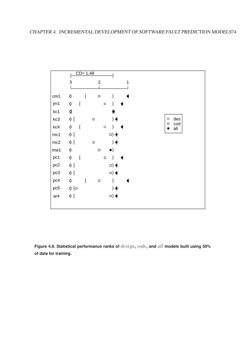
CHAPTER 4. INCREMENTAL DEVELOPMENT OF SOFTWARE FAULT PREDICTION MODELS74
CD= 1.48
123
cm1 ( )[ ]
jm1 ( )[ ]
kc1 ( )[ ]
kc3 ( )[ ]
kc4 ( )[ ]
mc1 ( )[ ]
mc2 ( )[ ]
mw1 ( )
pc1 ( )[ ]
pc2 ( )[ ]
pc3 ( )[ ]
pc4 ( )[ ]
pc5 ( )[ ]
ar4 ( )[ ]
descodall
Figure 4.9. Statistical performance ranks of design, code, and all models built using 50%
of data for training.

CHAPTER 4. INCREMENTAL DEVELOPMENT OF SOFTWARE FAULT PREDICTION MODELS75
two rank performance clusters (design and code vs. code and all). In almost half of themodels built from 10% data subsets, the performance of design, code, and all forms onerank performance cluster, i.e., their performance is statistically indistinguishable.
An interesting question arises regarding kc4 data set, in which design metrics outperformcode metrics. While all other projects use C, C++, or Java, kc4 relies on the scripting languagePerl. The use of Perl is an obvious project anomaly (in the context of the data sets includedin this dissertation) and a possible cause for much higher proportion of faulty modules in kc4
(48%). While we can not offer a more detailed analysis of the causes of anomalous manifes-tations in fault prediction models for this data set, we are inclined to suggest a more thoroughresearch consideration be given to software quality for projects which use scripting languagelike Perl.
4.2.3 Comparison of models developed using different classifiers
In the experiments reported so far, our results reflect median model performances achievedusing all five classification algorithms. As we mentioned before, by collapsing the performanceof all the classifiers and models into a single performance index (AUC), we intended to em-phasize the inherent properties of metrics data sets. In this section, we reveal the performanceimpact of different classification algorithms.
A recent study by Lessmann et al. [53] indicates that most classification algorithms do notoffer models which exhibit statistically significant performance differences. Sixteen out of 19algorithms included in Lessmann’s study belong to a “higher” rank cluster. In addition to the10 data sets included in their study,we use four additional project data sets: mc1, mc2, pc5, andar4. Out of five classifiers in our experiments, three (rf, log, and nb) were reported by Less-mann to achieve statistically indistinguishable performance. Further, Lessmann reports resultsonly from all metrics models using 2
3of the data for training. We find some very interesting
observations by experimenting with the three types of metric sets (design, code, and all) andby increasing the size of the training subset (10% to 90%). An additional difference betweenthe two studies reflects our opinion that software quality practitioners are most likely to useoff-the-shelf classifiers with their default parameter values. We follow this principle and report

CHAPTER 4. INCREMENTAL DEVELOPMENT OF SOFTWARE FAULT PREDICTION MODELS76
median results from 10-way cross validation. Lessmann et al. use grid-search approach to findan optimal combination of algorithmic hyper-parameters which maximize the performance ofeach classifier and report the mean values of AUC.
Our statistical hypotheses for this experiment can be formulated as follows:H30: Fault prediction models developed from the same data sets using five different classifica-tion algorithms do not result in statistically different performance.vs.H3α:At least two classifiers provide models with significantly different performance.
Figure 4.10 the outcome of out experiments analyzed through Demsar’s procedure. The 15
experiments (lines in Figure 4.10) reflect the three metrics groups and the five sizes of trainingsubsets. These results can be summarized as follows:
• Regardless of the classification algorithm, for all sizes of training subsets, models devel-oped from design metrics have significantly indistinguishable performance.
• For all sizes of training subsets, models developed from all metrics are grouped in twoperformance rank clusters; Random forest (rf) models are consistently in the higher rankcluster.
• Code metrics models fall in between. When trained on 10% to 50% of the data, theyresult in two rank clusters. When trained on larger subsets, all models fall into the singleperformance rank clusters.
These are very interesting insights. For all and code metrics models, we can infer that thechoice of classification algorithm in mature data sets (those where we train from larger subsets),consistent with Lessmann’s results, matters less than when the models are built early. When thesamples come earlier in the development life cycle from a smaller number of completed modules(10% or 25%), the choice of the classification algorithm matter more.
To gain better insights into these experiments, in Table 4.4, 4.5, and 4.6, we previewmedian and variance values of models developed for each group of metrics set: design, code,and all. The top median AUC for each project is marked in bold. We decided to report thesevalues from experiments in which models are trained using 50% of data as training subset.

CHAPTER 4. INCREMENTAL DEVELOPMENT OF SOFTWARE FAULT PREDICTION MODELS77
CD= 1.63
12345
a_10 )( [ ]
a_25 )( [ ]
a_50 )( [ ]
a_75 )( [ ]
a_90 )( [ ]
c_10 )( [ ]
c_25 )( [ ]
c_50 )( [ ]
c_75 )(
c_90 )(
d_10 )(
d_25 )(
d_50 )(
d_75 )(
d_90 )(
lognbbstbagrf
Figure 4.10. Comparison of 5 classification algorithms over different sizes of training subset
and three metric groups. Label “a 10” (or “d 50”), for example, stands for all (design)
metrics and 10%(50%) training subset. The reported results reflect performance ranks over
all 14 data sets.

CHAPTER 4. INCREMENTAL DEVELOPMENT OF SOFTWARE FAULT PREDICTION MODELS78
Table 4.4. Median and variance of AUC on design metrics of using 50% data as the training
subset
data bag bst log nb rfmedian var median var median var median var median var
cm1 0.59 0.0023 0.57 0.0026 0.57 0.0017 0.59 9e-04 0.54 0.0018jm1 0.67 0 0.67 0 0.68 0 0.63 4e-04 0.63 1e-04kc1 0.73 5e-04 0.74 4e-04 0.74 5e-04 0.74 3e-04 0.68 4e-04kc3 0.71 0.0167 0.73 0.0108 0.7 0.0151 0.79 0.004 0.74 0.0073kc4 0.79 0.0011 0.76 0.0018 0.77 0.002 0.79 9e-04 0.75 0.0017mc1 0.65 0.0067 0.6 0.0035 0.63 0.002 0.52 0.0034 0.74 0.0023mc2 0.65 0.0022 0.62 0.0029 0.59 0.0027 0.68 0.0027 0.62 0.0026mw1 0.76 0.0028 0.77 0.0019 0.75 0.0063 0.79 0.0016 0.71 0.0028pc1 0.68 0.0023 0.66 0.0012 0.62 0.0021 0.63 0.004 0.68 0.0024pc2 0.6 0.0091 0.71 0.0035 0.61 0.0202 0.79 0.0041 0.57 0.0094pc3 0.73 4e-04 0.72 3e-04 0.73 4e-04 0.68 0.0016 0.73 4e-04pc4 0.79 4e-04 0.79 3e-04 0.81 2e-04 0.75 0.0011 0.74 4e-04pc5 0.96 1e-04 0.96 0 0.94 1e-04 0.94 1e-04 0.95 1e-04ar4 0.7 0.01 0.68 0.0071 0.64 0.0108 0.76 0.0051 0.72 0.0041
Models built from 50% subsets are almost always statistically similar to those developed fromlarger and smaller training subsets.
From performance ranks in Figure 4.10, we find that random forest classifier achieves thehighest average rank for all and code metrics models. Of course, this does not mean thatrandom forest perform the best for each data set and training subset size. Table 4.5 and 4.6reveal almost half of code metrics models and a quarter of all metrics models feature a differentclassifier as the best one. This is not surprising and practitioners should be prepared to try outdifferent classification algorithms. Given that applying off-the-shelf classifiers with (mostly)default parameter values is not costly or difficult, the exercise may be worth the effort. However,looking back on Figure 4.10, in many cases, the differences will be at the margin of statisticalsignificance.

CHAPTER 4. INCREMENTAL DEVELOPMENT OF SOFTWARE FAULT PREDICTION MODELS79
Table 4.5. Median and variance of AUC on code metrics of using 50% data as the training
subset
data bag bst log nb rfmedian var median var median var median var median var
cm1 0.71 0.0018 0.66 0.0014 0.69 9e-04 0.67 0.0013 0.72 9e-04jm1 0.72 0 0.71 1e-04 0.71 0 0.69 0 0.72 0kc1 0.8 3e-04 0.79 3e-04 0.79 3e-04 0.79 2e-04 0.8 2e-04kc3 0.77 0.0037 0.76 0.0037 0.76 0.0071 0.82 0.0022 0.79 0.0014kc4 0.67 0.0021 0.66 0.0011 0.53 0.0026 0.55 0.0105 0.63 0.0039mc1 0.94 0.0046 0.95 1e-04 0.88 0.0017 0.8 0.0046 0.96 0.0012mc2 0.63 0.0038 0.64 0.0024 0.69 0.0046 0.69 0.0011 0.67 0.002mw1 0.78 0.0051 0.8 0.0022 0.75 0.0089 0.82 0.002 0.79 0.0024pc1 0.81 0.0017 0.79 0.0011 0.8 0.0015 0.7 0.0036 0.84 0.001pc2 0.73 0.0226 0.87 0.0064 0.72 0.0093 0.85 0.0044 0.81 0.007pc3 0.81 3e-04 0.81 3e-04 0.81 5e-04 0.78 5e-04 0.82 4e-04pc4 0.91 1e-04 0.91 1e-04 0.84 4e-04 0.77 0.0012 0.92 1e-04pc5 0.96 0 0.95 0 0.93 1e-04 0.93 0 0.97 0ar4 0.78 0.0079 0.82 0.0069 0.67 0.0087 0.81 0.0054 0.8 0.0052
Table 4.4, 4.5, and 4.6 also reveal that AUC indices across the five classifier models(within each row) are similar to each other. For example, in Table 4.6, all classifiers performvery well on pc5 data set and quite poorly on mc2 data set. It is evident that the performance ofa fault prediction model is determined more by the characteritics of a data set, rather than thedifferences between the classification algorithms. Similar variances represent further evidence.
It is also interesting to note that random forest classifier does not appear to rank well ondesign metrics models, although its results belong to the same rank cluster with the other fouralgorithms. The number of attributes representing design metrics is lower than the numberof attributes in code and especially, all models. It is known that the strength of random forestclassifier are the data sets with a large number of attributes and a large number of instances [14].

CHAPTER 4. INCREMENTAL DEVELOPMENT OF SOFTWARE FAULT PREDICTION MODELS80
Table 4.6. Median and variance of AUC on all metrics of using 50% data as the training
subset
data bag bst log nb rfmedian var median var median var median var median var
cm1 0.73 0.001 0.71 0.0019 0.70 0.0024 0.70 0.0011 0.76 8e-04jm1 0.73 0 0.71 1e-04 0.71 0 0.69 0 0.74 0kc1 0.8 1e-04 0.79 3e-04 0.79 2e-04 0.79 1e-04 0.81 1e-04kc3 0.72 0.0052 0.76 0.0027 0.53 0.0166 0.80 0.0023 0.78 0.0015kc4 0.82 0.0014 0.80 0.0024 0.81 0.0036 0.78 0.0025 0.82 0.0014mc1 0.96 0.0048 0.95 2e-04 0.94 0.0039 0.80 0.0019 0.98 8e-04mc2 0.67 0.0032 0.65 0.0047 0.64 0.0049 0.72 0.0014 0.70 0.0031mw1 0.77 0.0048 0.79 0.0047 0.72 0.0063 0.82 0.0019 0.79 0.003pc1 0.82 0.0013 0.80 9e-04 0.76 0.0047 0.77 7e-04 0.85 5e-04pc2 0.74 0.0347 0.85 0.0048 0.65 0.0185 0.87 0.004 0.83 0.0071pc3 0.81 3e-04 0.81 3e-04 0.82 7e-04 0.78 0.0017 0.83 3e-04pc4 0.92 2e-04 0.92 1e-04 0.90 3e-04 0.84 3e-04 0.94 1e-04pc5 0.97 0 0.96 0 0.95 1e-04 0.94 0 0.97 0ar4 0.78 0.0036 0.84 0.0058 0.68 0.0067 0.80 0.0054 0.81 0.0035
4.3 Discussion
The experiments reported in this chapter have been motivated by the hypothesis that com-bining software metrics from different stages in the development benefits the accuracy of faultprediction models. This motivation includes the utilization of different metrics types, thoseavailable from software design or code, as well as the proactive use of measurements fromsoftware modules for the development of fault prediction models when they become availableduring project development. Publicly available NASA MDP and Promise repositories offer asubstantial number of data sets, 14 of which we have used in the experiments. The large numberof project data sets and a rigorous statistical test procedures we applied offer strong evidence insupport of our conclusions, presented below.

CHAPTER 4. INCREMENTAL DEVELOPMENT OF SOFTWARE FAULT PREDICTION MODELS81
The starting position for our analysis of the relative strengths of design and code metricsin building fault prediction models comes from Zhao et al. [91]. They claimed that design andcode models perform comparatively well and that little improvement can be achieved if designand code metrics are jointly used in fault prediction. Our results from 14 data sets of NASAMDP show that although there is no significant statistical difference between design and codemetrics, but the combination of design and code metrics usually outperform design metricsstatistically. However, given the early available of design metrics,
The impact the size of the fault data set used for training has on model performance isalso significant and interesting. One of the basic questions regarding the practicality of faultprediction is: When does the project have sufficient amount of data to build a model? Beforewe describe our recommendations, it is necessary to mention that in many organizations faultinformation from early (or earlier) product releases has been successfully used for fault predic-tion for the new release [71,82]. In organizations which practice software product lines or thosewhere upgrades form the majority of project releases, data sufficiency is not a major problem.But there are many other organizations and projects which develop oneof- a-kind systems. Thir-teen out of 14 data sets we analyzed come from such environments. These organizations mustrely on the metrics from reused modules and those delivered and tested early in the developmentlife cycle for building fault prediction models.
We believe the results reported here have been obtained following a valid experimentalmethodology, using publicly available data sets. As any other experimental study we are awareof potential validity threats too. For example, we mentioned that the design metrics used inthe experiments have been reengineered from the code. While in principle similar metrics can(and have been) extracted from design documentation, it is likely that the metrics used in ourexperiments reflect the code more faithfully than the metrics collected at the design stage would.Had design models demonstrated better fault prediction performance than code models, onecould argue that any reduction in the code-level details from attributes would have a tendencyto improve performance. But, design models in our experiments do not perform as well as codemodels. Therefore, it seems logical that if design metrics do not reflect code structure as closeas they do in our data sets, this would likely deteriorate the performance even further. Withoutadditional research, we cannot offer further assurances.
It is also worth repeating here that the data sets we analyzed do not contain information

CHAPTER 4. INCREMENTAL DEVELOPMENT OF SOFTWARE FAULT PREDICTION MODELS82
about when in the project development life time modules became available. To advocate in-cremental model development, we made the assumption that random selection of data subsetused for training (repeated 10 times in each experiment) represents a valid sample of modulesas if they became available before the modules we used for model evaluation. We are awarethat software modules that become available early might suffer from quality deficiencies whichprojects reduce as their processes mature. If fault introduction is reduced over the life time ofthe project, our results about the suitability of fault prediction models built from smaller datasubsets may be overly optimistic. Also, this might imply that updating models more frequentlyduring the projects life time is warranted. Unfortunately, the data sets we use do not allow us tostudy this problem further.
Lastly, we did not investigate the impact of feature selection on model performance. Featureselection algorithms minimize the number of attributes used in model development based onsome measure of their information content. Our experience with MDP datasets indicates thata smaller number of attributes (metrics), typically a dozen or less, could offer models thatperform almost as well as the models which use the entire set of attributes [62]. This couldhave an impact on the effort invested in metrics collection. But, we have never been able todevelop a model from a reduced set of attributes which outperforms models developed fromcomprehensive attribute sets. For this reason, we believe that feature selection is not likely toimpact the validity of our results.
4.4 Summary
Our results confirm that the performance of design and code models, measured through thearea under the ROC curve (AUC), is typically statistically indistinguishable. In other words,although code metrics based models outperform design metrics models, the performance mar-gin is not statistically significant. On the other hand, the performance of models built fromall metrics (which include design and code metrics) typically outperform design models by astatistically significant margin. Our experiments, therefore, offer support for utilizing a com-bination of design and code metrics in building fault prediction models. However, if designmetrics are available earlier, design models should not be discarded as they offer meaningfulfault prediction performance.

CHAPTER 4. INCREMENTAL DEVELOPMENT OF SOFTWARE FAULT PREDICTION MODELS83
Most results from our experiments which test the impact of the training data size on thefault prediction performance are not surprising. When derived from a larger data set, modelperformance improves. The interesting aspect of our results comes from statistical hypothesistesting. In simple terms, the performance margin between models derived from 50% data sub-sets and those derived from just 10% is not statistically significant. Further, models built from50% data subsets and 90% data subsets typically belong the the same performance cluster too(but models built from 10% and 90% do not). The implication of this result is, we believe, verypositive. Models developed from data sets, presumably early in the project life time, offer faultprediction capability comparable with models that can only be developed much later. There-fore, while updating the fault prediction model is a good idea, it does not have to be practicedoften. This conclusion offers the real chance to optimize the cost of fault prediction modeldevelopment. Fault prediction models, in turn, optimize the cost of verification and validationactivities.
We believe the results from both experiments support the general hypothesis: fault detectorscan be improved by increasing the information content of the training set. Therefore continuingto explore the effects of combining the attributes from multiple phases of the developmentlife cycle, process and business related attributes, appears to be the most promising researchdirection [40, 69, 85].
In the third group of experiments, we examined the impact of the selection of the classifica-tion algorithm in fault prediction modeling. In the recent paper, Lessmann [53] offers convinc-ing arguments that most classification algorithms offer statistically the same performance (i.e.,their performance differences are not significant). One limitation of Lessmann’s analysis is theuniform use of 2
3of the data for model training. In our experiments we varied the size of the
training subset and the type of metrics used for training. We observed that statistically signif-icant differences between classification algorithms do occur when models are developed fromsmaller training subsets. Further, significant differences are more likely to occur when trainingfrom all and code metrics than from design metrics. Consequently, we recommend experimen-tation with several classification algorithms, recommended in the literature (for example [53])for fault prediction modeling.
Combined, the outcomes of our experiments provide a good guidance for an incrementalprocess for software fault prediction modeling. Models can be built early, from design metrics

CHAPTER 4. INCREMENTAL DEVELOPMENT OF SOFTWARE FAULT PREDICTION MODELS84
and/or from relatively small subsets of available data. Updating such early models is recom-mended. The frequency of such updates can be optimized as model performance gains justifyintermittent (sporadic) upgrades, rather than recurring ones.
We conclude this chapter by submitting our findings with the questions posed in the disser-tation:
• Q2: Are design metrics good enough to be fault-proneness predictors?Answer: Yes. Design metrics are useful fault-prone predictors.
• Q3: Are code metrics good fault-prone predictors?Answer: Yes.
• Q4: Do fault prediction models built from a combination of requirement, design, andcode metrics provide better performance than models built from any metrics subset?Answer: The performance of the combination models is usually better than design orcode metrics alone.
• Q5: How large is a training subset needed for building meaningful fault prediction mod-els?Answer: 10% subset data can be used to train models, this allow software fault predictionearly in the project life cycle.
• Q6: How large is a training subset needed in order to achieve the best performance faultprediction models?Answer: Using 50% data as training subset will achieve the best performance modelsstatistically.

Chapter 5
Cost-specific Fault Prediction Models
This chapter will investigate the following problems:
• Q7: How can we incorporate different misclassification costs into fault prediction mod-els?
• Q8: How can we achieve the lowest misclassification cost for a given data set?• Q9: How can fault prediction models guide different risk level projects from misclassifi-
cation cost perspective?• Q10: How can we evaluate individual module’s specific misclassification cost in fault
prediction models?
In this chapter, we first introduce the cost curve, a novel evaluation technique to evaluatefault prediction models. With the introduction of cost curves, we are able to answer Q7 and Q8.Then, we will tackle problems Q9 and Q10 through the experiments. Finally, we will discussour results.
5.1 Cost Models
While the techniques for model development which explicitly account for misclassificationcost differential have not been studied in software fault prediction modeling, there have been
85

CHAPTER 5. COST-SPECIFIC FAULT PREDICTION MODELS 86
attempts to include cost factors into model evaluation. F-measure, for example, offers a tech-nique to account for the cost factor [39] when comparing different models. Khoshgoftaar andAllen [49] proposed the use of prior probabilities of misclassification to select classifiers whichoffer the most appropriate performance. In [50] they compare the return-on-investment in alarge legacy telecommunication system when V &V activities are applied to software modulesselected by a quality model vs. at random. Cost has been considered in test case selection forregression testing too [28].
There is a steady trend in fault prediction modeling literature recommending model evalu-ation with lift charts [39], sometimes called Alberg diagrams [72, 74]. Lift is a measure of theeffectiveness of a classifier in the detection faulty modules. It calculates the ratio of correctlyidentified faulty modules with and without the predictive model. Lift chart is especially usefulwhen the project has resources to apply verification activities to a limited number of modules.Cost effectiveness measure described by Arisholm et al. [7] can account for the nonuniformcost of module-level V &V .
5.1.1 Cost Curve
Cost curve, proposed by Drummond and Holte [26], is a visual tool that allows us to de-scribe classifier’s performance based on the cost of misclassification. The x-axis representsprobability cost function, denoted PC(+). Its y-axis represents normalized expected misclas-sification cost. It indicates the difference between the maximum and the minimum cost ofmisclassifying faulty modules.
Let us denote the faulty module with a “+” and a fault-free module as “-”. C(+|−) denotesthe cost of incorrectly predicting a fault-free module as faulty. C(−|+) represents the cost ofmisclassifying a faulty module as being fault-free. p(+) and p(-) are the probabilities of a soft-ware module being faulty or fault free when the project is deployed. Because we are uncertainabout the value of p(+) and p(-), thus, we plot all kinds of possible values of p(+) (implicitlyp(-)) in cost curve. These probabilities can become known only after the deployment of themodel, since the proportion of faulty modules in model’s training and test sets are approxima-tions of the proportion of faulty modules the model will encounter during its field use. Costcurves support visualization of model’s performance across all possible values of p(+) and p(-),

CHAPTER 5. COST-SPECIFIC FAULT PREDICTION MODELS 87
offering performance predictions for various deployment environments. Equations 5.1 and 5.2present the formulae for computing the values that appear on x-axis and y-axis:
x− axis =p(+) ∗ C(−|+)
p(+) ∗ C(−|+) + p(−) ∗ C(+|−)(5.1)
y − axis = (1− PD − PF ) ∗ PC(+) + PF (5.2)
Typical regions of a cost curve are shown on Figure 5.1. The diagonal line connectingpoint (0,0) to (1,1) stands for a trivial classifier(TC) that always classifies all the modules tofault-free. And the points in the area above this line indicate the performance of a classifier isworse than the trivial classifier. The other diagonal line, connecting point (0,1) to (1,0), standsfor another trivial classifier that always classifies all the modules as faulty modules. And thepoints above this line are cases where the performance of a classifier is worse than this trivialclassifier. The horizontal line connecting point (0,1) to (1,1) stands for the extreme situationwhen the model misclassifies all the modules. The x-axis line represents for the ideal modelthat correctly classifies all the modules. From this typical cost curve, we find that to draw they-axis in the range of 0 to 0.5 is enough as the lower half of the curve is the most interestingpart because we are not interested in a classifier which perform worse than trivial classifier. Asthe figures we present in the following, we restrict y-axis from 0 to 0.5.
An ROC curve connects a set of calculated (PF, PD) pairs. Cost curves are generated bydrawing a straight line connecting points (0,PF) to (1,1-PD), corresponding to (PF, PD) pointin the ROC curve. After drawing all straight lines that have the counterpart points in the ROCcurve, the lower envelope of cost curve is formed by connecting all the intersection points fromleft to right. Figure 5.2 shows an example of a cost curve resulting from the application ofLogistic classification model in project KC4. The lower envelope of the cost curve correspondsto the convex hull in the ROC curve. ROC curves and cost curves are closely related: a point inthe ROC curve corresponds to a line in the cost curve.

CHAPTER 5. COST-SPECIFIC FAULT PREDICTION MODELS 88
Figure 5.1. Typical regions in cost curve.
0.5
0.45
0.4
0.35
0.3
0.25
0.2
0.15
0.1
0.05
0.0
1.00.90.80.70.60.50.40.30.20.10.0
Probability Cost
Norm
aliz
ed E
xpec
ted C
ost
Logistic on KC4
Figure 5.2. A cost curve of logistic classifier on KC4 project data.

CHAPTER 5. COST-SPECIFIC FAULT PREDICTION MODELS 89
The Meaning of Classification Result
Assume the ratio of misclassifying a fault-free module to that of misclassifying a faulty moduleis ϕ, that is, ϕ = C(+|−):C(−|+). Equation 5.1 can be rewritten in term of ϕ as:
x− axis = PC(+) =p(+)
p(+) + p(−) ∗ ϕ(5.3)
In Equation 5.3, p(+) is the percentage of faulty module in the project, and p(-) = 1- p(+).Thus, if we are interested in a particular value of ϕ, we can calculate the corresponding PC(+)value easily according to Equation 5.3. In the mean time, if we know PC(+) value, the cor-responding ϕ can be derived directly. For instance, say, in KC4 data, from Table 2.3, wecan see that the proportion of faulty modules in KC4 is 48%. Therefore, p(+) = 0.48 andp(−) = 1 − 0.48 = 0.52. (1) In the case of ϕ = 1, that is, the cost of misclassifyinga faulty module and the cost of misclassifying a fault-free module are the same, C(+|−) =C(−|+), according to Equation 5.3, we get that PC(+) = 0.48. (2) In the case of ϕ = 5,that is, the misclassification of a fault-free module cost 5 times more than that of the misclas-sification of a faulty one, we have C(+|−) : C(−|+) = 5. Taking this to Equation 5.3, wehave PC(+) = 0.156. (3) In the case of ϕ = 1
5, that is, C(+|−) : C(−|+) = 1
5, we have
PC(+) = 0.82.
Figure 5.3 shows cost curves of 5 classifiers (bagging, boosting, logistic, naiveBayes, andrandom forest) on KC4 data. The places where ϕ = 100, 5, 1
5, 1
100are indicated by vertical
dashed lines of corresponding points at 0.009, 0.156, 0.82, and 0.99 respectively. If we are inter-ested in a particular point (or a particular misclassification ratio),i.e., PC(+) = 0.48 (ϕ = 1),we should choose a classifier that offers the minimal misclassification cost along the corre-sponding vertical line (PC(+) = 0.48). From Figure 5.3,we can see that when PC(+) = 0.48,the best model which has the minimal misclassification cost is boosting. When PC(+) < 0.48,the misclassification cost of fault-free modules is greater than that of misclassifying a faultymodule (ϕ > 1). The region PC(+) < 0.48 stands for models which are adequate for “cost-adverse” projects in software engineering. The cost region of PC(+) > 0.48 represents modelswhich are adequate for “risk adverse” projects, those where misclassifying a faulty module issignificantly more consequential (0 < ϕ < 1). Cost curves open significant opportunities forcost-based software quality management. Misclassification costs can dictate the preference for

CHAPTER 5. COST-SPECIFIC FAULT PREDICTION MODELS 90
the model and model parameters which are the most appropriate for the given project.
0.5
0.45
0.4
0.35
0.3
0.25
0.2
0.15
0.1
0.05
0.0
1.00.90.80.70.60.50.40.30.20.10.0
Probability Cost
Norm
aliz
ed E
xpec
ted C
ost
bag
bst
log
nb
rf
KC4
1
100
5
1/5
1/100
Figure 5.3. Cost curve of 5 classifier on KC4.
The goal of cost curve is to minimize the misclassification cost, that is, minimize the lowerenvelope area. The smaller the area under the lower envelope boundary is, the lower the mis-classification cost would be and, hence, the better the performance of the classifier. However, itis likely that a single model will not be equally good in all cost regions. If a project evolves toan understanding that the misclassification cost differential is not the same one used in the past,the project may decide to change the quality model it uses even though the underlying metricdistributions in the dataset remain the same. Cost curves support this type of decisions. Forinstance, looking back to Figure 5.3, in the interval (0.22, 0.385), random forest has the bestperformance; in the interval (0.385,0.88), boosting outperforms the other learners; finally,in therange from 0.88 close to 1.0, logistic model turns out to have the minimal misclassification.
In Figure 5.3, when PC(+) is from 0 to 0.2, bagging and boosting perform worse than trivialclassifier which simply classifies every module as faulty-free. When PC(+) is from 0 to 0.05, the

CHAPTER 5. COST-SPECIFIC FAULT PREDICTION MODELS 91
other three learners logistic, naiveBayes, and random forest overlap with the trivial classifier,it means their performance are similar to that of the trivial classifier. Let’s look at the otherend where PC(+) close to 1. After PC(+) > 0.87, naiveBayes performs worse than the trivialclassifier which classifies each module as faulty one. After PC(+) > 0.95, bagging overlapswith the trivial classifier too. We can see that at the both ends of x-axis where PC(+) is eitherclose to 0 or 1, the trivial classifier is not a bad classifier with allowable performance. Whichmay means in some extreme situations, extreme cost adverse project and risk adverse project,the V&V activity of check nothing (extreme cost adverse) and check everything (extreme riskadverse) would be meaningful.
Cost curves have the ability to reveal the differences among classifiers from perspectivesthat are not obvious in other commonly used curves such as Receiver Operating Characteristic(ROC). Figure 5.4 demonstrates their differences using MC2 dataset as an example. The costcurve, shown in panel (b) of Figure 5.4 provides a clear answer to the comparison of two clas-sifiers: Logistic classifier is better than random forest (rf) because its lower envelope is alwaysbelow that of random forest. Deriving this conclusion from ROC curves would be difficult.
Figure 5.4. (a) A ROC curve (b) Corresponding cost curve of MC2.

CHAPTER 5. COST-SPECIFIC FAULT PREDICTION MODELS 92
Statistical Significance in Cost Curve
The measure of classifier’s performance is derived from a confusion matrix. In cost curve, aswell as in other performance analysis graphs, a confidence interval is generated from a seriesof confusion matrices. We illustrate the use of confidence bounds on cost curves, following theprocedure outlined by Drummond and Holte in [26]. The procedure is based on the resamplingof typically 500 confusion matrices using the bootstrap method. The 95% confidence intervalfor a specific PC(+) value, for example, is obtained by eliminating the highest and the lowest2.5% of the normalized expected cost values.
In some ranges of the curve, the performance between two classifiers may have significantdifference, but in the other ranges, it may not. Figure 5.5 shows an example of the difference inperformance between two classifiers, IB1 and j48 on PC1 dataset. The shaded area in Figure 5.5represents the 95% confidence interval. There are three lines inside the shaded area. The middleline in the shaded area represents the difference between the means of the two classifiers IB1 andj48. The other two lines along the edges of shaded area represent the 95% confidence interval ofthe difference between the mean of two classifiers. If the confidence interval contains zero line,then there is no significant difference between the two classifiers; Otherwise, there is. The largerthe distance of the confidence interval from the zero line, the more significant the differencebetween the two classifiers. Referring to Figure 5.5, when PC(+) is in the range of (0.0, 0.1),the confidence interval is above the zero, indicating IB1 outperforms j48. In the range (0.27,0.59), the confidence interval is below the zero line, indicating that j48 performs better than IB1.Between (0.1, 0.27) and (0.59, 0.64), the confidence interval contains the zero line indicatingno significant difference between the two classifiers. When PC(+) > 0.64, the performanceof the two classifiers is the same. Given that the proportion of faulty modules in project PC1is 7%, at PC(+) = 0.07 the misclassification costs for faulty and fault-free classes is thesame, C(+|−) = C(−|+). When PC(+) < 0.07 the misclassification of fault free modulesoutweighs the misclassification of faulty modules. The opposite is true for 0.07 < PC(+).Cost curve analysis shows that (1) j48 is a bad choice when PC(+) < 0.07 (worse even thanthe trivial classifier); (2) j48 outperforms IB1 in (0.27, 0.59) region; (3) in other regions of thecost curve, IB1 and j48 perform similarly.
The confidence band in cost curve reveals aspects which cannot be inferred from the sta-

CHAPTER 5. COST-SPECIFIC FAULT PREDICTION MODELS 93
tistical analysis of AUC in ROC curves. When misclassification costs are known or can beguessed, cost curves and their statistical analysis provide the most meaningful guidance formodel selection.
Figure 5.5. The 95% cost curve confidence interval comparing IB1 and j48 on PC1 dataset.
5.2 Experimental Design
Given the problems stated in the dissertation, we carried out our experiments in the follow-ing steps.
• Compare the “best” performance classifier to the trivial classifier (TC) to justify the ben-efit of using software fault prediction models.
• Compare the “best” and the “worst” performance classifiers for those “worst” classifiersare not worse than the trivial classifier (TC).
• Investigate which classifier will generate the lowest misclassification cost for a modulewith specific risk level.
In these experiments, we used the five classifiers: random forest(rf ), boosting(bst), logistic(log),naiveBayes(nb), and bagging(bag), and all 16 data sets from the NASA MDP repository [2] and

CHAPTER 5. COST-SPECIFIC FAULT PREDICTION MODELS 94
PROMISE (3 datasets) [13] which are shown in Table 2.3.
5.3 Comparison of the “Best” Classifier Against the Trivial Classifier
In practice, it is difficult to determine the exact value of misclassification ratio ϕ = C(+|−) :
C(−|+). But it should not be difficult to estimate project’s approximate risk level in terms ofa range of probability misclassification costs. For this chapter, we divide projects into threegroups based on their misclassification risk levels. We discussed this simplistic grouping withdevelopers involved in projects we analyze and they found it reasonable. A project exhibits alow risk level if its misclassification ratio ϕ = C(+|−) : C(−|+) is in range of (100,5). Insimple terms, misclassifying a fault free module as fault module is highly undesirable, 5 to 100times more than misclassifying a faulty modules as fault free. These are clearly cost adverseprojects, trying to optimize V &V activity and speed up product delivery. A project is assigneda high risk level if the ultimate goal of analysis is to identify as many fault prone modules aspossible. Such risk averse projects typically allocate a substantial portion of their budgets toverification activities. Their range of misclassification cost ratio ϕ = C(+|−) : C(−|+) is(1
5, 1
100). Medium risk projects are the remaining ones, for which the misclassification cost
ratio ϕ is in the interval (5, 15).
The risk levels for 16 data sets used here have been determined in discussion with softwarequality engineers at NASA, and the metrics collection experts at the white goods manufacturershown in Table 5.1. Seven NASA control and navigation software projects are categorized ashaving high risk level. The three data sets from the white-goods manufacturer are classified aslow risk, mostly due to strong time-to-market pressures. Two additional NASA data sets, KC4and MC2, are also assigned a low risk level: KC4 is a ground-based subscription server andMC2 is a video guidance system. The remaining four projects are assigned medium risk level.These data sets are associated with storage management for ground data, a zero gravity exper-iment, and a spacecraft instrument system. The misclassification cost ratio (ϕ) are assignedaccordingly. Since we know the ground truth about fault prone modules in all data sets, assign-ing probability parameters p(+) and p(−) for our experiments is simple. From Equation 5.3, weobtain probability costs PC(+) and calculate the range of interest for each project, implied byits risk classification and probability parameters. Specific values of these parameters are shown

CHAPTER 5. COST-SPECIFIC FAULT PREDICTION MODELS 95
in Table 5.1.
5.3.1 Analysis
Having determined risk levels for all the projects in the above section, we want to under-stand the impact of cost curve modeling in evaluating fault prediction models. More precisely,we want to know how well the models perform when misclassification cost is taken into ac-count. Can cost modeling be used to argue for or against software fault prediction modeling inthe context of a specific project?
We developed cost curves describing the performance of fault prediction models from thefive classifiers on each of the 16 data sets listed in Table 2.3. Figure 5.6 shows 15 cost curvesexcept KC4 (KC4 is shown as an example in Figure 5.3). To increase readability of thesediagrams, we limit the displayed range of the probability cost (x-axis) to include only the regionof interest inferred from the project’s risk level: Low–(100, 5); medium–(5, 1
5); or high –
(15, 1
100). The lower and upper bound of each region are marked with thin solid vertical lines.
Most cost curves also show the operational point where ϕ = C(+|−) = C(−|+) = 1.
A quick look at the curves in Figure 5.6 reveals two general trends: (1) when PC(+) isclose to 0 or close to 1, the performance of fault prediction models becomes very similar totrivial classifiers; (2) the most significant performance benefit of fault prediction modeling isusually achieved in the middle region of the cost curve, surrounding PC(+) = 0.5. Thisobservations imply that fault prediction modeling has limited impact in cases of extremely riskaverse or cost averse projects. On the extreme risk averse side, we would like the model to iden-tify all the faulty modules. On the extreme cost averse side, we do not want to misclassify anyfault free module as fault prone. These goals are, in fact, achieved by the two trivial classifierswhich assign all the modules in a single class! In binary classification problems, near perfectmodule assignment to one class results in high misclassification rate in the other class. Highmisclassification cost differential between the two classes, therefore, leads to trivial solutions.
Table 5.1 shows each project’s risk level, the corresponding probability cost range of inter-est and the classification algorithm that achieves the best performance inside the probability costrange. The table also shows the probability cost range in which the best model is significantly
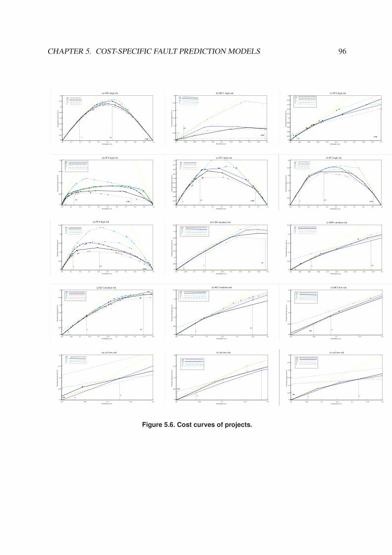
CHAPTER 5. COST-SPECIFIC FAULT PREDICTION MODELS 96
0.4
0.35
0.3
0.25
0.2
0.15
0.1
0.05
0.0
1.00.90.80.70.60.50.40.30.20.10.0
Probability Cost
Norm
aliz
ed E
xpec
ted C
ost
bagbstlognbrf
(a) JM1-high risk
1 1/51/100
0.3
0.25
0.2
0.15
0.1
0.05
0.0
0.40.360.320.280.240.20.160.120.080.040.0
Probability Cost
No
rmal
ized
Ex
pec
ted
Co
st
bagbstlognbrf
(b) MC1- high risk
1
1/5
1/100
0.2
0.18
0.16
0.14
0.12
0.1
0.08
0.06
0.04
0.02
0.0
0.30.270.240.210.180.150.120.090.060.030.0
Probability Cost
Norm
aliz
ed E
xpec
ted C
ost
bagbstlognbrf
(c) PC2-high risk
1
1/51/100
0.2
0.15
0.1
0.05
0.0
1.00.90.80.70.60.50.40.30.20.10.0
Probability Cost
No
rmal
ized
Ex
pec
ted
Co
st
bagbstlognbrf
(d) PC5-high risk
1
1/51/100
0.3
0.27
0.24
0.21
0.18
0.15
0.12
0.09
0.06
0.03
0.0
1.00.90.80.70.60.50.40.30.20.10.0
Probability Cost
Norm
aliz
ed E
xpec
ted C
ost
bagbstlognbrf
(e) PC1-high risk
11/5 1/100
0.3
0.25
0.2
0.15
0.1
0.05
0.0
1.00.90.80.70.60.50.40.30.20.10.0
Probability Cost
No
rmal
ized
Ex
pec
ted
Co
st
bagbstlognbrf
(f) PC3-high risk
11/5
1/100
0.25
0.2
0.15
0.1
0.05
0.0
1.00.90.80.70.60.50.40.30.20.10.0
Probability Cost
Norm
aliz
ed E
xpec
ted C
ost
bagbstlognbrf
(g) PC4-high risk
1 1/5
1/100
0.35
0.3
0.25
0.2
0.15
0.1
0.05
0.0
0.50.450.40.350.30.250.20.150.10.050.0
Probability Cost
Norm
aliz
ed E
xpec
ted C
ost
bagbstlognbrf
(h) CM1-medium risk
1
5
1/5
0.25
0.2
0.15
0.1
0.05
0.0
0.30.270.240.210.180.150.120.090.060.030.0
Probability Cost
No
rmal
ized
Ex
pec
ted
Co
st
bagbstlognbrf
(i) MW1-medium risk
1
5
1/5
0.3
0.25
0.2
0.15
0.1
0.05
0.0
0.50.450.40.350.30.250.20.150.10.050.0
Probability Cost
No
rmal
ized
Ex
pec
ted
Co
st
bagbstlognbrf
(j) KC1-medium risk
1/515
0.25
0.2
0.15
0.1
0.05
0.0
0.30.250.20.150.10.050.0
Probability Cost
Norm
aliz
ed E
xpec
ted C
ost
bagbstlognbrf
(k) KC3-medium risk
1
5
1/5
0.2
0.15
0.1
0.05
0.0
0.20.150.10.050.0
Probability Cost
No
rmal
ized
Ex
pec
ted
Co
st
bagbstlognbrf
(l) MC2-low risk
1005
0.2
0.15
0.1
0.05
0.0
0.20.150.10.050.0
Probability Cost
Norm
aliz
ed E
xpec
ted C
ost
bagbstlognbrf
(m) ar3-low risk
100 51
0.2
0.15
0.1
0.05
0.0
0.20.150.10.050.0
Probability Cost
No
rmal
ized
Ex
pec
ted
Co
st
bagbstlognbrf
(n) ar4-low risk
100
5
0.3
0.25
0.2
0.15
0.1
0.05
0.0
0.30.250.20.150.10.050.0
Probability Cost
Norm
aliz
ed E
xpec
ted C
ost
bagbstlognbrf
(o) ar5-low risk
1005 1
Figure 5.6. Cost curves of projects.

CHAPTER 5. COST-SPECIFIC FAULT PREDICTION MODELS 97
Table 5.1. Probability cost of interested and significant ranges.Data risk probability cost best significant range and significant
range of interested classifier % significantRangeinterestedRange ϕ range
JM1 high (0.545, 0.960) rf (0.545, 0.72) 42.17% (15 , 1
10 )
MC1 high (0.031, 0.391) rf entire 100% (15 , 1
100 )
PC2 high (0.021, 0.297) rf (0.15, 0.297) 53.26% ( 140 , 1
100 )
PC5 high (0.134, 0.756) rf entire 100% (15 , 1
100 )
PC1 high (0.261, 0.876) rf (0.261, 0.80) 87.64% (15 , 1
50 )
PC3 high (0.368, 0.921) rf (0.368, 0.82) 81.74% (15 , 1
40 )
PC4 high (0.411, 0.933) rf entire 100% (15 , 1
100 )
CM1 med. (0.037, 0.489) rf (0.11, 0.489) 83.85% (1.5, 15 )
MW1 med. (0.014, 0.264) bst (0.13, 0.264) 53.6% (12 , 1
5 )
KC1 med. (0.031, 0.447) rf (0.14, 0.447) 73.8% (1, 15 )
KC3 med. (0.013, 0.252) bag(nb) (0.18, 0.252) 30.13% ( 13.3 , 1
5 )
KC4 low (0.009, 0.156) nb (0.10, 0.156) 38.10% (8, 5)
MC2 low (0.005, 0.087) rf,log no 0
ar3 low (0.001, 0.028) bst no 0
ar4 low (0.002, 0.044) bst no 0
ar5 low (0.003, 0.054) bst no 0

CHAPTER 5. COST-SPECIFIC FAULT PREDICTION MODELS 98
better (using the 95% confidence interval) than the trivial classification, the size of statisticallysignificant interval with respect to the probability cost range of interest and the correspondingrange of misclassification cost ratio ϕ in which the model outperforms the trivial classification.The last column offers the project-specific misclassification cost interval in which software faultprediction models offer benefits. If the project’s actual misclassification cost ratio is not withinthis interval, using models to select fault prone modules would not justify the effort.
From these experiments, it became obvious that we need to understand whether fault pre-diction models are any better than the trivial classifier within specific misclassification costranges. For this purpose, we applied a rigorous statistical significance analysis procedure. Thisanalysis indicates that although nb, boosting and bagging outperform other algorithms for lowand medium risk projects, their classification results are in many cases not significantly betterthan the trivial classification. The most benefit we can achieve is in high risk projects wheremost classifiers have better performance than the trivial classifier.
The data sets described as high risk were derived from mission and safety critical devel-opment projects. Figures 5.6 (a)-(g) depict the cost curves of high risk projects. Althoughwe noted that highly imbalanced misclassification cost may favor the trivial classification, thehigh risk data sets we analyzed all indicate that fault prediction models outperform the triv-ial classifiers. However, statistical significance does not necessarily span over the entire rangeof the misclassification cost ratio (1
5, 1
100). For example, for JM1 in Figure 5.6(a), the model
generated using random forest algorithm performs significantly better than the trivial classifierin the probability cost region (0.545, 0.72), which corresponds to the misclassification costratio range ϕ = (1
5, 1
10). Similar observations can be made for projects PC1 and PC3: when
PC(+) < 0.80(ϕ ' 150
) or PC(+) < 0.82 (ϕ ' 140
), respectively, best models perform bet-ter than the trivial classifier. The same is not true for higher misclassification cost ratios, ϕ > 1
50
or ϕ > 140
, respectively. In PC2 data set, the statistically significant performance differencebetween the best classifier and the trivial classifier lays in the region of the highest misclassifica-tion cost ratio, ϕ = ( 1
40, 1
100). With the remaining three high risk projects, MC1, PC4 and PC5,
the best model outperforms the trivial classifier in the entire range of misclassification cost ratio.It is also interesting to observe that in all high risk projects, models developed using randomforest algorithm outperform other machine learning algorithms used in our experiments.
The cost curves of medium risk projects CM1, MW1, KC1, and KC3, where ϕ = (5, 15),

CHAPTER 5. COST-SPECIFIC FAULT PREDICTION MODELS 99
are shown in Figures 5.6(h)-(k). Interestingly, fault prediction models do not outperform trivialclassification throughout the range of interest. Cost curve diagrams indicate that medium riskresides in the low range of the probability cost, i.e., PC(+) < 0.5. This is not a region of themost beneficial performance impact. Bagging, boosting and random forest are the classificationalgorithms which seem to perform the best for medium risk projects.
The cost curves of low risk projects MC2, ar3, ar4 and ar5 are depicted in Figures 5.6(l)-(o) while KC4 is shown in Figure 5.3. In these projects, the trivial classification is as good forselecting fault prone modules as any of the models we experimented with. In other words, ifthe goal of software quality modeling is to avoid wasting tight V &V budgets on verification offault-free modules, the best way to achieve this is by not classifying any module as fault prone.
Explaining this observation is not difficult. In most projects the proportion of fault pronemodules is small, causing a severe class size imbalance between faulty and fault-free modules.For example, in MC1, only 0.64% of the modules are fault prone and 99.36% are fault free. Inour study, KC4 has a large percentage of faulty modules, 48%, but it is also the smallest project(only 125 modules) and the only one that uses a scripting language (Perl). In MC1, identifying61 faulty amongst 9, 644 modules is a difficult task for any classification algorithm. What makesthe effort worthy is the high cost premium for fault detection. If the premium is not there, givenwhat we know about this data set, no fault prediction model justifies the investment. Lookingat the shape of cost curves, the most significant benefits for software assurance are achievedin the mid range of the probability cost axis, surrounding PC(+) = 0.5. Due to class sizeimbalance, the classification performance for neutral misclassification cost ratio is at the valueof PC(+) equal to the (low) percentage of faulty modules in the data set. For this simple reason,most economical opportunity to apply fault prediction modeling lays to the right of the neutralmisclassification cost point. This is the region of interest for high and some of the medium riskprojects.
We are further intrigued by the observation that some modeling algorithms are consistentlybetter for high risk projects, while others have advantages for medium or low risk projects.For example, the random forest algorithm is mostly the “best” learner which consistently per-forms better than the other classifiers in high risk projects. This result indicates that futureresearch may need to consider fault prediction models developed specifically for the type ofsoftware under the development. We strongly recommend using several classifiers to evaluate

CHAPTER 5. COST-SPECIFIC FAULT PREDICTION MODELS 100
software fault prediction models simultaneously, in order to choose a better classifier or to usea combination of several classifiers.
5.4 Comparison of the “Best” and the “Worst” Classifiers
We also compare the performance of the “best” and the “worst” classifiers in data sets.For those low risk projects of KC4, MC2, ar3, ar4, and ar5 data, the “worst” classifiers areall outside the range of the trivial classifier (TC) (worse than TC). Therefore, comparing the“best” classifier vs. the trivial classifier is enough for low risk projects. Thus, we compare theperformance of the “best” and the “worst” classifiers in the other 11 high and medium risk datasets.
Table 5.2. Comparison of the “best” vs. the “worst” performance classifiers.Data risk probability cost best worst significant difference percentage interval with
range of interested classifier classifier between best and worst significant differenceJM1 high (0.545, 0.960) rf nb (0.545, 0.72) 42.17%MC1 high (0.031, 0.391) rf nb entire 100%PC2 high (0.021, 0.297) rf log (0.15, 0.297) 53.26%PC5 high (0.134, 0.756) rf nb entire 100%PC1 high (0.261, 0.876) rf nb (0.261, 0.7867) 85%PC3 high (0.368, 0.921) rf nb (0.40, 0.82) 75.95%PC4 high (0.411, 0.933) rf nb entire 100%CM1 med. (0.037, 0.489) rf nb none 0MW1 med. (0.014, 0.264) bst log none 0KC1 med. (0.031, 0.447) rf nb,bst (0.22, 0.447) 54.57%KC3 med. (0.013, 0.252) bag nb+rf (0.18, 0.252) 30.13%
Table 5.2 shows the comparison results. Column 2-4 of Table 5.2 have already been shownin Table 5.1, we add them here for easy reading. Column 5 shows the “worst” performanceclassifier. Column 6 shows the statistically significant difference between the “best” and the“worst” classifiers in 95% confidence interval (CI). And the percentage of significant differenceto the whole interested range of each project is shown in the last column.
Let’s compare Table 5.2 to Table 5.1. For three medium risk projects, the ranges of sig-nificant difference in Table 5.2 are reduced greatly comparing to the ranges from Table 5.1.CM1 and MW1 projects do not demonstrate any significant difference between the “best” andthe “worst” classifiers. The percentage range of significant difference in KC1 is reduced from73.80% to 54.57%. KC3 remains the same range.

CHAPTER 5. COST-SPECIFIC FAULT PREDICTION MODELS 101
Among 7 high risk projects, five projects remain the same ranges in Table 5.2 and Table 5.1.The significantly different ranges of PC1 and PC3 projects are slightly reduced from 87.64%,81.74% to 85.00% and 75.95% respectively.
For high risk projects, the performance of the “best” and the “worst” classifier is still dif-ferent in wide range of interested. Thus, for high risk projects, it is not only meaningful tocompare the performance of the “best” classifier against TC, but also the performance of the“best” and the “worst” classifier.
5.5 Incorporating Module Priority
The goal of incorporating module specific risks is to investigate whether cost curves providemodule-level guidance to a project. More specifically, we would like to investigate whethermodule specific risks in cost curves provide better guidance than regarding all modules havingthe same risk (priority, or severity).
For demonstrating the use of cost curves purpose, we would like to find a criterion intowhich modules can be divided several groups. In MDP data sets, five data sets have priorityinformation for faulty modules: CM1, KC3, MC1, PC1, and PC4. Each fault in MDP data setshas priority information. Priority “1” is the highest priority which means that the fault to beresolved is critical. Priority “3” is the lowest priority which may imply that the fixing of thefault can be delayed. Priority “2” is in-between them.
We associate a module with the priority of its faults. For a module with more than twofaults, the highest priority is used. All fault-free modules do not have any priority information;we use the nearest neighborhood method, an unsupervised learning method, to assigned theirpriorities. We admit this priority-assigned method might not reflect a module’s reality risklevel. In real field use, for a project manager, it should not be difficult to decide a module’sapproximate risk range.
After all modules are assigned a priority, we will examine different module priority ranges,different thresholds for these ranges, testing statistically significant differences inside them.And most importantly, we investigate whether the method of module specific priority provides

CHAPTER 5. COST-SPECIFIC FAULT PREDICTION MODELS 102
any better guidance than unique priority for all modules.
5.5.1 Nearest neighbor method
Three distance methods are used to calculate the nearest neighbor for each module with-out priority. These three distance methods are: Manhattan distance, Euclidean distance, andCanberra distance.
Given module x and y, each with n metrics, x = (x1, x2, ..., xn), y = (y1, y2, ..., yn), theformula of these three distances are as follows.
Euclidean =n∑
i=1
(xi − yi)2 (5.4)
Manhattan =n∑
i=1
|xi − yi| (5.5)
Canberra =n∑
i=1
|xi − yi||xi + yi| (5.6)
We use the following procedures to assign priority to a module without priority.
• calculate distance from a module without priority, mi, to each module with known prior-ity;
• select a module which is closest to mi in distance, and assign its priority to mi;• for three different methods of calculating the distance, the above procedure is repeated.
Three different methods generate different nearest neighbors for each module without prior-ity. We compare the similarity and difference of these three methods in every module. Table 5.3compares the similarity of three different distance methods. From the table, we can see thatEuclidean method is very close to Manhattan method with more than 91% similarity. However,Canberra method is quite different from Euclidean and Manhattan method although in some

CHAPTER 5. COST-SPECIFIC FAULT PREDICTION MODELS 103
Table 5.3. Comparison the similarity of three different distance methods.dataset Euclidean-Manhattan Euclidean-Canberra Manhattan-Canberra
mc1 1.00 0.98 0.98
pc1 0.98 0.49 0.51
pc4 0.91 0.46 0.46
cm1 0.90 0.58 0.62
kc3 1.00 0.92 0.92
Table 5.4. Priority distribution of five projects.dataset priority1 priority2 priority3
mc1 0 9282 184pc1 308 500 299pc4 487 469 502cm1 281 130 94kc3 439 13 6
data sets the similarity is above 90%. We decide to use the popular Euclidean distance methodto assign priority for our further experiments.
Using Euclidean distance, we have the priority distribution as shown in Table 5.4. Fromthe table, we find that MC1 project does not have modules of priority 1. However, the majorityof KC3 project are modules with priority 1. These observations are discrepant to previousassumption of risk levels for MC1 and KC3 projects. Thus, we rejudge MC1 as medium riskproject and KC3 as high risk project.
We repeat the aforementioned cost curve analysis to MC1 and KC3 projects. Cost curveswith readjusted risk level of MC1 and KC3 projects are shown in Figure 5.7.
We compare the performance of the “best” classifier against the trivial classifier and showresults in Table 5.5. We compare the performance of the “best” classifier against the “worst”classifier and the result is shown in Table 5.6.
A person might find that, for MC1 project, the significant range of comparison for the “best”vs. the “worst” classifier is wider than the “best” vs. the trivial classifier (TC). The reason is

CHAPTER 5. COST-SPECIFIC FAULT PREDICTION MODELS 104
0.05
0.04
0.03
0.02
0.01
0.0
0.050.040.030.020.010.0
Probability Cost
No
rmal
ized
Ex
pec
ted
Co
st
bagbstlognbrf
(a) MC1-medium risk
5
1
1/5
0.5
0.43
0.36
0.29
0.21
0.14
0.07
0.00.90.80.70.60.50.40.30.2
Probability Cost
Norm
aliz
ed E
xpec
ted C
ost
bagbstlognbrf
(b) KC3 -high risk
1/5
1/100
Figure 5.7. Cost curves of MC1 and KC3 projects.

CHAPTER 5. COST-SPECIFIC FAULT PREDICTION MODELS 105
Table 5.5. Probability cost of interested and significant ranges of MC1 and KC3.Data risk probability cost best significant range and significant
range of interested classifier % significantRangeinterestedRange ϕ range
MC1 med. (0.0013, 0.031) rf (0.0030, 0.0312) 94.3% (2.14, 15 )
KC3 high (0.252, 0.87) bag(nb) entire 100% (15 , 1
100 )
Table 5.6. Comparison of the “best” vs. the “worst” performance classifiers on MC1 and
KC3.
Data risk probability cost best worst significant difference percentage interval withrange of interested classifier classifier between best and worst significant difference
MC1 med. (0.0013, 0.0312) rf nb entire 100%
KC3 high (0.013, 0.252) bag(nb) log (0.55, 0.87) 51.61%
that in some ranges of cost curve, NaiveBayes (nb) is outside the range of the trivial classifier(in the other word, nb is worse than the trivial classifier).
5.5.2 Priority incorporated evaluation
We incorporate the module specific priority information into the cost curve.
• First, we investigate whether any classifier performs statistically “better” than the othersin module specific priority ranges.
• Then, we show whether module specific priority ranges provide any “better” guidancethan unique module priority.
For high risk projects, we assume the following misclassification ranges for each module,according to its priorities: (1) priority 1: 1
50< ϕ < 1
100; (2) priority 2: 1
25< ϕ < 1
50; (3)
priority 3: 15
< ϕ < 125
. For medium risk projects, we assume three misclassification costranges for each module as follows: (1) priority 1: 1
2< ϕ < 1
5; (2)priority 2: 1 < ϕ < 1
2;
(3) priority 3: 5 < ϕ < 1.

CHAPTER 5. COST-SPECIFIC FAULT PREDICTION MODELS 106
Table 5.7. Priority ranges and significant differences for five projects.dataset priority3 diff? best priority2 diff? best priority1 diff? best
ϕ (med.) (5, 1) (1, 12 ) ( 1
2 , 15 )
cm1 (0.04 , 0.16) no (0.16 , 0.28) no (0.28 , 0.49) nomc1 (0.0013 , 0.006) yes rf (0.006 , 0.0128) yes rf (0.0128 , 0.0312) yes rf
ϕ (high) ( 15 , 1
25 ) ( 125 , 1
50 ) ( 150 , 1
100 )
kc3 (0.25 , 0.63) yes bag(nb) (0.63 , 0.77) yes bag (0.77 , 0.87) yes bagpc1 (0.26 , 0.64) yes rf (0.64 , 0.78) yes rf(bag) (0.78 , 0.88) yes rf(bag,bst)pc4 (0.41 , 0.78) yes rf(bag,bst)) (0.78 , 0.87) yes rf(bag,bst) (0.87 , 0.93) yes rf(bag,bst)
Using these assumptions, we first examine which classifier performs “better” than others.Table 5.7 shows the priority ranges, whether there is significant difference, and the “best” clas-sifier for that priority range for each project. Then we figure out which kinds of thresholds ismore suitable for a classifier to achieve the lowest misclassification cost.
From Table 5.7, we can observe that, for medium risk project, CM1, in all three pri-ority ranges, five classifiers have the same performance statistically. For project MC1, theworst classifier, nb, is worse than the trivial classifier in the whole medium risk range from(0.0013, 0.0312). Hence, there is statistical significance difference between the “best” (rf) andthe “worst” classifier (nb). It is meaningless to further study a classifier which is worse than thetrivial classifier. And the comparison of the “best” classifier (rf) against the trivial classifier hasbeen shown in Table 5.1.
For high risk projects, it is meaningful to study which classifier performs the “best”. Threeprojects, KC3, PC1, and PC4, are high risk projects. The thresholds and the correspondingperformance indices for them are listed in Table 5.8, and the figure with thresholds is shown inFigure 5.8.
For KC3, bagging has the best performance. It performs better than all other four classifiersexcept when PC is from (0.45, 0.60) where nb slightly outperforms it without demonstratingstatistical significance. For this reason, we only introduce thresholds for the bagging classifierinstead of naiveBayes. In KC3 project, 439 modules belongs to priority 1. From Table 5.7, wecan see that in priority 1, bagging has the “best” performance when 1
50< ϕ < 1
100with PC
from 0.63 to 0.87. In this range, bagging has the threshold of 0.030586, where recall = 1,precision = 0.095, FN = 0, FP = 276, and PF = 0.64. This is clearly the casewhere the misclassification of faulty modules as fault free is undesired. Classifier is designed tohave high recall with high false alarm rate and low precision. For 13 modules in priority 2 of

CHAPTER 5. COST-SPECIFIC FAULT PREDICTION MODELS 107
Table 5.8. Performance thresholds for three priorities in KC3, PC1, and PC4 high risk
projects.
dataset threshold recall PF precision FN FP priority PC(x-axis) ϕ NEC(y-axis)
KC3
0.143 0.52 0.063 0.36 14 27 3 (0.25, 0.36) ( 15 , 1
8 ) (0.166, 0.216)
0.10933 0.59 0.103 0.28 12 44 3 (0.36, 0.53) ( 18 , 1
17 ) (0.216, 0.266)
0.046753 0.79 0.34 0.14 6 144 3 (0.53, 0.55) ( 117 , 1
18 ) (0.266, 0.261)
0.030586 1 0.64 0.095 0 276 3,2 and 1 (0.55, 0.87) ( 118 , 1
100 ) (0.261, 0.93)
PC1
0.243794 0.48 0.045 0.43 38 47 3 (0.26, 0.29) ( 15 , 1
6 ) (0.170, 0.180)
0.089 0.81 0.179 0.242 14 185 3 (0.29, 0.52) ( 16 , 1
15 ) (0.180, 0.186)
0.0426 0.90 0.28 0.18 7 292 3 and 2 (0.52, 0.57) ( 115 , 1
19 ) (0.186, 0.175)
0.036 0.92 0.30 0.18 6 312 2 and 1 (0.57, 0.84) ( 119 , 1
75 ) (0.175, 0.118)
0.023667 0.93 0.37 0.15 5 386 1 (0.84, 0.87) ( 175 , 1
95 ) (0.118, 0.110)
0.000094 0.99 0.73 0.087 1 755 1 (0.87, 0.88) ( 195 , 1
100 ) (0.110, 0.098)
PC4
0.216167 0.92 0.113 0.53 15 144 3 (0.41, 0.59) ( 15 , 1
10 ) (0.103, 0.097)
0.154 0.95 0.165 0.44 11 186 3 (0.59, 0.64) ( 110 , 1
13 ) (0.097, 0.091)
0.178 0.94 0.145 0.47 9 211 3 (0.64, 0.67) ( 113 , 1
15 ) (0.091, 0.088)
0.133 0.96 0.18 0.42 7 233 3 (0.67, 0.71) ( 115 , 1
18 ) (0.088, 0.079)
0.092 0.98 0.23 0.37 3 297 3 and 2 (0.71, 0.86) ( 118 , 1
44 ) (0.079, 0.048)
0.056 0.99 0.30 0.32 1 383 2 and 1 (0.86, 0.91) ( 144 , 1
72 ) (0.048, 0.032)
0.032 1 0.36 0.28 0 466 1 (0.91, 0.93) ( 172 , 1
100 ) (0.032, 0.024)
KC3 project, the same threshold, 0.030586, for priority 1 is held. For the remaining 6 moduleswhich have priority 3, there are four thresholds achieving the “best” performance in differentPC ranges. Observations from PC1 and PC4 are similar to KC3 project.
Examining Table 5.8 closely, we can observe that with the increasing of priority level (frompriority 3 to priority 1), FN (misclassifying faulty modules as fault free) decreases and FP
(misclassifying fault-free modules as faulty) increases. This means that with the increase ofmisclassification costs of faulty modules, in order to achieve the overall lowest misclassificationcost, a classifier tends to increase FP and decrease FN , resulting in the increasing recall andPF , and the decreasing precision.
We also test the statistically significant performance on these thresholds in 95% CI . Wetest the significance of two thresholds in pair. No one single threshold has the same statisticalperformance within three priority ranges. However, two thresholds are able to account for allthe statistical performances inside all three priority ranges. These two thresholds are bold inTable 5.8 and are shown in Figure 5.8 by two straight lines.
We use the middle point of each priority range to demonstrate the usage of module specificcosts. We calculate the overall Normalized Expected Cost (NEC), y-axis, when modules havetheir specific priority range and when the same priority is applied to all the modules.

CHAPTER 5. COST-SPECIFIC FAULT PREDICTION MODELS 108
0.5
0.45
0.4
0.35
0.3
0.25
0.2
0.15
0.1
0.05
0.0
1.00.90.80.70.60.50.40.30.20.10.0
Probability Cost
No
rmal
ized
Ex
pec
ted
Co
st
KC3 bag
1/5 1/25
1/50 1/100
threshold=0.030586
threshold=0.143
0.5
0.45
0.4
0.35
0.3
0.25
0.2
0.15
0.1
0.05
0.0
1.00.90.80.70.60.50.40.30.20.10.0
Probability Cost
No
rmal
ized
Ex
pec
ted
Co
st
rf on PC1
1/5 1/25 1/50 1/100
threshold=0.036
threshold=0.089
0.5
0.45
0.4
0.35
0.3
0.25
0.2
0.15
0.1
0.05
0.0
1.00.90.80.70.60.50.40.30.20.10.0
Probability Cost
No
rmal
ized
Ex
pec
ted
Co
st
Random forest on PC4
1/51/25
1/501/100
threshold=0.092
threshold=0.216167
Figure 5.8. Cost curves with lowest misclassification costs for KC3, PC1, and PC4.

CHAPTER 5. COST-SPECIFIC FAULT PREDICTION MODELS 109
In KC3 project, there are 6 modules with priority 3; 13 modules with priority 2 and 439modules with priority 1. The total number of modules in KC3 is 458. We use the mid-dle points to represent the specific priority range. In KC3, the middle point of priority 3 isPC(+)=0.44 (ϕ = 1
12) with NEC=0.2387; the middle point of priority 2 is PC(+)=0.7 (ϕ = 1
35)
with NEC=0.1767; the middle point of priority 1 is PC(+)=0.82 (ϕ = 168
) with NEC=0.1042.The overall NEC for KC3 is calculated as a weight sum:439458∗ 0.1042 + 13
458∗ 0.1767 + 6
458∗ 0.2387 = 0.1080199.
If we use the same priority for all modules, the middle point of KC3 high risk range is PC(+) =
0.56 (ϕ = 119
) with NEC = 0.2568 . Thus, using module specific priority, the overall Normal-ized Expected Cost (NEC=0.1080199) would be lower than using the same priority for all themodules (NEC = 0.2568).
In PC1 data, there are 299 modules with priority 3; 500 modules have priority 2; and 308modules have priority 1. The middle points of priority 3, 2, and 1 are PC(+)=0.45 (ϕ = 1
12,
NEC=0.1843), PC(+)=0.71 (ϕ = 135
, NEC=0.15), and PC(+)=0.83 (ϕ = 169
, NEC=0.1193)respectively. Hence, the overall NEC for PC1 is:3081107
∗ 0.1193 + 5001107
∗ 0.15 + 2991107
∗ 0.1843 = 0.1507228.If all the modules have the same priority, using the middle point of PC = 0.57 (ϕ = 1
19) with
NEC=0.18 . Thus, similar to KC3 project, using module specific priority achieve lower overallNormalized Expected Cost.
In PC4 data, there are 502 modules with priority 3, 469 modules with priority 2 and 487modules with priority 1. The middle points of priority 3, 2, and 1 are PC(+)=0.585 (ϕ = 1
10,
NEC=0.098), PC(+)=0.825 (ϕ = 134
, NEC=0.0543), and PC(+)=0.9 (ϕ = 165
, NEC=0.0382)respectively. Hence, the overall NEC for PC1 is:4871456
∗ 0.0382 + 4691456
∗ 0.0543 + 5021456
∗ 0.098 = 0.06405639.Comparing the middle point of PC=0.67 (NEC=0.0955, with ϕ = 1
15) when having the same
priority for all modules, we find that using module specific priority achieve lower overall Nor-malized Expected Cost.
The comparison of NEC with and without module specific priority is summarized in Ta-ble 5.9. Column 2 is weighted NEC with module specific priority. Column 3 is NEC withuniform priority. All three high risk projects with module specific priority yield lower overallNEC than using the middle point of uniform priority. This is the benefit of using module spe-

CHAPTER 5. COST-SPECIFIC FAULT PREDICTION MODELS 110
cific priority. Column 4-6 list NEC if all modules are applied an uniform priority of priority 1,priority 2, or priority 3 separately. These last three columns are shown for comparison purpose.For KC3 data, the value of weighted overall NEC is in between of priority 1 to priority 2. ForPC1 and PC4 data, their weighted overall NEC is in between of priority 2 and priority 3.
Table 5.9. Comparison of Normalized Expected Cost (NEC) with and without module specific
priority
data NEC with module NEC with uniform priorityspecific priority middle point priority 1 priority 2 priority 3
KC3 0.1080199 0.2568 0.1042 0.1767 0.2387PC1 0.1507228 0.18 0.1193 0.15 0.1843PC4 0.06405639 0.0955 0.0382 0.0543 0.098
From the practical view point, if a project manager can determine the priority of a module,then it is possible to choose a classifier and the corresponding threshold(s) for the module.Furthermore, modules with different priority reflect more faithfully reflect the field software.A project manager can put more V &V resource on important modules, which finally leads tobetter quality. Thus, we are able to give guidance for a module with its specific risk level usingcost curves.
5.6 Summary
In this chapter, we used cost curve to analyze software project’s specific needs and mod-ule’s specific needs. Cost curve is a complementary model evaluation technique. It offers adifferent viewpoint by integrating the cost of module misclassification into performance eval-uation. The utility of fault prediction models varies with the misclassification cost: (1) in low
risk projects, building software fault prediction models may not be justified; (2) in medium
risk projects the utility of a model is typically limited to a subset of misclassification cost ratiorange; (3) the most benefit is drawn by high risk projects. We are aware that determining amisclassification cost ratio is not an exact science. It arguably needs additional considerationby the software assurance research community. We discussed cost curve methodology with

CHAPTER 5. COST-SPECIFIC FAULT PREDICTION MODELS 111
software quality professionals; they did not appear to have a difficulty assessing approximatecost of misclassifying fault free modules as fault prone or the other way around. Importantly,misclassification cost assessment is project-specific. Factors that influence the cost are the sizeof the V &V budgets (i.e., how many modules can be analyzed for faults), schedule pressures,software configuration items criticality, failure risks and severity, and various nonfunctional re-quirements including reliability, availability, etc. However, it remains to be investigated whetherthe specific misclassification cost ratio ranges we used to characterize high, medium and lowrisk projects are the most appropriate generalizations which should be reused in future studies.
Incorporating priority into the cost curve evaluation, we found that modules in high riskproject are possible to have their own specific “best” classification threshold(s). Using thecost curve evaluation, a project manager is able to build module specific models with lowestmisclassification by estimating a module’s priority or severity.
Based on our experience with cost curves, we strongly recommend their inclusion in theevaluation of software fault prediction models. Results of our experiments indicate that highrisk projects draw the most significant benefit from fault prediction models. And the modules inhigh risk projects are able to have their own specific module-based classification by using costcurve.
We conclude by submitting answers to the problems stated in this dissertation:
• Q7: How can we incorporate misclassification costs in fault prediction models?Answer: Cost curves are able to account for different misclassification costs in fault pre-diction models.
• Q8: How can we achieve the lowest misclassification cost for a given data set?Answer: By connecting the lowest envelope of a cost curve formed by using severalclassifiers, we can obtain the lowest misclassification cost for a data set.
• Q9: Q9: How can fault prediction models guide different risk level projects from mis-classification cost perspective?Answer: Cost curves are able to address different data set’s risk level (based on their pri-ority or severity). High risk projects have the most benefit by fault prediction modelingamong three risk level projects. Low risk projects seldom have justified benefits by usingfault prediction models.

CHAPTER 5. COST-SPECIFIC FAULT PREDICTION MODELS 112
• Q10: How can we evaluate individual module’s specific misclassification cost in faultprediction models?Answer: For an individual module with a specific priority (or severity) characteristic, acost curve is able to provide module specific guidance.

Chapter 6
Conclusion and Future Work
In this dissertation, we investigate how metrics from the early lifecycle of software project, suchas, requirement metrics and design metrics, can be used to predict faulty modules. Requirementmetrics from textual description do not predict faults well by themselves, but they can greatlyimprove the performance of the prediction models when they are combined with software mod-ule metrics (design metrics and code metrics). Design metrics, another group of metrics fromsoftware early lifecycle, are good predictors for software faulty modules. Thus, we concludethat metrics from the early software lifecycle are useful and should be used.
Along with the investigation of the benefit of early lifecycle metrics, we also investigate theeffectiveness of incremental development of fault prediction models from design metrics andcode metrics. We compare the performance of models built from increasing volume of trainingsubset of design, code, and their combination metrics from as small as 10% to as large as 90%
using Demsar’s statistical non-parametric testing methods. These experiments are a simulationof software evolvement from the early design phase to the late code development stage. Wefind that models built from a small training subset (as small as 10%) of design metrics are stilluseful to predict software faulty modules. As the process of adding more data from designmetrics and code metrics, the performance of models are increased gradually. Projects whichfollow iterative development processes, such as rapid prototyping or agile development, offerthe opportunity for the incremental development of fault prediction models.
113

CHAPTER 6. CONCLUSION AND FUTURE WORK 114
When a software project evolves into testing phase, it is necessary to analyze the mis-classification costs of a project and even the misclassification cost for modules in a project.Misclassification cost assessment is not only project-specific, but also module-specific: differ-ent modules in the same project could have different importance. The cost curve provides thisflexibility. It incorporates different misclassification costs to a fault prediction model and pro-vides guidance for different projects’ needs. Throughout the analyzing 16 different data setsfrom publicly available software engineering data repositories, we find that cost curves offer adifferent viewpoint by integrating the cost of module misclassification into performance evalua-tion which is unable to be provided by any other kinds of state-of-the-art evaluation techniques.Our experiments integrate the cost of project-specific and module-specific misclassificationsinto performance evaluation. The results from our experiments strongly encourage to use costcurves to evaluate software fault prediction models.
In summary, we conclude by submitting our finding with the questions posed in the disser-tation:
• Q1 and Q4: Although the requirement metrics do not predict faults well by themselves,they significantly improve the performance of the prediction models that combine re-quirement and module metrics together using the inner-join method.
• Q2: Models built from design metrics achieve meaningful performance. In principle,design metrics of reused modules can be utilized to evaluate the designs of new modulesto identify problem areas possibly even before implementation.
• Q3: Models built from code metrics are usually better than design metrics in ranks al-though they do not demonstrate any statistical significant difference.
• Q4: Models which combine design and code attribute metrics typically outperform design
metric based models by a statistically significant margin. Therefore, we conclude thatcombining design and code metrics when modeling fault prediction is desirable. Thetype of metrics used for modeling impacts model performance more than the selection ofthe classification algorithm.
• Q5: Fault prediction models from relatively small training subsets of project modules(10%, for example) achieve meaningful performance.
• Q6: These early models do not need to be updated frequently. Models built from 50%
of the modules almost always belong to the best performance rank cluster, i.e, their per-formance is statistically indistinguishable from the models that could be built later in the

CHAPTER 6. CONCLUSION AND FUTURE WORK 115
project development cycle.• Q7: Cost curve evaluation technique is able to incorporate different misclassification costs
into fault prediction models.• Q8: Cost curve can provide project manager the lowest misclassification cost for a given
data set when multiple learners are applied to fault prediction models.• Q9: Cost curve is able to address different data set’s risk level (based on their priority,
severity or any other kinds of estimation) and provide useful advice in fault predictionmodeling. High risk projects have the most benefit by fault prediction modeling amongthree risk level projects. Low risk projects seldom have justified benefits by using faultprediction models.
• Q10: For an individual module with specific priority (severity, priority or other kinds ofestimation) characteristic, cost curve is able to provide module specific guidance.
An additional lesson we learned from our experiments is that we should use multiple clas-sification algorithms to build fault prediction models. On one hand, when models are built fromsmaller subsets of available modules, different classifiers are likely to offer statistically mean-ingful performance differences. On the other hand, multiple learners on fault prediction modelswhen using cost curve are able to provide the lowest misclassification cost for a data set.
The outcomes of our experiments provide a good guidance for an incremental process forsoftware fault prediction modeling. Models can be built early, from design metrics and/or fromrelatively small subsets of available fault data. Updating such early models is recommended,the frequency of such updates can be optimized as model performance gains justify intermittent(sporadic)upgrades, rather than recurring ones.
Based on our experience with cost curves, we strongly recommend their inclusion in theevaluation of software fault prediction models. Results of our experiments indicate that highrisk projects draw the most significant benefit from fault prediction models. And each modulein high risk projects is able to have their own specific module-based classification by using costcurves.

CHAPTER 6. CONCLUSION AND FUTURE WORK 116
6.1 Future Works
There are some aspects we do not touch in this dissertation, one important and debatingproblem is the relationship between faults and failures [30]. A fault in a software may beconcealed and never occur to cause system failures. On the other hand, a serious fault wouldprobably account for the majority of running failures. It would be interesting to incorporatedifferent costs for different faults in a system (or across different systems) further to investigatethe degree of severity failures they might cause.
From Chapter 2 related work, we learned that social organizational information, such asdeveloper information [85], the number of messages (emails) passing among developers [55],and organizational structure complexity metrics [69], is effective predictor for faults. And wealso note that the performance of a data miner is changed by different business contexts. Thismay imply that all kinds of artifacts from the software development lifecycle would potentiallybe effective predictors for faults. Thus, new (or better) metrics are still called for. In addition,the practice of combining new sets of metrics (i.e, organizational metrics) to existing sets ofmetrics (i.e., module metrics) would be worthy to be explored.
Because of data limitation, we only have partial requirement metrics for three data sets; itwould be very interesting to compare (and/or combine) requirement metrics, design metrics,and code metrics from software projects in large scale. To do this, the biggest problem is data,that is, extracting requirement metrics data and design metrics data. Code metrics data is easierto obtain relatively. In order to have requirement metrics data, software projects need to followstrictly software documentary process or by using more costly formal specification requirement.On the other hand, extracting design metrics from UML diagrams would be interesting. UMLdiagrams, as a recommended standard software project design tools, are popular in softwareengineering and are practiced by many organizations. Nevertheless, extraction metrics fromrequirement and design phase is a challenging work.
In the current literature of software fault prediction, most reported work is supervised learn-ing. The only unsupervised learning work is conducted by Zhong et al. [92, 93] who combinedunsupervised learning and human experts to predict faults. The possible reason for few re-ported unsupervised learning is that unsupervised learning usually yields undesirable perfor-

CHAPTER 6. CONCLUSION AND FUTURE WORK 117
mance which cannot be published in the literature. However, as we all know, unsupervisedlearning potentially would have more benefits than supervised learning when a new softwareproject does not have any historical data. Furthermore, unsupervised learning will provide guid-ance earlier than supervised learning. Thus, more effort, including new metrics and/or betterclustering algorithms, is called for in unsupervised learning.
In our experiments, we did not formally examine variance of software quality models.Isaksson et al. [37] compare variances of error rate for three different sample sizes of 20, 100,and 1000 and find that smaller sample sizes data (20 and 100 in their case) have large vari-ance. Software projects have their own characteristic, as introduced in [39]. We would liketo further investigate variance in fault-prone prediction models, including: (1) What kinds ofmeasurements are more trustworthy in software fault prediction models in term of variance,i.e, precision, recall, or AUC of ROC? (2) How large a data set should be in order to achievereliable performance? (3) What kinds of practical methods can compensate larger variance forsmall data?

Bibliography
[1] Do-178b and mccabe iq. available in http://www.mccabe.com/iq_research_
whitepapers.htm.[2] Metric data program. NASA Independent Verification and Validation facility, Available from
http://MDP.ivv.nasa.gov.[3] Promise data repository. available http://promisedata.org/repository.[4] F. Akiyama. An example of software system debugging. Information Processing, 71:353–379,
1971.[5] G. Antoniol, G. Canfora, G. Casazza, A. D. Lucia, and E. Merlo. Recovering tracebility links
between code and documentation. IEEE Transactions on Software Engineering, 28(10):970–983,2002.
[6] G. Antoniol, G. Casazza, M. Penta, and R. Fiutem. Object-oriented design patterns recovery.Journal of Systems and Software, 59(2):181–196, 2001.
[7] E. Arisholm, L. Briand, and M. Fuglerud. Data mining techniques for building fault-pronenessmodels in telecom java software. In proceedings of the IEEE International Symposium on SoftwareReliability Engineering (ISSRE 2007),Sweden, pages 215–224, 2007.
[8] D. Azar, D. Precup, S. Bouktif, B. Kegl, and H. Sahraoui. Combining and adapting software qualitypredictive models by genetic algorithms. In 17th IEEE International Conference on AutomatedSoftware Engineering, pages 285–288, 2002.
[9] V. Basili, L. Briand, and W. Melo. A validation of object-oriented design metrics as quality indi-cators. Software Engineering, IEEE Transactions on, 22(10):751–761, Oct 1996.
[10] V. R. Basili and B. T. Perricone. Software errors and complexity: an empirical investigation.Commun. ACM, 27(1):42–52, 1984.
[11] V. R. Basili, M. V. Zelkowitz, D. I. Sjoberg, P. Johnson, and A. J. Cowling. Protocols in the use ofempirical software engineering artifacts. Empirical Softw. Engg., 12(1):107–119, 2007.
118
BIBLIOGRAPHY 119
[12] B. Boehm and P. Papaccio. Understanding and controlling software costs. IEEE Transactions onSoftware Engineering, 14:1462–1477, Oct. 1988.
[13] G. Boetticher, T. Menzies, and T. Ostrand. Promise repository of empirical software engineeringdata, 2007. available in url{http://promisedata.org/}.
[14] L. Breiman. Random forests. Machine Learning, 45:5–32, 2001.[15] L. Briand, Y. Labiche, and J. Leduc. Toward the reverse engineering of uml sequence diagrams for
distributed java software. IEEE Transactions on Software Engineering, 32(9):642–663, 2006.[16] G. CanforaHarman and M. D. Penta. New frontiers of reverse engineering. In FOSE ’07: 2007
Future of Software Engineering, pages 326–341, Washington, DC, USA, 2007. IEEE ComputerSociety.
[17] V. U. Challagulla, F. B. Bastani, and I.-L. Yen. A unified framework for defect data analysisusing the mbr technique. In Proc. of the IEEE International Conference on Tools with ArtificialIntelligence (ICTAI’06), pages 39–46, 2006.
[18] V. U. Challagulla, F. B. Bastani, I.-L. Yen, and R.A.Paul. Empirical assessment of machine learningbased software defect prediction techniques. pages 263–270, 2005.
[19] S. R. Chidamber, D. P. Darcy, and C. F. Kemerer. Managerial use of metrics for object-orientedsoftware: An exploratory analysis. IEEE Trans. Softw. Eng., 24(8):629–639, 1998.
[20] S. R. Chidamber and C. F. Kemerer. A metrics suite for object oriented design. IEEE Trans. Softw.Eng., 20(6):476–493, 1994.
[21] W. J. Conover. Practical Nonparametric Statistics. John Wiley and Sons, Inc., 1999.[22] J. Davis and M. Goadrich. The relationship between precision-recall and roc curves. In ICML ’06:
Proceedings of the 23rd international conference on Machine learning, pages 233–240, New York,NY, USA, 2006. ACM.
[23] J. Demsar. Statistical comparisons of classifiers over multiple data sets. Journal of MachineLearning Research, 7, 2006.
[24] C. Drummond and R. C. Holte. C4.5, class imbalance, and cost sensitivity: why under-samplingbeats over-sampling. In Workshop on Learning from Imbalanced Datasets II, Washington DC, July2003.
[25] C. Drummond and R. C. Holte. Severe class imbalance: Why better algorithms aren’t the answer?In Proc. of the 16th European Conference of Machine Learning,Porto,Portugal, Oct. 2005.
[26] C. Drummond and R. C. Holte. Cost curves: An improved method for visualizing classifier per-formance. Machine Learning, 65(1):95–130, 2006.
[27] K. El-Emam, S. Benlarbi, N. Goel, and S. Rai. Comparing case-based reasoning classifiers forpredicting high-risk software components. Journal of Systems and Software, 55(3):301–320, 2001.

BIBLIOGRAPHY 120
[28] S. Elbaum, A. Malishevsky, and G. Rothermel. Incorporating varying test costs and fault severitiesinto test case prioritization. In In Proceedings of the 23rd International Conference on SoftwareEngineering, pages 329–338, Los Alamitos, CA, USA, 2001. IEEE Computer Society.
[29] N. Fenton and N. Ohlsson. Quantitative analysis of faults and failures in a complex softwaresystem. IEEE Transactions on Software Engineering, 26(8):797–814, August 2000.
[30] N. E. Fenton and M. Neil. A critique of software defect prediction models. IEEE Transactions onSoftware Engineering, 25(5):675–689, 1999. Available from http://citeseer.nj.nec.
com/fenton99critique.html.[31] N. E. Fenton and S. Pfleeger. Software Metrics: A Rigorous & Practical Approach. PWS Publish-
ing Company,International Thompson Press, 1997.[32] A. Ferdinand. A theory of system complexity. International Journal of General Systems, 1:19–33,
1974.[33] L. Guo, Y. Ma, B. Cukic, and H. Singh. Robust prediction of fault-proneness by random forests. In
Proc. of the 15th International Symposium on Software Relaibility Engineering ISSRE’04, pages417–428, 2004.
[34] M. H. Halstead. Elements of Software Science. Elsevier, North-Holland, 1975.[35] L. Hatton. Reexamining the fault density-component size connection. IEEE Softw., 14(2):89–97,
1997.[36] T. Illes-Seifert and B. Paech. Exploring the relationship of history characteristics and defect count:
an empirical study. In DEFECTS, pages 11–15, 2008.[37] A. Isaksson, M. Wallman, H. Goransson, and M. G. Gustafsson. Cross-validation and bootstrap-
ping are unreliable in small sample classification. Pattern Recognition Letters, 29(14):1960–1965,October 2008.
[38] T. Javed, M. e Maqsood, and Q. S. Durrani. A study to investigate the impact of requirementsinstability on software defects. SIGSOFT Softw. Eng. Notes, 29(3):1–7, 2004.
[39] Y. Jiang, B. Cukic, and Y. Ma. Techniques for evaluating fault prediction models. Empirical Softw.Engg., 13(5):561–595, 2008.
[40] Y. Jiang, B. Cukic, and T. Menzies. Fault prediction using early lifecycle data. pages 237–246.Software Reliability, The 18th IEEE International Symposium on, 11 2007.
[41] Y. Jiang, B. Cukic, and T. Menzies. Can data transformation help in the detection of fault-pronemodules? In Proceedings of the 2008 workshop on Defects in large software systems, pages 16–20,New York, NY, USA, 2008. ACM.
[42] Y. Jiang, B. Cukic, and T. Menzies. Cost curve evaluation of fault prediction models. SoftwareReliability Engineering,19th International Symposium on, pages 197–206, Nov. 2008.

BIBLIOGRAPHY 121
[43] Y. Jiang, B. Cukic, T. Menzies, and N. Bartlow. Comparing design and code metrics for soft-ware quality prediction. In Proceedings of the 4th international workshop on Predictor models insoftware engineering, pages 11–18, New York, NY, USA, 2008. ACM.
[44] Y. Jiang, J. Lin, B. Cukic, and T. Menzies. Variance analysis in fault prediction models. submittedto 20th International Symposium on Software Reliability Engineering, 2009.
[45] T. Khoshgoftaar. An application of zero-inflated poisson regression for software fault prediction.In Proceedings of the 12th International Symposium on Software Reliability Engineering, HongKong, pages 66–73, Nov 2001.
[46] T. Khoshgoftaar and D. Lanning. A neural network approach for early detection of program mod-ules having high risk in the maintenance phase. Journal of Systems and Software, 29(1):85–91,1995.
[47] T. Khoshgoftaar and N. Seliya. Tree-based software quality estimation models for fault prediction.In METRICS 2002, the Eighth IEEE Symposium on Software Metrics. IEEE Computer Society,pages 203–214, 2002.
[48] T. Khoshgoftaar and N. Seliya. Analogy-based practical classification rules for software qualityestimation. Empirical Software Eng. J., 8(4):325C350, Dec. 2003.
[49] T. M. Khoshgoftaar and E. B. Allen. Classification of fault-prone software modules: Prior proba-bilities,costs, and model evaluation. Empirical Softw. Engg., 3(3):275–298, 1998.
[50] T. M. Khoshgoftaar, E. B. Allen, W. D. Jones, and J. P. Hudepohl. Cost-benefit analysis of softwarequality models. Software Quality Control, 9(1):9–30, 2001.
[51] S. Kim, T. Zimmermann, E. J. W. Jr., and A. Zeller. Predicting faults from cached history. In 29thInternational Conference on Software Engineering,ICSE’07, pages 489 – 498, May 2007.
[52] M. Kubat, R. Holte, and S. Matwin. Machine learning for the detection of oil spills in satelliteradar images. Machine Learning, 30(2-3):195–215, 1998.
[53] S. Lessmann, B. Baesens, C. Mues, and S. Pietsch. Benchmarking classification models for soft-ware defect prediction: A proposed framework and novel findings. IEEE Trans. Softw. Eng.,34(4):485–496, 2008.
[54] D. Lewis and W. Gale. A sequential algorithm for training text classifiers. In the 17th AnnualInternational ACM SIGIR Conference on Research and Development in Information Retrieval,pages 3–12, 1994.
[55] P. L. Li, J. Herbsleb, and M. Shaw. Finding predictors of field defects for open source softwaresystems in commonly available data sources: A case study of openbsd. In METRICS ’05: Pro-ceedings of the 11th IEEE International Software Metrics Symposium, page 32, Washington, DC,USA, 2005. IEEE Computer Society.
[56] C. X. Ling and C. Li. Data mining for direct marketing: Problems and solutions. In Proc. of the4th Intern. Conf. on Knowledge Discovery and Data Mining, New York, pages 73–79, 1998.

BIBLIOGRAPHY 122
[57] Y. Ma and B. Cukic. Adequate and precise evaluation of predictive models in software engineeringstudies. In Proceedings of the PROMISE workshop, 2007.
[58] R. Mahanti and J. Antony. Confluence of six sigma, simulation and software development. Man-agerial Auditing Journal, 20(7):739–762, 2005.
[59] Y. Malaiya and J. Denton. Requirement volatility and defect density. In Proc. International Sym-posium on Software Reliability Engineering, pages 285–294, Nov. 1999.
[60] T. McCabe. A complexity measure. IEEE Transactions on Software Engineering, 2(4):308–320,Dec. 1976.
[61] T. Menzies, A. Dekhtyar, J. Distefano, and J. Greenwald. Problems with precision. IEEE Transac-tions on Software Engineering, 33(9):637–640, Sept. 2007.
[62] T. Menzies, J. Greenwald, and A. Frank. Data mining static code attributes to learn defect predic-tors. IEEE Transactions on Software Engineering, 33(1):2–13, January 2007.
[63] T. Menzies, B. Turhan, A. Bener, G. Gay, B. Cukic, and Y. Jiang. Implications of ceiling effectsin defect predictors. In Proceedings of the 4th international workshop on Predictor models insoftware engineering, New York, NY, USA, 2008. ACM.
[64] M. Mertik, M. Lenic, G. Stiglic, and P. Kokol. Estimating software quality with advanced datamining techniques. Software Engineering Advances, International Conference on, pages 19–19,Oct. 2006.
[65] N. Nagappan and T. Ball. Static analysis tools as early indicators of pre-release defect density. InICSE 2005, St. Louis, 2005.
[66] N. Nagappan and T. Ball. Use of relative code churn measures to predict system defect density. In27th International Conference on Software Engineering, ICSE’05, pages 284–292, May 2005.
[67] N. Nagappan, T. Ball, and B. Murphy. Using historical data and product metrics for early estimationof software failures. In Proc. ISSRE , Raleigh, NC, pages 62–71, 2006.
[68] N. Nagappan, T. Ball, and A. Zeller. Mining metrics to predict component failures. In ICSE ’06:Proceeding of the 28th international conference on Software engineering, pages 452–461, NewYork, NY, USA, 2006. ACM Press.
[69] N. Nagappan, B. Murphy, and V. Basili. The influence of organizational structure on softwarequality: an empirical case study. In ICSE ’08: Proceedings of the 30th international conference onSoftware engineering, pages 521–530, New York, NY, USA, 2008. ACM.
[70] S. Neuhaus, T. Zimmermann, C. Holler, and A. Zeller. Predicting vulnerable software components.In ACM conference on Computer and Communication Security, Alexandria, Virginia, USA, 2007.
[71] U. of Waikato. Weka software package. The University of Waikato, available http://www.cs.waikato.ac.nz/ml/weka/.
[72] N. Ohlsson and H. Alberg. Predicting fault-prone software modules in telephone switches. IEEETransactions on Software Engineering, 22(12):886–894, 1996.

BIBLIOGRAPHY 123
[73] N. Ohlsson, A. C. Eriksson, and H. M. E. Early risk-management by identification of fault-pronemodules. Empirical Software Engineering, 2(2):166–173, 1997.
[74] T. J. Ostrand, E. J. Weyuker, and R. M. Bell. Predicting the location and number of faults in largesoftware systems. IEEE Transactions on Software Engineering, 31(4):340–355, 2005.
[75] R. Ramakrishnan. Database Management Systems. WCB/McGraw-Hill, 1997.[76] A. Schroter, T. Zimmermann, and A. Zeller. Predicting component failures at design time. In ISESE
’06: Proceedings of the 2006 ACM/IEEE international symposium on International symposium onempirical software engineering, pages 18–27, New York, NY, USA, 2006. ACM Press.
[77] V. Y. Shen, T.-J. Yu, S. M. Thebaut, and L. R. Paulsen. Identifying error-prone software an empir-ical study. IEEE Trans. Softw. Eng., 11(4):317–324, 1985.
[78] F. Shull, B. Basili, B. Boehm, A. Brown, P. Costa, M. Lindvall, D. Port, I. Rus, R. Tesoriero, andM. Zelkowitz. What we have learned about fighting defects. In Proceedings of 8th internationalsoftware metrics symposium,Ottawa, Canada, pages 249–258, 2002.
[79] S. Siegel. Nonparametric Satistics. New York: McGraw- Hill Book Company, Inc., 1956.[80] R. Subramanyam and M. S. Krishnan. Empirical analysis of ck metrics for object-oriented design
complexity: Implications for software defects. IEEE Trans. Softw. Eng., 29(4):297–310, 2003.[81] T. Systa. Static and dynamic reverse engineering techniques for Java software systems. PhD thesis,
2000.[82] P. Tonella and A. Potrich. Reverse engineering of object oriented code. Springer-Verlag, Berlin,
Heidelberg, New York, 2005.[83] B. Turhan and A. Bener. A multivariate analysis of static code attributes for defect prediction.
In QSIC ’07: Proceedings of the Seventh International Conference on Quality Software, pages231–237, Washington, DC, USA, 2007. IEEE Computer Society.
[84] T. Vuk, M.and Curk. Roc curve, lift chart and calibration plot. Metodoloski zvezki, 3:89–108,2006.
[85] E. J. Weyuker, T. J. Ostrand, and R. M. Bell. Using developer information as a factor for faultprediction. In PROMISE ’07: Proceedings of the Third International Workshop on PredictorModels in Software Engineering, page 8, Washington, DC, USA, 2007. IEEE Computer Society.
[86] W. Wilson, L. Rosenberg, and L. Hyatt. Automated analysis of requirement specifications. In ICSE’97, pages 161–171, May 1997.
[87] I. H. Witten and E. Frank. Data Mining: Practical Machine Learning Tools and Techniques.Morgan Kaufmann, October 2005.
[88] Z. Xu, X. Zheng, and P. Guo. Empirically validating software metrics for risk prediction based onintelligent methods. In International Conference of Intelligent Systems Design and Applications(ISDA), pages 1049–1054, 2006.

BIBLIOGRAPHY 124
[89] W. Youden. Index for rating diagnostic tests. Cancer, 3:32–35, 1950.[90] W. Yousef, R. Wagner, and M. Loew. Comparison of non-parametric methods for assessing classi-
fier performance in terms of roc parameters. In in Proceedings of Applied Imagery Pattern Recog-nition Workshop, volume 33(13-15), pages 190–195, 2004.
[91] M. Zhao, C. Wohlin, N. Ohlsson, and M. Xie. A comparison between software design andcode metrics for the prediction of software fault content. Information and Software Technology,40(14):801–809, 1998.
[92] S. Zhong, T. Khoshgoftaar, and N. Seliya. Analyzing software measurement data with clusteringtechniques. Intelligent Systems, IEEE, 19(2):20–27, Mar-Apr 2004.
[93] S. Zhong, T. Khoshgoftaar, and N. Seliya. Unsupervised learning for expert-based software qualityestimation. High Assurance Systems Engineering, 2004. Proceedings. Eighth IEEE InternationalSymposium on, pages 149–155, March 2004.
[94] T. Zimmermann, R. Premraj, and A. Zeller. Predicting defects for eclipse. In PROMISE’07:International Workshop on ICSE Workshops 2007, pages 9–9, May 2007.