Incremental Approaches to the Combined Evolution …jbongard/phd/Bongard_PhD_Thesis.pdf · Incremental Approaches to the Combined Evolution of a Robot’s Body and Brain Dissertation

.

Incremental Approaches to the CombinedEvolution of a Robot’s Body and Brain

Dissertation

zur

Erlangung der naturwissenschaftlichen Doktorwurde(Dr. sc. nat.)

vorgelegt der

Mathematisch-naturwissenschaftlichen Fakultat

der

Universitat Zurich

von

Josh C. Bongard

aus

Kanada

Begutachtet von

Prof. Dr. Rolf PfeiferProf. Dr. Ernst Hafen

Prof. Dr. Inman Harvey

Zurich, 2003

.

Die vorliegende Arbeit wurde von der Mathematisch-naturwissenschaftlichen Fakultätder Universitat Zurich auf Antrag von Prof. Dr. Rolf Pfeifer und Prof. Dr. Ernst Hafen alsDissertation angenommen.

After a while it became clear to him that the construction of the machine itself was child’splay in comparison with the writing of the program ... Hence in order to program a poetrymachine, one would first have to repeat the entire Universe from the beginning—or at leasta good piece of it.

Anyone else in Trurl’s place would have given up then and there, but our intrepid con-structor was nothing daunted. He built a machine and fashioned a digital model of theVoid, an Electrostatic Spririt to move upon the face of the electrolytic waters, and he in-troduced the parameter of light, a protogalactic cloud or two, and by degrees worked hisway up to the first ice age—Trurl could move at this rate because his machine was able,in one five-billionth of a second, to simulate one hundred septillion events at forty octilliondifferent locations simultaneously.

Next Trurl began to model Civilization, the striking of fires with flints and the tanning ofhides, and he provided for dinosaurs and floods, bipedality and taillessness, then made thepaleopaleface (Albuminidis sapientia), which begat the paleface, which begat the gadget,and so it went, from eon to millenium, the endless hum of electrical currents and eddies.

But Trurl managed somehow, he only had to go back twice—once, almost to the be-ginning, when he discovered that Abel had murdered Cain and not Cain Abel (the result,apparently, of a defective fuse), and once, only three hundred million years back to themiddle of the Mesozoic, when after going from fish to amphibian to reptile to mammal,something odd took place among the primates and instead of great apes he came out withgray drapes.

—Stanislaw Lem, “The Cyberiad: Fables for the Cybernetic Age”. 1967.

i

Abstract

The employment of evolutionary algorithms for the design of robots, known as evolution-ary robotics, is becoming increasingly popular. In parallel, the importance of embodiedrobotics has come to the fore: that is, the realization that not just neural control, but ratherthe brain, body, and environment of the robot, as well as the interactions between all threesystems, lead to interesting and useful behaviour.

This thesis combines these approaches by evolving virtual robots in a physical, simu-lated environment. In this way the robots can exploit the physical dynamics of their envi-ronment to generate behaviour.

We begin with a set of standard evolutionary robotics experiments, in which the robotbody and neural controller are fixed, and only some of the parameters of the controllerare optimized using simulated evolution. The following experiments then demonstrate thesubjugation of increasingly more aspects of the robots’ bodies and brains to evolutionarycontrol. The results make clear many previously unknown interdependencies between robotbrains and bodies, as well as generating testable hypotheses as to which combinations ofcontrollers and body plans are best suited for particular tasks.

In the final sections, a model of artificial development, based on genetic regulatorynetworks (GRNs), is introduced to evolve both the neural controller and body plans ofrobots. It is shown that evolutionary runs with high evolvability arise from GRNs withparticular properties, which suggests how biological GRNs arose in response to natural, asopposed to artificial selection pressure.

i

Contents

1 Introduction 11.1 Evolutionary Computation . . .. . . . . . . . . . . . . . . . . . . . . . . 21.2 Evolutionary Robotics . . . . .. . . . . . . . . . . . . . . . . . . . . . . 31.3 Embodied Artificial Intelligence. . . . . . . . . . . . . . . . . . . . . . . 51.4 Combining Them: Physical Simulation . . . .. . . . . . . . . . . . . . . . 61.5 Evolving Brain and Body . . . .. . . . . . . . . . . . . . . . . . . . . . . 81.6 Contributions . . .. . . . . . . . . . . . . . . . . . . . . . . . . . . . . . 101.7 Overview of the Thesis . . . . .. . . . . . . . . . . . . . . . . . . . . . . 11

2 Evolved Sensor Fusion 122.1 Introduction . . . .. . . . . . . . . . . . . . . . . . . . . . . . . . . . . . 122.2 Methods . . . . . .. . . . . . . . . . . . . . . . . . . . . . . . . . . . . . 132.3 Results. . . . . . . . . . . . . . . . . . . . . . . . . . . . . . . . . . . . . 192.4 Discussion . . . . .. . . . . . . . . . . . . . . . . . . . . . . . . . . . . . 212.5 Conclusions . . . .. . . . . . . . . . . . . . . . . . . . . . . . . . . . . . 22

3 Isolating Morphological Effects on Behaviour 283.1 Introduction . . . .. . . . . . . . . . . . . . . . . . . . . . . . . . . . . . 283.2 Methods . . . . . .. . . . . . . . . . . . . . . . . . . . . . . . . . . . . . 303.3 Results. . . . . . . . . . . . . . . . . . . . . . . . . . . . . . . . . . . . . 333.4 Discussion . . . . .. . . . . . . . . . . . . . . . . . . . . . . . . . . . . . 353.5 Conclusions . . . .. . . . . . . . . . . . . . . . . . . . . . . . . . . . . . 38

4 Parameterizing Morphology 404.1 Introduction . . . .. . . . . . . . . . . . . . . . . . . . . . . . . . . . . . 404.2 The Model . . . . .. . . . . . . . . . . . . . . . . . . . . . . . . . . . . . 424.3 Results. . . . . . . . . . . . . . . . . . . . . . . . . . . . . . . . . . . . . 444.4 Discussion . . . . .. . . . . . . . . . . . . . . . . . . . . . . . . . . . . . 464.5 Conclusions and Future Research Directions .. . . . . . . . . . . . . . . . 50

5 Morphological Symmetry 515.1 Introduction . . . .. . . . . . . . . . . . . . . . . . . . . . . . . . . . . . 515.2 The Model . . . . .. . . . . . . . . . . . . . . . . . . . . . . . . . . . . . 53

ii

5.3 Efficiency of Transport Measures. . . . . . . . . . . . . . . . . . . . . . . 585.4 Results. . . . . . . . . . . . . . . . . . . . . . . . . . . . . . . . . . . . . 605.5 Discussion . . . . .. . . . . . . . . . . . . . . . . . . . . . . . . . . . . . 645.6 Conclusion . . . .. . . . . . . . . . . . . . . . . . . . . . . . . . . . . . 68

6 Repeated Phenotypic Structures 696.1 Introduction . . . .. . . . . . . . . . . . . . . . . . . . . . . . . . . . . . 696.2 The Model . . . . .. . . . . . . . . . . . . . . . . . . . . . . . . . . . . . 716.3 Results and Analysis . . . . . .. . . . . . . . . . . . . . . . . . . . . . . 766.4 Discussion and Future Work . .. . . . . . . . . . . . . . . . . . . . . . . 796.5 Conclusions . . . .. . . . . . . . . . . . . . . . . . . . . . . . . . . . . . 81

7 Evolving Modular Genetic Regulatory Networks 827.1 Literature Review .. . . . . . . . . . . . . . . . . . . . . . . . . . . . . . 827.2 Methods . . . . . .. . . . . . . . . . . . . . . . . . . . . . . . . . . . . . 837.3 Results. . . . . . . . . . . . . . . . . . . . . . . . . . . . . . . . . . . . . 867.4 Analysis . . . . . .. . . . . . . . . . . . . . . . . . . . . . . . . . . . . . 897.5 Conclusions . . . .. . . . . . . . . . . . . . . . . . . . . . . . . . . . . . 92

8 Hierarchical GRNs 948.1 Introduction . . . .. . . . . . . . . . . . . . . . . . . . . . . . . . . . . . 948.2 Methods . . . . . .. . . . . . . . . . . . . . . . . . . . . . . . . . . . . . 958.3 Results. . . . . . . . . . . . . . . . . . . . . . . . . . . . . . . . . . . . . 1008.4 Analysis and Discussion . . . .. . . . . . . . . . . . . . . . . . . . . . . 1018.5 Conclusions . . . .. . . . . . . . . . . . . . . . . . . . . . . . . . . . . . 105

9 Environmental Shaping 1069.1 Introduction . . . .. . . . . . . . . . . . . . . . . . . . . . . . . . . . . . 1069.2 Methodology . . .. . . . . . . . . . . . . . . . . . . . . . . . . . . . . . 1099.3 Results. . . . . . . . . . . . . . . . . . . . . . . . . . . . . . . . . . . . . 1199.4 Discussion . . . . .. . . . . . . . . . . . . . . . . . . . . . . . . . . . . . 1269.5 Conclusions . . . .. . . . . . . . . . . . . . . . . . . . . . . . . . . . . . 131

10 Argument 13310.1 Standard Evolutionary Robotics. . . . . . . . . . . . . . . . . . . . . . . 13410.2 The Behavioural Effects of Morphology . . .. . . . . . . . . . . . . . . . 13910.3 Subjugating Morphology to Selection Pressure . . .. . . . . . . . . . . . 14110.4 Virtual Embodied Evolution . .. . . . . . . . . . . . . . . . . . . . . . . 14410.5 Artificial Ontogeny . . . . . . . . . . . . . . . . . . . . . . . . . . . . . . 14510.6 Conclusions . . . .. . . . . . . . . . . . . . . . . . . . . . . . . . . . . . 157

List of Figures

1-1 Algorithmic flow of a basic genetic algorithm. . . . . . . . . . . . . . . 21-2 Recombination in genetic algorithms. The upper panel shows equal

crossover, which produces two child genomes (C1 andC2) that are equalin length to the two parent genomes (P1 andP2). The crossover pointis indicated by the two arrows. In the lower panel, unequal crossover canlead to child genomes with lengths differing from their parent genomes,and each other. . .. . . . . . . . . . . . . . . . . . . . . . . . . . . . . . 4

1-3 Algorithmic flow of an evolutionary robotics experiment. . . . . . . . . 51-4 Translating simulated robot behaviours to a real robot. In [Frutiger

et al., 2002] we demonstrated that it was possible to translate an evolvedbehaviour for a simulated brachiating robot to a real robot. Both the sim-ulated and real robot contain a freely swinging joint (the joint connectingthe lower ‘leg’ to the torso) which is exploited for producing forward mo-mentum, and thus the locomoting behaviour.. . . . . . . . . . . . . . . . 7

1-5 The genotype to phenotype translation in Sims’ work (from [Sims,1994]). . . . . . . . . . . . . . . . . . . . . . . . . . . . . . . . . . . . . 9

2-1 The dance of the turtles.In a), a single tortoise returns to its hutch. In b),two tortoises affect each other’s movements due to a light source attachedto each. Images courtesy of the Burden Neurological Insitute (c©BurdenNeurological Institute). . . . . .. . . . . . . . . . . . . . . . . . . . . . . 14

2-2 The agent.a) Side view. b) Top view. The two-dimensional gradient fieldis shown as a cross hatched pattern; darker lines indicate areas of higherconcentration. In these images, the chemical point source lies in the front-left corner of the gradient field. c) The placement and axes of rotation forthe eight actuated joints. . . . .. . . . . . . . . . . . . . . . . . . . . . . 15

2-3 The neural network architecture. The four touch sensor signals arescaled and passed to input neurons T1–T4, the chemosensors are scaledand passed to input neurons C1–C2, and the angle sensors are scaled andpassed to input neurons A1–A4. The output neuron values (M1–M8) aretranslated from desired angles into torque by the eight motors of the agent.Note that only the recurrent connections for the first three hidden neuronsare shown. . . . . . . . . . . . . . . . . . . . . . . . . . . . . . . . . . . . 16

iv

2-4 Evolutionary change in a typical population. The thin line indicates theaverage fitness of the population; the thick line indicates the fitness of themost successful neural network in the population at that generation. Notethat for these experiments, a lesser fitness value is more desirable than ahigher fitness value. . . . . . .. . . . . . . . . . . . . . . . . . . . . . . 19

2-5 Typical and lesioned trajectories. The gradient field is shown: darkerpatches indicate higher chemical concentration. The white line indicatesthe trajectory of the evolved agent’s centre of mass. The black line de-notes the trajectory of the agent when the chemical sensory signals aresuppressed. Note that only the horizontal component of the agent’s trajec-tory is shown. The axes indicate the distance (in meters) from the agent’sstarting point. . . .. . . . . . . . . . . . . . . . . . . . . . . . . . . . . . 20

2-6 Chemosensor lesions.a), b), c) and d) indicate the trajectories induced bythe best network taken from generation 15. e), f), g) and h) indicate thetrajectories induced by the network taken from generation 25. i), j), k) andl) indicate the trajectories induced by the best network taken from the finalgeneration. The thick lines point towards the chemical point source. Theaxes indicate distance (in meters) away from the agent’s initial position. . . 23

2-7 Sensor modality lesions.a), b), c) and d) indicate the trajectories inducedby the best network taken from generation 15. e), f), g) and h) indicate thetrajectories induced by the network taken from generation 25. i), j), k) andl) indicate the trajectories induced by the best network taken from the finalgeneration. . . . .. . . . . . . . . . . . . . . . . . . . . . . . . . . . . . 24

2-8 Hidden neuron lesions.a), b), c) and d) indicate the trajectories inducedby the best network taken from generation 15. e), f), g) and h) indicatethe trajectories induced by the network taken from generation 25. i), j), k)and l) indicate the trajectories induced by the best network taken from thefinal generation. The numbered vectors indicate the trajectory producedwhen the corresponding hidden neuron was lesioned (i.e., vector ’1’ is thetrajectory produced when the first hidden neuron is lesioned). . .. . . . . 25

2-9 Chemosensor lesioning in other evolved populations.The effects of le-sioning individual and both chemosensors in the most successful networksproduced by two other evolutionary runs. a), b), c) and d) show the trajec-tories for one evolutionary run, and e), f), g) and h) show the trajectoriesfor the other run. Note the increase in axes length, compared to those in theprevious three figures to accomodate the longer trajectories of these moresuccessful runs. . .. . . . . . . . . . . . . . . . . . . . . . . . . . . . . . 26

2-10 Sensor modality lesioning in other evolved populations.The effects oflesioning entire sensor modalities separately in the most successful net-works produced by two other evolutionary runs. a), b), c) and d) show thetrajectories for one evolutionary run, and e), f), g) and h) show the trajec-tories for the other run. . . . . .. . . . . . . . . . . . . . . . . . . . . . . 27

3-1 The agents used for comparison.Each agent contains four touch sen-sors (T), four angle sensors (A), and eight motors (M) actuating eight onedegree-of-freedom joints. Fitness is based on the forward displacement ofone of the body parts (indicated by *) contained in the agent over a fixedperiod of time. . . .. . . . . . . . . . . . . . . . . . . . . . . . . . . . . . 29

3-2 The neural network architecture. The four touch sensor signals arescaled and passed to input neurons T1–T4, and the angle sensors are scaledand passed to input neurons A1–A4. The output neuron values (M1–M8)are translated from desired angles into torque by the eight motors of theagent. . . . . . . . . . . . . . . . . . . . . . . . . . . . . . . . . . . . . . 32

3-3 Average evolutionary performance of the 10 agents.The curves are av-erages of the best fitness curves taken over the 30 evolutionary runs foreach agent. The numbers to the right indicate to which agent that curvebelongs (ie., agents 6 and 2 performed the best). Displacement is in meters. 33

3-4 Footprint graphs produced by the most fit agent of each type.Numbersindicate agent index as given in Fig. 3-1. The horizontal axis indicatestime; the rows arranged along the vertical axis correspond to one of thebody parts comprising the agent that comes in contact with the groundplane for at least one time step during evaluation. Black bars indicate timeperiods for which the body part is in contact; the white gaps indicate peri-ods in which it is not in contact with the ground plane. . . . . . .. . . . . 34

3-5 Mass versus evolutionary performance.The horizontal axis indicates thetotal mass of the agent, in kilograms. The vertical axis indicates the averagedisplacement of the targetted body part for each agent type, in meters. Thenumbers above the bars indicate the agent index as given in Fig. 3-1. Theerror bars are two standard deviation units in length. .. . . . . . . . . . . . 35

3-6 Points of contact versus evolutionary performance.The horizontal axisindicates how many body parts of the agent can contact the ground plane.The vertical axis indicates the average displacement of the targetted bodypart for each agent type, in meters. The numbers above the bars indicate theagent index as given in Fig. 3-1. The error bars are two standard deviationunits in length. . .. . . . . . . . . . . . . . . . . . . . . . . . . . . . . . 36

3-7 Change in performance based on addition of hidden neurons.The lightcoloured bars indicate the average evolutionary performance for that agentusing three hidden neurons. The dark coloured bars indicate average per-formance for that agent using five hidden neurons. Numbers along thehorizontal axis denote the agent’s index number, as denoted in Fig. 3-1.The error bars are two standard deviation units in length. . . . . .. . . . . 37

3-8 The best evolved gaits using two different neural networks.The upperpanel shows the best evolved gait for agent 5 using a hidden layer withthree neurons. The lower panel shows the best evolved gait for the sameagent using a hidden layer with five neurons. .. . . . . . . . . . . . . . . . 38

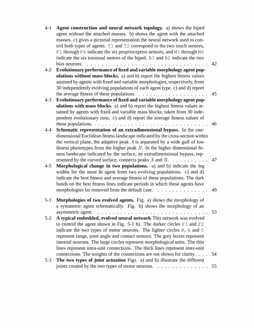
4-1 Agent construction and neural network topology. a) shows the bipedagent without the attached masses. b) shows the agent with the attachedmasses. c) gives a pictorial representation the neural network used to con-trol both types of agents.T1 andT2 correspond to the two touch sensors,P1 throughP6 indicate the six proprioceptive sensors, andM1 throughM6indicate the six torsional motors of the biped.B1 andB2 indicate the twobias neurons. . . .. . . . . . . . . . . . . . . . . . . . . . . . . . . . . . 42

4-2 Evolutionary performance of fixed and variable morphology agent pop-ulations without mass blocks.a) and b) report the highest fitness valuesattained by agents with fixed and variable morphologies, respectively, from30 independently evolving populations of each agent type. c) and d) reportthe average fitness of these populations. . . .. . . . . . . . . . . . . . . . 45

4-3 Evolutionary performance of fixed and variable morphology agent pop-ulations with mass blocks.a) and b) report the highest fitness values at-tained by agents with fixed and variable mass blocks, taken from 30 inde-pendent evolutionary runs. c) and d) report the average fitness values ofthese populations. .. . . . . . . . . . . . . . . . . . . . . . . . . . . . . . 46

4-4 Schematic representation of an extradimensional bypass.In the one-dimensional Euclidean fitness landscape indicated by the cross-section withinthe vertical plane, the adaptive peakA is separated by a wide gulf of lowfitness phenotypes from the higher peakB. In the higher dimensional fit-ness landscape indicated by the surface, an extradimensional bypass, rep-resented by the curved surface, connects peaksA andB. . . . . . . . . . . 47

4-5 Morphological change in two populations. a) and b) indicate the legwidths for the most fit agent from two evolving populations. c) and d)indicate the best fitness and average fitness of these populations. The darkbands on the best fitness lines indicate periods in which those agents havemorphologies far removed from the default case. . .. . . . . . . . . . . . 49

5-1 Morphologies of two evolved agents.Fig. a) shows the morphology ofa symmetric agent schematically. Fig. b) shows the morphology of anasymmetric agent. . . . . . . . . . . . . . . . . . . . . . . . . . . . . . . 53

5-2 A typical embedded, evolved neural networkThis network was evolvedto control the agent shown in Fig. 5-1 b). The darker circlesF1 andF2indicate the two types of motor neurons. The lighter circlesR, A andCrepresent range, joint angle and contact sensors. The grey boxes representinternal neurons. The large circles represent morphological units. The thinlines represent intra-unit connections. The thick lines represent inter-unitconnections. The weights of the connections are not shown for clarity. . . . 54

5-3 The two types of joint actuation Figs. a) and b) illustrate the differentjoints created by the two types of motor neurons. . .. . . . . . . . . . . . 55

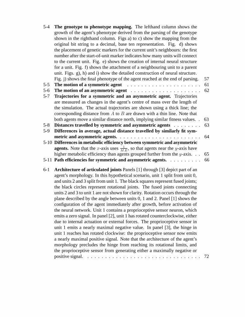
5-4 The genotype to phenotype mapping.The lefthand column shows thegrowth of the agent’s phenotype derived from the parsing of the genotypeshown in the righthand column. Figs a) to c) show the mapping from theoriginal bit string to a decimal, base ten representation. Fig. d) showsthe placement of genetic markers for the current unit’s neighbours: the firstnumber after the start-of-unit marker indicates how many units will connectto the current unit. Fig. e) shows the creation of internal neural structurefor a unit. Fig. f) shows the attachment of a neighbouring unit to a parentunit. Figs. g), h) and i) show the detailed construction of neural structure.Fig. j) shows the final phenotype of the agent reached at the end of parsing. 57

5-5 The motion of a symmetric agent . . . . . . . . . . . . . . . . . . . . . 615-6 The motion of an asymmetric agent . . . . . . . . . . . . . . . . . . . . 625-7 Trajectories for a symmetric and an asymmetric agent. Trajectories

are measured as changes in the agent’s centre of mass over the length ofthe simulation. The actual trajectories are shown using a thick line; thecorresponding distance fromA to B are drawn with a thin line. Note thatboth agents move a similar distance north, implying similar fitness values. . 63

5-8 Distances travelled by symmetric and asymmetric agents. . . . . . . . 635-9 Differences in average, actual distance travelled by similarly fit sym-

metric and asymmetric agents. . . . . . . . . . . . . . . . . . . . . . . . 645-10 Differences in metabolic efficiency between symmetric and asymmetric

agents.Note that thex-axis uses 1M.E

, so that agents near they-axis havehigher metabolic efficiency than agents grouped further from they-axis. . . 65

5-11 Path efficiencies for symmetric and asymmetric agents.. . . . . . . . . 66

6-1 Architecture of articulated joints Panels [1] through [3] depict part of anagent’s morphology. In this hypothetical scenario, unit 1 split from unit 0,and units 2 and 3 split from unit 1. The black squares represent fused joints;the black circles represent rotational joints. The fused joints connectingunits 2 and 3 to unit 1 are not shown for clarity. Rotation occurs through theplane described by the angle between units 0, 1 and 2. Panel [1] shows theconfiguration of the agent immediately after growth, before activation ofthe neural network. Unit 1 contains a proprioceptive sensor neuron, whichemits a zero signal. In panel [2], unit 1 has rotated counterclockwise, eitherdue to internal actuation or external forces. The proprioceptive sensor inunit 1 emits a nearly maximal negative value. In panel [3], the hinge inunit 1 reaches has rotated clockwise: the proprioceptive sensor now emitsa nearly maximal positive signal. Note that the architecture of the agent’smorphology precludes the hinge from reaching its rotational limits, andthe proprioceptive sensor from generating either a maximally negative orpositive signal. . .. . . . . . . . . . . . . . . . . . . . . . . . . . . . . . 72

6-2 Ontogenetic interactions in a developing agentTwo structural units ofan agent are shown above, but only displayed in two dimensions for clarity.For this reason, only four of the six gene product diffusion sites are shown;the other two lie at the top and bottom of the spherical units. The genomeof the agent is displayed, along with parameter values for two genes. Thevalues in parentheses indicate that these values are rounded to integer val-ues. GeneG1 indicates that it is repressed (parameterP1) by concentra-tions of gene product3 (P2) between0.5 and0.99 (P6, P7). Otherwise, itdiffuses gene product22 (P3) from gene product diffusion location4 (P4),indicated in the diagram byC4. Note that genesG1 andG3 emit gene prod-ucts which regulate the other’s expression. The thick dotted lines indicategene product diffusion between diffusion sites within a unit; the thin dottedlines indicate gene product diffusion between units. Both units contain atouch sensor neuron (TS) and a motor neuron (M) connected by excitatorysynapses. . . . . .. . . . . . . . . . . . . . . . . . . . . . . . . . . . . . 74

6-3 Four agent morphologiesThe block is not shown in the figure for the sakeof clarity, but lies just to the left of the agents. The rigid connectors are alsonot shown. The white units indicate the presence of both sensor and motorneurons within that unit. The light gray units indicate the presence of bothsensor and motor neurons in that unit, but the one or more motor neuronsdo not actuate the rotational joint in that unit either because there are noinput connections to the motor neuron, or because there is no joint withinthis unit. The dark gray units indicate the presence of sensor neurons, butno motor neurons. The black units indicate the unit contains neither sensornor motor neurons.. . . . . . . . . . . . . . . . . . . . . . . . . . . . . . 77

6-4 Results from a typical run. Genome length was found to be roughly pro-portional to the number of genes, and is not plotted.. . . . . . . . . . . . 78

6-5 Neural composition of nine evolved agentsEach symbol indicates thenumber of motor and sensor neurons in a structural unit. Neural structureis only reported for units that are part of an appendage. Units comprisingan appendage are linked by gray lines. Gray symbols indicate no rewriterules have been applied to the neural structure in that unit; black symbolsindicate units in which genetic manipulation of local structure has occurred.The gene expression patterns of the four units indicated by bold symbols isshown in Fig. 6-6. Agent1 corresponds to agent b) in Fig. 6-3. .. . . . . 78

6-6 Gene expression patterns for four units.Dark gray and light gray bandscorrespond to periods of gene activity and inactivity, respectively. Fourgenes are marked by asterisks; the expression pattern of these genes is sim-ilar in units a) and c), but different in units b) and d). The expression timesof these genes are darkened for clarity. Genes that are always on or alwaysoff during ontogeny are not shown. Note the evolved gene families, whichhave similar expression patterns.. . . . . . . . . . . . . . . . . . . . . . . 79

7-1 a-e: Images taken fromt0, t75, t150, t225 andt300 during the growth phaseof an evolved agent. The units are darkened in proportion to how manyneurons and synapses they contain.f: t0 of the evaluation phase. The greyunits contain motorized joints. .. . . . . . . . . . . . . . . . . . . . . . . 83

7-2 a: A hypothetical agent at the beginning of growth. The anterior direc-tion (the direction the agent must move in order to gain fitness) is indicated(ANT), as is the posterior direction (POS). A genome, a motor neuron (M)and two maternal TFs (M1, M2) are injected into the single, beginning mor-phological unit (U1). The unit contains six TF diffusion sites (1-6). Thegenome contains five genes:G1, G3, G4 are structural genes;G2 andG5(outlined in bold) are regulatory genes.G3andG5are initially switched on,and begin to diffuse TFs into the unit; the other genes are initially switchedoff (light grey indicates expression; dark grey indicates repression).b: Af-ter several time steps,U1 has split twice, producing neighbouring daugh-ter unitsU2 andU3, which are attached to it by one degree-of-freedomdamped, torsional joints. The genome has been copied intoU2 andU3,where different combinations of TF concentrations have changed the statesof some of the genes.U1 has been lengthened by TF2, which increasesunit length, released byG3 at diffusion site 5.M1 andM2 have diffusedthroughout the unit. The motor neuron inU1 has differentiated into a localneural circuit through combined gene action (T=touch sensor,CPG=centralpattern generator,N=neuron).c: The fully grown agent from which all ge-netic material has been removed, in preparation for agent evaluation. Thejoint nearU2 is active, because it receives motor commands from the neu-ral circuit inU2. The joint nearU3 is passive, and will swing freely duringthe evaluation phase because the motor neuron inU3 has been deleted. . . . 84

7-3 A sample gene.This gene (G3 in Fig. 7-2) emits TF 2 from diffusion site5 (DS5) if it is expressed (the concentration of TF 2 is increased by 0.03at DS5during each time step of the growth phase thatG3 is expressed). Ifthe average concentration of TF 37 in the current unit is between 0.23 and0.93 the gene is expressed; otherwise, it is repressed. The gene is flankedby non-coding values (Nc). . . . . . . . . . . . . . . . . . . . . . . . . . . 86

7-4 The morphology of the most successful agent from one evolutionary run(wild-type). . . . . . . . . . . . . . . . . . . . . . . . . . . . . . . . . . . 88

7-5 The underlying GRN specifying the growth of the agent shown in Figure 7-4. 89

7-6 Results from a lesion experiment. a, The agent regrown with regulatorygenes 10, 34, 35, 60 and 63 repressed in all units (loss-of-function).b,The agent regrown with the targetted genes expressed in all units (gain-of-function). c, Differences in gene expression between the first units ofthe wild-type and loss-of-function agents. Black bars indicate the target-ted regulatory genes; dark grey bars indicate structural genes that influenceneural growth; grey bars indicate structural genes that influence morpho-logical growth; light grey bars indicate other regulatory genes.d, Dif-ferences in gene expression between the first units of the wild-type andgain-of-function agents. . . . . .. . . . . . . . . . . . . . . . . . . . . . . 90

7-7 Plot of neurological versus morphological effect from 60 lesion experi-ments.The filled triangle, square and circle correspond to the agents shownin Figs. 7-1f, 7-4 and (inset). The open triangle, square and circle corre-spond to the first agents appearing in these three evolutionary runs thatcontained the targetted regulatory gene.(inset): The evolved agent withthe most actuated joints. . . . .. . . . . . . . . . . . . . . . . . . . . . . 92

8-1 a-e: Images taken fromt0, t75, t150, t225 andt300 during the growth phaseof an evolved agent. The units are darkened in proportion to how manyneurons and synapses they contain.f: t0 of the evaluation phase. The greyunits contain motorized joints; the dark grey units are in contact with theground plane. . . .. . . . . . . . . . . . . . . . . . . . . . . . . . . . . . 96

8-2 a: A hypothetical agent at the beginning of growth. The anterior direc-tion (the direction the agent must move in order to gain fitness) is indicated(ANT), as is the posterior direction (POS). A genome, a motor neuron (M)and two maternal TFs (M1, M2) are injected into the single, beginning mor-phological unit (U1). The unit contains six TF diffusion sites (1-6). Thegenome contains five genes:G1, G3, G4 are structural genes;G2 andG5(outlined in bold) are regulatory genes.G3andG5are initially switched on,and begin to diffuse TFs into the unit; the other genes are initially switchedoff (light grey indicates expression; dark grey indicates repression).b: Af-ter several time steps,U1 has split twice, producing neighbouring daugh-ter unitsU2 andU3, which are attached to it by one degree-of-freedomdamped, torsional joints. The genome has been copied intoU2 andU3,where different combinations of TF concentrations have changed the statesof some of the genes.U1 has been lengthened by TF2, which increasesunit length, released byG3 at diffusion site 5.M1 andM2 have diffusedthroughout the unit. The motor neuron inU1 has differentiated into a localneural circuit through combined gene action (T=touch sensor,CPG=centralpattern generator,N=neuron).c: The fully grown agent from which all ge-netic material has been removed, in preparation for agent evaluation. Thejoint nearU2 is active, because it receives motor commands from the neu-ral circuit inU2. The joint nearU3 is passive, and will swing freely duringthe evaluation phase because the motor neuron inU3 has been deleted. . . . 97

8-3 A sample gene.This gene (G3 in Fig. 8-2) emits TF 2 from diffusion site5 (DS5) if it is expressed (the concentration of TF 2 is increased by 0.03at DS5during each time step of the growth phase thatG3 is expressed). Ifthe average concentration of TF 37 in the current unit is between 0.23 and0.93 the gene is expressed; otherwise, it is repressed. The gene is flankedby non-coding values (Nc). . . . . . . . . . . . . . . . . . . . . . . . . . . 98

8-4 Phenotype and genotype of the most fit agent. a: The morphology ofthe most fit agent evolved from among 60 independent evolutionary runs.Light gray units contain active motors; dark gray units are in contact withthe ground plane.b: The genetic regulatory network from which this agentwas grown. Boxes indicate genes; directed edges indicate gene regulation. 102

8-5 Evolutionary change of gene networks. a: The phylogenetic history ofthe run which produced this agent. The line with box markers indicatesthe best fitness curve for this run. The thick line denotes the proportion ofgenes which lie along a cyclical gene pathway in the GRN taken from thefittest agent for that generation. The thin line denotes the average number ofgenes lying along cyclical gene pathways for random GRNs with the samenumber of genes and gene interactions as the GRN taken from the fittestagent for that generation. The vertical line indicates the generation in whichthe first agent receives fitness based on its behaviour.b: Magnification ofa. 103

8-6 GRN properties for agents from different runs. The fittest agent wastaken from each of the 60 evolutionary runs, and the cyclicality of theirGRNs, as compared with random graphs with the same number of nodesand edges, is plotted against that agent’s fitness. . . .. . . . . . . . . . . . 103

8-7 Direct evolution of cyclicality. a: The thick line indicates the cyclicality ofthe fittest GRN in the population at each generation. The thin line denotesthe number of floating-point values contained in the fittest genome.b: Thegenetic regulatory network constructed from the fittest genome in the firstgeneration. Thick-lined circles indicate regulatory genes; thin-lined circlesindicate structural genes. Directed edges indicate gene regulation.c: Thegenetic regulatory network constructed from the fittest genome taken fromthe final generation.. . . . . . . . . . . . . . . . . . . . . . . . . . . . . . 104

9-1 Morphogenesis and neurogenesis.This figure shows a hypothetical growthprogramme for a simple robot. The upper panel shows the state of therobot at the beginning of growth: two morphological units are attached toeach other, all genes are turned off, and two different chemicals that regu-late gene expression (TF25 and TF26) are injected into the units to initiategrowth. In the lower panel, several time steps have elapsed, and some mor-phogenesis and neurogenesis has occurred. The states of the genes havediverged in different units (black bars indicate expressed genes; gray barsindicate non-expressed genes; white tracts indicate non-coding regions).Several neurons (gray filled circles) have been created (T = touch sensorneurons,A = angle sensor neurons,M = motor neurons, unmarked = in-ternal neurons). Synapses (arrows) have grown and split, and some haveattached to target neurons. A rotational joint has grown between two units(U2 andU4); the motorized joint is receiving commands from a motor neu-ron (M in U2), and feeding its current angle into the angle sensor neuron(A in U2). A neural circuit spanning three units has grown, starting fromthe touch sensor inU1, feeding into the motorized joint inU2, and contin-uing via the angle sensor neuron inU1 into the motor neuron inU4. AsU4does not contain a motorized joint, this part of the circuit does not affectbehaviour, and is thus neutral, along with the unattached synapses inU2(the active synapses of the circuit are drawn in bold).. . . . . . . . . . . . 111

9-2 Pseudocode for the genetic algorithm.The algorithms for growing andevaluating a robot are shown in Figure 9-5. .. . . . . . . . . . . . . . . . 112

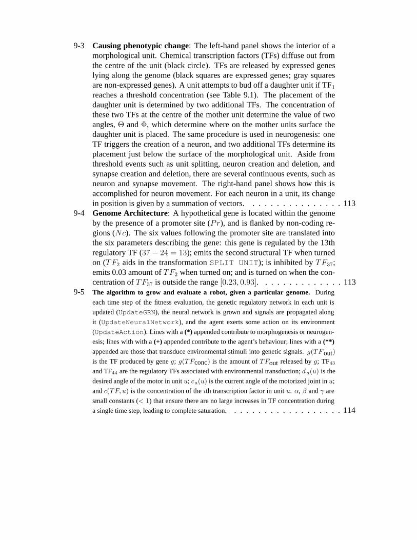
9-3 Causing phenotypic change: The left-hand panel shows the interior of amorphological unit. Chemical transcription factors (TFs) diffuse out fromthe centre of the unit (black circle). TFs are released by expressed geneslying along the genome (black squares are expressed genes; gray squaresare non-expressed genes). A unit attempts to bud off a daughter unit if TF1

reaches a threshold concentration (see Table 9.1). The placement of thedaughter unit is determined by two additional TFs. The concentration ofthese two TFs at the centre of the mother unit determine the value of twoangles,Θ andΦ, which determine where on the mother units surface thedaughter unit is placed. The same procedure is used in neurogenesis: oneTF triggers the creation of a neuron, and two additional TFs determine itsplacement just below the surface of the morphological unit. Aside fromthreshold events such as unit splitting, neuron creation and deletion, andsynapse creation and deletion, there are several continuous events, such asneuron and synapse movement. The right-hand panel shows how this isaccomplished for neuron movement. For each neuron in a unit, its changein position is given by a summation of vectors. . . .. . . . . . . . . . . . 113

9-4 Genome Architecture: A hypothetical gene is located within the genomeby the presence of a promoter site (Pr), and is flanked by non-coding re-gions (Nc). The six values following the promoter site are translated intothe six parameters describing the gene: this gene is regulated by the 13thregulatory TF (37− 24 = 13); emits the second structural TF when turnedon (TF2 aids in the transformationSPLIT UNIT); is inhibited byTF37;emits 0.03 amount ofTF2 when turned on; and is turned on when the con-centration ofTF37 is outside the range[0.23, 0.93]. . . . . . . . . . . . . . 113

9-5 The algorithm to grow and evaluate a robot, given a particular genome. During

each time step of the fitness evaluation, the genetic regulatory network in each unit is

updated (UpdateGRN), the neural network is grown and signals are propagated along

it (UpdateNeuralNetwork), and the agent exerts some action on its environment

(UpdateAction). Lines with a(*) appended contribute to morphogenesis or neurogen-

esis; lines with with a(+) appended contribute to the agent’s behaviour; lines with a(**)

appended are those that transduce environmental stimuli into genetic signals.g(TFout)is the TF produced by geneg; g(TFconc) is the amount ofTFout released byg; TF43

and TF44 are the regulatory TFs associated with environmental transduction;da(u) is the

desired angle of the motor in unitu; ca(u) is the current angle of the motorized joint inu;

andc(TF, u) is the concentration of theith transcription factor in unitu. α, β andγ are

small constants (< 1) that ensure there are no large increases in TF concentration during

a single time step, leading to complete saturation.. . . . . . . . . . . . . . . . . . 114

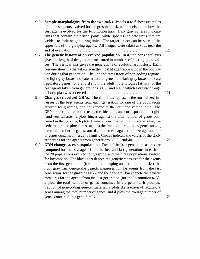
9-6 Sample morphologies from the two tasks.Panelsa to f show examplesof the best agents evolved for the grasping task, and panelsg to i show thebest agents evolved for the locomotion task. Dark gray spheres indicateunits that contain motorized joints; white spheres indicate units that arewelded to their neighbouring units. The target object can be seen to theupper left of the grasping agents. All images were taken att400, near theend of evaluation. . . . . . . . . . . . . . . . . . . . . . . . . . . . . . . 120

9-7 The genetic history of an evolved population.In a, the horizontal axisgives the length of the genome, measured in numbers of floating-point val-ues. The vertical axis gives the generations of evolutionary history. Eachgenome shown is that taken from the most fit agent appearing in the popula-tion during that generation. The line indicates tracts of non-coding regions;the light gray boxes indicate structural genes; the dark gray boxes indicateregulatory genes.b, c andd show the adult morphologies (at t400) of thebest agents taken from generations 30, 35 and 40, in which a drastic changein body plan was observed. . .. . . . . . . . . . . . . . . . . . . . . . . 121

9-8 Changes to evolved GRNs: The thin lines represent the normalized fit-nesses of the best agents from each generation for one of the populationsevolved for grasping, and correspond to the left-hand vertical axis. TheGRN properties are plotted using the thick line, and correspond to the right-hand vertical axis.a plots fitness against the total number of genes con-tained in the genome,b plots fitness against the fraction of non-coding ge-netic material,c plots fitness against the fraction of regulatory genes amongthe total number of genes, andd plots fitness against the average numberof genes contained in a gene family. Circles indicate the values of the GRNproperties for the agents from generations 30, 35 and 40. . . . . .. . . . . 122

9-9 GRN changes across populations: Each of the four genetic measures arecomputed for the best agent from the first and last generations in each ofthe 20 populations evolved for grasping, and the three populations evolvedfor locomotion. The black bars denote the genetic measures for the agentsfrom the first generation (for both the grasping and locomotion tasks), thelight gray bars denote the genetic measures for the agents from the lastgeneration (for the grasping task), and the dark gray bars denote the geneticmeasures for the agents from the last generation (for the locomotion task).a plots the total number of genes contained in the genome,b plots thefraction of non-coding genetic material,c plots the fraction of regulatorygenes among the total number of genes, andd plots the average number ofgenes contained in a gene family. . . . . . .. . . . . . . . . . . . . . . . 123

9-10 Effect of suppressing environmental transduction during growth.Theupper row shows the growth of the most fit agent from one of the evolvedpopulations for grasping. Still frames are taken at time steps 10 (t10), t20,t50, t100, t200 andt400. The lower row shows the effect of re-growing thisagent, but suppressing environmental stimuli from being transduced intothe two corresponding chemicals TF43 and TF44. . . . . . . . . . . . . . . 124

9-11 Lesion effects on evolved agents.Panela corresponds to the populationwhich evolved the agent shown in Figure 9-10. Panelb corresponds to thepopulation which evolved the agent shown in Figure 9-6c. Each columncorresponds to the lesion effects on the most fit agent present in the popu-lation at that generation. A filled square indicates that that particular lesionhad an effect on fitness, and thus contributed to the growth of that agent.Blank areas indicate that that particular lesion did not affect the fitness ofthat agent, and thus did not contribute to the growth of that agent. Each rowcorresponds to a particular lesion experiment. The lowest row correspondsto suppressing genes that produce TF24 during growth, the second row cor-responds to suppressing genes that produce TF25 during growth, and so on.The row marked with a filled diamond corresponds to suppressing genesthat produce TF43 during growth. The row marked with a filled trianglecorresponds to suppressing the transduction of joint stress into TF43. Therow marked with a filled circle corresponds to suppressing genes that pro-duce TF44 during growth. The row marked with a filled square correspondsto suppressing the transduction of touch information into TF44. . . . . . . 125

9-12 Generalized lesion effects across all evolved populations.The 22 lesionexperiments were performed on the best agent from each generation, forall 20 populations evolved for grasping. The probability that a particularlesion would have an effect on fitness was calculated for each lesion, foreach generation. The darker regions indicate greater probability, such thatblack squares correspond to particular lesions that had a fitness effect onall of the best agents extracted from the 20 populations, for that generation.The lowest row corresponds to suppressing genes that produce TF24 dur-ing growth, the second row corresponds to suppressing genes that produceTF25 during growth, and so on. The row marked with a filled diamond cor-responds to suppressing genes that produce TF43 during growth. The rowmarked with a filled triangle corresponds to suppressing the transductionof joint stress into TF43. The row marked with a filled circle correspondsto suppressing genes that produce TF44 during growth. The row markedwith a filled square corresponds to suppressing the transduction of touchinformation into TF44. . . . . . . . . . . . . . . . . . . . . . . . . . . . . 126

9-13 Onset of evolutionary appropriation of environmental stimuli. Panelaoutlines the role of TF43 in guiding growth for the 20 populations evolvedfor grasping. The diamonds indicate the first generation in which the growthof the most fit agent in the population at that time was influenced by geneticproduction of TF43. The triangles indicate the first generation in whichthe growth of the most fit agent in the population was influenced by envi-ronmental production of TF43. The thick lines indicate the length of evo-lutionary time until the other source of TF43 was also exploited to guidegrowth. Thick lines that do not terminate with a symbol indicate that theother source was never exploited. Panelb outlines the role of TF44 in guid-ing growth. The circles indicate the first generation in which the growth ofthe most fit agent in the population was influenced by genetic productionof TF44. The squares indicate the first generation in which the growth ofthe most fit agent in the population was influenced by environmental pro-duction of TF44. The thick lines indicate the length of evolutionary timeuntil the other source of TF44 was also exploited to guide growth. Thicklines that do not terminate with a symbol indicate that the other source wasnever exploited. The thin lines indicate those populations for which neitherof the sources of TF44 were made use of to guide growth. . . . . .. . . . . 127

9-14 The internal neural circuits of a sample agent. aprovides a magnifica-tion of the centre of the agent shown in its entirety in Figure 9-6b. b showsthe internal neural structure of this part of the agent. Large black circles in-dicate the centres of morphological units; black lines indicate connectedneighbouring units; smaller circles indicate neurons; dark gray lines indi-cate synapses that connect to neurons; light gray lines indicate unconnectedsynapses. . . . . .. . . . . . . . . . . . . . . . . . . . . . . . . . . . . . 128

10-1 Three different encoding schemes for evolving robots.A parametricencoding scheme is shown ina, in which one part of the genome corre-sponds to only one phenotypic structure. A recursive encoding scheme isshown inb, in which one part of the genome can correspond to one ormore (possibly higher-order) phenotypic structures. A developmental en-coding scheme is shown inc, in which genomes, encoded as GRNs, initiatedynamic processes which over the growth period of the agent can lead to re-peated (possibly higher-order) phenotypic structures. In this scheme, eachunit contains a copy of the genome, but gene states may vary across units:expressed genes are drawn in black, and non-expressed genes in gray. . . . 148

10-2 Generation of locomotion with repeated reactive neural structure. ashows the internal neural structure of an appendage, with the distal tip tothe left, and the proximal root (where it attaches to the robot’s main body)to the right. Sensor neurons are indicated byS; motor neurons are indi-cated byM; activated neurons are drawn dark gray; inactivated neurons aredrawn light gray; and activated synapses are drawn in bold.b shows howthe combination of this circuitry leads to forward motion: the backwardstraveling wave generates forward motion. . .. . . . . . . . . . . . . . . . 150

10-3 Three possible genetic regulatory network architectures. ashows anacyclical architecture in which separate regulatory genes (bold boxes) inde-pendently regulate structural genes (thin boxes).b shows another acyclicalarchitecture, which is hierarchical: a few regulatory genes regulate sub-groups of regulatory and structural genes.c shows a cyclical architecture,in which no regulatory gene has a higher influence over growth than an-other. . . . . . . . . . . . . . . . . . . . . . . . . . . . . . . . . . . . . . 153

10-4 The internal neural circuits of a sample agent. aprovides a magnifica-tion of the centre of the agent shown in its entirety in Figure 9-6b. b showsthe internal neural structure of this part of the agent. Large black circles in-dicate the centres of morphological units; black lines indicate connectedneighbouring units; smaller circles indicate neurons; dark gray lines indi-cate synapses that connect to neurons; light gray lines indicate unconnectedsynapses. . . . . .. . . . . . . . . . . . . . . . . . . . . . . . . . . . . . 154

List of Tables

4.1 The default size dimensions, masses and joint limits of the biped.Pa-rameters set in boldface indicate those parameters that are modified by evo-lution in the experiments reported in section 4.3. The valid ranges for theseparameters are also given. . . . .. . . . . . . . . . . . . . . . . . . . . . . 43

4.2 Experimental regime summary. . . . . . . . . . . . . . . . . . . . . . . 45

9.1 phenotypic transformations triggered by the structural TFS. ( D = Discrete,C = Continuous ) .. . . . . . . . . . . . . . . . . . . . . . . . . . . . . . 110

xix

Chapter 1

Introduction

This thesis is a direct result of two recent intellectual revolutions (evolutionary robotics andembodied Artificial Intelligence) and one new computer technology (physical simulation).

Briefly, evolutionary robotics is an attempt to use evolutionary computation to automatethe design of intelligent robots. However, because evolutionary computation requires theevaluation of many potential solutions for any given problem, this poses two major chal-lenges for the field. First, the sheer amount of time required to iteratively test potentialcontrollers on one robot is prohibitive. Second, the problem becomes near impossible ifthe designer wishes to try out different robot body plans, as well as different controllers,because the robots must then be built from scratch, and the construction of a single robotcan often take weeks, or months.

The nascent field of embodied Artificial Intelligence (embodied AI) is a response toclassical Artificial Intelligence, which held that intelligence could be generated by suffi-ciently complex and purely computational algorithms. Embodied AI is the realization thatintelligent behaviour is the result of an agent’s interaction with its environment, and thatthis interaction is mediated by both the agent’s body and its brain. It follows from thisthat a robot designer can not simply choose a robot body haphazardly and tinker with itscontroller in order to generate intelligent behaviour. Rather, decisions about the robot’smorphology must also be taken into account during the design process. However the samechallenge arises here as in evolutionary robotics: it is difficult to continuously build differ-ent robots and combine them with candidate controllers in the hopes of producing intelli-gent behaviour.

Here we document a series of experiments in which evolutionary computation is usedto generate large numbers of morphologies and neural controllers for simulated robots thatact in a virtual, yet physically realistic environment. By simulating the robots, it is possibleto drastically speed up the time required to ’construct’ a robot, and test it in a physicalenvironment. By allowing artificial evolution to tune the relationships between a robot’sbody, its brain, and its interaction with its environment, we are able to uncover severalinterdependencies between brain and body in particular, and how these two subsystemswork together to generate intelligent behaviour in general.

1

Figure 1-1:Algorithmic flow of a basic genetic algorithm.

1.1 Evolutionary Computation

Evolutionary computation [Back et al., 1997, Foster, 2001] began as a biologically-inspiredtechnique for numerical optimization [Bremermann, 1962], as well as for optimization ofengineered systems. Three main techniques appeared roughly contemporaneously: evolu-tionary programming [Fogel et al., 1966], genetic algorithms [Holland, 1975], and evolu-tion strategies [Rechenberg, 1994]. Since that time, evolutionary computation has maturedinto a field of study in its own right [Goldberg, 1989, Koza, 1992].

It is important to note that evolutionary computation is, in most cases, an engineeringtool, rather than an attempt to model evolutionary dynamics. This distinction will ariseoften in this thesis: all of the experiments reported here are attempts to model aspects ofbiology in order to automate the design of robots, not to model aspects of biology in orderto prove or refute biological hypotheses. In its simplest and most general form, all threebranches of evolutionary computation act as follows: they rely on populations of solutionsfor a given problem; fitness is a quantitative measure used to judge the relative performanceof one solution over another; and selection relies on deletion of poor solutions, and modifiedcopying of better solutions. Starting with a random population of solutions and iterativelyapplying fitness evaluation followed by selection, eventually increasingly better solutionsappear in the population, and the algorithm terminates when some user-defined criterion ismet, such as a fixed number of solution evaluations, or a desired level of solution quality.

In this thesis all of the experiments are based on the genetic algorithm (GA) [Holland, 1975,Goldberg, 1989]. The basic algorithmic flow of a generational GA is given in Figure 1-1.The primary characteristic of GAs is that the genotype (the genetic information) is encoded

in a linear string of symbols, or numbers: what these values represent is defined by the GAdesigner, and is known as the encoding of the GA. The translation of the genotype into thesolution to be evaluated, or the phenotype, is known as the genotype-to-phenotype map-ping. The encoding, the genotype-to-phenotype mapping, and the formula chosen to trans-late a solution’s performance into a number (known as the fitness function), vary greatlyfrom one instantiation of a GA to another, and these three issues lie at the core of geneticalgorithm, and indeed evolutionary computation research. In the experiments describedhere, various encodings, mappings and fitness functions are employed, and are describedin detail for each experiment.

In contrast to these three aspects of GAs, however, the methods of selection and re-production are very similar across all of the experiments described. Several methods ofselection exist, but most rely on a statistically biased sampling of more fit genotypes1 overless fit genotypes. Once a genome has been selected, a copy of it is made and two typesof reproduction can be applied: mutation and recombination. Mutation entails the replace-ment or modification of one or more of the values stored in the genome. Larger mutationoperators, such as genome rearrangement, are also possible, and are used in the work pre-sented here. Recombination entails the combination of parts of both parents into the newgenomes.

Figure 1-2 documents this process for both fixed-length GAs, in which the numberof values encoded in the genome remains fixed during evolution, and for variable-lengthGAs, in which either the user [Harvey, 1992] or selection pressure (through the processof unequal crossover) is capable of modifying the length of the genome. In the case ofunequal crossover, other pressures besides selection pressure can modify genome lengthover evolutionary time, such as genetic drift. This process is known in the evolutionarycomputation literature as bloat [Lones and Tyrrell, 2002], which often leads to the gradualincrease in genome size over evolutionary time.

In order to study the interdependencies between robot body and brain for the generationof intelligent behaviour, various types of GA encodings, genotype-to-phenotype mappings,fitness functions, selection schemes and mutational and recombination operators are em-ployed in this thesis. In later chapters, a model of ontogeny—artificial ontogeny—is incor-porated into the genetic algorithm, which requires a radical departure from the more wellknown types of genotype to phenotype mappings. It is the implementation and subsequentstudy of this mapping that forms the crux of this thesis.

1.2 Evolutionary Robotics

Evolutionary robotics is the attempt to employ evolutionary computation for the automateddesign of intelligent robots [Harvey et al., 1997, Nolfi and Floreano, 2000]. Usually, an

1We concede that genotypic fitness is a confusing term, as it is the action of the phenotype in its envi-ronment that generates fitness. Genotypic fitness is here used as shorthand for the fitness of a phenotypegenerated by a particular genotype.

Figure 1-2: Recombination in genetic algorithms. The upper panel shows equalcrossover, which produces two child genomes (C1 and C2) that are equal in length tothe two parent genomes (P1 andP2). The crossover point is indicated by the two arrows.In the lower panel, unequal crossover can lead to child genomes with lengths differing fromtheir parent genomes, and each other.

evolutionary robotics experiment proceeds as follows. A particular robot is chosen (of-ten the hockey-puck sized two-wheeled Khepera2), along with a desired behaviour. A fit-ness function is formulated that quantifies the robot’s behaviour. Then, some aspect of therobot’s controller is translated into a set of parameters, which are collected into a genotype,and supplied to a genetic algorithm.

For each genome in the population, the values are used to modify the robot’s con-troller, and the robot is then allowed to act in its environment. The resulting behaviouris evaluated using the fitness function, and the fitness value of the responsible genomeis assigned. As successive evaluations proceed, selection and reproduction are appliedto the genomes in the population. Figure 1-3 outlines the basic procedure of an evo-lutionary robotics experiment. In a successful experiment, the robot’s behaviour beginsto improve over time as the genetic algorithm converges on a fit collection of controllerparameters. The evaluations of the candidate controllers can be done on a real robot[Cliff et al., 1993, Floreano and Mondada, 1998], or as is more often the case, a computersimulation of the robot and its environment are used. Simulation is often employed because

2Developed and distributed by K-Team SA, Switzerland

Figure 1-3:Algorithmic flow of an evolutionary robotics experiment.

of the prohibitive time costs for iteratively evaluating candidate controllers on a real robot,as well as the awkwardness of resetting the robot after each evaluation. Chapters 2 and3 present relatively standard evolutionary robotics experiments: the synaptic weights ofneural controllers for robots with fixed body plans are treated as parameters to be evolvedusing a genetic algorithm.

As noted earlier, the tendency to only evolve brains, as opposed to bodies of robots isdue to the practical difficulties in testing large numbers of different robots. However, ithas been pointed out that there are other reasons for this. First, most of the tasks requiredof evolved robots are simple enough to be solved with a functionally-limited morphology[Lipson, 2001]. For example, most tasks tackled so far in evolutionary robotics requirelocomotion over flat, smooth terrain: it is obvious that this can be accomplished with awheeled robot, such as the Khepera. However, as tasks become more challenging, it be-comes more difficult to predict what morphology is required for the given task. A secondreason for this bias is due to the close relation between evolutionary robotics and ArtificialIntelligence (AI).

1.3 Embodied Artificial Intelligence

Since its founding [Turing, 1950], one of the underlying, implicit assumptions of Artifi-cial Intelligence was that symbol processing in the brain is the sole generator of intelligentbehaviour. Several reasons have been cited for this bias, including an over-reliance onthe metaphor of the brain as an information processing computer borrowed from cognitivescience [Pfeifer and Scheier, 1999], and the legacy of Cartesian dualism, which holds thatthe brain and the body are independent, separable sub-systems. However, in recent years

it has been noted [Brooks, 1990, Brooks, 1991c, Brooks, 1991b, Hendriks-Jansen, 1996,Pfeifer and Scheier, 1999] that an agent’s morphology—its body shape, material proper-ties, and sensory and motor complement—is an integral aspect of intelligent behaviour.This realization has led to the emergence of a revolution in Artificial Intelligence: Embod-ied AI.

The main tenet of Embodied AI is that an intelligent agent (whether it be a biologicalorganism or robot) must be bothembodiedandsituated3. An embodied agent possesses aphysical body that allows it to act on, and be acted upon by, its surroundings in some ways,but not others. For example, a heavy, legged robot must concern itself with maintainingbalance, but may traverse both flat and rugged terrain. A wheeled robot, in contrast, neednot worry about self balance, but it is limited to traversing flat terrain.

A situated agent is equipped with a set of sensors that allow it to extract informationfrom its environment. Situated agents must make sense of the flood of real-time, raw dataarriving on its sensors, whereas non-situated agents are often provided with higher-levelsemantic information by the agent’s designer.

Because robot bodies and sensors are physical objects, it has been argued that progressin embodied AI can only be achieved by working with physical robots acting in the realworld, as opposed to simulated robots acting in virtual worlds [Brooks, 1990]. Again, how-ever, this requires the painstaking trial and error methodology of building and continuallymodifying physical robots.

1.4 Combining Them: Physical Simulation

With the recent advent of computer software known as physical simulation, it has becomepossible to simulate, instead of actually build, embodied and situated robots. In this thesis,two physical simulator packages are used (the commercial package MathEngine4, and theopen-source package Open Dynamics Engine (ODE)5). At root, these packages work simi-larly. A three-dimensional world is simulated, to which the user can add or remove objects.During each time step, the forces acting upon an object in this world are computed, such asgravity, inertia, momentum and friction, and the object’s position, velocity and orientationare updated based on these forces. If objects come into contact with one another, collisiondetection and resolution algorithms keep the objects from interpenetrating. Further, objectscan be attached to one another with a variety of joint types, such as rotational joints (likethe human elbow or knee joints) and ball-and-socket joints (like the human shoulder joint).Finally, virtual motors can be attached to the joints, which apply torque to the connectedobjects, and further influence their relative motion. By writing additional program code tosimulate various types of sensors, an embodied, situated robot can be tested in a ’physical’

3There are other aspects of an agent, such as autonomy, that are also cited as important, but these aspectsare not treated directly in this thesis. For example, it is a matter of debate whether a virtual robot is, or canever be autonomous.

4CMLabs Simulations, Inc.5www.q12.org

Figure 1-4: Translating simulated robot behaviours to a real robot. In [Frutiger etal., 2002] we demonstrated that it was possible to translate an evolved behaviour for asimulated brachiating robot to a real robot. Both the simulated and real robot contain afreely swinging joint (the joint connecting the lower ‘leg’ to the torso) which is exploitedfor producing forward momentum, and thus the locomoting behaviour.

environment. In the following chapters, a more detailed description of how evolutionaryrobotics experiments can be carried out in a physical simulator is given.

The main argument underlying embodied AI is that progress in the field can onlybe made by testing hypotheses on real robots acting in the real world [Brooks, 1991a,Pfeifer and Scheier, 1999]. It is argued that simulation introduces abstractions about therobot and its environment, and often behaviours observed in simulation do not translate onto real robots, because these robots encounter environmental effects that were not experi-enced during simulation. For example, a virtual robot may locomote well over a perfectlysmooth and flat ground plane in simulation, but the locomotion strategy may fail on a realrobot that must traverse over ground surfaces that are never perfectly smooth nor flat. Thechallenge of this transferral from simulation to the real world is often referred to as ‘cross-ing the reality gap’, and several strategies for achieving this transferral have been proposed[Jakobi, 1997, Floreano and Mondada, 1998]. This thesis does not deal with this issue di-rectly, but assumes that it may be possible to augment the simulation experiments presentedhere in order to transfer the evolved body plans and neural controllers to the real robot, andhave it successfully reproduce the observed behaviour.

Initial experiments have shown that this is indeed possible: in [Frutiger et al., 2002]we have demonstrated that it is possible to translate an evolved behaviour for a simulatedbrachiating robot (a robot that swings from one overhead hold to another using its arms) toa real robot. Figure 1-4 shows the evolved behaviour for the simulated robot, as well as thebehaviour of the real robot when the evolved control strategy is transferred to it. Moreover,both the simulated and real robot make use of passive dynamics [McGeer, 1990], which isthe exploitation of freely swinging joints for generating locomotion. However as this thesisdoes not deal explicitely with the issue of transferral from simulation to reality, the detailsof this experiment are not discussed here.

1.5 Evolving Brain and Body

As simulation technology advances, it has become faster and simpler to evolve and eval-uate the behaviour of virtual robots with differing morphologies as well as controllers.One of the first examples of this was the evolution of sensory morphologies for a visuallyguided robot in a simple simulation [Cliff et al., 1993]. Another early experiment in thefield that gained wide recognition [Sims, 1994] placed more aspects of the morphology—including the body plan, and sensor and motor placements—under evolutionary control.Sims programmed his own physical simulator for which to evaluate the evolved virtualrobots: unfortunately, details regarding the simulator itself are not available. The simulatorwas run on a Connection Machine parallel computer [Hillis, 1985], which contained 65,536processors. Sims was able to evolve agents to walk, swim, jump, and compete against asingle opponent for possession of a common resource. Figure 1-5 shows three hypotheticalagents, and the structure of the genomes that could produce them. Note that the genomesare not simply strings of numbers, but are recursive structures: that is, the same part of thegenome can specify more than one part of the phenotype. This lends two desirable prop-erties to the artificial evolutionary process: first, the amount of information in the genomedoes not necessarily have to scale with the amount of phenotypic structure, and there is anexplicit bias that favours repeated phenotypic structures. These two issues—genetic com-pression and repeated phenotypic structure—will serve as the main foci in the final fourchapters of this thesis.

Two other recursive genetic encoding schemes have been proposed since Sims’ work,with satisfactory results: both projects have spawned complex agents with repeated pheno-typic structures (for an example see Figure 1-5), and the agents exhibit some interesting,non-trivial behaviours such as locomotion, and following moving objects [Adamatzky etal., 2000, Hornby and Pollack, 2002].

Others have employed development in order to ‘grow’ robot brains and bodies together[Delleart and Beer, 1994, Jakobi, 1995, Bentley and Kumar, 1999]. These approaches aresimilar in that the genotype to phenotype translation begins with a simple phenotype madeup of one or more modules. These modules can be parts of the robot’s body or brain. Thegenotype then initiates a series of transformations that are carried out in parallel on all ofthe modules comprising the phenotype. This leads to a proliferation and differentiation ofthe modules. This abstraction of development (the parallel genetic transformation of phe-notypic modules) stems from the early work of Aristid Lindenmayer [Lindenmayer, 1968],who devised the mathematical formulation known as L-systems [Prusinkiewicz and Linden-mayer, 1990] for modeling plant morphogenesis.

In the developmental schemes mentioned above, it is not clear what the phenotypicmodules represent. Furthermore, it is assumed that parallel, recursive application of rewriterules is a useful model of biological development that will facilitate the artificial evolutionof robots. Eggenberger first introduced a much more biologically realistic developmen-tal model for growing three-dimensional structures [Eggenberger, 1997]. In this work, thephenotypic modules closely resemble biological cells: each cell contains a complete copy

Figure 1-5:The genotype to phenotype translation in Sims’ work (from [Sims, 1994]).

of the genome; the genes contained in the genome diffuse gene products through the cell,and into neighbouring cells (possibly leading to cell communication); the same gene maybe expressed in some cells, but not in others (possibly leading to cell differentiation). Inthe last four chapters of this thesis, Eggenberger’s basic model is extended to include neu-rogenesis. Thus, both robot brains and bodies can be evolved together, and it is possibleto exert selection pressure on the robot’s behaviour, not just on its morphology. For theremainder of this thesis, we refer to this more biologically plausible model of developmentasartificial ontogeny6.

The relative merits of these two models of development will be taken up later in thisthesis, but the main aim is to lend support to the second model. We will show that: thetwo advantages of recursive genetic encoding schemes—genetic compression and repeated

6I regard artificial ontogeny (AO) as more biologically plausible that recursive developmental modelsbecause AO relies on more detailed biological mechanisms for achieving growth, such as differential geneexpression, transcription factor diffusion throughout the body, and the ability for the agent to grow and adaptduring its lifetime.

phenotypic structure—naturally emerge in artificial ontogeny; and that artificial ontogenyhas an additional advantage, which is the ability to modify morphogenesis and/or neuroge-nesis in response to environmental stimuli.

1.6 Contributions

Physical simulation technology allows for a dramatic decrease in the total time required to’construct’ robots and evaluate their behaviour. This in turn allows for advances to be madein both evolutionary robotics and embodied AI. Indeed this thesis documents several suchadvances, which are derived from a series of evolutionary robotics experiments:

• how artificial evolution can sequentially integrate different sensor modalities for thegeneration of behaviour (Chapter 2);

• a methodology for systematically uncovering the behavioural constraints and oppor-tunities implied by a chosen robot body plan (Chapter 3);

• how the inclusion of morphological parameters into the genome can facilitate theevolutionary process, despite the increased dimensionality of the search space (Chap-ter 4);

• clarification of one particular interdependence between morphology (body symme-try) and behaviour (directed locomotion) (Chapter 5);

• further support for the claim that a well chosen robot morphology can reduce theamount of neural control required [Lichtensteiger and Eggenberger, 1999] (Chapter6);

• how artificial ontogeny facilitates the evolution of a robot’s body and brain together(Chapters 6, 7, 8 and 9).

• artificially evolved GRNs tend to exhibit hierarchical architectures (Chapter 8);

• artificial ontogeny is scalable, insofar as it dissociates genotypic complexity fromphenotypic complexity (Chapters 6 and 9);

• artificial ontogeny makes use of the neutrality inherent to the system (Chapter 9);

• and how environmental stimuli is be made available to, and appropriated by artificialevolution in order to guide growth (Chapter 9).

1.7 Overview of the Thesis

This thesis is organized around eight published papers, which form chapters 2 to 8. Thefirst experiment, described in chapter 2, documents a standard evolutionary robotics exper-iment, closely following the experimental flow shown in Figure 1-3. Succeeding chaptersintroduce experiments in which more aspects of the robot’s controller, and morphology, areplaced under evolutionary control. In the final four chapters we discuss the application ofartificial ontogeny to the evolutionary robotics process, such that the robot’s brain and bodyare grown together. The final chapter describes this progression, the conclusions that canbe drawn from it, and the implications for future avenues of study. Images and animationsof the evolved agents described in this thesis, as well as additional supplementary material,can be downloaded fromwww.ifi.unizh.ch/ailab/people/bongard.

Chapter 2

Evolved Sensor Fusion and Dissociation in an Embodied Agent1

Abstract

W. Grey Walter first demonstrated that an autonomous robot could follow an environmen-tal gradient to its source. In this paper, neural networks are evolved that allow a simulated,embodied quadrupedal agent to sense and follow an environmental gradient—in this case,local chemical concentration—to its source. Through a series of ablation experiments per-formed in silico, it is shown how artificial evolution gradually integrates and dissociatesthe different sensor modalities available to the agent in order to produce chemotactingbehaviour. This work builds on that of Walter by indicating that evolutionary methodsautomatically generate chemotaxis by modulating simpler behaviours (here, forward loco-motion) using a sensor modality (chemosensors) separate from those driving the simplerbehaviour. This suggests that evolutionary methods are well suited for automatically gen-erating behaviours more complex than chemotaxis by using it in turn as a base behaviour.

2.1 Introduction

Since Grey Walter introduced his twin tortoises “Elmer” and “Elsie” in the late 1940’s[Grey Walter, 1950], behaviours such as light following [Braitenberg, 1986] and other re-lated behaviours like stigmergy [Dorigo and Caro, 1999, Holland and Melhuish, 1999], chemo-taxis [Grasso et al., 1996, Harvey et al., 1997, Ferree et al., 1997] and general gradient fol-lowing [Kodjabachian and Meyer, 1998] have played a central role in the maturation ofartificial intelligence, robotics, artificial life and adaptive animat research.

In this paper, we demonstrate the evolution of neural networks that control a quadrupedalagent to walk towards a chemical point source. The quadruped agent is simulated, but be-cause it behaves within a physically-realistic simulated environment, and its behaviour is

1Appeared as Bongard, J. C. “Evolved Sensor Fusion and Dissociation in an Embodied Agent”, inPro-ceedings of the EPSRC/BBSRC International Workshop on Biologically-Inspired Robotics: The Legacy of W.Grey Walter, pp. 102-109, 2002.

12

generated by sensor signals, the agent is both situated and embodied, as were Walter’stortoises. Evolutionary techniques have already been employed to generate sensory-basedtracking in simulated, embodied agents: Reil [Reil and Husbands, 2002] evolved a bipedalagent with sensors in its hips to track a light source; and Ijspeert [Ijspeert and Arbib, 2000]evolved an animat based on the salamander to track a moving object both in water and onthe ground, in which vision modulates an underlying locomotor circuit. This paper furthersthese results by demonstrating that artificial evolution can itself compartmentalize differentbehaviours using the different sensor modalities available to the agent.

Besides the phototaxis demonstrated by Walter’s tortoises, his experiments also hintedat the ease with which more complex behaviours could be generated through the aggre-gation or modulation of simpler behaviours. The simple trajectory of one tortoise becamecomplex trajectories when two tortoises, each with a light source attached, were placedin proximity to each other (see Fig. 2-1). This in some way anticipated the subsumptionarchitecture proposed by Brooks [Brooks, 1990], in which more complex behaviours aregenerated by combining and extending modular components in the robot’s controller in anintelligent manner. However, in the subsumption architecture, more complex behavioursare explicitely generated in the controller, whereas the complex trajectories observed forWalter’s tortoises were a result of unexpected behavioural changes in response to a morecomplex sensory signal (generated by a non-stationary light source). Here we provideevidence that artificial evolution adds more complex behaviours to a simpler one automati-cally: a simpler behaviour is generated by particular sensor modalities, which is then modu-lated to produce a more complex behaviour using an additional sensory modality. How, andto what extent, differing sensory modalities are cross-correlated in the brain is an importantcurrent research question in neuroscience (see, for example, [Shimojo and Shams, 2001]).

This property of the simulated evolutionary process is investigated here by systemati-cally lesioning parts of the agent’s neural controller, and observing the change in behaviour.Lesion studies have a long and respected tradition in neuroscience and evolutionary devel-opmental biology, and have recently been proposed as a systematic method for understand-ing neural network behaviour [Aharonov et al., 2001].

2.2 Methods

Behaviours for a generic quadrupedal agent were evolved and analyzed in a physics-based,three-dimensional simulation environment2. This environment simulates both the internaland external forces acting on the agent and objects in its environment, as well as variousother physical properties such as contacts between the agent and the ground, and torqueapplied by the motors to the joints.

The agent, composed of 23 rigid components (12 spheres and 11 cylinders), is shownin Figure 2-2. It contains 8 one degree-of-freedom hinge joints, one in each of the knees(J1, J2, J7andJ8 in Fig. 2-2 c)) a pair in the shoulder sphere (J3, J4), and a pair in the

2Final beta release of MathEngine SDK;www.cm-labs.com

a)

b)

Figure 2-1:The dance of the turtles. In a), a single tortoise returns to its hutch. In b),two tortoises affect each other’s movements due to a light source attached to each. Imagescourtesy of the Burden Neurological Insitute (c©Burden Neurological Institute).

pelvis (J5, J6). All of the joints have an axis of rotation lying in the horizontal plane. Thetwo attennae are rigidly attached to the body, and thus cannot move independently of thebody’s motion. For simplicity, each body component has a mass of 1kg. The body sphereshave radii of 20cm, and the antennal spheres radii of 10cm. The body cylinders have radiiof 10cm and lengths of 50cm, and the antennal cylinders have a radii of 5cm, and lengths of1.5m. Note that the lengths and masses do not approach those of any biological organism,but are important only in their magnitudes relative to each other, and the strength of thesimulated, actuating motors.

The two-dimensional chemical gradient field3 through which the agent moves is static;

3Note that the gradient field is referred to as a chemical gradient, but could also be interpreted as a

a)

b) c)

Figure 2-2:The agent. a) Side view. b) Top view. The two-dimensional gradient field isshown as a cross hatched pattern; darker lines indicate areas of higher concentration. Inthese images, the chemical point source lies in the front-left corner of the gradient field. c)The placement and axes of rotation for the eight actuated joints.

local chemical concentrations at each point do not change during the evaluation of anagent’s behaviour. The gradient lies along a 12 by 12 meter square. The agent in eval-uated in four different chemical environments: ones in which a chemical point source is

differential field of some other substance, such as light.

T1 T2 T3 T4 C1 C2 A1 A2 A3 A4 B1

B2

M 1 M 8M 7M 6M 5M 2 M 3 M 4

HIDDENLAYER

OUTPUT LAYER

INPUT LAYER

Figure 2-3:The neural network architecture. The four touch sensor signals are scaledand passed to input neurons T1–T4, the chemosensors are scaled and passed to input neu-rons C1–C2, and the angle sensors are scaled and passed to input neurons A1–A4. Theoutput neuron values (M1–M8) are translated from desired angles into torque by the eightmotors of the agent. Note that only the recurrent connections for the first three hiddenneurons are shown.

placed at four evenly spaced locations along the forward boundary of the gradient field(this can be seen most clearly in Fig. 2-5).

The field is broken up into 400 discrete cells, 20 along each side (giving each a lengthof 60 centimeters); each cells contains a uniform concentration. The further the cell is fromthe point source of diffusion, the lower is that cell’s chemical concentration. Within eachcell, the chemical concentration can range between 0.0 (no chemical) and 1.0 (completesaturation). The cell containing the point source has a concentration of 1.0. All other cellscontain a concentration of

1− d√2s2

,

whered is the cell’s distance from the point source, ands is the length of the gradient field.This ensures that there is a piece-wise decay in chemical concentration out from the pointsource, and that the cell lying diametrically opposite to the point source (when the pointsource lies in one of the forward corners) has zero concentration.

Each agent contains a total of four touch sensors, four angle sensors, two chemosensorsand eight actuated joints. One touch sensor is located in each of the feet, one angle sensoris located in each of the four shoulder and pelvic joints (but not in the knee joints), and thetwo chemosensors are placed in the left and right antennae tips.

The touch sensors return a maximum positive signal if the body part in which theyare contained is in contact with the ground plane, and return a maximum negative signalotherwise. The angle sensors return a signal commensurate with the joint’s current angle.For example, the angle sensors emit a maximum negative signal when the joint to whichthey are attached is at maximum counterclockwise rotation, a zero value when the jointangle is equal to the original setting, and a maximum positive signal when the joint is atmaximum clockwise rotation. The chemosensors return the chemical concentration foundin the cell lying directly above or below them. This is necessary because although the agentmoves in a three-dimensional environment, the gradient field is two-dimensional.

The joints can rotate between−30 and30 degrees of their original setting. Each ofthese joints is actuated by a torsional motor, which receives desired angle settings from aneural controller, and exerts torque proportional to the difference between the current jointangle and the desired angle using

τt+1 = max(I(ωt − k(θ − θd)), τmax),

whereθ is the actual joint angle,θd is the desired joint angle,τmax is the maximum torqueceiling,ω = θ, andI is the inertia matrix.

All eight motors have the same maximum torque ceiling, as well as the same damp-ing properties, which were tuned by hand to disallow extreme actions such as jumping orhopping. However, combined motor action was sufficient for walking, and in some casesdynamic gaits in which the agent’s centre of mass passed outside of the support polygoncreated by its contacts with the ground plane emerged.

All of the agents are controlled by a partially recurrent neural network, the architectureof which is shown in Fig. 2-3. The input and output layers correspond to the sensorand motor array, respectively. There is an additional bias neuron at the input and hiddenlayers that outputs a constant signal of 1. The input layer is fully connected to a hiddenlayer containing six hidden neurons, and the hidden layer is fully connected to the outputlayer. In addition, the hidden layer is fully, recurrently connected. The additional recurrentsynapses were added in order to allow for the generation of oscillatory signals partly orcompletely independent of the incoming sensor signals, or memory of previous sensorstates, if required.

Although the agent moves only very slightly (a maximum object displacement is on theorder of 1mm) during each update of the neural network, the ability to retain sensor states

from previous time steps is thought to be quite important. This is especially true for thebinary touch sensors, in which a large change in motor action is often required when a footcontaining such a sensor is lifted or placed on the ground plane (corresponding to a changein the sensor’s state), but little or no change in motor action is required as the leg swingsabove or remains planted on the ground plane (no change in the touch sensor’s state overtime).

At each time step of the simulation of an agent’s behaviour, the eight sensor signals arescaled to floating-point values in[−1.0, 1.0], and supplied to the input layer. The values arepropagated to the hidden and output neurons. The hidden and output neurons scale theirincoming values using the activation function

O =2

1 + e−a− 1,

wherea is the summed input to the neuron.A fixed length, generational genetic algorithm is used to evolve behaviours for the

agent. Genomes encode the 158 synaptic weights for the neural network as floating-pointvalues, which can range between−1.00 and1.00. For the experiments reported in the nextsection, each evolutionary run was conducted using a population size of 200, and was runfor 50 generations. At the end of each generation, strong elitism was employed: the 100fittest genomes were copied into the next generation. Tournament selection, with a tour-nament size of 3, is employed to select genomes from the population to participate in mu-tation and crossover. Twenty-five pairwise one-point crossings produce 50 new genomes.The remaining 50 new genomes are mutated copies of genomes selected from the previ-ous generation: an average of three point mutations are introduced into each of these newgenomes, using random replacement4.

Each genome was assigned a fitness using the following procedure. First, the synapsesare labelled using the values encoded in the genome. The agent is then placed at the ori-gin in the simulation, and allowed to behave for 500 time steps5. During each time stepof the evaluation, sensor readings are taken, the neural network is updated, and the motorcommands are translated into torques. Also the body parts’ positions, velocities and ori-entations are updated based on these torques as well as on external forces such as gravity,inertia, friction and collision or contact with the ground plane. At the end of this period,the agent is returned to the origin, and the chemical point source is moved and the gradientfield is updated. The agent is then given another 500 time steps in which to behave. Thisprocedure is repeated for each of the four point source locations, and the agent’s fitness isgiven as the sum of the distances between the point source and the agent’s centre of massat the end of each of the four evaluations.

4Although these genetic algorithm settings are not modified greatly for all of the experiments describedin this thesis, the settings were good enough to produce satisfying behaviours, such as rapid, oscillatory gaits.It is important to note that the focus of this thesis is not to ascertain the quality of any one genetic algorithmparameter set, but to provide comparisons between direct and indirect encoding schemes.

5500 time steps is sufficient to allow the agent, walking at a reasonable pace, to reach the point source.

Figure 2-4: Evolutionary change in a typical population. The thin line indicates theaverage fitness of the population; the thick line indicates the fitness of the most successfulneural network in the population at that generation. Note that for these experiments, alesser fitness value is more desirable than a higher fitness value.

2.3 Results

Ten independent evolutionary runs were performed, starting with different, random startingpopulations. In all 10 runs, the agents were able to achieve successful chemotaxis: the final,most sucessful neural network from each population induced the agent to walk towards thefour point sources in different locations. Fig. 2-4 shows the evolutionary curves for atypical population.

The most successful neural network produced by this run was then lesioned: the agentwas evaluated again, but the signals returned by the chemosensors were suppressed, andzero values were returned instead. Fig. 2-5 shows the original trajectory of the agent forthe four point sources, as well as the trajectory obtained from the lesioned network.

Two other evolved neural networks from the same evolutionary run were tested: themost successful network produced in generation 15, and generation 25. For all three net-works, three lesion experiments were then performed. First only the left-hand chemosensorwas lesioned, then only the right-hand chemosensor was lesioned, and finally both were le-sioned together. The resulting trajectories are reported in Fig. 2-6, but are represented asvectors; the origin of the vector indicates the start point of the agent, and the end point

Figure 2-5:Typical and lesioned trajectories.The gradient field is shown: darker patchesindicate higher chemical concentration. The white line indicates the trajectory of theevolved agent’s centre of mass. The black line denotes the trajectory of the agent whenthe chemical sensory signals are suppressed. Note that only the horizontal component ofthe agent’s trajectory is shown. The axes indicate the distance (in meters) from the agent’sstarting point.

indicates the agent’s final position.A second set of lesion experiments were then performed on these three networks, in

which each sensory modality was lesioned in turn. First the entire set of touch sensorswere lesioned together, then the entire set of angle sensors were lesioned together, andfinally, again, the two chemosensors were lesioned together. The resulting trajectories areshown in Fig. 2-7.

Finally, a third set of lesion experiments was conducted. Each of the six hidden neuronswas lesioned in turn. That is, for each time step of evaluation, the actual value output bythe lesioned hidden neuron is suppressed, and a zero value is output instead. The resultingtrajectories are reported in Fig. 2-8.

The most successful neural networks were then taken from two other successful evo-lutionary runs, and were lesioned. Fig. 2-9 shows the resulting trajectories when first theleft-hand, then the right-hand, and finally both chemosensors are lesioned in these two net-works. Fig. 2-10 reports the trajectories when the three different sensor modalities arelesioned in these two networks.

2.4 Discussion

As can be seen from Fig. 2-5, forward locomotion is maintained, but directional locomo-tion towards the chemical point source is lost when both chemosensors are lesioned. Thisindicates that either one or both of the chemosensors modify the agent’s direction of travel,but do not themselves drive the locomotory gait. Fig. 2-6 shows then when either of thechemosensors is lesioned in the most successful network (i), j), k) and l)), the trajectorydeviates from the original one, which reveals that both chemosensors play a role in deter-mining the agent’s direction. Further, this behavioural effect can be seen in the two otherancestor networks, taken from generations 15 and 25. This suggests that either historicalaccident involved both chemosensors in changing the agent’s direction early on, or thatfor this particular experimental regime both chemosensors are necessary for changes indirection.

Fig. 2-7 presents a slightly diffent picture. Here, lesioning of the touch sensors com-pletely disrupts locomotion, for all three networks. Lesioning of the angle sensor group,though, partially, but not completely, degrades locomotion for the networks taken fromgenerations 25 and 50, and has no appreciable effect on the behaviour generated by the net-work taken from generation 15. This indicates that touch sensors were from the beginningthe main generators of locomotion in this population, but that angle sensor signals wereonly gradually appropriated over evolutionary time to improve locomotion, and has less ofa role to play than touch sensor signals.

By lesioning the hidden neurons, it is possible to gain some insight into how the evolvednetworks combine and dissociate information arriving from the sensors. Fig. 2-8 shows thatfor the most successful network, lesioning of the first or the fourth hidden neuron producestrajectories very similar to those obtained by lesioning both chemosensors. This suggeststhat these two hidden neurons either separately, or in concert, modulate the underlyingforward locomotion behaviour, which is presumably controlled by the other four hiddenneurons. Further, it can be seen that for the network taken from generation 15, there is nosimilarity between the resulting trajectories when any hidden neuron is lesioned, suggest-ing that no hidden neuron has yet specialized to process the incoming chemical sensorysignals. For the network taken from generation 25, there is a weak similarity between thetrajectories produced by lesioning hidden neuron 4, and lesioning the chemosensors, in-dicating that hidden neuron 4 was first appropriated to handle incoming chemical sensorysignals.

The chemosensor lesion experiments for two other evolved neural networks (shown inFig. 2-9) seems to suggest that both chemosensors are required for chemotaxis (as formu-lated in these experiments), and is not the result of historical accident during the evolution-ary process. An alternative hypothesis is that chemotaxis driven by paired chemosensorreadings is easier for artificial evolution to discover than chemotaxis driven by differentialreadings of a single chemosensor over time. Although the recurrent links at the hiddenlayer do allow for comparisons against sensor readings taken during previous time steps,a more generic network that can more easily gauge temporal changes in sensory readings

might produce chemotaxis that relies on only a single chemosensor. Also, because onlythe direction of travel is affected by lesioning both chemosensors in both networks, not thedistance travelled, this seems to suggest that the genetic algorithm invariably evolves net-works in which the underlying locomotory gait is driven by sensors other than the chemicalsensors.

When the different sensory modalities were lesioned for these two networks (see Fig. 2-10), it can be seen that again, loss of touch sensor signals completely disrupts locomotion.However, lesioning of the angle sensors does not seem to impede locomotion; the agentwalks just as far as when it is driven by the non-lesioned network. This suggests thatfor the original population, the fusing of touch and joint angle sensory signals for drivinglocomotion was a historical accident (i.e., it does not appear in every evolutionary run), andis not necessary for the achievement of the underlying behaviour of forward locomotion.However, the change in direction when the angle sensors are lesioned suggests that at thehidden or output layer, joint angle and chemical information is somehow combined; thereasons for this are not immediately clear, but are worthy of further study.

2.5 Conclusions

This paper has documented how artificial evolution can be used to produce gradient-followingbehaviours, a type of behaviour first studied in autonomous agents by Grey Walter over 50years ago. Here, through lesion experiments, we have investigated how artificial evolutionuses the sensory modalities made available to it to produce such behaviours. This investi-gation has revealed an interesting dynamic, namely that artificial evolution produces neuralnetworks that modulate basal behaviours (here, forward locomotion) using sensory modal-ities separate from those that drive the basal behaviours. By lesioning hidden neurons, itwas found that this dissociation between different sensory modalities extends to the hiddenlayer as well.

Secondly, we have shown that a behaviour that is driven by a single sensor modalityearly during evolution (here, locomotion driven by touch sensors), can come to be drivenby a combination of more than one modality (here, touch and joint angle sensors).

Future experiments are planned in which the chemical environment is extended to threedimensions, and the gradient field is animated by the simulation of hydrodynamics and/orturbulence. Also, by subjugating more aspects of the agent to evolutionary control—such asits neural architecture, sensory apparatus and body shape—it may be possible to study howdifferent biological species evolved to exploit chemical gradients in their environments.Finally, it would be useful to perform these experiments on different types of agents indifferent task environments in order to learn whether, and how, automatic sensor fusionand dissociation generalizes beyond gradient-following behaviours.

a) e) i)

b) f) j)

c) g) k)

d) h) l)

Figure 2-6:Chemosensor lesions.a), b), c) and d) indicate the trajectories induced by thebest network taken from generation 15. e), f), g) and h) indicate the trajectories induced bythe network taken from generation 25. i), j), k) and l) indicate the trajectories induced bythe best network taken from the final generation. The thick lines point towards the chemicalpoint source. The axes indicate distance (in meters) away from the agent’s initial position.

a) e) i)

b) f) j)

c) g) k)

d) h) l)

Figure 2-7:Sensor modality lesions.a), b), c) and d) indicate the trajectories induced bythe best network taken from generation 15. e), f), g) and h) indicate the trajectories inducedby the network taken from generation 25. i), j), k) and l) indicate the trajectories inducedby the best network taken from the final generation.

a) e) i)

b) f) j)

c) g) k)

d) h) l)

Figure 2-8:Hidden neuron lesions.a), b), c) and d) indicate the trajectories induced bythe best network taken from generation 15. e), f), g) and h) indicate the trajectories inducedby the network taken from generation 25. i), j), k) and l) indicate the trajectories inducedby the best network taken from the final generation. The numbered vectors indicate thetrajectory produced when the corresponding hidden neuron was lesioned (i.e., vector ’1’ isthe trajectory produced when the first hidden neuron is lesioned).

a) e)

b) f)

c) g)

d) h)

Figure 2-9:Chemosensor lesioning in other evolved populations.The effects of lesion-ing individual and both chemosensors in the most successful networks produced by twoother evolutionary runs. a), b), c) and d) show the trajectories for one evolutionary run, ande), f), g) and h) show the trajectories for the other run. Note the increase in axes length,compared to those in the previous three figures to accomodate the longer trajectories ofthese more successful runs.

a) e)

b) f)

c) g)

d) h)

Figure 2-10:Sensor modality lesioning in other evolved populations.The effects oflesioning entire sensor modalities separately in the most successful networks produced bytwo other evolutionary runs. a), b), c) and d) show the trajectories for one evolutionary run,and e), f), g) and h) show the trajectories for the other run.

Chapter 3

A Method for Isolating Morphological Effectson Evolved Behaviour1

Abstract

As the field of embodied cognitive science begins to mature, it is imperative to developmethods for identifying and quantifying the constraints and opportunities an agent’s bodyplaces on its possible behaviours. In this paper we present results from a set of experimentsconducted on 10 different legged agents, in which we evolve neural controllers for loco-motion. The genetic algorithm and neural network architecture were kept constant acrossthe agent set, but the agents had different sizes, masses and body plans. It was found thatincreased mass often has a negative effect on the evolution of locomotion, but that this doesnot hold for all of the agents tested. Also, the number of legs has an effect on evolvedbehaviours, with hexapedal agents being the easiest for which to evolve locomotion, andwormlike agents being the most difficult. Moreover, it was found that repeating the ex-periments with a larger neural network increased the evolutionary potential of some of theagents, but not for all of them. The results suggest that by employing this methodology wecan test hypotheses about the behavioural effect of specific morphological features, whichhas to date eluded precise quantitative analysis.

3.1 Introduction

It has been over a decade since the idea of embodied AI was first introduced (for a re-view, see [Brooks, 1990]). Since that time, the belief that choices regarding an agent’s orrobot’s body greatly affect its possible behaviours has come to be widely accepted, butrelatively little quantitative data has been collected to support this view. One of the rea-sons for this is that embodied AI relies heavily on the synthetic methodology. That is,

1Appeared as Bongard, J. C. & R. Pfeifer, “A Method for Isolating Morphological Effects on EvolvedBehaviour”, in Hallam, B., Floreano, D. et al (eds.),Proceedings of the Seventh International Conference onthe Simulation of Adaptive Behaviour (SAB2002), MIT Press, pp. 305-311, 2002.

28

Figure 3-1: The agents used for comparison.Each agent contains four touch sensors(T), four angle sensors (A), and eight motors (M) actuating eight one degree-of-freedomjoints. Fitness is based on the forward displacement of one of the body parts (indicated by*) contained in the agent over a fixed period of time.

all aspects of agent design are interdependent, so building and then analyzing the be-haviour of complete agents is the best way to generate autonomous, intelligent agents[Pfeifer and Scheier, 1999]. However, it is then difficult to attribute the effect, if any, apart of an agent has on its resulting behaviour. This is complicated by the fact that design-ing, constructing and analyzing an autonomous, embodied agent takes a long time, even ifcomputer simulation is employed.

Yet, with the recent advent and maturation of physical simulation, it has become possi-ble to rapidly build and test the behaviours of embodied, situated agents. Such simulationsare often coupled with artificial evolution. Some experiments focus on the evolution of con-trollers for a fixed agent design [Ijspeert and Kodjabachian, 1999, Reil and Husbands, 2002]or slight modification of a generic body plan [Bongard and Paul, 2001], or on the combinedevolution of both the morphology and controller of the agent [Sims, 1994, Ventrella, 1994,Kikuchi and Hara, 1998, Lipson and Pollack, 2000, Adamatzky et al., 2000, Bongard andPfeifer, 2001, Taylor and Massey, 2001].

In the latter case, it has been demonstrated that agents with widely differing morpholo-gies can accomplish the same task. However, little work has focussed on which propertiesof an agent’s morphology make it suitable for a given task. An exception is the work byLundet al [Lund et al., 1997], in which it was shown that for wheeled robots, a correlationbetween body size, wheel base and sensor range exists.

This paper investigates the behavioural effect of morphology by comparing a set oflegged agents with the same number of sensors, actuated joints and neural network archi-tectures, but differing body plans. Most papers published in the artificial life and adap-tive behaviour literature study a single agent or robot, and attempt to draw conclusions

from the resulting behaviour. However, Terzopouloset al described learned controllersfor three different fish morphologies in [Terzopoulos et al., 1996]; Cruseet al describedthe commonalities and difference between locomotion strategies in real animals based ontheir biomechanical properties and environment [Cruse et al., 1996]; and Cecconi & Parisi[Cecconi and Parisi, 1991] evolved controllers for two grasping robots with different mor-phologies, but the second agent had a more complex neural network architecture.

The change in behaviour caused by different morphologies has been made clear by ex-periments in which evolved controllers are transferred from one type of robot to another[Floreano and Mondada, 1998], and from simulated agents to real robots [Miglino et al., 1995,Jakobi, 1997, Tokura et al., 2001]. However, specific claims as to which aspects of themorphology cause the observed behavioural changes are not provided. Also, work hasbeen done on heterogeneous robot groups [Parker, 1994], in which the actual morpholo-gies of the robots differ, but there has been little or no mention of how particular aspectsof the different robot morphologies affected the overall group task performance. Balch[Balch, 2000] has formulated a measure for determining the heterogeneity between robotgroups, but this measure does not rely on, or clarify correlations between individual robotmorphology differences, and differences in behaviour competencies.

In what follows, we introduce a methodology that can be used to isolate the effect ofparticular morphological properties—such as total mass, mass distribution [Paul and Bongard, 2001],size or stability—on the evolution of agent behaviour. In the next section, this methodologyis described in detail. In section 3.3, results are presented using this methodology. In sec-tion 3.4 the implications of this work for generalizing adaptive behaviour results to entireclasses of agents are discussed. The final section provides some concluding comments anddirections of future research.

3.2 Methods

In order to compare morphological effect on behaviour, 10 legged agents were constructedand tested in a physics-based, three-dimensional simulation toolkit developed by Math-Engine PLC2. The morphologies of the ten agents are shown in Fig. 3-1. Each of theconnecting cylinders has a radius of 10cm and a length of 50cm. Each of the spheres hasa radius of 20cm. Each of the small cylinders contained in the two segmented agents andthe triped (agents 5, 7 and 10 in Fig. 3-1) has a radius of 20 cm and a length of 40cm. Allbody parts have a mass of 1kg.

Each agent contains a total of four touch sensors, four angle sensors, and eight actuated,one degree-of-freedom joints, irrespective of its number of legs or body plan.

The touch sensors return a maximum positive signal if the body part in which they arecontained is in the contact with the ground plane, and return a maximum negative signalotherwise. The angle sensors return a signal commensurate with the joint’s current angle.For example, the sensors emit a maximum negative signal when the joint to which they

2Final beta release of MathEngine SDK;www.cm-labs.com

are attached is at maximum flex, a zero value when the joint angle is equal to the originalsetting (shown in Fig. 3-1), and a maximum positive signal when the joint is at maximumextension.

The joints can rotate between−π4

and π4

radians of their original setting. Each of thesejoints is actuated by a torsional motor, which receives desired angle settings from the neuralcontroller, and exerts torque proportional to the difference between the current joint angleand the desired angle using

τt+1 = max(I(ωt − k(θ − θd)), τmax),

whereθ is the actual joint angle,θd is the desired joint angle,τmax is the maximum torqueceiling,ω = θ, andI is the inertia matrix.

All motors in all the agents have the same maximum torque ceiling, as well as the samedamping properties, which were tuned by hand to disallow extreme actions such as jumpingor hopping in all 10 agents. However, combined motor action was sufficient for walking,and in some cases dynamic gaits in which the agent’s centre of mass passed outside of thesupport polygon created by its contacts with the ground plane emerged.

The four motors actuating agent 1’s four legs rotate through the transverse plane, whileits four spinal motors rotate through the frontal plane. In agent 2, the four knee joints rotatethrough the transverse plane, and the four shoulder joints rotate through the frontal plane.The two joints on each leg of agent 3 rotate through the plane defined by that leg. Thefour shoulder joints in agent 4 rotate through the transverse plane, and the four spinal jointsrotate through the frontal plane. The eight spinal joints in agents 5 and 7 rotate through thesagittal plane. All eight joints on the hexapedal agent (agent 6) rotate through the sagittalplane. The joints on the arms of agents 8 and 9 rotate through the plane defined by thosearms; the spinal joints rotate through the sagittal plane.

The knee and hip joints on each of the three legs of agent 10 rotate through the sagittalplane, and the two pelvic joints rotate through the transverse plane.

All of the agents are controlled by a partially recurrent neural network, the architectureof which is shown in Fig. 3-2. The input and output layers correspond to the sensor andmotor array, respectively. There is an additional bias neuron at the input and hidden layersthat outputs a constant signal of 1. The input layer is fully connected to the hidden layer,and the hidden layer is fully connected to the output layer. In addition, the hidden layer isfully, recurrently connected.

At each time step of the simulation of an agent’s behaviour, the eight sensor signals arescaled to floating-point values in[−1.0, 1.0], and supplied to the input layer. The values arepropagated to the hidden and output neurons. The hidden and output neurons scale theirincoming values using the activation function

O =2

1 + e−a− 1,

wherea is the summed input to the neuron.

T1 T2 B1

B2

M 5M 4M 3M 2M 1

HIDDENLAYER

INPUT LAYERT3 T4 A1 A2 A3 A4

MMM 6 7 8OUTPUT LAYER

Figure 3-2:The neural network architecture. The four touch sensor signals are scaledand passed to input neurons T1–T4, and the angle sensors are scaled and passed to inputneurons A1–A4. The output neuron values (M1–M8) are translated from desired anglesinto torque by the eight motors of the agent.

A fixed length, generational genetic algorithm is used to evolve locomotion for the 10agents. Genomes encode the 68 synaptic weights for the neural network as floating-pointvalues, which can range between−1.00 and1.00. For the experiments reported in thenext section, each evolutionary run was conducted using a population size of 300, and wasrun for 200 generations. At the end of each generation, strong elitism was employed: the150 fittest genomes were copied into the next generation. Tournament selection, with atournament size of 3, is employed to select genomes from among this group to participatein mutation and crossover. 38 pairwise one-point crossings produce 76 new genomes. Theremaining 74 new genomes are mutated copies of genomes selected from the previousgeneration: an average of three point mutations are introduced into each of these newgenomes, using random replacement.

In the second set of experiments, the hidden layer was expanded to include five, instead

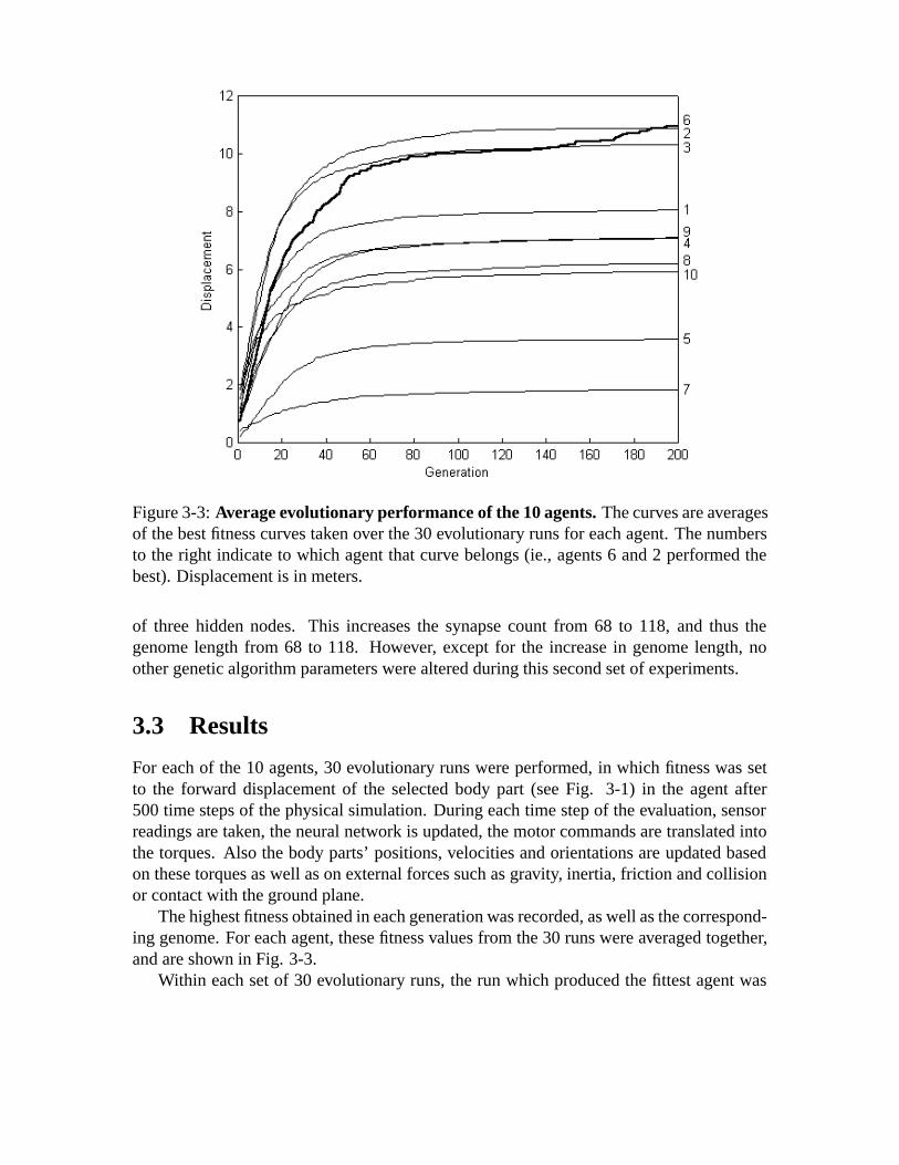
Figure 3-3:Average evolutionary performance of the 10 agents.The curves are averagesof the best fitness curves taken over the 30 evolutionary runs for each agent. The numbersto the right indicate to which agent that curve belongs (ie., agents 6 and 2 performed thebest). Displacement is in meters.

of three hidden nodes. This increases the synapse count from 68 to 118, and thus thegenome length from 68 to 118. However, except for the increase in genome length, noother genetic algorithm parameters were altered during this second set of experiments.

3.3 Results

For each of the 10 agents, 30 evolutionary runs were performed, in which fitness was setto the forward displacement of the selected body part (see Fig. 3-1) in the agent after500 time steps of the physical simulation. During each time step of the evaluation, sensorreadings are taken, the neural network is updated, the motor commands are translated intothe torques. Also the body parts’ positions, velocities and orientations are updated basedon these torques as well as on external forces such as gravity, inertia, friction and collisionor contact with the ground plane.

The highest fitness obtained in each generation was recorded, as well as the correspond-ing genome. For each agent, these fitness values from the 30 runs were averaged together,and are shown in Fig. 3-3.

Within each set of 30 evolutionary runs, the run which produced the fittest agent was

1

2

3

4

5

6

7

8

9

10

Figure 3-4:Footprint graphs produced by the most fit agent of each type.Numbersindicate agent index as given in Fig. 3-1. The horizontal axis indicates time; the rowsarranged along the vertical axis correspond to one of the body parts comprising the agentthat comes in contact with the ground plane for at least one time step during evaluation.Black bars indicate time periods for which the body part is in contact; the white gapsindicate periods in which it is not in contact with the ground plane.

found, and the time steps for which the agent’s body parts were in contact with the groundplane were recorded. The footprint graphs for these agents from each agent type are areshown in Fig. 3-4.

In order to account for the performance differences indicated in Fig. 3-3, various mor-phological aspects of the agents were compared against their average evolutionary perfor-mance. Average evolutionary performance was computed by collecting the best fitnessvalues achieved at the end of each of the 30 evolutionary runs, and averaging them. Fig. 3-5 plots the agent’s total mass against average evolutionary performance. Fig. 3-6 plots thenumber of points of contact of the agent with the ground plane against average evolutionaryperformance.

Finally, a second set of experiments was conducted in which the hidden layer was ex-panded from three neurons to five neurons. Thirty evolutionary runs were again performedfor each agent type, and the fittest genome was retained, and its fitness recorded, after eachgeneration. The best fitness achieved at the end of each run was recorded and averagedwithin the set of 30 runs, for each agent. Fig. 3-7 plots the performance increase (or

Figure 3-5: Mass versus evolutionary performance.The horizontal axis indicates thetotal mass of the agent, in kilograms. The vertical axis indicates the average displacementof the targetted body part for each agent type, in meters. The numbers above the barsindicate the agent index as given in Fig. 3-1. The error bars are two standard deviationunits in length.

decrease) for each agent type realized by the increase in neural network size.

3.4 Discussion

Fig. 3-4 shows that most of the agents achieve a relatively rhythmic gait during evolution,with the exception of the segmented agent 5. For example, the tripedal agent (agent 10)keeps its left and right feet on the ground plane while its central leg swings into the air, andwith the aid of the momentum of the return stroke falls into a regular gait where the leftand right legs move in almost perfect synchrony (lowest panel, Fig. 3-4).

As can be seen from Fig. 3-3, it is much easier to evolve locomotion for two of the

Figure 3-6: Points of contact versus evolutionary performance.The horizontal axisindicates how many body parts of the agent can contact the ground plane. The vertical axisindicates the average displacement of the targetted body part for each agent type, in meters.The numbers above the bars indicate the agent index as given in Fig. 3-1. The error barsare two standard deviation units in length.

quadrupedal agents (agents 2 and 3) and the hexapedal agent (agent 6) using the genetic al-gorithm and neural network architecture reported here, than is the evolution of locomotionfor the segmented agents (agents 5 and 7). Because the evolutionary method and neuralcontrollers were kept constant for all agents, a morphological explanation must be found toaccount for this performance discrepancy.

One hypothesis is that the greater the number of legs an agent has, the more difficult itis to evolve a neural controller to coordinate them, or they generate more friction with theground, and thus make locomotion more difficult.

However, Fig. 3-6 seems to refute this hypothesis, as there seems to be an inverseU-shape relationship between performance and leg number: performance increases fromthe tripedal agent (agent 10) up to the hexapedal agent, and then decreases again as the

Figure 3-7:Change in performance based on addition of hidden neurons.The lightcoloured bars indicate the average evolutionary performance for that agent using three hid-den neurons. The dark coloured bars indicate average performance for that agent using fivehidden neurons. Numbers along the horizontal axis denote the agent’s index number, asdenoted in Fig. 3-1. The error bars are two standard deviation units in length.

number of points of contact increases. This may be a general trend, and needs to be testedby including more agents in the group, such as bipedal and octapedal agents.

An alternative hypothesis is that the segmented agents have larger masses, and becausethe number of motors and the torque ceiling is kept constant across agents, it may simplybe more difficult for the heavier agents to locomote. This hypothesis seems to be supportedby the data reported in Fig. 3-5, because there is a partial negative correlation betweenmass and evolutionary performance. However, the three best agents (agents 2, 3 and 6) runagainst this apparent correlation, suggesting that mass is a necessary, but not a sufficientmorphological explanation for the observed performance differences, and that six legs maybe an optimal configuration for this experimental setup. We can envisage several othermorphological explanations that could be tested using this method: static stability, dynamicstability, and orientation of joints are just a few possibilities.

Aside from isolating and testing hypotheses about specific morphological characteris-tics, by experimenting with sets of agents instead of just a single agent, we can measurethe general effect of controller and evolutionary method choices, not just how they affecta particular agent. For example, Fig. 3-7 shows that by increasing the size of the neuralnetwork by adding hidden neurons is a great advantage for the segmented agents with manysimilar parts, helps somewhat with the other agents, but has no significant advantage for

Figure 3-8:The best evolved gaits using two different neural networks.The upper panelshows the best evolved gait for agent 5 using a hidden layer with three neurons. The lowerpanel shows the best evolved gait for the same agent using a hidden layer with five neurons.

the tripedal agent. The advantage for the segmented agents is made more clear in Fig. 3-8,where the best evolved gait for agent 5 using three hidden neurons is contrasted againstthe best evolved gait using five hidden neurons. The first gait allowed the agent to travel2.45 meters in 500 time steps; the second gait allowed the agent to travel 7.58 meters. Itcan be seen that in the first case the best gait has not yet achieved rhythmicity, whereasthe second gait is much more rhythmic. Note also that despite hand-tuning the maximummotor torques, the second gait has achieved jumping: there are periods of time for whichno part of the agent is in contact with the ground plane.

The large performance increase observed for the segmented agents lends support to thehypothesis that segmented animals require multiple, modular neural components in orderto achieve travelling waves of muscular contraction in order to move [Ijspeert and Kod-jabachian, 1999]. Our result also agrees with that of Gruau [Gruau and Quatramaran, 1996],who reported that a neural network with 16 hidden nodes was required, in his experimentalsetup, to evolve locomotion for an eight-legged robot.

By comparing new evolutionary techniques and controller architectures on differentagents, it is possible to determine whether any observed gain in performance is general, oris useful only for particular agents. For example in this paper we have demonstrated thatincreasing network size is useful for segmented agents, but not for the tripedal agent. Wehypothesize that if the triped, which is inherently unstable, were equipped with tilt sensorsit may be possible to exploit the extra neural connections for balanced locomotion.

3.5 Conclusions

In this paper we have introduced a comparative methodology that serves two purposes.First, it can be used to measure how much a particular morphological characteristic willfacilitate or hamper the evolution of behaviours for simulated agents. Moreover, becausethe methodology encompasses a group of agents, it could allow for predictions as to howeasy or difficult it will be to evolve the behaviours for new agents, if the new agent sharesone of the morphological characteristics with an agent from the original group. For ex-ample, because we have found that quadrupeds and hexapods are particularly good candi-dates for which to evolve locomotion, given our choice of neural network and evolutionaryscheme, we predict that it would be relatively easy to evolve locomotion for new agents

with quadupedal or hexapedal body plans.Second, by modifying the evolutionary scheme or controller, re-evolving the agents in

the set for the same behaviour, and then measuring performance changes, we can begin tounderstand how particular controller architectures or evolutionary schemes are appropriate—or inappropriate—for particular agents.

As physical simulation becomes more sophisticated and computational power continuesto increase, it has become feasible to test hypotheses about adaptive behaviour on a wholeclass of agents, not just a single instantiation. Moreover, by gaining more specific insightsinto morphological effects on behaviour, it may become easier to transfer evolved agentsfrom physical simulation to real world robots.

Chapter 4

Making Evolution an Offer It Can’t Refuse:Morphology and the Extradimensional Bypass1

Abstract

In this paper, locomotion of a biped robot operating in a physics-based virtual environmentis evolved using a genetic algorithm, in which some of the morphological and controlparameters of the system are under evolutionary control. It is shown that stable walkingis achieved through coupled optimization of both the controller and the mass ratios andmass distributions of the biped. It was found that although the size of the search space islarger in the case of coupled evolution of morphology and control, these evolutionary runsoutperform other runs in which only the biped controller is evolved. We argue that thisperformance increase is attributable to extradimensional bypasses, which can be visualizedas adaptive ridges in the fitness landscape that connect otherwise separated, sub-optimaladaptive peaks. In a similar study, a different set of morphological parameters are includedin the evolutionary process. In this case, no significant improvement is gained by coupledevolution. These results demonstrate that the inclusion of the correct set of morphologicalparameters improves the evolution of adaptive behaviour in simulated agents.

4.1 Introduction

In the field of robotics, much work has been done on optimizing controllers for bipedrobots [Benbrahim and Franklin, 1997, Kun and Miller, 1996, Vukobratovic, 1990]. Simi-larly, genetic programming [Gruau and Quatramaran, 1996] and genetic algorithms [Gal-lagher et al., 1996] have been used to evolve controllers for hexapod robots. Genetic al-gorithms have also been used to evolve recurrent neural networks for bipedal locomotion:Fukudaet al[1997] employed a dynamic simulator; Reil and Husbands [Reil and Husbands, 2002]

1Appeared as Bongard, J. C. & C. Paul, “Making Evolution an Offer It Can’t Refuse: Morphology and theExtradimensional Bypass”, in J. Keleman & P. Sosik (eds.),Proceedings of the Sixth European Conferenceon Artificial Life, Springer-Verlag, pp. 401-412, 2001.

40

employed a three-dimensional physics-based simulator. However, in all of these approaches,little or no consideration was paid to the mechanical construction of the agent or robot.

Alternatively, Brooks and Stein [Brooks and Stein, 1994] and Pfeifer and Scheier [1999]have pointed to the strong interdependence between the morphology and control of an em-bodied agent: design decisions regarding either aspect of an agent strongly bias the re-sulting behaviour. One implication of this interdependence is that often, a good choice ofmorphology can lead to a reduction in the size or complexity of the controller. For example,Lichtensteiger and Eggenberger [Lichtensteiger and Eggenberger, 1999] demonstrated thatan evolutionary algorithm can optimize the sensor distribution of a mobile robot for certaintasks, while the controller remains fixed. As an extreme case, the study of passive dynam-ics has made clear that a careful choice of morphology can lead to locomotion without anyactuation or controller at all [McGeer, 1990].

Examples now abound that demonstrate that the evolution of both the morphology andcontrol of simulated agents [Sims, 1994, Ventrella, 1994, Adamatzky et al., 2000, Chocronand Bidaud, 1999, Mautner and Belew, 1999], as well as real-world robots [Lund et al.,1997, Juárez-Guerrero et al., 1998, Lipson and Pollack, 2000] is possible. However, weargue in [Bongard and Paul, 2000] that the coupled evolution of both morphology and con-trol of adaptive agents is not as interesting in and of itself: rather, the implications of suchstudies open up a host of research questions regarding the evolution of adaptive behaviourthat are not amenable to study solely through the optimization of control. Virtual EmbodiedEvolution (VEE) was introduced in [Bongard and Paul, 2000] as a systematic methodologyfor investigating the implications of evolving both the morphology and control of embodiedagents. In this paper we show not only that coupled evolution of both morphological andcontrol parameters of a bipedal agent can facilitate the discovery of stable locomotion—despite the increased size of the search space necessitated by the inclusion of the additionalmorphological parameters—but also that only certain sets of morphological parameters fa-cilitate evolutionary search.

The following section introduces the mechanical construction and neural controller ofthe biped agent, as well as the genetic algorithm used to evolve locomotion. Section 4.3presents the results obtained from evolving only the neural networks for a bipedal agent, aswell as evolutionary runs in which morphological parameters were included in the genome.Section 4.4 provides some discussion and analysis as to why coupled evolution of morphol-ogy and control can outperform the evolution of control. In the final section we concludeby stressing the importance of incorporating morphological considerations into the evolu-tionary investigation of adaptive behaviour.

a) b) c)M 1 M 2 M 3 M 4 M 5 M 6

T1 T2 P1 P2 P3 P4 P5 P6 B1

B2

OUTPUT LAYER

INPUT LAYER

HIDDEN LAYER

Figure 4-1:Agent construction and neural network topology.a) shows the biped agentwithout the attached masses. b) shows the agent with the attached masses. c) gives apictorial representation the neural network used to control both types of agents.T1 andT2correspond to the two touch sensors,P1 throughP6 indicate the six proprioceptive sensors,andM1 throughM6 indicate the six torsional motors of the biped.B1 andB2 indicate thetwo bias neurons.

4.2 The Model

For all of the evolutionary runs reported in this paper, the agents act within a physically-realistic, three-dimensional virtual environment2. The agent is a simulation of a five-linkbiped robot with six degrees of freedom. The agent has a waist, and two upper and lowerleg links as shown in Fig. 4-1 a). Each knee joint, connecting the upper and lower leg links,has one degree of freedom in the sagittal plane. Each hip joint, connecting the upper leg tothe waist, has two degrees of freedom: one in the sagittal plane and one in the frontal plane.These correspond to the roll and pitch motions. In the second set of experiments reportedin section 4.3, a second type of biped is used, in which five mass blocks are attached to thelower legs, upper legs and waist as shown in Fig. 4-1 b).

The joints are limited in their motion using joint stops, with ranges of motion closelyresembling those of human walking. The hip roll joint on each side has a range of motionbetween−π

7and π

7radians with respect to the vertical. The hip pitch joint has a range of

motion between− π10

and π10

, also with respect to the vertical. The knee joint has a rangeof motion between−π

2and0 with respect to the axis of the upper leg link to which it is

attached. Table 4.1 summarizes the morphological parameters for both types of bipeds.The agent contains two haptic sensors in the feet, and six proprioceptive sensors and

torsional actuators attached to the six joints, as outlined in Figs. 4-1 a) and b). At each

2The environment and biped agents were constructed and evaluated using the real-time physics-basedsimulation package produced by MathEngine PLC, Oxford, UK,www.mathengine.com.

Table 4.1:The default size dimensions, masses and joint limits of the biped.Parametersset in boldface indicate those parameters that are modified by evolution in the experimentsreported in section 4.3. The valid ranges for these parameters are also given.

Index Object Dimensions Mass

1 Knees r = 1ul 1um each2 Hip sockets r = 1ul 1um each3 Feet r = 2ul, w = 3ul 1um each4 Lower Legs r = [0.2,0.8] ul, h = 8ul 0.25um each5 Upper Legs r = [0.2,0.8] ul, h = 8ul 0.25um each6 Waist r = [0.2,0.8] ul, w = 8ul 0.25um7 Waist Block l = [0.4,3.6] ul, w = h = [0.2,3.0] ul 0.103um8 Lower Blocks l = [0.4,3.6] ul, w = h = [0.2,3.0] ul 0.103um each9 Upper Blocks l = w = [0.2,3.0] ul, h = [0.4,3.6] ul 0.103um each

Index Joint Plane of Rotation Range (rads)

10 Knee sagittal −π2→ 0

11 Hip sagittal −π7→ π

7

12 Hip frontal − π10→ π

10

time step of the simulation, agent action is generated by the propagation of sensory inputthrough a recurrent neural network; the values of the output layer are fed into the actuatorsas desired positions. The input layer contains nine neurons, with eight corresponding to thesensors, and an additional bias neuron. All neurons in the network emit a signal between−1 and1: the haptic sensors output1 if the foot is in contact with the ground, and−1otherwise; the proprioceptive sensor values are scaled to the range[−1, 1] depending ontheir corresponding joint’s range of motion; and bias neurons emit a constant signal of1.The input layer is fully connected to a hidden layer composed of three neurons. The hiddenlayer is fully and recurrently connected, plus an additional bias neuron. The hidden and biasneurons are fully connected to the eight neurons in the output layer. Neuron activations arescaled by the threshold function2

1+e−a − 1. The values at the output layer are scaled to fitthe range of their corresponding joint’s range of motion. Torsion is then applied at eachjoint to attain the desired joint angle.

Evolution of bipedal locomotion is achieved using a floating-point, fixed-length geneticalgorithm. Each genome encodes weights for the60 synapses in the neural network, plusany additional morphological parameters. All values in the genome range between−1.00and1.00. Each evolutionary run reported in this section is performed using a populationsize of300, and is run for300 generations. Strong elitism is employed in which150 ofthe most fit genotypes are preserved into the next generation. Tournament selection, witha tournament size of three, is employed to select genotypes from among this group formutation and crossover.38 pairwise one-point crossings produce76 new genotypes. The

remaining74 new genotypes are mutated copies of genotypes from the previous generation:an average of five point mutations are introduced into each of these new genotypes, usingrandom replacement.

In the set of experiments using the agent shown in Fig. 4-1 a), three additional mor-phological parameters are included in the genome. These parameters dictate the radii ofthe lower legs, upper legs and waist, respectively. The range of possible radii for thesesegments is[0.2, 0.8] unit length3 In the second set of experiments, eight morphologicalparameters are included in the genome: the first three values dictate the widths of the lowermass block pair, upper mass block pair and waist mass block, respectively, each of whichcan range between0.2 and3.0 ul. The next three values indicate the lengths of the lowermass block pair, upper mass block pair and waist mass block, respectively, which rangebetween0.4 and3.6 ul. The final two values indicate the vertical placement of the lowerand upper block mass pairs, which can range between0.8 to 7.2 ul above the centre of thefoot: in this way, all four blocks can be attached to the upper or lower pairs of legs. Thehorizontal position of the waist block mass remains centred, and is not changed. In the caseof agents without block masses, the morphological parameter settings can affect the massdistribution and moment of inertia of the agent. In the case of agents with block masses,the morphological parameter values can also affect the mass distribution and the momentof inertia, although more degrees of freedom of the rotational moment of inertia are subjectto selection pressure in this case. For the variable morphology evolutionary runs, the threeor eight morphological parameters are distributed evenly across the length of the genomein order to maximize recombination of these values during crossover.

The fitness of a genome is determined as follows. The weights encoded in the genotypeare assigned to the synapses in the neural network, and in the case of the variable mor-phology bipeds without mass blocks, the radii of the waist, lower and upper legs are setbased on the additional three values in the genome. In the case of the variable morphologybipeds with the mass blocks, the dimensions and positions of the blocks are set based onthe additional eight parameters. The agent is then evaluated for up to 2000 time steps inthe physical simulator. Evaluation halts prematurely if both of the feet leave the groundat the same time (this discourages the evolution of running gaits); the height of the waistpasses below the height of the knees; or the waist twists more than 90 degrees away fromthe desired direction of travel. The northern distance of the agent’s hip at the terminationof the evaluation period is then treated as the fitness of the genome.

4.3 Results

Four sets of evolutionary runs were conducted using the parameters given in Table 4.2. Fig.4-2 summarizes the evolutionary performance of the two sets of runs using agents withoutmass blocks, and Fig. 4-3 reports the evolutionary performance of the two sets of runs

3All lengths and masses reported in this paper are relational: the unit length (ul), and the default mass(um), are set equal to the radii and masses of the knee and hip sockets, respectively.

Table 4.2:Experimental regime summary.Run Morphology Blocks Total Genome Number ofSet block mass length independent runs

1 Fixed Absent N/A 60 302 Variable Absent N/A 63 303 Fixed Present 0.512um 60 204 Variable Present 0.512um 68 20

a) b)

c) d)

Figure 4-2:Evolutionary performance of fixed and variable morphology agent popu-lations without mass blocks.a) and b) report the highest fitness values attained by agentswith fixed and variable morphologies, respectively, from 30 independently evolving popu-lations of each agent type. c) and d) report the average fitness of these populations.

using agent populations with mass blocks. It can be seen in Fig. 4-2 that in both fixed andvariable morphology agent populations, there is a roughly uniform distribution of fitnessperformance achieved by the most fit agents at the end of the runs. However Figs. 4-2b) and d) indicate that variable morphology populations repeatedly achieved higher fitness

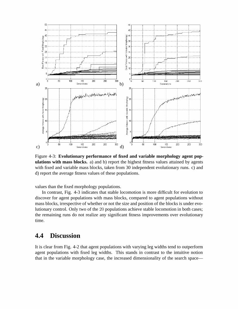
a) b)

c) d)

Figure 4-3:Evolutionary performance of fixed and variable morphology agent pop-ulations with mass blocks.a) and b) report the highest fitness values attained by agentswith fixed and variable mass blocks, taken from 30 independent evolutionary runs. c) andd) report the average fitness values of these populations.

values than the fixed morphology populations.In contrast, Fig. 4-3 indicates that stable locomotion is more difficult for evolution to

discover for agent populations with mass blocks, compared to agent populations withoutmass blocks, irrespective of whether or not the size and position of the blocks is under evo-lutionary control. Only two of the20 populations achieve stable locomotion in both cases;the remaining runs do not realize any significant fitness improvements over evolutionarytime.

4.4 Discussion

It is clear from Fig. 4-2 that agent populations with varying leg widths tend to outperformagent populations with fixed leg widths. This stands in contrast to the intuitive notionthat in the variable morphology case, the increased dimensionality of the search space—

Figure 4-4: Schematic representation of an extradimensional bypass.In the one-dimensional Euclidean fitness landscape indicated by the cross-section within the verticalplane, the adaptive peakA is separated by a wide gulf of low fitness phenotypes from thehigher peakB. In the higher dimensional fitness landscape indicated by the surface, anextradimensional bypass, represented by the curved surface, connects peaksA andB.

corresponding to the additional three morphological parameters—will degrade search.We did not find evidence that the variable morphology populations tended to converge

on any particular mass distribution. On the contrary, the morphological parameters ofthe most fit agents at the end of each run fall within their possible ranges with a roughlyuniform distribution. This suggests that for our particular instantiation of bipedal loco-motion and choice of controller, no one mass distribution is better than another. In otherwords, evolution of variable morphology agents does not perform better because evolutionis able to discover a “good” morphology: rather, the addition of morphological parameterstransforms the topology of the search space through which the evolving population moves,creating connections in the higher dimensional space between separated adaptive peaks inthe lower dimensional space. These connections are known as extradimensional bypasses,and were introduced by Conrad in [Conrad, 1990].

Using a Euclidean topology to represent a fitness landscape, the cross-section withinthe vertical plane in Fig. 4-4 indicates a one-dimensional landscape in which the value of asingle phenotypic traitP1 dictates fitnessF. This landscape contains two separated adaptivepeaks,A andB: a population centred around peakA cannot easily make the transitionto the higher fitness peak atB. However, through the addition of a second phenotypicparameterP2, the landscape is expanded to two dimensions (indicated by the surface), andan adaptive ridge—indicated by the upward sloping arrow—provides an opportunity for anevolving population to move from peakA to B via this extradimensional bypass. Using the

Euclidean space metaphor here has made it easy to visualize the way in which morphologyis exploited to improve evolution. However, the concept of an extra dimensional bypass canbe generalized to non-Euclidean representations of fitness topologies, such as the fitnessgraphs described in [Jakobi, 1996].

We hypothesize that although the additional morphological parameters increase the di-mensionality of the search space, in this case they introduce more adaptive ridges con-necting local adaptive peaks, and facilitating evolutionary search. In other words, givena particular morphology, any combination of control changes does not confer increasedfitness, but a change in morphology, coupled or followed by control changes does conferincreased fitness. This is supported by the variable morphology populations, some of whichdo not converge at the end of the evolutionary run on morphologies far removed from thedefault case.

More direct evidence for the presence of extradimensional bypasses has been found inadditional evolutionary runs, in which the genetic algorithm again optimizes the controlparameters and the leg widths of the simulated biped without mass blocks. In these runsthe population is seeded with random control parameters, but the three morphological pa-rameters in the genome are all set to the default leg width of0.5 unit length. Figs. 4-5 a)and b) report the morphological history of the best individuals from two successful evolu-tionary runs. Figs. 4-5 c) and d) report the corresponding best and average fitness of thetwo populations. The patterns of morphological change in these populations is typical ofthose found in the additional runs.

In both populations, the most fit individual at the end of the evolutionary run has a mor-phology identical or very similar to the starting, default case. These findings disprove thealternative hypothesis that search is improved when both the controller and morphologyare evolved because there is one or several morphologies that are better suited to locomo-tion than the arbitrarily chosen default configuration. In other words, the morphologicalparameters do not introduce new, high peaks in the fitness landscape that did not exist inthe lower dimensional space.

On the other hand, there are long periods in which the most fit individual has a morphol-ogy far removed from the default case. This indicates that the morphological parametersare useful for evolutionary search for this task, and are being incorporated into the fitterindividuals in the population. This indicates that the evolving population is moving alongthe extra dimensions introduced by the morphological parameters.

Both of these findings support the hypothesis that the additional morphological param-eters transform the fitness landscape to some degree, and allow for more rapid discovery ofstable bipedal locomotion. Moreover, Figs. 4-5 c) and d) show that several of the periodsdominated by agents with the non-default morphological parameter values (indicated bythe dark bands on the best fitness curves) are succeeded by rapid fitness increases. Futurephylogenetic studies are planned to investigate how the genetic material from these periodsare incorporated into the subsequent genotypes that confer increased fitness on the agent.

The evolving agent populations with affixed mass blocks, indicated in Fig. 4-3, presentsa much different picture. In these populations, the addition of eight morphological param-

a) b)

c) d)

Figure 4-5:Morphological change in two populations.a) and b) indicate the leg widthsfor the most fit agent from two evolving populations. c) and d) indicate the best fitnessand average fitness of these populations. The dark bands on the best fitness lines indicateperiods in which those agents have morphologies far removed from the default case.

eters does not improve evolutionary search. In the20 fixed morphology populations and20 variable morphology populations, only two instances of stable locomotion were discov-ered in each. It is clear that bipedal locomotion using agents with mass blocks, using ourexperimental set-up, is a more difficult task for the genetic algorithm, but the appearanceof stable walking indicates it is not impossible for either the fixed or variable morphologyregime to discover stable locomotion.

From our current experiments it is not clear why evolutionary search is not improvedin this case, but it seems likely that there are two factors hindering improvement in thevariable morphology populations. First, it seems plausible that the ruggedness of the lowerdimensional fitness landscape, in the case of agents with fixed blocks, is greater than in thelandscape for agents without mass blocks and fixed leg widths, because of the decreasedevolutionary performance shown in Figs. 4-3 a) and c), compared with the performanceshown in Figs. 4-2 a) and c). Second, the dimensionality of the search space for agent

populations with mass blocks increases from60 to 68, as compared with an increase ofonly 60 to 63 for agent populations without mass blocks.

4.5 Conclusions and Future Research Directions

In this paper, stable locomotion was evolved in embodied, bipedal agents acting withina three-dimensional, physically-realistic virtual environment. It has been demonstratedthat, for the case of locomotion in these agents, the subjugation of certain morphologicalparameters to evolutionary search increases the efficacy of the search process itself, despitethe increased size of the search space.

Preliminary evidence was provided which suggests that artificial evolution does not dobetter in the case of the variable morphology populations because it is able to discover bettermorphologies than those imposed in the fixed morphology populations, but rather becausethe type of parameters included in the search create adaptive ridges linking previouslyseparate adaptive peaks.

However, a control set of experiments was provided in which a different set of mor-phological parameters were included in the genomes of the evolving populations. In theseexperiments, there was no performance increase in the search ability of the genetic algo-rithm. This suggests that for the artificial evolution of adaptive behaviour, the arbitraryinclusion of morphological parameters does not always yield better results.

In future experiments we plan to conduct phylogenetic studies and adaptive walks toinvestigate in more detail how the inclusion of morphological parameters transforms thefitness landscape of the evolving populations. Moreover, we hope to formulate a systematicmethod for predicting which morphological parameters of embodied agents can augmentthe evolutionary discovery of adaptive behaviour.

Chapter 5

Investigating Morphological Symmetry andLocomotive Efficiency using Virtual Embodied Evolution1

Abstract

The recent convergence of real-time physics-based simulation tools, the growing field ofembodied cognitive science, and techniques for evolving complete agents has created anew methodology, which we refer to as Virtual Embodied Evolution. This methodologycan be used to explore a wide range of issues related to the interplay between morphologyand control in adaptive behaviour research. Here, we explore the intuitive, but previouslyexplicitly unexplored correlation between morphological symmetry and locomotive effi-ciency in mobile, simulated agents. By evolving the morphologies and control structuresof simulated agents using a genetic algorithm, it was found that agents with a higher de-gree of bilateral symmetry tended to exhibit greater locomotive efficiency than agents withless bilateral symmetry. This finding lends credence to the argument that for biologicalorganisms, natural selection may have preceded, and continues to supplement sexual se-lection pressure favouring morphological symmetry. We conclude by discussing the futurepossibilities of virtual embodied evolution.

5.1 Introduction

The field of embodied cognitive science has developed into a coherent conceptual frame-work for the advancement of embodied artificial intelligence [Pfeifer and Scheier, 1999,Thelen and Smith, 1994, Varela et al., 1991, Clark, 1998]. However, embodiment raisesnew research issues. Genetic and/or learning methods are often used for automating thegeneration of adaptive agents, and it is difficult and time-consuming to iteratively modifythe shape of, and sensor and effector placements on real-world robots [Mataric and Cliff, 1996].

1Appeared as Bongard, J. C. & C. Paul, “Investigating Morphological Symmetry and Locomotive Effi-ciency using Virtual Embodied Evolution”, in J.-A. Meyer et al (eds.),Proceedings of the Sixth InternationalConference on the Simulation of Adaptive Behaviour, pp. 420-429, 2000.

51

On the other hand, developing adaptive agents completely in simulation raises its own chal-lenges, such as effectively preserving observed behaviour of simulated agents when trans-ferred to real-world robots [Jakobi, 1997, Tokura et al., 2001]. One possibility for bridgingthe gap between simulation and the real world is by employing a physics-based simu-lation tool for investigating embodiment-related issues [Sims, 1994, Mataric et al., 1999,Terzopoulos et al., 1996, Hokkanen, 1999]. In this paper, the MathEngine physics-basedsimulation package2 is used to study the relationship between symmetric morphology andefficient locomotion in evolved agents.

The first attempt to evolve both the morphology and control structure of simulatedagents is reported in [Sims, 1994]: agents were evolved for a variety of tasks using a recur-sive, graph-based genetic algorithm. In [Terzopoulos et al., 1996], a learning algorithm isused to generate behaviours for fish with three-dimensional body plans, which can deformand locomote within a simulated, physics-based environment. Ventrella [Ventrella, 1994]also evolved morphologies for simulated agents using a genetic algorithm: initial attemptsto generate symmetric morphologies by using a fitness function based solely on locomotionwere not successful. Subsequent experiments built symmetry into the genotype to pheno-type mapping, so that evolved agents exhibited slight variations on an underlying bilaterallysymmetric body plan. However, this work did not investigate the locomotive efficiency ofthe evolved agents.

In biological studies, the positive correlation between morphological symmetry andlocomotive efficiency has been demonstrated indirectly: it has been shown that fluctuatingasymmetry (slight, random deviations from bilateral symmetry) can have an aerodynamiccost in bird species [Thomas, 1993, Balmford et al., 1993, Evans et al., 1994]. In a studyof the harpacticoid copepodT. californicus, which exhibits bilateral variation, it was foundthat genetic factors which influence relative limb size, in turn affecting locomotion, areexpressed on both sides of the animal equally [Palmer et al., 1993].

In the biological literature, there are only a few reports of large-scale morphologicalasymmetry [Norberg, 1977, Freeman and Lundelius, 1982, Govind, 1989, Bock and Marsh, 1991].It is interesting to note that none of these asymmetric features relate to locomotion.

In this paper, we report a positive correlation between bilateral symmetry and locomo-tive efficiency for agents evolved in a physics-based, virtual task environment. Agents areevolved using two different fitness functions: one that awards for directed locomotion andbilateral symmetry, and another that awards for directed locomotion and bilateral asymme-try. We compare the locomotive efficiencies of the two types of agents.

In the next section, we describe this task environment, details of the fitness function,the genetic encoding and parameters of the genetic algorithm. In Sect. 3 we discuss thequantitative measures used for detecting locomotive efficiency. In Sect. 4 we report ourresults; in Sect. 5 we discuss the implications of our findings; we conclude in Sect. 6with a discussion of the rich potential of this methodology for future studies into the in-terdependence of morphology and control in both simulation and for real-world embeddedsystems.

2MathEngine PLC, Oxford, UK,www.mathengine.com

a) b)

Figure 5-1: Morphologies of two evolved agents.Fig. a) shows the morphology of asymmetric agent schematically. Fig. b) shows the morphology of an asymmetric agent.

5.2 The Model

All of the agents reported here operate within a virtual, real-time physics-based environ-ment that simulates the dynamics of multiple bodies which are affected by gravity, in-ertia, torque, and other internal and external forces. The morphologies of the evolvedagents are treated as directed trees, similar to the agents reported in [Ventrella, 1994] and[Adamatzky et al., 2000]. Each agent is composed of a number of spherical units with iden-tical size and mass. The units are connected to each other with links of uniform length andno mass. Units can be connected to a maximum of six other units. Connections betweenunits are constrained to the six cardinal directions up, down, north, south, east and west.Fig. 5-1 shows the morphologies of two agents evolved for bilateral symmetry and bilateralasymmetry, respectively.

5.2.1 Control architecture

The control of the agents is achieved through a recurrent neural network. The networkis embedded within the agent’s morphology. Fig. 5-2 shows a typical neural network,which evolved in concert with the morphology of the agent shown in Fig. 5-1 b). Neuralconnections can be constructed between connected units; neural activation to distant unitscan be achieved by propagating a neural signal along the synapses of neighbouring units.The neurons within the network fall into three classes: sensor neurons; motor neurons,and internal neurons. During each time step of the simulation, each neuron sums its input,applies the sigmoid activation function 1

1+e−a − 0.5 (wherea is the summed activation tothe neuron), and places the result on its output synapse(s). These results are used when thenetwork is updated again at the next time step.

Figure 5-2:A typical embedded, evolved neural networkThis network was evolved tocontrol the agent shown in Fig. 5-1 b). The darker circlesF1 andF2 indicate the two typesof motor neurons. The lighter circlesR, A andC represent range, joint angle and contactsensors. The grey boxes represent internal neurons. The large circles represent morpho-logical units. The thin lines represent intra-unit connections. The thick lines representinter-unit connections. The weights of the connections are not shown for clarity.

Three types of sensor neurons are used here. Contact neurons emit a maximum positivesignal when the unit in which it is contained is in contact with the ground; otherwise,they emit a maximum negative signal. Proprioceptive neurons emit a signal commensuratewith the current joint angle between two links connecting the parent unit and two childunits; if the joint is rigid, or if the unit housing the neuron does not have two children,the neuron emits a zero signal. Range sensors emit a value inversely proportional to thedistance between the unit housing the neuron and the single external target object in theenvironment. The target is placed 10 units3 in the direction in which the agent shouldmove. Thus, if the agent moves towards the target, the distance between the agent andthe target will decrease, and the range sensors will emit a higher signal. By placing range

3A unit in our simulation is equal to the uniform distance between any two morphological units; all otherdistance measures in the simulation are relative to this unit.

Figure 5-3:The two types of joint actuation Figs. a) and b) illustrate the different jointscreated by the two types of motor neurons.

sensors in different units, an agent can use a combination of differing range values to orienttowards the target.

Two types of motor neurons are available for use by the agent. The presence of a motorneuron within a unit converts that unit into the central point of a hinge joint. The two motorneuron types correspond to the two kinds of hinge joints, with different axes of rotation(see Fig. 5-3).

Since the morphology is treated as a tree structure, only the first unit cannot contain mo-tor neurons. Each unit can contain at most one motor neuron. The hinge joints are actuatedusing virtual springs; the elasticity and damping constants are fixed for all the agents andtheir constituent joints. Outputs of the motor neurons dictate changes in the equilibrium po-sition of the virtual springs, leading to smooth motion of the hinges, irregardless of whetherthe motor neurons emit a smooth or discontinuous signal [Pratt and Williamson, 1995].

The internal neurons can be employed by the genetic algorithm to create mappings andpropagate signals between the sensor neuron inputs and the motor neuron outputs.

5.2.2 Genetic encoding

A variable-length genetic algorithm [Harvey, 1992] was used for evolving the agents. Byusing variable-length genomes, it is possible for selection pressure to evolve agents withincreasing or decreasing morphological size and control structure by increasing or decreas-ing genome length. Initial populations of the GA contain strings of 800 bits. Selectionpressure can increase this length up to a maximum of 2400 bits. Tournament selection isused with a tournament size proportional to the GA population. Mutation rate is propor-tional to the bit string length, and is tuned to perform, on average, one bit flip for each newgenome generated in the population. Elitism is employed by carrying the top 50 per cent ofthe population into the next generation. In contrast to a developmental encoding scheme,we use a completely explicit encoding, in which each unit, connection, neuron, synapseand synapse weight directly maps onto a unique set of bits. By using a recursive rule set

to grow structure, symmetric forms are more prevalent than asymmetric forms. This canbe observed in the agents reported in [Sims, 1994] and [Ventrella, 1994], the symmetricneural networks grown using cellular encoding [Gruau and Quatramaran, 1996], and thesymmetric structures generated by L-systems [Rozenberg and Salomaa, 1992]. Anothertype of developmental process, which does not contain recursive rule sets, also tends toproduce symmetric structures, due to the uniform spatial distribution of transcription fac-tors [Eggenberger, 1997].

The genome is treated as a string representation of an n-ary tree; this tree becomes themorphological frame of the agent as the read head traverses the genome. Each subset of thebit string then maps to a unit in the agent’s morphology. Within this subset is contained theinformation necessary for constructing the local network architecture within that unit, suchas the number and type of the neurons, their interconnecting synapses, and the weights ofthe synapses. This region also includes information for creating outgoing synapses thatconnect to neurons in neighbouring units. Fig. 5-4 demonstrates this mapping in moredetail.

The agent’s phenotype is constructed from its genotype as a read head moves linearlyalong the genome. Mutation or crossover sometimes adds additional bits to the end ofthe original genome which are not expressed. In such cases, the non-expressed bits areretained, in case subsequent modification reactivates this part of the genome. If genometruncation occurs instead, when the read head reaches the end of the genome, default valuesare supplied for the missing parameters.

5.2.3 The fitness functions

Two fitness functions are used in this report: the first awards for directed movement andbilateral symmetry; the other awards for directed movement and bilateral asymmetry. Theagent operates in the task environment for a specified number of simulation time steps; atthe end of the simulation, the northern distance from the origin of the agent’s southernmostunit is returned as the agent’s directed movement away from the origin4.

5.2.4 Measuring bilateral symmetry

The bilateral symmetry of an agent is determined using the following algorithm: the verticalplane which intersects the unit whose horizontal position is closest to the average horizontalpositions of all the units, is considered the plane of symmetry. The symmetry measure isthen given by

s =4pl

(2n− 1)− p− l,

4The southernmost unit of the agent is found by searching for the unit with a position vector containingthe minimum z-component; the value of this z-component then indicates how far north the agent was able tomove its trailing body part. This method for awarding directed movement eliminates the evolution of linear,passive agents, as was found in [Sims, 1994].

Figure 5-4:The genotype to phenotype mapping.The lefthand column shows the growthof the agent’s phenotype derived from the parsing of the genotype shown in the righthandcolumn. Figs a) to c) show the mapping from the original bit string to a decimal, baseten representation. Fig. d) shows the placement of genetic markers for the current unit’sneighbours: the first number after the start-of-unit marker indicates how many units willconnect to the current unit. Fig. e) shows the creation of internal neural structure for a unit.Fig. f) shows the attachment of a neighbouring unit to a parent unit. Figs. g), h) and i)show the detailed construction of neural structure. Fig. j) shows the final phenotype of theagent reached at the end of parsing.

wheren is the total number of units comprising the agent;2n − 1 is the total numberof units and links comprising the agent;p is the number of pairs of units lying outsidethe plane of symmetry, and are symmetric about that plane; andl is the number of pairsof links not contained in the plane of symmetry, and are symmetric about that plane. Itfollows from this that agents composed of pairs of units and links which are all symmetricabout the plane of symmetry attain a symmetry value of one; agents with decreasing pairsof symmetric units and links attain decreasing symmetry values; the minimum possiblevalue is zero. Agents composed of morphological units which all fall within the plane of

symmetry are given a symmetry value of zero, to avoid the evolution of two-dimensionalagents: it was found that such agents produce unrealistic movement, such as tumblingmotions completely within the vertical plane centred at the origin.

Thus, the two fitness functions used to evolve the agents reported here are given byds,andd(1 − s); the first awards for directed movement and bilateral symmetry; the secondawards for directed movement and bilateral asymmetry.

5.3 Efficiency of Transport Measures

In order to compare the efficiency of transport between the symmetric and asymmetricpopulations, efficiency measures are used which compare the populations along axes rep-resenting different aspects of efficient locomotion.

The abstract idea of locomotive economy can be conceptualized with respect to severaldifferent criteria. In biology there is a standard nomenclature for categorizing ideas relatedto economy based on what variables are used [Blake, 1991]. Efficiency is defined as per-formance with respect to an ideal, independent of the purpose of a task. For example, in thecontext of mechanics it is defined as the ratio of work or energy input to output. The otheris the termeffectivenessor competencyin performance [Full, 1991]. These definitions fo-cus on the physical nature of a process. Effectiveness is defined as a qualitative evaluationof how a mechanism is adapted to its function. It is a study of form, and physical traits.Perfection is defined as the 100% efficient performance. Optimality represents the bestperformance that can be achieved given a set of limiting circumstances.

For the comparison of efficiency of transport we use four different measures related tothese ideas, which together give us a robust basis for drawing qualitative conclusions aboutlocomotive differences.

5.3.1 Path Efficiency

In general terms, efficiency characterizes the performance of a system relative to an ideal,applied to a single process at a time. In our simulation, every agent takes a certain pathbetween pointA, its starting point, and pointB, its location at the end of the simulation.The most efficient way for the agent to travel this path is to follow the straight line betweenA andB. A more convoluted path between these two points indicates that the agent’slocomotion is less efficient. Thepath efficiency, as we define it, quantitatively representsthis efficiency measure. It is the ratio of the minimum distance between pointsA andBwith respect to the length of the agent’s actual path between these points:

P.E. =Dmin(A B)

Dreal(A B)

, where (5.1)

Dmin(A B) = || �AB||. (5.2)

If the agent’s actual path lies exactly on the straight line from the starting point to endpoint, P.E. is 1, which indicates that it is 100% efficient. The further its actual path divergesfrom this straight line, P.E. decreases and approaches 0.

In our simulations, each agent acts for a finite time period, which is constant acrosssimulations. However, some agents have a stochastic path with no finite periodicity, sothe calculation of the absolute path efficiency is only attainable as the simulation timeapproached infinity.

P.E.∗ = limx→∞

Dmin(A B)

Dreal(A B)

(5.3)

Our P.E. measure calculated in equation 1 is thus an approximation to this absolute ef-ficiency and we assume that our simulation time is large enough that P.E. is asymptoticallyapproaching the value P.E.∗. It has been empirically observed that our simulation time islarge enough to see large stable differences between agents’ locomotor trajectories, whichsupports our assumption.

5.3.2 Locomotive Effectiveness

Effectiveness is defined as a qualitative evaluation of how a mechanism is adapted to itspurpose or function. In our simulation the agents are evolved to make the greatest possibleprogress in the heading direction of the target, arbitrarily defined as North. Given thatthe most effective way to move towards the target is to travel exactly on the straight linebetween the starting point and the target locationT , theLocomotive Effectivenessquantifiesthe relationship between the agent’s actual path and distance moved in the target direction,as the ratio between these values.

L.E. =DNorth

Dreal(A B)

(5.4)

DNorth = �AB · �AT (5.5)

If the agent’s actual path lies exactly on the straight line from the starting point to the target,i.e. along vector�AT , the L.E. is 1, which indicates maximum effectiveness. The more itsactual path diverges from this straight line its L.E. value drops off.

5.3.3 Metabolic Efficiency

In robotics the integral over all the actuator forces represents the internal metabolic energyinput into the system. In our model, each of the joints is actuated by a virtual dampedtorsional spring with spring equation:

F = kθ − dθ (5.6)

wherek is the spring constant,d the damping constant, andθ the angular displacement ofthe spring from its equilibrium position.

The position of joint is controlled by the motor neurons which change the equilibriumposition of the joint. Thus at each time step the force applied on the arm is a function ofthe angular displacement between the natural angle valueθnat of the joints and its actualangle,θact.

The Total Metabolic Energy is a measure of the internal metabolic energy used by theagent to produce its entire sequence of motions. This can be calculated here as the integralover all the forces used by each joint, which is proportional to the

T.M.E. = (k

τ∫0

θact − θnat)− d(θτ − θ0) (5.7)

Since we will only be using the T.A.E as a relative measure we choosek = 1 for conve-nience sake.

In robotics, optimality of locomotion can be measured as the T.A.E, the simple integralover all the forces applied to each actuator, or as the T.A.E. value divided by the cycleperiod (given a periodic gait), or step length (for legged locomotion). Since our gaits maybe aperiodic and without clearly identifiable steps, we use the measure of the T.A.E. valuedivided by the distance travelled in the target direction,DNorth.

M.E. =T.M.E

DNorth(5.8)

This gives us an efficiency measure in terms of energy used per unit distance and en-ables us to concretely compare the energy usage of agents with equal fitness.

5.4 Results

A total of 10 runs were performed, for300 generations each, and using a population sizeof 300. When an agent was constructed from a bit string, it was allowed to act within thephysics-based environment for20, 000 time steps. Five of the runs used the fitness functionds, and the other five usedd(1 − s), whered ands are described in the previous section.At the end of each run, the five most fit, unique agents were extracted from each run, andaspects of their locomotive efficiency was measured.

It was found that the genetic algorithm rapidly converges to almost completely bilater-ally symmetric (s approaches1.0) or asymmetric (s approaches0.0) agents, depending onthe fitness function used. For this reason, it was possible to classify the extracted agents intotwo distinct classes, a symmetric and an asymmetric class. Fig. 5-5 shows the behaviour ofone completely bilaterally symmetric agent that was evolved. Fig. 5-6 shows the behaviourof an asymmetric agent. Both agents had similar fitness values. The morphologies for theseagents are shown in Figs. 5-1 a) and b), respectively. For each evolved agent, the trajectory

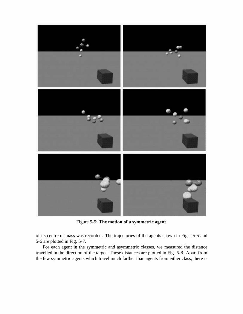
Figure 5-5:The motion of a symmetric agent

of its centre of mass was recorded. The trajectories of the agents shown in Figs. 5-5 and5-6 are plotted in Fig. 5-7.

For each agent in the symmetric and asymmetric classes, we measured the distancetravelled in the direction of the target. These distances are plotted in Fig. 5-8. Apart fromthe few symmetric agents which travel much farther than agents from either class, there is

Figure 5-6:The motion of an asymmetric agent

no significant difference in distance travelled.Within each class, the agents were then grouped according to fitness, andDreal was

computed for each agent, using the starting point of the agent’s centre of mass as pointA,and the final point of its centre of mass as pointB. The actual distance the agent travelsbetweenA andB is then calculated by summing the distance travelled by its centre ofmass during each time step of the simulation. TheDreal values were then averaged within

a) b)

Figure 5-7: Trajectories for a symmetric and an asymmetric agent. Trajectories aremeasured as changes in the agent’s centre of mass over the length of the simulation. Theactual trajectories are shown using a thick line; the corresponding distance fromA to Bare drawn with a thin line. Note that both agents move a similar distance north, implyingsimilar fitness values.

Figure 5-8:Distances travelled by symmetric and asymmetric agents

each group of similar fit agents, for both the groups of symmetric and asymmetric agents.The resulting averages are shown in Fig. 5-9. The metabolic efficiency of each agent wascalculated, using Eqn. 5.8. Agents were then grouped according to symmetry, and similarvalues forM.E. The numbers of agents falling within these groups are shown in Fig. 5-10.

Figure 5-9:Differences in average, actual distance travelled by similarly fit symmetricand asymmetric agents.

The path efficiency of each agent P.E. (see Eqn. 5.1) was calculated. Differences be-tween the path efficiencies of the symmetric and asymmetric agents are plotted againstfitness in Fig. 5-11.

5.5 Discussion

5.5.1 Symmetry and Efficiency

By observing the behaviours of many bilaterally symmetric and asymmetric agents, it be-comes clear that the movement of asymmetric agents is almost always more erratic forasymmetric agents. The trajectories of two agents—one completely bilaterally symmetric,the other completely bilaterally asymmetric—are shown in Fig. 5-7. The morphologies ofthe two agents are shown in Fig. 5-1. The relative eccentricity of the asymmetric agent’s

Figure 5-10:Differences in metabolic efficiency between symmetric and asymmetricagents.Note that thex-axis uses 1

M.E, so that agents near they-axis have higher metabolic

efficiency than agents grouped further from they-axis.

trajectory is evident from its greater deviation from the correspondingDmin vector.A general trend towards greater path eccentricity for asymmetric as opposed to sym-

metric agents is shown by Fig. 5-9. For agents that travel a similar distance in the directionof the target, asymmetric agents tend to travel a further distance to reach the directed dis-tance than the corresponding symmetric agents. Fig. 5-11 shows a similar result, wherethe distance travelled in the direction of the target is replaced by the line-of-flight vectorfrom the agent’s starting point to its ending point. Again, it was found that for agents withsimilar distances between their starting and ending points, asymmetric agents tend to travelfurther to achieve this distance than the corresponding symmetric agents.

In addition to path inefficiency, asymmetric agents were found to be more metabolicallyinefficient than symmetric agents, as is shown in Fig. 5-10. For agents which move similardistances in the direction of the target, asymmetric agents tend to apply more total force totheir actuators than corresponding symmetric agents.

Figure 5-11:Path efficiencies for symmetric and asymmetric agents.

Bilateral symmetry in biological organisms is believed to have evolved only once, andhas become a permanent feature of most higher animal species. However, why bilateralsymmetry evolved initially is not well understood [Palmer, 1996]. Also, although the preva-lence of sexual selection for symmetry is widely documented [Enquist and Arak, 1994,Watson and Thornhill, 1994, Brookes and Pomiankowski, 1994], the origins of sexual se-lection for symmetry are not well explained. Our results suggest that natural selection forefficiency may be a common cause underlying both the evolution of bilateral symmetry andthe origin of sexual selection for symmetry.

Initial, random variations in bilateral symmetry may have given slightly more symmet-ric males an evolutionary advantage due to increased locomotive or metabolic efficency.Coupled with an initial, slight variation in female preference for symmetry, the offspringwould be symmetric, and the female offspring would be both symmetric and have a highermating preference for symmetry. Again, because symmetry implies efficiency, these sym-metric females would have a selective advantage over less symmetric females and wouldmate more. This leads to sexual selection for symmetry: positive feedback over subse-

quent generations causes morphological symmetry and sexual preference for symmetry tosaturate the population. In addition, due to the mechanics of sexual selection, both thepreference for symmetry, and symmetry itself would become more exaggerated.

Apart from the biological implications, this work also contributes to design principlesfor building mobile robots. These findings support the intuition that in order to achievedirectional fidelity a robot must have a near symmetric morphology. In addition, theyalso illuminate the less intuitive, latent correlation between symmetric morphologies andenergy efficient locomotion. By making this correlation explicit, this work contributes tothe central issues of efficiency in robotics research.

5.5.2 Morphology and Control Tradeoffs

Several observations of different agents’ locomotion patterns have revealed that some agentsexploit the physics for movement more than others. For example, many agents were ob-served to be statically unstable. These agents begin their movement by building on the mo-mentum generated by falling forward. Others were observed to accelerate a passive jointin a forward direction by actuating a distant joint. The behaviours are reminiscent of thetechniques collectively referred to as passive dynamic control in robotics [McGeer, 1990].

For this reason, it is not possible to derive a positive correlation between path andmetabolic efficiency. For example, in some cases an agent with a very high path efficiencymay be metabolically inefficient because it actuates all of its limbs over the length of thesimulation. In contrast, another agent with low path efficiency may only actuate its limbsfor a small fraction of the trajectory leaving the rest to physics, thereby achieving highmetabolic efficiency with passive dynamics. How evolved agents exploit passive dynamicsis a promising topic for future research.

Evolution is able to achieve this exploitation by tuning the agent’s morphology to thetask. For example, for a majority of the evolved agents with rich locomotive behaviours,the motor neurons were observed to only emit a constant signal over the length of thesimulation. This is a clear example of how morphological adaptations can lead to reducedcontrol complexity.

There are at least two distinct types of morphology and control tradeoffs. A controllermay exploit the physical characteristics of its morphology, such as damped springs, tocreate motions which do not need to be explicitly specified by the control architecture. Orthe control may exploit the environment as a means to communicate between different partsof its morphology reducing the need for internal communication in the control structure[Cruse et al., 1996].

5.5.3 Virtual Embodied Evolution

By evolving agents in a physics-based environment, it is possible to generate agents whichare more situated and embodied than agents evolved in more abstract environments. Also,because of the increased fidelity of the simulationvis a visthe real world, it is easier to

transport evolved designs to the real world while retaining the observed behaviour [Funesand Pollack, 1999]. Therefore, it remains possible to generate and test a large number ofdiffering body plans and related control structure completely in simulation. We refer to thismethodology as Virtual Embodied Evolution.

Although some studies have reported the evolution of complete, functioning agents in aphysics-based environment [Sims, 1994, Ventrella, 1994], these studies have served moreas proof-of-concept investigations: several assumptions and ‘tweaks’ were built into theneural circuitry, genotype/phenotype mapping or morphological form in order to reducethe computational requirements, or to evolve more ‘realistic’ agents.

However, with the advent of commercially available physics-based simulation tools,and the continued advances in personal computer power and speed, it is now possible to useVirtual Embodied Evolution to further the maturation of concepts related to embodimentin adaptive behaviour research. This paper has investigated one such concept, namely therelationship between morphological symmetry and locomotive efficiency in evolved agents.

There are a host of other research questions that can be pursued with Virtual EmbodiedEvolution: some examples might include whether allowing selection pressure to evolvecentral pattern generators leads to more efficient locomotion in the resulting agents; whattask environments favour (or discourage) the evolution of centralized neural structure; orhow the addition of various developmental mechanisms to an explicit genotype/phenotypemapping (such as the one presented here) affect the convergence to fit agents in the geneticalgorithm.

5.6 Conclusion

Through the use of an explicit genotype/phenotype mapping, which does not implicitlyfavour either morphological or control symmetries, distinct sets of bilaterally symmetricand asymmetry agents were evolved by using two fitness functions, one which awards forlocomotion and symmetry, and the other for locomotion and asymmetry. It was then shown,by comparing a suite of efficiency measures against morphological symmetry, that evolvedagents with relatively high bilateral symmetry tend to move more efficiently than highlyasymmetric agents.

The result that bilateral symmetry leads to locomotive and metabolic efficiency in theevolved agents reported here suggests that there may be a common cause underlying theevolution of bilateral symmetry and sexual selection for symmetry. It is hoped that thiswork will lead to more biological investigations into these issues.

This work has made explicit the connections between physics-based simulation, in-creased computing power, the maturation of concepts in embodied cognitive science, andevolutionary techniques. This confluence of ideas is referred to as Virtual Embodied Evo-lution, which represents a unique methodology for studying adaptive behaviour.

Chapter 6

Repeated Structure and Dissociation of Genotypicand Phenotypic Complexity in Artificial Ontogeny1

Abstract

In this paper, a minimal model of ontogenetic development, combined with differentialgene expression and a genetic algorithm, is used to evolve both the morphology and neuralcontrol of agents that perform a block-pushing task in a physically-realistic, virtual envi-ronment. We refer to this methodology as artificial ontogeny (AO). It is demonstrated thatevolved genetic regulatory networks in AO give rise to hierarchical, repeated phenotypicstructures. Moreover, it is shown that the indirect genotype to phenotype mapping resultsin a dissociation between the information content in the genome, and the complexity of theevolved agent. It is argued that these findings support the claim that artificial ontogeny is auseful design tool for the evolutionary design of virtual agents and real-world robots.

6.1 Introduction

In the field of evolutionary robotics and artificial life, emphasis is increasingly coming tobear on the question of evolvability: that is, how well the artificial evolutionary system con-tinually discovers agents or robots better adapted to the task at hand ([Wagner and Altenberg, 1996],[Kirschner and Gerhart, 1998]). It is becoming apparent that modularity, at either the ge-netic or phenotypic level, or both, is a desirable characteristic for attaining highly evolvablesystems ([Wagner, 1995, Rotaru-Varga, 1999, Calabretta et al., 2000]).

Developmental geneticists have made clear that evolved genetic regulatory networksin biological DNA contain master control switch genes, known asHox genes, which or-chestrate the transcription of other genes to grow high-level repeated structure, such as the

1Appeared as Bongard, J. C. & R. Pfeifer, “Repeated Structure and Dissociation of Genotypic and Phe-notypic Complexity in Artificial Ontogeny”, in Spector, L. et al (eds.),Proceedings of The Genetic andEvolutionary Computation Conference (GECCO-2001). San Francisco, CA: Morgan Kaufmann publishers,pp. 829-836, 2001

69

segments inD. melanogaster(refer to [Gehring and Ruddle, 1998] for an overview). It hasbeen shown in a dramatic set of experiments [Lewis, 1978] that mutations ofHoxgenes canlead to large-scale but localized changes in phenotype. It has been argued [Raff, 1996] thatin some cases, differentiation and/or duplication of a feature may allow evolution to co-opt one copy of the feature to perform a different functional role. This process is known asexaptation [Gould and Vrba, 1982]. A similar mechanism has been shown to have occurredat the gene level (see [Ohno, 1970]).

Riedl [Riedl, 1978] demonstrated that the information content of a complex organism2

is many orders of magnitude higher than that contained in the genome, and has argued thatthe increased complexity arises from the hierarchical organization of organic units.

Raff [Raff, 1996] has pointed out the same principle holds for the complex processesthat take place during ontogeny. Others have argued [Delleart and Beer, 1994] that an in-direct, developmental genotype to phenotype mapping allows for artificial evolution to dis-cover more complex phenotypes than is possible with direct mappings.

In this paper we introduce an augmented genetic algorithm, in which the genomes aretreated as genetic regulatory networks. The changing expression patterns of these net-works over time leads to the growth of both the morphology and neural control of a multi-unit, articulated agent, starting from a single unit. We refer to this system as artificialontogeny (AO), and as is shown in [Bongard and Pfeifer, 2003], such a system can be usedto evolve agents that perform non-trivial behaviours in a physically-realistic, virtual envi-ronment, such as directed locomotion in a noisy environment. It is reported here that inagents evolved for a block-pushing task, the morphologies exhibit hierarchical, repeatedstructure. Evolved agents from previous studies contain repeated structure, however thesestudies relied on more direct, parametric encoding schemes ([Sims, 1994, Ventrella, 1994,Adamatzky et al., 2000, Lipson and Pollack, 2000]). Conversely, in studies conducted us-ing developmental encoding schemes, the agents are relatively simple, and do not exhibitany higher-order, repeated structure ([Delleart and Beer, 1994, Jakobi, 1995]).

In the next section the morphologies of the evolved agents are explained, the differentialgene expression model used to grow them, as well as the method by which neural networksare grown along with the developing morphology of the agent. The following sectionreports the results of a set of evolutionary runs in which agents are evolved for a block-pushing task, and provides some analysis of the resulting phenotypes and gene expressionpatterns. The penultimate section discusses the adaptive potential of the AO system, andpromising areas of future research. The final section provides some concluding remarks.

2Riedl views the information content of an organism as proportional to the numbers and types of cells,organs or other phenotypic modules making up an organism. I also follow this informal view of informationwhen describing the phenotypic complexity of my artificial agents.

6.2 The Model

In this system, there is a translation from a linear genotype into a three-dimensional agentcomplete with sensors, actuatable limbs and internal neural architecture, such as in Sims([Sims, 1994]), Ventrella ([Ventrella, 1994]), Adamatzkyet al ([Adamatzky et al., 2000]),[Bongard and Paul, 2000], and Lipson & Pollack ([Lipson and Pollack, 2000]). Howeverunlike these other methods, the genotype to phenotype translation described here takesplace via ontogenetic processes, in which differential gene expression, coupled with thediffusion of gene products, transforms a single structural unit in a continuous manner intoan articulated agent, composed of several units, some or all of which contain sensors, actu-ators and internal neural structure.

6.2.1 Agent Morphology

Each agent evaluated in the physically-realistic simulation is composed of one or moreunits. For the experiments reported here, spheres are used to represent these units. By scal-ing up the number of units used to construct an agent, increasingly arbitrary morphologiescan be evolved. Each agent begins its ontogenetic development as a single unit. Dependingon the changing concentrations of the gene products within this unit, the unit may grow insize, until the radius grows to twice that of the unit’s original radius. At this point the unitsplits into two units; the radii of both the parent and child units are then reset to the defaultradius.3

Each unit contains: zero to six joints attaching it other units via rigid connectors; acopy of the genome directing development of the given agent; and six diffusion sites. Eachof the six diffusion sites are located midway along the six line segments originating at thecentre of the sphere, terminating at the surface, and pointing north, south, west, east, upand down. Each diffusion site contains zero or more diffusing gene products and zero ormore sensor, motor and internal neurons. The neurons at a diffusion site may be connectedto other neurons at the same diffusion site, another diffusion site within the same unit, orto neurons in other units. Each of the components of a unit are described in more detail inthe following sub-sections.

A newly-created unit is attached to its parent unit in one of six possible directions usinga rigid connector that maintains a constant distance between the units, even though one orboth of the attached units may continue to grow in size. The new unit is placed opposite tothe diffusion site in the parent unit with the maximum concentration of growth-enhancinggene product. After a unit splits from its parent unit, the two units are attached with a rigidconnector, the ends of which are located in the centres of the two units. The parent unit is

3Although the agent grows through repeated division of units, and each unit retains a copy of the genomethat directs the agent’s growth, the units used in this model are not to be equated with the biological conceptof a cell, such as in the AES system ([Eggenberger, 1997]), nor are they equivalent to the units employed inthe parametric models mentioned above. Rather, repeated division is a useful abstraction that allows for arelatively continuous transition from a single unit into a fully developed agent composed of many such units.

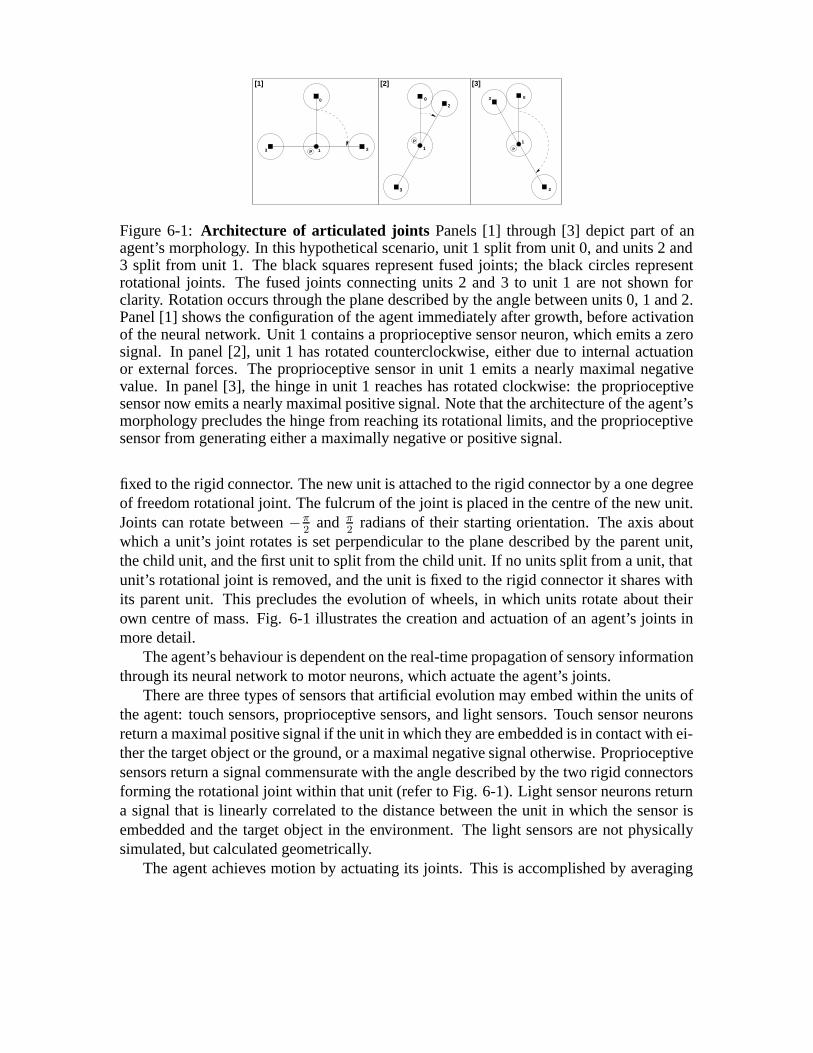
P

2

PP

0

1 23

0

1

2

3

03

1

[2][1] [3]

Figure 6-1: Architecture of articulated joints Panels [1] through [3] depict part of anagent’s morphology. In this hypothetical scenario, unit 1 split from unit 0, and units 2 and3 split from unit 1. The black squares represent fused joints; the black circles representrotational joints. The fused joints connecting units 2 and 3 to unit 1 are not shown forclarity. Rotation occurs through the plane described by the angle between units 0, 1 and 2.Panel [1] shows the configuration of the agent immediately after growth, before activationof the neural network. Unit 1 contains a proprioceptive sensor neuron, which emits a zerosignal. In panel [2], unit 1 has rotated counterclockwise, either due to internal actuationor external forces. The proprioceptive sensor in unit 1 emits a nearly maximal negativevalue. In panel [3], the hinge in unit 1 reaches has rotated clockwise: the proprioceptivesensor now emits a nearly maximal positive signal. Note that the architecture of the agent’smorphology precludes the hinge from reaching its rotational limits, and the proprioceptivesensor from generating either a maximally negative or positive signal.

fixed to the rigid connector. The new unit is attached to the rigid connector by a one degreeof freedom rotational joint. The fulcrum of the joint is placed in the centre of the new unit.Joints can rotate between−π

2and π

2radians of their starting orientation. The axis about

which a unit’s joint rotates is set perpendicular to the plane described by the parent unit,the child unit, and the first unit to split from the child unit. If no units split from a unit, thatunit’s rotational joint is removed, and the unit is fixed to the rigid connector it shares withits parent unit. This precludes the evolution of wheels, in which units rotate about theirown centre of mass. Fig. 6-1 illustrates the creation and actuation of an agent’s joints inmore detail.

The agent’s behaviour is dependent on the real-time propagation of sensory informationthrough its neural network to motor neurons, which actuate the agent’s joints.

There are three types of sensors that artificial evolution may embed within the units ofthe agent: touch sensors, proprioceptive sensors, and light sensors. Touch sensor neuronsreturn a maximal positive signal if the unit in which they are embedded is in contact with ei-ther the target object or the ground, or a maximal negative signal otherwise. Proprioceptivesensors return a signal commensurate with the angle described by the two rigid connectorsforming the rotational joint within that unit (refer to Fig. 6-1). Light sensor neurons returna signal that is linearly correlated to the distance between the unit in which the sensor isembedded and the target object in the environment. The light sensors are not physicallysimulated, but calculated geometrically.

The agent achieves motion by actuating its joints. This is accomplished by averaging

the activations of all the motor neurons within each unit, and scaling the value between−π

2and π

2. Torque is then applied to the rotational joints such that the angle between the

two rigid connectors forming the joint matches this value. The desired angle may not beachieved if: there is an external obstruction; the units attached to the rigid connectors ex-perience opposing internal or external forces; or the values emitted by the motor neuronschange over time. Note that failure to achieve the desired angle may be exploited by evo-lution, and may be a necessary dynamic of the agent’s actions. If a unit contains no motorneurons, the rotational joint in that unit is passive.

Internal neurons can also be incorporated by evolution into an agent’s neural network,in order to propagate signals from sensor to motor neurons. Two additional neuron typesare available to evolution. Bias neurons emit a constant, maximum positive value. Oscil-latory neurons emit a sinusoidal output signal. The summed input to an oscillatory neuronmodulates the frequency of the output signal, with large input signals producing an out-put signal with a high frequency, and low input signals producing a low frequency outputsignal.

6.2.2 Differential Gene Expression

Unlike the recursive parametric encoding schemes mentioned above, each genome in theAO system is treated as a genetic regulatory network ([Kauffman, 1993, Jakobi, 1995,Eggenberger, 1997, Reil, 1999]), in which genes produce gene products that either havea direct phenotypic effect or regulate the expression of other genes.

For each genome to be evaluated in the population, it is first copied into the single unitfrom which the eventual fully-formed agent develops. The genome is then scanned by aparser, which marks the site of promotor sites. Promotor sites indicate the starting positionof a gene along the genome. A value in the genome is treated as a promotor site if the valueis below n

l, wheren is the average number of genes that should appear within each initial

random genome, andl is the length of genomes in the initial, random genetic algorithmpopulation. This is done so that, given a starting population of random genomes, eachgenome will contain, on average, the desired number of genes. In the results reported inthe next section,l = 100 andn = 10, causing values between0.00 and0.10 to serve aspromotor site indicators.

Fig. 6-2 provides a pictorial representation of a genome directing the growth of anagent. The seven floating-point values following a gene’s promotor site supply the parame-ter values for the gene. If the first value (P1 in Fig. 6-2) is less than0.5, gene expression isrepressed by presence of the gene product which regulates its expression; otherwise geneexpression is enhanced by presence of its regulating gene product. The second value (P2in Fig. 6-2) indicates which of the24 possible gene products regulates the gene’s expres-sion. The third value (P3 in Fig. 6-2) indicates which of the24 possible gene products isproduced if this gene is expressed. The fourth value (P4 in Fig. 6-2) indicates which of the6 gene product diffusion sites the gene product is diffused from if this gene is expressed.The fifth value (P5 in Fig. 6-2) indicates the concentration of the gene product that should

G1 G2 G 3 G 4 G n

0.500.03 (1) (22) (3) (1) 0.37 0.0P1

P1

P2

P2

P3

P3

P4

P4

P5

P5

P6

P7

P7

P6

C 2

C 3

C 1

C 4

C 2

C 3

C 1

C 4

TSTS

M M

. . .

Pr

Pr

0.08 (0) (3) (22) 0.91 0.50 0.99(4)

1.0 1.0

Figure 6-2: Ontogenetic interactions in a developing agentTwo structural units of anagent are shown above, but only displayed in two dimensions for clarity. For this reason,only four of the six gene product diffusion sites are shown; the other two lie at the top andbottom of the spherical units. The genome of the agent is displayed, along with parametervalues for two genes. The values in parentheses indicate that these values are rounded tointeger values. GeneG1 indicates that it is repressed (parameterP1) by concentrations ofgene product3 (P2) between0.5 and0.99 (P6, P7). Otherwise, it diffuses gene product22 (P3) from gene product diffusion location4 (P4), indicated in the diagram byC4. Notethat genesG1 andG3 emit gene products which regulate the other’s expression. The thickdotted lines indicate gene product diffusion between diffusion sites within a unit; the thindotted lines indicate gene product diffusion between units. Both units contain a touchsensor neuron (TS) and a motor neuron (M) connected by excitatory synapses.

be injected into the diffusion site if the gene is expressed. The sixth and seventh values (P6andP7 in Fig. 6-2) denote the concentration range of the regulating gene product to whichthe gene responds. If the concentration of the regulating gene product to which the generesponds is within this range, and the gene is enhanced by presence of its regulating geneproduct, the gene is expressed; otherwise, gene expression is repressed. Genes that are re-pressed by their regulating gene product are expressed if the gene product’s concentrationis outside the denoted range, and repressed otherwise.

After the genes in the genome have been located, the originating unit of the agent to begrown is injected with a small amount of gene product at diffusion site1. Due to gene prod-uct diffusion, a gradient is rapidly established in this first unit, among the6 diffusion sites.This is analogous to the establishment of a gradient of maternal gene product in fruit flies,which leads to the determination of the primary body axis [Anderson and Nüsslein-Volhard, 1984],and breaking of symmetry in early embryogenesis. It can be seen from Fig. 6-3 that thedegree of symmetry in evolved agents varies, and is under evolutionary control.

As the injected gene product diffuses throughout the unit, it may enhance or repressthe expression of genes along the genome, which in turn may diffuse other gene products.There are24 different types of gene products. Two affect the growth of the unit in whichthey diffuse. At each time step of the development phase, the difference between the con-

centration of these two chemicals is computed. If the difference is positive, the radius ofthe unit is increased a small increment; if the difference is negative, the unit does not growin size. Thus these two chemicals function as growth enhancer and growth repressor, re-spectively. If the radius of a unit reaches twice that of its original radius, a split event isinitiated. The radius of the parent unit is halved, the gene product diffusion site with themaximum concentration of growth enhancer is located, and a new unit is attached to theparent unit at this position. Half of the amounts of all gene products at this diffusion siteare moved to the neighbouring diffusion site in the new unit. A copy of the genome is as-signed to the new unit. The gene expression patterns of the parent and child units are nowindependent, except for indirect influence through inter-unit diffusion of gene products.

There are then17 other chemicals which affect the growth of the agent’s neural network,and are explained in the next section. Finally, five gene products have no direct phenotypiceffect, but rather may only affect the expression of other genes. That is, concentrations ofthese gene products at diffusion sites can enhance or repress gene expression in that unit(like the other19 gene products), but cannot modify neural structure, or stimulate or repressthe growth of that unit.

All 24 gene products share the same fixed, constant diffusion coefficients. For each timestep that a gene emits gene product, the concentration of that gene product, at the diffusionsite encoded in the gene, is increased by the amount encoded in the gene (which rangesbetween0.0 and1.0), divided by100. All gene product concentrations, at all diffusion sites,decay by0.005 at each time step. Gene products diffuse between neighbouring diffusionsites within a unit at one-half this rate. Gene products diffuse between neighbouring unitsat one-eighth the rate of intra-unit diffusion.

6.2.3 Neural Growth

Cellular encoding [Gruau and Quatramaran, 1996] has been incorporated into our model toachieve the correlated growth of morphology and neural structure in a developing agent.Cellular encoding is a developmental method for evolving both the architecture and synap-tic weights of a neural network. The process involves starting with a simple neural networkof only one or a few neurons, and iteratively or recursively applying rewrite rules thatmodify the architecture or synaptic weights of the growing network.

In our model, for each new unit that is created, including the first unit, a small neuralnetwork is created as follows: A touch sensor neuron (TS) is placed at diffusion site1,a motor neuron (M) is placed at diffusion site2, and a synapse with a weight of1.0 isconnected from the sensor neuron to the motor neuron (refer to Fig. 6-2). When a unitundergoes a split event, any neurons at the diffusion site where the split event was initi-ated are moved to the neighbouring diffusion site of the new unit. For example, if a unitsplits, and the new unit is attached near its northern face, all the neurons in the northerndiffusion site of the parent unit are moved to the southern diffusion site in the new unit.Neurons may also move from one diffusion site to another within a unit, depending on theconcentrations of gene products at those sites. The combination of these dynamics may

lead to the directed migration of neurons across the units as they divide. As they migrate,synapses connecting these neurons are maintained: although this process is different fromthe neural growth cone model (in which biological neurons innervate distant cells using ex-ploratory synaptic outgrowths [Kater and Guthrie, 1990]) and instantiations of this model[Delleart and Beer, 1994, Jakobi, 1995], it does allow for neurons in distant units to remainconnected.

Each of the17 gene products responsible for neural development correspond to onerewrite operation that modifies local neural structure. At each diffusion site, two pointersare maintained: the first pointer indicates which synapse will undergo any synaptic modi-fication operations; the second pointer indicates which neuron will undergo any neuronalmodification operations. The17 rewrite rules correspond to serial and parallel duplicationof neurons; deletion of neurons and synapses; increase and decrease of synaptic weight;duplication of synapses; neuron migration within a unit; changing of the afferent and effer-ent target of synapses; and changing of neuron type. If the concentration of one of these17gene products at a diffusion site exceeds0.8, and there is neural structure at that site, thecorresponding operation is applied to the neural structure there. Once development is com-plete, the neural network that has grown within the agent is activated. At each time step ofthe evaluation period, the input to each neuron is summed, and thresholded using the acti-vation function 2

1+e−s −1, wherex is the neuron’s summed input. Neuron values can rangebetween1 and−1. Using this neural development scheme, the AO system is able to evolvedynamic, recurrent neural networks that propagate neural signals from sensor neurons tomotor neurons distributed throughout an agent’s body.

6.3 Results and Analysis

The evolutionary runs reported in this section were conducted using a variable length ge-netic algorithm; the genomes were strings of floating-point values ranging between0.00and1.00, rounded to a precision of two decimal places. A population size of200 was used,and each run lasted for200 generations. All genomes in the initial random population havea starting length of100 values. The mutation rate was set to produce, on average, randomreplacement of a single value for each new genome. Unequal crossover was employed,which allowed for gene duplication and deletion. Tournament selection, with a tournamentsize of2, was used to select genomes to participate in crossover.

As in [Bongard and Pfeifer, 2003], agents are evaluated in a physically-realistic vir-tual environment using a commercially available physics-based simulation package4. Eachgenome in the population is evaluated as follows: The genome is copied into a single unit,which is then placed in a virtual, three-dimensional environment. A target cube is placed20 units5 to the north of the unit; the sides of the cube are70 units long. Morphological

4MathEngine PLC, Oxford, UK,www.mathengine.com5Spatial distance in the physics-based simulator is relative; we treat a ‘unit’ as equal to the default radius

of a newly-created unit.

a) b)

c) d)

Figure 6-3:Four agent morphologiesThe block is not shown in the figure for the sake ofclarity, but lies just to the left of the agents. The rigid connectors are also not shown. Thewhite units indicate the presence of both sensor and motor neurons within that unit. Thelight gray units indicate the presence of both sensor and motor neurons in that unit, but theone or more motor neurons do not actuate the rotational joint in that unit either becausethere are no input connections to the motor neuron, or because there is no joint within thisunit. The dark gray units indicate the presence of sensor neurons, but no motor neurons.The black units indicate the unit contains neither sensor nor motor neurons.

and neural development is allowed to proceed, as described in the previous section, for500time steps. After the development phase, the neural network is activated, and the agent isallowed to operate in its virtual environment for1000 time steps. The fitness of an agentis given as

∑1000i=2 n(t(i− 1))− n(t(i)), wheren(t(i)) is the northern distance of the centre

of the cube from the origin at timet. Thus the agent is rewarded for reaching the cube asfast as possible, and pushing it as far as possible. By making the cube much larger thanthe units comprising an agent, we can exert indirect selection towards large agents: agentsmust have a large mass in order to exert a large force against the cube. Agents a) and b) inFig. 6-3 depict the morphologies of the most fit agents from two independent runs. Agentsc) and d) were the most fit agents at generation110 and130 of the run shown in Fig. 6-4.

In order to detect the presence of hierarchical, repeated structure in evolved agents, thelocal neural structure within units was used as a signature to distinguish between units. Forinstance in agent a) in Fig. 6-3, the two neighbouring units that have lost their motor andsensory capabilities are repeated twice. In the right-hand agent, the three most distal unitsin the three main appendages have also lost their motor and sensory capabilities.

The most fit agent from each of the nine evolutionary runs was extracted, and the num-ber of motor and sensor neurons in each unit of each appendage was counted. The talliesfor each unit are reported in Fig. 6-5. Because the units comprising an agent are organizedas directed trees, appendages can be determined as follows: for each terminal unit in theagent, traverse up the tree until a unit is found with more than one child unit. The units thatwere traversed, minus the last one counted, comprise an appendage.

Figure 6-4:Results from a typical run. Genome length was found to be roughly propor-tional to the number of genes, and is not plotted.

Figure 6-5:Neural composition of nine evolved agentsEach symbol indicates the numberof motor and sensor neurons in a structural unit. Neural structure is only reported for unitsthat are part of an appendage. Units comprising an appendage are linked by gray lines.Gray symbols indicate no rewrite rules have been applied to the neural structure in that unit;black symbols indicate units in which genetic manipulation of local structure has occurred.The gene expression patterns of the four units indicated by bold symbols is shown in Fig.6-6. Agent1 corresponds to agent b) in Fig. 6-3.

Finally, the gene expression patterns of four units are reported in Fig. 6-6. Units a) andc) give rise to appendages with similar patterns of local neural structure, and themselveshave similar internal neural structure. Units b) and d) do not give rise to further structure,and have similar neural structure. This structure is different from units a) and c). The four

a)

b)

c)

d)

Figure 6-6: Gene expression patterns for four units. Dark gray and light gray bandscorrespond to periods of gene activity and inactivity, respectively. Four genes are markedby asterisks; the expression pattern of these genes is similar in units a) and c), but differentin units b) and d). The expression times of these genes are darkened for clarity. Genesthat are always on or always off during ontogeny are not shown. Note the evolved genefamilies, which have similar expression patterns.

units are indicated in bold in Fig. 6-5. Units a) through d) all split from the same parentunit during ontogeny, but appear at increasingly later times during the agent’s development.

6.4 Discussion and Future Work

Fig. 6-4 indicates that no agent is able to push the block until generation 20; this eventis accompanied by a doubling in the number of genes carried by these more fit agents.However, the gene complement of agents does not increase considerably during the rapidfitness increase which occurs around generation120. Agents c) and d) in Fig. 6-3 indicatethat this fitness increase was accomplished by a radical increase and reorganization of theagent’s morphology and neural control. This suggests that the AO system is exhibitingthat predicted property of indirect encoding schemes, that is, large increases in phenotypic

complexity6 without corresponding large increases in genome size7.Fig. 6-5 indicates that invariably, evolution converges on agents that exhibit hierarchical

repeated structure. This can be seen most clearly in the first agent in Fig. 6-5, in whichthe first agent contains three similar appendages with three distal units each containingneither motor nor sensor neurons. Moreover, Fig. 6-5 indicates that genetic changes tolocal neural structure can be repeated both within an appendage—as seen by the deletionof function in the three distal units—and across appendages—as seen by the triple deletionof function repeated in three different appendages.8 In other words, agents tend to haveappendages in which local neural structure is repeated along the length of the appendage,and appendages themselves are repeated. It is important to note that this structure—whichwe, as observers, consider hierarchical, repeated structure—is the result of the complex,dynamical interplay between the evolved genetic regulatory networks, the developmentalprocess, and the selection pressure exerted on the evolving population. This suggests thatthe study of genetic regulatory networks should not be conducted in isolation, but ratherin the context of embodied agents evolved for a specific task. This would then give us aclearer picture of how both natural and artificial evolution shape such regulatory networksover time.

Finally, Fig. 6-6 indicates that the units that give rise to similar appendages have similargene expression patterns, even though they appear at different times during ontogeny. Sim-ilarly, the gene expression patterns of two other units, which appear at roughly the sametime as the other two units, correspond. However, the gene expression patterns are differ-ent between these two pairs of units. This is shown by the expression of the first markedgene in units a) and c), but not in b) and d); a short expression band for the other threemarked genes appears during late ontogeny in units b) and d), but not in a) and c). Thisindicates that, even though all four of these units originated from the same parent unit, andat roughly the same time during ontogeny, the units which gave rise to appendages have ashared pattern of expression that differs from the pair that does not give rise to appendages.This result suggests that future studies might uncover one or a small set of genes that leadto the growth of higher-order structure when active, but repress such growth when inactive.These genes would serve as analogues ofHox genes in biological organisms, and wouldindicate that such genes are the natural result of evolution when coupled with ontogeny anddifferential gene expression. Our future studies will also include more detailed analysis ofthe evolved genetic networks.

6In this context, complexity is simply taken as the number and organization of units, and variation in localneural structure within those units.

7As mentioned earlier, I view phenotypic complexity as the numbers and types of basic units comprisingthe agent. Genotypic complexity is viewed as the number of genes contained in the genome, as increasednumbers of genes usually corresponds to increased numbers and types (ie., which chemical they emit) ofgenes. Both this phenotypic and genotypic view of complexity is informal, but is sufficient to demonstratethat one (phenotypic complexity) can increase without required that the other (genotypic complexity) does aswell.

8From visual inspection of these agent’s behaviours, it seems as if these appendages use a whiplike mo-tion, requiring strong actuation at the proximal end and little or no actuation at the distal end.

6.5 Conclusions

To conclude, this paper has demonstrated that a minimal model of biological development,coupled with a genetic algorithm that allows for gene duplication and deletion, is sufficientto evolve agents that perform a non-trivial task in a physics-based virtual environment.Moreover, this system—referred to as artificial ontogeny—is sufficient to produce hierar-chical, repeated phenotypic structure. In addition, it has been shown that the inclusion ofdifferential gene expression in artificial ontogeny dissociates the information content of thegenome from the complexity of the evolved phenotype.

Both of these properties point to the high evolvability of the AO system: both theproduction of hierarchical, repeated organization and the dissociation of genotypic andphenotypic complexity are desirable if artificial evolution is to prove useful for the designof robots that solve increasingly complex tasks, the ultimate goal of evolutionary roboticsresearch.

Chapter 7

Evolving Modular Genetic Regulatory Networks1

Abstract

In this paper we introduce a system that combines ontogenetic development and artificialevolution to automatically design robots in a physics-based, virtual environment. Throughlesion experiments on the evolved agents, we demonstrate that the evolved genetic regu-latory networks from successful evolutionary runs are more modular than those obtainedfrom unsuccessful runs.

7.1 Literature Review

The recent renaissance of ’evo-devo’[White, 2001]—evolutionary developmental biology—is causing a radical change in our understanding of how selection pressure shapes the or-ganism’s underlying genetic regulatory network (GRN).

Several startling discoveries have been made regarding the so-called Hox genes (mas-ter control genes that specify and order the body segments in most metazoan species[Gehring and Ruddle, 1998]), including mounting evidence that these genes are highlyconserved over many species[Cohen, 1993, Schierwater and Desalle, 2001], diversificationof Hox gene clusters has led to a diversification in animal body plans [Finnerty, 2000,Meyer, 1998], and that these genes are arranged along the chromosome in the same orderthat they are expressed along the anterior-posterior axis of the embryo[Lewis, 1992]. How-ever, insights into how selection pressure has shaped the evolution and diversification ofsuch genes is only now beginning to appear in the literature [Carroll, 2000, Mann, 1997].

In parallel to this, both neuroscience researchers and evolutionary biologists have postu-lated that modularity (integration of functionally related structures, and dissociation of un-related structures) is necessary at both phenotypic [Tononi et al., 1994, Tononi et al., 1999]

1Appeared as Bongard, J. C., “Evolving Modular Genetic Regulatory Networks”, inProceedings of theIEEE 2002 Congress on Evolutionary Computation (CEC2002), IEEE Press, pp. 1872–1877, 2002

82

Figure 7-1:a-e: Images taken fromt0, t75, t150, t225 andt300 during the growth phase ofan evolved agent. The units are darkened in proportion to how many neurons and synapsesthey contain.f: t0 of the evaluation phase. The grey units contain motorized joints.

and genotypic [Wagner and Altenberg, 1996, Wagner, 1996] levels in order to evolve com-plex structures.

In the field of evolutionary robotics, evolutionary computation is now being used toevolve both the brains and bodies of virtual [Sims, 1994, Adamatzky et al., 2000] and real-world robots [Lipson and Pollack, 2000], and focus is increasingly coming to bear on mak-ing the genetic encoding of these systems as modular and compact as possible in order to in-crease evolvability [Gruau, 1994, Calabretta et al., 2000]. Eggenberger [Eggenberger, 1997]first incorporated GRNs into an evolutionary simulation to evolve three-dimensional shapes.In this paper I report new results obtained from the Artificial Ontogeny system (AO),which grows virtual agents from GRNs and evaluates them in a physically-realistic, three-dimensional virtual environment [Bongard and Pfeifer, 2003].

7.2 Methods

Artificial Ontogeny extends the genetic algorithm to include ontogenetic development. Inthe results presented below, agents are tested for how fast they can travel over an infinitehorizontal plane during a pre-specified time interval. The fitness determination is a two-stage process: the agent is first grown from a GRN (the growth phase), and then evaluatedin its virtual environment (the evaluation phase) (Fig. 7-1).

Agents are composed of one or more cylindrical morphological units and zero or more

Figure 7-2: a: A hypothetical agent at the beginning of growth. The anterior direction(the direction the agent must move in order to gain fitness) is indicated (ANT), as is theposterior direction (POS). A genome, a motor neuron (M) and two maternal TFs (M1, M2)are injected into the single, beginning morphological unit (U1). The unit contains six TFdiffusion sites (1-6). The genome contains five genes:G1, G3, G4 are structural genes;G2 andG5 (outlined in bold) are regulatory genes.G3 andG5 are initially switched on,and begin to diffuse TFs into the unit; the other genes are initially switched off (light greyindicates expression; dark grey indicates repression).b: After several time steps,U1 hassplit twice, producing neighbouring daughter unitsU2 andU3, which are attached to it byone degree-of-freedom damped, torsional joints. The genome has been copied intoU2 andU3, where different combinations of TF concentrations have changed the states of someof the genes.U1 has been lengthened by TF2, which increases unit length, released byG3 at diffusion site 5.M1 andM2 have diffused throughout the unit. The motor neuronin U1 has differentiated into a local neural circuit through combined gene action (T=touchsensor,CPG=central pattern generator,N=neuron).c: The fully grown agent from whichall genetic material has been removed, in preparation for agent evaluation. The joint nearU2 is active, because it receives motor commands from the neural circuit inU2. The jointnearU3 is passive, and will swing freely during the evaluation phase because the motorneuron inU3 has been deleted.

sensors, motors, neurons and synapses. At the beginning of the growth phase, the genometo be tested and a motor neuron are inserted into a single unit. Two different transcrip-

tion factors (TFs) are injected into the anterior and posterior poles of the unit, in orderto allow the GRN to establish major body axes in the developing agent, if required (thishas been shown to be one of the primary roles of maternal TF diffusion during earlydevelopment[Anderson and Nüsslein-Volhard, 1984]). The maternal TFs affect the expres-sion of the zero or more genes lying along the genome embedded in the starting unit, whichin turn may begin to emit TFs throughout the unit. The TFs may directly affect the pheno-type of the developing agent: there are 23 pre-defined phenotypic transformations that TFscan initiate, such as increasing the length of a unit, causing a unit to split into two units, oradding, deleting or modifying the properties of the agent’s neurons or synapses (Fig. 7-2).

Unlike the recursive parametric encoding schemes mentioned above, each genome inthe AO system is treated as a genetic regulatory network [Kauffman, 1993, Eggenberger, 1997,Reil, 1999], in which genes produce transcription factors that either have a direct pheno-typic effect or regulate the expression of other genes.

Each genome to be evaluated is scanned by a parser, which marks the site of promotorsites. Promotor sites indicate the starting position of a gene along the genome, and arenot hand-coded, but rather the number and position of them is under evolutionary control,similar to the method employed in [Reil, 1999]. On average, there are10 promotor sites,and thus 10 genes, found in any randomly generated genome.

Fig. 7-3 shows a magnification of geneG3 from Fig. 7-2. The six floating-point valuesfollowing a gene’s promotor site supply the parameter values for the gene. The first value(P1) indicates which of the20 possible TFs regulates the gene’s expression. The secondvalue (P2) indicates which of the23 possible TFs is produced if this gene is expressed. Thethird value (P3) indicates which of the6 TF diffusion sites the TF is diffused from if thisgene is expressed. The fourth value (P4) indicates the concentration of the TF that shouldbe injected into the diffusion site if the gene is expressed. The fifth and sixth values (P5andP6) denote the concentration range of the regulating TF to which the gene responds.

All 43 TFs (23 TFs that directly affect the phenotype, and 20 regulatory TFs) sharethe same fixed, constant diffusion coefficients. For each time step that a gene emits itsTF, the concentration of that TF, at the diffusion site encoded in the gene, is increasedby the amount encoded in the gene (which ranges between0.0 and1.0), divided by100.All TF concentrations, at all diffusion sites, decay by0.005 at each time step. TFs diffusebetween neighbouring diffusion sites within a unit at one-half this rate. TFs diffuse betweenneighbouring units at one-eighth the rate of intra-unit diffusion.


There are two types of sensors that artificial evolution may embed within the units of theagent: touch sensors and proprioceptive sensors. Touch sensor neurons return a maximalpositive signal if the unit in which they are embedded is in contact with either the targetobject or the ground, or a maximal negative signal otherwise. Proprioceptive sensors returna signal commensurate with the angle described by the two rigid connectors forming therotational joint within that unit. The agent can also contain central pattern generator (CPG)neurons. These neurons emit a sinusoidal output signal: their frequency is modulated by the

Figure 7-3:A sample gene.This gene (G3 in Fig. 7-2) emits TF 2 from diffusion site 5(DS5) if it is expressed (the concentration of TF 2 is increased by 0.03 atDS5during eachtime step of the growth phase thatG3 is expressed). If the average concentration of TF 37in the current unit is between 0.23 and 0.93 the gene is expressed; otherwise, it is repressed.The gene is flanked by non-coding values (Nc).

strength of the incoming signal (large positive input produces a high frequency, and largenegative input produces a low frequency), and their phase is set relative to the time step(during the growth phase) when they are formed. Internal neurons can also be incorporatedby evolution into an agent’s neural network, in order to propagate signals from sensor tomotor neurons. Finally, bias neurons emit a constant, maximum positive value.

The agent achieves motion by actuating its joints. This is accomplished by averagingthe activations of all the motor neurons within each unit, and scaling the value between− π

2

and π2

(these minimum and maximum joint angles may be reduced by the presence of oneof the TFs that affects morphogenesis). Torque is then applied to the rotational joints suchthat the angle between the two rigid connectors forming the joint matches this value. Thedesired angle may not be achieved if: there is an external obstruction; the units attached tothe rigid connectors experience opposing internal or external forces; or the values emittedby the motor neurons change over time. Note that failure to achieve the desired angle maybe exploited by evolution, and may be a necessary dynamic of the agent’s actions. If a unitcontains no motor neurons, the rotational joint in that unit is passive.

7.3 Results

The agents reported in this section were evaluated in a three-dimensional, physically-realistic simulation package2. During each time step of the evaluation, sensor readings aretaken, the neural network is updated, and the motor commands are translated into torques.The torques are passed to the simulator, which updates the positions, velocities and orien-tations of each of the agent’s units. The updates are also affected by simulated externalforces such as gravity, inertia, friction and collision or contact with the ground plane3.

Sixty independent evolutionary runs of 300 generations each were conducted, using a

2Critical Mass Labs,www.cm-labs.com.3By evaluating the agent in a physically realistic simulation, agents can evolve to take advantage of their

environment, such as using gravity and momentum to move non-actuated joints in a useful manner. Also, itmay be easier to translate evolved solutions into real-world robots.

population size of 300. The initial population was composed of 300 strings of 200 floating-point values, rounded to two decimal places and ranging between0.00 and1.00. Genomeswere evolved to maximize the fitness function

f = s + (pz(t500)− pz(t250))500∑t=1

utot∑i=1

|ji(t)|, (7.1)

s = n + m + sy + synz + onz, (7.2)

n =

{utot : utot ≤ 3

3 : utot > 3(7.3)

m =

{1 : stot > 0 and mtot > 00 : otherwise

(7.4)

whereutot is the number of units comprising the agent;ji(t) is the desired angle com-mand sent to jointj in unit i at time stept; andpz(t500) andpz(t250) are the z-componentsof the anterior-most unit’s position at the end of, and halfway through the evaluation pe-riod, respectively4. s is a shaping function: it awards agents that have not yet achieved anylocomotion for particular phenotypes that favour the discovery of locomotion.n awards foragents that are composed of at least three units, andm awards for creatures that contain atleast one sensor and one motor (stot andmtot denote the total number of sensors and motorneurons in the agent, respectively).sy = 1, synz = 1 andonz = 1 if the agent contains atleast one synapse, one synapse with non-zero weight, or one non-zero motor neuron output,respectively, and are set to zero otherwise. The shaping function allows evolution to rapidlyproduce an agent that exhibits some active behaviour. An alternative approach would havebeen to seed evolution with minimally behaving agents, and omit the shaping function.

Strong elitism was employed; the best150 genomes at each generation were retained.The mutation rate was set to produce, on average, random replacement of a single valuefor each new genome. Also, new genomes had a10% chance of having a substring of theirvalues excised (the length of the excised substring was chosen between 1 andl − 1 with auniform distribution, wherel is the length of the genome), and a10% chance of two non-overlapping substrings (chosen between 1 andl

2− 1 with uniform distribution) from being

swapped within the genome. Unequal crossover was employed, which allowed for geneduplication and deletion. Tournament selection, with a tournament size of3, was used toselect genomes to participate in crossover.

Fig. 7-1f shows the morphology of the most fit agent taken from one of the evolutionaryruns; Figs. 7-4 and 7-7b show the morphologies of the most fit agents from two other runs.

In several of the runs, forward locomotion did not evolve; agents either exhibited ran-dom actuation, or discovered a way to fall over just aftert250. In other runs, small agentscomposed of no more than6 units, and only1 or 2 active joints, discovered forward loco-motion. However in two runs, large agents (Figs. 7-1f and 7-4) with several actuated joints

4By ignoring any locomotion beforet250, agents that passively fall over receive low fitness values.

Figure 7-4: The morphology of the most successful agent from one evolutionary run (wild-type).

achieved forward locomotion. The GRN of one of these agents is shown in Fig. 7-5. Thisgenome contained66 active genes—genes that were expressed for at least one time step, inat least one of the agent’s units. Regulatory genes are depicted as boxes with bold edges;the other genes are structural genes. The black genes indicate the regulatory genes target-ted for the lesion experiments shown in Fig. 7-6. The dark grey structural genes denotethose genes that participate in neurogenesis: they guide the growth of the agent’s neuralstructure. The grey structural genes participate in morphogenesis: they direct the growthof the agent’s body. The numbers inside the gene indicate which TF is emitted by thatgene. The numbers outside the genes indicate their relative position along the gene: gene1 is the first active gene in the genome; gene 2 is the second, and so on. Arrows indicategene regulation: for example, genes 45 and 46 are regulated by regulatory TF 13, whichis emitted by genes 49 and 59. Genes 7, 11 and 62 are regulated directly by the anteriormaternal TF. Genes 13 and 23 have evolved to emit the posterior maternal TF.

The set of genes that directly regulate the most neurogenesis genes (for this agent, genes10, 34, 35, 60 and 63) were selected for mutation. The agent was regrown with these genessuppressed in all units: Fig. 7-6a shows the morphology of this loss-of-function mutant.The agent was then regrown again, with these genes expressed in all units: Fig. 7-6b showsthe morphology of this gain-of-function mutant. The expression pattern differences of the66 active genes between the first unit of the original (wild-type) agent5 and the loss-of-

5The term ‘wild-type’ refers to the fact that the agent was grown from a genome taken directly from acompleted evolutionary run, and no additional modifications have yet been made to it.

Figure 7-5: The underlying GRN specifying the growth of the agent shown in Figure 7-4.

function mutant are shown in Fig. 7-6c. The expression pattern differences of the 66 activegenes between the first unit of the original agent and the gain-of-function mutant are shownin Fig. 7-6d.

7.4 Analysis

As can be seen from Figs. 7-6c and 7-6d, the supression or enhancement of the five tar-getted regulatory genes has a larger effect on the structural neurogenesis genes than thaton the morphogenesis genes. Similarly, the morphologies of the loss-of-function and gain-of-function mutants (Figs. 7-6a and 7-6b) are quite similar to that of the wild-type agent.However, in both agents, the neural disruption was severe enough such that none of thejoints were actuated. This indicates that there is high pleitropy (co-regulation) between theneurogenesis genes, and lower pleitropy between neurogenesis and morphogenesis genes.In other words, a dissociation between regulation of neurogenesis and morphogenesis hasoccurred: that is, evolution can experiment with different body plans and not disrupt neu-rogenesis, and can experiment with different neural components on the same body plan.

Figure 7-6:Results from a lesion experiment. a, The agent regrown with regulatory genes10, 34, 35, 60 and 63 repressed in all units (loss-of-function).b, The agent regrown with thetargetted genes expressed in all units (gain-of-function).c, Differences in gene expressionbetween the first units of the wild-type and loss-of-function agents. Black bars indicatethe targetted regulatory genes; dark grey bars indicate structural genes that influence neuralgrowth; grey bars indicate structural genes that influence morphological growth; light greybars indicate other regulatory genes.d, Differences in gene expression between the firstunits of the wild-type and gain-of-function agents.

A measure has been formulated to quantify this genetic modularity, using the weightedsums

NLW =

∑utotu=1 t(u) ∑300

t=1

∑gni=1 |gW

i (t)− gLi (t)|∑utot

u=1 t(u)(7.5)

MLW =

∑utotu=1 t(u) ∑300

t=1

∑gmi=1 |gW

i (t)− gLi (t)|∑utot

u=1 t(u)(7.6)

NGW =

∑utotu=1 t(u) ∑300

t=1

∑gni=1 |gW

i (t)− gGi (t)|∑utot

u=1 t(u)(7.7)

MGW =

∑utotu=1 t(u) ∑300

t=1

∑gm

i=1 |gWi (t)− gG

i (t)|∑utotu=1 t(u)

(7.8)

whereNLW andNG

W indicate the expression differences between the neurogenesis genesin the wild-type agent and loss-of-function mutant, and the wild-type agent and gain-of-function mutant, respectively. A value of zero indicates there were no expression differ-ences between any of the neurogenesis genes; a value of one indicates that whenever aneurogenesis gene—at any time step in any unit of the wild-type agent—is expressed (orsuppressed), it is suppressed (or expressed) during that time step, in that unit, of the mu-tant. Similarly,ML

W andMGW indicate the expression differences between the morphogen-

esis genes in the wild-type agent and loss-of-function mutant, and the wild-type agent andgain-of-function mutant, respectively.utot here indicates the total number of units compris-ing the wild-type, loss-of-function or gain-of-function agent with the minimum number ofunits. gn andgm indicate the number of active neurogenesis and morphogenesis genes inthe wild-type agent, respectively.gW

i (t) > 0, gLi (t) > 0 andgG

i (t) > 0 if genei in thewild-type, loss-of-function or gain-of-function agent is expressed at time stept; and are setto zero otherwise.t(u) indicates the number of time steps for which unitu is present duringthe growth phase:t(1) = 300, and units appearing later during the growth phase have lowervalues.

In some agents, suppressing or enhancing the targetted regulatory genes disrupts themorphology such that the second and subsequent units in the loss-of-function or gain-of-function mutants appear earlier or later than they do in the wild-type agent. Thus, in orderto compare the expression patterns of genes between these units, the expression patterns areexpanded from binary strings with lengths less than300 to floating-point strings of length300 with values in[0, 1] using bilinear scaling[Cox and Cox, 2000].

Now, the pairs[NLW , ML

W ] and [NGW , MG

W ] indicate the relative neurological and mor-phological effects caused by artificially suppressing or enhancing the expression of target-ted regulatory genes. This measure was applied to the most fit agent from each of the 60runs; the targetted gene set was chosen by selecting those regulatory genes that directlyco-regulated the maximum number of neurogenesis genes. In some agents, the loss-of-function mutation had a greater effect than the gain-of-function mutation, and in otheragents, the reverse case was true, depending on how the targetted genes are expressed inthe wild-type agent. In order to compare mutational effect, ifNL

W > NGW in an agent, then

[NLW , ML

W ] was retained and[NGW , MG

W ] was discarded; otherwise,[NGW , MG

W ] was retainedand[NL

W , MLW ] was discarded. Fig. 7-7a plots these 60 remaining value pairs: it shows the

relative neurological versus morphological effects of the lesion experiment on each agent.As can be seen, the two runs that produced the large, locomoting agents produced more

highly modular GRNs than the GRNs evolved in the other evolutionary runs: lesioning ofthe targetted genes in these agents had quite a drastic neurological effect, but a relativelymild morphological effect. Moreover, the agent with the most modular GRN had the max-

Figure 7-7: Plot of neurological versus morphological effect from 60 lesion experi-ments. The filled triangle, square and circle correspond to the agents shown in Figs. 7-1f,7-4 and (inset). The open triangle, square and circle correspond to the first agents appearingin these three evolutionary runs that contained the targetted regulatory gene.(inset): Theevolved agent with the most actuated joints.

imum number of actuated joints, indicating a relatively sophisticated neural architecture(see Fig. 7-7, inset), even though it did not exhibit much forward locomotion. In addition,the evolutionary history of these three runs was searched, and the agent in which the tar-getted genes appeared were located. These three agents were then lesioned as well, and itwas found that in all three runs, the targetted gene had no morphological effect at all. Thissuggests that part of the reason for the evolutionary success of these populations is due tothe early appearance of highly modular GRNs.

7.5 Conclusions

In this paper we have outlined the workings of the Artificial Ontogeny system (AO), whichincorporated ontogenetic development into the artificial evolution of behaving agents. Ithas been demonstrated that this system can be used to evolve locomoting agents with ahigh part count. Finally, it was shown that part of the reason for the evolutionary success ofthese populations was due to the early evolution of modular genetic regulatory networks:the genomes exhibited high pleitropy between the genes responsible for neural growth, and

low pleitropy between the genes responsible for neural and morphological growth.Because this system acts as an abstract model of both evolution and development, it is

extremely general. It can be used to test several hypothesis about how adaptive changesto the developmental programme of an evolving population is affected by behavioural se-lection pressure. To the best of our knowledge, this paper has provided for the first timequantitative data on how behavioural selection pressure shapes genetic regulatory networks.Moreover, the large neurological effects exhibited by the regulatory genes in the successfulevolutionary runs indicates that these genes are acting like master control genes. This indi-cates that the AO system may be very useful for testing hypotheses about howHox geneshave evolved in nature.

Future studies are planned for directly comparing the phenotypes of wild-type agentsand lesioned mutants, in order to clarify how phenotypic and genotype modularity arerelated. Also, experiments are planned with the AO system for investigating how and whysome regulatory genes come to adopt a master control role during development.

Chapter 8

Behavioural Selection Pressure GeneratesHierarchical Genetic Regulatory Networks1

Abstract

Using an evolutionary algorithm that includes ontogenetic development, we have demon-strated that such a system can be used to evolve embodied agents in a physics-based sim-ulation. Here, we show that it is relatively easy to evolve cyclical gene regulation, but thatwhen agents are evolved for a forward locomotion task, few or none of the evolved geneticregulatory networks, although quite complex, contain such cyclical regulation. We arguethat the reason for this may be that for this simple locomotion task, there is no need for thesystem to evolve developmental programs that are robust to external perturbations duringgrowth.

8.1 Introduction

The field of ’evo-devo’—evolutionary developmental biology—is making rapid inroadsto biological questions that encompass phylogenetic evolution and ontogenetic develop-ment [Hall, 1999]. One of the most staggering findings from this field is that master con-trol genes, or Hox genes, not only orchestrate the development of large-scale phenotypicstructures such as legs or antennae, but are amazingly conserved across animal species[Gehring and Ruddle, 1998]. However, there is relatively little understanding so far of thegeneral architectures of the genetic regulatory networks (GRNs) that include these Hoxgenes [Carroll, 2000]. We have shown that by enhancing evolutionary algorithms withgenetic regulatory networks, it is possible to not only evolve simulated agents that can per-form behavioural tasks [Bongard and Pfeifer, 2001], but it is also possible to analyze bothevolved GRNs, and the evolutionary history of them in the evolving population. For ex-ample, we have demonstrated that fit agents evolved for locomotion contain more modular

1Appeared as Bongard, J. C., “Behavioural Selection Pressure Generates Hierarchical Genetic RegulatoryNetworks”, University of Zurich Artificial Intelligence Laboratory Tehnical Report 03.03

94

GRNs that less fit agents [Bongard, 2002b].In the field of evolutionary robotics, evolutionary computation is now being used to

evolve both the brains and bodies of virtual ([Sims, 1994, Adamatzky et al., 2000]) andreal-world robots [Lipson and Pollack, 2000], and a number of models have now incor-porated development into some type of evolutionary algorithm [Delleart and Beer, 1994,Jakobi, 1995, Gruau and Quatramaran, 1996, Eggenberger, 1997, Rust et al., 2000, As-tor and Adami, 2000]. Eggenberger [Eggenberger, 1997] first incorporated GRNs into anevolutionary simulation to evolve three-dimensional shapes.

Finally, Kauffman [Kauffman, 1993] has ascribed various properties to natural geneticregulatory networks based on the treatment of them as directed graphs, in which the nodesrepresent genes, and the directed edges connecting them represent gene interactions. Someof these hypotheses and predictions have been defended and challenged [Harvey and Bosso-maier, 1997, Reil, 1999, DiPaolo, 2000]), but the effect of GRN architecture on evolution,and vice versa, remains to be tested in a rigorous manner.

In this paper we report new results obtained from the Artificial Ontogeny system (AO),which grows virtual agents from GRNs and evaluates them in a physically-realistic, three-dimensional virtual environment [Bongard and Pfeifer, 2001]. Specifically, we show thatsuccessful evolutionary runs produce hierarchical GRNs: there is a dominant unidirectionflow in gene regulation, and relatively few cyclical gene regulation pathways.

8.2 Methods

Artificial Ontogeny extends the genetic algorithm to include ontogenetic development. Inthe results presented below, agents are tested for how fast they can travel over an infinitehorizontal plane during a pre-specified time interval. The fitness determination is a two-stage process: the agent is first grown from a GRN (the growth phase), and then evaluatedin its virtual environment (the evaluation phase) (Fig. 8-1).

Agents are composed of one or more cylindrical morphological units and zero or moresensors, motors, neurons and synapses. At the beginning of the growth phase, the genometo be tested and a motor neuron are inserted into a single unit. Two different transcriptionfactors (TFs) are injected into the anterior and posterior poles of the unit, in order to allowthe GRN to establish major body axes in the developing agent, if required (this has beenshown to be one of the primary roles of maternal TF diffusion during early development[Anderson and Nüsslein-Volhard, 1984]). The maternal TFs affect the expression of thezero or more genes lying along the genome embedded in the starting unit, which in turnmay begin to emit TFs throughout the unit. The TFs may directly affect the phenotypeof the developing agent: there are 23 pre-defined phenotypic transformations that TFs caninitiate, such as increasing the length of a unit, causing a unit to split into two units, oradding, deleting or modifying the properties of the agent’s neurons or synapses (Fig. 8-2).

Unlike the recursive parametric encoding schemes mentioned above, each genome inthe AO system is treated as a genetic regulatory network [Kauffman, 1993, Eggenberger, 1997,

Figure 8-1:a-e: Images taken fromt0, t75, t150, t225 andt300 during the growth phase ofan evolved agent. The units are darkened in proportion to how many neurons and synapsesthey contain.f: t0 of the evaluation phase. The grey units contain motorized joints; thedark grey units are in contact with the ground plane.

Reil, 1999] in which genes produce transcription factors that either have a direct phenotypiceffect or regulate the expression of other genes.

Each genome to be evaluated is scanned by a parser, which marks the site of promotersites. promoter sites indicate the starting position of a gene along the genome, and arenot hand-coded, but rather the number and position of them is under evolutionary control,similar to the method employed in [Reil, 1999]. On average, there are10 promoter sites,and thus 10 genes, found in any randomly generated genome.

Fig. 8-3 shows a magnification of geneG3 from Fig. 8-2. The six floating-point valuesfollowing a gene’s promoter site supply the parameter values for the gene. The first value(P1) indicates which of the20 possible TFs regulates the gene’s expression. The secondvalue (P2) indicates which of the43 possible TFs is produced if this gene is expressed. Thethird value (P3) indicates which of the6 TF diffusion sites the TF is diffused from if thisgene is expressed. The fourth value (P4) indicates the concentration of the TF that shouldbe injected into the diffusion site if the gene is expressed. The fifth and sixth values (P5andP6) denote the concentration range of the regulating TF to which the gene responds.

All 43 TFs (23 TFs that directly affect the phenotype, and 20 regulatory TFs) sharethe same fixed, constant diffusion coefficients. For each time step that a gene emits itsTF, the concentration of that TF, at the diffusion site encoded in the gene, is increasedby the amount encoded in the gene (which ranges between0.0 and1.0), divided by100.

Figure 8-2: a: A hypothetical agent at the beginning of growth. The anterior direction(the direction the agent must move in order to gain fitness) is indicated (ANT), as is theposterior direction (POS). A genome, a motor neuron (M) and two maternal TFs (M1, M2)are injected into the single, beginning morphological unit (U1). The unit contains six TFdiffusion sites (1-6). The genome contains five genes:G1, G3, G4 are structural genes;G2 andG5 (outlined in bold) are regulatory genes.G3 andG5 are initially switched on,and begin to diffuse TFs into the unit; the other genes are initially switched off (light greyindicates expression; dark grey indicates repression).b: After several time steps,U1 hassplit twice, producing neighbouring daughter unitsU2 andU3, which are attached to it byone degree-of-freedom damped, torsional joints. The genome has been copied intoU2 andU3, where different combinations of TF concentrations have changed the states of someof the genes.U1 has been lengthened by TF2, which increases unit length, released byG3 at diffusion site 5.M1 andM2 have diffused throughout the unit. The motor neuronin U1 has differentiated into a local neural circuit through combined gene action (T=touchsensor,CPG=central pattern generator,N=neuron).c: The fully grown agent from whichall genetic material has been removed, in preparation for agent evaluation. The joint nearU2 is active, because it receives motor commands from the neural circuit inU2. The jointnearU3 is passive, and will swing freely during the evaluation phase because the motorneuron inU3 has been deleted.

All TF concentrations, at all diffusion sites, decay by0.005 at each time step. TFs diffusebetween neighbouring diffusion sites within a unit at one-half this rate. TFs diffuse between

Figure 8-3:A sample gene.This gene (G3 in Fig. 8-2) emits TF 2 from diffusion site 5(DS5) if it is expressed (the concentration of TF 2 is increased by 0.03 atDS5during eachtime step of the growth phase thatG3 is expressed). If the average concentration of TF 37in the current unit is between 0.23 and 0.93 the gene is expressed; otherwise, it is repressed.The gene is flanked by non-coding values (Nc).

neighbouring units at one-eighth the rate of intra-unit diffusion.The agent’s behaviour is dependent on the real-time propagation of sensory information

through its neural network to motor neurons, which actuate the agent’s joints.There are two types of sensors that artificial evolution may embed within the units of the

agent: touch sensors and proprioceptive sensors. Touch sensor neurons return a maximalpositive signal if the unit in which they are embedded is in contact with either the targetobject or the ground, or a maximal negative signal otherwise. Proprioceptive sensors returna signal commensurate with the angle described by the two rigid connectors forming therotational joint within that unit. The agent can also contain central pattern generator (CPG)neurons. These neurons emit a sinusoidal output signal: their frequency is modulated by thestrength of the incoming signal (large positive input produces a high frequency, and largenegative input produces a low frequency), and their phase is set relative to the time step(during the growth phase) when they are formed. Internal neurons can also be incorporatedby evolution into an agent’s neural network, in order to propagate signals from sensor tomotor neurons. Finally, bias neurons emit a constant, maximum positive value.

The agent achieves motion by actuating its joints. This is accomplished by averagingthe activations of all the motor neurons within each unit, and scaling the value between− π

2

and π2

(these minimum and maximum joint angles may be reduced by the presence of oneof the TFs that affects morphogenesis). Torque is then applied to the rotational joints suchthat the angle between the two rigid connectors forming the joint matches this value. Thedesired angle may not be achieved if: there is an external obstruction; the units attached tothe rigid connectors experience opposing internal or external forces; or the values emittedby the motor neurons change over time. Note that failure to achieve the desired angle maybe exploited by evolution, and may be a necessary dynamic of the agent’s actions. If a unitcontains no motor neurons, the rotational joint in that unit is passive.

The agents reported in this section were evaluated in a three-dimensional, physically-realistic simulation package2. During each time step of the evaluation, sensor readings aretaken, the neural network is updated, and the motor commands are translated into torques.

2Critical Mass Labs,www.cm-labs.com.

The torques are passed to the simulator, which updates the positions, velocities and orien-tations of each of the agent’s units. The updates are also affected by simulated externalforces such as gravity, inertia, friction and collision or contact with the ground plane3.

Sixty independent evolutionary runs of 300 generations each were conducted, using apopulation size of 300. The initial population was composed of 300 strings of 200 floating-point values, rounded to two decimal places and ranging between0.00 and1.00. Genomeswere evolved to maximize the fitness function

f = s + (pz(t500)− pz(t250))500∑t=1

utot∑i=1

|ji(t)|, (8.1)

s = n + m + sy + synz + onz, (8.2)

n =

{utot : utot ≤ 3

3 : utot > 3(8.3)

m =

{1 : stot > 0 and mtot > 00 : otherwise

(8.4)

whereutot is the number of units comprising the agent;ji(t) is the desired angle com-mand sent to jointj in unit i at time stept; andpz(t500) andpz(t250) are the z-componentsof the anterior-most unit’s position at the end of, and halfway through the evaluation pe-riod, respectively4. s is a shaping function: it awards agents that have not yet achieved anylocomotion for particular phenotypes that favour the discovery of locomotion.n awards foragents that are composed of at least three units, andm awards for creatures that contain atleast one sensor and one motor (stot andmtot denote the total number of sensors and motorneurons in the agent, respectively).sy = 1, synz = 1 andonz = 1 if the agent contains atleast one synapse, one synapse with non-zero weight, or one non-zero motor neuron output,respectively, and are set to zero otherwise. The shaping function allows evolution to rapidlyproduce an agent that exhibits some active behaviour. An alternative approach would havebeen to seed evolution with minimally behaving agents, and omit the shaping function.

Strong elitism was employed; the best150 genomes at each generation were retained.The mutation rate was set to produce, on average, random replacement of a single valuefor each new genome. Also, new genomes had a10% chance of having a substring of theirvalues excised (the length of the excised substring was chosen between 1 andl − 1 with auniform distribution, wherel is the length of the genome), and a10% chance of two non-overlapping substrings (chosen between 1 andl

2− 1 with uniform distribution) from being

swapped within the genome. Unequal crossover was employed, which allowed for geneduplication and deletion. Tournament selection, with a tournament size of3, was used toselect genomes to participate in crossover.

3By evaluating the agent in a physically realistic simulation, agents can evolve to take advantage of theirenvironment, such as using gravity and momentum to move non-actuated joints in a useful manner. Also, itmay be easier to translate evolved solutions into real-world robots.

4By ignoring any locomotion beforet250, agents that passively fall over receive low fitness values.

8.3 Results

In several of the runs, forward locomotion did not evolve; agents either exhibited ran-dom actuation, or discovered a way to fall over just aftert250. In other runs, small agentscomposed of no more than6 units, and only1 or 2 active joints, discovered forward lo-comotion. However in two runs, large agents (Figs. 8-1f and 8-4a) with several actuatedjoints achieved forward locomotion. The GRN of one of these agents is shown in Fig. 8-4b.The GRNs reported here are treated as directed graphs: nodes in the graph correspond togenes, and directed edges indicate that the expression of the target gene is regulated by thesource gene. Regulation can either enhance or repression gene expression, as described inthe previous section.

This genome contained66 active genes—genes that were expressed for at least onetime step, in at least one of the agent’s units. Regulatory genes are depicted as black ordark gray boxes with bold edges, arranged along the main diagonal of the figure; the genesclustered to the right of the figure are structural genes.

The dark grey structural genes denote those genes that participate in neurogenesis: theyguide the growth of the agent’s neural structure. The light gray structural genes participatein morphogenesis: they direct the growth of the agent’s body. The numbers inside the geneindicate which TF is emitted by that gene. The numbers outside the genes indicate theirrelative position along the gene: gene 1 is the first active gene in the genome; gene 2 is thesecond, and so on. The edges indicate gene regulation: for example, genes 45 and 46 areregulated by regulatory TF 13, which is emitted by genes 49 and 59. Genes 7, 11 and 62are regulated directly by the anterior maternal TF. Genes 13 and 23 have evolved to emitthe posterior maternal TF.

The best fitness curve for the run in which this agent evolved is plotted in Fig. 8-5a.At generation 15, the first agent with actuated joints appeared in the population: from thispoint forward, agents’ fitness values were determined not only by the shaping function, butalso on how far they could move during the evaluation phase. The genome of the fittestagent in each generation was transformed into a directed graph: inactive, as well as activegenes were included in the graph. Warshall’s algorithm [Wilson, 1997] was then used tocompute how many of the genes in each GRN were part of a cyclical genetic pathway; thatis, whether there exists a connected path of directed edges leading into and out of a givengene. For each GRN, the number of genes in a cyclical genetic pathway was divided bythe total number of genes to yield a value in[0, 1], where0 indicates that none of the geneslie along a cyclical genetic pathway, and1 indicates that all of the genes lie along such apathway. Henceforth we refer to this value as the GRN’s ‘cyclicality’. These cyclicalitiesare reported in Fig. 8-5a.

Finally, for each of these GRNs, 10 random graphs were generated with the same num-ber of nodes and directed edges. However, because structural genes have no outgoingedges, if any of the random graphs had more nodes with outgoing edges than there wereregulatory genes in the corresponding GRN, the edges were randomly moved to anothernode pair. The proportion of nodes lying along a cyclical path was computed using the

same method as for the GRNs, and divided by the total number of nodes, to determinethe random graph’s cyclicality. The cyclicalities were averaged for each set of 10 randomgraphs.

For example, the GRN for the agent shown in Fig. 8-4a contains a total of 142 (in-cluding 142 − 66 = 76 inactive genes that are not expressed during the growth phase)genes, 60 regulatory genes, and a total of 443 gene interactions. The cyclicality for thisGRN was computed as0.098. Ten random graphs with 142 nodes and 443 outgoing edgeswere generated, such that a maximum of60 nodes contained outgoing edges. The averagecyclicality for these 10 graphs was0.41. Thus, a little less than10% of the genes in thisGRN are members of a cyclical genetic pathway, whereas over40% of the genes in therandom graphs are members of such pathways.

The average cyclicalities of the random graphs are also plotted in Fig. 8-5a. Fig. 8-5b shows a magnification of the evolutionary changes in the GRNs’ cyclicalities, as well asthe average cyclicalities of their corresponding random graphs.

The fittest agent was then extracted from each of the 60 evolutionary runs, and thecyclicality of their GRNs were computed. Also, 10 random graphs were again generatedfor each GRN as described above, and the average cyclicality for for each set of 10 wascomputed. The cyclicality of each GRN was then substracted from the average cyclicalityfor the random graphs, and is plotted against that agent’s fitness in Fig. 8-6.

8.4 Analysis and Discussion

The results above indicate that it is possible to evolve locomotion agents with relativelycomplex phenotypes, but Fig. 8-6 shows that it only occurs in a few of the 60 runs weperformed, with the agent shown in Fig. 8-4a the best obtained from all of the runs. Ascan be seen in Fig. 8-6, the cyclicality of this agent’s GRN is far below that expected forequivalent graphs not obtained through evolution. This suggests that the low cyclicality iseither an evolved response, or that our model does not readily evolve networks with cyclicalregulatory pathways.

In order to disambiguate between these two hypotheses an additional evolutionary runwas performed using the same parameters as above, but with a different fitness functionf = c − |g − 20|, wherec is the cyclicality of the GRN, andg is the number of genesin the GRN. The second term exerts pressure towards GRNs composed of20 genes. Thisis required because a GRN containing a single regulatory gene which regulates its ownexpression obtains a perfect cyclicality value of1. Fig. 8-7a shows the best fitness curvefor this run; the population reaches the optimum fitness at generation 82. The second curveFig. 8-7a shows the genome length of the fittest agent at each generation. Fig. 8-7b showsthe fittest GRN from the first generation, in which only one of the 20 genes is involved ina cycle. Fig. 8-7b shows the fittest GRN from the last generation, which is composedonly of regulatory genes, all of which are a part of a cycle. From this it becomes clear thatour system can easily evolve cyclical GRNs, which supports the hypotheses that the low

Figure 8-4:Phenotype and genotype of the most fit agent. a: The morphology of themost fit agent evolved from among 60 independent evolutionary runs. Light gray unitscontain active motors; dark gray units are in contact with the ground plane.b: The geneticregulatory network from which this agent was grown. Boxes indicate genes; directed edgesindicate gene regulation.

cyclicality of the GRNs from the locomotion task is an evolved response.Fig. 8-5 further supports this claim: after behavioural selection pressure comes to

bear on the population at generation 15, there is a rapid divergence between the expectedcyclicality—as shown by the average cyclicality of the random graphs, which stays near0.35 for the remainder of the run—and the observed cyclicality of the evolved GRNs, whichstays near0.1 for the remainder of the run. Before generation 15, when only the shapingfunction exerts selection pressure, there is little clear dissociation between the two cycli-calities. It is interesting to note that there is a further widening of the gap between the two

a b

Figure 8-5:Evolutionary change of gene networks. a: The phylogenetic history of therun which produced this agent. The line with box markers indicates the best fitness curvefor this run. The thick line denotes the proportion of genes which lie along a cyclical genepathway in the GRN taken from the fittest agent for that generation. The thin line denotesthe average number of genes lying along cyclical gene pathways for random GRNs withthe same number of genes and gene interactions as the GRN taken from the fittest agent forthat generation. The vertical line indicates the generation in which the first agent receivesfitness based on its behaviour.b: Magnification ofa.

Figure 8-6:GRN properties for agents from different runs. The fittest agent was takenfrom each of the 60 evolutionary runs, and the cyclicality of their GRNs, as compared withrandom graphs with the same number of nodes and edges, is plotted against that agent’sfitness.

cyclicalities when the fitness of the evolving population rises rapidly between generations50 and75.

a

b

c

Figure 8-7:Direct evolution of cyclicality. a: The thick line indicates the cyclicality ofthe fittest GRN in the population at each generation. The thin line denotes the number offloating-point values contained in the fittest genome.b: The genetic regulatory networkconstructed from the fittest genome in the first generation. Thick-lined circles indicateregulatory genes; thin-lined circles indicate structural genes. Directed edges indicate generegulation. c: The genetic regulatory network constructed from the fittest genome takenfrom the final generation.

Surprisingly, careful inspection of the GRN of the fittest agent (see Fig. 8-4b), con-structed from its66 active genes, contains no cycles at all: gene regulation flows unidirec-tionally from the two maternal TFs to the structural genes.

As for the general relationship between GRN cyclicality and evolutionary success, theredoes not seem to be a positive correlation between fitness and the difference between ex-pected and observed cyclicality (see Fig. 8-6). However, we do note that many of theunsuccessful runs produced GRNs that had a higher cyclicality than expected: this is indi-

cated by the left-most points in Fig. 8-6 that fall belowx = 0.

8.5 Conclusions

We have here demonstrated by that by employing a genetic algorithm based on ontoge-netic growth and genetic regulatory networks, it is possible to evolve agents composed ofcylinders for a forward locomotion task. Such a task requires the careful orchestration ofmorphogenesis and neurogenesis, and as demonstrated in [Bongard, 2002b], part of theway this is achieved is though genotypic modularity: the GRN contains certain ’mastercontrol genes’ that have a large effect on morphology, but relatively little effect on theagent’s neural structure.

In this paper, we have shown that successful GRNs are not only modular, but hierar-chical: that is, there is a strong directional flow of gene interaction from maternal TFs toregulatory genes to structural genes. Moreover, there is relatively little cyclical gene inter-action between regulatory genes. This implies that certain genes are “more important” thanothers; they regulate large numbers of other regulatory genes, which in turn regulate struc-tural genes. This genetic architecture has been shown to be a response to selection pressureacting on the agent’s behaviour, and hopefully will shed light on how natural evolution hasshaped genetic regulatory networks.

The very low GRN cyclicality of the most fit agent definitely points to cyclicality as adisadvantage in our current model, but it remains to be seen whether a modification of themodel may make cyclicality, to some degree, desirable. For example, because all agentsare grown for the same amount of time, there is no need for units to suppress growth oncethey have reached a favourable form: rather, the genes that produce such a form can betuned to comlete this form in the final time step of the growth phase. The introduction ofdiffering growth times, or external environmental disturbances may make such a strategyimpossible, and cyclical gene activity may be required for units to enter stable attractorsthat maintain a desired form, as proposed by Kauffman [Kauffman, 1993]: this remains achallenging, but relatively unexplored area of study.

Finally, we hope that the observed properties of successful GRNs will help us to im-prove our evolutionary computation tools to design more non-trivial simulated agents, aswell as real-world robots.

Chapter 9

Environmental Shaping during Artificial Ontogeny1

Abstract

We describe a model that combines artificial ontogeny with artificial evolution, with theaim of evolving both the morphologies and neural controllers of simulated robots. We ex-tend a variable-length genetic algorithm to implement genetic regulatory networks, whichdirect the growth of the robots. Unlike other developmental encoding schemes, we heredescribe how environmental stimuli can be easily incorporated into the model in order toinfluence growth. The model demonstrates that artificial evolution tends to organize GRNsinto particular architectures in response to selection pressure, irrespective of the given task.Specifically, genome length does not correlate with the complexity of the agent’s pheno-type, indicating the model is scalable, and that the many types of neutrality implicit in themodel are exploited by evolution. Finally, it is shown that, given the opportunity, artificialevolution appropriates certain environmental stimuli in order to guide the growth process.

Keywords—variable-length genetic algorithms, genetic regulatory networks, arti-ficial life, evolutionary robotics, environmental effect

9.1 Introduction

The field of evolutionary genetics is currently undergoing a paradigm shift. Focus is in-creasingly coming to bear on how evolution shapes the dynamic interactions betweengene action, environmental stimuli and growth, and less on frequency changes of genesthat affect adult phenotypic traits over evolutionary time. This new view is embodied inthe field of ‘evo-devo’: evolutionary developmental biology [Gehring and Ruddle, 1998,Hall, 1999, Raff, 2000, Wagner et al., 2000].

The particular abstractions of natural evolution seen in early genetic algorithms, evo-lution strategies and genetic programming mirrors the older view: genomes are composed

1Submitted as Bongard, J. C., “Environmental Shaping during Artificial Ontogeny” toIEEE Transactionson Evolutionary Computation

106

of sets of parameters that describe a fixed structure, such as the contour of a joint plate ina wind tunnel [Rechenberg, 1994], the path lengths for the Travelling Salesman Problem[Goldberg and Jr., 1985], or the algebraic formula for estimating functions [Koza, 1992].

However, there have been various attempts to incorporate growth into artificial evo-lution, originating with Lindenmayer systems [Lindenmayer, 1968, Rozenberg and Salo-maa, 1992], which were specifically formulated to model the developmental programmesof plants. Other, subsequent models also rely on recursion [Gruau, 1994, Sims, 1994] orreusable modules [Koza, 1994]. Recently there have been a series of more biologicallyplausible2 developmental models used in evolutionary computation [Delleart and Beer,1994, Jakobi, 1995, Eggenberger, 1997, Bentley and Kumar, 1999, Rust et al., 2000, Bon-gard and Pfeifer, 2001], specifically in the field of evolutionary robotics [Harvey et al., 1997,Nolfi and Floreano, 2000].

All of these models require a copy of the genome to reside in each module of theagent, where the module represents a part of the agent’s body or neural controller. Foran overview, refer to Stanley & Mikkulainen [Stanley and Miikkulainen, 2003]. One suchmodel was formulated by Eggenberger [Eggenberger, 1997], who implemented an evolu-tionary strategy as a model of genetic regulatory networks (GRNs). These GRNs were in-corporated into three-dimensional aggregates of spheres, and the aggregates were evolvedinto a series of shapes. Our earlier work ([Bongard and Pfeifer, 2001, Bongard, 2002b])extended these results by incorporating GRNs into genetic algorithms, and using this evo-lutionary scheme to evolve both the morphologies and neural controllers of virtual robots.In this way we are able to award fitness based on behaviour, instead of only phenotype.This provides a unique opportunity to study how selection pressure, driven by adaptivebehaviour, shapes the architectures of GRNs to increase the evolvability of the system.

The first attempt to evolve both the morphology and neural control of virtual robotswas performed by Sims [Sims, 1994], and (with the exception of that by Ventrella [Ven-trella, 1994]) this work has only recently been followed by other attempts [Adamatzy etal., 2000, Leger, 2000, Lipson and Pollack, 2000, Hornby and Pollack, 2002], due to theincrease of computing power and the appearance of physical simulation packages. Recentadvances in the fields of embodied cognition and new Artificial Intelligence have demon-strated the strong interdependence between morphology, neural control and task environ-ment for the generation of intelligent behaviour [Brooks, 1991a, Thelen and Smith, 1994,Hendriks-Jansen, 1996, Clark, 1998, Pfeifer and Scheier, 1999]. Thus it is important todesign both sub-systems of a robot—both its brain and body—together. In contrast, fix-ing the body plan of the robot and only evolving its neural controller (for example see[Ijspeert and Kodjabachian, 1999, Reil and Husbands, 2002] introduces designer bias, andlimits the behaviours that are possible, given a particular task. For example, a bipedalrobot requires sophisticated self-balancing controllers, while a segmented robot requiresthe development of repeated, modular neural circuits.

However, all of these studies have confessed to an upper limit on the complexity of

2In this thesis we view developmental encoding schemes based on differential gene expression as morebiologically plausible than recursive encoding schemes.

evolved solutions: specifically, Lipson [Lipson and Pollack, 2000] cited lack of modu-larity as a plausible candidate for the failure of his system to produce increasingly com-plex agents. Hornby [Hornby and Pollack, 2002] attributes the increased part count of theevolved agents in his system to the recursive encoding scheme. The ability for an evolu-tionary system to produce modularity—either at the genotypic or phenotypic level—hasbeen cited as a necessary feature for increased evolvability [Wagner, 1995, Wagner, 1996,Rotaru-Varga, 1999, Calabretta et al., 2000, Ziemke, 2000, Kvasnicka and Posp´ıchal, 2002].

Evolutionary algorithms that model GRNs rely on the interactions between genes toproduce useful phenotypes. It has been pointed out that one of the important features ofnatural genomes is epistasis, that is, the synergistic effect on fitness caused by interac-tions between genes [Franklin and Lewontin, 1970]. The strong correlation between theamount of epistasis and the ruggedness of the fitness landscape has been explored in[Kauffman, 1993], and specifically as it applies to evolutionary computation in [Reevesand Wright, 1995, Rosé et al., 1996, Barnett, 1998, Naudts and Kallel, 2000]. Also, Reil[Reil, 1999] has shown that even random artificial genomes containing interacting genescan produce stable, periodic expression patterns. Such patterns could act as the raw mate-rial for the evolution of cellular differentiation and modularity.

The recursive, rule-based approaches mentioned above ([Sims, 1994, Gruau, 1994,Ventrella, 1994, Adamatzky et al., 2000, Hornby and Pollack, 2002]), although takinginspiration from biological growth, lack one important feature. These models transforma simple phenotype iteratively into a more complex one based on gene action, and fitnessevaluation is then performed only on the resultant adult phenotype. In our model, evalu-ation is performed over the lifetime of the agent, while it is growing and behaving. It iswell known that the environment plays an important role in the development of a biologicalorganism. The most obvious example is plant growth, which is strongly dependent on lightlevels, hydrostatic pressure and soil conditions ([Gardner, 1960, Hart, 1990]).

Environmental effect on animal morphogenesis is less obvious, but still widespread:muscle mass changes in response to use/disuse; callusing of vertebrate skin in responseto abrasion [Waddington, 1942]; osteogenesis is regulated by mechanical loading [Wolffet al., 1986]; temperature-sensitive pigmentation in butterflies [Nijhout, 1991]; increasedphenotypic expression of mutations during environmental stress [Rutherford and Lindquist,1998]; and some aspects of neurogenesis are dependent on visual stimuli [Stryker, 1994,Cramer and Sur, 1995] are only a few examples. It is obvious that environmental cues areuseful for guiding morphogenesis, but there is little known about why such cues are usefulin some situations, and not in others.

In this paper, a genetic algorithm that models genetic regulatory networks is presented,and is used to grow both the body (morphogenesis) and neural controller (neurogenesis)of a simulated robot. Growth and fitness evaluation occur throughout the lifetime of therobot. We show how, using such a model, it is simple to make various environmentalstimuli available during the growth process. Further, we show that these stimuli are oftenappropriated by the evolutionary process, and used to guide growth. We present analysis ofhow this appropriation takes place, as well as how the GRNs themselves evolve. In the next

section, we describe the extended genetic algorithm, as well as the robot simulation and taskenvironment. In section III we present results obtained from several evolved populations,for two different tasks. In section IV we discuss the import of these results as it obtains toboth the artificial evolution of robots, as well as evolutionary computation in general. Inthe final section we conclude by outlining future avenues of research.

9.2 Methodology

Here, robots are grown and evaluated in a virtual, physically-realistic three-dimensionalenvironment. The robots are composed of one or more spheres, attached together in a non-cyclical, tree-like arrangement. Each sphere of a robot contains a copy of the genome thatis currently being evaluated: this genome contains a series of genes that comprise a geneticregulatory network, and direct the growth of the robot. In this way, the spheres (henceforthreferred to asmorphological units) to some extent model biological cells. However, mor-phological units also act as the basic mechanical unit of the agent: units may be attachedrigidly to each other, or attached by a one degree-of-freedom rotational joint (see Figure9-1).

Each unit also contains zero or more sensor neurons, motor neurons, internal neurons orsynapses. A unit may be attached to its mother unit by a one degree-of-freedom rotationalmotorized joint. During growth, robots may grow up to a maximum size of 300 units,contain up to 30 motorized joints, up to 500 neurons, and up to 1000 synapses.

9.2.1 The Genetic Algorithm

The pseudocode in Figure 9-2 describes the action of the generational genetic algorithm.Each of the populations analyzed in section III is composed of 100 genomes, and each isevolved for 100 generations (gens, popSize = 100). Each initial population was composedof genomes containing 200 random floating-point values (chosen with a uniform distribu-tion), accurate to±10−4 and ranging between0.0000 and1.0000.

Strong elitism was employed; the best50 genomes at each generation were retained intothe next generation. The mutation rate was set to produce, on average, random replacementof five values for each new genome. Also, new genomes had a10% chance of having asubstring excised (the length of the excised substring was chosen between 1 andl

5with a

uniform distribution, wherel is the length of the genome), and a10% chance of two non-overlapping substrings of equal length (chosen between 1 andl

5with uniform distribution)

being swapped within the genome. One point unequal crossover was employed, whichallowed for gene duplication and deletion, and changes in genome length. Tournament se-lection, with a tournament size of3, was used to select genomes to participate in crossover.Each starting population is seeded with random genomes containing 200 floating-point val-ues. Crossover was allowed to produce genomes with lengths of up to 1000 floating-pointvalues.

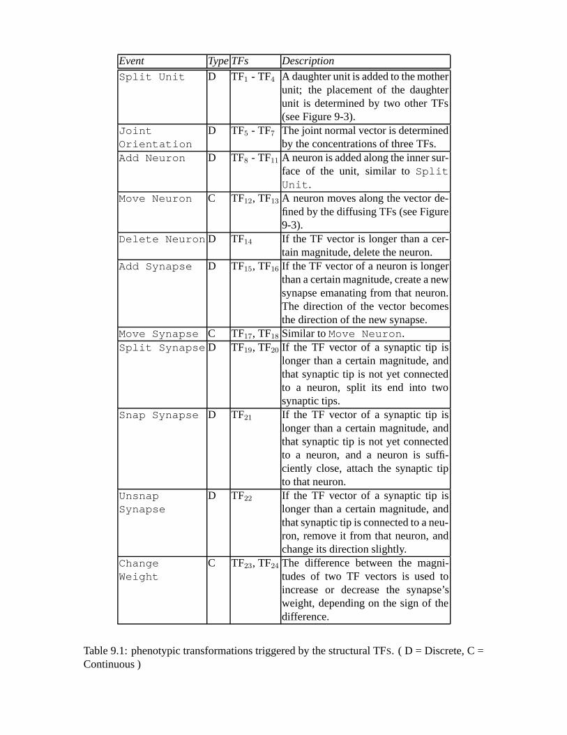
Event TypeTFs Description

Split Unit D TF1 - TF4 A daughter unit is added to the motherunit; the placement of the daughterunit is determined by two other TFs(see Figure 9-3).

JointOrientation

D TF5 - TF7 The joint normal vector is determinedby the concentrations of three TFs.

Add Neuron D TF8 - TF11 A neuron is added along the inner sur-face of the unit, similar toSplitUnit.

Move Neuron C TF12, TF13 A neuron moves along the vector de-fined by the diffusing TFs (see Figure9-3).

Delete Neuron D TF14 If the TF vector is longer than a cer-tain magnitude, delete the neuron.

Add Synapse D TF15, TF16 If the TF vector of a neuron is longerthan a certain magnitude, create a newsynapse emanating from that neuron.The direction of the vector becomesthe direction of the new synapse.

Move Synapse C TF17, TF18 Similar toMove Neuron.Split Synapse D TF19, TF20 If the TF vector of a synaptic tip is

longer than a certain magnitude, andthat synaptic tip is not yet connectedto a neuron, split its end into twosynaptic tips.

Snap Synapse D TF21 If the TF vector of a synaptic tip islonger than a certain magnitude, andthat synaptic tip is not yet connectedto a neuron, and a neuron is suffi-ciently close, attach the synaptic tipto that neuron.

UnsnapSynapse

D TF22 If the TF vector of a synaptic tip islonger than a certain magnitude, andthat synaptic tip is connected to a neu-ron, remove it from that neuron, andchange its direction slightly.

ChangeWeight

C TF23, TF24 The difference between the magni-tudes of two TF vectors is used toincrease or decrease the synapse’sweight, depending on the sign of thedifference.

Table 9.1: phenotypic transformations triggered by the structural TFS. ( D = Discrete, C =Continuous )

Figure 9-1:Morphogenesis and neurogenesis.This figure shows a hypothetical growthprogramme for a simple robot. The upper panel shows the state of the robot at the beginningof growth: two morphological units are attached to each other, all genes are turned off,and two different chemicals that regulate gene expression (TF25 and TF26) are injectedinto the units to initiate growth. In the lower panel, several time steps have elapsed, andsome morphogenesis and neurogenesis has occurred. The states of the genes have divergedin different units (black bars indicate expressed genes; gray bars indicate non-expressedgenes; white tracts indicate non-coding regions). Several neurons (gray filled circles) havebeen created (T = touch sensor neurons,A = angle sensor neurons,M = motor neurons,unmarked = internal neurons). Synapses (arrows) have grown and split, and some haveattached to target neurons. A rotational joint has grown between two units (U2 andU4);the motorized joint is receiving commands from a motor neuron (M in U2), and feedingits current angle into the angle sensor neuron (A in U2). A neural circuit spanning threeunits has grown, starting from the touch sensor inU1, feeding into the motorized joint inU2, and continuing via the angle sensor neuron inU1 into the motor neuron inU4. As U4does not contain a motorized joint, this part of the circuit does not affect behaviour, and isthus neutral, along with the unattached synapses inU2 (the active synapses of the circuitare drawn in bold).

9.2.2 Tasks

Two different fitness functions were employed, one for object manipulation and one forforward locomotion. In the case of the grasping task, the first two units are welded to theenvironment: that is, it is as if the starting two units were welded to a rigid rod that is itselfwelded to the ground plane. For the locomotion task, the agent is able to move freely. Byusing a large object for the grasping task, we indirectly favour agents composed of manyunits, as the agent must grow large enough to reach out for, and grasp the object. Thelocomotion task has seemingly no particular bias towards smaller or larger agents. In both

Algorithm 9.2.1: EVOLVEPOPULATION(gens, popSize)

for p← 1 to gens

do

for g ← 1 to popSize

do

initialize the physical simulation;create two units attached together;copyg into both units;inject TF25 into the first unit;inject TF26 into the second unit;perform the fitness evaluation;assign a fitness value;

sortp in order of decreasing fitness;delete the less fit genomes ofp;copy and mutate selected genomes fromp;copy and cross selected genomes fromp;

Figure 9-2:Pseudocode for the genetic algorithm.The algorithms for growing and eval-uating a robot are shown in Figure 9-5.

cases genomes were evolved to maximize either the function

fg = s + (maxd − closestd) +t∑

j=1

uj∑i=1

tij

or

fl = s + p +u∑

i=1

vi

wherefg andfl are the fitness functions for grasping and locomotion, respectively;s is aninitial shaping function; maxd is the distance betweenU1 and the target object; closestd isthe closest approach of one of the robot’s morphological units to the target object duringevaluation;t is the number of time steps for which the robots are evaluated;uj is thenumber of units comprising the robot at time stepj; tij is 1 if unit i at time stepj is incontact with the target object, and 0 otherwise;p is the forward position, in the horizontalplane, of the robot’s posterior-most3 unit at the end of the evaluation4; andvi is the forwardvelocity of uniti at the end of the evaluation. The shaping functions is necessary in order toaward fitness for robots that do not yet have the phenotypic structures necessary to achievemotion, and thus behaviour:

3The anterior direction is considered the direction towards the target object for the grasping task, and thedirection in which the agent must move for the locomotion task.

4This penalizes agents which passively fall forward, instead of actively moving.

Figure 9-3:Causing phenotypic change: The left-hand panel shows the interior of a mor-phological unit. Chemical transcription factors (TFs) diffuse out from the centre of the unit(black circle). TFs are released by expressed genes lying along the genome (black squaresare expressed genes; gray squares are non-expressed genes). A unit attempts to bud offa daughter unit if TF1 reaches a threshold concentration (see Table 9.1). The placementof the daughter unit is determined by two additional TFs. The concentration of these twoTFs at the centre of the mother unit determine the value of two angles,Θ andΦ, whichdetermine where on the mother units surface the daughter unit is placed. The same proce-dure is used in neurogenesis: one TF triggers the creation of a neuron, and two additionalTFs determine its placement just below the surface of the morphological unit. Aside fromthreshold events such as unit splitting, neuron creation and deletion, and synapse creationand deletion, there are several continuous events, such as neuron and synapse movement.The right-hand panel shows how this is accomplished for neuron movement. For eachneuron in a unit, its change in position is given by a summation of vectors.

Figure 9-4:Genome Architecture: A hypothetical gene is located within the genome bythe presence of a promoter site (Pr), and is flanked by non-coding regions (Nc). Thesix values following the promoter site are translated into the six parameters describingthe gene: this gene is regulated by the 13th regulatory TF (37 − 24 = 13); emits thesecond structural TF when turned on (TF2 aids in the transformationSPLIT UNIT); isinhibited byTF37; emits 0.03 amount ofTF2 when turned on; and is turned on when theconcentration ofTF37 is outside the range[0.23, 0.93].

s =

1 : the robot contains≥ 1 neuron2 : and ≥ 1 sensor neuron3 : and ≥ 1 motor neuron4 : and ≥ 1 synapse5 : and ≥ 1 synapse attached to a neuron6 : and ≥ 1 motorized joint7 : and ≥ 1 angle command sent to a motor8 : and ≥ 1 unit in contact with ground/object0 : the robot contains none of these

Algorithm 9.2.2: EVALUATE ROBOT(evaluationT ime)

procedureUPDATEGRN(u)for g ← 1 to numberOfGenesInGRN

do if the TF regulatingg is presentand within the desired rangethen c(g(TFout), u)← c(g(TFout), u) + αg(TFconc); (*)

if u is touching somethingthen c(TF43, u)← c(TF43, u) + β; (**)

if u contains a motorized jointthen c(TF44, u)← c(TF44, u) + γ(|da(u)− ca(u)|); (**)

for i← 1 to 44

do{

diffuseTFi into u’s neighbours; (diffusion) (*)c(TFi, u)← 0.9c(TFi, u); (decay) (*)

procedureUPDATENEURALNETWORK(u)for n← 1 to numberOfNeurons

do

if TFs indicate transformation(s) onn are imminentthen apply transformation(s) ton; (*)

if n ==SENSORNEURONthen scale the incoming signal to(−1.0, 1.0); (+)elsesum and threshold the values of the incoming synapses;(+)

for s← 1 to numberOfCurrentSynapses

do

propagate neural signal;(+)if TFs indicate transformation(s) tos are imminent

then apply transformation(s) tos; (*)

procedureUPDATEACTION(u)if u contains a motorized jointmj

do

if TFs indicate transformation(s) onmj are imminentthen apply transformation(s) tomj; (*)

da(u)←average of the values of the motor neurons inu (+)scaleda(u) to (−π/2, π/2); (+)translateda(u) into a quantity of torque;(+)apply torque tomj; (+)

f ←sum of the forces and collisions acting onu; (+)update the position, velocity and orientation ofu based onf ; (+)

mainfor t← 1 to evaluationT ime

do

for u← 1 to numberOfCurrentUnits

do

if TFs indicate transformation(s) onu are imminentthen apply transformation(s) tou; (*)

UPDATEGRN(u)UPDATENEURALNETWORK(u)UPDATEACTION(u)

return (fitness);

Figure 9-5:The algorithm to grow and evaluate a robot, given a particular genome.During each timestep of the fitness evaluation, the genetic regulatory network in each unit is updated (UpdateGRN), the neuralnetwork is grown and signals are propagated along it (UpdateNeuralNetwork), and the agent exertssome action on its environment (UpdateAction). Lines with a(*) appended contribute to morphogenesisor neurogenesis; lines with with a(+) appended contribute to the agent’s behaviour; lines with a(**) appendedare those that transduce environmental stimuli into genetic signals.g(TFout) is the TF produced by geneg; g(TFconc) is the amount ofTFout released byg; TF43 and TF44 are the regulatory TFs associated withenvironmental transduction;da(u) is the desired angle of the motor in unitu; ca(u) is the current angle ofthe motorized joint inu; andc(TF, u) is the concentration of theith transcription factor in unitu. α, β andγ are small constants (< 1) that ensure there are no large increases in TF concentration during a single timestep, leading to complete saturation.

The shaping function rapidly leads to functioning robots in early generations, without hav-ing to introduce particular body plans or neural controllers that contain designer bias.

9.2.3 Artificial Growth

Agents are composed of one or more units and zero or more sensor neurons, motor neurons,internal neurons and synapses. At the beginning of robot evaluation, the genome to betested is copied into two attached units (see Figure 9-1). All of the genes lying along thegenomes are initially switched off.

Two different chemical transcription factors (TFs) are injected into the centres of thetwo units, one into the anterior unit, and one into the posterior unit. In the model, all TFsare treated as chemicals, and are subjected to diffusion and decay. TFs diffuse uniformlyoutward from the centre of the unit and concentrations decrease over time (see Figure 9-5). These two maternal TFs (TF25 and TF26) begin to diffuse and decay, and affect theexpression of genes. These genes, if switched on, begin to produce TFs themselves, whichdiffuse and decay out from the centre of the unit as well. Because the two units begin withinjections of different TFs, the regulation of the genes in these units may differ, leadingto differing gene states in neighbouring units. This breaking of symmetry allows artificialevolution to establish major body axes in the developing agent, and not simply produce aclose-packed cluster of identical units (this has been shown to be one of the primary roles ofmaternal TF diffusion during early development [Anderson and Nüsslein-Volhard, 1984] inbiological organisms).

The TFs may directly affect the phenotype of the developing agent: there are 24 pre-defined phenotypic transformations that TFs can initiate. The transformations, and thenumber of TFs required to initiate them, are listed in Table 9.1; the way in which TFsinitiate transformations is illustrated in Figure 9-3.

Because neurons and synapses have particular three-dimensional locations, their localchemical environments—that is, the concentrations of TFs at their location—can be mod-elled simply using vector addition, as shown in the right-hand panel of Figure 9-3. Thisapproach to modelling diffusion has the advantage that concentrations only have to be cal-culated at the positions of neurons, synapses, unit centres and inter-unit boundaries, notacross the entire volumes of the units. Also, objects close to each other experience similarchemical environments, as would be true if the objects existed in a true three-dimensionalchemical environment. At each time step, each neuron and synapse is assigned a TF vector(as shown in Figure 9-3), for each TF that can effect a transformation on it.

Some of the transformations are continuous, in that a change is made during each timestep that the TF concentration for that transformation is above 0. Others are discrete: forSplit Unit andAdd Neuron, this occurs if the concentration of the relevant TF con-centration is above 0.8 at the unit’s centre5; for Joint Orientation, it is the concen-trations of the relevant TFs at the time of joint creation; forDelete Neuron andAddSynapse, it is if the magnitude of the TF vector at the neuron’s location is greater than

5TF concentrations range between 0 (no TF present) to 1.0 (complete saturation).

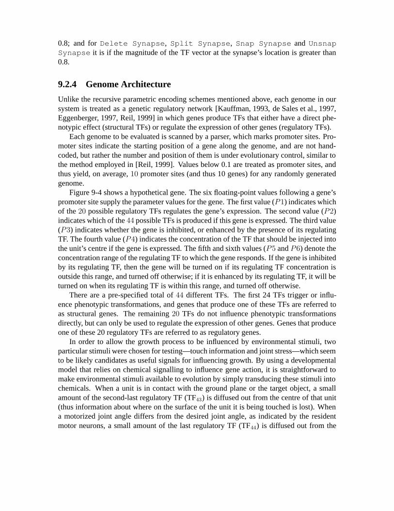
0.8; and forDelete Synapse, Split Synapse, Snap Synapse and UnsnapSynapse it is if the magnitude of the TF vector at the synapse’s location is greater than0.8.

9.2.4 Genome Architecture

Unlike the recursive parametric encoding schemes mentioned above, each genome in oursystem is treated as a genetic regulatory network [Kauffman, 1993, de Sales et al., 1997,Eggenberger, 1997, Reil, 1999] in which genes produce TFs that either have a direct phe-notypic effect (structural TFs) or regulate the expression of other genes (regulatory TFs).

Each genome to be evaluated is scanned by a parser, which marks promoter sites. Pro-moter sites indicate the starting position of a gene along the genome, and are not hand-coded, but rather the number and position of them is under evolutionary control, similar tothe method employed in [Reil, 1999]. Values below 0.1 are treated as promoter sites, andthus yield, on average,10 promoter sites (and thus 10 genes) for any randomly generatedgenome.

Figure 9-4 shows a hypothetical gene. The six floating-point values following a gene’spromoter site supply the parameter values for the gene. The first value (P1) indicates whichof the20 possible regulatory TFs regulates the gene’s expression. The second value (P2)indicates which of the44 possible TFs is produced if this gene is expressed. The third value(P3) indicates whether the gene is inhibited, or enhanced by the presence of its regulatingTF. The fourth value (P4) indicates the concentration of the TF that should be injected intothe unit’s centre if the gene is expressed. The fifth and sixth values (P5 andP6) denote theconcentration range of the regulating TF to which the gene responds. If the gene is inhibitedby its regulating TF, then the gene will be turned on if its regulating TF concentration isoutside this range, and turned off otherwise; if it is enhanced by its regulating TF, it will beturned on when its regulating TF is within this range, and turned off otherwise.

There are a pre-specified total of44 different TFs. The first 24 TFs trigger or influ-ence phenotypic transformations, and genes that produce one of these TFs are referred toas structural genes. The remaining20 TFs do not influence phenotypic transformationsdirectly, but can only be used to regulate the expression of other genes. Genes that produceone of these 20 regulatory TFs are referred to as regulatory genes.

In order to allow the growth process to be influenced by environmental stimuli, twoparticular stimuli were chosen for testing—touch information and joint stress—which seemto be likely candidates as useful signals for influencing growth. By using a developmentalmodel that relies on chemical signalling to influence gene action, it is straightforward tomake environmental stimuli available to evolution by simply transducing these stimuli intochemicals. When a unit is in contact with the ground plane or the target object, a smallamount of the second-last regulatory TF (TF43) is diffused out from the centre of that unit(thus information about where on the surface of the unit it is being touched is lost). Whena motorized joint angle differs from the desired joint angle, as indicated by the residentmotor neurons, a small amount of the last regulatory TF (TF44) is diffused out from the

centre of the unit containing the joint, where the amount of TF released is commensuratewith this difference.

For each time step that a gene emits its TF, the concentration of that TF, at the centreof the unit, is increased by the amount encoded in the gene (which ranges between0.0 and1.0), multiplied by a small constant (α in Figure 9-5). All TF concentrations decay duringeach time step, and diffuse between neighbouring units (seeUpdateGRN in Figure 9-5).All 44 TFs (24 TFs that directly affect the phenotype, and 20 regulatory TFs) share thesame fixed, constant diffusion and decay coefficients.

In our previous models of artificial growth [Bongard and Pfeifer, 2001, Bongard, 2002b],the growth of the agent preceded, and was thus separated from its ability to act in its en-vironment. In our current instantiation, the agent is able to act during growth: this isachieved by allowing the neural network to function (propagating any sensory signals onto motorized joints), while the body and brain are still growing. This is made clear in thepseudocode shown in Figure 9-5, which outlines the three algorithms used to grow andevaluate a robot, given a particular genome.

9.2.5 The Neural Controller


There are two types of sensors that artificial evolution may embed within the units of theagent: touch sensors and proprioceptive sensors. Touch sensor neurons return+1.0 if theunit in which they are embedded is in contact with either the target object or the ground, or−1.0 otherwise. Proprioceptive sensors return a signal in[−1.0, 1.0], commensurate withthe current angle of the motorized joint in that unit, which lies in[− π

2, π

2]. Internal neurons

can also be incorporated by evolution into an agent’s neural network, in order to propagateand transform signals from sensor to motor neurons.

Synapses grow, move and branch out from originating neurons. Synapses are composedof connected series of line segments, each of which has a particular length, direction, andweight, all of which are influenced by gene action (a two-dimensional representation isshown in Figure 9-1). Synaptic tips may or may not attach to target neurons. Propagationof signals along synapses starts at the originating neuron, and passes along each segment ofthe synapse, until it reaches a target neuron. The values of all afferent synapses are summedand thresholded by the target neuron. Signal propagation is given by

s(1)v = no

vs(1)w

s(i+1)v = s(i+1)

w s(i)v

a =y∑

j=1

s(j)v

ntv =

−1 : a ≤ −1

a : −1 < a < 11 : a ≥ 1,

wherenov andnt

v are the values of originating and target neurons, respectively;s(i)w and

s(i)v are the weight and value of theith segment of a synapse, which lie in[−1.0, 1.0],

respectively;y is the number of afferent synapses to a neuron; anda is the activation valuearriving at a neuron. It follows from this that the more segments comprising a synapse, thelonger it takes for a signal to propagate from the originating to the target neuron; the lengthof each segment does not affect propagation time.

Neuronal and synaptic migration (moving from one unit to another) is simulated, sothat long-range neural circuits spanning neighbouring units can be established, if required.If a neuron or synapse moves into the volume defined by overlapping neighbouring units,and its distance to the new unit is closer than the distance to the originating unit, furthertransformations on that neuron or synapse are dictated by the new unit and its neighbours,instead of the originating unit and its neighbours.

9.2.6 Robot Behaviour

The agent achieves motion by actuating its joints. This is accomplished by averaging theactivations of all the motor neurons within each unit, and scaling the value to[− π

2, π

2].

Torque is then applied to the rotational joints such that the angle between the two rigidconnectors forming the joint matches this value. The desired angle may not be achievedif: there is an external obstruction; the units attached to the rigid connectors experienceopposing internal or external forces; or the values emitted by the motor neurons changeover time. Note that failure to achieve the desired angle may be exploited by evolution,and may be a necessary dynamic of the agent’s actions. If a unit contains no motor neu-rons, the rotational joint in that unit is passive. Passive dynamics—behaviour achievedthrough passively swinging joints—is proving to be a useful mechanism for robot design[McGeer, 1990, Frutiger et al., 2002].

The agents reported in this section were evaluated in a deterministic, three-dimensional,physically-realistic simulation package6. During each time step of the evaluation, sensorreadings are taken, the neural network is updated, and the motor commands are translatedinto torques. The torques are passed to the simulator, which updates the positions, velocitiesand orientations of each of the agent’s units. The updates are also affected by simulatedexternal forces such as gravity, inertia, friction and collision or contact with the groundplane7. Each agent was grown and evaluated for 500 time steps.

6Open Dynamics Engine,http://opende.sourceforge.net.7By evaluating the agent in a physically realistic simulation, agents can evolve to take advantage of their

environment, such as using gravity and momentum to move non-actuated joints in a useful manner. Also, itmay be easier to translate evolved solutions into real-world robots.

9.3 Results

Using the fitness function for grasping (fg), 20 independent evolutionary runs were per-formed, starting with different random starting populations. Three independent runs wereperformed using the fitness function for locomotion (fl).

Most of the populations evolved for grasping were able to produce a morphology thatcould reach the target object, and most were able to keep fairly constant contact with thesphere, including several strategies to slide different parts of the body across the object.Figure 9-6 shows the best solutions from six of the evolved populations, and the best solu-tions produced by the three populations evolved for locomotion.

There are two immediate trends that can be seen in Figure 9-6: first, that the best agentsfor grasping tend to be much larger than those for the locomotion task; and second, thatrepeated morphological structure is apparent, especially in the agents in panelsb andf. Thefirst trend can be explained purely from the viewpoint of the task environment: because thegrasping agents are fixed, they must grow large enough to reach the target object, and thenbe able to manipulate this large object. The locomoting agents, by contrast, do not need tobe large or complex in order to move forwards. The reason for repeated structure, however,cannot be explained simply by the task. Previous results [Bongard and Pfeifer, 2001] havesuggested that these repeated structures are a product of gene action; the same subsets ofgenes are being expressed in units which produce similar structures.

9.3.1 Properties of Evolved Genomes

In order to clarify the relationship between phenotypic structure, behaviour and gene ac-tion, the genomes of the evolved populations were analyzed. Figure 9-7 shows the genetichistory of one of the evolved populations. In the early generations, the genome rapidlylengthens to approach the maximum length of 1000 floating-point values. The number ofgenes also increases during this period, but there is no apparent change in gene density, norin the ratio between regulatory and structural genes over evolutionary time.

These trends are shown more clearly in Figure 9-8, which plots various properties ofthe evolved GRNs against the fitness of the agent. The fitness curves in Figure 9-8 showthe normalized fitness of the best agent in the population for that generation. Due to thelarge discontinuous jump in fitness once agents are able to fulfil the criteria of the shapingfunction, the fitness values of the best agents from each generation are normalized: themost fit agent from the first generation is assigned a normalized fitness value of 1; once amore fit agent appears in a subsequent generation, that agent is assigned a fitness value of2; and so on. These normalized fitness values are used only for illustrative purposes: theyindicate periods of evolutionary improvement, as well as fitness plateaus.

Figure 9-8a plots the normalized fitness curve of best agents against the number ofgenes contained in their genomes. Figure 9-8b plots the fitness curve against the fractionof non-coding regions of the genome, which is calculated usingl − 7g, wherel is thelength of the genome,g is the number of genes contained in the genome, and each gene

a b c

d e f

g h i

Figure 9-6:Sample morphologies from the two tasks.Panelsa to f show examples of thebest agents evolved for the grasping task, and panelsg to i show the best agents evolved forthe locomotion task. Dark gray spheres indicate units that contain motorized joints; whitespheres indicate units that are welded to their neighbouring units. The target object can beseen to the upper left of the grasping agents. All images were taken att400, near the end ofevaluation.

is composed of 7 values (6 parameters plus the promoter site). Figure 9-8c plots fitnessagainst the fraction of genes contained in the genome that are regulatory genes.

Figure 9-8d plots fitness against the average number of genes contained in a genefamily for that genome. Genes are considered to belong to a family if they have at leastone parameter (or promoter site) value equal to each other. Since the floating-point valuesare accurate to±10−4, and only random replacement is allowed for point mutations, theprobability error that two genes have independent origins and at least one equal value is

a0 200 400 600 800 1000

0

10

20

30

40

50

60

70

80

90

100

Genome length

Gen

erat

ion

b c d

Figure 9-7:The genetic history of an evolved population.In a, the horizontal axis givesthe length of the genome, measured in numbers of floating-point values. The vertical axisgives the generations of evolutionary history. Each genome shown is that taken from themost fit agent appearing in the population during that generation. The line indicates tractsof non-coding regions; the light gray boxes indicate structural genes; the dark gray boxesindicate regulatory genes.b, c andd show the adult morphologies (at t400) of the bestagents taken from generations 30, 35 and 40, in which a drastic change in body plan wasobserved.

less than1/10000 = 0.0001, which we regard as negligible. As can be seen, the number ofgenes and participation in a gene family changes considerably at the early in evolution, andthen remains fairly constant,whereas the fractions of non-coding regions and regulatorygenes remain relatively constant throughout evolution.

Each of the four genetic measures was calculated for the most fit agent from the firstgeneration, and the most fit agent from the last generation, for each of the 20 populationsevolved for the grasping task as well as the three populations evolved for the locomotiontask, and are reported in Figure 9-9.

9.3.2 Environmental Shaping of Growth

In order to determine whether the environmental stimuli are appropriated by evolution toguide the developmental programmes of the agents, lesion experiments were performed.The use of lesion studies is a standard technique in neuroscience [Young, 1970], embry-

a0 20 40 60 80 100

0

5

10

15

20

25

30

35

0

10

20

30

40

50

60

70

Num

ber of genes

Generation

Fitn

ess

b0 20 40 60 80 100

0

5

10

15

20

25

30

35

0

0.14

0.29

0.43

0.57

0.71

0.86

1

Non−coding R

egions / G

enome Length

Generation

Fitn

ess

c0 20 40 60 80 100

0

5

10

15

20

25

30

35

0

0.14

0.29

0.43

0.57

0.71

0.86

1

Fraction of R

egulatory Genes

Generation

Fitn

ess

d0 20 40 60 80 100

0

5

10

15

20

25

30

35

0

0.4

0.8

1.2

1.6

2

2.4

2.8

Average F

amily S

ize

Generation

Fitn

ess

Figure 9-8:Changes to evolved GRNs: The thin lines represent the normalized fitnessesof the best agents from each generation for one of the populations evolved for grasping, andcorrespond to the left-hand vertical axis. The GRN properties are plotted using the thickline, and correspond to the right-hand vertical axis.a plots fitness against the total numberof genes contained in the genome,b plots fitness against the fraction of non-coding geneticmaterial,c plots fitness against the fraction of regulatory genes among the total number ofgenes, andd plots fitness against the average number of genes contained in a gene family.Circles indicate the values of the GRN properties for the agents from generations 30, 35and 40.

ology [Hamburger, 1988, Hill and Sternberg, 1993], and more recently, developmental ge-netics (for example [Lewis, 1992]). Lesioning involves the selective removal or disruptionof some part or dynamic of a growing organism, and measuring the effect on either itsgrowth programme, adult phenotype or behaviour. Lesioning has recently begun to beused for studying artificial neural networks by Aharonovet al [Aharonov et al., 2001]. Ina previous study we lesioned evolved neural networks to determine how sensory infor-mation in a simulated agent was being used to drive behaviour [Bongard, 2002a], and in[Bongard, 2002b] we systematically lesioned genes in evolved GRNs to determine howgene action was integrating and/or dissociating morphogenesis and neurogenesis.

In order to determine whether evolution appropriated the environmental stimuli madeavailable, evolved agents were re-grown, with the transduction of environmental stimuli

a0 5 10 15 20

0

10

20

30

40

50

60

70

80

Population

Gen

es

b0 5 10 15 20

0

0.1

0.2

0.3

0.4

0.5

0.6

0.7

0.8

0.9

1

Population

Non

−co

ding

Reg

ions

/ G

enom

e Le

ngth

c0 5 10 15 20

0

0.1

0.2

0.3

0.4

0.5

0.6

0.7

0.8

0.9

1

Population

Fra

ctio

n of

Reg

ulat

ory

Gen

es

d0 5 10 15 20

0

0.5

1

1.5

2

2.5

3

Population

Ave

rage

Fam

ily S

ize

Figure 9-9: GRN changes across populations: Each of the four genetic measures arecomputed for the best agent from the first and last generations in each of the 20 populationsevolved for grasping, and the three populations evolved for locomotion. The black bars de-note the genetic measures for the agents from the first generation (for both the grasping andlocomotion tasks), the light gray bars denote the genetic measures for the agents from thelast generation (for the grasping task), and the dark gray bars denote the genetic measuresfor the agents from the last generation (for the locomotion task).a plots the total number ofgenes contained in the genome,b plots the fraction of non-coding genetic material,c plotsthe fraction of regulatory genes among the total number of genes, andd plots the averagenumber of genes contained in a gene family.

into their representative chemicals suppressed8. Note that this does not imply that thosetwo chemicals, TF43 and TF44, cannot influence gene action: there may be genes thatproduce these chemicals. It is simply the environmental source of these chemicals that issuppressed, not their genetic source (if any). Figure 9-10 shows the effect of this lesion onthe most fit agent taken from the population documented in Figure 9-8.

8Our usage of the term ’lesion’ is quite broad, in that there is no actual structure that is being disabledhere, but rather a process: in this case, transduction.

Figure 9-10:Effect of suppressing environmental transduction during growth. Theupper row shows the growth of the most fit agent from one of the evolved populations forgrasping. Still frames are taken at time steps 10 (t10), t20, t50, t100, t200 andt400. The lowerrow shows the effect of re-growing this agent, but suppressing environmental stimuli frombeing transduced into the two corresponding chemicals TF43 and TF44.

Figure 9-10 clearly indicates that in the latter stages of growth, suppressing this trans-duction does affect the growth programme, indicating that artificial evolution has exploitedthese environmental cues to guide growth. In order to trace this appropriation back throughthe environmental history of this population, the best agent from each generation was le-sioned. In fact a total of22 lesions were performed for each of these agents. The first 20lesions involved suppressing genes which produce one of the 20 regulatory TFs (TF24 toTF44). The first lesion suppressed all genes that produced TF24 during growth, the secondlesion suppressed all genes that produced TF25 during growth, and so on. The second-last lesion corresponded to suppressing just the transduction of joint stress into TF43, andthe last lesion corresponded to suppressing just the transduction of touch information intoTF44. The results of these lesions are reported in Figure 9-11 for two of the populationsevolved for grasping.

This set of lesion experiments was then performed on the other 19 populations evolvedfor grasping. The probability that a particular lesion would have an effect on fitness for thebest agent from each generation was calculated. The results of this calculation are reportedin Figure 9-12.

As can be seen in Figure 9-11a, the genetic origin of TF43 precedes the environmentalorigin of TF43 as a factor guiding growth: barring genes from producing TF43 begins tohave an effect in generation 25, and suppression of the environmental transduction beginsto have an effect in generation 68. In the case of TF44, the environmental origin precedes thegenetic origin in affecting growth: suppression of the environmental transduction of TF44

has an effect on fitness beginning at generation 19, and suppression of genes producingTF44 has an effect on fitness beginning at generation 73. In Figure 9-11b, however, neither

a 0 10 20 30 40 50 60 70 80 90 1000

5

10

15

20

Generation

Lesi

oned

TF

b 0 10 20 30 40 50 60 70 80 90 1000

5

10

15

20

Generation

Lesi

oned

TF

Figure 9-11: Lesion effects on evolved agents.Panela corresponds to the populationwhich evolved the agent shown in Figure 9-10. Panelb corresponds to the population whichevolved the agent shown in Figure 9-6c. Each column corresponds to the lesion effects onthe most fit agent present in the population at that generation. A filled square indicates thatthat particular lesion had an effect on fitness, and thus contributed to the growth of thatagent. Blank areas indicate that that particular lesion did not affect the fitness of that agent,and thus did not contribute to the growth of that agent. Each row corresponds to a particularlesion experiment. The lowest row corresponds to suppressing genes that produce TF24

during growth, the second row corresponds to suppressing genes that produce TF25 duringgrowth, and so on. The row marked with a filled diamond corresponds to suppressinggenes that produce TF43 during growth. The row marked with a filled triangle correspondsto suppressing the transduction of joint stress into TF43. The row marked with a filled circlecorresponds to suppressing genes that produce TF44 during growth. The row marked witha filled square corresponds to suppressing the transduction of touch information into TF44.

environmental cues are used to guide growth. However, both TF43 and TF44 are producedby genes, and are used as signals to guide growth, as lesioning the genetic origin of theseTFs has an effect on fitness starting early in evolution (around generation 20 for TF43 andgeneration 30 for TF44). Figure 9-13 shows whether and when the two environmental cuesare appropropriated by evolution, for the 20 populations evolved for grasping.

0 10 20 30 40 50 60 70 80 90 1000

5

10

15

20

Generation

Lesi

oned

TF

Figure 9-12:Generalized lesion effects across all evolved populations.The 22 lesionexperiments were performed on the best agent from each generation, for all 20 populationsevolved for grasping. The probability that a particular lesion would have an effect on fitnesswas calculated for each lesion, for each generation. The darker regions indicate greaterprobability, such that black squares correspond to particular lesions that had a fitness effecton all of the best agents extracted from the 20 populations, for that generation. The lowestrow corresponds to suppressing genes that produce TF24 during growth, the second rowcorresponds to suppressing genes that produce TF25 during growth, and so on. The rowmarked with a filled diamond corresponds to suppressing genes that produce TF43 duringgrowth. The row marked with a filled triangle corresponds to suppressing the transductionof joint stress into TF43. The row marked with a filled circle corresponds to suppressinggenes that produce TF44 during growth. The row marked with a filled square correspondsto suppressing the transduction of touch information into TF44.

9.4 Discussion

Figure 9-6 shows that our combined model of artificial development and evolution is ableto generate varied, and complex agent phenotypes to achieve the desired task. Specifically,all six of the evolved agents for grasping shown in Figure 9-6 achieve similar fitness values.

However, Figure 9-7 shows that during evolution, in some cases there are drastic changesin phenotype (the morphologies of the best agents from generation 30, 35 and 40 are givenas examples) which are the result of smallchanges in the genotype.

The genomes for these agents (Figure 9-7a) seem very similar in terms of the numbersand distribution of the structural and regulatory genes. This indicates that the phenotypicchanges must be attributable to changes in gene regulation, rather than additional genes, orradically different genomes (such as would be the case if the best agents from generations30, 35 and 40 were not closely related).

Figure 9-8 indicates that there are periods during which there is no improvement in thefitness of the best agent (denoted by the fitness plateaus near the end of the evolutionaryrun). This indicates that the best agents in the population for those generations have identi-cal phenotypes, insofar as it relates to fitness (there may be differences among unused neu-ral structure between these agents). However, the GRNs contained in these phenotypicallyidentical agents do show differences: this is indicated by the small changes in GRN prop-

a0 5 10 15 20

0

10

20

30

40

50

60

70

80

90

100

Population

Gen

erat

ion

b0 5 10 15 20

0

10

20

30

40

50

60

70

80

90

100

Population

Gen

erat

ion

Figure 9-13:Onset of evolutionary appropriation of environmental stimuli. Panelaoutlines the role of TF43 in guiding growth for the 20 populations evolved for grasping.The diamonds indicate the first generation in which the growth of the most fit agent inthe population at that time was influenced by genetic production of TF43. The trianglesindicate the first generation in which the growth of the most fit agent in the populationwas influenced by environmental production of TF43. The thick lines indicate the lengthof evolutionary time until the other source of TF43 was also exploited to guide growth.Thick lines that do not terminate with a symbol indicate that the other source was neverexploited. Panelb outlines the role of TF44 in guiding growth. The circles indicate the firstgeneration in which the growth of the most fit agent in the population was influenced bygenetic production of TF44. The squares indicate the first generation in which the growthof the most fit agent in the population was influenced by environmental production of TF44.The thick lines indicate the length of evolutionary time until the other source of TF44 wasalso exploited to guide growth. Thick lines that do not terminate with a symbol indicatethat the other source was never exploited. The thin lines indicate those populations forwhich neither of the sources of TF44 were made use of to guide growth.

erties during these periods. This indicates that mutations are accumulating in the neutralparts of the genome, and may indeed be contributing to subsequent fitness improvements.

In addition to the phenotypic variability and genotypic similarity seen within an evolv-ing population, a similar characteristic appears when comparing genotypic properties acrossgenerations: Figure 9-9 shows that the evolved GRNs in the populations for grasping andlocomotion are similar in several ways. They all contain roughly the same number of genes,starting with around 10 genes in the best agent from the first generation (as expected, giventhe probability of promoter sites in random genomes), and climbs to around60± 15 in thelast generation (Figure 9-6a). However the presence of around 60 genes is likely an artefactof the imposed maximum genome length: what is important to note is that the numbers ofgenes in highly fit genomes is relatively constant across populations, and that this numberdoes not change much during long periods of subsequent evolutionary improvement (suchas between generations 40 and 100 for the population shown in Figure 9-8a).

a b

Figure 9-14:The internal neural circuits of a sample agent. aprovides a magnificationof the centre of the agent shown in its entirety in Figure 9-6b. b shows the internal neuralstructure of this part of the agent. Large black circles indicate the centres of morphologicalunits; black lines indicate connected neighbouring units; smaller circles indicate neurons;dark gray lines indicate synapses that connect to neurons; light gray lines indicate uncon-nected synapses.

There also appears to be very little change in the fraction of non-coding regions, despitethe large increases in genome length and gene number, which remains quite close to one-half of the total values contained in the genome (Figure 9-6b).

However, it is possible that significant numbers of genes do not contribute to the de-velopmental programme, either because: they are never switched on; they produce TFs incontexts in which those TFs do not cause any phenotypic transformations; or they producephenotypic structures that do not affect behaviour, and thus fitness, such as motor neuronsin units that do not contain motorized joints, or synapses that do not connect to a targetneuron. Indeed most of the agents contain significant amounts of neural structure that doesnot contribute to behaviour, as shown in Figure 9-14: note the many unconnected neuronsand synaptic branches that do not innervate any neurons.

Further lesion studies are planned on the evolved GRNs in which individual genes arelesioned, and their effects on behaviour are measured. There is a growing body of work inthe evolutionary computation literature that is concerned with the beneficial role of neutral-ity in evolutionary algorithms [Barnett, 1998, Ebner et al., 2001, Lones and Tyrrell, 2002].Analysis of these four levels of neutrality present in our model (non-coding regions, unex-pressed genes, expressed genes that do not grow phenotypic structure, expressed genes thatgrow unused phenotypic structure) may contribute to understanding the role of neutralityin artificial evolution.

In contrast to the constancy of the amount of non-coding regions, evolution rapidlyorganizes genomes into collections of gene families, as indicated by Figure 9-9d. Earlyevolved genomes contain independent genes (the average number of genes in a gene ‘fam-ily’ is 1), and at the end of evolution tend to contain gene families with an average of

two genes per family. The presence of gene families indicates that evolution relies ongene duplication in all of the evolved populations, irregardless of the fitness function. Itseems possible that this is due to the evolutionary dynamic observed in biological species,in which gene duplication produces one or more genes that then experience less selectiveconservation, as their function is redundant, and subsequent divergence in sequence allowsfor the evolution of more elaborate phenotypes (examples include the hemoglobin family inhumans [Ohno et al., 1986], and elaboration of body plans [Meyer, 1998] and neural differ-entiation [Glover, 2001] due to the duplication of the Hox gene family in higher animals).

These trends seen in our evolved GRNs seem to be conserved across all 20 populationsevolved for grasping, and even for the separate task of locomotion. This indicates thatdespite the varying phenotypes, selection pressure shapes artificial genetic regulatory net-works in particular ways, such as increasing numbers of genes, not reducing nor inflatingnon-coding regions, and creating gene families. Furthermore, these trends are independentof the starting random population, and are also independent of the particular fitness func-tion: the GRN architectures are not an artefact of historical accident during evolution, northe particular task for which the population is evolved.

The fraction of regulatory genes, however, does show large variation from one evolvedpopulation to the next (Figure 9-6c): the reason for this is not immediately clear.

These findings mirror those occuring in developmental genetics, in which it is be-coming increasingly clear that genomes across species are more highly conserved thanpreviously thought [Ferrier and Holland, 2001]. More specifically, species seem to sharecommon gene regulation hierarchies, in which inter-species variability lies primarily inthe different phenotypic structures produced by these hierarchies (for an overview see[Gehring and Ruddle, 1998]).

The morphological differences, and thus fitness differences, between the wild typeagent and the same agent regrown while suppressing the transduction of both touch in-formation and joint stress into regulatory chemicals indicates that the environment plays arole in guiding growth for this particular agent (Figure 9-10). Note that for this particularagent, the phenotypic effect of suppressing trandsuction is local: in the lesioned agent, theanterior appendage does not grow as long as in the wild type agent, and the left-hand ap-pendage is much longer, but the rest of the body is unaffected (note also that these effectsonly begin to appear after t100).

However, the result of systematic lesion experiments shown in Figure 9-11 indicate thatnot every population appropriates these environmental cues to guide growth. Figure 9-11a indicates that this population uses both cues, whereas another population (Figure 9-11b)appropriates neither. This indicates that the environment is a useful, but not a necessaryfactor for evolutionary success for this task.

Figure 9-11 also indicates how the 20 different regulatory TFs are incorporated into thegrowth programmes. Genomes from early generations only rely on one or two regulatoryTFs, or in the case of the population shown in Figure 9-11b, no regulatory TFs at all9 The

9This is possible if genes are inhibited by the presence of their regulatory TF; if that TF is not present, thegene is always on.

population in Figure 9-11a eventually relies on all 20, whereas the population shown inFigure 9-11b only uses 5. This trend towards reliance on an increased number of regu-latory TFs can be seen for all populations in Figure 9-12: the probabilities that any oneof the regulatory TF will play a role in growth increases over evolutionary time (the rowsgradually darken from left to right).

Further, it can be seen that joint stress is used more often in the evolved solutions thanthe touch information (indicated by the darker band corresponding to the upper dark grayarrow, as compared to the band indicated by the upper light gray arrow).

Figure 9-13a shows that 17 of the 20 populations eventually employ joint stress infor-mation to guide growth (noted by the 17 triangles in the figure). Of these 17 populations,five populations never contain genes that produce the TF associated with this environmen-tal stimuli, TF43, in a situation in which it plays a role in guiding growth (indicated by thecolumns that only contain a triangle in the figure). Seven populations contain agents whosegrowth programmes are influenced by genetic production of TF43 before the environmen-tal signal inherent in this chemical is also exploited to guide growth (diamonds lie belowthe triangles in the figure). The remaining five populations contain agents that originallyrespond to the environmental origin of TF43, and later respond to the genetic origin of TF43.

Figure 9-13b shows that 11 of the 20 populations employ touch information to guidegrowth, as opposed to the 17 populations that employ joint stress. Thus, it seems possiblethat joint stress information is more useful as an environmental signal guiding growth thantouch information is, but more populations would have to be evolved in order to confirmthis statistically. Also, Figure 9-13b indicates that some of the 11 populations that employtouch information to guide growth never rely on the genetic origin of the TF associatedwith this stimuli (TF44), some populations rely on it before the environmental stimuli isappropriated, and some rely on the environmental source of TF44 before they rely on thegenetic source of it.

Figure 9-13 thus shows that evolving populations can combine both internal (geneti-cally produced) and external (environmentally produced) signals to guide growth, and thusan agent can adaptively change during its lifetime in response to both its internal state andexternal environment. Hinton & Nowlan [Hinton and Nowlan, 1987] showed that lifetimelearning, combined with genetically encoded information, could beneficially transform thefitness landscape of a learning task, compared to a similar regime in which no learningtook place. The evolutionary dynamic of genetic assimilation [Waddington, 1942] was im-plicated as the reason for this increased evolvability. Genetic assimilation—and a wellknown variant, the Baldwin Effect [Harvey, 1997]—is the process by which a phenotypicchange caused by environmental factors eventually becomes genetically programmed overevolutionary time. In our model, learning is replaced by a more general dynamic: environ-mental effect on morphogenesis and neurogenesis, in which growth and behaviour occurthroughout the lifetime of the agent. Future experiments are planned, similar to the method-ology presented in Hinton & Nowlan’s work, to demonstrate that the lifetime plasticity ofthe agents in our model does indeed smooth the fitness landscape and increase evolvabilityof the system.

9.4.1 Limitations and Opportunities

Despite the host of biological details implemented in this model, there are many abstrac-tions inherent in the system as well. It is important to note that the goal of this work is tobuild a system that can continually evolve more sophisticated robots, with morphologiesand neural controllers that meet the given task, and not to serve as a biological model. Forexample, there is an upper limit (300) on the numbers of morphological units comprisingan agent. This limit, in addition to the numbers of motorized joints, neurons and synapses,was imposed purely for computational reasons: as physical simulation sophistication andcomputing power increase, these limits can be raised. However even with a maximum of300 units, some large agents exhibit complex curved three-dimensional shapes (Figure 9-6a, c ande), distinct from the blocky, segmented body plans seen in other evolved robots[Sims, 1994, Ventrella, 1994, Adamatzky et al., 2000, Hornby and Pollack, 2002]. Thus inour model the addition or deletion of one or a few units through mutation has a small be-havioural effect. As the probability of a mutation having a deleterious effect is proportionalto the magnitude of its phenotypic effect [Arthur, 2000], it is predicted that as the maxi-mum number of modules allowed for growing an agent increases, the evolvability of thesystem will also increase. This hypothesis will be the focus of future experiments.

Another limitation is the maximum genome length. Most populations exhibited a simi-lar dynamic, which was a rapid increase in genome length until it approaches the maximum,followed by length stabilization, in which subsequent evolutionary change occurs throughchanges in gene regulation, not gene number. It may be possible to remove the require-ment of a maximum genome length by incorporating some aspect of metabolism, in whichgenome copying incurs a metabolic cost, commensurate with the length of the genome.Other limitations of the GRNs, such as the stipulation that genes are regulated by only oneTF, could easily be relaxed. It would also be straightforward to add to the available sensortypes, environmental stimuli and inter-unit joint types.

The shaping function also introduces certain designer biases into the evolved agents,such as the requirement that all agent behaviour is based on sensory input, and not purelyon internally generated oscillatory signals. Other experimental design choices, such as thegrasping and locomotion tasks, as well as the external environment itself, may introducefurther that are not immediately obvious.

It would be useful to iteratively relax each of the above-listed constraints. In this way,the current experiments would serve as a control case, and any observed increase in evolv-ability could then be attributed to the particular detail introduced into the model. Thiswould aid in the difficult enterprise of attempting to relate evolutionary performance to thevarious dynamics inherent in this relatively complex model.

9.5 Conclusions

We have here introduced a model that combines artificial growth and artificial evolutionof simulated, embodied robots. This model has been shown capable of evolving robots

for object grasping, and forward locomotion. Further, it has been shown that increases inphenotypic complexity caused by evolution are often accomplished not through increasesin genome size or gene count, but in modifications of gene regulation. This is a desirablefeature of evolutionary computation, as it suggests the presence of modularity: one or a fewregulatory genes orchestrate larger numbers of structural genes. It also suggests that thismodel is scalable: increasingly complex phenotypes can be evolved to meet increasinglychallenging tasks, without an attendant increase in the dimensionality of the genetic searchspace brought about by an increase in genome length or gene number.

Further, this model easily allows environmental cues to be made available for the di-rection of growth, which has not yet been accomplished in recursive encoding schemes forthe evolution of both the brains and bodies of simulated robots. Moreover, evolution is notforced to use the environmental stimuli implemented in the model: it need only be used ifit is useful for the particular task.

Such environmental accomodation would be exceedingly difficult in direct encodingschemes. It may be possible to formulate a recursive encoding scheme that incorporatesenvironmental stimuli by using a variant of open L-systems, but all of the recursive encod-ing schemes proposed so far for the evolutionary design of robots produce a fixed, adultphenotype, that is evaluated only after growth is complete. In constrast to recursive encod-ing schemes, our model combines growth and behaviour evaluation over the lifetime of theagent, and allows growth to be guided during this lifetime by either genetic signals, envi-ronmental cues, or some combination of both. This property has been widely documentedin biological organisms, and has been shown to increase evolvability in evolutionary algo-rithms in the case of learning: this suggests that such developmental models are worthy ofstudy for the advancement of evolutionary computation.

Future experiments, based again on lesion studies, are planned in order to further inves-tigate the role of neutrality in this model, and whether our model does exhibit, or is capableof exhibiting genetic assimilation, and how this relates to the evolvability of the system. Itis also hoped that as robots evolve to perform increasingly challenging tasks, the resultantincreased sophistication of neural structure will provide insights into the transition fromartificial evolution to artificial intelligence.

Chapter 10

Argument

This chapter provides the main discussion and interpretation of the results found in thepreceding eight chapters. We assume that the reader is familiar with the main results inthose chapters; each chapter contains a published paper dealing with a specific aspect ofthe artificial evolution of robots. Here we draw these results together, to outline the maindrawbacks of standard evolutionary robotics, and how the field can be enriched by incorpo-rating morphological—and morphogenetic—considerations into the design process. Thisargument has the following structure:

• Chapter 2 documents a standard evolutionary robotics experiment performed in sim-ulation. The purpose of these experiments is to highlight some of the limitationsof such an approach. However, in that chapter I first show that there are severalhypotheses and algorithm enhancements that can be tested with such an experimen-tal regime: that is, evolving behaviours for a virtual robot with a fixed body plan.As an example, I demonstrate (through lesion studies used as an analytic tool) thatthe genetic algorithm used incrementally integrates the different sensory modalitiesavailable, as opposed to integrating them at the beginning of evolution, and subse-quently improving the behaviour by modifying that integration. However, the factthat the morphology was fixed, and not under evolutionary control, raises severalquestions, such as whether the fixed antennae of the agent limited its ability to trackthe chemical concentration landscape.

• Chapter 3 outlines a methodology for addressing these types of questions. In theexperiments described there, a set of 10 virtual robots with fixed, but differing bodyplans contain the same neural controller, and are evolved to perform the same tasks.Any observed differences in evolutionary performance can thus be attributed to mor-phological differences, and we can then explicitely state what types of body plansare well suited (or not well suited) for particular tasks. However, this methodologyrequires the experimenter to manually modify the fixed body plans in order to assessdifferences between them.

133

• Chapter 4 introduces a set of experiments performed on a generic body plan—abipedal agent—in which the genetic algorithm has some ability to modify the mor-phology. This allows automates the search for a good fit between robot morphology,neural control and behaviour. Two sets of experiments are described, in which thegenetic algorithm can slightly and greatly modify the robot’s mass distribution, re-spectively. It is demonstrated that despite the increased dimensionality of the searchspace with the inclusion of the morphological parameters, the ability of artificialevolution to discover useful behaviours is increased. However in this chapter theexperimenter is still required to set the generic body plan manually.

• Chapter 5 introduces a first set of experiments in which artificial evolution has deepercontrol over both the neural network controller and the morphology. Here, the net-work architecture nor the body plan is fixed by the experimenter. A direct genotype tophenotype transformation is employed to investigate one particular interdependencybetween morphology, control and behaviour: the relation between bilateral symme-try and locomotive efficiency. As described in this thesis, though, there are severallimitations to a direct encoding scheme.

• Chapters 6, 7, 8 and 9 introduce a morphogenetic genetic algorithm, called artificialontogeny, that allows for the growth of the robot’s body and brain together. In theseexperiments I show that this developmental encoding scheme (which relies on differ-ential gene expression) has several benefits over both direct and recursive encodingschemes. In chapters 6 and 9 shows that such an encoding dissociates the length ofthe genome from the complexity of the robot’s phenotype. Chapters 7 and 8 providedetailed analysis as to what genetic regulatory network architectures lead to usefulbehaviours. This work provides insight into how to better tune this model such thatuseful behaviour is achieved more often. Finally, in chapter 9 we show that artifi-cial ontogeny has one major advantage over other developmental encoding schemes:our model allows the environment to shape the developmental processes of the robotduring its lifetime.

10.1 Standard Evolutionary Robotics

Chapter 2 presents a relatively standard evolutionary robotics experiment, which quiteclosely follows the flow outlined in Figure 1-3. First, a task is chosen: in these experi-ments, the task is for a robot to approach a chemical point source that has diffused throughthe environment. That is, the robot must evolve to perform chemotaxis. The robot existsin a three-dimensional environment, but the chemical diffuses through a two-dimensionalplane above and parallel to the flat ground plane (see Figure 2-2).

Second, a robot must be constructed that will at least have the potential to solve thegiven task. A quadrupedal agent was chosen, and a pair of chemical sensors were includedso that the robot could extract information from the two-dimensional chemical environ-

ment. Touch sensors were also placed in the feet, and angle sensors were placed on the legjoints. Motors were placed on the leg joints, but the two antennae containing the chemicalsensors were welded to the front of the robot’s body. This is but one of a host of relativelyarbitrary morphological design considerations that must be made during such experiments.For example, it is not clear whether the task would be easier or more difficult to solve if therobot were equipped with movable antennae.

Next, a neural controller must be chosen for the given robot. A relatively standard fully-connected, feed-forward neural network was chosen, in which the sensors feed values intothe input layer, and values arriving at the output layer are passed to the motors as desiredangle commands (see Figure 2-3 and Chapter 2 for a more detailed description of the neuralcontroller). Finally, an algorithm must be employed to optimize the synaptic weights of thecontroller such that the robot performs (or becomes better at) the desired task. Irregardlessof whether a learning or evolutionary scheme is used, the designer must quantify robotbehaviour, such that larger (or smaller) values indicate the robot is performing the giventask better (or worse)1. This is necessary so that the computer can automatically measurehow well the robot is performing at the given task (in learning, this is known as theteachingsignal; in evolutionary algorithms, this is known as thefitness function).

A standard genetic algorithm is employed to optimize the synaptic weights; the fitnessfunction is determined to be the final distance of the robot from the chemical point source.The fitness function is actually a sum of four distances, because the robot is placed infour environments, with the chemical point source placed in different locations in eachenvironment. It follows that lower fitness values indicate that the robot is able to walkcloser to each of the chemical point sources in the four environments.

The genetic algorithm then iteratively applies weights to the synapses of the robot’scontroller, and the robot is tested in the task environment. A series of 10 independentevolutionary runs were performed; that is, a different population of 200 random genomeswere generated, and each population was evolved for 50 generations. It was found thatall of the 10 populations produced successful chemotacting behaviours (the behaviour ofthe most successful agent is depicted in Figure 2-5). Often, this is the end of an evolu-tionary robotics experiment: a particular evolutionary scheme is shown to be better thana competing scheme by evolving better solutions. However, in this set of experiments ad-ditional analysis was performed in order to gain insight into how the evolutionary processwas generating successful controllers. This was accomplished by performing a series oflesion studies.

10.1.1 Lesioning PerformedIn Silico

Throughout this thesis, lesion experiments are performed in order to understand how anartificial evolutionary process has produced a particular solution. Lesion experiments in-volve the removal or disruption of part of a system, and measuring the effect. If the lesion

1Whether increasing or decreasing values indicate better performance is not important; what is importantis that different values indicate differing performance.

has an effect on the normal operation of the system, then it can be concluded that the le-sioned part of the system plays some role in the functioning system. This technique has itsroots in neuroscience, or more particularly neuropsychology. Paul Broca described how aparticular form of language aphasia was caused by damage to a particular part of the brain,which later became known as Broca’s Area [Schiller, 1979]. Lesioning also has its roots inneuropathology, as the very term ’lesion’ implies damage to an organ. The replacement ofmuskets by rifled bullets first in the American Civil War, and later in the Franco-PrussianWar left many survivors with smaller—and thus localized—head wounds in the UnitedStates and Russia. Many of these survivors exhibited strange behaviours, which began tobe attributed to those areas of the brain that were damaged [Young, 1970].

Lesion experiments in neuroscience led to the advent of ablation studies in embryology,in which a particular region of the growing embryo is surgically removed and the pheno-typic effect is measured (see for example [Hamburger, 1988] and [Hill and Sternberg, 1993]).Most recently, these types of studies have evolved into knockout studies, in which one orseveral genes are suppressed, mutated or otherwise corrupted during ontogeny, and theeffect on growing organisms is measured (for example [Lewis, 1992]).

The technique of lesioning systems with many interdependent parts has just begun toinfiltrate the study of artificial systems. One of the first such experiments was carriedout by Aharonovet al [Aharonov et al., 2001]. In that study, a series of neural networkswere evolved, and combinations of neurons were then lesioned to determine the relativebehavioural contribution of each neuron in the network. In the experiment currently be-ing described, we lesion individual neurons in order to determine which, or whether thethree sensory modalities available to the robot are appropriated by evolution to generatebehaviour. In the later experiments concerned with artificial morphogenesis, we lesion outparticular genes and chemical transcription factors to determine their effect on growth.

10.1.2 Evolved Integration of Sensor Modalities

Once the 10 evolutionary runs had been completed, a series of lesion experiments wereperformed on the evolved controllers. First, the most fit controller from the most successfulevolutionary run2 was lesioned. First, just the left-hand chemosensor was lesioned, and thenjust the right-hand chemosensor was lesioned. The fitness values produced by both lesionedcontrollers were recorded, and because both fitness values differed from the fitness valuefor the non-lesioned controller, and the fitness value measures behaviour, we can concludethat both chemosensors were co-opted by evolution to contribute to the evolved behaviour(the effect on behaviour for these two lesions are shown in Figure 2-6). This is the standardmethod of lesioning used throughout the rest of this thesis: any difference in fitness betweena lesioned and non-lesioned system indicates that the lesioned part of the system plays arole in behaviour. Further, it was found that lesioning both chemosensors together produceda robot that would simply walk forward, irregardless of where the chemical point sourcewas located (see Figure 2-5). This suggests that either the other two sensor modalities,

2We denote the most successful evolutionary run as that run which produced the most fit solution.

or internal neural commands3 generate a forward quadrupedal gait, and the chemosensorsmodulate that gait to produce turning.

In order to determine how the underlying forward gait is generated, a second set oflesion experiments was performed. First all of the touch sensors were lesioned together,and then all of the touch sensors were lesioned together. It was found that lesioning ofthe touch sensors completely disrupted behaviour, and thus gave a very low fitness value,whereas the behaviour of the robot with lesioned angle sensors was only slightly affected(see Figure 2-7). This indicates that the touch sensors play a greater role than the anglesensors in generating behaviour in this evolved controller.

These findings raise two additional questions: is this sensory contribution common tothe other evolutionary runs, or is it a result of historical accident in this particular run;and how did this integration of sensory information evolve? Both of these questions wereresolved by further lesion experiments. First, it was found that for both of the other twoevolutionary runs tested—the second- and third-most successful runs—the touch sensorswere principal generators of a forward locomotory gait, even though the evolved gaits weredifferent across the three runs. The role of the angle sensors was less constant. In one run,it seems to be involved along with the chemosensors in modulating forward locomotion toinduce turning towards the chemical point source. In the other run, the angle informationwas not used at all: lesioning of the angle sensors had no effect on behaviour (see Figure 2-10). However, both of the chemosensors in these two runs always played a role in behaviour(see Figure 2-9), raising two possible explanations. It may be more probable that the geneticalgorithm will converge on a configuration of synaptic weights that produces chemotaxisusing both chemosensors than on a configuration that uses only one chemosensor and therecurrent synapses to compare the reading against previous sensor readings. Or, there maybe no configuration of synaptic weights, given the chosen neural architecture, that allowsfor chemotaxis using only one chemosensor. Which of these two hypotheses is correct hasnot yet been resolved.

In order to understand how the usage of the different sensor modalities evolved, it ispossible to perform lesion experiments that are not possible in biological lesion studies:we can lesion ancestor controllers. From the most successful run, the most fit controllerfrom generation 25, and from generation 15 were lesioned. It was found that in genera-tion 15, the angle sensors are not used at all (lesioning these sensors has no effect). Bygeneration 25, the angle sensors have a small role to play in forward locomotion (lesioningproduces a minor degradation in fitness), but less than that witnessed in generation 50. Incontrast, lesioning of the touch sensors completely disrupts locomotion for all three evolvedcontrollers (see Figure 2-7). This indicates that the touch sensors are from the beginningthe main generators of behaviour, and the touch sensors are only gradually assimilated toimprove behaviour over evolutionary time.

The main result from this standard evolutionary robotics experiment is that a genetic

3Because the neural controller contains bias neurons and a recurrently connected hidden layer, it is pos-sible for the neural network to generate oscillatory signals at the output layer—and thus a rhythmic gait—without sensors.

algorithm can be used to optimize neural controllers such that a quadrupedal agent can walktowards a chemical point source. However, the additional analysis provided by the lesionstudies has uncovered several heretofore unexplored properties of artificially evolved neuralcontrollers. First, it has been shown how the different modalities are gradually integratedover evolutionary time, as opposed to a scenario in which all modalities are combined fromthe beginning to produce a poor behaviour, which gradually improves over time as thetransformations from sensory signals to motor commands improves. Second, it has beenshown that, for this experiment, a local fitness optimum is reached, which correspondsto a forward quadrupedal gait4, and that this sub-optimal behaviour is generated by two(touch and angle sensors) of the three possible modalities. The final, optimal behaviour—walking towards each point source—is achieved by integrating the third sensory modality(chemosensors).

Currently, one of the main limitations of evolutionary robotics experiments is scalabil-ity: it is possible to evolve robots that can perform simple tasks, but current evolutionaryschemes seem unable to produce robots capable of performing increasingly complex tasks.The subsumption architecture proposed by Rodney Brooks [Brooks, 1991a] was an attemptto hand design increasingly complex controllers for robots by continuously layering morecomplex behaviours onto simpler behaviours, such that they suppress or modulate theselower-level reactive behaviours. However, it has been argued that this architecture does notscale well (see for example [Kirsch, 1991]): it becomes increasingly difficult to producecomplex behaviours by combining the lower ones. Our results here suggest that it may bepossible to automate this process: artificial evolution can first generate simpler behaviours,and then later generate more complex behaviours using new (or previously unused) sen-sory modalities that modulate the underlying, simpler behaviours. However, it is currentlyunknown how to augment our artificial evolutionary systems to be more scalable. Harvey[Harvey, 1992] has presented a significant extension of standard genetic algorithms—theSpecies Adapted Genetic Algorithm—in an attempt to iteratively tackle increasingly diffi-cult problems, but much more work in this area is required.

As opposed to wheeled robots that perform chemo- or phototaxis (for example [Frenchand Damper, 2002]), the use of a legged robot poses other challenges and opportunities forevolved behaviours. For example, the quadrupedal gait of the most successful controllerproduces exaggerated lateral oscillations, as evidenced by the zig-zag pattern of the robot’strajectory in Figure 2-5. This gait may simply be the result of historical accident, or itmay be a method for sweeping the antennae (which are fixed to the body) containing thechemosensors through the chemical environment, thus enriching the sensory information.Unless a wheeled robot possesses antennae that it can actuate independently of its body,such sensory sweeps would not be possible. This is a good example of the behaviouralconstraints and opportunities imposed on a robot due to the experimenter’s choice of bodyplan, or morphology. In Chapter 3, we describe a methodology for exposing these con-straints and opportunities.

4Forward locomotion is a good, but not optimal strategy because all four of the point sources were placedahead of the agent, so that walking forward takes the agent closer to all four sources.

10.2 The Behavioural Effects of Morphology

In an evolutionary robotics experiment, there are four major aspects of the experimentaldesign that influence the evolved behaviours: the robot’s external environment, the robot’sbrain, the robot’s body, and the evolutionary scheme used to generate behaviour. Embod-ied AI has stressed that the first three of these aspects are tightly interdependent, and allplay an important role in behaviour generation. However, because of this complex interde-pendency, it becomes difficult to identify how designer choices in any of these four areasaffects behaviour.

Because physical simulation accelerates the speed with which evolutionary roboticsexperiments can be conducted, it is now possible to clarify these interdependencies. Setsof evolutionary runs can be conducted in which three of these aspects are kept constant,and the fourth is varied. Any resulting change in the quality of evolved behaviours canthus be attributed to the aspect being varied. Many evolutionary robotics experimentshave focused on neural controller architecture as a means to improve behaviour (for ex-ample diffusion-based networks [Husbands et al., 1998] or plastic networks that changeover the robot’s lifetime [Floreano and Urzelai, 2001, Tokura et al., 2001]), or on improve-ments to a particular evolutionary algorithm [Harvey, 1992, Koza, 1992]. The role of theenvironment, and the robot’s body, in behaviour generation has been relatively understud-ied. The only work in this area has been conducted indirectly, when an evolved neu-ral controller is transferred from a simulated robot to a real-world robot [Jakobi, 1997,Lipson and Pollack, 2000, Frutiger et al., 2002]. In such cases, the evolved controller isoperating in a body with different characteristics, and in an environment with differentproperties than the one in which it was evolved. It is notoriously difficult to perform suchtransfers precisely because it is clear that morphology and environment have a large effecton behaviour, but it is unclear how they affect behaviour. The following experiment is anattempt to clarify these effects.

As in the previously described experiment, a standard evolutionary robotics experimentis conducted in simulation. A task and task environment is chosen (forward locomotionover flat terrain), a fitness function is formulated (distance traveled in meters for a setperiod of time), a neural network architecture is selected, complete with a set of sensors andmotors (see Figure 3-2), and an evolutionary algorithm is implemented (see section 3.2).However, in this case, instead of working with a single robot, 10 robots with differing bodyplans are used (see figure 3-1). We ran a series of independent evolutionary runs for eachrobot, and measured the average performance for each robot. (The average performanceof a robot is determined as the average fitness of the best controllers taken from the lastgeneration of each evolutionary run conducted using that robot.) The observed differencesin performance can then be attributed to the differing body plans.

Figure 3-3 provides the first result: namely, that some robots perform better than oth-ers for the given task. Specifically, three body plans far outperformed the other seven:the hexapod robot, and two of the quadruped robots (see Figure 3-3). However, the thirdquadruped robot did not perform as well, suggesting that it is not simply any quadrupedal

(or hexapedal) body plan that works well with the chosen controller architecture and evo-lutionary scheme. The footprint graph (Figure 3-4) shows that the gaits exhibited by themost successful solutions of the hexapod and quadrupeds were much more rhythmic thanthose for the best solutions for the segmented robots, which performed the worst. Again,here, artificial evolution has been able to produce rhythmic gaits without the necessity ofinternally generated oscillatory signals, due to the interaction of the robot with its environ-ment: sensor signals are not simply provided by the environment to a passive agent, butrather the actions of the robots at one time step influence what sensory information will beextracted from the environment and passed into the neural network at the next time step.

In order to isolate which aspect of morphology affect behaviour generation, we com-pared robots based on two criteria: total mass, and numbers of points of contact with theground plane (i.e., numbers of feet). It was found that there is a rough negative corre-lation between total mass and performance: the heavier the robot, the worse it performs(see Figure 3-5). However, there are notable exceptions, including the heaviest robot—thehexapod—which exhibited the best performance. Thus, total mass is definitely a factor inbehavioural performance, but not the only factor. In the case of numbers of feet, an inverse-U pattern was observed: robots with less than four feet, and robots with more than six feetperformed worse than quadrupeds and hexapods (see Figure 3-6). Therefore numbers offeet is also a factor in performance. However, if a morphological factor were plotted againstperformance and there was no correlation, we could rule out that factor as having an effecton the desired behaviour. Again, however, more robots would have to be included to in-sure that the (lack of) correlation is statistically significant. By repeating these experimentsusing a variety of desired tasks, and again gauging which morphological aspects influencebehaviour, it would become possible to generate predictions about which morphologies arebetter suited for which tasks.

These results support the claim that selection of a particular robot morphology placesimplicit bias on the ability of an evolutionary algorithm to generate behaviour, given a par-ticular neural controller. Thus, the performance benefits of a particular neural controllerobserved using one robot morphology may not be generalizable to other robot morpholo-gies. In order to test this claim, a simple improvement of the neural controller was made(the hidden layer was expanded from three to five neurons), and again several evolution-ary runs were performed for each robot, using the expanded controller. Surprisingly, notevery robot realized a performance gain (see Figure 3-7). The segmented agents, whichperformed the worst given the smaller controller, realized the greatest performance gain,while the tripedal robot realized no statistically significant performance gain.

We hypothesize that the reason the segmented agents perform much better with thelarger network is that these agents would perform better with more independent, localizedneural circuits. Since neural networks with hidden layers that contain fewer neurons thanthe input layer impose a dimensionality reduction on the information arriving at the inputlayer, it may be difficult for the genetic algorithm to evolve networks in which the sensorsin one part of the body only pass signals on to proximal motors, and not to distal motors.However, this may become easier with the expansion of the hidden layer. Secondly, the

main limitation of the tripedal robot is probably its inability to maintain balance, and notlack of proper neural architecture: this robot would probably benefit more from the additionof sensors sensitive to orientation, rather than more neural circuitry. These results indicatethat it is not sufficient to demonstrate the efficacy of a particular neural architecture bytesting it on a single robot, but rather to demonstrate its appropriateness for particularclasses of robots by testing it on robots with differing morphologies.

The methodology outlined above for isolating morphological effects on behaviour couldbe generalized. Given a desired task, one could test various combinations of robot con-troller, robot morphology and behaviour generation techniques for average performance.Given a large enough sampling, this could lead to a set of guidelines as to which partic-ular combination is most likely to produce robots that exhibit the behaviours necessary toperform the desired task. Although it may seem that the amount of fitness evaluations nec-essary to compile such a set of guidelines is intractable, even for simple behaviours, theusage of physical simulation suggests otherwise. For the set of experiments described justin this section, a total of 18,090,000 fitness evaluations were performed. Each evaluationtook roughly 8 seconds of real time, but was performed must faster than real time usingthe physical simulator. It follows that if the controllers had been tested in serial on a realrobot, it would have taken over 4.5 years to complete the experiments. Using a cluster of60 standard 1GHz personal computers, the experiments took four days to complete. Theseexperiments are an example of how physical simulation can be used to quantify the interde-pendencies between a robot and its environment, in order to generate and maintain desiredbehaviour.

However, in these experiments the differing body plans were chosen by the investiga-tor; artificial evolution could only optimize neural structure. In the following set of experi-ments, a generic bipedal body plan is used, but artificial evolution is able to modify aspectsof the body plan as well, in order to capitalize on the synergies between a robot’s brain andits body.

10.3 Subjugating Morphology to Selection Pressure

In chapter 4, another set of evolutionary robotics experiments are described, using a bipedalrobot. Again, here, an extension is made to the standard procedure in order to measurethe interdependence between morphology and neural control. In this case, instead of le-sion studies or multiple robots, artificial evolution is extended to include optimization ofsome aspects of the robot’s morphology. As the results reported in chapter 3 suggest, de-signer bias in regards to morphology often influences the potential of achieving a desiredbehaviour. It follows that the inclusion of morphology to the evolutionary process mayautomate the process of finding a good combination of morphology and neural control.

The methodology for these experiments is quite similar to those of the preceding two.A fixed-length, floating-point genetic algorithm was used to evolve the synaptic weightsof a neural controller for a biped robot. The task was for the robot (again, simulated in a

physical simulator) to walk forwards as far as possible over a fixed time period. (Refer tosection 4.2 for a more detailed description of the experimental method.)

A set of 30 independent runs were performed, in which the 60 synaptic weights of thenetwork were tuned by evolution. Then a second set of 30 independent evolutionary runswere performed, in which the genetic algorithm was extended to include three morpholog-ical parameters of the robot: the radius of its horizontal waist strut, the radii of the twoupper legs, and the radii of the two lower legs (see Figure 4-1 and Table 4.1). This al-lows evolution to modify the mass distribution and moment of inertia of the robot, if suchmodifications lead to an improvement in walking.

However the inclusion of these morphological parameters increases the total numberof parameters to be optimized by the genetic algorithm from 60 to 63. Since most evo-lutionary computation can be viewed as optimization, the process of evolutionary searchis often seen as a traversal of a high-dimensional fitness landscape. Each parameter en-coded in the genome represents one of the dimensions of the landscape’s hypersurface, andthe “height” of the landscape is the value obtained by that combination of parameters, asmeasured by the fitness function (Figure 4-4 presents a pictorial representation of a hy-pothetical two-dimensional landscape). The evolving population can then be viewed asa cloud of points lying on the hypersurface of the landscape, where each point is a par-ticular genome. (The landscape metaphor was formulated by the evolutionary biologistSewall Wright [Wright, 1932].) Thus, in the second set of experiments the dimensionalityof the search space has been increased from 60 to 63. This raises two possibilities: eitherevolutionary search will now take longer, because the increase in dimensionality was notaccompanied by a corresponding increase in the number of solutions (the fitness landscaperuggedness has increased); or search will take the same amount of time or even less, be-cause the density of solutions has remained the same, or has increased (the fitness landscapehas been smoothed). This set of experiments shows that the latter hypothesis is correct inthis context.

The results reported in Figure 4-2 indicate that the second set of experiments producedmore fit solutions than the first set. This suggested one possible hypothesis: that the fixedbiped body plan used in the first set of experiments was non-optimal, and artificial evolutionwas able to find better mass distributions for the given task. In order to test this hypothesis,an additional set of experiments were performed exactly like the second set, except thatinstead of seeding the run with random genomes, only the parameters encoding synapticweights were random; the three morphological parameters were set to 0.5, which producedthe default biped morphology used in the first set of experiments. However, as the runproceeded, evolution was free to change these morphological parameters (as well as theneural parameters) from their initial, default settings through mutation. Figure 4-5 presentsthe evolutionary progression of two typical, successful runs using this third experimentalregime. As can be seen, there is extensive modification of the morphological parameters inboth populations, but both populations eventually converge on stable walking using a massdistribution very close to the default setting. This refutes the hypothesis that the inclusionof morphological parameters allows evolution to discover a better mass distribution that is

very different from the starting, default one.An alternative hypothesis that seems to fit this data best is the appearance of extradi-

mensional bypasses in the second and third set of experiments. The concept of the ex-tradimensional bypass was proposed by Conrad [Conrad, 1990]. A bypass connects twoadaptive peaks (one representing a less fit solution than the other) which are separated bya valley of low fitness, by introducing one or more new dimensions to the landscape. If thepopulation is centred around the lower peak, and selection pressure introduces changes tothe genome that correspond to the new dimensions of the landscape, the population mayevolve upwards to the more fit peak by following this ridge. As shown in Figure 4-4, thevalues of the parameters corresponding to the new dimensions of the search space may notnecessarily be different between solutions at the lower and higher peaks. Such “curved”adaptive ridges would explain the convergence back to the default morphologies seen in thepopulations reported in Figure 4-5. From this we can conclude that the inclusion of thesemorphological parameters has smoothed the fitness landscape by introducing extradimen-sional bypasses: many results in evolutionary computation have pointed to the correlationbetween increased evolutionary potential and the smoothness of the fitness landscape (forexample see [Kauffman, 1993] and [Barnett, 1998]).

An additional set of experiments were performed with the biped robot, but with massblocks attached to its legs and hip (see Figure 4-1 b). Twenty evolutionary runs were per-formed with this morphology, and as can be seen by comparing Figures 4-2 and 4-3, theoriginal, lighter biped morphology performs better than the robot with the mass blocks.(This result agrees with the correlation reported in chapter 3 (see Figure 3-5): it is moredifficult to evolve satisfactory behaviours for a heavier robot with the same numbers andstrengths of motors than a lighter one with a different body plan.) However, when the sizesand positions of the blocks are placed under evolutionary control, there is no appreciableaverage performance gain (see Figure 4-3). There are two possible explanations for this:either the more rugged original fitness landscape does not acquire enough, or any extradi-mensional bypasses to increase performance; or the larger increase in dimensionality (from60 to 68 in this case, as opposed to 60 to 63 in the previous experiments) decreases thedensity of good solutions.

Additional experiments, such as directly measuring the smoothness of landscapes usinghill climbing techniques, are required in order to resolve this ambiguity. However, it is clearthat an arbitrary inclusion of morphological parameters to the evolutionary search does notguarantee an increase in performance.

In the next section, more aspects of both morphology and neural structure are placedunder evolutionary control, and a particular relationship between morphology (in this case,symmetry) and behaviour (locomotion) is explored.

10.4 Virtual Embodied Evolution

In the experiment previously explained, the bipedal body plan of an agent imposes variousconstraints on its possible behaviours, even though aspects of that body plan were underevolutionary control. For example, various gaits are desirable for locomotion (such as al-ternating motions of the legs for walking or running, or coordinated motion for jumping),while others lead to unfavourable behaviour (such as any uncoordinated leg motions thatmake the agent fall down). This again underscores the interdependence between morphol-ogy, control and behaviour. Thus, in order to explore wider ranges of behaviour in evolvedagents, it is necessary to subjugate morphology to selection pressure at a deeper level.

In the experiments described in chapter 5, a specific morphology/behaviour interde-pendence was chosen for study: the relationship between bilateral symmetry and forwardlocomotive efficiency. In the case of bipedal agents, it is clear that walking and repeatedjumping lead to forward locomotion, but walking is more efficient than jumping, in tworegards. First, walking leads to greater path efficiency: that is, the trajectory of the centreof a mass of a walking bipedal agent is more straight that the trajectory of a jumping agent.(The mathematical formulation of path efficiency is given in section 5.3.1.) Second, walk-ing is more metabolically efficient than jumping: there is less energy required to maintaina certain velocity (as well as less strain on the joints) than that required for jumping. (Theformulation of metabolic efficiency is given in section 5.3.3.) The example of bipedalitydemonstrates that different neural control leads to behaviours with differing degrees of ef-ficiency. In the experiments described here, we allow artificial evolution to optimize bothmorphology and neural control to achieve locomotion, and then measure the efficiencies ofthe evolved behaviours.

The genetic algorithm employed here encodes aspects of both the morphology and neu-ral controller of the agents, which are composed of spheres connected together by rotationaljoints (see section 5.2 for more details regarding the methodology for these experiments).The encoding is direct and non-recursive: that is, one part of the genome correspondsto one, and only one aspect of the agent’s phenotype. This stands in contrast to the re-cursive encoding schemes used in [Sims, 1994, Ventrella, 1994, Adamatzky et al., 2000,Hornby and Pollack, 2002], which bias the system towards agents composed of repeatedphenotypic structures. The reason for employing a non-biased encoding scheme is thatboth bilaterally symmetric and bilaterally asymmetric agents were desired: a genetic biastowards repeated phenotypic structures would tend to produce more symmetric agents thanasymmetric agents.

Two fitness functions are used to evolve two distinct sets of agents: both fitness func-tions contain a term that awards for either bilateral symmetry or asymmetry, and a secondterm that awards for forward distance traveled during a fixed time interval (see section5.2.3). In this way it is possible to evolve two sets of locomoting agents, the first set ex-hibiting bilateral symmetry, and the second set bilateral asymmetry.

It was found that the evolved symmetric agents tended to exhibit more efficient locomo-tion than the asymmetric evolved agents, indicating that there is a behavioural advantage

to bilateral symmetry. The biological literature indicates that sexual selection plays an im-portant role in maintaining bilateral symmetry in several species [Enquist and Arak, 1994,Watson and Thornhill, 1994, Brookes and Pomiankowski, 1994], and reference to the me-chanical advantage of bilateral symmetry is circumstantial and anecdotal. For example,small body asymmetries in birds can have an aerodynamic cost [Thomas, 1993, Balmfordet al., 1993, Evans et al., 1994].

However our experiments indicate that natural selection favours bilaterally symmetricbody plans in order to increase locomotive efficiency. It may be the case that natural selec-tion first produced bilateral symmetry in order to increase locomotive efficiency, and onlythen did sexual selection amplify existing symmetry. However this particular set of exper-iments does not address this biological hypothesis. Indeed, the initial origin of bilateralsymmetry in biological organisms in not well understood [Palmer, 1996], and examples oflocal asymmetries in bilaterally symmetric organisms tend to occur in body parts that do notdirectly relate to locomotion [Norberg, 1977, Freeman and Lundelius, 1982, Govind, 1989,Bock and Marsh, 1991].

These experiments are not to be construed as biological models, as the models ofevolution—as well as the agents’ morphologies, neural structure and external environments—are highly abstracted. Artificial evolution is designed to produce useful robot behaviours,not to reproduce natural evolution. However, the experiments can suggest hypotheses thatcould be verified in biological organisms, such as natural selection preceding sexual se-lection in the context of bilateral symmetry. In the following section we present morebiologically plausible models, but again, they are not biological models, but they do gen-erate more specific biological hypotheses that could be subsequently verified by testing innaturally evolved species.

Aside from generating biological models, these experiments have shown an interde-pendence between morphology and behaviour: more bilaterally symmetric agents exhibitincreased locomotive efficiency. This work has thus presented another methodology thatrelies on a combination of artificial evolution and physical simulation (similar to the ap-proach presented in chapter 3) to clarify these interdependencies.

In the next section, a more sophisticated model of artificial evolution is presented, whichincludes artificial growth: the morphologies and neural controllers are grown together toproduce a functioning agent. By employing growth, a more integrated approach to evolvingthese two sub-systems is possible.

10.5 Artificial Ontogeny

Chapters 6, 7, 8 and 9 present results from artificial evolutionary experiments in whichgenomes are modeled as genetic regulatory networks (GRNs). These GRNs grow simplestarting phenotypes into fully functioning robots that act within a virtual environment, againmodeled using physical simulation. Because the experiments are performed in simulation,the robots do not need to have a fixed body plan: morphologies and neural controllers can

grow and change over the lifetime of an agent.Such change is not yet possible with real robots, due to technological and material limi-

tations. However, the ability to build real robots that are able to ‘grow’ is nearing feasibility.Modular robots [Yim et al., 2001, Zhang et al., 2001, Støy et al., 2002] (robots made up ofmodules with varying degrees of independence) can mimic various aspects of growth, suchas aggregation [Mataric, 1995], self-assembly and self-repair [Murata et al., 1994], as wellas increasing the robot’s redundancy and robustness. In robotics research it has been arguedthat the ability to change morphology in response to the demands of the task at hand is auseful behaviour in many circumstances [Hara et al., tion].

10.5.1 Scalability

In terms of the evolution of robots, growth has additional benefits. The first is the ability todissociate the length of the genome from the phenotypic complexity of the robot. (As all ofthe robots described here are modular to some degree, the complexity of the robot is viewedsimply as the numbers of modules making up the robot, and the differences between units.)In order for evolutionary robotics to prove a useful approach to the automated design ofrobots, it must be demonstrated that this approach is scalable: increasingly complex robotsmust be generated to successfully perform increasingly challenging tasks.

As described in the experiments in chapter 4, the speed of evolutionary search can slowas the dimensionality of the search space increases, if the increased dimensionality doesnot also sustain the fitness landscape’s original degree of ruggedness, or introduce neutralridges. This dimensionality is proportional to the length of the genome.

Thus parametric encoding schemes, such as that employed in [Lipson and Pollack, 2000],have a major drawback, in that more complex robots (made up of more phenotypic struc-tures) require longer genomes, and in many cases evolutionary search is slowed: para-metric encoding schemes for evolutionary robotics are not scalable. This drawback hasbeen addressed by recursive encoding schemes ([Gruau, 1994, Sims, 1994, Ventrella, 1994,Adamatzky et al., 2000, Hornby and Pollack, 2002]), in which one part of the genome cor-responds to one or more phenotypic structures (for an example refer to Figure 1-5). It hasbeen demonstrated that these encodings tend to produce agents with several similar or iden-tical phenotypic structures [Hornby and Pollack, 2002]. Moreover, these structures tend tobe higher-level structures: that is, they are made up of more than one of the basic phe-notypic structures made available by the programmer (for example the legs of the agentsin Figure 1-5). This hierarchic modularity is cited as being a desirable quality in bothartificial and biological evolutionary systems [Gruau, 1994, Wagner, 1995, Wagner, 1996,Rotaru-Varga, 1999, Calabretta et al., 2000, Ziemke, 2000, Kvasnicka and Posp´ıchal, 2002],in that it increases evolvability—the continued ability of populations to evolve organisms tofill a changing ecological niche [Wagner and Altenberg, 1996, Kirschner and Gerhart, 1998].

The experiments reported in chapter 6 evolve agents using artificial ontogeny, a geneticalgorithm that models genomes as GRNs (refer to section 6.2 for an overview of the exper-imental method), and these GRNs direct agent growth. (See Figure 10-1 for a comparison

between parametric, recursive and ontogenetic encoding regimes.) The evolved agentsshow a marked degree of repeated phenotypic structures. For example, three of the fouragents shown in Figure 6-3 contain repeated structures: the agent in Figure 6-3b containsthree appendages whose similarity is indicated by their shared, distinctive tips. Moreover,these phenotypic structures are modular, in that they are made up of more than one of thebasal phenotypic structures made available to evolution. The agents in these experimentsare made up of spheres connected by rotational joints, and spheres contain neural struc-ture that evolution can shape to propagate and transform sensory signals and into motorcommands that actuate the joints.

Figure 6-5 shows that many of the evolved robots are composed of long appendages,and these appendages have similar local neural circuits patterned along their lengths. Theseagents were evolved to push a large block in their environment as far as possible during afixed time interval. A second set of experiments is reported in chapter 7, in which agentswere evolved for forward locomotion, but in this case agents were composed of cylinders,instead of spheres: no other aspects of the experimental setup were changed. Many of thecylindrical agents also exhibited repeated phenotypic structures, such as the agent shownin Figure 7-4. An enhanced model of artificial growth was implemented and reported inchapter 9, again with spherically modular robots, and many of these agents again exhibitedhierarchical, repeated phenotypic structures (Figure 9-6b andf).

10.5.2 Modularity

These results indicate that the evolved GRNs are, to some degree, modular: subsets ofregulatory genes initiate and shape the growth of higher-order phenotypic structures, andthis initiation occurs in more than one area of the developing robot’s body. This propertyof the artificial GRNs reflects those of biological GRNs, which contain gene families—most notably theHox gene clusters—which are responsible for the growth of repeated,large-scale phenotypic structures [Wolpert, 1994, Gehring and Ruddle, 1998]. The Hoxgene cluster has been found to be highly conserved across a wide range of species, andhas been implicated in major evolutionary innovations, such as body plan elaboration[Meyer, 1998, Finnerty, 2000] and neural differentiation [Glover, 2001]. The appearanceof modularity in combined artificial evolution and development is a good indicator that thismodel possesses high evolvability. Moreover, our model is not biased towards modular-ity as the recursive encoding schemes are: modularity arises as a result of gene regulationshaped by selection pressure, if such modularity is useful for the given task.

Indirect evidence for the way in which evolved GRNs achieve this modularity is pro-vided by the repeated observation of dissociation between genome length (or number ofgenes) and phenotypic complexity. As described above, parametric encoding schemes re-quire increases in genome length in order to specify larger and more complex phenotypes.It is conceivable that in artificial ontogeny, populations could evolve in which genes areexpressed in one and only one phenotypic structure, and any perceived similarity betweenphenotypic structures would be due to similarity between the separate genes that grow those

Figure 10-1:Three different encoding schemes for evolving robots.A parametric en-coding scheme is shown ina, in which one part of the genome corresponds to only onephenotypic structure. A recursive encoding scheme is shown inb, in which one part ofthe genome can correspond to one or more (possibly higher-order) phenotypic structures.A developmental encoding scheme is shown inc, in which genomes, encoded as GRNs,initiate dynamic processes which over the growth period of the agent can lead to repeated(possibly higher-order) phenotypic structures. In this scheme, each unit contains a copy ofthe genome, but gene states may vary across units: expressed genes are drawn in black, andnon-expressed genes in gray.

structures.However this hypothesis is invalidated by the data presented in Figures 6-4, 9-7 and

9-8. Figure 6-4 plots the fitness history of a typical evolved population against the numberof genes specifying the most fit agent in the population at any given generation. Rises infitness are often attended by increases in phenotypic complexity, as for this particular task(pushing the block) a large body size is required in order to exert enough force againstthe block in order to move it. Specifically, there is a short period of rapid fitness increasearound generation 120 for this population, and this change is attended by a rapid increase

in body size and complexity (the most fit agent from generation 110 is shown in Figure 6-3c, and the most fit agent from generation 130 is shown in Figure 6-3d). However duringthis evolutionary period there is actually a decrease in the number of genes contained inthe GRN of the most fit agents, and the large agents prevalent after generation 130 containabout as many genes (around 20) as the smaller agents before and up to generation 110.Thus the increase in phenotypic complexity was achieved by changes in gene regulation,not in increasing the numbers of genes involved in growth. In the enhanced version ofartificial ontogeny described in chapter 9, and for a slightly different task (grasping a largespherical object, as opposed to pushing a large block), the same dynamic was observed(see Figures 9-7 and 9-8): the number of genes initially increases rapidly, but then furtherevolutionary improvement is achieved without any significant changes in the numbers ofgenes. Indeed Figure 9-7 shows the gene distribution contained in the genome of the mostfit agent from each generation of a typical population: the genome layout hardly changesin the later generations. Evolutionary improvement must be occurring through changes ingene regulation, not gene number. These results provide further evidence that our modelis scalable: increases in phenotypic complexity can—and indeed often are made—withoutincreasing the dimensionality of the genotypic search space.

Because of the interdependence between morphology and neural control in the gen-eration of behaviour, modularity has an added benefit besides scalability: evolved inte-gration of morphogenesis (the growth of the body) and neurogenesis (growth of neuralstructure) often leads to reduced complexity of both sub-systems. As has been shownin [Lichtensteiger and Eggenberger, 1999], a good choice of robot morphology, in termsof the desired task, often leads to a reduction in the complexity of the neural controllerrequired to achieve that task. The evolved agents generated by artificial ontogeny oftencontain simple, repeated phenotypic structures—made up of both body parts and neuralstructure—that give rise to relatively complex behaviours. The agents shown in Figure 6-3c andd provide two examples. These agents are composed of long appendages made upof morphological units attached to each other by rotational, motorized joints. These unitscontain repeated, reactive neural circuits: there is a direct connection between sensor andmotor neurons (see Figure 10-2). In the agent in Figure 6-3c, these appendages give rise tolocomotion: the small agent moves forward, and pushes blindly against the target object.

Over evolutionary time these appendages grow longer, and the agent shown in Fig-ure 6-3d no longer moves forward towards the object, but rather uses its long anteriorappendage—containing the same reactive neural components—to push against the targetobject. This is the first known example in artificial evolution of the usage of exaptation:an existing phenotypic structure is appropriated over evolutionary time to serve a differ-ent function [Gould and Vrba, 1982]. This example shows that combined artificial evolu-tion and development is able to produce agents that exploit the principle of cheap design[Pfeifer and Scheier, 1999]: a good choice of morphology, neural control and exploitationof the physics of the system-environment interaction, in the context of the task at hand, canlead to useful behaviour with a minimum of neural computation.

This example indicates that gene action has combined one aspect of the growth of the

Figure 10-2: Generation of locomotion with repeated reactive neural structure. ashows the internal neural structure of an appendage, with the distal tip to the left, andthe proximal root (where it attaches to the robot’s main body) to the right. Sensor neuronsare indicated byS; motor neurons are indicated byM; activated neurons are drawn darkgray; inactivated neurons are drawn light gray; and activated synapses are drawn in bold.b shows how the combination of this circuitry leads to forward motion: the backwardstraveling wave generates forward motion.

body (the lengthening of the appendages) with the growth one aspect of the neural struc-ture (the local neural circuits patterned along the appendage’s length). Further analysis ofevolved GRNs indicate that often, morphogenesis and neurogenesis are controlled by sepa-rate clusters of regulatory genes, as shown in Figure 7-5. In this GRN, most of the structuralgenes that grow neural structure are regulated together by a set of five regulatory genes, andonly one structural gene that affects body growth is regulated by this gene cluster. Subse-quent lesion studies (see Figure 7-6) indicated that indeed this gene cluster plays a primary

role in neurogenesis, but plays only a minor role in morphogenesis: first a loss-of-functionmutant was produced by suppressing the expression of this regulatory gene cluster duringgrowth, and then a gain-of-function mutant was produced by expressing all of these genesin each unit of the growing agent during each time step of the growth period. It was foundthat both mutants has similar morphologies to the wild type agent, but drastically disruptedand reduced neural circuitry.

A measure was formulated to quantify the amount of morphogenetic and neurogeneticdissociation—a form of modularity—in evolved agents (see section 7.4). It was found thatthe most fit agents from successful populations (populations in which the best agent pro-duced at the end of the run had a higher fitness that the best agent from other populations)had a higher degree of modularity than the most fit agents from less successful popula-tions (see Figure 7-7). However, it was found that this modularity was not complete; therewas a slight integration of morphogenesis and neurogenesis, but the degree of integrationwas similar among successful populations. It is hypothesized that this modularity allowsthe evolutionary process to experiment with changes in either body plan or neural controlwithout disrupting the other sub-system. In the case of the agents described above, thismay have allowed selection pressure to lengthen the appendages of the agents in that popu-lation without disrupting the useful reactive controllers patterned along their lengths. Thus,in the case of artificial ontogeny, selection pressure can choose which phenotypic struc-tures should be integrated during growth, and which dissociated. Whether such plasticityin terms of the degree of modularity is possible in the recursive structures described in[Sims, 1994, Hornby and Pollack, 2002] is doubtful, as neural and morphological structureare explicitly grown separately.

10.5.3 Genetic Hierarchy

In addition to the morphogenetic and neurogenetic dissociation observed in the evolvedGRN shown in Figure 7-5, it was observed that this GRN does not contain any cyclicalregulatory pathways: there are no regulatory genes that indirectly regulate their own expres-sion. Such autoregulatory loops are being discovered in biological GRNs [Garceau et al., 1997,Reppert and Sauman, 1995], and are an important feedback method for stabilizing and tim-ing various developmental processes [Sassone-Corsi, 1994]. The experiments presented inchapter 8 were performed in order to investigate why our model did not seem to producesuch autoregulatory loops.

First, in order to determine whether our model implicitly biased evolved GRNs againstcyclical pathways, a fitness function was formulated that awarded agents for the numbersof regulatory genes that participated in a cyclical pathway of gene regulation. As indicatedin Figure 8-7, it was relatively easy to rapidly evolve complex GRNs in which all of theregulatory genes were involved in such pathways. Thus, not only does the model allow forcyclical pathways, but selection pressure can shape the GRNs to include such pathways.

Then, the best GRNs at each generation were extracted from a typical evolutionary run,in which agents were evolved for forward locomotion (see section 8.2 for details regarding

the experimental setup). The evolved GRNs were treated as graphs, in which each nodecorresponds to either a regulatory or structural gene, and each edge corresponds to theregulation of one gene by another. For example, consider a hypothetical GRN containingsix genes in which one structural gene is regulated by the presence of the first regulatorytranscription factor, and five regulatory genes produce this transcription factor. The cor-responding graph for this GRN would then contain six nodes and five edges (Figures 8-4and 8-7 provide examples of evolved GRNs represented as graphs). For each genome ex-tracted from the most fit agents at each generation, 10 random graphs containing the samenumbers of nodes and edges were generated, and the fraction of nodes lying along cyclicalpathways in those graphs were calculated. Figure 8-5 shows that the evolved GRNs containmuch fewer cyclical pathways than the random graphs, indicating that selection pressurehas actively reduced the number of such pathways.

The GRNs from the most fit agents evolved in the 60 independent evolutionary runswere then extracted, and the same measure was taken for each of them. Figure 8-6 plotsthe fitness of that GRN against this measure. It was found that there does not seem to bea correlation between evolutionary performance and decreased cyclicality, but several ofthe most fit GRNs do have a lower than expected cyclicality (they are above the horizontalaxis), and several of the least fit GRNs have a higher than expected cyclicality (below thehorizontal axis). It is hypothesized that because all of the agents are grown for a fixedtime period, and the growth phase is terminated after the evaluation phase, there is no needto evolve autoregulatory loops to maintain a fixed adult body size and shape, and neuralstructure, during the evaluation phase. The observed lack of cyclicality then indicates twopossiblealternative architectures for these evolved GRNs: series of disconnected circuitsin which different regulatory genes regulate different structural genes; or a hierarchicalstructure, in which regulation flows down from a few regulatory genes to independent sub-groups of regulatory and structural genes.

Figure 10-3 outlines these different GRN architectures. However, the first architecturemakes it difficult to explain the presence of repeated phenotypic structures observed inmany of the evolved agents. If the evolved GRNs conformed to this first architecture, agentswith unique neural circuits in each morphological unit would be expected, as it would bedifficult to coordinate gene action to produce repeated higher-order phenotypic structures.Also, the evolved GRN of the most fit agent produced from all 60 independent runs (Figure8-4) is definitely hierarchically arranged: there are regulatory genes which either directlyor indirectly regulate a large fraction of all the regulatory and structural genes, and otherregulatory genes that regulate only one or a few structural genes. Thus three differenttypes of evidence—lack of cyclicality, the presence of repeated, higher-order phenotypicstructures, and direct evidence of hierarchy in a GRN from a highly fit agent—indicate thatartificial evolution shapes GRNs into hierarchical architectures. Although much is nowknown about extant GRNs in biological organisms, relatively little is known as to how andwhy evolution shaped the particular GRN architectures observed in biological organisms.This work may help biologists test particular hypotheses related to this topic.

Figure 10-3: Three possible genetic regulatory network architectures. ashows anacyclical architecture in which separate regulatory genes (bold boxes) independently reg-ulate structural genes (thin boxes).b shows another acyclical architecture, which is hier-archical: a few regulatory genes regulate sub-groups of regulatory and structural genes.c shows a cyclical architecture, in which no regulatory gene has a higher influence overgrowth than another.

10.5.4 Neutrality

Neutrality—genotypic or phenotypic structures that have no appreciable effect on fitness—seems to play a key role in biological evolution. For example, it has been found [Kimura, 1994]that for some species the majority of mutations are neutral, and only a small fraction of non-neutral mutations are beneficial. Also, the mapping of RNA sequence to RNA secondarystructure is highly redundant: long paths of RNA sequences, separated by differences ofone nucleic acid, fold into the same structures [Huynen, 1996, Huynen et al., 1996]. Neu-trality is also being studied in artificial evolutionary systems, and is implicated as a contrib-utor to increased evolvability in certain circumstances [Ebner et al., 2001, Smith et al., 2002].

Our model of development admits high degrees of neutrality: evolved genomes containlarge amounts of non-coding regions; many of the genes are never expressed during growth;some of the genes are expressed, but emit TFs that do not influence growth; and somephenotypic structures do not influence behaviour. Figure 10-4 shows a magnification of oneof the agents evolved for object manipulation. Note the large amount of neural structurethat does not contribute to behaviour: unconnected neurons; unconnected synapses; andneural circuits outputting motor commands in units that do not contain a motorized joint.In most of the evolved agents, in fact, a majority of the neural structure does not contributeto behaviour.

Additionally, there is evidence that evolution makes use of this neutrality: search ap-pears to be traversing neutral networks during periods of evolutionary stasis, as seen inFigures 6-4 and 9-85.

In these figures, there are long periods in which the agents with identical fitness values—and thus either identical or very similar phenotypes—dominate the population (indicatedby the long periods in which the best fitness curve is flat). However, during these periods

5A neutral network is a set of neighbouring solutions of equivalent fitness in the fitness landscape, whichcan be visualized as a ‘ridge’ connecting slopes of increasing fitness (for more detailed descriptions of neutralnetworks, refer to [Barnett, 1998]).

a b

Figure 10-4:The internal neural circuits of a sample agent. aprovides a magnificationof the centre of the agent shown in its entirety in Figure 9-6b. b shows the internal neuralstructure of this part of the agent. Large black circles indicate the centres of morphologicalunits; black lines indicate connected neighbouring units; smaller circles indicate neurons;dark gray lines indicate synapses that connect to neurons; light gray lines indicate uncon-nected synapses.

agents are grown from similar, but not identical genomes: there are slight changes in thenumbers of genes during these periods for a typical population evolved for block pushing(Figure 6-4); and slight changes in gene number, amounts of non-coding regions, the frac-tion of regulatory genes, and the number of gene families during these periods for a typicalpopulation evolved for object manipulation (Figure 9-8). Also, the genomes of the bestagents at the beginning of these plateaus and at the end of these plateaus are different, indi-cating that search has traversed a neutral network, and subsequent improvement continuesin another area of the search space. Whether the genotypic changes during these fitnessplateaus actually contribute to subsequent improvement has not yet been determined.

Another indication that artificial evolution is making use of neutrality is the relianceon gene duplication. Figures 9-8d and 9-9d indicate that all populations, for two differ-ent tasks, tend to evolve genomes increasingly dominated by gene families. The ubiquityof gene families in biological populations [Ohno et al., 1986, Ferrier and Holland, 2001]seems to support the hypothesis that duplicated genes experience reduced selection pres-sure, as one gene can continue to function even if its duplicate is inactivated or modifiedby mutation [Ohno et al., 1986], removing the requirement that every mutation have a ben-eficial effect in order for adaptation to occur. The evidence of large numbers of neutralmutations, the presence of much neutral neural structure, and the reliance on gene duplica-tion suggests that artificial evolution makes extensive use of the neutrality possible in ourmodel. Thus our model could serve as a useful test bed for further studies into the relationbetween neutrality and evolvability in artificial evolutionary systems.

10.5.5 Environmental Influence of Growth

So far it has been demonstrated that artificial ontogeny naturally reproduces three of thedesirable properties cited as useful and common to recursive encoding schemes: scalability,modularity and neutrality. However the developmental encoding scheme that relies onGRNs presented here has an additional benefit, namely the ability of an agent to grow andmodify phenotypic structures over its lifetime in response to environmental stimuli.

L-systems were among the first attempts to model artificial development, formulatedto model the growth of plants [Lindenmayer, 1968, Rozenberg and Salomaa, 1992]. Thesemodels have since been appropriated to grow neural networks [Gruau, 1994, Gruau andQuatramaran, 1996], as well as both the morphologies and neural controllers of robots[Hornby and Pollack, 2002]. There is also a sub-class of L-systems, open L-systems, thathave been developed in which environmental stimuli can influence the growth of simu-lated plants [Mech and Prusinkiewicz, 1996]. However L-systems are mostly used to iter-atively transform a simple phenotype into a more complex, static adult phenotype. WhenL-systems are combined with artificial evolution, fitness evaluation is always performedon this fixed, adult phenotype [Gruau and Quatramaran, 1996, Hornby and Pollack, 2002]:growth precedes, and is separated from, behaviour evaluation. Indeed all other develop-mental models [Sims, 1994, Delleart and Beer, 1994, Eggenberger, 1997, Bentley and Ku-mar, 1999, Adamatzky et al., 2000], including the early versions of our model (describedin chapters 6, 7 and 8), also separated growth from behaviour evaluation.

However in the latest version of our model, growth and behaviour is combined: theagent is able to act while its morphology and neural controllers are still growing (refer tosection 9.2, and in particular the algorithms presented in Figure 9-5, for a description ofthe experimental method). This allows the agent’s developmental programme to respondto various environmental stimuli encountered during the lifetime of the agent.

Hinton & Nowlan [Hinton and Nowlan, 1987] presented compelling evidence that anagent’s ability to adapt during its lifetime significantly increases the evolvability of an ar-tificial evolutionary system. In their experiment, two populations were evolved, in whichartificial agents contain neural networks. Hinton and Nowlan stipulated a hypotheticaltask, in which only one configuration of synaptic weights would provide a maximal fit-ness value, and all other weight configurations would produce an equal, minimal fitnessvalue. In such a case, the search space for the problem contains no gradients, and arti-ficial evolution therefore performed very poorly, as expected. They then implemented amodification of their experimental setup, in which genetically unspecified synaptic weightscould change randomly during the lifetime of the agent. If the agent hit upon the correctconfiguration at any point during its lifetime, it was awarded a fitness value proportional tothe time during its life that the configuration was discovered: early discoverers received ahigher fitness than late discoverers. Hinton and Nowlan showed that this transformed thefitness landscape into one that still contains a single peak, but now contains many gradi-ents leading to this most fit solution. Moreover, they discovered the presence of geneticassimilation [Waddington, 1942]: what began as late discovery through changes during the

agent’s lifetime became genetically pre-programmed at ’birth’. Thus in this experiment,lifetime adaptation (a simple form of learning) lead to increased evolvability of the system.

However, learning can be viewed as just one type of adaptive change during the life-time of an organism. Many other morphological [Waddington, 1942, Wolff et al., 1986,Nijhout, 1991] and neurological [Stryker, 1994, Cramer and Sur, 1995] changes have beendiscovered in animals, and indeed the environment guides almost all aspects of plant mor-phogenesis [Gardner, 1960, Hart, 1990]. Moreover, the role of the environment in guidinggrowth has been cited as a deeply underinvestigated topic in modern biology [Lewontin, 2000].

In the experiments presented in chapter 9, two environmental stimuli were chosen(touch information and joint stress) as signals that may potentially be useful in guidinggrowth. By employing a developmental model that relies on chemical diffusion of geneproducts, it is straightforward to make these physical properties available to the evolution-ary process: they are simply transduced into chemicals that can also regulate gene expres-sion. For each time step of the evaluation that a unit is in contact with the ground plane orthe target object, a small concentration of one of the regulatory TFs is diffused out from thecentre of that unit. For units that contain a motorized joint, a small concentration of anotherone of the regulatory TFs is diffused out from the centre of the unit, commensurate with thedifference between the current angle of the joint and the desired angle output by the motorneurons (if there are any). If genes react to these particular regulatory TFs, then there is agenetic response to these environmental stimuli. Whether selection pressure makes use ofthis possibility to influence growth was the subject of these experiments.

Simulated lesion experiments were again used to determine whether the stimuli wereused. By suppressing the transduction of the stimuli into regulatory TFs in evolved agents,and measuring any resulting change in fitness (and thus on the phenotype) compared tothe original, wild-type agent, it was possible to determine whether either of the stimuliwere appropriated by evolution to influence that agent’s developmental programme. Itwas found that both stimuli are eventually appropriated by most populations(Figures 9-11,9-12 and 9-13). It was found that joint stress tends to be appropriated more often thantouch information, as lesions of that joint stress transduction suppression had phenotypiceffects in all 20 of the populations evolved for object manipulation, but touch informationtransduction suppression had phenotypic effects in only 16 of these 20 populations (Figure9-13).

Moreover, this appropriation tends to occur relatively late in the evolutionary process(Figure 9-12), indicating that these stimuli are used mainly to further improve an alreadyhighly fit agent phenotype. Moreover, at least for one of the evolved agents, the phenotypiceffect is local (Figure 9-10): only the anterior and left-hand appendages, and the attendantneural circuitry, are affected.

Because the environmental stimuli produce regulatory TFs, it is possible that genes inevolved GRNs also diffuse these same regulatory TFs. Thus genetic assimilation is possi-ble: what begins as an adaptive response to an environmental signal becomes, over evolu-tionary time, genetically transfixed. However, in most of the evolved populations growthprogrammes are influenced first by genetic production of these regulatory TFs, and then in

subsequent populations by the environmental source of these TFs. Further investigations(specifically more localized lesion experiments) are required in order to determine firstwhether genetic assimilation is possible in this model, and second in which circumstancessuch assimilation leads to increased evolvability.

10.6 Conclusions

This thesis has presented five sets of experiments (chapters 2, 3, 4, 5 and 6), in which themorphologies of simulated robots increasingly come under the control of artificial evolu-tion. Each of these experiments provide unique insight into the interdependencies betweena robot’s morphology, neural controller, and task environment.

Chapter 2 shows that artificial evolution can automatically, and in some cases sequen-tially, integrate different sensory modalities in order to perform a task that requires morethan one sensory modality. This is done by modulating already evolved primitive be-haviours (which rely on a subset of modalities) by an additional modality. This stands asa complementary approach to subsumption architecture, in which this integration, as wellas layering more complex behaviours on top of simpler one, is done manually by the pro-grammer. Chapter 3 provided a methodology which can be used to gain statistical evidencefor which combinations of morphologies, neural controllers and behaviour-generation tech-niques are best suited to a particular task. Chapter 4 provided evidence that increasing thesize of the evolutionary search space to include morphological parameters sometimes in-creases the evolvability of the system, by using extra-dimensional bypasses in the fitnesslandscape. Chapter 5 clarified a particular interdependence between morphology, neuralcontrol and behaviour: there is a positive correlation between bilateral symmetry and loco-motive efficiency.

These four sets of experiments point towards a generalized methodology of generat-ing robot behaviour, in which the evolution of the neural controller and morphology arecompletely integrated. Several attempts have been made to evolve robot brains and bodiestogether, but the main contribution of this thesis is to present a methodology that relieson ontogeny to realize this integration. The resulting methodology, referred to as artificialontogeny, combines artificial evolution and growth. The particular advantages of this ap-proach over those that employ direct or recursive encodings are made clear from the seriesof experiments presented in chapters 6, 7, 8 and 9: these advantages include scalability,modularity, genetic hierarchies, and neutrality.

Moreover, the final version of artificial ontogeny (presented in chapter 9) indicates howboth environmental and genetic factors can be combined by selection pressure in order toguide growth and provide increasingly complex robots. This approach relies on an inte-gration of the growth and behaviour of the robot, unlike the sequential growth and be-haviour that occurs in all other models. As demonstrated by the work of Hinton & Nowlan[Hinton and Nowlan, 1987], the ability of an organism or robot to adaptively respond toenvironmental stimuli during its lifetime can dramatically improve the evolvability of the

system. This work motivates further research into artificial ontogeny: for example, it maybe possible to investigate such unexplored topics as which task environments favour life-time adaptation, and the evolution of learning.

The recent advent of physical simulation has made it possible to perform the largenumber of robot experiments reported in this thesis: a total of 26,096,600 fitness eval-uations were performed, not including the additional lesion experiments and the popu-lations evolved during code development. Because these evaluations were performed inphysically-realistic environments, it was possible to work with both embodied and situatedrobots: previous claims that simulation is not a useful tool for the study of embodied ar-tificial intelligence assumed that simulated robots could be neither embodied nor situated.Moreover, it was possible to explore issues that are currently impossible with real robots,such as growth and changes in body plan during a robot’s lifetime. With the recent advancesin modular robotics and automated fabrication technologies, it is possible that robots whichcan grow and change in response to experience will become possible in the near future.

Bibliography

[Adamatzky et al., 2000] Adamatzky, A., Komosinski, M., and Ulatowski, S. (2000). Soft-ware review: Framsticks.Kybernetes: The International Journal of Systems & Cyber-netics, 29:1344–1351.

[Aharonov et al., 2001] Aharonov, R., Meilijson, I., and Ruppin, E. (2001). Understandingthe agent’s brain: A quantitative approach. In Kelemen, J. and Sosik, P., editors,SixthEuropean Conference on Artificial Life, pages 216–225.

[Anderson and Nüsslein-Volhard, 1984] Anderson, K. V. and Nüsslein-Volhard, C. (1984).Information for the dorso-ventral pattern of the Drosophila embryo is stored in maternalmRNA. Nature, 311:223–227.

[Arthur, 2000] Arthur, W. (2000).The Origin of Body Plans: A Study in EvolutionaryDevelopmental Biology. Cambridge University Press, Cambridge, UK.

[Back et al., 1997] Back, T., Fogel, D. B., Michalewicz, Z., and Baeck, T. (1997).Hand-book of Evolutionary Computation. Institute of Physics Publishing, London, UK.

[Balch, 2000] Balch, T. (2000). Hierarchic social entropy: An information theoretic mea-sure of robot group diversity.Autonomous Robots, 8(3):209–238.

[Balmford et al., 1993] Balmford, A., Jones, I. L., and Thomas, A. L. R. (1993). Onavian asymmetry: evidence of natural selection for symmetrical tails and wings in birds.Procs. of the Royal Society of London B, 252:245–251.

[Barnett, 1998] Barnett, L. (1998). Ruggedness and neutrality: The NKP family of fitnesslandscapes. In Adami, C., Belew, R., Kitano, H., and Taylor, C., editors,Proceedingsof the Sixth International Conference on Artificial Life, pages 17–27, Cambridge, MA.MIT Press.

[Benbrahim and Franklin, 1997] Benbrahim, H. and Franklin, J. A. (1997). Biped dynamicwalking using reinforcement learning.Robotics and Autonomous Systems, 22:283–302.

[Bentley and Kumar, 1999] Bentley, P. J. and Kumar, S. (1999). Three ways to grow de-signs: A comparison of embryogenies for an evolutionary design problem. In Banzhaf,W., Daida, J. M., Eiben,A. E., Garzon, M. H., Honavar, V., Jakiela, M. J., and Smith,

159

R. E., editors,Proceedings of the Genetic and Evolutionary Computation Conference(GECCO 1999), pages 35–43.

[Blake, 1991] Blake, R. W., editor (1991).Efficiency and economy in animal physiology.Cambridge University Press, Cambridge, UK.

[Bock and Marsh, 1991] Bock, G. R. and Marsh, J., editors (1991).Biological Asymmetryand Handedness. Wiley and Sons, New York, NY.

[Bongard and Paul, 2000] Bongard, J. and Paul, C. (2000). Investigating morphologicalsymmetry and locomotive efficiency using virtual embodied evolution.Proceedings ofthe Sixth International Conference on Simulation of Adaptive Behaviour, pages 420–429.

[Bongard and Pfeifer, 2001] Bongard, J. and Pfeifer, R. (2001). Repeated structure anddissociation of genotypic and phenotypic complexity in Artificial Ontogeny.Proceed-ings of The Genetic and Evolutionary Computation Conference (GECCO 2001), pages829–836.

[Bongard and Pfeifer, 2003] Bongard, J. and Pfeifer, R. (2003). Evolving complete agentsusing artificial ontogeny.Morpho-functional Machines: The New Species (DesigningEmbodied Intelligence), pages 237–258.

[Bongard, 2002a] Bongard, J. C. (2002a). Evolved sensor fusion and dissociation inan embodied agent. InProceedings of the EPSRC/BBSRC International WorkshopBiologically-Inspired Robotics: The Legacy of W. Grey Walter, pages 102–109.

[Bongard, 2002b] Bongard, J. C. (2002b). Evolving modular genetic regulatory networks.In Proceedings of The IEEE 2002 Congress on Evolutionary Computation (CEC2002),pages 1872–1877.

[Bongard and Paul, 2001] Bongard, J. C. and Paul, C. (2001). Making evolution an offerit can’t refuse: Morphology and the extradimensional bypass. In Kelemen, J. and Sosik,P., editors,Sixth European Conference on Artificial Life, pages 401–412.

[Braitenberg, 1986] Braitenberg, V. (1986).Vehicles. MIT Press.

[Bremermann, 1962] Bremermann, H. J. (1962). Optimization through evolution and re-combination.Self-Organizing Systems.

[Brookes and Pomiankowski, 1994] Brookes, M. and Pomiankowski, A. (1994). Symme-try and sexual selection.Trends Ecol. Evol., 9:21–25.

[Brooks, 1990] Brooks, R. A. (1990). Elephants don’t play Chess.Robotics and Au-tonomous Systems, 6:3–15.

[Brooks, 1991a] Brooks, R. A. (1991a).Architectures for Intelligence, chapter Howto build complete creatures rather than isolated cognitive simulators, pages 225–239.Lawrence Erlbaum Associates, Hillsdale, NJ.

[Brooks, 1991b] Brooks, R. A. (1991b). Intelligence without reason. In Myopoulos, J.and Reiter, R., editors,Proceedings of the International Joint Conference on ArtificialIntelligence, pages 569–595.

[Brooks, 1991c] Brooks, R. A. (1991c). Intelligence without representation.ArtificialIntelligence, 47:139–160.

[Brooks and Stein, 1994] Brooks, R. A. and Stein, L. A. (1994). Building brains for bod-ies. Autonomous Robots, 1(1):7–25.

[Calabretta et al., 2000] Calabretta, R., Nolfi, S., Parisi, D., and Wagner, G. P. (2000).Duplication of modules facilitates the evolution of functional specialization.ArtificialLife, 6(1):69–84.

[Carroll, 2000] Carroll, S. B. (2000). Endless forms: the evolution of gene regulation andmorphological diversity.Cell, 101:577–580.

[Cecconi and Parisi, 1991] Cecconi, F. and Parisi, D. (1991). Evolving organisms that canreach for objects. In Meyer, J. A. and Wilson, S., editors,Proceedings, From Animals toAnimats, pages 391–399.

[Clark, 1998] Clark, A. (1998).Being There: Putting Brain, Body, and World TogetherAgain. Bradford Books, Cambridge, MA.

[Cliff et al., 1993] Cliff, D., Husbands, P., and Harvey, I. (1993). Evolving visually guidedrobots. In Meyer, J.-A., Roitblat, H., and Wilson, S., editors,Proceedings of the SecondInternational Conference on the Simulation of Adaptive Behaviour, Boston, MA. MITPress.

[Cohen, 1993] Cohen, J. (1993). Development of the zootype.Nature, 363:307.

[Conrad, 1990] Conrad, M. (1990). The geometry of evolution.Biosystems, 24:61–81.

[Cox and Cox, 2000] Cox, T. F. and Cox, M. A. A. (2000).Multidimensional Scaling.CRC Press, Boca Raton, FL.

[Cramer and Sur, 1995] Cramer, K. S. and Sur, M. (1995). Activity-dependent remodelingof connections in the mammalian visual system.Current Opinion in Neurobiology,5:106–111.

[Cruse et al., 1996] Cruse, H., Bartling, C., Dean, J., Kindermann, T., Schmitz, J.,Schumm, M., and Wagner, H. (1996). Coordination in a six-legged walking system:simple solutions to complex problems by exploitation of physical properties. In Maes,P., Mataric, M. J., Meyer, J.-A., Pollack, J., and Wilson, S. W., editors,Procs. of theFourth Intl. Conf. on the Simulation of Adaptive Behavior, pages 84–93. MIT Press.

[de Sales et al., 1997] de Sales, J. A., Martins, M. L., and Stariolo, D. A. (1997). Cellularautomata models for gene networks.Physical Review E, 55(3):3262–3270.

[Delleart and Beer, 1994] Delleart, F. and Beer, R. D. (1994). Toward an evolvable modelof development for autonomous agent synthesis.Artificial Life IV, pages 246–257.

[Dorigo and Caro, 1999] Dorigo, M. and Caro, G. D. (1999). The ant colony optimiza-tion meta-heuristic. In Corne, D., Dorigo, M., and Glover, F., editors,New Ideas inOptimization, pages 11–32. McGraw-Hill.

[Ebner et al., 2001] Ebner, M., Shackleton, M., and Shipman, R. (2001). How neutralnetworks influence evolvability.Complexity, 7(2):19–33.

[Eggenberger, 1997] Eggenberger, P. (1997). Evolving morphologies of simulated 3D or-ganisms based on differential gene expression.Procs. of the Fourth European Conf. onArtificial Life, pages 205–213.

[Enquist and Arak, 1994] Enquist, M. and Arak, A. (1994). Symmetry, beauty and evolu-tion. Nature, 372:169–172.

[Evans et al., 1994] Evans, M. R., Martins, T. L. F., and Haley, M. (1994). The asymmet-rical cost of tail elongation in red-billed streamertails.Procs. of the Royal Society ofLondon B, 256:97–103.

[Ferree et al., 1997] Ferree, T. C., Marcotte, B. A., and Lockery, R. (1997). Neural networkmodels of chemotaxis in the nematode C. elegans. InAdvances in Neural InformationProcessing Systems, volume 9, pages 55–61, Colorado, USA. MIT Press.

[Ferrier and Holland, 2001] Ferrier, D. E. K. and Holland, P. W. H. (2001). Ancient originof the Hox gene cluster.Nature Reviews Genetics, 2:33–38.

[Finnerty, 2000] Finnerty, J. R. (2000). Head start.Nature, 408:778.

[Floreano and Mondada, 1998] Floreano, D. and Mondada, F. (1998). Hardware solutionsfor evolutionary robotics. In Husbands, P. and Meyer, J.-A., editors,EvoRobots, pages137–151.

[Floreano and Urzelai, 2001] Floreano, D. and Urzelai, J. (2001). Neural morphogenesis,synaptic plasticity, and evolution.Theory in Bioscience, 120:225–240.

[Fogel et al., 1966] Fogel, L. J., Owens, A. J., and Walsh, M. J. (1966).Artificial Intelli-gence through Simulated Evolution. Wiley, New York, NY.

[Foster, 2001] Foster, J. A. (2001). Computational Genetics: Evolutionary Computation.Nature Reviews Genetics, 2:428–436.

[Franklin and Lewontin, 1970] Franklin, I. and Lewontin, R. C. (1970). Is the gene theunit of selection?Genetics, 65:707–734.

[Freeman and Lundelius, 1982] Freeman, G. and Lundelius, J. W. (1982). The develop-mental genetics of dextrality and sinistrality in the gastropodlymnaea peregra. WilhelmRoux’s Archives of Developmental Biology, 191:69–83.

[Frutiger et al., 2002] Frutiger, D. R., Bongard, J. C., and Iida, F. (2002). Iterative productengineering: Evolutionary robot design. In Bidaud, P. and Amar, F. B., editors,Pro-ceedings of the Fifth International Conference on Climbing and Walking Robots, pages619–629.

[Full, 1991] Full, R. J. (1991). The concepts of efficiency and economy is land locomotion.In Blake, R. W., editor,Efficiency and Economy in animal physiology, pages 97–132.Cambridge University Press.

[Garceau et al., 1997] Garceau, N. Y., Liu, Y., Loros, J. J., and Dunlap, J. C. (1997). Al-ternative initiation of translation and time-specific phosphorylation yield multiple formsof the essential clock protein FREQUENCY.Cell, 89:469–476.

[Gardner, 1960] Gardner, W. R. (1960). Dynamic aspects of water availability to plants.Soil Science, 89(2):63–73.

[Gehring and Ruddle, 1998] Gehring, W. J. and Ruddle, F. (1998).Master Control Genesin Development and Evolution: The Homeobox Story (Terry Lectures). Yale UniversityPress, New Haven, CT.

[Glover, 2001] Glover, J. C. (2001). Correlated patterns of neuron differentiation and Hoxgene expression in the hindbrain: A comparative analysis.Brain Research Bulletin,55(6):683–693.

[Goldberg, 1989] Goldberg, D. E. (1989).Genetic Algorithms in Search, Optimization andMachine Learning. Addison-Wesley, Reading, MA.

[Goldberg and Jr., 1985] Goldberg, D. E. and Jr., R. L. (1985). Alleles, loci, and the Trav-eling Salesman Problem. In Grefenstette, J. J., editor,Proceedings of the First Interna-tional Conference on Genetic Algorithms, pages 154–159.

[Gould and Vrba, 1982] Gould, S. J. and Vrba, E. S. (1982). Exaptation—a missing termin the science of form.Paleobiology, 8:4–15.

[Govind, 1989] Govind, C. K. (1989). Asymmetry in lobster claws.American Scientist,77:468–474.

[Grasso et al., 1996] Grasso, F., Consi, T., Mountain, D., and Atema, J. (1996). Locatingodor sources in turbulence with a lobster inspired robot. In Maes, P., Mataric, M.,Meyer, J.-A., Pollack, J., and Wilson, S., editors,Proceedings of the Fourth InternationalConference on the Simulation of Adaptive Behaviour, pages 104–112, Cape Cod, USA.MIT Press.

[Grey Walter, 1950] Grey Walter, W. (1950). An imitation of life.Scientific American,182(5):42–45.

[Gruau, 1994] Gruau, F. (1994). Automatic definition of modular neural networks.Adap-tive Behaviour, 3:151–183.

[Gruau and Quatramaran, 1996] Gruau, F. and Quatramaran, K. (1996). Cellular encod-ing for interactive evolutionary robotics. Technical Report 425, University of Sussex,Brighton, UK.

[Hall, 1999] Hall, B. K. (1999).Evolutionary Developmental Biology. Chapman & Hall,London, UK.

[Hamburger, 1988] Hamburger, V. (1988).The Heritage of Experimental Embryology:Hans Spemann and the Organizer. Oxford University Press, New York.

[Hara et al., tion] Hara, F., Pfeifer, R., and Kikuchi, K., editors (in preparation).ShapingEmbodied Intelligence—the Morpho-functional Machine Perspective. Springer-Verlag.

[Hart, 1990] Hart, J. W. (1990).Plant tropisms and other growth movements. UnwinHyman, London, UK.

[Harvey, 1992] Harvey, I. (1992). Species adaptation genetic algorithms: A basis for acontinuing SAGA.Procs. of the First European Conf. on Artificial Life, pages 346–354.

[Harvey, 1997] Harvey, I. (1997). Is there another new factor in evolution?Evolution-ary Computation, Special Issue on Evolution, Learning, and Instinct: 100 Years of theBaldwin Effect, 4(3):311–327.

[Harvey et al., 1997] Harvey, I., Husbands, P., Cliff, D., Thompson, A., and Jakobi, N.(1997). Evolutionary robotics: the Sussex approach.Robotics and Autonomous Systems,20:205–224.

[Hendriks-Jansen, 1996] Hendriks-Jansen, H. (1996).Catching Ourselves in the Act: Sit-uated Activity, Interactive Emergence, Evolution, and Human Thought. MIT Press,Boston, MA.

[Hill and Sternberg, 1993] Hill, R. J. and Sternberg, P. W. (1993). Cell fate patterningduringC. elegansvulval development.Development, suppl.:9–18.

[Hillis, 1985] Hillis, D. W. (1985).The Connection Machine. MIT Press, Cambridge, MA.

[Hinton and Nowlan, 1987] Hinton, G. E. and Nowlan, S. J. (1987). How learning canguide evolution.Complex Systems, 1:495–502.

[Hokkanen, 1999] Hokkanen, J. E. I. (1999). Visual simulations, artificial animals andvirtual ecosystems.The Journal of Experimental Biology, 202:3477–3484.

[Holland, 1975] Holland, J. H. (1975).Adaptation in Natural and Artificial Systems.Michigan Press, Ann Arbor, MI.

[Holland and Melhuish, 1999] Holland, O. and Melhuish, C. (1999). Stigmergy, self-organization, and sorting in collective robotics.Artificial Life, 5:173–202.

[Hornby and Pollack, 2002] Hornby, G. S. and Pollack, J. B. (2002). Creating high-levelcomponents with a generative representation for body-brain evolution.Artificial Life,8(3):223–246.

[Husbands et al., 1998] Husbands, P., Smith, T. M. C., Jakoi, N., and O’Shea, M. (1998).Better living through chemistry: Evolving GasNets for robot control.Connection Sci-ence Special Issue: BioRobotics, 10(3-4):185–210.

[Huynen, 1996] Huynen, M. A. (1996). Exploring phenotype space through neutral evo-lution. Journal of Molecular Evolution, 43:165–169.

[Huynen et al., 1996] Huynen, M. A., Stadler, P. F., and Fontana, W. (1996). Smoothnesswithin ruggedness: The role of neutrality in adaptation.Proc. Natl. Acad. Sci. USA,93:397–401.

[Ijspeert and Arbib, 2000] Ijspeert, A. J. and Arbib, M. (2000). Visual tracking in sim-ulated salamander locomotion. In Meyer, J. A. and Berthoz, A., editors,Proceedingsof the Sixth International Conference on the Simulation of Adaptive Behaviour, pages88–97, Paris, France.

[Ijspeert and Kodjabachian, 1999] Ijspeert, A. J. and Kodjabachian, J. (1999). Evolutionand development of a central pattern generator for the swimming of a Lamprey.ArtificialLife, 5(3):247–269.

[Jakobi, 1995] Jakobi, N. (1995). Harnessing morphogenesis.The International Confer-ence on Information Processing in Cells and Tissues.

[Jakobi, 1996] Jakobi, N. (1996). Encoding scheme issues for open-ended artificial evolu-tion. Parallel Problem Solving from Nature IV, pages 52–61.

[Jakobi, 1997] Jakobi, N. (1997). Evolutionary robotics and the radical envelope of noisehypothesis.Adaptive Behavior, 6(1):131–174.

[Kater and Guthrie, 1990] Kater, S. B. and Guthrie, P. B. (1990). Neuronal growth cone asan integrator of complex environmental information.Cold Spring Harbor Symposia onQuantitative Biology, Volume LV, pages 359–370.

[Kauffman, 1993] Kauffman, S. A. (1993).The Origins of Order. Oxford University Press,Oxford, UK.

[Kimura, 1994] Kimura, M. (1994).Population Genetics, Molecular Evolution, and theNeutral Theory: Selected Papers. The University of ChiCago Press, Chicago, IL.

[Kirsch, 1991] Kirsch, D. (1991). Today the earwig, tomorrow man?Artificial Intelli-gence, 47:161–184.

[Kirschner and Gerhart, 1998] Kirschner, M. and Gerhart, J. (1998). Evolvability.Proc.Nat. Acad. Sci, 95:8420–8427.

[Kodjabachian and Meyer, 1998] Kodjabachian, J. and Meyer, J.-A. (1998). Evolutionand development of neural controllers for locomotion, gradient-following and obstacle-avoidance in artificial insects.IEEE Transactions on Neural Networks, 9(5):796–812.

[Koza, 1992] Koza, J. (1992).Genetic Programming: On the Programming of Computersby Means of Natural Selection. MIT Press, Boston, MA.

[Koza, 1994] Koza, J. (1994).Genetic Programming II: Automatic Discovery of ReusablePrograms. MIT Press, Cambridge, MA.

[Kun and Miller, 1996] Kun, A. and Miller, W. T. (1996). Adaptive dynamic balance of abiped robot using neural networks.Proceedings of the IEEE International Conferenceon Robotics and Automation, pages 240–245.

[Kvasnicka and Posp´ıchal, 2002] Kvasnicka, V. and Posp´ıchal, J. (2002). Emergence ofmodularity in genotype-phenotype mappings.Artificial Life, 8(4):295–310.

[Lewis, 1978] Lewis, E. B. (1978). A gene complex controlling segmentation inDrosophila.Nature, 276:565–570.

[Lewis, 1992] Lewis, E. B. (1992). Clusters of master control genes regulate the devel-opment of higher organisms.Journal of the American Medical Association, 267:1524–1531.

[Lewontin, 2000] Lewontin, R. C. (2000).The Triple Helix: Gene, Organism and Envi-ronment. Harvard University Press, Cambridge, MA.

[Lichtensteiger and Eggenberger, 1999] Lichtensteiger, L. and Eggenberger, P. (1999).Evolving the morphology of a compound eye on a robot.Proceedings of the ThirdEuropean Workshop on Advanced Mobile Robots, pages 127–134.

[Lindenmayer, 1968] Lindenmayer, A. (1968). Mathematical models for cellular interac-tion in development I. Filaments with one-sided inputs.Journal of Theoretical Biology,18:280–289.

[Lipson, 2001] Lipson, H. (2001). Uncontrolled engineering: A review of evolutionaryrobotics.Artificial Life, 7(4):419–424.

[Lipson and Pollack, 2000] Lipson, H. and Pollack, J. B. (2000). Automatic design andmanufacture of artificial lifeforms.Nature, 406:974–978.

[Lones and Tyrrell, 2002] Lones, M. A. and Tyrrell, A. M. (2002). Crossover and bloatin the functionality model of enzyme genetic programming. InProceedings of theCongress on Evolutionary Computation 2002, Honolulu, HA.

[Lund et al., 1997] Lund, H. H., Hallam, J., and Lee, W.-P. (1997). Evolving robot mor-phology. Proceedings of the IEEE Fourth International Conference on EvolutionaryComputation.

[Mann, 1997] Mann, R. S. (1997). Why are Hox genes clustered.Bioessays, 19:661–664.

[Mataric, 1995] Mataric, M. (1995). Designing and understanding adaptive group behav-ior. Adaptive Behavior, 4(1):51–80.

[Mataric and Cliff, 1996] Mataric, M. J. and Cliff, D. (1996). Challenges in evolving con-trollers for physical robots.Robotics and Autonomous Systems, 19(1):67–83.

[Mataric et al., 1999] Mataric, M. J., Zordon, V. B., and Williamson, M. M. (1999). Mak-ing complex articulated agents dance: an analysis of control methods drawn fromrobotics, animation and biology.Autonomous Agents and Multi-Agent Systems, 2(1):23–44.

[McGeer, 1990] McGeer, T. (1990). Passive dynamic walking.Int. J. Robotics Research,9(2):62–82.

[Meyer, 1998] Meyer, A. (1998). Hox gene variation and evolution.Nature, 391:225.

[Miglino et al., 1995] Miglino, O., Lund, H., and Nolfi, S. (1995). Evolving mobile robotsin simulated and real environments.Artificial Life, 2:417–434.

[Murata et al., 1994] Murata, S., Kurokawa, H., and Kokaji, S. (1994). Self-assemblingmachine. InProceedings of the 1994 IEEE International Conference on Robotics andAutomation, pages 441–448.

[Nijhout, 1991] Nijhout, H. F. (1991).The development and evolution of butterfly wingpatterns. Smithsonian Institution Press, Washington, DC.

[Nolfi and Floreano, 2000] Nolfi, S. and Floreano, D. (2000).Evolutionary Robotics: TheBiology, Intelligence, and Technology of Self-Organizing Machines. MIT Press, Boston,MA.

[Norberg, 1977] Norberg, R. A. (1977). Occurrence and independent evolution of bilateralear asymmetry in owls and implications on owl taxonomy.Philosophical Transactionsof the Royal Society of London B, 280:375–408.

[Ohno, 1970] Ohno, S. (1970).Evolution by Gene Duplication. Springer Verlag, NewYork, NY.

[Ohno et al., 1986] Ohno, S., Wolf, U., and Atkin, N. (1986). Evolution from fish to mam-mals by gene duplication.Hereditas, 59:169–187.

[Palmer, 1996] Palmer, A. R. (1996). From symmetry to asymmetry: Phylogenetic pat-terns of asymmetry variation in animals and their evolutionary significance.Proc. Natl.Acad. Sci. USA, 93:14279–14286.

[Palmer et al., 1993] Palmer, A. R., Strobeck, C., and Chippindale, A. K. (1993). Bilateralvariation and the evolutionary origin of macroscopic asymmetries.Genetica, 89:201–218.

[Parker, 1994] Parker, L. E. (1994). ALLIANCE: An architecture for fault tolerant, coop-erative control of heterogeneous mobile robots. InProceedings of the IEEE/RSJ Intl.Conf. on Intelligent Robots and Systems (IROS), pages 776–783.

[Paul and Bongard, 2001] Paul, C. and Bongard, J. C. (2001). The road less travelled:Morphology in the optimization of biped robot locomotion. InProceedings of TheIEEE/RSJ International Conference on Intelligent Robots and Systems (IROS2001).

[Pfeifer and Scheier, 1999] Pfeifer, R. and Scheier, C. (1999).Understanding Intelligence.MIT Press, Cambridge, MA.

[Pratt and Williamson, 1995] Pratt, G. A. and Williamson, M. M. (1995). Series elasticactuators.IEEE Intl. Conf. on Intelligent Robots and Systems, 1:399–406.

[Raff, 1996] Raff, R. A. (1996).The Shape of Life. The University of Chicago Press,Chicago, IL.

[Raff, 2000] Raff, R. A. (2000). Evo-devo: the evolution of a new discipline.NatureReviews Genetics, 1:74–79.

[Rechenberg, 1994] Rechenberg, I. (1994).Evolutionsstrategie: Optimierung technischerSystem nach Prinzipien der biologischen Evolution. Fromann-Holzboog, Stuttgart, DE.

[Reil, 1999] Reil, T. (1999). Dynamics of gene expression in an artificial genome–implications for biological and artificial ontogeny.Proceedings of the Fifth EuropeanConference on Artificial Life, pages 457–466.

[Reil and Husbands, 2002] Reil, T. and Husbands, P. (2002). Evolution of central patterngenerators for bipedal walking in a real-time physics environment.IEEE Transactionson Evolutionary Computation, 6(2):159–168.

[Reppert and Sauman, 1995] Reppert, S. M. and Sauman, I. (1995). period and timelesstango: a dance of two clock genes.Neuron, 15:983–986.

[Riedl, 1978] Riedl, R. (1978).Order in Living Organisms: A Systems Analysis of Evolu-tion. John Wiley & Sons, Chicester, UK.

[Rotaru-Varga, 1999] Rotaru-Varga, A. (1999). Modularity in evolved artificial neural net-works.Proceedings of the Fifth European Conference on Artificial Life, pages 256–260.

[Rozenberg and Salomaa, 1992] Rozenberg, G. and Salomaa, A., editors (1992).Linden-meyer Systems: Impacts on Theoretical Computer Science, Computer Graphics, andDevelopmental Biology. Springer-Verlag, Berlin, DE.

[Sassone-Corsi, 1994] Sassone-Corsi, P. (1994). Rhythmic transcription and autoregula-tory loops: Winding up the biological clock.Cell, 78:361–364.

[Schierwater and Desalle, 2001] Schierwater, B. and Desalle, R. (2001). Current problemswith the zootype and the early evolution of Hox genes.Mol. Dev. Evol., 291:169–174.

[Schiller, 1979] Schiller, F. (1979).Paul Broca. Founder of French Anthropology, Explorerof the Brain. University of California Press, Berkeley, CA.

[Shimojo and Shams, 2001] Shimojo, S. and Shams, L. (2001). Sensory modalities andnot separate modalities: plasticity and interactions.Current Opinion in Neurobiology,11:505–509.

[Sims, 1994] Sims, K. (1994). Evolving 3D morphology and behaviour by competition.Artificial Life IV, pages 28–39.

[Smith et al., 2002] Smith, T., Philippides, A., Husbands, P., and O’Shea, M. (2002). Neu-trality and ruggedness in robot landscapes. InProceedings of the 2002 Congress onEvolutionary Computation (CEC’2002), pages 1348–1353. IEEE Press.

[Stanley and Miikkulainen, 2003] Stanley, K. O. and Miikkulainen, R. (2003). A taxon-omy for artificial embryogeny.Artificial Life, 9(2):93–130.

[Støy et al., 2002] Støy, K., Shen, W.-M., and Will, P. (2002). On the use of sensors in self-reconfigurable robots. In Hallam, B., Floreano, D., Hallam, J., Hayes, G., and Meyer,J.-A., editors,Proceedings of the Seventh International Conference on the Simulation ofAdaptive Behavior, pages 48–57.

[Stryker, 1994] Stryker, M. P. (1994). Precise development from imprecise rules.Science,263:1244–1245.

[Terzopoulos et al., 1996] Terzopoulos, D., Rabie, T., and Grzeszczuk, R. (1996). Percep-tion and learning in artificial animals.Artificial Life V, pages 313–320.

[Thelen and Smith, 1994] Thelen, E. and Smith, L. B., editors (1994).A Dynamic SystemsApproach to the Development of Cognition and Action. MIT Press, Cambridge, MA.

[Thomas, 1993] Thomas, A. L. R. (1993). The aerodynamic cost of asymmetry in thewings and tail of birds: asymmetric birds can’t fly round tight corners.Procs. of theRoyal Society of London B, 254:181–189.

[Tokura et al., 2001] Tokura, S., Ishiguro, A., Kawai, H., and Eggenberger, P. (2001). Theeffect of neuromodulations on the adaptability of evolved neurocontrollers. In Kelemen,J. and Sosik, P., editors,Sixth European Conference on Artificial Life, pages 292–295.

[Tononi et al., 1994] Tononi, G., Sporns, O., and Edelman, G. M. (1994). A measure forbrain complexity: Relating functional segregation and integration in the nervous system.Proc. Natl. Acad. Sci. USA, 91:5033–5037.

[Tononi et al., 1999] Tononi, G., Sporns, O., and Edelman, G. M. (1999). Measures of de-generacy and redundancy in biological networks.Proc. Natl. Acad. Sci. USA, 96:3257–3262.

[Turing, 1950] Turing, A. M. (1950). Computing machinery and intelligence.MIND: TheJournal of the Mind Association, LIX(236):433–460.

[Varela et al., 1991] Varela, F. J., Thompson, E., and Rosch, E., editors (1991).The Em-bodied Mind: Cognitive Science and Human Experience. MIT Press, Cambridge, MA.

[Ventrella, 1994] Ventrella, J. (1994). Explorations of morphology and locomotion be-haviour in animated characters.Artificial Life IV, pages 436–441.

[Vukobratovic, 1990] Vukobratovic, M. (1990).Biped Locomotion: Dynamics, Stability,Control and Applications. Springer Verlag, Berlin, DE.

[Waddington, 1942] Waddington, C. (1942). Canalization of development and the inheri-tance of acquired characters.Nature, pages 563–565.

[Wagner, 1996] Wagner, G. (1996). Homologues, natural kinds and the evolution of mod-ularity. Amer. Zool., 36:36–43.

[Wagner and Altenberg, 1996] Wagner, G. and Altenberg, L. (1996). Perspective: Com-plex adaptations and the evolution of evolvability.Evolution, 50(3):967–976.

[Wagner, 1995] Wagner, G. P. (1995). Adaptation and the modular design of organisms.Proceedings of the Third European Conference on Artificial Life, pages 317–328.

[Wagner et al., 2000] Wagner, G. P., Chiu, C.-H., and Laubichler, M. (2000). Developmen-tal evolution as a mechanistic science: the inference from developmental mechanismsto evolutionary processes.American Zoologist, 40:819–831.

[Watson and Thornhill, 1994] Watson, P. J. and Thornhill, R. (1994). Fluctuating asym-metry and sexual selection.Trends Ecol. Evol., 9:201–202.

[White, 2001] White, K. P. (2001). Functional genomics and the study of development,variation and evolution.Nature Reviews Genetics, 2:528–537.

[Wilson, 1997] Wilson, R. J. (1997).Introduction to Graph Theory. Addison-Wesley,Boston, USA.

[Wolff et al., 1986] Wolff, J., Maquet, P., and Furlong, R. (1986).The Law of Bone Re-modelling (trans.). Springer-verlag, Berlin, DE.

[Wolpert, 1994] Wolpert, L. (1994). Positional information and pattern formation in de-velopment.Developmental Genetics, 15:485–490.

[Wright, 1932] Wright, S. (1932). The roles of mutation, inbreeding, crossbreeding andselection in evolution. In Jones, D. F., editor,Proceedings of the Sixth InternationalConference of Genetics, pages 356–366.

[Yim et al., 2001] Yim, M., Zhang, Y., Lamping, J., and Mao, E. (2001). Distributed con-trol for 3D metamorphosis.Autonomous Robots, 10(1):41–56.

[Young, 1970] Young, R. M. (1970).Mind, Brain and Adaptation in the Nineteenth Cen-tury. Cerebral Localization and its Biological Context from Gall to Ferrier. ClarendonPress, OXford, UK.

[Zhang et al., 2001] Zhang, Y., Roufas, K., and Yim, M. (2001). Software architecture formodular self-reconfiguable robots. InIEEE/RSJ Intl. Conf. on Intelligent Robots andSystems.

[Ziemke, 2000] Ziemke, T. (2000). On ’parts’ and ’wholes’ of adaptive behaviour: Func-tional modularity and diachronic structure in recurrent neural robot controllers. InMeyer, J. A. and Berthoz, A., editors,Proceedings of the Sixth International Confer-ence on the Simulation of Adaptive Behaviour, pages 115–124.

Documents

Incremental Approaches to the Combined Evolution …jbongard/phd/Bongard_PhD_Thesis.pdf · Incremental Approaches to the Combined Evolution of a Robot’s Body and Brain Dissertation