Contents lists available at ScienceDirect

Agricultural Systems

journal homepage: www.elsevier.com/locate/agsy

Increasing risks of multiple breadbasket failure under 1.5 and 2 °C globalwarmingFranziska Gauppa,b,⁎, Jim Halla, Dann Mitchellc, Simon Dadsonda Environmental Change Institute, University of Oxford, UKb International Institute for Applied Systems Analysis, AustriacUniversity of Bristol, UKd School of Geography and the Environment, University of Oxford, UK

A R T I C L E I N F O

Keywords:Climate risksMultiple breadbasket failureParis agreementCopula methodology

A B S T R A C T

The increasingly inter-connected global food system is becoming more vulnerable to production shocks owing toincreasing global mean temperatures and more frequent climate extremes. Little is known, however, about theactual risks of multiple breadbasket failure due to extreme weather events. Motivated by the Paris ClimateAgreement, this paper quantifies spatial risks to global agriculture in 1.5 and 2 °C warmer worlds. This paperfocuses on climate risks posed to three major crops - wheat, soybean and maize - in five major global foodproducing areas. Climate data from the atmosphere-only HadAM3P model as part of the “Half a degreeAdditional warming, Prognosis and Projected Impacts” (HAPPI) experiment are used to analyse the risks ofclimatic extreme events. Using the copula methodology, the risks of simultaneous crop failure in multiplebreadbaskets are investigated. Projected losses do not scale linearly with global warming increases between 1.5and 2 °C Global Mean Temperature (GMT). In general, whilst the differences in yield at 1.5 versus 2 °C aresignificant they are not as large as the difference between 1.5 °C and the historical baseline which corresponds to0.85 °C above pre-industrial GMT. Risks of simultaneous crop failure, however, do increase disproportionatelybetween 1.5 and 2 °C, so surpassing the 1.5 °C threshold will represent a threat to global food security. For maize,risks of multiple breadbasket failures increase the most, from 6% to 40% at 1.5 to 54% at 2 °C warming. Inrelative terms, the highest simultaneous climate risk increase between the two warming scenarios was found forwheat (40%), followed by maize (35%) and soybean (23%). Looking at the impacts on agricultural production,we show that limiting global warming to 1.5 °C would avoid production losses of up to 2753 million (161,000,265,000) tonnes maize (wheat, soybean) in the global breadbaskets and would reduce the risk of simultaneouscrop failure by 26%, 28% and 19% respectively.

1. Introduction

The Paris Agreement in 2015, in which 197 countries agreed to limitthe increase of mean global temperature to 1.5 °C rather than 2 °C abovepre-industrial levels (UNFCCC, 2015), has received considerable in-terest from the scientific community (i.e., Mitchell et al., 2016b; Rogeljand Knutti, 2016; Verschuuren, 2016; Schleussner et al., 2016a; Jameset al., 2017). However, so far little research has been done on the im-pacts of a 1.5 °C temperature increase, let alone on the quantification ofthe differential impacts of 1.5 versus 2 °C global warming (James et al.,2017). Quantitative impacts assessments of the relative benefits oflimiting global warming to 1.5 °C are required to support such policiesand the scientific community is now encouraged to address researchgaps related to a 1.5 °C temperature increase, especially to the different

impacts at local and regional scales (Rogelj and Knutti, 2016) and theimpacts on other industries.

This paper focuses on the climate change impacts on the agriculturalsector. Although agriculture is not explicitly mentioned in the ParisClimate Agreement, “safeguarding food security” and the “vulner-abilities of the food production systems to the adverse impacts of cli-mate change” are recognized (UNFCCC, 2015). Agriculture is one of thesectors that will experience the largest negative impacts from climaticchange (Porter et al., 2014). Climate trends and specifically climatevariability have already negatively impacted agricultural production inmany regions (Field and IPCC, 2012; Lobell et al., 2011). On the otherhand, it has been estimated that by 2050, an increase of 40% of globalfood production is necessary to meet the growing demand resultingfrom population growth and rising calorie intake in developing

https://doi.org/10.1016/j.agsy.2019.05.010Received 31 August 2018; Received in revised form 13 May 2019; Accepted 14 May 2019

⁎ Corresponding author at: International Institute for Applied Systems Analysis, Austria.E-mail address: gaupp@iiasa.ac.at (F. Gaupp).

Agricultural Systems 175 (2019) 34–45

0308-521X/ © 2019 Elsevier Ltd. All rights reserved.

T

countries (Verschuuren, 2016). Today, FAO (2014) estimates that 805million people are undernourished globally, which is one in ninepeople. In a crisis such as the 2007/08 food price crisis, however, thenumber of undernourished people increased by 75 million in only fouryears owing to food price spikes for major crops (Von Braun, 2008). Anincreasingly interconnected global food system (Puma et al., 2015) andthe projected fragility of the global food production system due to cli-matic change (Fraser et al., 2013) further exacerbate the threats to foodsecurity. The potential impact of simultaneous climate extremes onglobal food security is in particular need of further investigation. Croplosses in a single, main crop producing area, termed a breadbasket, canbe offset through trade with other crop-producing regions (Brend'Amour et al., 2016). If several breadbaskets suffer from negative cli-mate impacts at the same time, however, global production losses mightlead to price shocks and trigger export restrictions which amplify thethreats to global food security (Puma et al., 2015).

Research has started to focus on the impacts of multiple, inter-connected adverse weather events on agricultural production and in-direct effects on other industries due to supply chain disruptions andindirect losses such as the financial sector (Lunt et al., 2016; Maynard,2015). However, more research and information about climate riskdistributions and the connection of extreme weather events across theworld is needed to estimate the likelihood of multiple breadbasketfailures (Bailey and Benton, 2015; Schaffnit-Chatterjee et al., 2010).This paper quantifies simultaneous climate risks to agricultural pro-duction in the global breadbaskets under 1.5 and 2 °C warming sce-narios. Whilst the difference of half a degree might be consideredcomparatively “small” on an aggregated global level, regional changescan be much larger (Seneviratne et al., 2016). Moreover, changes inextreme events and spatial dependence, which influence global riskssuch as multiple breadbasket failures, may expose significant differ-ences between the two global mean temperature increments.

This paper uses initial results from the “Half a degree Additionalwarming, Prognosis and Projected Impacts” (HAPPI) project (Mitchellet al., 2016a). HAPPI provides a set of climate data specifically designedto address the Paris Agreement by simulating scenarios that are 1.5 and2 °C warmer than pre-industrial worlds. It provides a large enoughensemble of climate model runs to enable a thorough assessment ofextreme weather and climate-related risks. Results will provide an im-portant contribution to current climate policy discussions about dif-ferential impacts at specific global warming levels.

Our paper is organized as follows. In Section 2 we explain theHAPPI experiment and the HadAM3P model which was used in thisstudy. In Section 3 we describe the climate indicators that have beenused to assess agricultural risks and how we bias-corrected the data. Weintroduce the copula methodology used for the multivariate climate riskanalysis in this paper and explain how we estimate the impact of cli-mate risks on agricultural production. Section 4 shows the results,which will be further discussed in Section 5. The paper ends in Section6, which summarizes our findings and gives an outlook to possible fu-ture work.

2. Data

2.1. HadAM3P model

Monthly precipitation and maximum temperature data are takenfrom the global atmosphere only model, HadAM3P (Massey et al., 2015;Pope et al., 2000). HadAM3P was developed by the UK Met OfficeHadley Centre and is based on the atmosphere component of HadCM3,a coupled ocean-atmosphere model (Gordon et al., 2000). HadAM3P isrun at a global resolution of 1.875° longitude and 1.25° latitude with a15min time step. The model is run via the climateprediction.net vo-lunteer distributed computed network (Anderson, 2004) and is, owingto its large ensemble size, well suited to analyse large-scale extremeweather events. Compared to other models from the same modelling

family, HadAM3P has improvements in resolution and model physics(Pope and Stratton Pope and Stratton, 2002). Results of the HadAM3Pdistributed computing simulations are comparable to results of state ofthe art global climate model (GCM) simulations (Massey et al., 2015).

2.2. HAPPI experiment

HadAM3P is one of several models used for the HAPPI experiment(Mitchell et al., 2016a) which compares the statistics of extremeweather events simulated for a world which is 1.5 and 2 °C warmer thanin pre-industrial (1861–1880) conditions with those of the present day.Driven by several leading atmosphere-only GCMs, HAPPI uses an ex-perimental design similar to CMIP5 and is able to produce large si-mulation ensembles of high resolution global and regional climate data.Compared to CMIP5 style experiments which use different Re-presentative Concentration Pathways (RCPs) to reach a certain radia-tive forcing by 2100 and which contain uncertainty in climate modelresponses, HAPPI uses large sets of simulations under steady forcingconditions to calculate risks at certain warming levels irrespective ofthe emission pathway. Historical (in this study denoted with HIST)refers to the 2006–2015 decade (which has already experienced a GMTrise of 0.85 °C compared to pre-industrial levels (Fischer and Knutti,2015)), a time period in which ocean temperatures have been ap-proximately constant but observed Sea Surface Temperatures (SSTs)contain a range of different patterns including El Nino patterns whichwere used to force the models. Each of the one-decade-simulations inthe 50 to 100 member ensembles starts with a different initial weatherstate which results in 500 to 1000 years of model output. The 1.5 °Cwarming experiment refers to conditions relevant for the 2106–2115period and uses anthropogenic radiative forcing conditions fromRCP2.6 (Van Vuuren et al., 2011) which coincides with a globalaverage temperature response of ~1.5 °C relative to pre-industrial le-vels. Natural radiative forcings are used from the 2006–2015 decade.SSTs in the 1.5 °C scenario are calculated by adding the mean projectedCMIP5 RCP 2.6 SST changes across 23 models averaged over the2091–2100 period to observed 2006–2015 SSTs. The 2 °C warmingscenario refers to 2106–2115 conditions as well and uses a weightedaverage between the RCP2.5 and RCP4.6 scenarios to reach a ~2 °Cglobal mean temperature response, exactly 0.5 °C warmer than the1.5 °C scenario. Natural forcings again stay at 2006–2015 levels. Formore information on the HAPPI experiment, see (Mitchell et al.,2016a).

Using climateprediction.net's large ensemble modelling system,~150, ~100 and ~120 ensemble members for the historical, 1.5 and2 °C scenario respectively were obtained. Owing to the large number ofensemble members with varied initial conditions, the HAPPI HadAM3Presults used in this study are well suited to the analysis of extremeweather events with an improved representation of internal climatevariability. Choosing a one-decade time period allows for assessment ofthe impacts of inter-annual climate variability on agricultural produc-tion. Note that the number of ensemble members differs as only en-semble members that were completed on the volunteers' computerscould be included. Reasons for non-completion could be hardwarefailure or termination of the experiment by the volunteer (Massey et al.,2015).

2.3. Historical crop yield and climate data

This study focuses on climate risks to agricultural production inmajor global breadbaskets. Breadbaskets are important sub-nationalcrop producing regions on a province/state scale in the US, Argentina,China, India and Australia for wheat and the US, Argentina, Brazil,China and India for maize and soybean (see details in SupplementaryInformation). The regions were chosen based on FAO (2015) countryproduction statistics and official governmental statistics of subnationalproduction. The highest crop producing provinces and states were

F. Gaupp, et al. Agricultural Systems 175 (2019) 34–45

35

selected with the premise that the provinces/states of a breadbaskethave to be adjacent. For the analysis, the provinces/states were thenaggregated to breadbaskets. Europe and Russia/Ukraine were excludeddue to a lack of sufficiently long, subnational time-series data. Sub-national, annual crop yield data for all states/provinces of a bread-basket from 1967 to 2012 (maize and soybean data in Brazil and Indiafrom 1977 and Argentina from 1970) were collected from officialgovernmental databases (Australian Bureau of Statistics, 2015; Conab(Companhia Nacional De Abastecimento) Brazil, 2015; Ministerio deAgricultura, Ganaderia y Pesca de Argentina, 2015; Ministry ofAgriculture and Farmers Welfare, Govt. of India, 2015; National Bureauof Statistics of China, 2019.; USDA, 2015). For the analysis, yield datawas detrended using a four-parametric logistic function (Gaupp et al.,2016) which has the advantage that it can take on the form of a linear,exponential, damped or logistic trend. Detrended yield data andmonthly Princeton re-analysis precipitation and maximum temperaturedata between 1967 and 2012 (Sheffield et al., 2006) were used to findregion- and crop-specific relationships between climate and agriculturalproduction. Princeton re-analysis data is a combination of a number ofobservation-based datasets and NCEP/NCAR re-analysis data and pro-vides globally consistent, bias-corrected climate data.

3. Methods

3.1. Climate indicator selection

We identified climate indicators which significantly impact threeimportant crops - wheat, maize and soybean - in five breadbasketsaround the globe. A climate indicator is a crop and region specificvariable based on either monthly maximum temperature or precipita-tion data which correlates with crop yields.

By concentrating on breadbaskets rather than using the nationalscale, the region-specific relationship between climate indicator anddetrended yield could be determined. This is particularly relevant inlarge countries where crop production is concentrated in only a fewregions. In order to find the most robust climate indicators for each cropand breadbasket, in a first step, an extensive literature review wascarried out. Regional case studies were chosen in locations within orvery close to the breadbasket areas used in this study. Indicators aremainly average maximum temperature or cumulative precipitationduring the crop's growing season (e.g. June to November in India'ssoybean breadbasket) but also precipitation during the monsoon season(June to September in India's wheat breadbasket) which is stored in thesoil and influences wheat growth from October to March (a table withdetailed description of climate indicator selection and literature reviewis in Supplementary Information). In a second step, the choice of theclimate indicator was validated through a correlation analysis betweenthe climate re-analysis data and the observed, logistically de-trended(Gaupp et al., 2016) subnational crop yield data on state/province levelusing the Pearson correlation coefficient, shown in Table 1. The Pearsoncorrelation coefficient is a widely used method to quantify the crop

yield-climate relationship (Chen et al., 2014; Luo et al., 2005; Magrinet al., 2005; Podestá et al., 2009; Tao et al., 2008).

Depending on the value and significance of the correlation coeffi-cient, one or two indicators per crop and breadbasket were chosen. Inexceptional cases, an indicator was selected when Pearson's r showed anon-significant but strong relationship pointing to the same direction asindicated in the literature if it has been described as significant there.Differences can arise through differences between re-analysis data andlocally observed climate data, different spatial scales or different sta-tistical methods.1 Fig. 1 shows the indicator selection for each crop andbreadbasket as well as the harvesting dates. For the analysis of climaterisks, with a climate risk defined as a climate indicator exceeding acritical threshold, climate thresholds were set for each crop, bread-basket and indicator. A simple linear regression between each climateindicator and observed, detrended crop yield was used to define atemperature or precipitation threshold related to the lower 25% de-trended yield percentile (see figure SF2 in Supplementary Information).We acknowledge that using a simple linear regression cannot accountfor the possibility of non-linear relationships between climate indicatorand crop yield or the interaction between precipitation and tempera-ture. Applying a simple linear regression allows one to identify the mostrelevant climate indicators for different crop yields (Tao et al., 2008)which serves the purpose of this paper. Similar to other papers in thefield (e.g. Lobell et al., 2011) this study does not aim to predict actualfuture yields but to estimate the future impact of climate on agriculturalproduction. In contrast to process-based models (e.g. Asseng et al.,2015; Rosenzweig et al., 2014; Schleussner et al., 2016b), which re-present key dynamic processes affecting crop yields, our approach isbased on empirical relationships between location- and crop-specificclimate indicators and crop yields. As Lobell and Asseng (2017) haveshown, there are no systematic difference between the predicted sen-sitivities to warming between the two approaches up to 2 °C warming.Empirical models are able to assess the climate-yield relationship lo-cation-specifically. Process-based models are typically better in under-standing the interaction between crop genetics, management optionsand climate but might ignore factors that are important to crop growthin some seasons or specific environments.

To account for uncertainties in the sample statistics of the HAPPIdata, the data were bootstrapped 1000 times for the threshold ex-ceedance calculation. Results in Fig. 2 show the simulation mean. Abreadbasket is experiencing a climate risks for a crop as soon as one ofthe temperature or precipitation based indicators is exceeding thethreshold. The breadbasket-specific relationship between temperature

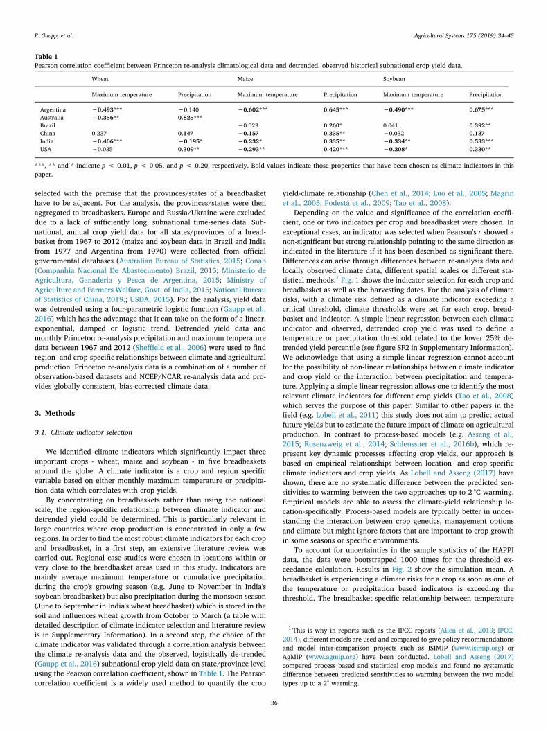
Table 1Pearson correlation coefficient between Princeton re-analysis climatological data and detrended, observed historical subnational crop yield data.

Wheat Maize Soybean

Maximum temperature Precipitation Maximum temperature Precipitation Maximum temperature Precipitation

Argentina −0.493*** −0.140 −0.602*** 0.645*** −0.490*** 0.675***Australia −0.356** 0.825***Brazil −0.023 0.260* 0.041 0.392**China 0.237 0.147 −0.157 0.335** −0.032 0.137India −0.406*** −0.195* −0.232* 0.335** −0.334** 0.533***USA −0.035 0.309** −0.293** 0.420*** −0.208* 0.330**

***, ** and * indicate p < 0.01, p < 0.05, and p < 0.20, respectively. Bold values indicate those properties that have been chosen as climate indicators in thispaper.

1 This is why in reports such as the IPCC reports (Allen et al., 2019; IPCC,2014), different models are used and compared to give policy recommendationsand model inter-comparison projects such as ISIMIP (www.isimip.org) orAgMIP (www.agmip.org) have been conducted. Lobell and Asseng (2017)compared process based and statistical crop models and found no systematicdifference between predicted sensitivities to warming between the two modeltypes up to a 2° warming.

F. Gaupp, et al. Agricultural Systems 175 (2019) 34–45

36

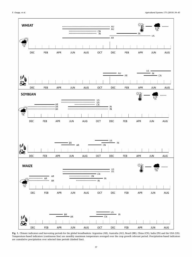
Fig. 1. Climate indicators and harvesting periods for the global breadbaskets: Argentina (AR), Australia (AU), Brazil (BR), China (CN), India (IN) and the USA (US).Temperature-based indicators (continuous line) are monthly maximum temperature averaged over the crop growth relevant period. Precipitation-based indicatorsare cumulative precipitation over selected time periods (dashed line).

F. Gaupp, et al. Agricultural Systems 175 (2019) 34–45

37

and precipitation is accounted for through the copula correlationstructure explained in Section 3.3.

3.2. Bias-correction

In order to quantify the likelihood of threshold exceedance of dif-ferent climate indicators, the HadAM3P model output has to be com-parable to the observed historical climate used for setting thesethresholds. Therefore, both historical and future experiment resultswere calibrated using a simple bias-correction method (Hawkins et al.,2013; Ho, 2010) which corrects mean and variability biases of theclimate indicators distributions using the Princeton re-analysis data(Sheffield et al., 2006) as calibration dataset:

= +I t O I t I( ) ( ( ) )BC REFO REF

I REFREF REF

,

, (1)

= +I t O I t I( ) ( ( ) )FUT BC REFO REF

I REFFUT REF,

,

, (2)

IBC denotes the HAPPI HadAM3P bias-corrected climate indicator,OREF and IREF the observational Princeton dataset and HAPPI HadAM3Phistorical raw climate indicators and IFUT represents the 1.5 or 2 °C rawclimate indicator. This method has the advantage of being simple tocalculate and being independent of the shape of the climate variabledistribution (Hawkins et al., 2013). It is used widely in agriculturalmodelling (Navarro-Racines et al., 2016). Although for precipitationusually a more complicated calibration method has to be applied as itcannot take negative values, in this case it was possible as we use ag-gregated precipitation values which never reach zero. HadAM3P gen-erally overestimated temperature compared to the Princeton datasetwith HadAM3P maximum temperature being between 7 and 57%higher than Princeton in all breadbaskets. Precipitation is

underestimated in the maize and soybean breadbaskets by between 2and 30%. Precipitation for wheat, which has a different growing season,is both higher and lower than the reference dataset (between 40%lower in Australia and 37% higher in the US breadbasket).

3.3. Regular vine copulas

In this study, climate indicators based on historical Princeton re-analysis data were used to estimate the spatial dependence structurebetween the five breadbaskets to avoid biases in inter-regional corre-lation in the HadAM3P climate model. As the dependence structure ofthe HAdAM3P climate indicators in the different breadbaskets did notchange between historical and warming scenarios, we kept the histor-ical dependence structure constant in the 1.5 and 2 °C scenarios.Changes in simultaneous climate risks between scenarios occur due tochanges in mean and variance of the underlying marginal distributionsof the climate indicators based on HadAM3P data.

In order to estimate risks of multiple breadbasket failure owing tojoint climate extremes in major crop production areas,2 the spatialdependence structure of the global breadbasket's climate indicators wasmodelled using regular vine (RVine) copulas (Aas et al., 2009; Dißmannet al., 2013; Kurowicka and Cooke, 2006). RVines are a flexible class ofmultivariate copulas which are able to model complex dependencies inlarger dimensions. They are based on Sklar's theorem (Sklar, 1959)which states that any multivariate distribution F can be written as

… = …F x x C F x F x( , , ) [ ( ), , ( )]n n n1 1 1 (3)

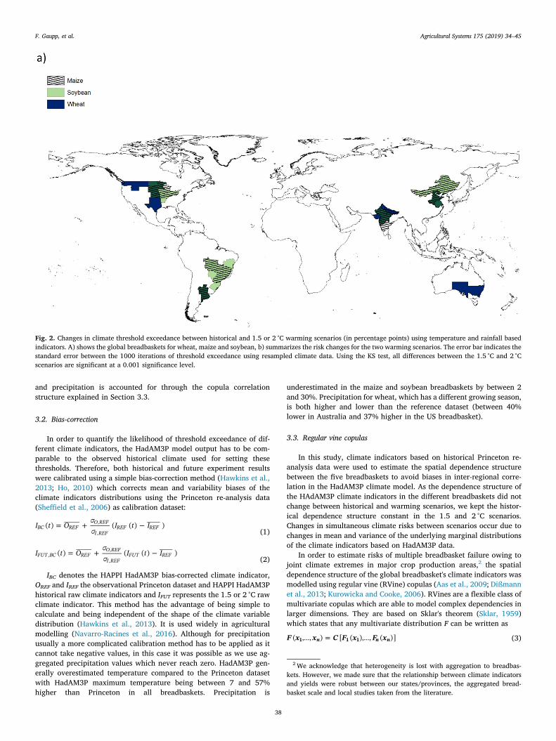
Fig. 2. Changes in climate threshold exceedance between historical and 1.5 or 2 °C warming scenarios (in percentage points) using temperature and rainfall basedindicators. A) shows the global breadbaskets for wheat, maize and soybean, b) summarizes the risk changes for the two warming scenarios. The error bar indicates thestandard error between the 1000 iterations of threshold exceedance using resampled climate data. Using the KS test, all differences between the 1.5 °C and 2 °Cscenarios are significant at a 0.001 significance level.

2 We acknowledge that heterogeneity is lost with aggregation to breadbas-kets. However, we made sure that the relationship between climate indicatorsand yields were robust between our states/provinces, the aggregated bread-basket scale and local studies taken from the literature.

F. Gaupp, et al. Agricultural Systems 175 (2019) 34–45

38

Fig. 2. (continued)

F. Gaupp, et al. Agricultural Systems 175 (2019) 34–45

39

with marginal probability distributions F1(x1), …, Fn(xn) and C denotingan n-dimensional copula, a multivariate distribution on the unit hy-percube [0,1]2 with uniform marginal distributions. Vine copulas areconstructed using conditional and unconditional bivariate pair-copulasfrom a set of copula families with distinct dependence structures (Aaset al., 2009; Joe, 1997). A set of linked RVine trees describes the fac-torisation of the copula's multivariate density function (Bedford andCooke, 2002). An n-dimensional RVine model consists of (n-1) treesincluding Ni nodes and Ei-1 edges which join the nodes. The treestructure is built according to the proximity condition which means thatif an edge connects two nodes in tree j+ 1, the corresponding edges intree j share a node (Bedford and Cooke, 2002). The first tree consist ofn-1 pairs of variables with directly modelled distributions. The secondtree identifies n-2 variable pairs with a distribution modelled by a pair-copula conditional on a single variable which is determined in thesecond tree. Proceeding in this way, the last tree consist of a single pairof variables with a distribution conditional on all remaining variables,defined by a last pair-copula (Dißmann et al., 2013). The RVine treestructure, the pair-copula families and the copula parameters are esti-mated in an automated way starting with the first tree. The tree is se-lected using a maximum spanning tree algorithm and Kendall's tau asedge weights. The best fitting pair-copula family is chosen using theAkaike Information Criterion (Akaike, 1973) and copula parameters areestimated using Maximum Likelihood Estimation (MLE). In this studywe chose from six different copula families representing different typesof tail dependencies to capture the exact patterns of dependence be-tween the different climate indicators in the crop breadbaskets: Gaus-sian, Clayton, Student-t, Gumbel, Joe and Frank copulas (Nelsen, 2007).

3.4. Impact on agricultural production

We analyse events where the climatic conditions in all five bread-baskets are associated with losses in agricultural yields. We identify a‘breadbasket failure’ event as being when the climatic conditions are atleast as severe as those conditions associated with the 25 percentile ofthe logistically detrended yields (with detrended yields as residuals ofthe non-linear logistic regression with a residual mean equal to zero).The crop production loss for an event of this severity is the 25 percentileof the logistically detrended yield multiplied with the 2012 harvestedarea. Given that we identify climatic events that are at least as severe asthis condition, our estimated loss is the lower bound on the loss, i.e. theminimum expected loss. Minimum expected losses are then defined asthe sum of crop losses in all five breadbaskets multiplied with the jointprobability that climate thresholds are exceeded in all regions si-multaneous as shown in Eq. (4):

Minimum expected losses y area p25(| | )i

BB

i i 2012 5,(4)

with

=

=

p

P Clim t Clim t Clim t Clim t Clim t

C F t F t F t F t F t( , , , , )[ ( ), ( ), ( ), ( ), ( )]

Clim Clim Clim Clim Clim

clim clim clim clim clim

5

1 2 3 4 5

1 2 3 4 5

1 2 3 4 5

1 2 3 4 5.

with y25i as the 25 percentile of logistically detrended yields in thebreadbasket i which was used to define climate thresholds and whichindicates a minimum yield loss, areai,2012 as the 2012 harvested area inbreadbasket i and with p5 as the probability of all five breadbasketsexceeding the climate thresholds in the same year. Climi denotes thetemperature or precipitation-based climate indicator, associated withthe 25 percentile of the detrended yields. In case that a breadbasket hastwo indicators for a crop, the exceedance of at least one of the climatethresholds tclimi

is counted as threshold exceedance in the breadbasket.C denotes the copula.

4. Results

4.1. Changes in climate risks to agriculture under 1.5 and 2 °C globalwarming

The change of climate risks to major crops in the global breadbas-kets were examined for each region and crop separately comparinghistorical risks with risks associated with a 1.5 and 2 °C global warming,shown in Fig. 2. As expected from an increase of global mean tem-perature, temperature based climate risks are increasing, but to dif-ferent extents depending on the region. Precipitation signals associatedwith 1.5 and 2 °C warming are less clear. While precipitation basedclimate risks in the US and Brazil increase in both scenarios for thesummer crops maize and soybean, precipitation in Argentina does notsignificantly change. Risks in China and India decrease due to an in-crease in monsoon precipitation. For wheat, precipitation-based climaterisks only increase in Australia.

The decrease of precipitation-based climate risks to wheat in the USand China, and the increase in the Australian breadbaskets for bothwarming scenarios mostly coincide with findings of a previous study(Gaupp et al., 2016) which examined climate risk trends in the past. InIndia and China, wheat is indirectly impacted by the summer monsoonrainfall which provides stored soil moisture for the “rabi” wheat crop.Although precipitation between June and September in the Chinesebreadbasket showed a decrease in the recent past, in a 1.5 and 2 °Cwarmer world precipitation during monsoon months in the Chinesebreadbasket is projected to increase. This coincides with (Lv et al.,2013) who project a decrease in precipitation in China during the wheatgrowing season between the 2000s and 2030s and a consistent pre-cipitation increase from the 2030s to the 2070s. In India, rainfall duringsummer monsoon months (June to September) showed a decreasingdecadal trend in the recent past (Guhathakurta et al., 2015) which wasreflected in an increasing climate risk for wheat in India in the past(Gaupp et al., in review). In the future, however, monsoon precipitationis projected to increase under all RCP scenarios in CMIP5 projections(Jayasankar et al., 2015; Menon et al., 2013) which coincides withdecreasing precipitation climate risks to wheat in the Indian bread-basket found in this study. However, precipitation-based risks in Indiaand China might be underestimated in this study because of the HAPPIexperiment structure which has fixed SSTs driving the model, ratherthan a fully couple ocean simulation. This often leads to variability inland-ocean driven cycles not changing much and thereby to an under-estimation of precipitation variability during the monsoon months.CMIP5 models project both increasing and decreasing standard devia-tions of monsoon precipitation in India for RCP 2.6 and 4.5. In Aus-tralia, precipitation in the wheat growing season is projected to de-crease following different CMIP5 models under RCP4.5 (Ummenhoferet al., 2015) which our study confirms through increased precipitation-based climate risks. Temperature risks are increasing in all temperaturesensitive breadbaskets with stronger increases in India and Australiathan in Argentina. Our estimates of climate risks to wheat productioncoincide with results of crop model experiments in other studies. Assenget al. (2015) compared results of 30 wheat crop simulation models in 30main wheat producing locations without water stress, focussing only onthe effect of temperature. All models showed yield losses at a 2 °Cwarming, which coincides with our temperature-based climate riskincreases in India, Australia and Argentina. Rosenzweig et al. (2018)and Ruane et al. (2018) used HAPPI climate data and other climatemodel experiments from CMIP5 to compare climate impacts on cropsunder a 1.5 °C and 2 °C warming using process-based crop models. Theyfound wheat yield losses smaller than 5% in the North American GreatPlains, but larger losses in Australia and Argentina under 1.5 °Cwarming. In India and China the models showed yield increases in a1.5 °C world. Challinor et al. (2014) came to similar conclusions in ameta-analysis of crop yield under climate change. He found no changesin wheat yields under a 1.5 °C warming in tropical regions but a slight

F. Gaupp, et al. Agricultural Systems 175 (2019) 34–45

40

Fig. 3. Risks of multiple breadbasket failure under 1.5 and 2 °C warming. Error bars reflect the sampling error as well as the copula simulation error which wasdetermined in 1000 iterations.

F. Gaupp, et al. Agricultural Systems 175 (2019) 34–45

41

decrease under 2 °C. In temperate regions, such as the US, China orArgentina, wheat yields are projected to decrease for both warminglevels, when adaptation strategies such as irrigation, planting times ofcrop varieties are not considered.

For soybean, precipitation-based climate risks in South Americaincrease in Brazil but do not change notably in Argentina. This coin-cides with findings from other CMIP5 studies (Barros et al., 2015; IPCC,2014). In the US, CMIP5 models show a small, not significant increasein annual precipitation (IPCC, 2014)) which can be seen in HadAM3P aswell. Precipitation during the soybean growing season, on the otherhand, is projected to decrease in both 1.5 and 2 °C scenarios whichresults in higher climate risks. In China and India, soybean growingseasons are directly aligned with the summer monsoon. Hence, pre-cipitation-based soybean climate risks decrease due to the above dis-cussed increase in monsoon precipitation. Temperature based risks, onthe other hand, increase significantly in the US, Argentina and India.Those temperature and precipitation changes translated into yieldchanges in several crop model experiments for rainfed and irrigatedsoybean. The models show slight yield decreases over the interior ofNorthern America but small increases towards the eastern US in a 1.5 °Cscenario for rainfed soybean. In Brazil and Argentina, soybean showsboth increases and decreases under a 1.5 °C warming and in the Indianbreadbasket, soybean yields are projected to increase. In China, yieldsare projected to increase in the North, but decrease in the South. Modelsfor irrigated crop that also include CO2 benefits, yields are projected toincrease (Ruane et al., 2018). Under a 2 °C warming, GCMs revealedyield increases when CO2 effects were considered as they largelyovercome increased temperature risks (Ruane et al., 2018; Schleussneret al., 2016a).

For maize, climate risks show very similar patterns to soybean as thetwo summer crops have similar growing seasons and indicators.Additional to the soybean climate indicators, maize in the Chinesebreadbasket is sensitive to temperature. Owing to those local pre-cipitation changes and temperature rise, global crop models (GCMs)have shown declines in maize yields in all five breadbaskets in both a1.5 and 2 °C warmer world (Ruane et al., 2018; Schleussner et al.,2016a). In contrast to soybean, maize is not able to capture the samelevel of CO2 benefits and hence yields decrease further under in a 2 °Cworld. Those finding coincide with results of the meta-study byChallinor et al. (2014).

One of the major concerns in studies of the difference between a 1.5and 2 °C global warming is the significance of the difference betweenthe temperature increments (James et al., 2017). The difference be-tween climate risks for 1.5 and 2 °C in this study was tested with thestudent two-sample Kolmogorov-Smirnov (KS) test which tests the nullhypothesis that both distributions of resampled threshold exceedanceare drawn from the same distribution. Results showed significant dif-ferences for all indicators and crops at the 0.001 significance levelbetween the two warming levels. The KS test allows for robust state-ments about the difference between climate risks under 1.5 and 2 °Cwarming even if there is an overlap of uncertainty bands (Schleussneret al., 2016a). Error bars are small compared to the absolute change inclimate threshold exceedance with the exception of precipitation risksin Argentina for soybean and maize. Fig. 2 also compares the differencein changes from historical climate for both global mean temperatureincreases. Across all three crops, we found stronger signals for tem-perature based risks than for precipitation based risks which showsmaller, both positive and negative signals. Additionally, the differencebetween the 1.5 and 2 °C warming is more pronounced in temperaturebased indicators with the largest difference in the Indian soybeanbreadbasket (26% points). The difference in precipitation risk changesbetween the two warming scenarios lies between 0 and 6% points.What stands out is the difference between 1.5 and 2 °C for precipitationrisks in Brazil. In contrast to other climate indicators, precipitationbetween December and February and March in Brazil shows a sig-nificantly stronger difference from historical data to 1.5 °C than to 2 °C.

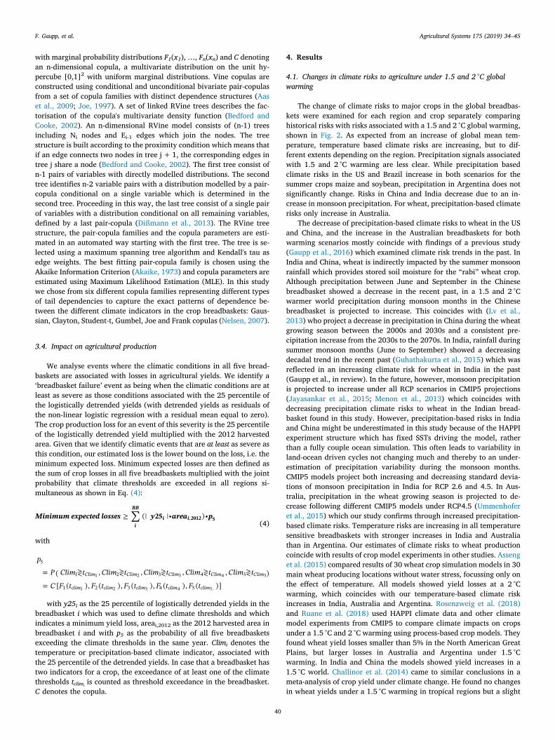
4.2. Increasing risks of multiple breadbasket failure

Having analysed individual changes of climate risks in the globalwheat, soybean and maize breadbaskets for 1.5 and 2 °C enables us tocalculate joint climate risks on a global scale. Fig. 3 shows the largestincrease in risks of simultaneous crop failure (resulting from climateexceeding a crop- and region-specific threshold) in the global bread-baskets for maize, followed by soybean and wheat. For all three cropsthe likelihoods that none or just one of the breadbaskets experiencesclimate risks decreases to (nearly) zero. For wheat and soybean, thelikelihoods of breadbaskets experiencing detrimental climate changeincreases significantly from the historical scenario to 1.5 °C and evenmore assuming 2 °C warming. The figure can be interpreted as a dis-crete probability distribution with the sum of all breadbasket thresholdexceedances adding up to 1. The shape of the distribution stays roughlythe same across warming scenarios with higher probabilities that partsof the breadbaskets exceed the thresholds and smaller likelihoods in theextremes. While the historical baseline climate still shows the prob-ability for zero simultaneous climate risks, for higher temperaturescenarios these likelihoods disappear. The average threshold ex-ceedance increases significantly (measured using the KS-test), more forsoybean than for wheat. For maize, likelihoods of simultaneous climaterisks increase strongly. Under the 2 °C scenario the likelihood of all fivebreadbaskets suffering detrimental climate is the highest. For wheat,which shows the smallest simultaneous climate risks, the return periodfor all five breadbaskets exceeding their climate thresholds decreasesfrom 43 years (or 0.023 annual probability under historical conditionsto 21 years (0.047) in a 1.5 °C scenario and further down to around15 years (0.066) under 2 °C. Soybean has a return period of simulta-neous climate risks in all breadbaskets of around 20 years (0.049 todaywhich decreases to 9 (0.116) and 7 years (0.143 in a 1.5 and 2 °Cwarmer world respectively. Maize risks are highest in our study with aninitial return period of 16 years (0.061), decreasing to<3 (0.39)and< 2 years (0.538) under future global warming. In general, one cansay that whilst the differences in yield at 1.5 vs 2 °C are significant theyare not as large as the difference between 1.5 and historical. Risk ofsimultaneous crop failure, however, do increase disproportionatelybetween 1.5 and 2° and this is important because correlated risks leadto disproportionately high impacts.

To illustrate the effects of simultaneous climate risks in a 1.5 and a2 °C warmer world, we estimated the impacts on agricultural produc-tion. Simultaneous crop failure in all breadbaskets, defined as the 25percentile of detrended yield, would add up to at least 9.86 million tonsof soybean losses, 19.75 million tons of maize losses and 8.59 milliontons of wheat losses assuming 2012 agricultural area. Historical ex-amples of global crop production shocks include 7.2 million tons soy-bean losses in 1988/99 and 55.9 million tons maize losses in 1988which were mostly caused by low rainfall and high temperatures duringsummer growing season in the US (Bailey and Benton, 2015). Historicalglobal wheat production shocks include 36.6 million tons wheat lossesin 2003 mostly caused by heat waves and drought in spring in Europeand Russia but also by reduced acreage due to drought or winterkill inEurope, India and China (Bailey and Benton, 2015). Maize and wheatlosses in this study are lower than in historical cases as our breadbasketsonly account for 38% and 52% of global production respectively.Soybean in this study accounts for 80% of global production. Com-bining absolute losses with likelihoods of simultaneous climate risks,we calculated expected crop losses following Eq. (4). For all three crops,expected crop losses are significantly higher under the 2 °C than underthe 1.5 °C scenario. Under a scenario of 2 °C mean global warming,expected wheat, maize and soybean losses are projected to be 161,000,2753 000 and 265,000 t higher than if global temperature increases arelimited to 1.5 °C. This equals total annual maize production in Uganda,the world's 33rd largest maize producer in 2012. The difference ofwheat losses is larger than Bolivia's annual total production in 2012(145,000 t) and the increase of expected soybean losses is comparable

F. Gaupp, et al. Agricultural Systems 175 (2019) 34–45

42

to Mexico's annual production (248,000 t), the world's 20th biggestsoybean producer (FAO, 2015).

To test for the influence of inter-dependence between the climateindicators in the different breadbaskets on the results of this analysis,we excluded the correlations between them. We assumed independencebetween the breadbaskets, but still accounted for the negative corre-lation between temperature and precipitation indices within onebreadbasket. Supplementary Figure SF3 illustrates the difference be-tween independence and correlation. Between the three crops, noconsistent pattern was found between dependent and independentcases. The only crop that shows significant differences is soybean withsmaller likelihoods in the extremes when dependence is excluded. Thismeans that the likelihood of all five soybean breadbaskets experiencingdetrimental climate in one year is underestimated if correlations be-tween the breadbaskets are not considered in a risk analysis. Expressedin expected production losses, the losses are up lo 190,000 t higher inthe dependent case which is more than what the 22nd largest soybeanproducer harvests annually (FAO, 2015). For wheat and maize, thedifference between the dependencies was mostly not significant.

5. Discussion

Our results illustrate future climate conditions under two warmingscenarios in the global breadbaskets and investigate simultaneous cli-mate risks affecting three major crops. The study focused explicitly onthe climate impact on crop yields. The effects of other factors such assoil quality, land management, land use or technology were held con-stant under future warming scenarios. Therefore, our estimates of cropproduction losses have to be interpreted with care. By not explicitlyincluding CO2 concentrations, for instance, the CO2 fertilizer effectwhich increases productivity in wheat and soybean and to a certainextent in maize (Schleussner et al., 2016a) was not taken into account.The effects of climatic change on plant phenology were not considered.In China, for instance, the flowering date of wheat is projected to ad-vance owing to increased temperatures and the gain-filling period willshorten which might further reduce yields (Lv et al., 2013). By holdingharvested area constant at 2012 levels, shifts in land use and croppedarea in response to projected climatic changes (Nelson et al., 2014;Schmitz et al., 2014) were not considered. Owing to a lack of subna-tional historic time series of irrigated crop yields, irrigation was notspecifically taken into account in setting climate risk thresholds. Thiswas acceptable in this study as, even without considering irrigation, thecorrelation coefficients between observed, detrended yields and climateindicators were mostly significant. A large share of the regions in thisstudy are completely rain-fed. In other regions such as India or the US,irrigated crops still show correlations with rainfall (Pathak andWassmann, 2009) or no significant difference to rain-fed crops at all(Zhang et al., 2015). Results of the analysis of simultaneous climaterisks may vary depending on the climate indicator selection. The two-step approach of pre-selecting potential indicators in a literature reviewand verification through the correlation analysis with re-analysis cli-mate data and observed historical yield data represents a robust way ofindicator selection. However, including different climate variables suchas number of days above a crop dependent heat threshold (Schlenkerand Roberts, 2009; Tack et al., 2015; Zhang et al., 2015) or dry spelllength (Hernandez et al., 2015; Ramteke et al., 2015; Schleussner et al.,2016a) might lead to different results. So far, the HAPPI project onlyprovides monthly data which limited the climate variable choice. Inorder to reduce uncertainties, we bootstrapped the climate indicatorsand repeatedly simulated the copula models. However, results from 1.5and 2 °C warming scenarios vary between different GCMs (Schleussneret al., 2016a). A comparison with additional climate models from theHAPPI project will further improve the robustness of the results.

6. Conclusion

This study found disproportionally increasing future risks of si-multaneous crop failure in the global wheat, maize and soybeanbreadbaskets in a 1.5 and 2 °C warmer world using results of theHadAM3P atmospheric model as part of the HAPPI experiment.Increases in temperature-based climate risks were found to be strongerthan precipitation-based risks which showed different signals de-pending on crop and region. Using the copula methodology, it waspossible to capture dependence structures between regions and to cal-culate joint climate risks in the major crop producing areas.Additionally, the copula analysis accounted for the region-specific re-lationships between temperature and precipitation. Strongest increasesin simultaneous climate risks were found for maize where return per-iods of simultaneous crop failure decrease from 16 years in the pastto< 3 and<2 years under 1.5 and 2 °C warming. In percentage terms,the largest increase of simultaneous climate threshold exceedance in allfive breadbaskets between the two warming scenarios was found forwheat (40%), followed by maize (35%) and soybean (23%). Looking atthe impacts on crop production, the study showed that limiting globalwarming to 1.5 °C would avoid production losses of up to 2753 million(161,000, 265,000) tonnes maize (wheat, soybean) in the main pro-duction regions.

Our study represents an important first step in the analysis of dif-ferential temperature increases of 1.5 and 2 °C and their impacts onagricultural production. Compared to climate studies which often focuson average annual values, this study focused on crop growth periodswhich may show opposite signals to annual means – as shown here forsoybean in the US - and therefore added valuable information to ex-isting studies.

Results are based on HadAM3P, the first model in the HAPPI ex-periment set up. Including outputs from additional climate models willgive more robust information on future climate risks. Additionally,further analysis of the ability of climate models to accurately modelspatial dependence between regions is needed. This study used histor-ical dependence to avoid biases in spatial correlation and kept depen-dence constant under future scenarios. Some literature, however, sug-gests that teleconnection patterns might change, i.e. owing to changesin El Niño Southern Oscillation (ENSO) (Cai et al., 2014; Power et al.,2013), which could then alter the spatial climate dependence structurein the breadbaskets. Future work (under preparation) will look intoclimate risks under different ENSO phases.

This paper provides insights into risks of multiple breadbasketfailure under 1.5 and 2 °C warming which can contribute to currentclimate policy discussions and potentially provides useful informationfor the Intergovernmental Panel on Climate Change (IPCC) SpecialReport on the impact of 1.5 °C global warming commissioned by theUN-FCCC after the Paris Agreement.

Acknowledgements

This research was financially supported by the project ECOCEP,funded by the People Programme (Marie Curie Actions) of the EuropeanUnion’s Seventh Framework Programme FP7-PEOPLE-2013-IRSES,Grant Agreement No 609642. It was also supported by IIASA and itsNational Member Organizations in Africa, the Americas, Asia, andEurope.

Appendix A. Supplementary data

Supplementary data to this article can be found online at https://doi.org/10.1016/j.agsy.2019.05.010.

F. Gaupp, et al. Agricultural Systems 175 (2019) 34–45

43

References

Aas, K., Czado, C., Frigessi, A., Bakken, H., 2009. Pair-copula constructions of multipledependence. Insur. Math. Econ. 44, 182–198. https://doi.org/10.1016/j.insmatheco.2007.02.001.

Akaike, H., 1973. Information theory and an extension of the maximum likelihoodprinciple. In: Petran, B.N., Csáki, F. (Eds.), International Symposium on InformationTheory, Second Edition. Akadémiai Kiadi, Budapest, Hungary, pp. 267–281.

Allen, M., Antwi-Agyei, P., Aragon-Durand, F., Babiker, M., Bertoldi, P., Bind, M., Brown,S., Buckeridge, M., Camilloni, I., Cartwright, A., 2019. Technical Summary: GlobalWarming of 1.5° C. An IPCC Special Report on the Impacts of Global Warming of 1.5°C above Pre-Industrial Levels and Related Global Greenhouse Gas EmissionPathways. (in the context of strengthening the global response to the threat of cli-mate change, sustainable development, and efforts to eradicate poverty).

Anderson, D.P., 2004. Boinc: A system for public-resource computing and storage. In:Grid Computing, 2004, Proceedings, Fifth IEEE/ACM International Workshop onIEEE, pp. 4–10.

Asseng, S., Ewert, F., Martre, P., Rötter, R.P., Lobell, D.B., Cammarano, D., Kimball, B.A.,Ottman, M.J., Wall, G.W., White, J.W., Reynolds, M.P., Alderman, P.D., Prasad,P.V.V., Aggarwal, P.K., Anothai, J., Basso, B., Biernath, C., Challinor, A.J., De Sanctis,G., Doltra, J., Fereres, E., Garcia-Vila, M., Gayler, S., Hoogenboom, G., Hunt, L.A.,Izaurralde, R.C., Jabloun, M., Jones, C.D., Kersebaum, K.C., Koehler, A.-K., Müller, C.,Naresh Kumar, S., Nendel, C., O'Leary, G., Olesen, J.E., Palosuo, T., Priesack, E., EyshiRezaei, E., Ruane, A.C., Semenov, M.A., Shcherbak, I., Stöckle, C., Stratonovitch, P.,Streck, T., Supit, I., Tao, F., Thorburn, P.J., Waha, K., Wang, E., Wallach, D., Wolf, J.,Zhao, Z., Zhu, Y., 2015. Rising temperatures reduce global wheat production. Nat.Clim. Chang. 5, 143–147. https://doi.org/10.1038/nclimate2470.

Australian Bureau of Statistics, 2015. Historical Selected Agriculture Commodities. URL.http://www.abs.gov.au/.

Bailey, R., Benton, T., 2015. Extreme Weather and Resilience of the Global Food System.Final Project Report from the UK-US Taskforce on Extreme Weather and Global FoodSystem Resilience. The Global Food Security Programme, UK.

Barros, V.R., Boninsegna, J.A., Camilloni, I.A., Chidiak, M., Magrín, G.O., Rusticucci, M.,2015. Climate change in Argentina: trends, projections, impacts and adaptation:climate change in Argentina. Wiley Interdiscip. Rev. Clim. Chang. 6, 151–169.https://doi.org/10.1002/wcc.316.

Bedford, T., Cooke, R.M., 2002. Vines: a new graphical model for dependent randomvariables. Ann. Stat. 1031–1068.

Bren d'Amour, C., Wenz, L., Kalkuhl, M., Christoph Steckel, J., Creutzig, F., 2016.Teleconnected food supply shocks. Environ. Res. Lett. 11, 035007. https://doi.org/10.1088/1748-9326/11/3/035007.

Cai, W., Borlace, S., Lengaigne, M., Van Rensch, P., Collins, M., Vecchi, G., Timmermann,A., Santoso, A., McPhaden, M.J., Wu, L., others, 2014. Increasing frequency of ex-treme El Niño events due to greenhouse warming. Nat. Clim. Change 4, 111–116.

Challinor, A.J., Watson, J., Lobell, D.B., Howden, S.M., Smith, D.R., Chhetri, N., 2014. Ameta-analysis of crop yield under climate change and adaptation. Nat. Clim. Chang.4, 287.

Chen, H., Wang, J., Huang, J., 2014. Policy support, social capital, and farmers' adap-tation to drought in China. Glob. Environ. Change 24, 193–202. https://doi.org/10.1016/j.gloenvcha.2013.11.010.

Conab (Companhia Nacional De Abastecimento) Brazil, 2015. Séries históricas. URL.http://www.conab.gov.br.

Dißmann, J., Brechmann, E.C., Czado, C., Kurowicka, D., 2013. Selecting and estimatingregular vine copulae and application to financial returns. Comput. Stat. Data Anal.59, 52–69. https://doi.org/10.1016/j.csda.2012.08.010.

FAO, 2014. Strengthening the Enabling Environment for Food Security and Nutrition: TheState of Food Insecurity in the World. FAO, Rome.

FAO, 2015. Statistical Database.Field, C.B., IPCC (Eds.), 2012. Managing the Risks of Extreme Events and Disasters to

Advance Climate Change Adaption: Special Report of the Intergovernmental Panel onClimate Change. Cambridge University Press, New York, NY.

Fischer, E.M., Knutti, R., 2015. Anthropogenic contribution to global occurrence ofheavy-precipitation and high-temperature extremes. Nat. Clim. Chang. 5, 560–564.https://doi.org/10.1038/nclimate2617.

Fraser, E.D.G., Simelton, E., Termansen, M., Gosling, S.N., South, A., 2013. “Vulnerabilityhotspots”: integrating socio-economic and hydrological models to identify wherecereal production may decline in the future due to climate change induced drought.Agric. For. Meteorol. 170, 195–205. https://doi.org/10.1016/j.agrformet.2012.04.008.

Gaupp, F., Pflug, G., Hochrainer-Stigler, S., Hall, J., Dadson, S., 2016. Dependency of cropproduction between global breadbaskets: a copula approach for the assessment ofglobal and regional risk pools. Risk Anal. 37 (11), 2212–2228.

Gordon, C., Cooper, C., Senior, C.A., Banks, H., Gregory, J.M., Johns, T.C., Mitchell, J.F.,Wood, R.A., 2000. The simulation of SST, sea ice extents and ocean heat transports ina version of the Hadley Centre coupled model without flux adjustments. Clim. Dyn.16, 147–168.

Guhathakurta, P., Rajeevan, M., Sikka, D.R., Tyagi, A., 2015. Observed changes insouthwest monsoon rainfall over India during 1901-2011: TREND IN SOUTHWESTMONSOON RAINFALL OVER INDIA. Int. J. Climatol. 35, 1881–1898. https://doi.org/10.1002/joc.4095.

Hawkins, E., Osborne, T.M., Ho, C.K., Challinor, A.J., 2013. Calibration and bias cor-rection of climate projections for crop modelling: an idealised case study over Europe.Agric. For. Meteorol. 170, 19–31. https://doi.org/10.1016/j.agrformet.2012.04.007.

Hernandez, V., Moron, V., Riglos, F.F., Muzi, E., 2015. Confronting farmers' perceptionsof climatic vulnerability with observed relationships between yields and climate

variability in Central Argentina. Weather Clim. Soc. 7, 39–59.Ho, C.K., 2010. Projecting Extreme Heat-Related Mortality in Europe under Climate

Change.IPCC, 2014. Climate Change 2014–Impacts, Adaptation and Vulnerability: Regional

Aspects. Contribution of Working Group II to the Fifth Assessment Report of theIntergovernmental Panel on Climate Change. Cambridge University Press,Cambridge, United Kingdom and New York, NY, USA.

James, R., Washington, R., Schleussner, C.-F., Rogelj, J., Conway, D., 2017.Characterizing half-a-degree difference: a review of methods for identifying regionalclimate responses to global warming targets: characterizing half-a-degree difference.Wiley Interdiscip. Rev. Clim. Chang. e457. https://doi.org/10.1002/wcc.457.

Jayasankar, C.B., Surendran, S., Rajendran, K., 2015. Robust signals of future projectionsof Indian summer monsoon rainfall by IPCC AR5 climate models: role of seasonalcycle and interannual variability: FUTURE PROJECTIONS OF ISMR. Geophys. Res.Lett. 42, 3513–3520. https://doi.org/10.1002/2015GL063659.

Joe, H., 1997. Multivariate Models and Multivariate Dependence Concepts. CRC Press.Kurowicka, D., Cooke, R.M., 2006. Uncertainty Analysis with High Dimensional

Dependence Modelling. John Wiley & Sons.Lobell, D.B., Asseng, S., 2017. Comparing estimates of climate change impacts from

process-based and statistical crop models. Environ. Res. Lett. 12, 015001.Lobell, D.B., Schlenker, W., Costa-Roberts, J., 2011. Climate trends and global crop

production since 1980. Science 333, 616–620.Lunt, T., Jones, A.W., Mulhern, W.S., Lezaks, D.P.M., Jahn, M.M., 2016. Vulnerabilities to

agricultural production shocks: an extreme, plausible scenario for assessment of riskfor the insurance sector. Clim. Risk Manag. 13, 1–9. https://doi.org/10.1016/j.crm.2016.05.001.

Luo, Q., Bellotti, W., Williams, M., Bryan, B., 2005. Potential impact of climate change onwheat yield in South Australia. Agric. For. Meteorol. 132, 273–285. https://doi.org/10.1016/j.agrformet.2005.08.003.

Lv, Z., Liu, X., Cao, W., Zhu, Y., 2013. Climate change impacts on regional winter wheatproduction in main wheat production regions of China. Agric. For. Meteorol. 171,234–248.

Magrin, G.O., Travasso, M.I., Rodríguez, G.R., 2005. Changes in climate and crop pro-duction during the 20th century in Argentina. Clim. Chang. 72, 229–249.

Massey, N., Jones, R., Otto, F.E.L., Aina, T., Wilson, S., Murphy, J.M., Hassell, D.,Yamazaki, Y.H., Allen, M.R., 2015. Weather@home-development and validation of avery large ensemble modelling system for probabilistic event attribution: weather@home. Q. J. R. Meteorol. Soc. 141, 1528–1545. https://doi.org/10.1002/qj.2455.

Maynard, T., 2015. Food System Shock: The Insurance Impacts of Acute Disruption toGlobal Food Supply. Lloyd’s of London, London, UK.

Menon, A., Levermann, A., Schewe, J., Lehmann, J., Frieler, K., 2013. Consistent increasein Indian monsoon rainfall and its variability across CMIP-5 models. Earth Syst. Dyn.4, 287–300. https://doi.org/10.5194/esd-4-287-2013.

Ministerio de Agricultura, Ganaderia y Pesca de Argentina, 2015. Statistical database.URL. http://www.siia.gov.ar/.

Ministry of Agriculture and Farmers Welfare, Govt. of India, 2015. Crop ProductionStatistics. URL. http://eands.dacnet.nic.in/.

Mitchell, D., AchutaRao, K., Allen, M., Bethke, I., Forster, P., Fuglestvedt, J., Gillett, N.,Haustein, K., Iverson, T., Massey, N., Schleussner, C.-F., Scinocca, J., Seland, Ø.,Shiogama, H., Shuckburgh, E., Sparrow, S., Stone, D., Wallom, D., Wehner, M.,Zaaboul, R., 2016a. Half a degree additional warming, projections, prognosis andimpacts (HAPPI): background and experimental design. Geosci. Model Dev. Discuss.1–17. https://doi.org/10.5194/gmd-2016-203.

Mitchell, D., James, R., Forster, P.M., Betts, R.A., Shiogama, H., Allen, M., 2016b.Realizing the impacts of a 1.5 [deg] C warmer world. Nat. Clim. Chang. 6 (8), 735.

National Bureau of Statistics of China, 2019. Regional data. URL. http://data.stats.gov.cn/.

Navarro-Racines, C.E., Tarapues-Montenegro, J.E., Ramírez-Villegas, J.A., 2016. Bias-Correction in the CCAFS-Climate Portal: A Description of Mehotodologies.

Nelsen, R.B., 2007. An Introduction to Copulas. Springer Science & Business Media.Nelson, G.C., Valin, H., Sands, R.D., Havlík, P., Ahammad, H., Deryng, D., Elliott, J.,

Fujimori, S., Hasegawa, T., Heyhoe, E., others, 2014. Climate change effects onagriculture: economic responses to biophysical shocks. Proc. Natl. Acad. Sci. 111,3274–3279.

Pathak, H., Wassmann, R., 2009. Quantitative evaluation of climatic variability and risksfor wheat yield in India. Clim. Chang. 93, 157–175. https://doi.org/10.1007/s10584-008-9463-4.

Podestá, G., Herrera, N., Veiga, H., Pujol, G., Skansi, M. de los M., Rovere, S., 2009.Towards a Regional Drought Monitoring and Warning System in Southern SouthAmerica: An Assessment of Various Drought Indices for Monitoring the 2007–2009Drought in the Argentine Pampas.

Pope, V., Stratton, R., 2002. The processes governing horizontal resolution sensitivity in aclimate model. Clim. Dyn. 19, 211–236. https://doi.org/10.1007/s00382-001-0222-8.

Pope, V.D., Gallani, M.L., Rowntree, P.R., Stratton, R.A., 2000. The impact of new phy-sical parameterizations in the Hadley Center coupled model without flux adjust-ments. Clim. Dyn. 17, 61–81.

Porter, J.R., Xie, L., Challinor, A.J., Cochrane, K., Howden, S.M., Iqbal, M.M., Lobell, D.B.,Travasso, M.I., 2014. Food security and food production systems. In: Climate Change2014: Impacts, Adaptation, and Vulnerability. In: Field, C.B., Barros, V.R., Dokken,D.J., Mach, K.J., Mastrandrea, M.D., Bilir, T.E. ... White, L.L. (Eds.), Part A: Globaland Sectoral Aspects. Contribution of Working Group II to the Fifth AssessmentReport of the Intergovernmental Panel on Climate Change. Cambridge UniversityPress, Cambridge, United Kingdom and New York, NY, USA.

Power, S., Delage, F., Chung, C., Kociuba, G., Keay, K., 2013. Robust twenty-first-centuryprojections of ElNino and related precipitation variability. Nature 502, 541–545.

F. Gaupp, et al. Agricultural Systems 175 (2019) 34–45

44

https://doi.org/10.1038/nature12580.Puma, M.J., Bose, S., Chon, S.Y., Cook, B.I., 2015. Assessing the evolving fragility of the

global food system. Environ. Res. Lett. 10, 024007. https://doi.org/10.1088/1748-9326/10/2/024007.

Ramteke, R., Gupta, G.K., Singh, D.V., 2015. Growth and yield responses of soybean toclimate change. Agric. Res. 4, 319–323. https://doi.org/10.1007/s40003-015-0167-5.

Rogelj, J., Knutti, R., 2016. Geosciences after Paris. Nat. Geosci. 9, 187–189.Rosenzweig, C., Elliott, J., Deryng, D., Ruane, A.C., Müller, C., Arneth, A., Boote, K.J.,

Folberth, C., Glotter, M., Khabarov, N., others, 2014. Assessing agricultural risks ofclimate change in the 21st century in a global gridded crop model intercomparison.Proc. Natl. Acad. Sci. 111, 3268–3273.

Rosenzweig, C., Ruane, A.C., Antle, J., Elliott, J., Ashfaq, M., Chatta, A.A., Ewert, F.,Folberth, C., Hathie, I., Havlik, P., Hoogenboom, G., Lotze-Campen, H., MacCarthy,D.S., Mason-D'Croz, D., Contreras, E.M., Mller, C., Perez-Dominguez, I., Phillips, M.,Porter, C., Raymundo, R.M., Sands, R.D., Schleussner, C.-F., Valdivia, R.O., Valin, H.,Wiebe, K., 2018. Coordinating AgMIP data and models across global and regionalscales for 1.5C and 2.0C assessments. Philos. Trans. R. Soc. Math. Phys. Eng. Sci. 376(2119), 20160455.

Ruane, A.C., Antle, J., Elliott, J., Folberth, C., Hoogenboom, G., Croz, D.M.-D., Müller, C.,Porter, C., Phillips, M.M., Raymundo, R.M., 2018. Biophysical and economic im-plications for agriculture of+ 1.5 and+ 2.0 C global warming using AgMIPCoordinated Global and Regional Assessments. Clim. Res. 76, 17–39.

Schaffnit-Chatterjee, C., Schneider, S., Peter, M., Mayer, T., 2010. Risk Management inAgriculture. (Dtsch. Bank Reseach Sept).

Schlenker, W., Roberts, M.J., 2009. Nonlinear temperature effects indicate severe da-mages to US crop yields under climate change. Proc. Natl. Acad. Sci. 106,15594–15598.

Schleussner, C.-F., Lissner, T.K., Fischer, E.M., Wohland, J., Perrette, M., Golly, A., Rogelj,J., Childers, K., Schewe, J., Frieler, K., Mengel, M., Hare, W., Schaeffer, M., 2016a.Differential climate impacts for policy-relevant limits to global warming: the case of1.5 &deg;C and 2 &deg;C. Earth Syst. Dyn. 7, 327–351. https://doi.org/10.5194/esd-7-327-2016.

Schleussner, C.-F., Rogelj, J., Schaeffer, M., Lissner, T., Licker, R., Fischer, E.M., Knutti,R., Levermann, A., Frieler, K., Hare, W., 2016b. Science and policy characteristics ofthe Paris agreement temperature goal. Nat. Clim. Chang. 6, 827–835. https://doi.

org/10.1038/nclimate3096.Schmitz, C., van Meijl, H., Kyle, P., Nelson, G.C., Fujimori, S., Gurgel, A., Havlik, P.,

Heyhoe, E., d'Croz, D.M., Popp, A., Sands, R., Tabeau, A., van der Mensbrugghe, D.,von Lampe, M., Wise, M., Blanc, E., Hasegawa, T., Kavallari, A., Valin, H., 2014.Land-use change trajectories up to 2050: insights from a global agro-economic modelcomparison. Agric. Econ. 45, 69–84. https://doi.org/10.1111/agec.12090.

Seneviratne, S.I., Donat, M.G., Pitman, A.J., Knutti, R., Wilby, R.L., 2016. Allowable CO2emissions based on regional and impact-related climate targets. Nature 529,477–483. https://doi.org/10.1038/nature16542.

Sheffield, J., Goteti, G., Wood, E.F., 2006. Development of a 50-year high-resolutionglobal dataset of meteorological forcings for land surface modeling. J. Clim. 19,3088–3111.

Sklar, M., 1959. Fonctions de répartition à n dimensions et leurs marges. (UniversitéParis 8).

Tack, J., Barkley, A., Nalley, L.L., 2015. Effect of warming temperatures on US wheatyields. Proc. Natl. Acad. Sci. 112, 6931–6936. https://doi.org/10.1073/pnas.1415181112.

Tao, F., Yokozawa, M., Liu, J., Zhang, Z., 2008. Climate-crop yield relationships at pro-vincial scales in China and the impacts of recent climate trends. Clim. Res. 38, 83–94.

Ummenhofer, C.C., Xu, H., Twine, T.E., Girvetz, E.H., McCarthy, H.R., Chhetri, N.,Nicholas, K.A., 2015. How climate change affects extremes in maize and wheat yieldin two cropping regions. J. Clim. 28, 4653–4687. https://doi.org/10.1175/JCLI-D-13-00326.1.

UNFCCC, 2015. Adoption of the Paris Agreement. FCCC/ CP/2015/10/Add, Paris,France. pp. 1–32.

USDA, 2015. Economics, Statistics ad Market Information System.Van Vuuren, D.P., Edmonds, J., Kainuma, M., Riahi, K., Thomson, A., Hibbard, K., Hurtt,

G.C., Kram, T., Krey, V., Lamarque, J.-F., others, 2011. The representative con-centration pathways: an overview. Clim. Change 109, 5.

Verschuuren, J., 2016. The Paris agreement on climate change: agriculture and food se-curity. Eur. J. Risk Reg. 7, 54.

Von Braun, J., 2008. The food crisis isn't over. Nature 456, 701.Zhang, T., Lin, X., Sassenrath, G.F., 2015. Current irrigation practices in the Central

United States reduce drought and extreme heat impacts for maize and soybean, butnot for wheat. Sci. Total Environ. 508, 331–342.

F. Gaupp, et al. Agricultural Systems 175 (2019) 34–45

45