Embed Size (px)
Citation preview
December, 2011 Vol.10, No. 4
Great Southern Press Clarion Technical Publishers
Journal of Pipeline Engineering
incorporating The Journal of Pipeline Integrity
Sample
copy
not fo
r dist
ributi
on

Journal of Pipeline Engineering
Editorial Board - 2011
Obiechina Akpachiogu, Cost Engineering Coordinator, Addax Petroleum Development Nigeria, Lagos, Nigeria
Dr Husain Al-Muslim, Pipeline Engineer, Consulting Services Department, Saudi Aramco, Dhahran, Saudi Arabia
Mohd Nazmi Ali Napiah, Pipeline Engineer, Petronas Gas, Segamat, MalaysiaDr Michael Beller, NDT Systems & Services AG, Stutensee, Germany
Jorge Bonnetto, Operations Director TGS (retired), TGS, Buenos Aires, ArgentinaDr Andrew Cosham, Atkins Boreas, Newcastle upon Tyne, UK
Dr Sreekanta Das, Associate Professor, Department of Civil and Environmental Engineering, University of Windsor, ON, Canada
Prof. Rudi Denys, Universiteit Gent – Laboratory Soete, Gent, BelgiumLeigh Fletcher, Welding and Pipeline Integrity, Bright, Australia
Roger Gomez Boland, Sub-Gerente Control, Transierra SA, Santa Cruz de la Sierra, Bolivia
Daniel Hamburger, Pipeline Maintenance Manager, El Paso Eastern Pipelines, Birmingham, AL, USAProf. Phil Hopkins, Executive Director, Penspen Ltd, Newcastle upon Tyne, UK
Michael Istre, Engineering Supervisor, Project Consulting Services, Houston, TX, USA
Dr Shawn Kenny, Memorial University of Newfoundland – Faculty of Engineering and Applied Science, St John’s, Canada
Dr Gerhard Knauf, Salzgitter Mannesmann Forschung GmbH, Duisburg, GermanyProf. Andrew Palmer, Dept of Civil Engineering – National University of Singapore, Singapore
Prof. Dimitri Pavlou, Professor of Mechanical Engineering, Technological Institute of Halkida , Halkida, Greece
Dr Julia Race, School of Marine Sciences – University of Newcastle, Newcastle upon Tyne, UK
Dr John Smart, John Smart & Associates, Houston, TX, USAJan Spiekhout, Kema Gas Consulting & Services, Groningen, Netherlands
Dr Nobuhisa Suzuki, JFE R&D Corporation, Kawasaki, JapanProf. Sviatoslav Timashev, Russian Academy of Sciences – Science
& Engineering Centre, Ekaterinburg, RussiaPatrick Vieth, Senior Pipeline Engineer - Pipelines & Civil Engineering, BP America, Houston, TX,
USADr Joe Zhou, Technology Leader, TransCanada PipeLines Ltd, Calgary, Canada
Dr Xian-Kui Zhu, Senior Research Scientist, Battelle Pipeline Technology Center, Columbus, OH, USA
❖ ❖ ❖
Sample
copy
not fo
r dist
ributi
on

4th Quarter, 2011 189
The Journal of Pipeline Engineeringincorporating
The Journal of Pipeline Integrity
Volume 10, No 4 • Fourth Quarter, 2011
ContentsSatish Kulkarni and Dr Chris Alexander .............................................................................................................. 193 An operator’s perspective in evaluating composite repairs
Andrew Keith Bennett and Everett Clementi Wong ........................................................................................... 205 The importance of pre-planning for large hydrostatic test programmes
Dr Rita G Toscano and Dr Eduardo N Dvorkin .....................................................................................................213 Collapse of steel pipes under external pressure and axial tension
Dr Kamal K Botros ...................................................................................................................................................215 Dynamic phenomena in compressor station recycle systems
Samir Akel and Frederic Riegert .............................................................................................................................231 Third-party interference: pipeline survey based on risk assessment
Nadhir I Al-Nasri and Riyadh S Al-Shiban ............................................................................................................. 237 Stress-corrosion cracking in gas pipelines, in-line inspection, and repair: a case study
❖ ❖ ❖
On Tuesday November 8, German Federal Chancellor Angela Merkel together with Russia’s President Dmitry Medvedev and the Prime Ministers of France François Fillon and the Netherlands Mark Rutte, and EU Energy Commissioner Günther Oettinger, formally inaugurated the first of Nord Stream’s twin 1,224-km gas pipelines through the Baltic Sea. OUR COVER PICTURE shows the final ‘golden’ weld being prepared prior to this pipeline – the world’s longest subsea pipeline – becoming operational.
The Journal of Pipeline Engineering has been accepted by the Scopus Content Selection & Advisory Board (CSAB) to be part of the SciVerse Scopus database and index.
Sample
copy
not fo
r dist
ributi
on

The Journal of Pipeline Engineering190
1. Disclaimer: While every effort is made to check the accuracy of the contributions published in The Journal of Pipeline Engineering, Great Southern Press Ltd and Clarion Technical Publishers do not accept responsibility for the views expressed which, although made in good faith, are those of the authors alone.
2. Copyright and photocopying: © 2011 Great Southern Press Ltd and Clarion Technical Publishers. All rights reserved. No part of this publication may be reproduced, stored or transmitted in any form or by any means without the prior permission in writing from the copyright holder. Authorization to photocopy items for internal and personal use is granted by the copyright holder for libraries and other users registered with their local reproduction rights organization. This consent does not extend to other kinds of copying such as copying for general distribution, for advertising and promotional purposes, for creating new collective works, or for resale. Special requests should be addressed to Great Southern Press Ltd, PO Box 21, Beaconsfield HP9 1NS, UK, or to the editor.
3. Information for subscribers: The Journal of Pipeline Engineering (incorporating the Journal of Pipeline Integrity) is published four times each year. The subscription price for 2011 is US$350 per year (inc. airmail postage). Members of the Professional Institute of Pipeline Engineers can subscribe for the special rate of US$175/year (inc. airmail postage). Subscribers receive free on-line access to all issues of the Journal during the period of their subscription.
4. Back issues: Single issues from current and past volumes are available for US$87.50 per copy.
5. Publisher: The Journal of Pipeline Engineering is published by Great Southern Press Ltd (UK and Australia) and Clarion Technical Publishers (USA):
Great Southern Press, PO Box 21, Beaconsfield HP9 1NS, UK• tel: +44 (0)1494 675139• fax: +44 (0)1494 670155• email: [email protected]• web: www.j-pipe-eng.com• www.pipelinesinternational.com
Editor: John Tiratsoo• email: [email protected]
Clarion Technical Publishers, 3401 Louisiana, Suite 255, Houston TX 77002, USA• tel: +1 713 521 5929• fax: +1 713 521 9255• web: www.clarion.org
Associate publisher: BJ Lowe• email: [email protected]
6. ISSN 1753 2116
THE Journal of Pipeline Engineering (incorporating the Journal of Pipeline Integrity) is an independent, international, quarterly journal, devoted to the subject of promoting the science of pipeline engineering – and maintaining and
improving pipeline integrity – for oil, gas, and products pipelines. The editorial content is original papers on all aspects of the subject. Papers sent to the Journal should not be submitted elsewhere while under editorial consideration.
Authors wishing to submit papers should do so online at www.j-pipeng.com. The Journal of Pipeline Engineering now uses the ScholarOne manuscript management system for accepting and processing manuscripts, peer-reviewing, and informing authors of comments and manuscript acceptance. Please follow the link shown on the Journal’s site to submit your paper into this system: the necessary instructions can be found on the User Tutorials page where there is an Author's Quick Start Guide. Manuscript files can be uploaded in text or PDF format, with graphics either embedded or separate. Please contact the editor (see below) if you require any assistance.
The Journal of Pipeline Engineering aims to publish papers of quality within six months of manuscript acceptance.
Notes
v v v
www.j-pipe-eng.comis available for subscribers
Sample
copy
not fo
r dist
ributi
on
4th Quarter, 2011 191
IT COULD HAVE SOUNDED like one of those old jokes: “An Englishman, an Irishman, and a Scotsman met up
together and….”. But in this case, it was a President of NACE International, a President of PRCI, a Secretary General of EPRG, and a number of high-level subsea pipeline industry representatives, and it wasn’t a joke. The occasion was the recent meeting of the DNV Pipeline Committee, held in the UK under the chairmanship of Colin McKinnon of Wood Group/JP Kenny: it’s rare to see such an influential pipeline-industry group in one room, and the Journal of Pipeline Engineering and our sister publications Pipelines International were privileged to have been invited to listen-in to the group’s conversations.
The DNV Pipeline Committee’s general aim is to discuss current needs in the subsea pipeline industry (despite its name, it generally focuses on offshore pipelines and landfalls) and help monitor the development of new codes and standards to reduce future risk. With this in mind, and under DNV’s aegis, a number of joint-industry projects have been established, and the Committee reviews and updates progress on these as part of its work. From time to time the Committee invites guests to discuss specific subjects: at this recent meeting, a number of guests – including the association representatives mentioned above – had been invited to review the subject of ‘Pipeline research and development: the needs of today and tomorrow’.
Founded in 1864, DNV’s core competence has been to identify, assess, and advise on how to manage risk, and safely and responsibly improve business performance. As can be seen from a list of its activities, much of DNV’s work is aimed at offshore structures and shipping. However, its first pipeline code was issued in 1976, since when the Norwegian-based company has created a number of internationally recognised standards and recommended practices for the pipeline industry. The most well-known of these is probably the DNV-OS-F101 Offshore standard for submarine pipeline systems, the most recent edition of which – which applies modern limit-state-design principles with safety classes linked to consequences of failure – was published in October, 2010 (with the last main revision in 2007). Based on its project experience, research, and joint-industry development work, the organization also issues a number of pipeline codes which comprise service specifications, standards, and recommended practices, and which are highly regarded within the international
pipeline community. These are complemented by upwards of 13 recommended practices which give detailed advice on how to analyse specific technical aspects according to DNV’s researched criteria.
In its focus on R&D needs, the Committee was asked to keep ‘big safety’ in mind: rather than relying on standards (and legislation) that apply to ‘trips and slips’, industry nowadays needs to improve its safety leadership, and add a consideration of safety to the design review process. It was acknowledged that feedback from operations to designers could only be beneficial, although there were few instances in which this happened in practice as the systematic and contractual arrangements for this do not generally exist. Examples were quoted of an engineering company having to apply different design standards when working for the same subsea contractor, dependant on its own client’s requirements. As was pointed out, optimum design is not always equivalent with robust design, particularly as the intended use for a subsea pipeline may change over time: for example, moving to multi-phase flow from single-phase, changing third-party threats (larger trawl boards was highlighted here), or varying seabed currents.
Presentations were made by each of the organizations mentioned above, bringing those present up-to-date with their plans. Although of great significance to the pipeline industry generally, NACE International incorporates a much wider membership than just the pipeline industry; improving its communication skills was seen as one of its most important current targets, combined with the need to improve corrosion management guidance for those outside the profession, and helping stakeholders and decision makers understand the significance of corrosion technology.
With its broad-based membership and significant international association links, PRCI can be said to represent around 60 percent of the world’s pipelines. Stating firmly that to undertake research without making the results public was a “waste of time and money”, its President said that its current goals included an emphasis on collaborative culture to develop a worldwide pipeline-industry R&D ‘roadmap’, the benefits of which would include better utilization of limited resources; progress towards an industry-wide strategy; an assurance of consistency; and development of a visible and unified public image.
Editorial
Pipeline research: where next?
Continued on inside back cover.
Sample
copy
not fo
r dist
ributi
on

The international gathering of the global pigging industry!
Courses . Conference . Exhibition Now entering its 24th year, the PPIM Conference is recognized as
the foremost international forum for sharing and learning about best
for natural gas, crude oil and product pipelines.practices in lifetime maintenance and condition-monitoring technology
www.ppimhouston.com
Organized by
PPIM_2012_FP.indd 1 16/01/12 9:14 AM
Sample
copy
not fo
r dist
ributi
on
4th Quarter, 2011 193
A CHALLENGE THAT EXISTS for the pipeline industry is determining what constitutes an acceptable repair.
The recent development of composite-repair standards, such as ISO 24817 and ASME PCC-2 [1], provide guidance for operators; however, not all composite-repair systems have demonstrated their ability to meet the requirements of these standards. As a result, there continue to be challenges for pipeline operators in knowing what capabilities exist in the current composite-repair technology and what specifically these repair systems should be able to accomplish.
The purpose of this paper is to provide an operator’s perspective in how to evaluate composite-repair technology. Central to this effort is identifying what specific tests and analyses are required to ensure that an adequate level of evaluation takes place. What is presented are specific tests designated in ASME PCC-2. In addition to these particular tests, there are additional tests that have been performed to perform specific assessments. These tests have demonstrated a range of performance with the composite-repair systems currently on the market. For certain applications these differences are significant: namely, conditions involving cyclic pressure and conditions where large strains are expected (such as significant levels of corrosion, dents, and wrinkle bends). Generalized results from several of these test programmes are presented. Additionally, an industry-wide
survey was conducted to determine the pipeline industry’s perspective on composite materials and their usage; results from this survey are included in this paper.
The sections that follow provide a brief history on the composite-repair standards and results from the composite-repair survey. Select data are presented from tests involving composite-repair systems in repairing severely corroded pipes subjected to both static and cyclic pressures, as well as recent data from a testing programme focused on evaluating the repair of dents using composite materials. Also included in this paper is a list of specific tests that should be considered as part of the composite-repair assessment process.
BackgroundBecause of the wider acceptance of composite materials in recent years, industry’s overall knowledge of this repair technology has increased significantly over the past five years. Most transmission pipeline companies use composite materials, and many are actively involved in evaluating composite-repair technology through member-driven research organizations such as the Pipeline Research Council International, Inc. (PRCI). Currently, PRCI has several continuing research programmes evaluating composite materials, with several more being planned. Ongoing programmes include MATR-3-4 (assessment of composite repair long-term performance), MATR-3-5 (repair of dents), and MATV-1-2 (wrinkle bends).
To provide the reader with background on how industry is evaluating the current technology and what critical
This paper was presented at the International Pipeline Conference held in Calgary in September 2010, and is reproduced here by permission of the event organizers.
*Corresponding author’s details:tel: +1 281 955 2900email: [email protected]
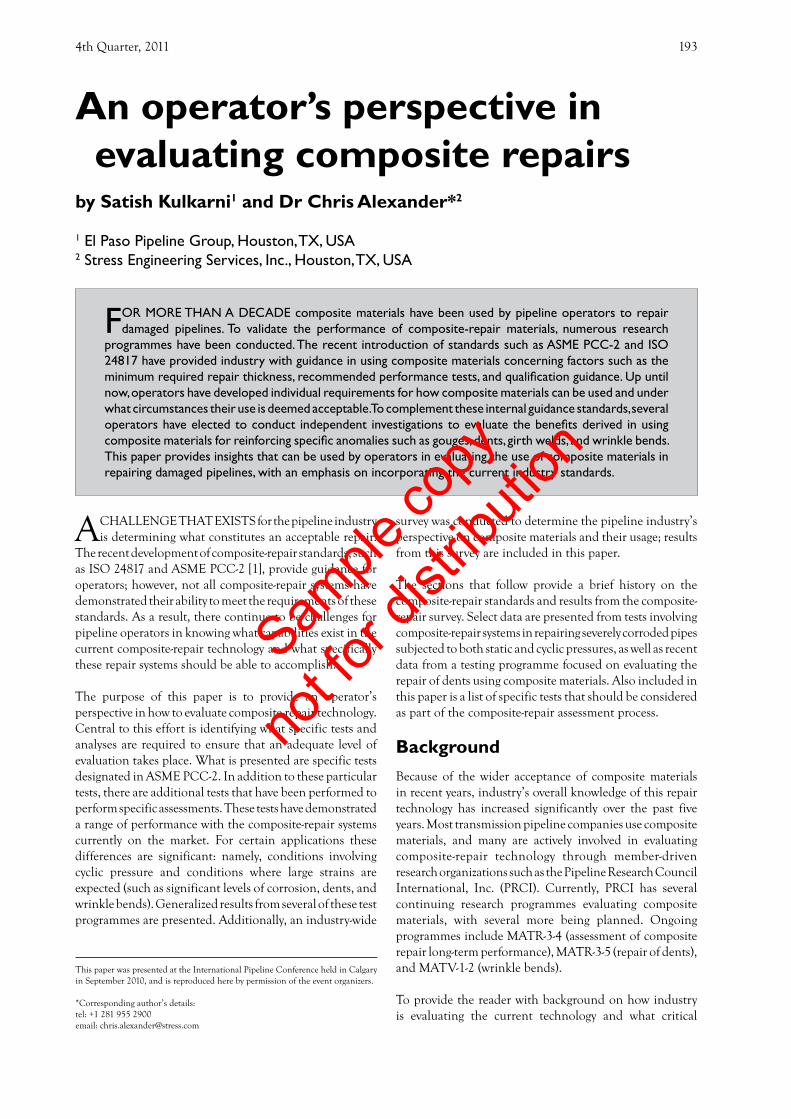
FOR MORE THAN A DECADE composite materials have been used by pipeline operators to repair damaged pipelines. To validate the performance of composite-repair materials, numerous research
programmes have been conducted. The recent introduction of standards such as ASME PCC-2 and ISO 24817 have provided industry with guidance in using composite materials concerning factors such as the minimum required repair thickness, recommended performance tests, and qualification guidance. Up until now, operators have developed individual requirements for how composite materials can be used and under what circumstances their use is deemed acceptable. To complement these internal guidance standards, several operators have elected to conduct independent investigations to evaluate the benefits derived in using composite materials for reinforcing specific anomalies such as gouges, dents, girth welds, and wrinkle bends. This paper provides insights that can be used by operators in evaluating the use of composite materials in repairing damaged pipelines, with an emphasis on incorporating the current industry standards.
by Satish Kulkarni1 and Dr Chris Alexander*2
1 El Paso Pipeline Group, Houston, TX, USA2 Stress Engineering Services, Inc., Houston, TX, USA
An operator’s perspective in evaluating composite repairs
Sample
copy
not fo
r dist
ributi
on
The Journal of Pipeline Engineering194
itself. The Composite Standards specify minimum tensile strength for the material of choice based on maximum acceptable stress or strain levels.
• Long-term performance of the composite material is central to the design of the repair systems based on the requirements set forth in the Composite Standards. To account for long-term degradation safety factors are imposed on the composite material that essentially requires a thicker repair laminate than if no degradation was assumed.
• One of the most important features of the Composite Standards is the organization and listing of ASTM tests required for material qualification of the composite material (i.e. matrix and fibres), filler materials, and adhesive. Listed below are several of the ASTM tests listed in ASME PCC-2 (note that there are also equivalent ISO material qualification tests not listed here).
• tensile strength: ASTM D 3039• hardness (Barcol or Shore hardness): ASTM D 2583• coefficient of thermal expansion: ASTM E 831• glass transition temperature: ASTM D 831, ASTM
E 1640, ASTM E 6604• adhesion strength: ASTM D 3165• long-term strength (optional): ASTM D 2922• cathodic disbondment: ASTM-G 8
With the development of standards for composite repairs, industry can evaluate the performance of competing repair
issues are worthy of attention, the following sections have been prepared. The first section concerns background information on industry standards; the second section, operator perspectives, provides background on how El Paso is evaluating the current composite technology and how these materials are used as part of El Paso’s ongoing integrity management programme.
Industry standardsFor much of the time period during which composite materials have been used to repair pipelines, industry has been without a unified standard for evaluating the design of composite-repair systems. Under the technical leadership of engineers from around the world, several industry standards have been developed, and these include ASME PCC-2 and ISO 24817 (hereafter referred to as the Composite Standards). Interested readers are encouraged to consult these standards for specific details; however, listed below are some of the more noteworthy contributions these standards are providing to the pipeline industry:
• The Composite Standards provide a unifying set of design equations based on strength of materials. Using these equations, a manufacturer can design a repair system so that a minimum laminate thickness is applied for a given defect. The standards dictate that for more severe defects, greater reinforcement from the composite material is required.
• The most fundamental characteristic of the composite material is the strength of the composite
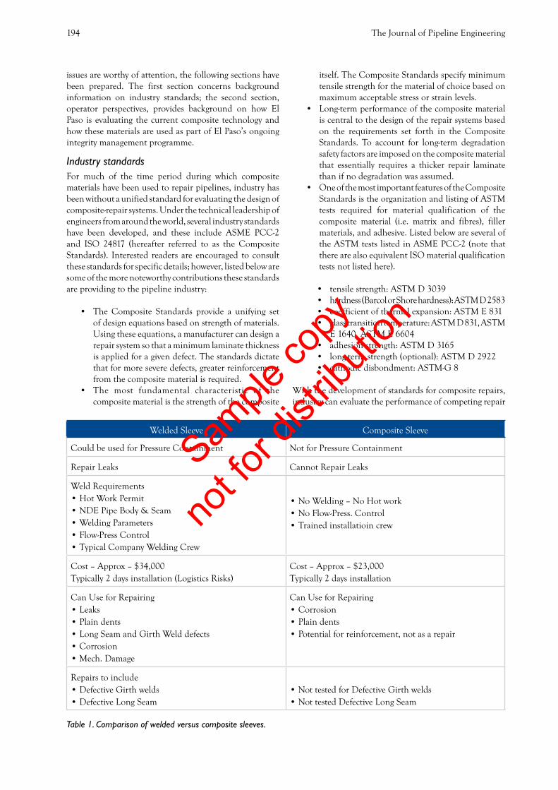
Table 1. Comparison of welded versus composite sleeves.
Welded Sleeve Composite Sleeve
Could be used for Pressure Containment Not for Pressure Containment
Repair Leaks Cannot Repair Leaks
Weld Requirements•HotWorkPermit•NDEPipeBody&Seam•WeldingParameters•Flow-PressControl•TypicalCompanyWeldingCrew
•NoWelding–NoHotwork•NoFlow-Press.Control•Trainedinstallatioincrew
Cost – Approx – $34,000Typically 2 days installation (Logistics Risks)
Cost – Approx – $23,000Typically 2 days installation
Can Use for Repairing •Leaks•Plaindents•LongSeamandGirthWelddefects•Corrosion•Mech.Damage
Can Use for Repairing •Corrosion•Plaindents•Potentialforreinforcement,notasarepair
Repairs to include•DefectiveGirthwelds•DefectiveLongSeam
•NottestedforDefectiveGirthwelds•NottestedDefectiveLongSeam
Sample
copy
not fo
r dist
ributi
on

4th Quarter, 2011 195
Table 2. Suggested operator assessment criteria based on ASME PCC-2.
Sample
copy
not fo
r dist
ributi
on
The Journal of Pipeline Engineering196
the costs will vary for each particular situation; however, the point is that composite materials can provide an economic and safe alternative to steel sleeves.
One of the challenges presented to each operator is evaluating the composite technology itself. There are more than 15 different composite-repair systems on the market, with manufacturing headquarters in both the United States and Europe. There exists confusion in what is required of each system according to standards such as ASME PCC-2. The authors have also observed composite-repair companies purporting to be compliant with ASME PCC-2, yet when questioned about requirements for compliance, some manufacturers do not have a complete understanding of the requirements. On the other side, there are several composite-repair systems that have performed very well in all testing programmes and have demonstrated their capabilities to repair a wide range and class of pipeline defects. Table 2 is presented and can be used by operators to distinguish those manufacturers who truly have systems worthy of recognition and possess the requirements necessary to repair high pressure gas and liquid transmission pipelines. Much of the contents in this table are taken from the requirements set forth in ASME PCC-2. The general observation is that if a particular manufacturer meets the requirements of ASME PCC-2, this particular system is adequately designed to repair most pipeline anomalies.
The section that follows provides information on several specific test programmes that evaluated the repair of corrosion subjected to both static and cyclic pressures. Also provided is a discussion on a recent programme where composite materials were used to repair dents subjected to cyclic pressure conditions. It should be noted that the information provided in these tests is not explicitly defined in ASME PCC-2, but is extremely important in evaluating the true limit state condition of composite-repair technology in an effort to satisfy the intent of both the pipeline codes and regulations stating that reliable engineering tests and analyses must be used to demonstrate the worthiness of composite materials for long-term performance.
Performance testingWhile performing tests to meet the minimum requirements of ASME PCC-2 is a starting point for any composite-repair system, ultimate performance cannot be established without evaluating performance relative to more aggressive testing regimes. This section of the paper presents details and results associated with three specific test programmes that include the following:
• repair of 75% corrosion in 12.75-in x 0.375-in Grade X42 pipe subjected to static burst testing
• repair of 75% corrosion in 12.75-in x 0.375-in Grade X42 pipe subjected to cyclic pressures
• repair of dents in 12.75-in x 0.375-in Grade X42 pipe subjected to cyclic pressures
systems based on a set of known conditions. It is anticipated that the Composite Standards will either be accepted in part, or in whole, by the transmission pipeline design codes such as ASME B31.4 (liquid) and ASME B31.8 (gas).
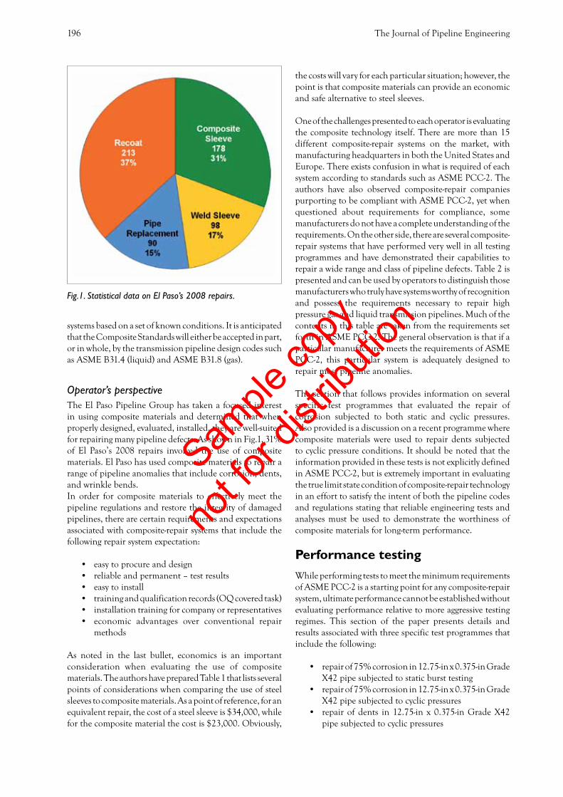
Operator’s perspectiveThe El Paso Pipeline Group has taken a focused interest in using composite materials and determined that when properly designed, evaluated, installed, they are well-suited for repairing many pipeline defects. As shown in Fig.1, 31% of El Paso’s 2008 repairs involved the use of composite materials. El Paso has used composite materials to repair a range of pipeline anomalies that include corrosion, dents, and wrinkle bends.In order for composite materials to effectively meet the pipeline regulations and restore the integrity of damaged pipelines, there are certain requirements and expectations associated with composite-repair systems that include the following repair system expectation:
• easy to procure and design• reliable and permanent – test results• easy to install• training and qualification records (OQ covered task)• installation training for company or representatives• economic advantages over conventional repair
methods
As noted in the last bullet, economics is an important consideration when evaluating the use of composite materials. The authors have prepared Table 1 that lists several points of considerations when comparing the use of steel sleeves to composite materials. As a point of reference, for an equivalent repair, the cost of a steel sleeve is $34,000, while for the composite material the cost is $23,000. Obviously,
Fig.1. Statistical data on El Paso’s 2008 repairs.
Sample
copy
not fo
r dist
ributi
on

4th Quarter, 2011 197
monitored during testing; also included in the figure are the average strain readings from the PRCI long-term study beneath the composite repairs of 12 different composite-repair systems. At the MAOP (72% SMYS or 1,778psi) the hoop strain was approximately 3,000 microstrain, compared to the average PRCI value of 3,410 microstrain at this same pressure level. Additionally, at 100% SMYS (2,470psi) the strain beneath the repair was recorded to be 5,200 microstrain, whereas the average PRCI strain at this pressure level was 5,170 microstrain. It should be noted that the PRCI data set comprises a range of composite materials that includes E-glass, carbon, and Kevlar. Also included in Fig.4 are data for a composite-repair system that did not perform adequately in reinforcing the corroded section of the pipe. These data are provided to demonstrate that not all composite-repair systems perform the same or provide the same level of reinforcement.
The failure in the test sample occurred outside the repair. The significance in the failure having occurred outside the repair is that these results indicate that the repair is at least as strong as the base pipe. Additionally, at the failure pressure the hoop strain in the reinforced corroded region was less than 1.2%, whereas the measured strains in the base pipe outside the repair were in excess of 10% (based on the final measured circumference at the failure location).
What has been observed in the test results is that not all composite materials perform equally. The authors have presented contrasting test results to make this point clear. Operators and industry at large are encouraged to use composite materials that can exceed the minimum requirements set forth in the existing standards.
Burst pressure testing on 75% corrosion samplesBurst test samples were fabricated by machining a 6-in wide by 8-in long corrosion section in a 12.75-in x 0.375-in Grade X42 pipe, as shown in Fig.2. After the machining was completed the sample was sandblasted to near-white metal. Prior to installing the composite-repair material, four strain gauges were installed in the following regions, as shown in Fig.3:
• gauge 1: installed in the centre of the corrosion region• gauge 2: installed 2in from the centre of the corrosion
region• gauge 3: installed on the base pipe• gauge 4: installed on the outside surface of the repair
Results are presented in this paper for a sample that was repaired using an E-glass material that was 0.625in thick. The sample was pressurized to failure, and burst outside the repair at 3,936psi. Figure 4 shows the strain gauge results that were
Fig.2. Schematic diagram of composite repair pipe test sample.
Sample
copy
not fo
r dist
ributi
on

The Journal of Pipeline Engineering198
Fig.3. Schematic showing location of strain gages of photo of machined region.
Fig.4. Strains measured in composite reinforced corroded pipe sample (12.75-in x 0.375-in, Grade X42 pipe with 75% corrosion).
Sample
copy
not fo
r dist
ributi
on

4th Quarter, 2011 199
however, one can definitely conclude that all composite repair systems are not equal. The study on the carbon composite system having four different pipe samples was specifically conducted by a manufacturer to determine the optimum design conditions for reinforcing the severely corroded pipe. Figure 5 shows the strains recorded in the four carbon-reinforced test samples: what is noted in this plot is that the lowest recorded mean strains occur in Pipe no.4, which also corresponds to the test sample that had the largest number of cycles to failure.
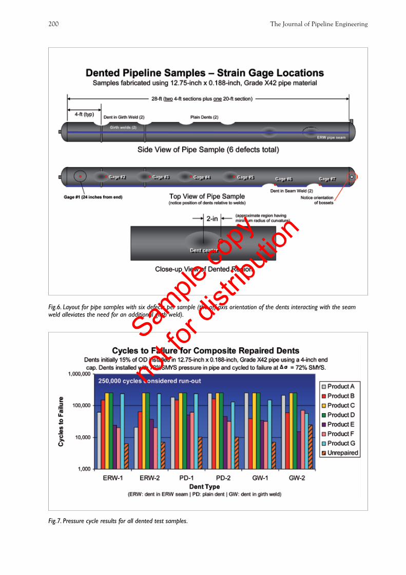
Cyclic pressure testing on dented pipe samplesIn response to past successes, a Joint Industry Programme (JIP) was organized to experimentally evaluate the repair of dents using composite materials. This programme was co-sponsored by the Pipeline Research Council International, Inc. and six manufacturers, and involved testing seven different repair systems. Additionally, a set of unrepaired dent samples was also prepared to serve as the reference data set for the programme. The dent configurations included plain dents, dents in girth welds, and dents in ERW seams. Testing involved installing 15% deep dents (as a percentage of the pipe’s outside diameter) where the dents were cycled to failure or 250,000 cycles, whichever came first. The dents were created using a 4-in diameter end cap that was held in place during pressurization. The test samples were made using 12.75-in x 0.188-in, Grade X42 pipe with a pressure cycle range equal to 72% SMYS. Strain gauges were also placed in the dented region of each sample and monitored periodically during the pressure-cycle testing. Figure 6 provides a schematic of the test samples, while Fig.7 is a bar chart showing graphically the cycles to failure.
Cyclic pressure testing on 75% corrosion samplesMost of the experimental research associated with the composite repair of corroded pipelines has focused on burst tests. The general philosophy has been that in the absence of cyclic pressures during actual operation, there are few reasons to be concerned with qualifying composite repairs for cyclic conditions. One could argue that only liquid transmission pipelines need to be concerned about cyclic pressures. However, recent studies have indicated that for severe corrosion levels (of the order of 75%) there is a need to take a closer look at the ability of the composite to provide reinforcement. The case study presented here was actually preceded by a series of tests using E-glass materials that evaluated the number of pressure cycles to failure in reinforcing 75% corrosion in a 12.75-in x 0.375-in Grade X42 pipeline (sample as the geometry shown in Fig.2, with Fig.3 showing the strain gauge positions). The test samples were pressure cycled at a pressure range of 36% SMYS (i.e. differential of 894psi for this pipe size and geometry).
The tests were performed on six different composite systems that included the following cycles to failure:
• E-glass system: 19,411 cycles to failure• E-glass system: 32,848 cycles to failure• E-glass system: 140,164 cycles to failure• E-glass system: 165,127 cycles to failure• E-glass system: 259,357 cycles to failure• Carbon system: 532,776 cycles to failure
Minimal information is provided with the above data (for example, no information was provided on thickness, composite modulus, filler materials, fibre orientation, etc.);
Fig.5. Measured strain range in 75% corroded test sample (test sample cycled at ΔP = 36% SMYS, data plotted at start-up).
Sample
copy
not fo
r dist
ributi
on
The Journal of Pipeline Engineering200
Fig.7. Pressure cycle results for all dented test samples.
Fig.6. Layout for pipe samples with six defects per sample (the off-axis orientation of the dents interacting with the seam weld alleviates the need for an additional girth weld).
Sample
copy
not fo
r dist
ributi
on

4th Quarter, 2011 201
front page of the www.compositerepairstudy.com website used both to collect data and post the results. Interested readers are encouraged to visit the website for additional details and results, including postings from the composite manufacturers themselves.
The questions that were developed for the survey were based on input received from pipeline companies, and specifically from PRCI members. Topics of interest ranged from type of repair materials to the range of repaired pipeline anomalies. Provided below are responses to five of the 11 questions posed to operators; the details provided include the statistical data, as well as pie charts showing the distribution of responses.
Number of composite repairsQuestion: Estimate the total number of composite repairs that will be used in the next 12 months. Figure 9 graphical shows the responses for this question.
• None [3 votes] • 1 - 10 repairs [11 votes]• 11 - 25 repairs [6 votes] • 26 - 50 repairs [7 votes] • 51 - 75 repairs• 76 - 100 repairs [1 vote]• More than 100 repair [4 votes]
The following general observations are made in reviewing the pressure cycle data:
• The average cycles to failure for the unrepaired dent samples were 10,957 cycles. The target cycles to failure for the unrepaired dents was 10,000 cycles.
• Two of the seven systems had 250,000 cycles with no failures, and included a carbon/epoxy system and a pre-cured E-glass system.
• The minimum cycles to failure was recorded for System E that had average fatigue life of 34,254 cycles.
To be effective in repairing dents subjected to cyclic pressures, a composite repair system should demonstrate an ability to increase fatigue life by a factor of at least ten times that of the unreinforced dent samples, and a factor of 20 for high-cycle applications. For the programme presented here, this implies fatigue lives of at least 100,000 cycles, or 200,000 cycles for high-pressure applications.
Industry survey To determine industry’s perspective on the use of composite materials, an on-line survey was conducted of PRCI members and readers of Hart’s Pipeline & Gas Technology. The survey was completed in October, 2009, and included input from 18 pipeline companies. Figure 8 shows the
Fig.8. Composite survey website for industry and manufacturers.
Sample
copy
not fo
r dist
ributi
on

The Journal of Pipeline Engineering202
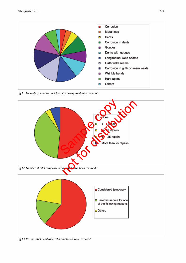
• Dents [5 votes]• Corrosion in dents [11 votes]• Gouges [8 votes]• Dents with gouges [11 votes]• Longitudinal weld seams [14 votes]• Girth weld seams [15 votes]• Wrinkle bends [12 votes]• Hard spots [8 votes]• Others [3 votes]
Number of composite repairsQuestion: How many total composite repairs have been removed by your company? Figure 12 graphical shows the responses for this question.
• None [16 votes]• 1 - 5 repairs [12 votes]• 6 - 19 repairs • 11 - 25 repairs [1 vote]• More than 25 repairs [2 votes]
Types of geometry repaired using compositesQuestion: Do your composite repair procedures allow for the repair of the following pipe geometries? Figure 10 graphical shows the responses for this question.
• Straight pipe [30 votes]• Elbows [19 votes]• Tees [16 votes]• Field bends [18 votes]• Others [2 votes]
Types of anomaly repaired using compositesQuestion: Which of the following anomaly type repairs are not permitted by your company using composite materials? Figure 11 graphical shows the responses for this question.
• Corrosion [4 votes]• Corrosion in girth or seam welds [14 votes]• Metal loss [4 votes]
Fig.9. Number of composite repairs to be used in the next 12 months.
Fig.10. Composite repairs allowed for the repair of the following pipe geometries.Sam
ple co
py
not fo
r dist
ributi
on
4th Quarter, 2011 203
Fig.11. Anomaly type repairs not permitted using composite materials.
Fig.12. Number of total composite repairs that have been removed.
Fig.13. Reasons that composite repair materials were removed.
Sample
copy
not fo
r dist
ributi
on

The Journal of Pipeline Engineering204
petroleum gas, anhydrous ammonia and alcohols. ASME B31.4, New York.
3. American Society of Mechanical Engineers, 2003. Gas transmission and distribution piping systems. ASME B31.8, New York.
4. American Society of Mechanical Engineers, 2004. Rules for construction of pressure vessels, Section VIII, Division 2 - Alternative Rules. New York.
5. D.R.Stephens and T.J.Kilinski, 1998. Field validation of composite repair of gas transmission pipelines. Final report to the Gas Research Institute, Chicago, Illinois, GRI-98/0032, April.
6. F.Worth, 2005. Analysis of Aquawrap for use in repairing damaged pipeline: environmental exposure conditions, property testing procedures, and field testing evaluations. Air Logistics Corporation, Azusa, California, September 28.
7. Pipeline safety: gas and hazardous liquid pipeline repair. Federal Register, Vol.64, No.239, Tuesday, December 14, 1999, Rules and Regulations, Department of Transportation, Research and Special Programs Administration, Docket No. RSPA-98-4733; Amdt. 192-88; 195-68 (Effective date: January 13, 2000).
8. American Society of Mechanical Engineers, 2006. STP-PT-005: Design factor guidelines for high-pressure composite hydrogen tanks. New York.
9. ASTM International, 2001. ASTM D2992: Standard practice for obtaining hydrostatic or pressure design basis for fiberglass (glass-fiber-reinforced thermosetting-resin) pipe and fittings.
10. American Society of Mechanical Engineers, 2004. Boiler and pressure vessel code, Section VIII, Division 3: Alternative rules for construction of high pressure vessels. New York.
11. C.Alexander and S.Kulkarni, 2008. Evaluating the effects of wrinkle bends on pipeline integrity. Proc. IPC 2008, paper no. IPC2008-64039, 7th International Pipeline Conference, September 29-October 3, 2008, Calgary, Alberta, Canada.
Reasons for composite repair removalQuestion: For what reasons were the composite repair materials removed? Figure 13 graphical shows the responses for this question.
• Considered temporary [11 votes]• Failed in service due to disbonding of composite
material [3 votes]• Others [4 votes]
ConclusionsThis paper has provided insights on how composite materials can be used by pipeline operators to repair damaged pipelines, with an emphasis on incorporating the current industry standards. Over the past decade several industry-sponsored programmes have focused on looking at the available composite repair technology and determining if any pertinent limitations exist. Additionally, what is earned from the survey data presented in this paper is that the pipeline industry is using composite materials and that, for many of these companies, composite repair systems are an important part of their integrity-management programmes. It was the intent of the authors to provide industry with a systematic means for assessing repair technology and how standards such as ASME PCC-2 can be integrated into this process.
References1. American Society of Mechanical Engineers, 2008.
ASME Post construction SC-repair & testing, PCC-2, Repair Standard, Article 4.1: Non-metallic composite repair systems for pipelines and pipework: high risk applications. New York.
2. American Society of Mechanical Engineers, 2003. Liquid transportation system for hydrocarbons, liquid
Sample
copy
not fo
r dist
ributi
on

4th Quarter, 2011 205
Enbridge Pipelines Inc. completed construction of the 138-km NPS 36 Line 4 Extension oil pipeline in the
spring of 2009. The project is based in Alberta and required ten mainline hydrostatic tests. These tests were required based on the scarcity of water sources along the pipeline right-of-way and complications faced during execution of the winter hydrostatic-testing programme.
The operating company also completed construction of the Canadian portion of the Alberta Clipper Expansion oil pipeline in the winter of 2009. From Hardisty, Alberta, to the Canada-US border near Gretna, Manitoba, this 1,081-km NPS 36 oil pipeline was completed over three consecutive
construction seasons. The hydrostatic-testing programme required 47 hydrostatic test sections and was completed in five months (May to October 2009).
During construction and hydrostatic testing of the Line 4 Extension project, many lessons were learned that were implemented for the Alberta Clipper Expansion project, the most important of which was the importance of fully ground-evaluating water sources. This lesson was implemented for the Alberta Clipper Expansion project, leading to an efficient hydrostatic-testing programme with no unforeseen water-source issues.
This paper provides a cost-benefit assessment of pre-planning versus the costs of delays to the execution of hydrostatic testing, and identifies specific areas where pre-planning can minimize the risk to a successful hydrostatic-testing programme.
This paper was presented at the International Pipeline Conference held in Calgary in September 2010, and is reproduced here by permission of the event organizers.
* Corresponding author’s detailstel: +1 403 212 8388email: [email protected]
LARGE HYDROSTATIC-TEST programmes require extensive pre-planning to avoid increased costs and delayed schedules. Recently, Enbridge Pipelines Inc. completed construction and testing of more
than 1,200 km of an NPS 36 oil pipeline for the Line 4 Extension Project and the Canadian portion of the Alberta Clipper Expansion Project over three construction seasons. 57 mainline hydrostatic tests were successfully completed and approved by the National Energy Board. Following the first construction and hydrostatic-testing season, many lessons were learned that were implemented for hydrostatic testing during the second construction season.
The most important aspect of large pipeline hydrostatic-test programmes is locating and securing water sources. Extensive ground evaluation must be preformed to adequately determine locations, volumes, and access to water sources. Once potential sources are identified, water-quality and environmental issues must be assessed, which leads to applying for and obtaining the necessary permits for water withdrawal and discharge. Leaving an important item such as water sources to be “field determined” can lead to unanticipated complications, schedule delay, and increased construction costs. Water sources are just one of the many important pre-planning activities that must be given adequate attention before the start of pipeline construction to successfully and efficiently manage a large pipeline hydrostatic-test programme. Many projects only complete high-level desktop based hydrostatic-test planning during the detailed design phase of a project. However, the potential cost and schedule impacts far outweigh the extra costs required to complete proper pre-planning during the detailed engineering phase of a project.
by Andrew Keith Bennett*1 and Everett Clementi Wong2
The importance of pre-planning for large hydrostatic test programmes
1 WorleyParsons Calgary, Calgary, AB, Canada2 Enbridge Pipelines Inc., Edmonton, AB, Canada
Sample
copy
not fo
r dist
ributi
on

platinum sponsor
organizers
silver sponsor gold sponsors
19–21 March 2012, Bahrain
Held under the Patronage of His Excellency Dr. Abdul Hussain bin Ali Mirza, Minister of Energy, Kingdom of Bahrain
Gulf Convention Centre, Bahrain
www.pipelineconf.com
ConferenCeSeven technical streams covering a wide range of subjects will run over the two and a half day event (and be presented by industry leaders).
Join leaders in the international pipeline industry as they converge for the Best Practice in Pipeline operations and integrity Management Conference and exhibition in Bahrain.
exhiBitionA comprehensive exhibition will be part of the event, allowing companies from around the world to showcase their products and services. Contact us today to book your space.
registrations are now open – make sure you attend this landmark event.
networkinGThroughout the event there will be ample opportunities to network with participants to further your business relationships. Meet with industry leaders from around the world.
WGlobalWebb
bahrain_conf. announcement_ad.indd 1 3/06/11 8:44 AM
Sample
copy
not fo
r dist
ributi
on

4th Quarter, 2011 207
• depth profile• access to the water source• water quality• discharge location
The starting point of any hydrostatic testing programme, whether it is for one test or multiple tests, is the water source. Typically, high-quality water minimizes the risk of pipeline corrosion, but because water volumes for large-diameter pipelines are significant, municipal potable water supplies are insufficient or have a significant cost, and therefore large surface-water sources are required. Large water bodies or rivers are not always easily accessible or even exist along pipeline rights-of-way; even when they appear to be present on a map or aerial image, they can often be deceptive.
Some watersheds are protected by local or national regulatory agencies. For instance, on the Alberta Clipper Expansion project, several potential water sources were deemed protected under the Ducks Unlimited Conservation programme. In another case, a particular watershed was deemed for recreational water, meaning withdrawal and discharge required a Transport Canada permit which would take three months to acquire.
Water source volume must be assessed, as one of the lessons learned on the Line 4 Extension project illustrates. One selected water source was a lake more than 2 km wide, although the majority of the lake turned out to be less than 1 m deep. While the volume of water needed was still less than a fraction of the lake’s volume, effectively pumping the water at the desired flow rate required a floating pump to be located at least 0.5 km from shore to have sufficient depth for pumping. The unanticipated placement of the floating pump and associated fill pipeline added several unplanned days to the hydrostatic-testing programme. When it was discovered that no suitable locations along the shore of the lake were deep enough to effectively pump, an application was prepared to dig a small sump at the shoreline; however, the timeline for receiving approval for the application was several months.
Potential water sources initially identified from maps and aerial imagery must have their depths checked (unless the source depth is known) because looks can be very deceptive, especially on the Canadian prairies. Depths can be checked during the summer by boat or during the winter by auguring holes in the ice. Suitable pumping locations and depths also need to be assessed. In addition, both rivers and lakes can have significant seasonal fluctuations in depth and flow rate, which need to be considered based on the planned timing of water withdrawal.
During the ground evaluation exercise to determine water levels, several other important aspects of the water source should also be assessed. For instance, access to the potential water sources from the pipeline right-of-way needs to be determined.
Costs of delays vs the cost of pre-planning
Historically, pre-planning hydrostatic-test programmes focused primarily on maximizing the length of hydrotest sections, which are bound by company specifications on maximum length and on maximum strength test pressures according to the appropriate codes. The location of water sources and their usable volumes are usually assessed based on historical data, and these desktop assessments are later “field determined”. A common term used during the detailed-design phase of large pipeline projects is that outstanding design issues will be “field determined”. Often, pre-planning for hydrostatic-test programmes is done as a desktop exercise because sending resources into the field during detailed engineering with the sole purpose of evaluating water sources can be seen as unnecessarily expensive or unimportant.
Hydrostatic testing is one construction activity which can and will be determined in the field, but minimizing the amount of field determination during construction is especially important. Fully planning ahead of time is critical to ensure hydrostatic-test programmes are pragmatic and cost-effective. Trying to determine water sources, acquire permits, and plan for contingencies during the pipeline construction process can lead to expensive decisions being made on the basis of schedule rather than cost; schedule is usually the driving factor during large pipeline construction projects. Many issues that can arise during hydrostatic testing during construction can be easily addressed by dedicating resources to properly pre-planning hydrostatic-test programmes.
Big-inch hydrostatic test crews typically consist of a foreman, straw boss, 6-10 labourers, a welder, a welder’s helper, pick-up trucks, sidebooms, fill pumps, squeeze pumps, a test shack, and a boiler for winter testing. Including inspection personnel and indirect costs, testing can cost anywhere from $20,000 to $40,000 a day. Lost production or idle days over the course of a large pipeline project can easily add up to hundreds of thousands of dollars or more for the pipeline owner.
The costs associated with full ground evaluation and pre-planning for a large hydrostatic-test programmes before construction are minimal compared to the potential costs associated with delayed construction or delayed on-stream dates for pipelines. Depending on the size and number of potential water sources for the specific project, a full ground evaluation and pre-planning exercise can usually be undertaken for less than the cost of one lost day of production for the hydrostatic test crew.
Water sourcesThe following assessments must be performed on potential water sources to assess their suitability:
• determination of protected watersheds• total pumpable volume
platinum sponsor
organizers
silver sponsor gold sponsors
19–21 March 2012, Bahrain
Held under the Patronage of His Excellency Dr. Abdul Hussain bin Ali Mirza, Minister of Energy, Kingdom of Bahrain
Gulf Convention Centre, Bahrain
www.pipelineconf.com
ConferenCeSeven technical streams covering a wide range of subjects will run over the two and a half day event (and be presented by industry leaders).
Join leaders in the international pipeline industry as they converge for the Best Practice in Pipeline operations and integrity Management Conference and exhibition in Bahrain.
exhiBitionA comprehensive exhibition will be part of the event, allowing companies from around the world to showcase their products and services. Contact us today to book your space.
registrations are now open – make sure you attend this landmark event.
networkinGThroughout the event there will be ample opportunities to network with participants to further your business relationships. Meet with industry leaders from around the world.
WGlobalWebb
bahrain_conf. announcement_ad.indd 1 3/06/11 8:44 AM
Sample
copy
not fo
r dist
ributi
on
The Journal of Pipeline Engineering208
proposed water sources. In the case of the Line 4 Extension project, water for several water sources was required to be discharged directly back into the water source to ensure water levels did not drop. Typically, discharging directly back into a water body requires more testing than if the water is discharged back to land. The unanticipated requirement of the water withdrawal and discharge permit led to filtration being required for one of the test sections. Filtration was an unanticipated cost because initial planning was always to discharge the test water to land.
Some regulations require spent hydrotest water to be discharged to land with no way for the water to flow back to a watercourse. This was the case for the Alberta Clipper Expansion project for water withdrawn from Eagle Creek. Specific permit conditions need to be identified early so they do not come as a surprise during construction. This can be done through discussions with the regulator or by early applications during the pre-planning process.
Water sources need to be fully evaluated before the start of construction to avoid last-minute surprises that can lead to delays and additional project costs. The lessons learned and experience gained during the implementation of the Line 4 Extension project hydrostatic-test programme were applied to the hydrostatic-test programme for the Alberta Clipper Expansion project. All of the water sources for the Alberta Clipper Expansion project were fully evaluated to assess volumes and access and discharge locations, and to establish if any testing would be required and to make early applications for water withdrawal and discharge.
General hydrostatic testing contingency planning
There are three possible outcomes of a hydrostatic test:
• successful test• pipe failure• pressure will not stabilize during strength or leak test
A successful test is the goal of all hydrostatic tests, but the second and third possible outcomes result in a course of action being taken that, if not pre-planned, can lead to schedule delays, cost impacts, and regulatory scrutiny. Pipe failure, although rare, does happen during hydrostatic testing and typically comes as a major surprise to all involved, which often leads to confusion over the immediate course of action to be taken. Most companies have hydrostatic-test standards and procedures that deal with pipe failure, but these standards and procedures need to be reviewed for their relevance to the specific project and reviewed with the contractor to ensure a correct and timely reaction takes place.Pressure not stabilizing in a test section is much more likely than pipe failure, but can also catch companies off guard. The typical course of action when this happens is
During the Line 4 Extension project, regulatory authorities approved a large water source in close proximity to the pipeline right-of-way. However, the source could not be used because none of the landowners between the right-of-way and water source would allow access for the placement of a fill line or pumps. This scenario was not anticipated and led to changing water sources during construction. Access agreements need to be determined and worked out with landowners well before construction begins.
Consideration must also be given to the placement of fill lines when determining access to water sources not directly on the right-of-way. One potential water source considered for the Line 4 Extension project required crossing a rail spur for the fill line; this water source was quickly ruled out.
Water quality affects the suitability of the water source; therefore, another task during early ground evaluation is taking water samples. Water quality needs to be assessed for various characteristics: in terms of pipeline integrity, water with very high or very low pH can lead to corrosion problems and high levels of suspended solids can clog instrumentation lines and damage valve seals. Total dissolved solids, salts, pH, trace metals, biota, and suspended solids could adversely affect the land or other watersheds when test water is discharged [1]. Therefore, water-quality testing is required to determine the suitability for discharge to land or to set an environmental baseline for returning the water back to the water source. Tests should also be conducted to determine if any existing contaminants are in the water. Local regulatory authorities limit the withdrawal and release of water based on these and other characteristics, and discussions with the local regulatory authorities are therefore necessary.
The second major step in evaluating ground-water sources is determining water discharge areas. Will water be discharged back into the original water source, another water source, or back to land? These are all questions that need to be determined during pre-planning. One typical scenario is to withdraw water at one end of a pipeline and continuously move the water from one test section to another test section further away from the original water source (known as ‘shunting’) and discharge at the far end of the pipeline once the last test section is completed. This can lead to many potential complications, especially with today’s more stringent environmental regulations, because transfer of water from one watershed to another is often prohibited. This change could significantly affect the hydrostatic test plan because the project is forced to transfer water back though all test sections to be discharged near the original water source, costing significant time and money.
Once water sources have been evaluated for depth, access, discharge locations, and quality, the applicable environmental regulatory bodies should be contacted to be advised of the proposed plan, and to highlight if there are any other requirements or issues associated with the
Sample
copy
not fo
r dist
ributi
on

4th Quarter, 2011 209
than anticipated. The testing schedule was delayed so that this particular water withdrawal would not take place until after a two-week construction break. This particular area had no other available water sources and a decision was made to dig a large temporary holding pond 5 m deep. The temporary holding pond was dug and the water required for the test was withdrawn from the water source. Following the two-week break, the ice depths were checked on the original water source. The water source was mostly frozen solid with less than 10 cm of water in the deepest part of the lake. More than 70 cm of ice had built-up on the lake and temporary holding pond. To melt the ice and to regain more usable water from the holding pond, the water underneath the ice was circulated through a heater. Had the required water not been put into the deep temporary holding pond, there would not have been any water available for testing. Trucking in the volume of water required for the test would have cost more than $500,000.
Standard practice during winter testing is to begin filling a test section with a hot slug. A hot slug is typically 35°C or warmer and the pipeline is filled more slowly than a standard filling operation. The hot slug warms the frozen backfill around the pipe in an attempt to achieve equilibrium during testing between the ground and water temperatures. There are many rules-of-thumb and variables that go into determining hot-slug temperatures and volumes. Following the hot slug, the pipeline is generally filled with heated water until a consistent temperature is seen flowing out of the far end of the test section.
During the Line 4 Extension project, a short test section was filled with water that was too warm. After being left to stabilize overnight, there was still a temperature differential between the soil and the pipe of more than 15°C. This test section was monitored for five days before the pressure started stabilizing and a successful hydrostatic test could be achieved.
Very tight control needs to be taken over hot-slug temperatures and fill rates to avoid filling test sections with water that is too warm, which makes it almost impossible to perform a successful hydrostatic test.
During pre-planning for hydrostatic testing, plans for monitoring hot-slug and fill temperatures should be made to ensure the test sections do not get filled with water that is too warm. Also contingency plans should be made in the event that a test section gets filled too warm, based on the specific project variables. Dewatering a test section and refilling can often be more cost effective than waiting on a test section to stabilize. However, these are very difficult decisions to make in the field during construction, and having a plan in place to deal with such instances will improve overall project cost and schedule.
to attempt to reconcile the pressure drop with a drop in water temperature in the pipeline. This seems like a relatively easy concept but, in reality, it can be quite difficult to accomplish and even tougher to get signed-off by the pipeline owner. In a long hydrotest section, the correlation assumes that the bulk temperature of the water is homogenous; however, experience has shown that this is not the case, especially during winter hydrostatic tests. In the winter, the point temperature of the water, as measured on the outside wall of the pipe can vary by up to 5°C at each end of the test section. Furthermore, the standard temperature chart recorders that are most often used are subject to interpretation leading to an accuracy of +/-1°C. Half a degree can mean the difference between correlating and not correlating a pressure change to a change in temperature. Another possibility is a leak causing the pressure drop during testing, which can be very difficult to detect.
During the pre-planning of a hydrostatic test programme, a step-by-step procedure should be developed to deal with test section pressure stabilization issues.
• what are the stabilization criteria?• what is the procedure for collecting data to perform
a pressure temperature correlation?• how should the correlation be performed; what
method will be used?• should the correlation work out mathematically,
who is required to approve it before dewatering the affected test section?
• if the correlation does not work, what procedures will be used to try and identify the location of the potential leak?
These are all questions that take time to answer during construction, but which can all be answered before the hydrostatic testing programme begins. Having a pre-planned step-by-step process in place can improve project costs significantly and minimize schedule delays.
Winter testingWinter hydrostatic testing is more complicated than summer testing, and requires additional issues to be pre-planned during the detailed design of the pipeline.
The largest difference for water sources between summer and winter testing is the ice level. Ice depths can exceed 1 m, depending on the severity of the winter. Ice depth reduces the available volume of water from lakes and can completely freeze rivers. One scenario encountered during the Line 4 Extension project illustrates this issue. The water source selected was relatively small and averaged less than 1 m in depth. Based on the surface area, less than 1 cm of water depth was required to fill the largest test section. A very cold winter was encountered and the ice depth began to build up faster
Sample
copy
not fo
r dist
ributi
on

Pipelines International Premium is the international oil and gas pipeline industry’s foremost in-depth source of information, comprising a digest ofhigh-quality papers covering the latest technologyand reviews of the pipeline industry worldwide, anda comprehensive project database. It is comprised of:Pipelines International Digest which provides a month-ly update of papers covering all areas of theindustry – from key projects, and engineering andconstruction issues, to environmental, regulatory,legal and fi nancial issues.
Pipelines International Projects which allows subscribers to access a searchable database of completed andcurrent projects.
Subscribe or get a free 14 day trial now atwww.pipelinesinternational.com/premium
The new online information servicethat unlocks the secrets of the global pipeline industry
PIN_Premium_FP.indd 1 15/06/10 3:23 PM
Sample
copy
not fo
r dist
ributi
on
4th Quarter, 2011 211
ConclusionPre-planning for large hydrostatic-test programmes is an essential element in the successful execution of large pipeline projects. The costs of pre-planning are far outweighed by the potential costs of delays and uncertainty during construction. The following list summarizes the major items that should be fully addressed as a minimum before the start of construction, and not be left to be “field determined”:
• Identify potential water sources evaluate if they are in protected watersheds
• Evaluate water sources determine depths to establish volumes determine pump locations determine access requirements take water samples to determine water quality and environmental baselines determine discharge locations
• Communicate with Regulatory Agencies schedule preliminary meetings to determine any unforeseen requirements obtain water withdrawal and discharge permits
• Contingency plans pipe failure pressure drop during test
• Winter testing anticipated ice depths hot-slug size and temperature fill temperatures
• Test-head logistics determine test-head requirements and movement for hydrostatic testing programme plan for overlapping test sections
Reference1. Tera Environmental Consultants (Alta.) Ltd and
CH2M Gore and Storrie Ltd, 1996. Hydrostatic test water management guidelines. Canadian Association of Petroleum Producers (CAPP), Canadian Energy Pipeline Association (CEPA), Calgary.
Hydrostatic test head logisticsOn large pipeline projects such as the Alberta Clipper Expansion project, sourcing and management of hydrostatic test heads are important factors in efficiently executing the hydrostatic-test programme. Shortage of test heads has cost implications in terms of standby and delays to final tie-ins.
The Alber ta Clipper Expansion project used 32 hydrostatic test heads for its 47 test sections. The hydrostatic-test programme was complicated by the fact that hydrotests in each Province were conducted concurrently and the terms and conditions of water withdrawal discharge permits in some locations did not allow the water to be returned to its source. On a typical construction spread, if there are more than three hydrotest sections, the layout of the sections has to be such that the section closest to the water source is the longest and the last section (into which the test water is shunted) is the shortest. Usually, shunting from one section to another section ties-up six test heads: one pair contains the water to be shunted, another pair receives the water, and the final pair is used as set-up for the next test section.
The length of the test head should be enough to ensure that two to three fill pigs can properly fit into the test head. The test-head’s nozzle placement with respect to the fill pigs should be configured so as to allow one pig to be launched at a time. A hydrostatic-test programme that requires shunting will require one fill pig to be launched ahead of the water and a dewatering pig to be propelled by compressed air to shunt to the next section once the test is completed.
One issue that is often over looked when setting-up test heads is making sure that test sections overlap each other. Overlapping test sections minimizes the number of final tie-in welds between the test sections that do not get hydrostatically tested. If test sections are not overlapped, a pre-tested pup must be installed between the sections. Pups require two final tie-in welds, both of which will not be hydrostatically tested. Managing and tracking the pups used for the final tie-ins between test sections can be a difficult and unnecessary task; using pups for final tie-ins between test sections also complicates ‘Leave-to-open’ paperwork and hydrostatic test records.
Pipelines International Premium is the international oil and gas pipeline industry’s foremost in-depth source of information, comprising a digest ofhigh-quality papers covering the latest technologyand reviews of the pipeline industry worldwide, anda comprehensive project database. It is comprised of:Pipelines International Digest which provides a month-ly update of papers covering all areas of theindustry – from key projects, and engineering andconstruction issues, to environmental, regulatory,legal and fi nancial issues.
Pipelines International Projects which allows subscribers to access a searchable database of completed andcurrent projects.
Subscribe or get a free 14 day trial now atwww.pipelinesinternational.com/premium
The new online information servicethat unlocks the secrets of the global pipeline industry
PIN_Premium_FP.indd 1 15/06/10 3:23 PM
Sample
copy
not fo
r dist
ributi
on
CONFERENCE ORGANIZERS
SUPPORTERS
21–24 May 2012Crowne Plaza Hotel, Kuala Lumpur, Malaysia
21-22 MAY 2012CONFERENCE
21-22 MAY 2012EXHIBITION
23-24 MAY 2012TRAINING COURSES
The world renowned Pipeline Pigging and Integrity Management Conference will come to Asia in 2012.
The Asia Pacific Pipeline Pigging and Integrity Management Conference will allow pipeline professionals in the region access to an exciting programme of papers, great networking events and the latest technology on display at the exhibition.
If you are responsible for the management of oil and gas pipelines, make sure you don’t miss this event.
Plan to be there: www.clarion.org or call us at +61 3 9248 5100
PPIM_Asia_2012.indd 1 10/01/12 4:16 PM
Sample
copy
not fo
r dist
ributi
on

4th Quarter, 2011 213
Numerical analyses
In this paper, we consider pipe samples with a length (L) to diameter (D) ratio equal to 10, and for two different
load cases:
(a) the sample is loaded by axial tension and afterwards, keeping the applied axial load constant, it is loaded with external pressure up to collapse;
(b) the sample is loaded by axial tension and afterwards, keeping the axial displacement of the sample ends constant, it is loaded with external pressure up to collapse.
Even though the hardening of the material does not have any influence on the external collapse pressure of the pipes when the applied load is only external pressure [2], in this case [axial tensile load + external pressure] we also investigated the effect of the material hardening (Et) on the results.
For our analyses we considered a 7-in diameter pipe and two material grades: Grade 55 and Grade 80. We included in our models a constant ovality of 0.5%.
The finite-element models were developed using the shell element MITC4 [3-5] which incorporates shear deformation, while the ADINA [6] code was used for the analyses. We considered a simple bilinear material model with hardening modulus Et. The reliability of these models was established via several validations that are discussed in Refs. 2 and 7-10. Regarding the boundary conditions, one of the sample ends was modelled as fixed and the other one was given one axial degree of freedom.
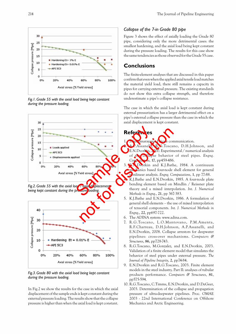
Collapse of the 7-in Grade 55 pipeIn this analysis we considered two hardening cases:
Et = E/100Et = E/10,000
where E is the Young’s modulus of the steel.
In Fig.1 we show the results for the case in which the axial load is kept constant during the external pressure loading: it is clear that for the analysed case, when both hardenings are considered, the pipe remains with a not insignificant capacity for carrying external pressure after it yields in axial tension. The figure also shows that the hardening effect is only significant for axial loads close to the yield load.
*Author’s contact details:tel: +54 11 4807 8348email: [email protected]
IT IS WELL KNOWN that, when steel pipes are subjected to axial tensile loads, their external collapse pressure diminishes. When calculating the collapse pressure of casings using the standard API 5C3, even
though the formulas are not applicable for axial tensile stresses up to the material yield stress, it is clear that the predicted collapse pressure tends to zero when the applied axial tensile stress tends to the material yield stress (see Figs 1 to 3). When calculating the collapse pressure of subsea pipeline systems using the standard DNV OS-F101, the external collapse pressure is zero when the applied axial tensile stress equals the material yield stress.
However, it has been observed that even when the applied axial tensile stress matches the material yield stress, there is still a remaining capacity in the pipes for carrying external pressure [1]. In this paper we investigate the above assertion and quantify, using finite-element models, the collapse of steel pipes that are first subjected to axial tensile load and afterwards to external pressure.
The finite-element analyses that we present here confirm that, even when the applied axial tensile load matches the material yield load, there still remains a not-negligible capacity in the pipes for carrying external pressure.
by Dr Rita G Toscano and Dr Eduardo N Dvorkin*
SIM&TEC S.A., Buenos Aires, Argentina
Collapse of steel pipes under external pressure and axial tension
CONFERENCE ORGANIZERS
SUPPORTERS
21–24 May 2012Crowne Plaza Hotel, Kuala Lumpur, Malaysia
21-22 MAY 2012CONFERENCE
21-22 MAY 2012EXHIBITION
23-24 MAY 2012TRAINING COURSES
The world renowned Pipeline Pigging and Integrity Management Conference will come to Asia in 2012.
The Asia Pacific Pipeline Pigging and Integrity Management Conference will allow pipeline professionals in the region access to an exciting programme of papers, great networking events and the latest technology on display at the exhibition.
If you are responsible for the management of oil and gas pipelines, make sure you don’t miss this event.
Plan to be there: www.clarion.org or call us at +61 3 9248 5100
PPIM_Asia_2012.indd 1 10/01/12 4:16 PM
Sample
copy
not fo
r dist
ributi
on
The Journal of Pipeline Engineering214
Collapse of the 7-in Grade 80 pipeFigure 3 shows the effect of axially loading the Grade 80 pipe, considering only the more detrimental cases: the smallest hardening, and the axial load being kept constant during the pressure loading. The results for this case show the same tendencies as those observed for the Grade 55 case.
ConclusionsThe finite-element analyses that are discussed in this paper confirm that even when the applied axial tensile load matches the material yield load, there still remains a capacity in pipes for carrying external pressure. The existing standards do not show this extra collapse strength, and therefore underestimate a pipe’s collapse resistance.
The case in which the axial load is kept constant during external pressurization has a larger detrimental effect on a pipe’s external collapse pressure than the case in which the axial displacement is kept constant.
References1. S.Suryanarayana. Private communication.2. A.P.Assanelli, R.G.Toscano, D.H.Johnson, and
E.N.Dvorkin, 2000. Experimental / numerical analysis of the collapse behavior of steel pipes. Engng. Computations, 17, pp459-486.
3. E.N.Dvorkin and K.J.Bathe, 1984. A continuum mechanics based four-node shell element for general nonlinear analysis. Engng. Computations, 1, pp 77-88.
4. K.J.Bathe and E.N.Dvorkin, 1985. A four-node plate bending element based on Mindlin / Reissner plate theory and a mixed interpolation. Int. J. Numerical Methods in Engng., 21, pp 367-383.
5. K.J.Bathe and E.N.Dvorkin, 1986. A formulation of general shell elements – the use of mixed interpolation of tensorial components. Int. J. Numerical Methods in Engng., 22, pp697-722.
6. The ADINA system: www.adina.com. 7. R.G.Toscano, L.O.Mantovano, P.M.Amenta,
R.F.Charreau, D.H.Johnson, A.P.Assanelli, and E.N.Dvorkin, 2008. Collapse arrestors for deepwater pipelines: cross-over mechanisms. Computers & Structures, 86, pp728-743.
8. R.G.Toscano, M.Gonzalez, and E.N.Dvorkin, 2003. Validation of a finite element model that simulates the behavior of steel pipes under external pressure. The Journal of Pipeline Integrity, 2, pp74-84.
9. E.N.Dvorkin and R.G.Toscano, 2003. Finite element models in the steel industry. Part II: analyses of tubular products performance. Computers & Structures, 81, pp575-594.
10. R.G.Toscano, C.Timms, E.N.Dvorkin, and D.DeGeer, 2003. Determination of the collapse and propagation pressure of ultra-deepwater pipelines. Proc. OMAE 2003 - 22nd International Conference on Offshore Mechanics and Arctic Engineering.
In Fig.2 we show the results for the case in which the axial displacement of the sample ends is kept constant during the external pressure loading. The results show that the collapse pressure is higher than when the axial load is kept constant.
Col
laps
e pr
essu
re [
Mpa
]
Axial stress [% Yield stress]
Col
laps
e pr
essu
re [
Mpa
]
Axial stress [% Yield stress]
Col
laps
e pr
essu
re [
Mpa
]
Axial stress [% Yield stress]
Fig.1. Grade 55 with the axial load being kept constant during the pressure loading.
Fig.2. Grade 55 with the axial load / axial displacement being kept constant during the pressure loading.
Fig.3. Grade 80 with the axial load being kept constant during the pressure loading.
Sample
copy
not fo
r dist
ributi
on
4th Quarter, 2011 215
COMPRESSION SYSTEMS EMPLOYED in gas-processing plants and in gas pipeline transmission
systems provide a vital function to the overall operation of both systems, and therefore must be vigilantly attended to in order to ensure a high level of operational reliability. The majority of these compression systems employ centrifugal compressors, either single- or multi-staged, driven by either gas turbines or electric motors with or without gearboxes. These compression systems are required to not only withstand uninterrupted operation for extended periods of time but also be able to cope with flow and pressure transients associated with surge control, part-load operation, startup, and emergency shutdown (ESD) [1-8]. During these transients, the centrifugal compressors interact dynamically with system components around them, i.e. piping, fittings and equipment, drivers, as well as the associated control protocols. Fluid inertias and compressor/driver rotor
inertias play an important role in either stabilizing or destabilizing the system dynamics [9]. The compressors’ performance characteristics have also an important role in the system dynamics behaviour [10]. Ensuring reliable and safe operation of the various aspects of these compression systems requires a good understanding of their dynamic behaviour, which enables sound system design, operation and control.
Several experimental and numerical investigations aimed at analyzing the dynamic interactions that take place between compression system components, particularly during ESD, have been reported, such as those in References 11-14. In these investigations, the surge model proposed by Greitzer and Moore [15, 16] has been extended to centrifugal compressors. The method of characteristics for the solution of the governing one-dimensional equations of gas flow [17] has been proven to be adequate and correlates well with field measurements [10].
Author’s contact details:tel: +1 403 250 4790email: [email protected]
by Dr Kamal K Botros
NOVA Research & Technology Center, Calgary, Alberta, Canada.
COMPRESSION SYSTEMS ARE designed and operated in a manner to eliminate or minimize the potential for surge, which is a dynamic instability that is very detrimental to the integrity of the compressor unit.
Compressor surge can occur when compressors are subjected to rapid transients such as those occurring following an emergency shutdown (ESD) or a power failure. To prevent this from occurring, compressor stations are designed with single- or dual-recycle systems with recycle valves, which are required to open upon ESD. There has been extensive debate and confusion of late as to whether a single-recycle or a dual-recycle system is required and the circumstances and the conditions under which one system or the other must be used. This paper discusses this crucial design issue in detail and highlights the parameters affecting the decision to employ either system, particularly for high pressure ratio, low inertia compressors. Parameters such as gas volume capacitance (V) in the recycle path, compressor power train inertia, compressor performance characteristics, the recycle valve coefficient (Cv), pre-stroke and stroke time, and check valve dynamic characteristics, are crucial in determining the conditions for dynamic instabilities. A simple analytical methodology based on the perturbation theory is developed that provides a first-cut analysis to determine if a single-recycle system is adequate for a given compression system. The concept of an inertia number is then introduced with a threshold value that determines which recycle system to use. Techniques to circumvent compressor surge following ESD are discussed and their respective effectiveness are highlighted, including when and if a delay in the fuel cut-off will be effective. An example of a case study with actual field data of a high pressure ratio centrifugal compressor employed in a natural gas compressor station is presented to illustrate the fundamental concept of single- vs dual-recycle systems.
Dynamic phenomena in compressor station recycle systems
Sample
copy
not fo
r dist
ributi
on
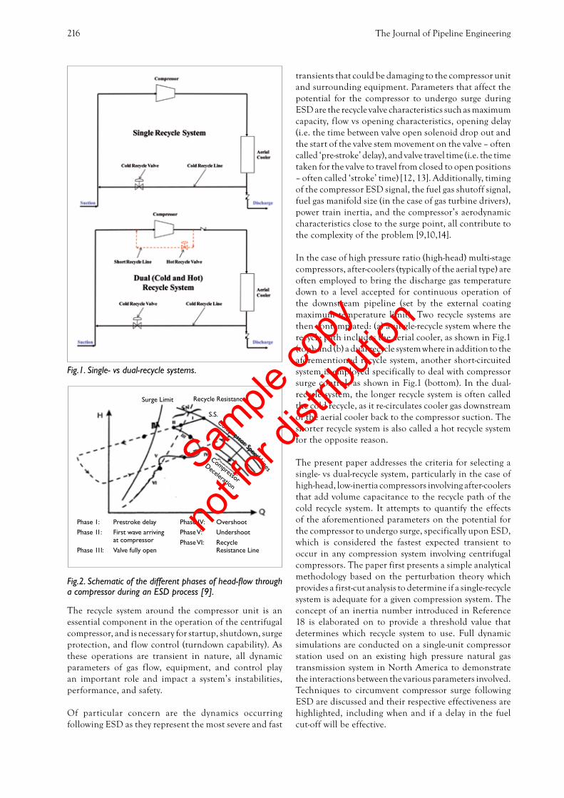
The Journal of Pipeline Engineering216
The recycle system around the compressor unit is an essential component in the operation of the centrifugal compressor, and is necessary for startup, shutdown, surge protection, and flow control (turndown capability). As these operations are transient in nature, all dynamic parameters of gas flow, equipment, and control play an important role and impact a system’s instabilities, performance, and safety.
Of particular concern are the dynamics occurring following ESD as they represent the most severe and fast
transients that could be damaging to the compressor unit and surrounding equipment. Parameters that affect the potential for the compressor to undergo surge during ESD are the recycle valve characteristics such as maximum capacity, flow vs opening characteristics, opening delay (i.e. the time between valve open solenoid drop out and the start of the valve stem movement on the valve – often called ‘pre-stroke’ delay), and valve travel time (i.e. the time taken for the valve to travel from closed to open positions – often called ‘stroke’ time) [12, 13]. Additionally, timing of the compressor ESD signal, the fuel gas shutoff signal, fuel gas manifold size (in the case of gas turbine drivers), power train inertia, and the compressor’s aerodynamic characteristics close to the surge point, all contribute to the complexity of the problem [9,10,14].
In the case of high pressure ratio (high-head) multi-stage compressors, after-coolers (typically of the aerial type) are often employed to bring the discharge gas temperature down to a level accepted for continuous operation of the downstream pipeline (set by the external coating maximum temperature limit). Two recycle systems are then contemplated: (a) a single-recycle system where the recycle path includes the aerial cooler, as shown in Fig.1 (top); and (b) a dual-recycle system where in addition to the aforementioned recycle system, another short-circuited system is employed specifically to deal with compressor surge control, as shown in Fig.1 (bottom). In the dual-recycle system, the longer recycle system is often called the cold recycle, as it re-circulates cooler gas downstream of the aerial cooler back to the compressor suction. The shorter recycle system is also called a hot recycle system for the opposite reason.
The present paper addresses the criteria for selecting a single- vs dual-recycle system, particularly in the case of high-head, low-inertia compressors involving after-coolers that add volume capacitance to the recycle path of the cold recycle system. It attempts to quantify the effects of the aforementioned parameters on the potential for the compressor to undergo surge, specifically upon ESD, which is considered the fastest expected transient to occur in any compression system involving centrifugal compressors. The paper first presents a simple analytical methodology based on the perturbation theory which provides a first-cut analysis to determine if a single-recycle system is adequate for a given compression system. The concept of an inertia number introduced in Reference 18 is elaborated on to provide a threshold value that determines which recycle system to use. Full dynamic simulations are conducted on a single-unit compressor station used on an existing high pressure natural gas transmission system in North America to demonstrate the interactions between the various parameters involved. Techniques to circumvent compressor surge following ESD are discussed and their respective effectiveness are highlighted, including when and if a delay in the fuel cut-off will be effective.
Fig.1. Single- vs dual-recycle systems.
Surge Limit
Phase 1: Prestroke delayPhase 11: First wave arriving at compressorPhase 111: Valve fully open
Phase IV: OvershootPhase V: UndershootPhase VI: Recycle Resistance Line
Recycle Resistance
S.S.Compressor Speed Lines
Compressor
Deceleration
Fig.2. Schematic of the different phases of head-flow through a compressor during an ESD process [9].
Sample
copy
not fo
r dist
ributi
on

4th Quarter, 2011 217
Description of an ESD processThe process of compressor station ESD is schematically depicted on a head-flow diagram in Fig.2, following a trend observed both experimentally and numerically [9-11]. Six phases are identified as the compressor decelerates from a steady-state point (S.S.) to zero flow and zero head across the compressor. Following an ESD, the operating point of the compressor follows approximately a straight line characterized by the slope (S) for a period of time before any expansion or pressure waves arrive at the compressor outlet or inlet, respectively, as a result of opening the recycle valve. This period corresponds to the recycle valve pre-opening (pre-stroke) delay, which is a combined effect of a process signal delay and inherent mechanical delay in opening of the recycle valve once an ESD signal is issued. During this phase (Phase I), although the driver power is assumed to be completely shut-off, the compressor continues to rotate due to the combined inertia of its shaft, impeller, and driver. The compressor decelerates due to the head across it, windage, friction, etc., according to the balance of the following equation:
where:
Wdriver = driver powerIdriver = driver inertiaNdriver = driver speedIc = compressor inertiaNc = compressor speedt = time Ha = compressor adiabatic head m = gas mass flow rate through the compressorηa = compressor adiabatic efficiency ηm = mechanical efficiency
In Equn (1) it is assumed that the driver power was set to zero instantaneously at the instant of ESD. While this is correct for cases where electric motors are used as drivers, it is not absolutely correct for cases with gas turbine drivers. White and Kurz [14] have shown that one of the key problems is that there is residual power from the gas turbine even after the fuel is shut off. This is due to two effects: one is that there is always some fuel gas remaining in the fuel gas manifold system which will continue to feed the gas turbine combustor and hence sustain power for a few hundred milliseconds; and secondly, the rotor inertia of the gas generator itself will continue to provide hot gas to the power turbine even at a decreasing temperature. These effects can be mathematically represented by describing the power term on the left hand side of Equn (1) as a declining function of time instead of setting it to zero at the instant of ESD. Similar treatment can be adopted to steam turbine drivers.
Once the recycle valve opens, a pressure wave travels downstream of the valve along the low-pressure part of
the recycle line and along the main suction line, while an expansion wave travels upstream of the valve along the high-pressure part of the recycle line and along the main discharge line. The first wave to arrive at the compressor suction or discharge sides depends on the distance, which either wave needs to travel, and the local speed of sound along the corresponding path. The time taken for either wave to arrive first to the compressor determines the duration of Phase II shown in Fig.2. Once this wave arrives at the compressor, the flow starts to increase through the compressor and the head decreases, and hence the beginning of Phase III. It can be shown that the slope (S) of the line identified in Fig.1 for Phases I and II can be expressed as [11]:
where:
A = pipe cross-section areaC1 = sound speed of the gas at suction conditionC2 = sound speed of the gas at discharge conditionHo = compressor head at steady-state pointk = isentropic exponent of the gasP1 = suction static pressureP2 = discharge static pressureR = gas constantT1 = suction gas temperatureZav = average gas compressibility factorρ1 = gas density at compressor inletζ = parameter defined as ZavRT1/ [( k - 1) / k]
The recycle valve continues to open to the maximum open position resulting in further pressure waves and expansion waves arriving at the compressor suction and discharge sides, respectively. However, due to gas inertia in the recycle line and mainline, the flow through the compressor tends to overshoot as is manifested by Phase IV, followed by a short period of undershoot (Phase V) around the recycle system resistance line shown in Fig.1. The final Phase VI is compressor wind-down in which small over- and under-shootings around the recycle resistance line occur until zero flow and zero head are reached.
Simple methodology to determine whether a single- or a dual-recycle system is required
The perturbation characteristic of Equn 2 represents the relationship between changes in the adiabatic head and actual inlet flow to the compressor for cases of no reflections from either ends to the compressor (i.e. the recycle valve is still closed and both suction and discharge lines are non-reflective). The maximum drop in the compressor speed during this period following an ESD and
Sample
copy
not fo
r dist
ributi
on

For more information visit www.clarion.org
As governments around the world search for answers to mitigate climate change through car-bon capture and storage, the pipeline industry will be meeting in Newcastle, UK, to develop the missing link: CO2 pipelines.
Forum programme
Over two days industry experts will meet to address the challenges presented by the transporta-tion of CO2 by pipeline including:
» The economics of pipeline transportation; » The materials to be used; » Regulations and risk assessment; » Hydraulic modelling; and, » Operations and maintenance.
Know where the pipeline market is heading – make sure you register for the In-ternational Forum on the Transportation of CO2 for CCS.
Join the industry in Newcastle, UK, to take the challenges of C02 transportation by pipeline head on.
19–21 June 2012Hilton Hotel, Newcastle, UK
ORGANIZERS
co2_fp-ad.indd 1 10/01/12 4:57 PM
Sample
copy
not fo
r dist
ributi
on

4th Quarter, 2011 219
before the compressor undergoes surge can be determined by running a tangent from the initial operating point with a slope S to the compressor characteristic at speed No - δNmax, as shown in Fig.3. If the compressor speed drops below this limiting speed during ESD operation (as a result of, for example, low compressor shaft inertia, an initial condition of high head, a late arrival of the first expansion wave to the compressor discharge or the pressure wave to the suction of the compressor due to opening of the recycle valve), the compressor will undergo reverse flow (surge). This is because the compressor impeller at this speed cannot sustain a positive flow against the prevailing high differential pressure (head) across it. In this case, the high differential pressure will drive reverse flow through the impeller while it is spinning forward, which is defined by the intersection of the characteristic line with the full compressor characteristic at the prevailing speed at this instant (point B in Fig.3), hence the first surge cycle. In summary:
if δN > δNmax surge will occur, andif δN < δNmax surge will not occur.
Here, δN is determined from ESD equation (1), which can be simplified for the case of gas turbine driven compressors as follows:
Theoretically, if the characteristic slope S is known, and the initial condition of the compressor (point ‘o’) is known, the maximum speed drop can be determined from geometric algebra established by Fig. 3 and the fan laws of the compressor characteristics, including the cubic representation of the full compressor characteristics to the left of the surge point [17]. One approximation is to assume that (No - δNmax) corresponds to the mainline characteristics line meeting the compressor speed line at the surge point (s) at speed = No - δNmax instead of being tangent to it at point (t) as shown in Fig.3. This approximation is, in fact, more realistic as the surge point (s) defines the surge limit. Following the fan laws the relation between adiabatic heads, actual inlet flows and compressor speeds at surge points can be correlated as follows:
According to the above discussion and referring to Fig.3, the following relation can be written:
where ‘S’ is the slope of the characteristic line defined by Equn 2.
Actual Inlet Flow
Fig.3. Determination of maximum drop in compressor speed before compressor surging following ESD.
For more information visit www.clarion.org
As governments around the world search for answers to mitigate climate change through car-bon capture and storage, the pipeline industry will be meeting in Newcastle, UK, to develop the missing link: CO2 pipelines.
Forum programme
Over two days industry experts will meet to address the challenges presented by the transporta-tion of CO2 by pipeline including:
» The economics of pipeline transportation; » The materials to be used; » Regulations and risk assessment; » Hydraulic modelling; and, » Operations and maintenance.
Know where the pipeline market is heading – make sure you register for the In-ternational Forum on the Transportation of CO2 for CCS.
Join the industry in Newcastle, UK, to take the challenges of C02 transportation by pipeline head on.
19–21 June 2012Hilton Hotel, Newcastle, UK
ORGANIZERS
co2_fp-ad.indd 1 10/01/12 4:57 PM
Sample
copy
not fo
r dist
ributi
on

The Journal of Pipeline Engineering220
Introducing Equn 2 into Equn 5, the following equations can be developed:
and finally,
Now combining Equns 7 and 3 and integrating, we arrive at the simple equation that determines the maximum (longest) time that the compressor can withstand before going into surge, i.e. before the arrival of the relief expansion or pressure waves resulting from opening the recycle valve, as follows:
Eequation 8, though simple and easy to evaluate, is significant. The value of δtmax thus calculated by this equation can be compared to the time it will take for the first relief expansion or pressure wave to arrive at the compressor discharge or suction side, respectively. This time of arrival
can be estimated from the sum of the recycle valve pre-stroke delay and the travel time of either the expansion or the pressure wave to arrive at the compressor. The latter is calculated from the distance along the corresponding piping between the recycle valve and the compressor and the local speed of sound in the gas, either on the discharge or the suction side, respectively.
Figure 4 shows an example of head-flow characteristics of a high-head, low-inertia compressor unit on a natural gas compression system depicted schematically in Fig.5. A steady-state operating point was assumed close to the surge control line as shown in the figure at Qo = 4.363m3/s and Ho = 37.072kJ/kg. Other relevant parameters required for the calculation of δtmax in Equn 8 are given in Table 1. The resulting δtmax is calculated as 116ms.
According to the axial distances along the suction and discharge piping separating the cold recycle valve from the compressor (see Fig.5), the arrival time of the expansion and pressure waves, along with valve pre-stroke delay are calculated in Table 2. These times are 296ms and 288ms, respectively. Clearly, the compressor in this case will undergo surge following an ESD operation since the time of arrival of either wave is much longer than δtmax of 116ms calculated above. In fact, the pre-stroke delay alone of this valve (= 200ms) is obviously too long to prevent the compressor unit from surging. The obvious solution is not only to employ a recycle valve that has a shorter pre-stroke delay, but to have it located very close to either compressor discharge
Inlet Flow (m3/s)
Fig.4. Example of high-head low-inertia compressor characteristics.
Sample
copy
not fo
r dist
ributi
on

4th Quarter, 2011 221
(preferable) or suction sides. This means, a dual-recycle system is required, i.e. the addition of a short (hot) recycle system as shown in Fig.5 (dotted line). Again, the function of the short recycle system is for ESD and surge protection, while the cold recycle system which includes the aerial cooler in the recycle path, is for unit startup and part-load operation.
If the compressor/power turbine combined inertia was 300kgm2 (instead of the 117kgm2), the time to surge would have been 297ms (rather than 116ms). Additionally, δtmax also depends on the initial operating point on the compressor characteristics (i.e. head and flow values) with respect to the surge line, as well as gas dynamic parameters involved in the equation, as mentioned earlier. The further the initial operating point from the surge line is, the longer the value of δtmax. This is due to the term (Qo - Qs) on the numerator of Equn 8. This will be discussed further below.
It should be emphasized that if the time to surge (δtmax) is longer than the combined pre-stroke delay time and the perturbation wave time, the compressor will not go into the first surge cycle. This does not mean that the compressor will be entirely surge free. The other important parameter that then comes to play is the piping capacitance (volume of gas) contained between the station check valve, the cold recycle valve and the compressor discharge side due to the presence of the aerial cooler and associated piping. This high-pressure gas volume needs to be relieved via the cold recycle valve to the lower pressure on the suction side. With the inclusion of the aerial cooler in the recycle path, the recycle valve size/capacity has to be large enough to relieve this pressure otherwise the compressor will surge, now due to this volume capacitance instead of the timing issues described earlier. This will be illustrated further below.
Therefore, it can be said that the above simple methodology applies to compression systems that do not involve large volume capacitance along the wave travelling path. The absence of a large volume capacitance system allows the perturbation wave to travel axially along the linear piping system without been dampened by a large capacitance that would act as a ‘muffler’ and substantially weaken its effects on the compressor.
Flow Conditions
Suction Pressure 8202 kPa-a
Suction Temperature 283 K
Discharge Pressure 11352 kPa-a
Discharge Temperature 314 K
Average Compressibility 0.817
Molecular weight 17.953 kg/kmol
Suction Density 76.560 kg/m3
Isentropic Exponent 1.482
Isentropic Efficiency 0.8
Mechanical Efficiency 0.96
Gas Constant 463.098 J/kg.K
C1 398.390 m/s
C2 436.7 m/s
Pipe Size (30" Nominal)
Internal Diameter 0.737 m
X-Sectional Area 0.426 m2
Operating Point
Qo 4.363 m3/s
Ho 37072 J/kg
Qs 3.482 m3/s
Hs 38863 J/kg
No 5500 RPM
575.959 rad/s
Inertia 117 kg.m2
Table 1. Example of compressor operating parameters.
Fig.5. Schematic of the example station layout showing the axial piping distance between the cold recycle valve and compressor suction and discharge sides of the compressor unit.
Valve Pre-stroke delay 200 ms
Discharge Piping Length 42 m
Expansion Wave Arrival Time 96.18 ms
Combined Time 296.18 ms
Suction Piping Length 35 m
Pressure Wave Arrival Time 87.85 ms
Combined Time 287.85 ms
Table 2. Calculation of arrival time of the expansion and pressure waves to compressor unit discharge and suction sides, respectively (cold recycle system).
Sample
copy
not fo
r dist
ributi
on

The Journal of Pipeline Engineering222
Inertia number Following numerous analyses conducted on different design philosophies of compression systems, and incorporating different types of centrifugal compressors, the decision to employ a short recycle system around the compressor unit to overcome the possibility of surging the unit during ESD operation lies in the balance between the following parameters:
• Effective compressor/driver rotor inertia defined at the compressor end, (I).
• The delay time before the recycle valve starts its opening stroke (that is the time associated with Phases I and II in the ESD process described above), (τ).
• The maximum fluid energy extracted from the compressor/driver power trains; and the compressor speed, which can be approximated by the product , where subscript (s) refers to conditions at the surge point at maximum compressor speed.
With the aid of Equn 8, a non-dimensional number can be derived that includes all of the above independent parameters. This dimensionless number, herein referred to as the inertia number (NI), is defined as:
A threshold value of the inertia number was found from actual installations and dynamic analyses conducted on 17 industrial compression systems employing different compressor models andstationdesign.Thisthresholdvaluewasfoundtobe≈30,
below which a shorter recycle system would definitely be needed to prevent the compressor unit from undergoing surge during ESD operation. When the inertia number is greater than 100, a single-recycle system would be adequate. For an inertia number in the range of 30-100, detailed dynamic simulation on the station should be conducted in a manner similar to the examples which will be presented in the next section. Table 3 gives the various operating and design parameters for the 17 industrial compression systems that were analysed and the respective inertia number, based on a value of τ corresponding to the cold recycle system. The comment column in Table 3 indicates whether the design incorporated a short (hot) recycle or not.
The above threshold value of the inertia number is useful for station design engineers, which allows a quick check to determine whether a short (hot) recycle system would be required for a type and model of compressor unit and the neighbouring equipment, particularly cooler and suction separators being in the recycle loop. If the calculation of the inertia number reveals a value less than or equal to 30, a shorter recycle system would be needed, and a detailed dynamic simulation should be conducted. If, on the other hand, the inertia number was approximately 100 or greater, a single-recycle system is acceptable, and a detailed dynamic simulation may not be required.
However, when a short (hot) recycle system is employed, often the compressor suction and discharge temperatures gradually climb during ESD, as warmer gas is recycled back to the suction of the compressor, which in turn increases the discharge temperature. Although throttling of the gas through
Table 3. Operating and design parameters to derive the inertia numbers for the various industrial compression systems analysed.
Station 1 (kg.m2) N (RPM) Flow (kg/s)
Hs (J/kg) !)ms* No of Stages
Cooler Inertia Number
Comment
1 36.1 6800 250 28000 200 1 No 13.08 Delay in Fuel Gas by 100 ms
2 33.7 8856 143 80600 200 2 Yes 12.62 Hot & Cold Recycle Installed
3 32.2 7780 125 64500 200 2 Yes 13.25 Hot & Cold Recycle Installed
4 56.5 6500 180 52000 200 2 Yes 13.98 Hot & Cold Recycle Installed
5 41.5 6671 150 40000 200 2 Yes 16.89 Hot & Cold Recycle Installed
6 243.6 6100 299 68772 200 2 Yes 24.17 Hot & Cold Recycle Installed
7 259.6 4250 380 26220 200 1 Yes 25.80 Hot & Cold Recycle Installed
8 116.8 6500 244 52625 200 2 Yes 21.07 Hot & Cold Recycle Installed
9 102.5 6000 35 160000 215 6 Yes 33.61 Hot & Cold Recycle Installed
10 113.5 6825 420 31000 588 1 Yes 7.57 Hot & Cold Recycle Installed
11 3.9 11967 3 117000 337 4 Yes 54.00 Hot & Cold Recycle Installed
12 6.1 11970 9 124386 324 4 Yes 27.61 Hot & Cold Recycle Installed
13 104.8 7850 51 160612 368 5 Yes 23.43 Hot & Cold Recycle Installed
14 94.3 8311 50 152825 368 6 Yes 25.30 Hot & Cold Recycle Installed
15 0.2 20000 20 32000 185 1 No 6.48 Hot Recycle
16 128.6 5194 480 32000 200 1 No 12.38 Hot Recycle
17 870.0 5775 350 39000 200 2 Yes 116.55 Only Cold Recycle
Sample
copy
not fo
r dist
ributi
on
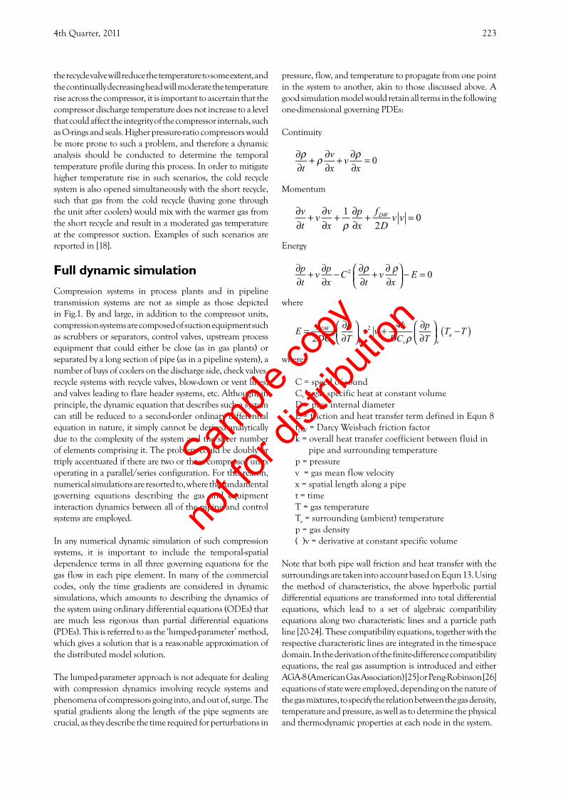
4th Quarter, 2011 223
the recycle valve will reduce the temperature to some extent, and the continually decreasing head will moderate the temperature rise across the compressor, it is important to ascertain that the compressor discharge temperature does not increase to a level that could affect the integrity of the compressor internals, such as O-rings and seals. Higher pressure-ratio compressors would be more prone to such a problem, and therefore a dynamic analysis should be conducted to determine the temporal temperature profile during this process. In order to mitigate higher temperature rise in such scenarios, the cold recycle system is also opened simultaneously with the short recycle, such that gas from the cold recycle (having gone through the unit after coolers) would mix with the warmer gas from the short recycle and result in a moderated gas temperature at the compressor suction. Examples of such scenarios are reported in [18].
Full dynamic simulation Compression systems in process plants and in pipeline transmission systems are not as simple as those depicted in Fig.1. By and large, in addition to the compressor units, compression systems are composed of suction equipment such as scrubbers or separators, control valves, upstream process equipment that could either be close (as in gas plants) or separated by a long section of pipe (as in a pipeline system), a number of bays of coolers on the discharge side, check valves, recycle systems with recycle valves, blow-down or vent lines, and valves leading to flare header systems, etc. Although, in principle, the dynamic equation that describes such a system can still be reduced to a second-order ordinary differential equation in nature, it simply cannot be derived analytically due to the complexity of the system and the sheer number of elements comprising it. The problem could be doubly or triply accentuated if there are two or three compressor units operating in a parallel/series configuration. For this reason, numerical simulations are resorted to, where the fundamental governing equations describing the gas and equipment interaction dynamics between all of the piping and control systems are employed.
In any numerical dynamic simulation of such compression systems, it is important to include the temporal-spatial dependence terms in all three governing equations for the gas flow in each pipe element. In many of the commercial codes, only the time gradients are considered in dynamic simulations, which amounts to describing the dynamics of the system using ordinary differential equations (ODEs) that are much less rigorous than partial differential equations (PDEs). This is referred to as the ‘lumped-parameter’ method, which gives a solution that is a reasonable approximation of the distributed model solution.
The lumped-parameter approach is not adequate for dealing with compression dynamics involving recycle systems and phenomena of compressors going into, and out of, surge. The spatial gradients along the length of the pipe segments are crucial, as they describe the time required for perturbations in
pressure, flow, and temperature to propagate from one point in the system to another, akin to those discussed above. A good simulation model would retain all terms in the following one-dimensional governing PDEs:
Continuity
Momentum
Energy
where
where:
C = speed of soundCv = gas specific heat at constant volumeD = pipe internal diameterE = friction and heat transfer term defined in Equn 8fDW = Darcy Weisbach friction factork = overall heat transfer coefficient between fluid in
pipe and surrounding temperaturep = pressurev = gas mean flow velocityx = spatial length along a pipe t = time T = gas temperatureTa = surrounding (ambient) temperaturep = gas density( )v = derivative at constant specific volume
Note that both pipe wall friction and heat transfer with the surroundings are taken into account based on Equn 13. Using the method of characteristics, the above hyperbolic partial differential equations are transformed into total differential equations, which lead to a set of algebraic compatibility equations along two characteristic lines and a particle path line [20-24]. These compatibility equations, together with the respective characteristic lines are integrated in the time-space domain. In the derivation of the finite-difference compatibility equations, the real gas assumption is introduced and either AGA-8 (American Gas Association) [25] or Peng-Robinson [26] equations of state were employed, depending on the nature of the gas mixtures, to specify the relation between the gas density, temperature and pressure, as well as to determine the physical and thermodynamic properties at each node in the system.
Sample
copy
not fo
r dist
ributi
on
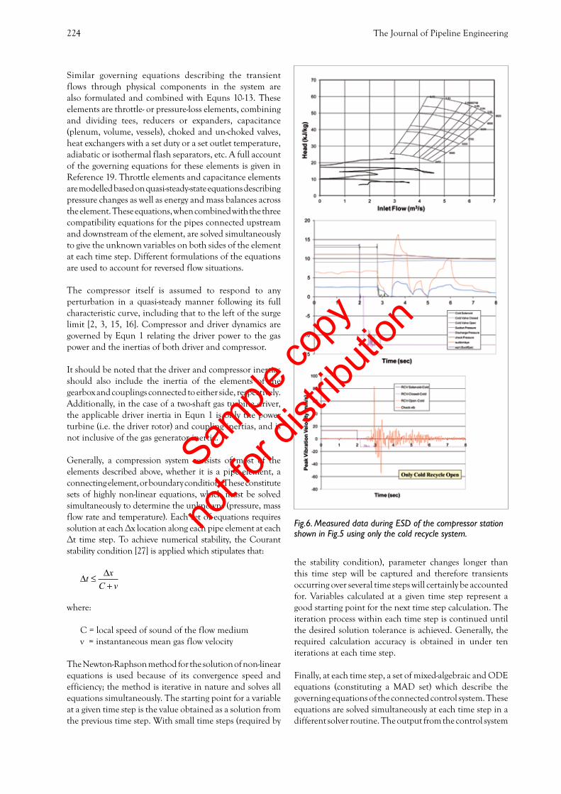
The Journal of Pipeline Engineering224
Similar governing equations describing the transient flows through physical components in the system are also formulated and combined with Equns 10-13. These elements are throttle- or pressure-loss elements, combining and dividing tees, reducers or expanders, capacitance (plenum, volume, vessels), choked and un-choked valves, heat exchangers with a set duty or a set outlet temperature, adiabatic or isothermal flash separators, etc. A full account of the governing equations for these elements is given in Reference 19. Throttle elements and capacitance elements are modelled based on quasi-steady-state equations describing pressure changes as well as energy and mass balances across the element. These equations, when combined with the three compatibility equations for the pipes connected upstream and downstream of the element, are solved simultaneously to give the unknown variables on both sides of the element at each time step. Different formulations of the equations are used to account for reversed flow situations.
The compressor itself is assumed to respond to any perturbation in a quasi-steady manner following its full characteristic curve, including that to the left of the surge limit [2, 3, 15, 16]. Compressor and driver dynamics are governed by Equn 1 relating the driver power to the gas power and the inertias of both driver and compressor.
It should be noted that the driver and compressor inertias should also include the inertia of the elements of the gearbox and couplings connected to either side, respectively. Additionally, in the case of a two-shaft gas turbine driver, the applicable driver inertia in Equn 1 is only the power turbine (i.e. the driver rotor) and coupling inertias, and is not inclusive of the gas generator inertia.
Generally, a compression system consists of most of the elements described above, whether it is a pipe element, a connecting element, or boundary condition. These constitute sets of highly non-linear equations, which must be solved simultaneously to determine the unknowns (pressure, mass flow rate and temperature). Each set of equations requires solutionateachΔxlocationalongeachpipeelementateachΔt time step.Toachievenumerical stability, theCourantstability condition [27] is applied which stipulates that:
where:
C = local speed of sound of the flow mediumv = instantaneous mean gas flow velocity
The Newton-Raphson method for the solution of non-linear equations is used because of its convergence speed and efficiency; the method is iterative in nature and solves all equations simultaneously. The starting point for a variable at a given time step is the value obtained as a solution from the previous time step. With small time steps (required by
the stability condition), parameter changes longer than this time step will be captured and therefore transients occurring over several time steps will certainly be accounted for. Variables calculated at a given time step represent a good starting point for the next time step calculation. The iteration process within each time step is continued until the desired solution tolerance is achieved. Generally, the required calculation accuracy is obtained in under ten iterations at each time step.
Finally, at each time step, a set of mixed-algebraic and ODE equations (constituting a MAD set) which describe the governing equations of the connected control system. These equations are solved simultaneously at each time step in a different solver routine. The output from the control system
Fig.6. Measured data during ESD of the compressor station shown in Fig.5 using only the cold recycle system.
Sample
copy
not fo
r dist
ributi
on
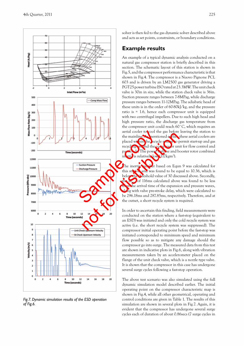
4th Quarter, 2011 225
solver is then fed to the gas dynamic solver described above and acts as set points, constraints, or boundary conditions.
Example results An example of a typical dynamic analysis conducted on a natural gas compressor station is briefly described in this section. The schematic layout of this station is shown in Fig.5, and the compressor performance characteristic is that shown in Fig.4. The compressor is a Nuovo Pignone PCL 603 and is driven by an LM2500 gas generator driving a PGT25 power turbine ISO rated at 23.3MW. The unit check valve is 30in in size, while the station check valve is 36in. Suction pressure ranges between 7-8MPag, while discharge pressure ranges between 11-12MPag. The adiabatic head of these units is in the order of 60-80kJ/kg, and the pressure ratio is ≈ 1.6, hence each compressor unit is equippedwith two centrifugal impellers. Due to such high head and high pressure ratio, the discharge gas temperature from thecompressorunitcouldreach60˚C,whichrequiresanaerial cooler to cool the gas before leaving the station to the mainline. As mentioned earlier, these aerial coolers are placed within the recycle system to permit start-up and gas recycling around the compressor unit for flow control and part loads. The power turbine and booster rotor combined inertia is relatively low (117kgm2).
The inertia number based on Equn 9 was calculated for this station and was found to be equal to 10.36, which is below the threshold value of 30 discussed above. Secondly, the δtmax of 116ms calculated above was found to be less than the arrival time of the expansion and pressure waves, along with valve pre-stroke delay, which were calculated to be 296.18ms and 287.85ms, respectively. Therefore, and at the outset, a short recycle system is required.
In order to ascertain this finding, field measurements were conducted on the station where a fast-stop (equivalent to an ESD) was initiated and only the cold recycle system was active (i.e. the short recycle system was suppressed). The compressor initial operating point before the fast-stop was initiated corresponded to minimum speed and minimum flow possible so as to mitigate any damage should the compressor go into surge. The measured data from this test are shown in indicative plots in Fig.6, along with vibration measurements taken by an accelerometer placed on the flange of the unit check valve, which is a nozzle type valve. It is shown that the compressor in this case has undergone several surge cycles following a fast-stop operation.
The above test scenario was also simulated using the full dynamic simulation model described earlier. The initial operating point on the compressor characteristic map is shown in Fig.4, while all other geometrical, operating and control conditions are given in Table 1. The results of this simulation are shown in several plots in Fig.7. Again, it is evident that the compressor has undergone several surge cycles each of duration of about 0.86secs (7 surge cycles in
Fig.7. Dynamic simulation results of the ESD operation of Fig.6.
Sample
copy
not fo
r dist
ributi
on

The Journal of Pipeline Engineering226
6secs). It is important to note that the station check valve closes immediately following the fast-stop, while the unit check valve is experiencing multiple cycles of opening and closing. The unit and station check valves are nozzle type valves with very little inherent damping. As indicated earlier, the obvious solution is not only to employ a recycle valve that has a shorter pre-stroke delay, but to locate it very close to either compressor discharge (preferable) or suction sides. This means the installation of a dual-recycle system, i.e. the addition of a short (hot) recycle system as shown in Fig.5 (dotted line). In fact this compressor has dual-recycle systems, which allowed another test similar to the previous one but with activation of both recycle systems: the cold and the hot ones. In this second test, higher compressor speed was permitted, and the initial condition before a fast-stop was initiated is that of Fig.4 and Table 1. The results of this test are shown in Fig.8. It appears that the compressor has undergone one mild surge (to the left of the surge line), though not fully to a deep surge characterized by a reverse flow through the unit. Following this one mild surge, the compressor is shown to have recovered to a normal shutdown scenario without subsequently going in and out of surge as in the previous test when only the cold recycle was activated.
This second test was also numerically simulated and the results are shown in Fig.9. It is indicated that the compressor has also gone one surge cycle initially although for a very short duration (about 0.2secs) unlike the first surge cycle in Fig.7 (which is approx. 1.3secs). The compressor is also shown to have recovered subsequently to a normal shutdown scenario without surging.
The question then arises as to why the compressor has undergone one mild (or short-lived) surge cycle even with both the hot and cold recycle systems activated.
In order to answer this question, it would be helpful to revert to the simple methodology described above as applied to the short (hot) recycle system. The hot recycle valve has a pre-stroke delay of 147ms, which despite being shorter than the cold recycle valve (which is 200ms) is still longer than when combined with the time of wave arrival calculated for the short recycle in Table 4. Recall that δtmax is calculated beforeforthisflowconditionisfoundtobe≈116ms.
Had the initial flow condition been slightly to the right on the flow characteristics map, δtmax would have been longer, and the compressor would not undergo any surge cycles following ESD or fast-stop. To demonstrate this, a dynamic simulation was carried out similar to the previous one but from an initial operating flow at 4.8m3/s (i.e. slightly to the right of the previous operating point of 4.363m3/s). For this new initial operating point, a similar calculation revealed that δtmax is 206ms, which is higher than the hot recycle pre-stroke delay plus the wave arrival time given in Table 4. Dynamic simulation was then conducted for this
Valve Pre-stroke delay 147 ms
Discharge Piping Length 6 m
Expansion Wave Arrival Time 13.74 ms
Combined Time 160.74 ms
Suction Piping Length 15 m
Pressure Wave Arrival Time 37.65 ms
Combined Time 184.65 ms
Table 4. Calculation of arrival time of the expansion and pressure waves to compressor unit discharge and suction sides, respectively (hot recycle system).
Fig.8. Measured data during ESD of the compressor station shown in Fig.5 using both hot and cold recycle systems.
Sample
copy
not fo
r dist
ributi
on
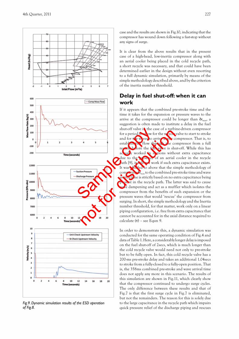
4th Quarter, 2011 227
case and the results are shown in Fig.10, indicating that the compressor has wound down following a fast-stop without any signs of surge.
It is clear from the above results that in the present case of a high-head, low-inertia compressor along with an aerial cooler being placed in the cold recycle path, a short recycle was necessary, and that could have been determined earlier in the design without even resorting to a full dynamic simulation, primarily by means of the simple methodology described above, and by the criterion of the inertia number threshold.
Delay in fuel shut-off: when it can workIf it appears that the combined pre-stroke time and the time it takes for the expansion or pressure waves to the arrive at the compressor could be longer than δtmax, a suggestion is often made to institute a delay in the fuel shut-off valve in the case of a turbine-driven compressor for a period to allow for the recycle valve to start to stroke and for the waves to arrive at the compressor. That is, to establish full flow through the compressor from a full recycle before the fuel valve is shut-off. While this has actually worked in stations without extra capacitance due to the presence of an aerial cooler in the recycle path [9], it will not work if such extra capacitance exists. It was alluded to above that the simple methodology of comparing δtmax to the combined pre-stroke time and wave arrival time is strictly based on no extra capacitance being present in the recycle path. The latter was said to cause wave dampening and act as a muffler which isolates the compressor from the benefits of such expansion or the pressure waves that would ‘rescue’ the compressor from surging. In short, the simple methodology and the Inertia number threshold, for that matter, work only on a linear piping configuration, i.e. free from extra capacitance that cannot be accounted for in the axial distance required to calculate (τ) – see Equn 9.
In order to demonstrate this, a dynamic simulation was conducted for the same operating condition of Fig.4 and data of Table 1. Here, a considerably longer delay is imposed on the fuel shut-off of 2secs, which is much longer than the cold recycle valve would need not only to pre-stroke but to be fully open. In fact, this cold recycle valve has a 200-ms pre-stroke delay and takes an additional 1.04secs to stroke from a fully-closed to a fully-open position. That is, the 358ms combined pre-stroke and wave arrival time does not apply any more in this scenario. The results of this simulation are shown in Fig.11, which clearly show that the compressor continued to undergo surge cycles. The only difference between these results and that of Fig.7 is that the first surge cycle in Fig.7 is eliminated, but not the remainders. The reason for this is solely due to the large capacitance in the recycle path which impairs quick pressure relief of the discharge piping and rescues
Fig.9. Dynamic simulation results of the ESD operation of Fig.8.
Sample
copy
not fo
r dist
ributi
on

SIGN UP TODAY FOR A FEE LISTING AT WWW.PIPELOOP.COM
Pipeloop is the global directory of pipeline professionals. Getting into the Pipeloop is the quickest and most effective way of promoting your presence, your skills, your product, your service in the pipeline sector.
Like other networking sites, users create an account and build a profi le outlining their skills as well as their experience. They can also search for other users using over 160 combinations of specialties and materials. The chief benefi t of Pipeloop is its unique focus on the pipeline sector.
Launched on Valentine’s Day this year, Pipeloop will bring the pipeline community together like never before.
So, if you’re looking for expert welding in Wyoming, want to sell inspection tools in India, need a recruiter in Rio, or might be hiring graduates in Gabon – it’s time you got in the Pipeloop, the global directory of pipeline professionals.
Pipeloop, brought to you by
Isn’t it time you were in the
FP_pipe_ad.indd 1 25/03/11 9:41 AM
Sample
copy
not fo
r dist
ributi
on

4th Quarter, 2011 229
the compressor from surging. In fact, such a large volume of gas at such high pressure would require a significantly large-capacity recycle valve to handle the relief flow. Such large capacity valves do not exist for a recycle size of 20in.
Concluding remarksThe old belief that “a single combined surge/recycle line is acceptable and is commonly used in the industry in the design of compressor stations” should be re-examined vigilantly. A simple methodology and an inertia number are introduced to help the designer of compression stations make the right decision as to whether a single- or a dual-recycle system is required for a given compression system and under given operating conditions.
It is also important to recognize the influence of salient parameters that play a key role in the dynamics of the recycle systems in compressor stations for all intended purposes and functions, namely: start-up, part loads, surge control, and surge protection following ESD or fast-stop. These very key parameters are:
1. compressor/power turbine rotor inertia;2. compressor pressure ratio (i.e. compressor adiabatic
head);3. volumetric capacitance of recycle system; 4. recycle system response time (i.e. recycle valve pre-
stroke delay, stroke time, time of arrival of expansion and pressure wave from the recycle valve to the compressor outlet and inlet, respectively);
5. compressor performance characteristics; and6. flow capacity of the recycle system.
The designer should always consider all of the above parameters and, with the aid of the methodology presented in this paper, as well as the aid of dynamic simulations, should be able to make the right decision in designing an adequate recycle system for the benefit of equipment integrity, performance and safety.
Fig.11. Results of dynamic simulation of an ESD operation using only the cold recycle system with 2secs delay in the fuel shut-off.
Fig.10. Results of dynamic simulation of an ESD operation from slightly higher initial flow conditions, and using both hot and cold recycle systems.
SIGN UP TODAY FOR A FEE LISTING AT WWW.PIPELOOP.COM
Pipeloop is the global directory of pipeline professionals. Getting into the Pipeloop is the quickest and most effective way of promoting your presence, your skills, your product, your service in the pipeline sector.
Like other networking sites, users create an account and build a profi le outlining their skills as well as their experience. They can also search for other users using over 160 combinations of specialties and materials. The chief benefi t of Pipeloop is its unique focus on the pipeline sector.
Launched on Valentine’s Day this year, Pipeloop will bring the pipeline community together like never before.
So, if you’re looking for expert welding in Wyoming, want to sell inspection tools in India, need a recruiter in Rio, or might be hiring graduates in Gabon – it’s time you got in the Pipeloop, the global directory of pipeline professionals.
Pipeloop, brought to you by
Isn’t it time you were in the
FP_pipe_ad.indd 1 25/03/11 9:41 AM
Sample
copy
not fo
r dist
ributi
on

The Journal of Pipeline Engineering230
References1. W.J.Turner and M.J.Simonson, 1985. Compressor
station transient flow modelled. Oil and Gas Journal, 79-83, May 20.
2. K.K.Botros, 1992. Transient phenomena in compressor stations during surge. 37th ASME International Gas Turbine and Aeroengine Congress and Exposition, Cologne, Germany, June 1 - 4, 1992; also appeared in the J. of Eng. for Gas Turbine and Power, 116, pp133-142, January.
3. K.K.Botros,P.J.Campbell, and D.B.Mah, 1991. Dynamic simulation of compressor station operation including centrifugal compressor and gas turbine. ASME Journal of Engineering for Gas Turbines and Power, 113, pp. 300-311, April, 1991.
4. K.M.Murphy et al., 1992. On modelling centrifugal compressors for robust control design. Int. Gas Turbine and Aeroengine Congress and Exposition, Cologne, Germany, 92-GT-231, June 1-4.
5. D.Paltovany and A.B.Focke, 1986. Predictive surge control optimization for a centrifugal compressor. J. of Turbomachinery, 108, 82- 89, July.
6. K.K.Botros, J.B.Jones, and O.Roorda, 1996. Flow characteristics and dynamics of swing check valves in compressible flow applications - Part I. ASME Pressure Vessels and Piping Conference, Symposium on Fluid Structure Interaction, Montreal, Quebec, Canada, PVP-Vol. 337, pp241-250, July 21-26.
7. E.B.Wylie, V.L.Streeter, and M.A.Stoner, 1974. Unsteady-state natural gas calculations in complex pipe systems. Society of Petroleum Engineering Journal, pp35- 43, Feb.
8. A.A.Al-Nahwi and M.B.Graf, 1997. Modeling of industrial pumping system dynamics. ASME Turbo-Expo Conference, Orlando, Florida, June 2-5.
9. K.K.Botros and D.J.Richards, 1995. Analysis of the effects of centrifugal compressor’s performance characteristics during ESD. 11th Symposium On Industrial Applications Of Gas Turbines, Canadian Gas Association, Banff, Alberta, Canada, October 11-13.
10. K.K.Botros, D.J .Richards, R.J .Brown, and D.M.Stachniak, 1993. Effects of low power turbine/compressor rotor inertia during shutdown. Presented at the 1993 Symposium on the Industrial Application of Gas Turbines, Canadian Gas Association, Banff, Alberta, October 13 - 15.
11. K.K.Botros, W.M.Jungowski, and D.J.Richards, 1996. Compressor station recycle system dynamics during emergency shutdown. ASME Transactions, J. Eng. for Gas Turbines and Power, 118, pp641-653, July.
12. K.K.Botros, B.J.Jones and D.J.Richards, 1996. Recycle dynamics during centrifugal compressor ESD, startup and surge control. International Pipeline Conference (IPC), ASME, Calgary, Alberta, Canada, June 9-14.
13. K.K.Botros, D.J.Richards, and O.Roorda, 1996. Effect of check valve dynamics on sizing of recycle systems for centrifugal compressors. 41st ASME International Gas Turbine And Aeroengine Congress And Exposition (Turbo-Expo), Birmingham, UK, June 10-13.
14. R.C.White and R.Kurz, 2006. Surge avoidance for compressor systems. Proceedings of the 35th Turbomachinery Symposium, George R. Brown Convention Center, Houston, Texas.
15. E.M.Greitzer, 1976. Surge and rotating stall in axial flow compressors. J. of Eng. for Power, Transaction of ASME, 190-198, April.
16. K.K.Moore and E.M.Greitzer, 1986. A theory of post stall transients in axial compression systems. J. of Eng. for Gas Turbines and Power, 108, 68-76.
17. K.K.Botros and G.Petela, 1994. Use of method of characteristics & quasi-steady approach in transient simulation of compressor stations. 1994 ASME Fluids Engineering Division Summer Meeting - Advances In Computational Methods in Fluid Dynamics, June 19 - 23, Lake Tahoe, Nevada, 196, pp325 - 338.
18. K.K.Botros and S.T.Ganesan, 2008. Dynamic instabilities in industrial compression systems with centrifugal compressors. Proceedings of the 37th Turbomachinery Symposium, George R. Brown Convention Center, Houston, Texas, September 8-11.
19. M.Mohitpour, K.K.Botros, and T.Van Hardeveld, 2008. Pipeline pumping and compression systems: a practical approach. Chapter 9, ASME Press.
20. M.J.Zucrow and J.P.Hoffman, 1976. Gas dynamics, Vol. I, and II, John Wiley & Sons Inc.
21. J.A.C.Kentfiled, 1993. Non-steady, one-dimensional, internal, compressible flows – theory and applications. Oxford Science Publication.
22. J.A.Fox, 1977. Hydraulic analysis of unsteady flow in pipe networks. John Wiley & Sons Inc.
23. A.Osiadacz, 1984. Simulation of transient gas flows in networks. Int. J. for Numerical Methods in Fluids, 4, pp13-24.
24. A.H.Shapiro, 1983. The dynamics and thermodynamics of compressible fluid flow – Vol. 2. E. Krieger Publishing Co., Malabar, Florida, pp972-973.
25. K.E.Starling and J.L.Savidge, 1992. Compressibility factors for natural gas and other related hydrocarbon gases. American Gas Association, Transmission Measurement Committee Report No. 8.
26. D.Y.Peng and D.B.Robinson, 1976. A new two-constant equation of state. Industrial and Engineering Chemistry: Fundamentals, 15, pp58-64, 1976.
27. R.Courant, K.Friedrichs, and H.Lewy, 1967. On the partial difference equations of mathematical physics. IBM Journal, March, pp215-234, English translation of the 1928 German original.
Sample
copy
not fo
r dist
ributi
on
4th Quarter, 2011 231
GRTgaz grid context
GRTgaz, the former transmission operator of Gaz de France, is an independent gas transmission operator
affiliated to GDF Suez. Its transmission network is 32,000 km in length, operated at an average pressure of 67 bar. A considerable number of action plans are dedicated to this network in order to maintain it at a high level of integrity as well as availability. As part of this, proactive surveys are performed, mainly by car and plane/helicopter: the average lengths covered in these ways are 170,000 km/year and 400,000 km/year, respectively, and each part of the network is visited approximately 18 times a year. Less than 10 failures per year related to third-party interference are recorded, mostly induced by undeclared excavation works. This is indeed a quite low failure rate compared to the length of the network; however the Ghislenghien incident is considered by the gas industry as a disaster reference, and any reasonable operator must always bear in mind that the likelihood of such an event cannot anymore be ignored.
As mentioned above, the average survey frequency is very significant (around 18 visits per year). The question that one
may ask is: on what basis is this survey frequency defined? Benchmarking of some transmission operators shows that the survey frequency is established on an historical basis combined with expert opinion reflecting a subjective empirical risk assessment.
Basic risk assumptionsThe goal of this paper is to deal with optimizing the survey frequency by means of a risk-assessment approach. Therefore, it is necessary to discuss some risk concepts which are of relevance here.
Risk is an empirical concept, both imprecise and subject to interpretation. Its aim is to measure, in the case of a specific industrial situation, the associated danger level. Commonly, as also mentioned in some standards [2], risk is defined as the combination of two components: the probability (or frequency) of an undesired hazardous event, and its consequence. This combination is expressed as:
In this analysis, our purpose is to reduce by as much as possible the risk of failure related to TPI, which mainly takes the form of undeclared excavation works. Therefore,
*Author’s contact details:tel: +33 1 4023 3750email: [email protected]
1. Failure means an unintentional release of gas (cf. [1])
by Samir Akel* and Frederic Riegert
GRTgaz, Paris, France
Buried gas pipelines are subject to failures1 related either to intrinsic defects, such as metal losses due to corrosion, or to extrinsic ones often induced by third-party interference (TPI). Feedback shows
that the latter is nowadays the main concern for gas system operators, since it represents over 50% of the overall recorded failures [1]. Those failures are sometimes accompanied by fatalities, serious injuries, and considerable damage such as at Ghislenghien in Belgium in 2004.
In order to improve pipeline integrity, pipeline operators try to select the main failure sources and put into operation preventive and/or corrective action plans to mitigate the associated danger. Action plans dedicated to TPI are decided at the early design stage of the pipeline by, for example, introducing an extra pipe wall thickness or installing concrete or steel slabs. At the operational stage, operators usually adopt proactive surveys by car or plane/helicopter, or even on foot, in order to detect suspicious excavation work, the main source of TPI damage. These action plans are considered as technical ones. Recently, action plans based on human or organizational factors were also defined. It is now acknowledged that both plans (technical and human/organizational) should be combined in order to obtain significant improvements in integrity.
The aim of the present paper is to deal with survey plans and, more precisely, how to optimize such plans in order to reduce by as much as possible the associated risk of failure.
Third-party interference: pipeline survey based on risk assessment
Sample
copy
not fo
r dist
ributi
on
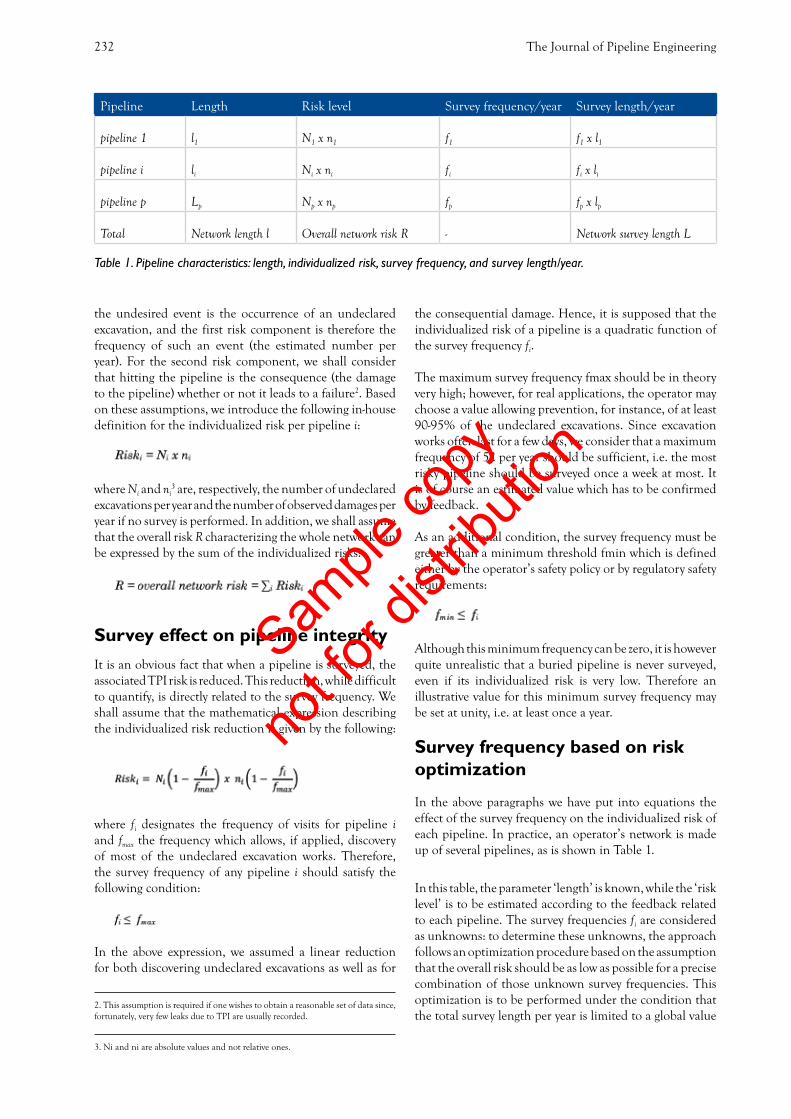
The Journal of Pipeline Engineering232
the undesired event is the occurrence of an undeclared excavation, and the first risk component is therefore the frequency of such an event (the estimated number per year). For the second risk component, we shall consider that hitting the pipeline is the consequence (the damage to the pipeline) whether or not it leads to a failure2. Based on these assumptions, we introduce the following in-house definition for the individualized risk per pipeline i:
where Ni and ni3 are, respectively, the number of undeclared
excavations per year and the number of observed damages per year if no survey is performed. In addition, we shall assume that the overall risk R characterizing the whole network can be expressed by the sum of the individualized risks:
Survey effect on pipeline integrityIt is an obvious fact that when a pipeline is surveyed, the associated TPI risk is reduced. This reduction, while difficult to quantify, is directly related to the survey frequency. We shall assume that the mathematical expression describing the individualized risk reduction is given by the following:
where fi designates the frequency of visits for pipeline i and fmax the frequency which allows, if applied, discovery of most of the undeclared excavation works. Therefore, the survey frequency of any pipeline i should satisfy the following condition:
In the above expression, we assumed a linear reduction for both discovering undeclared excavations as well as for
the consequential damage. Hence, it is supposed that the individualized risk of a pipeline is a quadratic function of the survey frequency fi.
The maximum survey frequency fmax should be in theory very high; however, for real applications, the operator may choose a value allowing prevention, for instance, of at least 90-95% of the undeclared excavations. Since excavation works often last for a few days, we consider that a maximum frequency of 52 per year should be sufficient, i.e. the most risky pipeline should be surveyed once a week at most. It is of course an estimated value which has to be confirmed by feedback.
As an additional condition, the survey frequency must be greater than a minimum threshold fmin which is defined either by the operator’s safety policy or by regulatory safety requirements:
Although this minimum frequency can be zero, it is however quite unrealistic that a buried pipeline is never surveyed, even if its individualized risk is very low. Therefore an illustrative value for this minimum survey frequency may be set at unity, i.e. at least once a year.
Survey frequency based on risk optimization
In the above paragraphs we have put into equations the effect of the survey frequency on the individualized risk of each pipeline. In practice, an operator’s network is made up of several pipelines, as is shown in Table 1.
In this table, the parameter ‘length’ is known, while the ‘risk level’ is to be estimated according to the feedback related to each pipeline. The survey frequencies fi are considered as unknowns: to determine these unknowns, the approach follows an optimization procedure based on the assumption that the overall risk should be as low as possible for a precise combination of those unknown survey frequencies. This optimization is to be performed under the condition that the total survey length per year is limited to a global value
2. This assumption is required if one wishes to obtain a reasonable set of data since, fortunately, very few leaks due to TPI are usually recorded.
3. Ni and ni are absolute values and not relative ones.
Pipeline Length Risk level Survey frequency/year Survey length/year
pipeline 1 l1 N1 x n1 f1 f1 x l1
pipeline i li Ni x ni fi fi x li
pipeline p Lp Np x np fp fp x lp
Total Network length l Overall network risk R - Network survey length L
Table 1. Pipeline characteristics: length, individualized risk, survey frequency, and survey length/year.
Sample
copy
not fo
r dist
ributi
on

4th Quarter, 2011 233
L: for illustration, in the GRTgaz’ case, L = 57,000km/year. This leads to:
The above condition reflects the fact that, for obvious economical reasons, there is an upper length limit in surveying the whole network; L designates this threshold which can be, for instance, established from the budget allocated to the survey action plan.
Solving the previous differential equation can be performed by means of the Lagrangian multiplier, and the solution is thus:
where :
Riskj = Nj x nj designates the individualized risk associatedto pipeline jlj is the length of pipeline jβ is a factor given by the following expression (in whichl designates the network length, i.e. l=∑li ):
β is always positive since:
The above condition4 indicates that for the total survey length per year L it is never sufficient to survey the total length of the network l at the maximum frequency fmax, otherwise there is no optimization procedure to perform.
As final remarks and according to the survey frequency expression, one may notice that:
• for two pipelines having the same absolute individualized risk level, the shorter one will have a higher survey frequency;
• for two pipelines having the same length, the riskier one will have a higher survey frequency;
• the survey frequency fi depends on relative values of the individualized risk level (the ratio Riskj / Riski) as shown below when developing the above survey frequency expression:
This characteristic hints that it is fairly useless to seek for high precision values for the absolute individualized risk per pipeline, since only risk ratios are relevant. Moreover, if absolute risk values are not available, it is still possible to give absolute risk levels based on an expert opinion (i.e. empirical risk classification for the network pipelines) in
4. Another logic condition that L must respect is L > fmin x l which, if not satisfied, means that the whole network cannot be surveyed at the minimum frequency fmin.
TPI 50%
mis hot-tapping5%
corrosion15%
other7%
groundmovement
7%
constructiondefect/material
failure16%
Fig.1. Failure causes for European transmission gas pipelines – source EGIG 2008 [1].
Sample
copy
not fo
r dist
ributi
on

The Journal of Pipeline Engineering234
anticipation that the risk ratios will mitigate the expert’s subjectivity and uncertainty.
Conditions consistency for survey frequencyAs mentioned above, the survey frequency must undergo the double condition:
Due to the fact that the factor β is always positive, then the optimized survey frequency fi is always less than fmax. Unfortunately, the other condition fi≥fmin is not always true; in fact fi may even be sometimes negative. In this case, the risk optimization should be mathematically performed under the constraint that the survey frequency fi must always be greater than fmin. Figure 2 shows how, in this case, optimization can be accomplished: it is an iterative procedure which can be easily introduced in a numerical tool.
Initial risk level evaluation for an a previously surveyed network
Most of pipeline operators already have their own survey plan based on historical survey frequencies. The overall risk, as well the individualized ones, are at a level which is undoubtedly lower than what it should be if the survey plan was not in place. In order to apply the proposed approach, one must restore the initial risk level (i.e. the
level of risk before applying the current empirical survey plan). Assuming that for a pipeline i, the current survey frequency is Fi
5 and the current individualized risk level is (N’i : n’i ), then the initial individualized risk level (Ni : ni ) can be estimated by:
ExampleFor an illustration, this approach was applied to GRTgaz’ network (for which l = 32,000km). Since hundreds of pipelines are involved, it was decided to gather them into 20 categories (i.e. p = 20), each category being characterized by the same individualized risk level. Figures 3 and 4 show the influence of the minimum frequency fmin if increased from once to four times a year. It can be seen that for ‘risky’ pipelines (categories 13 to 20), the survey frequencies remain unchanged in both cases.
Final commentsFigure 5 schematically summarizes the whole procedure described above. Situation A indicates the initial overall risk level if the network is not submitted to a survey plan; situation B reflects the current position: a lower risk level associated with a survey plan of an equivalent covered length L.
Fig.2. Process diagram showing the iterative procedure for a numerical estimation of survey frequencies.
5. fi designating the risk optimized survey frequency according to the present approach.
Sample
copy
not fo
r dist
ributi
on

4th Quarter, 2011 235
fmax 52/yr
fmin 1/yr
L 570,000km/yr
[Ni] [ni] li (km) fi
cat 1 0.001 1 446 1
cat 2 0.3 1 1,508 1
cat 3 0.5 3 2,321 1
cat 4 0.7 4 2,708 1
cat 5 0.9 1 1,802 1
cat 6 1.0 2 1,734 1
cat 7 1.2 5 2,061 1
cat 8 1.5 1 2,554 1
cat 9 1.8 1 1,807 1
cat 10 2.0 1 1,489 1
cat 11 2.5 14 2,377 26
cat 12 3.0 5 1,565 9
cat 13 3.5 11 1,456 38
cat 14 4.0 17 1,152 46
cat 15 5.0 10 1,527 41
cat 16 7.0 14 1,913 45
cat 17 10.0 61 1,484 51
cat 18 20.0 56 1,679 51
cat 19 40.0 73 814 52
cat 20 70.0 969 287 52
l = 32,000 km
fmax 52/yr
fmin 1/yr
L 570,000km/yr
[Ni] [ni] li (km) fi
cat 1 0.001 1 446 4
cat 2 0..3 1 1,508 4
cat 3 0.5 3 2,321 4
cat 4 0.7 4 2,708 4
cat 5 0.9 1 1,802 4
cat 6 1.0 2 1,734 4
cat 7 1.2 5 2,061 4
cat 8 1.5 1 2,554 4
cat 9 1.8 1 1,807 4
cat 10 2.0 1 1,489 4
cat 11 2.5 14 2,377 17
cat 12 3.0 5 1,565 4
cat 13 3.5 11 1,456 32
cat 14 4.0 17 1,152 43
cat 15 5.0 10 1,527 36
cat 16 7.0 14 1,913 42
cat 17 10.0 61 1,484 51
cat 18 20.0 56 1,679 51
cat 19 40.0 73 814 52
cat 20 70.0 969 287 52
l = 32,000 km
Ove
rall
netw
ork
risk
L (x 1 000 km)
Fig.3. Numerical simulation for fmin = one survey visit per year. Note that Ni and ni are standardized values for undeclared excavation frequency and observed damage, respectively.
Fig.4. Numerical simulation for fmin = four survey visits per year.
Fig.5. Schematic summary of survey optimization based on risk assessment.
Sample
copy
not fo
r dist
ributi
on
The Journal of Pipeline Engineering236
The proposed approach offers two alternatives:
• The risk level is presumed satisfactory: therefore one can theoretically optimize the survey resources (covered length) by maintaining the same level of the overall risk. This option leads to the situation D where the covered survey length is reduced (as well as the corresponding operational expenses), without any impact on the risk level. This can be obtained by defining a new combination of survey frequencies fi using the present approach,
• The risk level needs to be much more reduced with the same level of the allocated resources (i.e. same length L or the same operational expenses). This option leads to situation C which can be reached by means of a new combination of survey frequencies fi also established from the proposed approach. This second option is of course more appropriate, since it is consistent with the ultimate purpose of zero risk.
ConclusionA considerable number of technical action plans targeting network integrity are deployed nowadays by all pipeline operators. Measuring their effectiveness remains a challenge. Nevertheless, it is acknowledged that a zero risk level can never be reached (the ALARP principle and
Reference 3) unless unreasonable budgets are available, which the industry cannot afford. However, it is still possible to keep this situation as an ultimate target, at least by continuously improving existing action plans. In addition, it may be relevant that new action plans relating to new technologies (that may still to be discovered) may provide new margins of improvement based on the optimization of existing plans. Such improvements need to be made with no additional resources, i.e. it is necessary to do better with the same allocated operational expenses. The approach proposed here may be considered as a cost-effective way of following such a trend; in any case, it is wise to assume this approach as a tool to help the decision-making. It certainly gives an objective frame for a technical reference but an expert’s opinion, even if subjective, should always have the last word.
References1. European Gas Incident Data Group, 2008. Gas pipeline
incidents. 7th report, doc. no. EGIG 08.TV-B.0502, December.
2. FD ISO, 2009. Risk management. Guide 73, X 50-251, December.
3. French Safety Code, 2006. Transmission pipelines of flammable gases, liquid, or liquefied hydrocarbons and chemical products. August.
Sample
copy
not fo
r dist
ributi
on
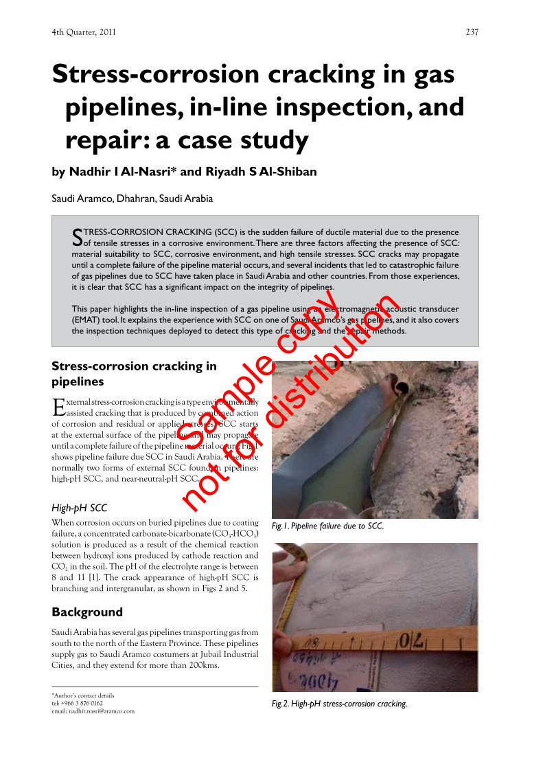
4th Quarter, 2011 237
Stress-corrosion cracking in pipelines
External stress-corrosion cracking is a type environmentally assisted cracking that is produced by combined action
of corrosion and residual or applied stresses. SCC starts at the external surface of the pipeline and may propagate until a complete failure of the pipeline material occurs; Fig.1 shows pipeline failure due SCC in Saudi Arabia. There are normally two forms of external SCC found in pipelines: high-pH SCC, and near-neutral-pH SCC.
High-pH SCCWhen corrosion occurs on buried pipelines due to coating failure, a concentrated carbonate-bicarbonate (CO3-HCO3) solution is produced as a result of the chemical reaction between hydroxyl ions produced by cathode reaction and CO2 in the soil. The pH of the electrolyte range is between 8 and 11 [1]. The crack appearance of high-pH SCC is branching and intergranular, as shown in Figs 2 and 5.
BackgroundSaudi Arabia has several gas pipelines transporting gas from south to the north of the Eastern Province. These pipelines supply gas to Saudi Aramco costumers at Jubail Industrial Cities, and they extend for more than 200kms.
by Nadhir I Al-Nasri* and Riyadh S Al-Shiban
Saudi Aramco, Dhahran, Saudi Arabia
STRESS-CORROSION CRACKING (SCC) is the sudden failure of ductile material due to the presence of tensile stresses in a corrosive environment. There are three factors affecting the presence of SCC:
material suitability to SCC, corrosive environment, and high tensile stresses. SCC cracks may propagate until a complete failure of the pipeline material occurs, and several incidents that led to catastrophic failure of gas pipelines due to SCC have taken place in Saudi Arabia and other countries. From those experiences, it is clear that SCC has a significant impact on the integrity of pipelines.
This paper highlights the in-line inspection of a gas pipeline using an electromagnetic acoustic transducer (EMAT) tool. It explains the experience with SCC on one of Saudi Aramco’s gas pipelines, and it also covers the inspection techniques deployed to detect this type of cracking and the repair methods.
Stress-corrosion cracking in gas pipelines, in-line inspection, and repair: a case study
*Author’s contact detailstel: +966 3 876 0162email: [email protected]
Fig.1. Pipeline failure due to SCC.
Fig.2. High-pH stress-corrosion cracking.
Sample
copy
not fo
r dist
ributi
on
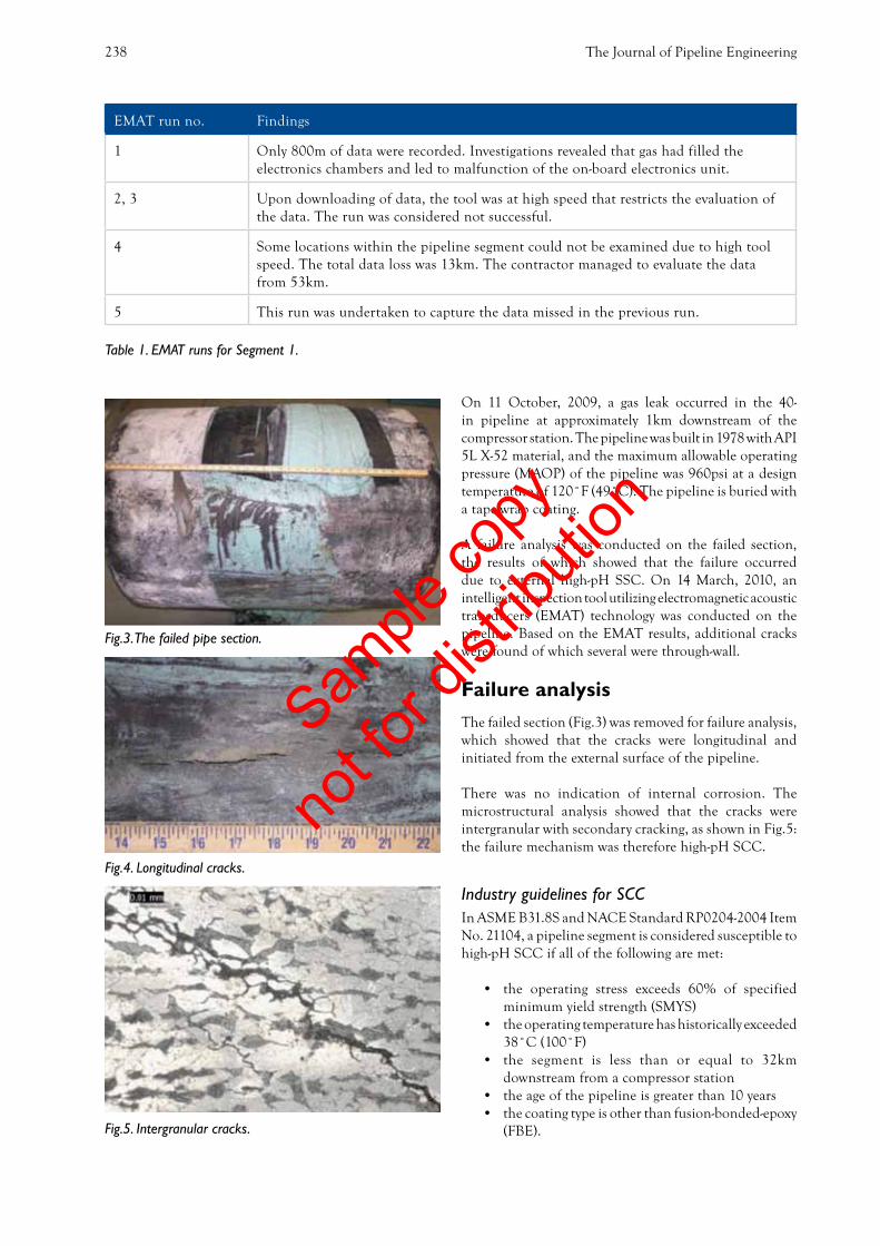
The Journal of Pipeline Engineering238
On 11 October, 2009, a gas leak occurred in the 40-in pipeline at approximately 1km downstream of the compressor station. The pipeline was built in 1978 with API 5L X-52 material, and the maximum allowable operating pressure (MAOP) of the pipeline was 960psi at a design temperatureof120˚F(49˚C).Thepipelineisburiedwitha tape-wrap coating.
A failure analysis was conducted on the failed section, the results of which showed that the failure occurred due to external high-pH SSC. On 14 March, 2010, an intelligent inspection tool utilizing electromagnetic acoustic transducers (EMAT) technology was conducted on the pipeline. Based on the EMAT results, additional cracks were found of which several were through-wall.
Failure analysis The failed section (Fig.3) was removed for failure analysis, which showed that the cracks were longitudinal and initiated from the external surface of the pipeline.
There was no indication of internal corrosion. The microstructural analysis showed that the cracks were intergranular with secondary cracking, as shown in Fig.5: the failure mechanism was therefore high-pH SCC.
Industry guidelines for SCCIn ASME B31.8S and NACE Standard RP0204-2004 Item No. 21104, a pipeline segment is considered susceptible to high-pH SCC if all of the following are met:
• the operating stress exceeds 60% of specified minimum yield strength (SMYS)
• the operating temperature has historically exceeded 38˚C(100˚F)
• the segment is less than or equal to 32km downstream from a compressor station
• the age of the pipeline is greater than 10 years• the coating type is other than fusion-bonded-epoxy
(FBE).
EMAT run no. Findings
1 Only 800m of data were recorded. Investigations revealed that gas had filled the electronics chambers and led to malfunction of the on-board electronics unit.
2, 3 Upon downloading of data, the tool was at high speed that restricts the evaluation of the data. The run was considered not successful.
4 Some locations within the pipeline segment could not be examined due to high tool speed. The total data loss was 13km. The contractor managed to evaluate the data from 53km.
5 This run was undertaken to capture the data missed in the previous run.
Table 1. EMAT runs for Segment 1.
Fig.3. The failed pipe section.
Fig.4. Longitudinal cracks.
Fig.5. Intergranular cracks.
Sample
copy
not fo
r dist
ributi
on

4th Quarter, 2011 239
ILI using an EMAT toolThe electromagnetic acoustic transducer (EMAT) tool was deployed as an inspection technique to detect SCC. The tool uses electromagnetic forces to induce ultrasonic waves into the pipe; the waves reflected by the pipe induce a varying electric current in the receiver, and this current signal is interpreted by software to provide indications about the internal structure of the pipe. This technology was used to inspect the first and the second segment of the 40-in pipeline, and was first used to examine the first pipeline segment downstream of the compressors station. Since it is the first time that this technology had been used by Saudi Aramco, several EMAT runs were conducted on the 66-km long segment to collect the entire data. Table 1 summarizes the findings for the EMAT runs for the first pipeline segment.
Unlike Segment 1, only one ILI using the EMAT tool was conducted for Segment 2. The pipeline diameter in this segment is 42in, and it is 62km in length.
Although the EMAT tool is not very different from a normal ILI tool, there were a couple of cases where it had got stuck in the pipelines: the tools were retrieved by cutting-out the
pipeline sections. The stuck tool locations were identified by the high electronic noise and the strong magnets on board the tools, and their exact positions were found by using metal powder on the pipeline surface at the selected locations. The metal powder indicated the locations of the two sections of the EMAT tool, as shown in Fig.6.
Inspection findings After analyzing the data from the EMAT tool for both segments, field verification took place by excavating the selected locations indicated by the tool. Table 2 summarizes the findings of both the EMAT tool and the field verifications. Figure 7 shows leaking SCC at Km 0.91.
During the field verifications of the locations indicated by the EMAT tool, the following were observed:
• SCC occurred underneath locations where the coating system (tape wrap) had failed. This led the pipeline to be exposed to the surrounding environment and become vulnerable to corrosion. Inadequate coating is a major contributor to the SCC of this buried pipeline.
Location EMAT indication
Field NDT finding
Km 0.91 N/A Scattered open cracks
Km 1.12
Km 1.21
Km 1.39 Linear 10 cracks; max. depth: 49%
Km 3.63 Linear Scattered cracks; max. depth: 42%
Km 4.12 Linear Scattered cracks; max. depth: 54%
Km 5.74 Linear Scattered cracks; max. depth: 31%
Km 7.67 Linear Scattered open cracks
Km 7.69 Linear Scattered cracks; max. depth: 52%
Km 43 Linear One crack; max. depth: 34%
Km 49.05 Linear Scattered cracks; max. depth: 38%
Km 76.10 Linear Scattered colonies; max. depth: 55%
Km 83.14 Linear Scattered colonies; max. depth: 58.5%
Km 102.3 Linear 4 cracks; max. depth: 17.5%
Table 2. Inspection results.
Fig.6. EMAT tool location.
Fig.7. Leaking SCC defect.
Sample
copy
not fo
r dist
ributi
on

The Journal of Pipeline Engineering240
• Some SCC colonies were found in associating with surface metal loss.
• Some SCC colonies were considered shallow (less than 10% of the pipe wall).
Most of the criteria stated in ASME B31.8S and NACE Standard RP0204-2004 for SCC were met for the segment that is less than 32km from the compressor station. However, there were some locations identified as having SCC defects which were beyond the distance specified in the guidelines (32km). Moreover, the stress level was 50-60%, which is below the industry guidelines.
Repair of SCC defectsOperating the pipeline at its design/operating conditions might cause additional cracks that could lead to leaks and/or rupture of the pipeline. According to the pipeline data, failure analysis, and inspection reports, the pipeline was considered susceptible to high-pH SCC. In order to determine the required repairs, the cracks were classified into three categories, based on their depth and length:
• deep cracks ( more than 60% of the wall thickness)• intermediate cracks (20% to 60% of the wall
thickness)• shallow cracks (less than 20% of the wall thickness)
Repair criteria were developed for each affected section based on field examinations and based on the defect mapping, the section was either replaced or repaired. Two types of repair were used before hydrotesting the pipeline to 110% SMYS. Shallow cracks were ground, while other cracks were encased in pressure-containing repair sleeves. Crack arresters were installed on the repaired section to ensure no propagation of the cracks during subsequent pipeline operations.
ConclusionThe gas pipeline with tape wrap coating was found susceptible to SCC. The first segment of the pipeline has the most SCC defects compared to the other segments, and this is in-line with the code and NACE guidelines. However, SCC defects were found at 50-60% SMYS. SCC defects were also found in the gas pipeline at 120km downstream of the compressor station.
The EMAT tool was found reliably to detect SCC, based on the verifications digs. Special considerations needed to be taken when running the tool.
SCC defects can be repaired by installing pressure-containing sleeve with crack arrestors. However, this should be based on the assessment of the cracks.
AcknowledgmentThe authors would like to thank Saudi Aramco management for its support in publishing this paper; Rami Al-Moaikel from the Pipelines Instrument Scraping Unit for his effort in providing the EMAT detailed results for this pipeline; and Waleed Al-Otaibi from the Materials’ Engineering Unit for his effort in conducting the failure analysis.
References1. M.Elboujdaini and M.Shehata. Stress corrosion
cracking: a Canadian perspective for oil and gas pipelines.
2. CEPA, 1997. Stress corrosion cracking – Recommended Practices.
3. ASME, 2001. B31.8S: Managing system integrity of gas pipelines.
4. NACE, 2004. Standard RP0204-2004.Sam
ple co
py
not fo
r dist
ributi
on

Editorial: continued from page 191
Though smaller than NACE International or PRCI, the European Pipeline Research Group (EPRG), founded in 1972, is influential both in its eponymous geographical area and elsewhere. Its members represent over 100,000km of operating pipelines, and manufacturing capacity of over 2m tons/yr of high-strength steel pipe. Among the drivers for its collaborative research programmes are the problems of the ageing network, the increasing costs of operations and maintenance, and the high cost of new connections. Representatives of EPRG, PRCI, and of the Australian Pipeline Industry Association (APIA) meet at biennial Joint Technical Meetings (in May, the 18th meeting was held in San Francisco) to present and discuss their research and promote joint projects. Together with DNV, EPRG is supporting a European-funded project on the safety of CO2-transmission pipelines, which was launched in July.
Probably one of the most important outcomes from this meeting was an acknowledgement that research that was kept confidential for too long was essentially wasted re-search. Although research has to be funded, and the current model in many countries was that industry has voluntarily to provide this funding (Brazil and China are examples of a different approach), it is clear that the results must be made public as soon as reasonable. A two-year morato-rium, to allow the funding companies to have some of the technological rewards from their investments, was seen as acceptable; longer delays in publicizing the results that could benefit the whole of the industry were not. DNV’s initiatives in making the details of the JIPs with which it is involved openly available through its website, and PRCI’s determination to promote partnerships with stakeholders, industry, and regulators, are good examples of where atti-tudes are leading in this regard. The spirit of this meeting was wholeheartedly in support.
The members of the Pipeline Committee, in alphabetic order of their company affiliations, are:
Colin McKinnon Chairman, JP KennyAsle Venås Secretary, DNVPatrick Rijneveld AllseasDavid Bruton Atkins BoreasNathalie Descusse BPJohn Lawson Chevron ETCMichael Krogh DongTheo Koeppe EuropipeAndrey Kalmykov GaspromPer-Atle Strømme GasscoElgar Kleijne HeeremaDouglas Souden HSE GSI Phillip Cooper IntecSeaAoki Masahiro JFE-steelJørgen Vestergård Sørensen MærskAndrew Palmer National University of SingaporeMarcello Jose Barbosa Teixeira PetrobrasKjell Arnfinsen PTILPulici Massimo SaipemMichiel Jansen ShellSvein Harald Såtendal StatoilT Sriskandarajah Subsea 7Martin Connelly Tata SteelSylvian Denniel TechnipFrederico Tintori TenarisStéphanie Le-Douaron TotalTanja Schmidt VM tubesNino Fogliani Woodside
Permanent DNV members:Leif Collberg DNVMorten Johnsrud DNVØyvin Eriksen DNVSam
ple co
py
not fo
r dist
ributi
on

Sample
copy
not fo
r dist
ributi
on