Embed Size (px)
Citation preview
University of Technology Sydney
Incorporating Prior Domain Knowledge into
Inductive Machine Learning
Its implementation in contemporary capital
markets
A dissertation submitted for the degree of
Doctor of Philosophy in Computing Sciences
by
Ting Yu
Sydney, Australia
2007

c© Copyright by
Ting Yu
2007

CERTIFICATE OF AUTHORSHIP/ORIGINALITY
I certify that the work in this thesis has not previously been submitted for a
degree nor has it been submitted as a part of requirements for a degree except as
fully acknowledged within the text.
I also certify that the thesis has been written by me. Any help that I have
received in my research work and the preparation of the thesis itself has been
acknowledged. In addition, I certify that all information sources and literature
used are indicated in the thesis.
Signature of Candidate
ii

Table of Contents
1 Introduction . . . . . . . . . . . . . . . . . . . . . . . . . . . . . . . . 1
1.1 Overview of Incorporating Prior Domain Knowledge into Inductive
Machine Learning . . . . . . . . . . . . . . . . . . . . . . . . . . . 2
1.2 Machine Learning and Prior Domain Knowledge . . . . . . . . . . 3
1.2.1 What is Machine Learning? . . . . . . . . . . . . . . . . . 3
1.2.2 What is prior domain knowledge? . . . . . . . . . . . . . . 6
1.3 Motivation: Why is Domain Knowledge needed to enhance Induc-
tive Machine Learning? . . . . . . . . . . . . . . . . . . . . . . . . 9
1.3.1 Open Areas . . . . . . . . . . . . . . . . . . . . . . . . . . 12
1.4 Proposal and Structure of the Thesis . . . . . . . . . . . . . . . . 13
2 Inductive Machine Learning and Prior Domain Knowledge . . 15
2.1 Overview of Inductive Machine Learning . . . . . . . . . . . . . . 15
2.1.1 Consistency and Inductive Bias . . . . . . . . . . . . . . . 17
2.2 Statistical Learning Theory Overview . . . . . . . . . . . . . . . . 22
2.2.1 Maximal Margin Hyperplane . . . . . . . . . . . . . . . . . 30
2.3 Linear Learning Machines and Kernel Methods . . . . . . . . . . 31
2.3.1 Support Vector Machines . . . . . . . . . . . . . . . . . . . 33
2.3.2 ε-insensitive Support Vector Regression . . . . . . . . . . . 37
2.4 Optimization . . . . . . . . . . . . . . . . . . . . . . . . . . . . . 38
2.5 Prior Domain Knowledge . . . . . . . . . . . . . . . . . . . . . . . 39
iii

2.5.1 Functional or Representational Form . . . . . . . . . . . . 42
2.5.2 Relatedness Between Tasks and Domain Knowledge . . . . 42
2.6 Summary . . . . . . . . . . . . . . . . . . . . . . . . . . . . . . . 46
3 Incorporating Prior Domain Knowledge into Inductive Machine
Learning . . . . . . . . . . . . . . . . . . . . . . . . . . . . . . . . . . . . 48
3.1 Overview of Incorporating Prior Domain Knowledge into Inductive
Machine Learning . . . . . . . . . . . . . . . . . . . . . . . . . . . 49
3.2 Consistency, Generalization and Convergence with Domain Knowl-
edge . . . . . . . . . . . . . . . . . . . . . . . . . . . . . . . . . . 52
3.2.1 Consistency with Domain Knowledge . . . . . . . . . . . . 52
3.2.2 Generalization with Domain Knowledge . . . . . . . . . . 54
3.2.3 Convergence with Domain Knowledge . . . . . . . . . . . . 58
3.2.4 Summary . . . . . . . . . . . . . . . . . . . . . . . . . . . 59
3.3 Using Prior Domain Knowledge to Preprocess Training Samples . 62
3.4 Using Prior Domain Knowledge to Initiate the Hypothesis Space
or the Hypothesis . . . . . . . . . . . . . . . . . . . . . . . . . . . 65
3.5 Using Prior Domain Knowledge to Alter the Search Objective . . 69
3.5.1 Learning with Constraints . . . . . . . . . . . . . . . . . . 70
3.5.2 Learning with Weighted Examples: . . . . . . . . . . . . . 76
3.5.3 Cost-sensitive Learning . . . . . . . . . . . . . . . . . . . . 77
3.6 Using Domain Knowledge to Augment Search . . . . . . . . . . . 78
3.7 Semi-parametric Models and Hierarchical Models . . . . . . . . . 79
iv

3.8 Incorporating Financial Domain Knowledge into Inductive Ma-
chine Learning in Capital Markets . . . . . . . . . . . . . . . . . . 82
3.9 Summary . . . . . . . . . . . . . . . . . . . . . . . . . . . . . . . 85
4 Methodology . . . . . . . . . . . . . . . . . . . . . . . . . . . . . . . 87
4.1 Semi-parametric Hierarchical Modelling . . . . . . . . . . . . . . . 88
4.1.1 Vector Quantization . . . . . . . . . . . . . . . . . . . . . 90
4.1.2 VQSVM and Semi-parametric Hierarchical Modelling . . . 92
4.1.3 Remarks of the Proposal Model . . . . . . . . . . . . . . . 94
4.2 A Kernel Based Feature Selection via Analysis of Relevance and
Redundancy . . . . . . . . . . . . . . . . . . . . . . . . . . . . . . 95
4.2.1 Feature Relevance and Feature Redundancy . . . . . . . . 96
4.2.2 Mutual Information Measurement . . . . . . . . . . . . . . 100
4.2.3 ML and MP Constraints . . . . . . . . . . . . . . . . . . . 102
4.2.4 Remarks of the Proposal Method . . . . . . . . . . . . . . 103
4.3 Rule base and Inductive Machine Learning . . . . . . . . . . . . . 103
5 Application I – Classifying Impacts from Unexpected News Events
to Stock Price Movements . . . . . . . . . . . . . . . . . . . . . . . . . 106
5.1 Introduction . . . . . . . . . . . . . . . . . . . . . . . . . . . . . . 106
5.2 Methodologies and System Design . . . . . . . . . . . . . . . . . . 109
5.3 Domain Knowledge Represented By Rule Bases . . . . . . . . . . 111
5.3.1 Domain Knowledge . . . . . . . . . . . . . . . . . . . . . . 111
v

5.3.2 Using Domain Knowledge to help the data-preparation of
Machine Learning . . . . . . . . . . . . . . . . . . . . . . . 112
5.3.3 Using Time Series Analysis to Discover Knowledge . . . . 115
5.4 Document Classification Using Support Vector Machine . . . . . . 117
5.5 Experiments . . . . . . . . . . . . . . . . . . . . . . . . . . . . . . 118
5.6 Summary . . . . . . . . . . . . . . . . . . . . . . . . . . . . . . . 120
6 Application II – Measuring Audit Quality . . . . . . . . . . . . . 121
6.1 VQSVM for Imbalanced Data . . . . . . . . . . . . . . . . . . . . 122
6.1.1 Algorithms . . . . . . . . . . . . . . . . . . . . . . . . . . 124
6.1.2 Experiments . . . . . . . . . . . . . . . . . . . . . . . . . . 128
6.1.3 Summary . . . . . . . . . . . . . . . . . . . . . . . . . . . 132
6.2 Feature Selections . . . . . . . . . . . . . . . . . . . . . . . . . . . 134
6.2.1 Algorithms . . . . . . . . . . . . . . . . . . . . . . . . . . 134
6.2.2 Experiments . . . . . . . . . . . . . . . . . . . . . . . . . . 137
6.2.3 Summary . . . . . . . . . . . . . . . . . . . . . . . . . . . 141
7 Conclusion and Future Works . . . . . . . . . . . . . . . . . . . . . 143
7.1 Brief Review and Contributions of this Thesis . . . . . . . . . . . 143
7.2 Future Research . . . . . . . . . . . . . . . . . . . . . . . . . . . . 145
A Abbreviation . . . . . . . . . . . . . . . . . . . . . . . . . . . . . . . 151
B Table of Symbols . . . . . . . . . . . . . . . . . . . . . . . . . . . . . 153
References . . . . . . . . . . . . . . . . . . . . . . . . . . . . . . . . . . . 154
vi

List of Figures
1.1 Inductive Machine Learning System by the General Learning Process 5
1.2 An Example of Inductive Machine Learning without and with Do-
main Knowledge . . . . . . . . . . . . . . . . . . . . . . . . . . . 11
1.3 Domain Knowledge and Inductive Machine Learning in the Given
Domain . . . . . . . . . . . . . . . . . . . . . . . . . . . . . . . . 12
2.1 More than one functions that fits exactly the data . . . . . . . . . 24
2.2 Risk, Empirical Risk vs. Function Class . . . . . . . . . . . . . . 25
2.3 Architecture of SV Machines . . . . . . . . . . . . . . . . . . . . . 34
3.1 A spectrum of learning tasks [Mit97b] . . . . . . . . . . . . . . . . 49
3.2 A set of hypothesis spaces . . . . . . . . . . . . . . . . . . . . . . 55
3.3 8-2-1 Artificial Neural Network . . . . . . . . . . . . . . . . . . . 56
3.4 Virtual Samples in SVM . . . . . . . . . . . . . . . . . . . . . . . 63
3.5 Kernel Jittering . . . . . . . . . . . . . . . . . . . . . . . . . . . . 67
3.6 Catalytic Hints . . . . . . . . . . . . . . . . . . . . . . . . . . . . 74
4.1 A Simple Example of Two-dimensional LBG-VQ [GG92] . . . . . 91
4.2 Hierarchical Modelling with SV Machines, which modifies the orig-
inal SVM (see figure 2.3) . . . . . . . . . . . . . . . . . . . . . . . 93
4.3 f1, f2 are relevant features, but the structures of influence are
different . . . . . . . . . . . . . . . . . . . . . . . . . . . . . . . . 98
4.4 The domain knowledge may be contained by the optimal set of
features (or approximated Markov Blanket) partially or entirely. . 103
vii

5.1 Structure of the classifier . . . . . . . . . . . . . . . . . . . . . . . 110
5.2 The half hourly Volume Weighted Average Prices and net-of-market
return sequences of AMP . . . . . . . . . . . . . . . . . . . . . . . 118
5.3 Shocks (large volatilities), Trend and Changing Points . . . . . . . 119
6.1 VQSVM in case of a linear separable data set . . . . . . . . . . . 125
6.2 In the audit data set, the observations (the bigger points) of the
minority class is scattered with those (the smaller darker points)
of the majority class . . . . . . . . . . . . . . . . . . . . . . . . . 129
6.3 The measurements in the FCBF algorithm proposed by Lei Yu and
Huan Liu [YL04] . . . . . . . . . . . . . . . . . . . . . . . . . . . 135
6.4 The test accuracy of models constructed by a SVR while eliminat-
ing one feature every iteration. The x-axis is the index of feature
in the ascending list, and the y-axis is the R-square. . . . . . . . . 137
6.5 The test accuracy of SVR models while eliminating one feature
every iteration. The x-axis is the index of feature in the ascending
list, and the y-axis is the value of R-square. . . . . . . . . . . . . 140
viii
List of Tables
1.1 An example of a data set . . . . . . . . . . . . . . . . . . . . . . . 5
2.1 A list of empirical risk and true risk functions . . . . . . . . . . . 19
3.1 Comparison of purely analytical and purely inductive learning [Mit97b] 50
6.1 Four UCI data sets and Audit data set with the numbers of local
models. . . . . . . . . . . . . . . . . . . . . . . . . . . . . . . . . 128
6.2 Test Results of the VQSVM . . . . . . . . . . . . . . . . . . . . . 131
6.3 The RBF SVM with the different values of sigma produces differ-
ent lists of ranked features. The lists are ordered from the least
important to the most important. . . . . . . . . . . . . . . . . . 138
ix

Acknowledgments
This research is supported by the Institute for Information and Communica-
tion Technologies (IICT), the e-Markets Research Program in the University of
Technology, Sydney, Capital Markets CRC Ltd., the International Institute of
Forecasters (IIF) and the SAS Institute.
I would like to thank my advisors Dr Tony Jan, A/Professor Simeon Simoff,
and Professor John Debenham in the Faculty of Information Technology and
Professor Donald Stokes in the School of Accounting for their efforts. I would
like to thank Dr Longbing Cao, Dr Maolin Huang, Professor Chengqi Zhang
and A/Professor Tom Hintz in the Faculty of Information Technology, Prof Mark
Tennant in the Graduate School, Dr Boris Choy, Dr Yakov Zinder, Dr Mark Crad-
dock, Professor Alexander Novikov, Dr Ronald M. Sorli and Dr Narelle Smith
in the Department of Mathematical Sciences, and A/Professor Patrick Wilson
and Professor Tony Hall in the School of Finance and Economics, University of
Technology, Sydney for their kind supports. I would like also to thank Deborah
Turnbull for her precise proof-reading.
I would like to also thank my colleagues, Dr Debbie Zhang, Paul Bogg and
other members in the e-Markets Research Group, my friends, Angie Ng and
Caesar Tsai, and numerous reviewers.
Final and most thanks to my parents, who support me with their love for all
my life.
Thank you.
Sydney, Australia, February 2007
x

Vita
2003 - 2007 Ph.D (Computing Science), The Faculty of Information Tech-
nology, The University of Technology, Sydney, Australia.
2001 - 2002 M.sc (Distributed Multimedia System), The School of Comput-
ing, The University of Leeds, Leeds, United Kingdom.
1993 - 1997 B.eng (Industrial Design), The College of Computer Science,
The Zhejiang University, Hangzhou, P.R. China.
Publications
Ting Yu, Simeon Simoff and Donald Stokes. Incorporating Prior Domain Knowl-
edge into a Kernel Based Feature Selection. The 11th Pacific-Asia Conference
on Knowledge Discovery and Data Mining (PAKDD 2007), Nanjing, P.R. China,
May 2007.
Ting Yu. Incorporating Prior Domain Knowledge into Inductive Machine Learn-
ing. Technique Report in the International Institute of Forecasters (IIF), The
University of Massachusetts, Amherst, USA, October 2006.
Ting Yu, Tony Jan, John Debenham and Simeon Simoff. Classify Unexpected
News Impacts to Stock Price by Incorporating Time Series Analysis into Support
Vector Machine. The 2006 International Joint Conference on Neural Networks
xi

(IJCNN 2006), 2006 IEEE World Congress on Computational Intelligence, 16-21
July, Vancouver, BC, Canada
Ting Yu, John Debenham, Tony Jan and Simeon Simoff, 2006, Combine Vector
Quantization and Support Vector Machine for Imbalanced Datasets, in Interna-
tional Federation Information Processing, Volume 217, Artificial Intelligence in
Theory and Practice, ed. M. Bramer, Boston: Springer, pp. 81-88.
Ting Yu, Tony Jan, John Debenham and Simeon Simoff. Incorporate Domain
Knowledge into Support Vector Machine to Classify Price Impacts of Unexpected
News. The Fourth Australasian Data Mining Conference, 5-6 December 2005,
Sydney, Australia 2004
Ting Yu, Tony Jan, John Debenham and Simeon Simoff. Incorporating Prior
Domain Knowledge in Machine Learning: A Review. 2004 International Confer-
ence on Advances in Intelligent Systems - Theory and Applications. November
2004, Luxembourg
Tony Jan, Ting Yu, John Debenham and Simeon Simoff. Financial Prediction us-
ing Modified Probabilistic Learning Network with Embedded Local Linear Mod-
els. CIMSA2004-IEEE International Conference on Computational Intelligence
for Measurement Systems and Applications, July 2004, Boston, MD, USA
Ting Yu and John Debenham. Using an Associate Agent to Improve Human-
Computer Collaboration in an E-Market System. WCC2004-AIAI,The Sympo-
sium on Professional Practice in AI, August 2004, Toulouse, France
xii

Ting Yu and Simeon J. Simoff. Plan Recognition as an Aid in Virtual Worlds.
Australian Workshop on Interactive Entertainment 2004,13th February 2004,
Sydney, Australia
xiii

Abstract
An ideal inductive machine learning algorithm produces a model best approx-
imating an underlying target function by using reasonable computational cost.
This requires the resultant model to be consistent with the training data, and
generalize well over the unseen data. Regular inductive machine learning algo-
rithms rely heavily on numerical data as well as general-purpose inductive bias.
However certain environments contain rich domain knowledge prior to the learn-
ing task, but it is not easy for regular inductive learning algorithms to utilize prior
domain knowledge. This thesis discusses and analyzes various methods of incor-
porating prior domain knowledge into inductive machine learning through three
key issues: consistency, generalization and convergence. Additionally three new
methods are proposed and tested over data sets collected from capital markets.
These methods utilize financial knowledge collected from various sources, such
as experts and research papers, to facilitate the learning process of kernel meth-
ods (emerging inductive learning algorithms). The test results are encouraging
and demonstrate that prior domain knowledge is valuable to inductive learning
machines.
xiv

CHAPTER 1
Introduction
As a major subfield of artificial intelligence, machine learning has gained a broader
attention in recent years. The Internet makes a variety of information more easily
accessible than ever before, creating strong demands for efficient and effective
methods to process large amounts of data in both industrial and scientific research
communities. The application of machine learning methods to large databases
is called Data Mining or Knowledge Discovery [Alp04]. Despite the existence of
hundreds of new machine learning algorithms, from a machine learning academic
researcher’s perspective, current research remains in preliminary status. If the
ultimate goal is to develop a machine that is capable of learning at the level of the
human mind, the journey has only just begun [Sil00]. This thesis is but one step
in that journey, and will focus on exploring the outstanding question: How can
a learning system represent and incorporate prior domain knowledge to facilitate
the process of learning?
This introductory chapter is divided into five sections: Section 1.1 provides
an overview of the research problem; Section 1.2 defines the concepts of inductive
machine learning and domain knowledge; Section 1.3 presents the motivation for
this dissertation; and Section 1.4 describes the approach that was undertaken,
providing an overview of the subsequent chapters and the structure of the docu-
ment.
1

1.1 Overview of Incorporating Prior Domain Knowledge
into Inductive Machine Learning
The majority of machine learning systems learn from scratch, inducing models
from a set of training examples without considering existing prior domain knowl-
edge. Consequently, most machine learning systems do not take advantage of
previously acquired domain knowledge when learning a new and potentially re-
lated task. Unlike human learners, these systems are not capable of accumulating
domain knowledge and sequentially improving their ability to learn tasks [Sil00].
The majority of research incorporating prior domain knowledge into inductive
machine learning has been done in the fields of pattern recognition and bioinfor-
matics (see chapter 3 in detail). Still, there is no adequate theory of how prior
domain knowledge can be retained and then selectively incorporated when learn-
ing a new task. Apart from pattern recognition and bioinformatics, a few similar
research projects have been done in computational finance, another prevailing
application of machine learning. One of the research projects is led by Yaser
Abu-Mostafa’s Learning Systems Group in the California Institute of Technol-
ogy. Here, Yaser Abu-Mostafa applied learning from hints, a subset of domain
knowledge, to the very noisy foreign exchange market. As this study shows,
domain knowledge is domain dependent, and the methods feasible in the other
areas might not be helpful in the finance research. There is still the question of
applying successful methodologies across a variety of fields, and the existence of
a universal methodology [Abu95].
This thesis aims to summarize recent developments regarding incorporating
prior domain knowledge into inductive machine learning. Through it, this thesis
proposes three new methods of incorporating given domain knowledge into the
2

learning process of the given inductive machine learning algorithm, that is kernel
methods, and applies the methods to the contemporary capital markets.
1.2 Machine Learning and Prior Domain Knowledge
1.2.1 What is Machine Learning?
This thesis adopts the following definition of machine learning given by Tom
Mitchell:
A computer program is said to learn from experience E with re-
spect to some class of tasks T and performance measure P , if its
performance at tasks in T , as measured by P , improves with experi-
ence E [Mit97a].
In particular, machine learning contains principles, methods, and algorithms for
learning and prediction on the basis of past experience. The goal of machine
learning is to automate the process of learning [BBL04]. Currently, archived
data is increasing exponentially, they are supported not only by low-cost digital
storage but also by the growing efficiency of automated instruments [Mug06].
Consequently, it is already beyond human capability to process such dense data,
resulting in strong demands for improved learning systems to assist people in
making the best use of archived data.
At present, there are three paradigms for machine learning: Inductive Learn-
ing, Deductive (Analytical) Learning and Transductive Learning. Inductive Learn-
ing seeks a general hypothesis that fits the observed training data, examples of
which are decision tree and artificial neural network (ANN). Alternatively, De-
ductive (Analytical) Learning uses prior knowledge to derive a general hypothesis
3

as new knowledge [Mit97b], e.g. Explanation-Based Learning (EBL). Recently,
Transductive Learning (TL) stands out as a new type of machine learning, which
is gaining broader attention. The Transductive Learning neither generalizes a
model from examples, nor derives new knowledge from existing knowledge. In-
stead, TL makes predictions based on existing examples without the process of
generalization. For the sake of simplicity, this thesis uses the term ”Machine
Learning” to indicate Inductive (Machine) Learning unless stated otherwise.
The process of inductive learning (see Figure 1.1) is summarized as the follow-
ing steps [BBL04]: firstly, users observe a phenomenon to collect sets of examples
(data); secondly, a learning system constructs a model of that phenomenon us-
ing the available data sets; and finally, the operators make predictions using this
model and future examples. Here, a model (or hypothesis) is an idealized repre-
sentation - an abstract and simplified description - of a real world situation that
is to be studied and/or analyzed [GH96]. The output of an inductive learning
system is a model in the form of a simple equation, a graph (network), or a
tree, and is generally denoted by an f(.). Given a set of examples (data), the
key question of inductive learning is to find a model f(.) that not only fits the
current data but is also a good predictor of y for a future input of x.
A simple example (Table 1.1) concerning an audit fee introduces the concept
of inductive machine learning now:
1. Observe a phenomenon:
Suppose the task is to predict audit fees for publicly listed companies. A
set of audit fees and the records of company characteristics are given (to-
tal assets, profit, and industry category), illustrating similarities between
different companies. These records and fees are represented in Table 1.1.
These records and audit fees construct a data set, often referred to as obser-
4

Figure 1.1: Inductive Machine Learning System by the General Learning Process
Company Total Assets Profit Industry Category Audit fee
A 20,000,000 1,000,000 Manufacture 20,000
B 35,000,000 5,000,000 Information Tech 100,000
C 1,000,000 400,000 Manufacture ?
Table 1.1: An example of a data set
vations, examples, or simply data sets. Then a model of that phenomenon
will be constructed, in this case, a mapping from company characteristics
to audit fees based on the records of other companies.
2. Construct a model of that phenomenon:
In many cases the model (mapping) is written mathematically: Audit fee =
f(Total Assets, Profit, Industry Category). Here f(.) stands for the model
(mapping). Further, if we assume this model is linear, it is thus written
as: Audit fee = β0 + β1· Total Assets+β2·Profit+β3·Industry Category.
However, the coefficients of the model β0, β1, β2, β3, are unknown so far, and
therefore some of the records and fees of other companies are introduced
to the learning system. In many cases of machine learning, the data set is
5

divided into two parts: 1) a training data set, (such as company A and B
in Table 1.1); and 2) a test data set (e.g. company C in Table 1.1). The
training data set constructed by the input-output pairs of these records and
fees are fed into a learning algorithm to estimate the unknown coefficients.
It is assumed that an identical underlying and unknown model, say c(x),
exists to produce the input-output pairs, and the purpose of this step is to
discover the model c(x). In most cases, this is very difficult to locate, with
the only possible result becoming an approximation f(x) to the unknown
model c(x). Therefore, the result of this step is a model f(x) which is the
best approximation to the target model c(x).
3. Make predictions using this model
When the coefficients are estimated, the model f(x) is finalized. The test
data set constructed by the records of new company (e.g. company C) is
fed into the model f(x) to predict the unknown audit fee of the company.
This process of inductive learning is summarized as two steps: the generalized
model derived from specific examples, and the prediction (or estimation) of new
specific examples through the applied model. Inductive machine learning can
thus be seen as the problem of function approximation from the given data.
1.2.2 What is prior domain knowledge?
In order to introduce a definition of domain knowledge, distinctions between three
concepts, data, information, and knowledge, need to be addressed.
• Data: the uninterpreted signals that reach our senses.
• Information: data equipped with meaning.
6

• Knowledge: the entire body of data and information that people bring to
practical use in action. This assists them in carrying out tasks and creating
new information. Knowledge adds two distinct aspects: firstly, a sense of
purpose, whereby knowledge is the ”intellectual machinery” used to achieve
a goal; and secondly, a generative capability, which becomes clear that one of
the major functions of knowledge is to produce new information. [SAA99].
From these definitions of data, information and knowledge, one might ascer-
tain that the distinctions between them are not definite or static. The reasons
reside in the fact that knowledge very much depends on context. For exam-
ple, the knowledge of a computer scientist does not make much sense to a stock
trader because the trader knows little about computer science. In that situation,
the computer scientist’s knowledge is the trader’s data. The concepts are inter-
changeable, and data or information is escalated to be knowledge when attached
with meaning and purpose. The knowledge is then recorded or encoded as data
or information via some media, for example papers, television or a computer sys-
tem. Because every normal software system contains knowledge to some extent,
the line between a “normal” software system and a so-called ”knowledge system”
is not fixed [SAA99].
The representation of knowledge in computer systems is very much context-
dependent. Due to the nature of the knowledge, there is no universal system
containing all types of knowledge. In practice, a system with an explicit repre-
sentation of knowledge depends on the domain, containing some area of interest.
It is therefore necessary to focus the research on the domain knowledge rather
than the general knowledge.
Other researchers have given a variety of definitions to the term prior domain
knowledge. Prior domain knowledge is information about data that is already
7

available either through some other discovery process or from a domain expert
[ABH95]. Scholkopf and Smola refer to prior knowledge as all available informa-
tion about the learning task in addition to the training examples [SS02a]. Yaser
S. Abu-Mostafa represented domain knowledge in the form of hints, side infor-
mation, heuristics, and explicit rules. His definition of the domain knowledge is
the auxiliary information about the target function that can be used to guide
the learning process [Abu95]. In this thesis, prior domain knowledge refers to
all auxiliary information about the learning task. The information comes from
either related discovery processes or domain experts, and can be used to guide
the learning process (see figure 1.3).
In the case of learning systems, the domain is referred to as a learning task.
Within any domain, different specialists and experts may use and develop their
own domain knowledge. In contrast, knowledge that functions effectively across
every domain is called domain-independent knowledge. Domain knowledge in-
herits some properties from the concept of knowledge, and it is represented in
various forms due to their types and contexts. Unfortunately, domain knowl-
edge is always informal and ill structured. It is therefore difficult to incorporate
domain knowledge into standard learning systems. Often domain knowledge is
represented as a set of rules within a knowledge base, the so-called ”expert sys-
tem”. However, due to its context-dependence, the methods of transformation
vary, and are not restricted by the logic formats.
8

1.3 Motivation: Why is Domain Knowledge needed to
enhance Inductive Machine Learning?
The majority of standard inductive learning machines are data driven. They
rely heavily on sample data and ignore most existing domain knowledge. The
reasons vary: In general, researchers in machine learning have sought general-
purpose learning algorithms rather than a single-purpose algorithm functioning
only within a certain domain. However, domain experts often do not understand
complex machine learning algorithms, and thus cannot incorporate their domain
knowledge into machine learning. Simultaneously, in certain domains, the ma-
chine learning researchers often have little idea of existing domain knowledge.
Even though they have intentions to incorporate a type of domain knowledge
into a learning system, it is still difficult to encode the domain knowledge be-
cause there is no universal format to represent domain knowledge in computer
systems.
My research work proposes new methods of incorporating prior domain knowl-
edge into inductive learning machines. These methods will be tested against both
benchmark and real-world problems. The motivation of this research comes from
several fronts: cognitive science, computational learning theory, and the desire
to solve real-world problems [Sil00].
The learning process of human beings is a process of knowledge accumulation.
From childhood a person acquires knowledge either through trial and error, or
through education. When facing new tasks, they are able to use their acquired
array of knowledge effectively to appropriate new skills. If a machine learning
system is to emulate the ability of human learning, it must have a method of
acquiring and incorporating knowledge into a future learning process [Sil00]. If
9

related domain knowledge already exists, a learning machine should no longer
ignore it and start from scratch. Nor should that machine have to re-discover
existing domain knowledge repeatedly. The focus of this research comes from the
desire to create machine learning systems that construct models from multiple
sources and accumulated knowledge.
The advances of computational learning theory point to the need of inductive
bias during learning. The inductive bias of a learning system can be considered a
learning system’s preference for one hypothesis over another [Sil00] (the precise
definition will be given in Chapter 2). Without inductive bias , there is no ability
to say one machine learning algorithm is better than another one [BBL04]. The
selection of machine learning algorithms is the process of looking for learning
algorithms with more suitable inductive bias with respect to the training exam-
ples. Domain knowledge has been recognized as a major source of inductive bias
[Sil00]. The inductive bias of standard learning algorithms is rather generic, and
the search for the most appropriate inductive bias is a fundamental part of ma-
chine learning [Thr96]. This research is based on a desire to provide a method to
construct a more precise inductive bias.
In real-world problems, prior domain knowledge is valuable enough to be
incorporated into practical inductive learning systems. The example (see Figure
1.2) provides insight into the ways prior domain knowledge can enhance the
performance of a simple inductive learning system. In the Figure 1.2, three points
represent three training examples. In the case of standard machine learning, a
smooth curve is learned across three points (see Figure 1.2 a). If some domain
knowledge exists, e.g. gradients at each point, the resultant curve needs not
only go across the points, but also take into account these gradients. Thus the
resultant curve (Figure 1.2 b) differs very obviously from the previous one.
10

Figure 1.2: An Example of Inductive Machine Learning without and with Domain
Knowledge
In the problem described in Figure 1.2, the gradient, a type of domain knowl-
edge, can be treated as an additional constraint apart from the location of the
data points. Within an optimization problem, these gradients can be represented
as additional constraints. In some machine learning algorithms, the least square
error, a type of the loss function, can be modified to contain those additional
components to penalize the violation of these constraints. Therefore, through
these additional constraints, the final result would be influenced by this particu-
lar domain knowledge.
To clarify, in many real world applications, a large proportion of domain
knowledge is not perfect. It might not be completely correct or cover the whole
domain. Thus, it is incorrect and incomplete that the resultant model relies
only on either the domain knowledge or training examples. The trade-off is a
crucial issue to reaching optimal results. Detailed discussion will be developed
in the following sections of this thesis. The key motivation for this research is a
desire to make the best use of information from various sources to overcome the
limitation of training examples. This is especially true in relation to real-world
11

Figure 1.3: Domain Knowledge and Inductive Machine Learning in the Given
Domain
domains where extensive prior knowledge is available.
If one applies another perspective (see Figure 1.3), machine learning and do-
main knowledge can become an interactive process. Within a given domain,
machine learning aims to discover the unknown part of knowledge distinct from
prior domain knowledge. At the same time, this research aims to use the exist-
ing domain knowledge to improve the process of this knowledge discovery. The
results of the previous machine learning tasks can be treated as parts of its prior
domain knowledge by following other machine learning tasks. If the machine
learning algorithms have the capability to incorporate prior domain knowledge,
every machine learning task is actually enriching the repository of the domain
knowledge.
1.3.1 Open Areas
Much attention has been paid to creating a partnership between inductive ma-
chine learning and prior domain knowledge. However there is still no systematic
research or practical framework capable of containing domain knowledge in var-
12
ious formats. This particular topic still possesses numerous open areas:
• How can we express domain knowledge in standard machine learning sys-
tems? Is there any generic and efficient method?
• Can a balance be reached between training samples and domain knowledge?
Will this diminish the negative impact from imperfect domain knowledge?
• Are there more transparent and controllable methods of incorporating do-
main knowledge into inductive machine learning?
• Is there a general framework that does not require users to master intricate
machine learning algorithms?
Regarding these open areas, the objectives of this research include: 1) by in-
corporating domain knowledge, implement machine learning algorithms into new
areas in which current standard inductive machine learning is incapable of; 2) im-
prove the performance of inductive machine learning algorithms by balancing the
impacts of domain knowledge and training examples; 3) reduce computational
requirements from the search process with the help of domain knowledge; and
4) build more disciplined modeling methods, which are low order, fewer param-
eters, more transparent and easy to be maintained in order to facilitate users’
understanding.
1.4 Proposal and Structure of the Thesis
My research will show how specific methods and frameworks of incorporating
domain knowledge into inductive machine learning will enhance the performance
of machine learning systems (see Figure 1.3). Firstly, via a brief discussion, I will
examine the basic concepts of machine learning techniques and theories, with
13

respect to the Statistical Learning Theory, the Kernel Methods, and Domain
Knowledge. Secondly, I will propose a framework of incorporating prior domain
knowledge into inductive machine learning. The proposal is employed to analyze
the existing methods of incorporating prior domain knowledge into inductive
machine learning. Thirdly, I will propose three new methods and test them over
the domains of capital markets as case studies.
Each chapter of this study will incorporate the above analogies. Chapter 2
introduces background knowledge regarding learning theory, machine learning,
and domain knowledge. Chapter 3 moves into proposing a framework for incor-
porating domain knowledge into inductive machine learning, and employs this
framework to analyze related works. This will be accomplished by applying basic
knowledge in the domain of capital markets. Chapter 4 will propose the methods
and frameworks to incorporate domain knowledge; and chapter 5 and 6 will use
two case studies to demonstrate the benefits of incorporating domain knowledge
into inductive machine learning. Finally chapter 7 will summarize the entire
thesis by way of a conclusion and suggestions for future works in this field of
study.
14

CHAPTER 2
Inductive Machine Learning and Prior Domain
Knowledge
This chapter formally introduces some of the basic concepts of both inductive
machine learning and prior domain knowledge. The first section presents ba-
sic material on inductive machine learning, computation learning theory, kernel
methods and optimization in order. The second section summarizes literature
on domain knowledge, forms of knowledge transfer, and the relatedness between
tasks and domain knowledge.
This chapter provides a foundation to the next chapter, in which the state of
the art of research incorporating prior domain knowledge into inductive machine
learning will be summarized and compared for further discussion of authors’
methods represented in the following chapters.
2.1 Overview of Inductive Machine Learning
As was introduced previously, an inductive learning process can be seen as a
process of function approximation. In other words, a machine learning sys-
tem generally has the capability of constructing a rather complex model f(x)
to approximate any continuous or discontinuous unknown target function c(x),
f(x) → c(x), as long as sufficient training examples S are provided. Furthermore,
15

in this thesis, the authors would like to divide the inductive learning process into
two major steps for the following discussion:
1. A learning system L constructs a hypothesis space H from a set of train-
ing examples (or observations) S, for example a set of training examples
consisting of input-output pairs S = 〈xi, c(xi)〉, and the inductive bias B
predefined by the learning system and the task T .
2. The learning system then searches through the hypothesis space to con-
verge to an optimal hypothesis f consistent with training examples and
also performing well over other unseen observations.
There are three types of inductive machine learning: supervised learning,
unsupervised learning, and semi-supervised learning. One of differences among
them is the formats of their data sets. The data sets of supervised learning con-
tain output variables Y , and the major supervised learning algorithms include the
classification (or pattern recognition) and regression. The data sets of unsuper-
vised learning do not contain output variables, and the major algorithms of this
category are the clustering and density estimation. Some unsupervised learning,
for example Independent Component Analysis (ICA) and Principle Component
Analysis (PCA), is employed as algorithms of the dimensionality reduction as a
step of the data preprocessing. The part of data sets for semi-supervised learn-
ing contain output variables, where the remaining parts of data sets is unlabeled.
Because in real-world cases, the majority of training data sets is partially labeled,
this type of inductive machine learning has gained more attention recently.
In this thesis, the applications are mainly involved with the supervised learn-
ing. As case studies, this thesis focuses on methods of incorporating prior domain
knowledge into inductive supervised machine learning. It is uncertain that these
16

methods are able to be extended to other types of inductive machine learning.
As only supervised learning is discussed, the mention or use of inductive machine
learning is meant to imply the supervised format.
2.1.1 Consistency and Inductive Bias
Given a training data set consisting of input-output pairs (xi, yi) drawn indepen-
dently according to an unknown distribution D from an unknown function c(x)
(the i.i.d. assumption), the task of inductive machine learning is to find a model
(or hypothesis) f(x) within the given hypothesis space H to best approximate the
c(x): f(x) → c(x) with respect to the given data set X×Y and ∃f(x) ∈ H. The
best approximation of the target unknown function c(x) is a function f : X → Y ,
such that the error, averaged over the distribution D, is minimized. However the
distribution D is unknown, so the average cannot be computed directly, and thus
alternative ways are needed to estimate the unknown error.
The process of choosing and fitting (or training) a model is usually done ac-
cording to formal or empirical versions of inductive principles. All approaches
share the same conceptual goal of finding the “best”, the “optimal”, or most par-
simonious model or description capturing the structural or functional relationship
in the data. The vast majority of inductive machine learning algorithms employ
directly or indirectly two inductive principles [GT00]:
1. Keep all models or theories consistent with data
Traditional model fitting and parameter estimation in statistics usually em-
ploys Fisher’s Maximum Likelihood principle to measure the fitting [LM68].
In Bayesian inference, the model is chosen by maximizing the posterior
probabilities [CL96] [BH02].
17

2. Modern version of Occam’s razor (Choose the most parsimonious model
that fits the data)
Minimum Description Length (MDL) principle or Kolmogorov complexity
choose the model having the shortest or most succinct computational rep-
resentation or description as the most parsimonious one [LP97] [Ris89].
The first principle “Keep all models or theories consistent with data” requires
a measurement of the goodness of the estimated function (or model). In the
inductive machine learning community, the risk function R(f) (or loss L(f), error
e(f)) is one of the often used approaches to measure the distance or disagreement
between the true function c(x) and the estimated function f(x) [Pog03][Abu95]:
Let X and Y refer to two sets of all possible examples over which the target
function c(x) may be defined. Assume that a training set S is i.i.d. generated
at random from X × Y according to an unknown distribution D, a learner L
(or a machine learning algorithm) must output a hypothesis f(x) (or model) as
a function approximation to the underlying unknown function y = c(x) from
samples. The output looks like: y∗ = f(x), and the risk (or loss) function is
written as:
R(f) = V (f(x), y) (2.1)
here V is an arbitrary metric which measures the difference between the estimated
values and true values.
There exist two notions of risk functions: 1) the true risk function of a hy-
pothesis f(x) is the probability that f(x) will misclassify an instance drawn at
random according to D [Mit97a]
R(f) ≡ Prx∈D[f(x) 6= c(x)] (2.2)
18

Task Pattern Recognition Regression
Training Examples (xi, yi) ∈ Rn × ±1 (xi, yi) ∈ Rn × REmpirical Risk Remp[f ] = 1
m
∑mi=1
12|f(xi)− yi| Remp[f ] =
∑mi=1(f(xi)− yi)
2
True Risk R[f ] =∫
12|f(x)− y|dD(x, y) R[f ] =
∫12(f(x)− y)2dD(x, y)
Learning Supervised Supervised
Task Density Estimation
Training Examples xi ∈ Rn
Empirical Risk Remp[f ] =∑m
i=1 log f(xi) = log(m∏
i=1
f(xi))
True Risk R[f ] =∫
(− log f(x))dD(x)
Learning Unsupervised
Table 2.1: A list of empirical risk and true risk functions
and 2) the empirical (sample) risk of a hypothesis f(x) with the respect to target
function c(x) and the data sample S = (x1, y1), . . . , (xn, yn) is:
Remp(f) ≡ 1
n
∑x∈S
δ(f(x), c(x)) (2.3)
where δ(.) is any metric of the distance between f(x) and c(x). A function
f is consistent with the training examples S, when Remp(f) = 0, and is the
equivalence of the target function c(x) when R(f) = 0.
In terms of the output variables in data sets, the empirical risk functions and
true risk functions differ. With this differences, machine learning addresses three
different types of tasks: pattern recognition, regression and density estimation(see
Table 2.1).
For example, pattern recognition is to learn a function f : X → ±1 from
training examples (x1, y1), . . . , (xm, ym) ∈ Rn × ±1, generated i.i.d. according
to D(x, y), such that the true risk function R[f ] =∫
12|f(x) − y|dD(x, y) is
19

minimal. But because D is unknown, an empirical risk function replaces the
average over the D(x, y) by an average over the training examples: Remp[f ] =
1m
∑mi=1
12|f(xi)− yi|.
It is very rare that the training examples cover the whole population, and even
when this does occur, constructing a hypothesis memorizing all of the training
examples does not guarantee that the best model is selected within the hypothesis
space H. Very often, this would produce an effect known as over-fitting which
is analogues to over-fitting a complex curve to a set of data points [Sil00]. The
model becomes too specific to the training examples and does poorly on a set
of unseen test examples. Instead, the inductive machine learning system should
output a hypothesis performing equally well over both training examples and test
examples. In other words, the resultant hypothesis must generalize beyond the
training examples.
Here the second inductive principle, ”the modern version of Occam’s razor”,
is the most accepted and widely applied for the type of generalization. Actually,
Occam’s razor is only one example of a broader concept, called inductive bias.
Inductive bias denotes any constraint of a learning system’s hypothesis space,
beyond the criterion of consistency with the training examples [Sil00].
This thesis adopts Tom Mitchell’s definition of the inductive bias: Consider
a concept learning algorithm L for the set of examples X. Let c be an arbitrary
concept defined over X, and let S = 〈x, c(x)〉 be an arbitrary set of training
examples of c. Let L(xi, S) denote the classification assigned to the example
xi by L after training on the data S. The inductive bias of L is defined to
be any minimal set of assumptions B such that for any target concept c and
corresponding training examples S [Mit97a]:
(∀xi ∈ X)[(B ∧ S ∧ xi) ` L(xi, S)] (2.4)
20

here a ` b indicates that b can be logically deduced from a.
Currently most of the inductive machine learning algorithms have their fixed
and general-purpose inductive bias. To illustrate, the support vector machine,
which is discussed later in this chapter, prefers a hypothesis with the maximum
margin. This inductive bias is fixed and applied to all tasks the learning system
deals with. Ideally, a learning system is able to customize its inductive bias for a
hypothesis space according to the task being learned.
The inductive bias has direct impacts on the efficiency and effectiveness of a
learning system, and a major problem in machine learning is that of inductive
bias: how does a learner construct its hypothesis space, so that the hypothesis
space is large enough to contain a solution to the task, and yet small enough to
ensure a tractable and efficient convergence [Bax00]. Ideally, the inductive bias
supplies a hypothesis space containing only a single optimal hypothesis. When
this occurs, the inductive bias already completes the task of the learning system.
Some learning algorithms have no inductive bias, called unbiased learners, but
often their outputs perform poorly over unseen data. The majority of learning al-
gorithms have more or less inductive bias, called biased learners. Within a biased
learning system, the initiation of the hypothesis space H and the convergence to
the optimal hypothesis f are induced from the training examples and deduced
from the inductive bias. With the sensible selections of bias, the biased learn-
ers often perform better than the unbiased ones, and the unbiased learners are
hardly used in real-world cases. Considering the applications require the learners
to perform consistently over noisy data sets, this thesis only addresses the biased
learners.
21

2.2 Statistical Learning Theory Overview
Learning theory provides some general frameworks which govern machine learners
independent of particular learning algorithms. Consider a concept class C defined
over a set of examples X of length n and a learner L using hypothesis space H. C
is PAC (Probably Approximately Correct) -learnable by L using H if for all c ∈ C,
distributions D over X, ε such that 0 < ε < 1/2, and δ such that 0 < δ < 1/2,
learner L will with probability at least (1 − δ) output a hypothesis h ∈ H such
that RD(h) ≤ ε, in time that is polynomial in 1/ε, 1/δ, n, and size(c) [Mit97a].
This definition raises three crucial issues of a learner (a learning algorithm
L), which impact the efficiency and effectiveness of a learner. First, L must,
with arbitrarily high probability (1− δ), output a hypothesis h being consistent
(or an arbitrarily low risk (or error) ε) with the training examples generated
randomly from X according to a distribution D. Secondly, L must, with an
arbitrarily high probability (1 − δ), output a hypothesis h being generalized for
all examples (including unseen examples) with an arbitrarily low risk. Because
the training examples rarely cover the whole population and the there are always
unseen examples, the generalization aims to reduce the difference between the
approximation based on the observed examples and the approximation based on
the whole population. A bit further, the generalization is closely related to the
complexity of the hypothesis space H. Thirdly, the convergence to the optimal
hypothesis h must be efficient, that is in time that grows at most polynomially
with 1/ε, 1/δ, n, and size(c). Otherwise, the convergence will be a NP(Non
Polynomial)-complete problem, and the learner L is not of use in practice. The
convergence is closely related to the computation complexity. In summary, the
function approximation produced by a learning algorithm must be consistent,
must exist, must be unique and must depend continuously on the data, and the
22

approximation is “stable” or “well-posedness” [Pog03].
As previously addressed, the available examples often are insufficient to cover
the whole population, and thus the consistency of the available examples does
not guarantee the consistency of all examples (including the available and unseen
examples) generated by the target concept c. Furthermore, given some training
data, it is always possible to build a function that fits exactly the data. This
is generally compromised in presence of noise, and the function often is not the
best approximation. Thus it results in a poor performance on unseen examples.
This phenomenon is usually referred to as overfitting [BBL04]. The crucial prob-
lem is to best estimate the consistency of all examples, but the insufficiency of
the training examples makes the learner very difficult to measure true risk R[f ]
directly. Thus one of the main purposes of learning theory is to build up a frame-
work which minimizes the true risk R[f ] simultaneously but does not increase
the possibility of overfitting while minimizing the empirical risk Remp[f ].
Additionally, in the figure 2.1, it is always possible to build multiple functions
to exactly fit the data. Without extra information about the underlying function,
there are no means to favor one function over another one. This discussion is often
called the ‘no free lunch’ theorem [BBL04]. From the beginning, any machine
learning algorithm already makes assumptions apart from the training data , for
example i.i.d. assumption. Hence, this leads to the statement that data cannot
replace knowledge, and can be expressed mathematically as:
Generalization = Data + Knowledge (2.5)
Standard learning systems employ their general-purpose inductive bias as a
type of domain knowledge. For example, the modern version of Occam’s ra-
zor (Choosing the most parsimonious model that fits the data) is employed to
converge to an optimal hypothesis by minimizing the complexity of the function
23

Figure 2.1: More than one functions that fits exactly the data. The red points
stand for the observed data, and blue (darker) and green (lighter) curves pass
them exactly without any error. Without further restriction, the empirical risk
function cannot indicate which is better. The complexity of the blue curve is
higher than of the other ones [Pog03]
24

Figure 2.2: Risk, Empirical Risk vs. Function Class
approximation. However, this only gives a qualitative method, and a quantitative
method is needed to measure the difference between true risk and empirical risk
functions.
In the following section, the discussion introduces a quantitative method.
For the sake of simplicity, the discussion is restricted within the case of binary
classification problem and noise-free training data.
According to the law of large numbers, in the limit of infinite sample size
the previous empirical risk minimization leads to the true risk minimization;
expressed mathematically Remp[f ] → R[f ] as l →∞ or liml→∞(Remp[f ]−R[f ]) =
0, where l is the size of the sample size. It is important to note that this statement
becomes compromised, when f is not just one function but a set of functions.
In Figure 2.2, a fixed point on the axis “Function Class” stands for a certain
function. At the fixed point, in the limit of infinite sample size, Remp[f ] → R[f ]
is held. But the convergence of the entire function class from the empirical risk
to the true risk is not uniform. In other words, some functions in the function
class converge faster than others.
Here an assumption is made: the given hypothesis space H contains at least
25

one hypothesis fH which is identical to the unknown target model c(x). The
generalization risk (the difference between the risk of any function in the given
hypothesis space and the true risk) can be expressed as:
R(fn)−R = [R(fn)−R(fH)] + [R(fH)−R] (2.6)
by introducing R(fH) = inffn∈H(R(fn)) which stands for the risk of the best
function within the given hypothesis space (or function class) H [BBL04]. The
R(fn) stands for the risk of any hypothesis in the given hypothesis space H, and
R stands for the true risk. Thus, in the RHS (Right Hand Side) of the equation
2.6, the former component is called as the estimation error (variance), and the
later component is the approximation error (bias). If the true model c(x) ∈ H,
the approximation error will be prone to zero.
Within the given hypothesis space the approximation error cannot be reduced,
and the only improvement that can be made is in the estimation error. Thus a
restriction must be placed on the functions allowed. A proper choice of the
hypothesis space H ensures that the approximation error is minimized.
Another decomposition of the risk function is to estimate the difference be-
tween the empirical risk and true risk function: R[f ] = Remp[f ]+(R[f ]−Remp[f ]).
According to the Hoeffding’s Inequality, the difference between the true risk and
the empirical risk of a function in the given hypothesis space, f ∈ H, with respect
to the given training sample set S can be written as: let x1, . . . , xn be n i.i.d.
random observations such that f(xi) ∈ [a, b], then
P [|R(f)−Remp(f)| > ε] ≤ 2exp(− 2nε2
(b− a)2) (2.7)
where ε > 0. Let δ denote the right hand side,and then δ = 2exp(− 2nε2
(b−a)2) and
26

ε = (b− a)
√log 2
δ
2n(an inverse function), and then:
P [|R(f)−Remp(f)| > (b− a)
√log 2
δ
2n] ≤ δ (2.8)
or (by inversion) with probability at least 1− δ
|R(f)−Remp(f)| ≤ (b− a)
√log 2
δ
2n(2.9)
Further, the inequality is only valuable when the function is fixed, and when
a hypothesis space (or a function class) is considered, this inequality requires
expansion in the worst case scenario:
R(f)−Remp(f) ≤ supf∈H(R(f)−Remp(f)) (2.10)
By the union P (A ∪ B) ≤ P (A) + P (B) and the Hoeffding inequality (see
Inequality 2.7):
P [supf∈H(R(f)−Remp(f)) > ε] = P [C1ε ∪ . . .∪CN
ε ] ≤N∑
i=1
P (Ciε) ≤ Nexp(−2nε2)
(2.11)
where Ciε := (x1, y1), . . . , (xj, yj)|R(fi)−Remp(fi) > ε and assume there are N
functions in the given hypothesis space. By inversion like the inequality 2.9: for
all δ > 0 with probability at least 1− δ
∀f ∈ H, R(f) ≤ Remp(f) +
√logN + log 1
δ
2n(2.12)
where H = f1, ..., fN and n is the sample size. This inequality gives an upper
bound to the true risk of any function in a given hypothesis space with respect
to its empirical risk. Clearly, this upper bound is positively associated with the
number N of hypotheses in the given hypothesis space H.
27

This inequality assumes that the hypothesis space is countable and finite.
However in many case, this assumption is not established. The inequality needs to
be expanded to either a countable or an uncountable hypothesis space consisting
of infinite functions.
In the countable and infinite case, with a countable set H, the inequality
becomes: choosing the previous δ(f) = δp(f) with∑
f∈H p(f) = 1, the union
bound yields:
P [supfn∈H(R(f)−Remp(f)) >
√log 1
δp(f)
2n] ≤
∑
f∈H
δp(f) = δ[BBL04] (2.13)
In the uncountable hypothesis space consisting of infinite functions, the mod-
ification introduces new concepts including the Vapnik Chervonenkis (VC) di-
mensions. When the hypothesis space is uncountable, it is considered over the
samples, meaning the size of the hypothesis space becomes the number of possi-
ble ways in which the data can be separated in case of the binary classification.
For instance, the growth function is the maximum number of ways into which
n points can be separated by the hypothesis space: SH(n) = supz1,...,zn |Hz1,...,zn|,and the previous inequality of countable hypothesis space is modified as: for all
δ > 0 with probability at least 1− δ
∀f ∈ H,R(f) ≤ Remp(f) + 2
√2logSH(2n) + log 2
δ
2n(2.14)
There are some other methods to measure the capacity or size of a function
class: Vapnik Chervonenkis (VC) Dimension [Vap95], the VC entropy [SS02a]
and Rademacher Average [AB99] [PRC06], which normally is tighter than the
previous upper bound. For example the VC dimension of a hypothesis space H
is the largest n such that
V C(H) = 2n (2.15)
28

In other words, the VC dimension of a hypothesis space H is the size of the largest
set that it can shatter, that is the capacity of the hypothesis space H. When
the hypothesis space H has a finite VC dimension, for example V C(H) = h, the
growth function SH(n) can be bounded by SH(n) ≤ ∑hi=0(
ni ) and especially for
all n ≥ h,
SH(n) ≤ (en
h)h (2.16)
Thus, the upper bound becomes: For any f ∈ H, with a probability of at
least 1− δ,
R[f ] ≤ Remp[f ] + 2
√2h(log 2en
h+ 1)− log(δ/2)
n(2.17)
where n is the number of training data and h is the VC Dimension, which indi-
cates the capacity of a hypothesis space (or a function class) [Vap95]. All these
measurements is finite, no matter how big the hypothesis space is. In contrast,
the Bayesian methods place prior distribution P (f) over the function class. But
in statistical learning theory, the VC Dimension takes into account the capacity
of the class of functions that the learning machine can implement [SS02a].
The above discussion provides insight into an approach for generalization: to
measure an upper bound of the true risk of functions in a given hypothesis space.
This type of approach is called Structural Risk Minimization (SRM). Apart from
this method, regularization is another way to prevent the overfitting: the method
defines a regularizer on a model f , typical a norm ‖ f ‖, and then the regularized
empirical risk is fn = arg minf∈H
Remp(f)+λ ‖ f ‖2. Compared to the SRM, there is
a free parameter λ, called the regularization parameter which allows to choose the
right trade-off between fit and complexity [BBL04]. This method is an often-used
way of incorporating extra constraints into the original empirical risk function,
and is easily employed to incorporate prior domain knowledge.
So far the learning machine has been simplified as a set of functions and
29
induction bias. For instance, the SRM tells us that the true risk is upper bounded
by a combination of the empirical risk and the capacity of a function class. The
optimal model then reaches a trade-off between minimizing approximation errors
and estimated errors.
2.2.1 Maximal Margin Hyperplane
According to the previous discussion of VC dimension (see Equation 2.15), a class
of linearly separating hyper-planes in RN have a VC dimension of N + 1 in the
case of a binary classification. In a high dimensional space, a class of separating
hyper-planes often has an extremely large VC dimension. The large VC dimen-
sion causes the upper bound of the true risk function (see Inequality 2.17) to
be imprecise and lose its ability of approximating the true risk function. There-
fore, in practice, the VC dimension often only guides the design of the learning
algorithms. An alternative method, margin, is employed by some learning algo-
rithms to more practically measure the capacity of a hypothesis. The margin (or
geometric margin) indicates the distance of the closest point to the hyperplane:
1‖w‖ : minxi∈X |〈 w
‖w‖ , xi〉+ b‖w‖ | where a hyperplane is x|〈w, x〉+ b = 0.
Vapnik and his theorem link the VC dimension and the maximal margin,
which is broadly used by kernel methods for the generalization:
Consider hyperplanes 〈w, x〉 = 0 where w is normalized such that
they are in canonical form with respect to a set of points X∗ =
x1, . . . , xr, i.e. mini=1,...,r
|〈w, xi〉| = 1. The set of decision functions
fw(x) = sgn(x,w) defined on X∗ and satisfying the constraint ||w|| ≤Λ has a VC dimension satisfying h ≤ R2Λ2. Here R is the radius of
the smallest sphere around the origin containing X∗ [Vap95].
30

In this statement, R is a constant determined by training examples, and Λ
becomes smaller, thus decreasing the capacity of the function class. While Λ be-
comes smaller, w is being minimized and then the margin 1‖w‖ is being maximized,
that is the maximal margin.
For example, consider a positive example x+ and a negative example x− with
the given functional bias 1, i.e. 〈w, x+〉 + b = +1 and 〈w, x−〉 + b = −1. The
average geometric margin is y = 12(y+ + y−) = 1
2‖w‖(〈w, x+〉+ b− 〈w, x−〉 − b) =
1‖w‖ . Therefore in order to maximize the margin we need to minimize the length
(norm) ‖ w ‖ of the normal vector w [RV05]. The significance of maximal margin
hyperplane is that in a high dimensional space it still has a small VC dimension.
2.3 Linear Learning Machines and Kernel Methods
Considering a linearly separable pattern recognition problem, learning could be
seen as a measure of similarities. The centers of two classes of the training data set
are the center of the positive data c+ := 1m+
∑yi=1
xi and the center of the negative
data c− := 1m−
∑yi=−1
xi. The distance from the previously unseen observation to
the center of the positive data is measured as ‖ x − c+ ‖ and the distance from
the previously unseen observation to the center of the negative data is measured
as ‖ x− c− ‖. Thus the sign of the previously unseen observation is determined
by the difference between two distances sgn(‖ x− c− ‖2 − ‖ x− c+ ‖2) [Sch06].
From the above example, learning and similarity have a strong connection,
and every learning algorithm is involved with similarity measurement to some
degree. The final formula can be seen as that the sign of the unseen obser-
vation is determined by the distances between itself and the center of the two
classes, or the similarity of this new observation to the observations within the
31

training set. In general, a simple pattern recognition problem is written as
f(x) = sgn( 1m+
∑yi=1
k(x, xi) + 1m−
∑yi=−1
k(x, xi) + b), where k(x, xi) stands for
a measure of similarity between the unseen observation and one of training data.
Often the k(x, xi) is represented by an inner product, or a kernel.
Kernel methods expand linear learning machines, which is restricted by lin-
early separable problems, in order to solve linearly nonseparable problems. In
practice, linearly separable problem are rare, and in the case of linearly nonsep-
arable problems linear learning machines lose their accuracy dramatically. It is
natural to consider methods that transform a linearly nonseparable problem into
a linearly separable one. A linearly nonseparable problem is thus approximated
by using a set of linearly separable subproblems. The learning process is meant to
improve the accuracy of approximation. This idea is closely related to the Fourier
analysis in the functional analysis [Rud91]. The Kernel methods give a mecha-
nism whereby the original training data is transformed into a higher dimensional
space (or feature space). The transformation or mapping linearizes the linearly
nonseparable problem, resulting in the feature space where the problem becomes
linearly separable. The mapping Φ is expressed as a function Φ : X → H ,
or x 7→ Φ(x), where H is the feature space (often a Hilbert Space, a complete
inner product vector space). The kernel is k(x, x′) := 〈Φ(x), Φ(x′)〉, that is an
inner product of images in the Hilbert Space of two original observations. There-
fore, the kernel measures the nonlinear similarity between two observations. By
the Riesz representation theorem, the kernel has a reproducing property, that
is f(y) = 〈f, k(., y)〉. In view of this property, k is called a reproducing kernel
[SMB99].
The Hilbert space spanned by a set of reproducing kernels is called a Repro-
ducing Kernel Hilbert Space (RKHS). Therefore, the mapping is a reproducing
32

kernel from a real space RN to a Hilbert space H, Φ : RN → H, x → k(., x). The
basis of this Hilbert Space is a set of reproducing kernels. Any linear continu-
ous function can be approximated by its projections on the basis of the Hilbert
space, and this approximation is unique with respect to a given basis by the
Riesz-Frechet Theorem [Rud91].
The mapping is avoided by the kernel trick to reduce the computational com-
plexity. The kernel trick allows the value of dot product in H to be computed
without having to explicitly compute the mapping Φ [SS02a]. A well-known
example of this is the mapping of a 2D ellipse to a 3D plane, which is used by
Bernhard Scholkopf: Suppose an ellipse in a 2D space (x1+x2)2 = a, the mapping
is Φ : R2 → R3, (x1, x2) 7→ (z1, z2, z3) := (x21,√
2x1x2, x22); and the dot product of
images is 〈Φ(x), Φ(x′)〉 = (x21,√
2x1x2, x22)(x
′21 ,√
2x′1x′2, x
′22 ) = 〈x, x′〉2 := k(x, x′)
[SS02a]. Two often-used kernels are: Polynomial Kernels: k(xi, xj) = (1+xi ·xj)d
and Radial Basis Function(RBF) kernels: k(xi, xj) = e−γ‖xi−xj‖2 .
2.3.1 Support Vector Machines
As a type of kernel method, the support vector machine (SVM) integrates the
previously disparate elements together. Initially, it only deals with the binary
classification (pattern recognition), but shortly the multiple classification vector
machine and support vector regression are developed. The basic learning process
of the support vector machine is (see figure 2.3):
1. It maps the training data from the original space (input space) into a higher
dimensional space (feature space) (a hypothesis space) by using kernels to
transform a linearly nonseparable problem into a linearly separable one;
and
33

Figure 2.3: Architecture of SV Machines
2. Within the feature space (the hypothesis space), it finalizes a hyperplane
with a maximal margin which separates two classes in the case of binary
classification.
In the case of binary classification (or pattern recognition), the following ac-
tions occur within the feature space. The images of training data are linearly
separable and have higher dimensions, and the problem of converging to an op-
timal hypothesis, that is determining w and b, is expressed as minimizing the
maximal margin of the hyperplane: min[12〈w,w〉], subject to [SS02a]:
yi(〈w, xi〉+ b) ≥ 1 (2.18)
This is formulated as an optimization problem by including an empirical risk
function, for example a hinge loss Remp[f ] =∑m
i=1(yi ·f(xi)−1), and the objective
function of the new optimization problem becomes:
L(w, b, α) =1
2‖ w ‖2 −
m∑i=1
αi(yi · f(xi)− 1) (2.19)
where the new coefficients αis are Lagrangian Multipliers. The new objective
function in the form of the Lagrangian Function contains a regularizer 12‖ w ‖2,
34

which minimizes the capacity of the hypothesis for the generalization, and the
empirical risk function for the consistency with the training examples. Thus as
the objective function is minimized, the convergence to an optimal hypothesis is
achieved. This is expressed as:
Θ(α) = minw,bL(w, b, α) (2.20)
According to the quadratic programming, at the minimal point, ∂L∂w
= 0 =
w +∑
αi(−yixi), i.e. w =∑
αi(yixi), and ∂L∂b
= 0 =∑
αiyi, and thus the
equation (2.20) is expressed as:
Θ(α) = minw,bL(w, b, α) = −1
2
N∑i,j=1
αiαjyiyj〈xi, xj〉+N∑
i,j=1
αi (2.21)
This resultant dual problem is equivalent to: maxα(minw,bL(w, b, α)) subject
to αi ≥ 0 and∑N
i,j=1 αiyi = 0.
So far our discussion has carried within a feature space. If the kernel mapping
is integrated into the equation 2.18 and k is the kernel, w =∑l
i=1 αixi = X ′α, the
new loss function is expressed as: min[12α′Gα], subject to: yi(
∑li=1 k(xi·xj)+b) ≥
1, where G is a the l × l Gram Matrix whose (i, j) element is k(xi · xj). Then,
the decision function of the support vector machine becomes:
f(x) = sgnw · φ(x) + b = sgnn∑
i=i
αiyik(x, xi) + b (2.22)
A list of the different versions of support vector machine is summarized below
with their differences occurring between their loss functions.
• Hard Margin Optimization Problem
The hard margin optimization problem is an original version of support vec-
tor machine (the structure of which has been discussed previously). How-
ever, in real practice, due to noise, it is difficult to separate some data sets
35

leading to feature spaces with extremely high dimensions. In those cases,
some misclassifications within the training process need to be tolerated,
resulting in the soft margin optimization problem.
• Soft Margin Optimization Problem
In the soft margin optimization problem, the empirical risk function, for
example the hinge loss function (2.18), is modified to contain additional
components: minw,b,ξ〈w ·w〉+C∑N
i=1 ξi, subject to yi(〈w ·xi〉+ b) ≥ 1− ξi,
1 ≤ i ≤ N, ξi ≥ 0 here ξi is slack variable and C has to be tuned.
There are two versions of soft margin optimization problems with respect
to the norms of the slack variables.
– 2-norm soft margin optimization problem
minw,b,ξ〈w · w〉 + C∑N
i=1 ξ2i , subject to yi(〈w · xi〉 + b) ≥ 1 − ξi and
ξi ≥ 0
– 1-norm soft margin optimization problem
minw,b,ξ〈w · w〉 + C∑N
i=1 ξi, subject to yi(〈w · xi〉 + b) ≥ 1 − ξi and
ξi ≥ 0
The difference between two soft margin optimization problems leads to
slightly different results in the dual forms. The 2-norm soft margin op-
timization problem changes the objective function, while the 1-norm one
adds one additional constraint. The choice between these two soft margin
optimization depends on the problem being solved.
36

2.3.2 ε-insensitive Support Vector Regression
The ε-insensitive Support Vector Regression (SVR) expands the original binary
classification Support Vector Machine into the regression problems [SS02a]. The
difference between SVR and the binary classification SVM occurs within risk
functions. This occurs when SVR uses the ε-insensitive risk function:
Remp[f ] = C
m∑i=1
|f(xi)− yi|ε (2.23)
where |f(xi) − yi|ε = max0, |f(xi) − yi| − ε. Thus within a feature space,
the SVR estimates a linear regression function f(x) = 〈w, x〉 + b by minimizing
12‖ w ‖2 +C
∑mi=1(ξi + ξ∗i ).
To formulate this as an optimization problem, an objective function of w
(slope coefficient) and b (offset) is L(w, b) = 12‖ w ‖2 +C
∑mi=1 |f(xi)− yi|ε, and
the constraints are constructed by introducing new slack variables for two cases:
f(xi)− yi > ε and yi − f(xi) < ε. Therefore, the optimization problem becomes:
minw,ξL(w, b) = minw,ξ1
2||w||2 + C
m∑i=1
(ξi + ξ∗i ) (2.24)
subject to f(xi) − yi ≤ ε + ξi, yi − f(xi) ≤ ε + ξ∗i and ξ∗i , ξi ≥ 0. Similarly with
the binary classification, the dual problem is derived as below:
Θ(w, b, ξ, α) = minw,ξ
L(w, b, ξ, α) = 12||w||2 + C
m∑i=1
(ξi + ξ∗i )−m∑
i=1
(ηξi + η∗ξ∗i )
−m∑
i=1
αi(ε + ξi + yi − 〈w, xi〉 − b)−m∑
i=1
α∗i (ε + ξ∗i + yi − 〈w, xi〉 − b)
subject to α∗i , η∗i ≥ 0. The saddle points of the dual problem sit in: ∂bΘ =
∑mi=1(αi − α∗i ) = 0, ∂wΘ = w −∑m
i=1(αi − α∗i )xi = 0 =⇒ w =∑m
i=1(αi − α∗i )xi,
and ∂ξΘ = C − αi − ηi = 0. Substituting these three equations into Θ(w, b, ξ, α)
yields the dual problem:
maxα[−1
2
m∑i,j=1
(α∗i − αi)(α∗j − αj)〈xi, xj〉 − ε
m∑i=1
yi(α∗i − αi)] (2.25)
37

subject to ∂bΘ =∑m
i=1(αi − α∗i ) = 0 and αi, α∗i ∈ [0, C]. As with the binary
classification, the objective function of the SVR is easily expanded into a linearly
nonseparable problem in the input space.
2.4 Optimization
The optimization models attempt to express, in mathematical terms, the goal of
solving a problem in the “best” way [NS99]. As outlined, in the training process,
kernel methods are always re-expressed in the format of the optimization as primal
or dual forms, converging to an optimal solution. In real practice, especially in the
case of large scale databases, optimization plays a crucial role in machine learning.
The three main categories of optimization problems and their associated methods
are listed below:
1. Unconstrained Optimization: Gradient Gradient, Conjugate Gradient, Quasi-
Newton and Levenberg Marquardt
2. Linear Programming : Simplex Methods, Interior-points Methods
3. Nonlinear Programming : Quadratic Programming
In linear programming, the local optimum is equivalent to the global optimum.
This varies in nonlinear programming, as only in the case of convexity, the local
optimum is equivalent to the global optimum. In many cases, it is even difficult to
find a local optimum, and only the solution satisfying the Karush-Kuhn-Tucker
Condition (KKT) is available. In comparison to a sufficient condition, the KKT
condition is only the necessary condition of local optimum. The Karush-Kuhn-
Tucker Condition is [NS99]: Let x∗ be a relative minimum point for the problem:
minimize[f(x)]
38

subject to:
h1(x) = 0, . . . , hm(x) = 0
g1(x) ≤ 0, . . . , gp(x) ≤ 0
And suppose x∗ is a regular point for the constraints. Then there is a vector
λ = [λi, . . . , λm]T and a vector µ = [µi, . . . , µp]T such that
1. ∇f(x∗) +∑m
i=1 λi∇hi(x∗) +
∑pj=1 µj∇gj(x
∗) = 0;
2. µ ≥ 0;
3. µjgj(x∗) = 0 for all j = 1, . . . , p.
The KKT condition demonstrates that only the points locating on the margin
have non-zero α, and these points construct a subset of training data (support
vectors), which construct the final model. The points excluded by the support
vectors are simply ignored by the final model. Even further, some commercial
versions of SVM broadly implement some optimization techniques. For example,
Sequential Minimal Optimization (SMO) employs a divide-and-conquer strategy,
and by ”KKT Violation” selects a subset of training data as a ”working set”
in each iteration, this reduces the computational cost[KSB01]. Decomposition
Methods including SMO are included by LibSVM and SV M light.
2.5 Prior Domain Knowledge
In the introduction of inductive machine learning, the numerical training data is
the only input of the machine learning algorithms. Domain knowledge related to
the learning task not in the form of numerical training data cannot usually be
exploited [JS99]. In the previous example introduced in the chapter 1 (see Figure
39

1.2), the gradients at the points are available as additional domain knowledge to
be included by learning machine. In order to contain the extra information, the
conventional risk function is modified. One example of this approach is available
in Jin’s paper [JS99]. An extra term∑n
j=1(∂f(xj)
∂xj− ∂yj
∂xj) is added into the quadratic
risk function Remp[f ] =∑n
j=1(yj − f(xj))2, resulting in a new risk function:
R∗[f ] =n∑
j=1
(yj − f(xj))2 + λ
n∑j=1
(∂f(xj)
∂xj
− ∂yj
∂xj
) (2.26)
where j is the index of a training example, and λ is a Lagrangian Multiplier which
balances the impacts of the training examples and gradients. This extra term
penalizes the violation to the constraints of the gradients at certain points. This
approach is closely related to the regularization mentioned before, if the extra
term comes to represent the regularizer.
Apart from the gradients, domain knowledge exists in various formats. One
of the sources of domain knowledge is domain experts’ knowledge, which is often
encoded in the format of logic rules. This further constructs a rule-based system.
Moreover, the assumption made by a learning algorithm is another representation
of domain knowledge in the learning system. In the example in the Chapter
1 (see Table 1.1), some assumptions have been made to facilitate the learning
process: 1) i.i.d. assumption, and 2) the assumption about the linear model
structure. The i.i.d. assumption assumes the fact that all observations (known
or unseen) are generated independently by an unknown identical distribution.
This assumption guarantees the similarity between observations. If the known
and unseen observations are generated by two different distributions, there is no
place to use the known observations to predict the unseen ones. However, these
assumptions still require verification. For the case study within this thesis, the
reason why an i.i.d. assumption featuring a linear model is acceptable is that
the current research of audit quality has already proven the establishment of the
40
assumption.
Furthermore, it is essential to discuss how to represent domain knowledge
in a learning system. Unfortunately, computers are incapable of understanding
human knowledge directly, necessitating alternative ways to translate domain
knowledge to computable input for learning systems. This is true with machine
learning systems, which contain the following categories of knowledge [Pyl03]:
• Tacit Knowledge: Comprise thoughts, feelings, emotions. The tacit knowl-
edge refers to a knowledge which is hard to share with other people, and it
is the opposite from the concept of explicit knowledge.
• Explicit Knowledge: Be encoded in documents, images. It is systematic
and easily communicated in the form of hard data or codified procedures
[PS99]. This concept is further divided into some sub-concepts:
– Recipe Knowledge: Involve knowing a procedure for accomplishing
something without knowing underlying structure, called “know-how”
knowledge such as the procedure of buying or selling stocks.
– Functional Knowledge: It is an extension of recipe knowledge in that it
includes knowledge of function of each recipe so that appropriate recipe
can be selected and used, such as the selection of different procedure
of trading stocks, either trading in the stock exchange or off-market
trading.
– Theoretical Knowledge: Provides a multi-layer deep knowledge of re-
lationships and object discrimination that get considerably away from
daily experience. For example, the gradient∂yj
∂xjof the target function
at a certain point is theoretical knowledge (see Figure 1.2). However no
such knowledge is ever complete. The majority of domain knowledge
41

used in this thesis locates in this category.
These apparently different types of knowledge, in fact, share some similarities.
This is largely because they are different models of the concept of knowledge
[Pyl03]. It is worth emphasizing that domain knowledge is more than just a list
of facts, and can be organized and generalized to guide future actions [Ste95].
Domain knowledge needs to be codified, formalized and refined in order to be
represented more formally and precisely.
2.5.1 Functional or Representational Form
In what form should prior domain knowledge be incorporated into a new task?
In the case of sequential multi-task learning, the simplest method of retaining
task knowledge is to save all training examples of that task. This form of domain
knowledge is referred as a functional form of knowledge [Sil00]. Another form of
domain knowledge is the accurate representation of a learned knowledge devel-
oped from the training examples. That is the representational form of domain
knowledge [Sil00]. For example, representational domain knowledge includes the
parameters of resultant models, such as hypo-parameters in kernel methods, in-
stead of training examples. Clearly the advantages of the representational form of
domain knowledge are that the results are more compact and require less storage
space. Its disadvantage is the potential loss of accuracy from the original training
examples [Sil00].
2.5.2 Relatedness Between Tasks and Domain Knowledge
With respect to one task, it is unnecessary to incorporate all domain knowledge
in the process of learning. As was discussed in the chapter 1, prior domain
42

knowledge is highly context dependent, for any consideration of the degree of
task relatedness in context of inductive machine learning. Even the same prior
domain knowledge could produce different impacts on difference tasks. When the
use of domain knowledge results in a more accurate hypothesis than what could
have been achieved with only the training examples, a positive domain knowledge
is said to have occurred. Conversely, a negative domain knowledge results in a
hypothesis of lesser accuracy.
There are no general definition of relatedness between tasks and domain
knowledge. According to the current understanding of these two concepts, some
indirect means of measuring relatedness are addressed by Daniel Silver [Sil00]. He
gives a general definition of task relatedness in the context of functional transfer:
Let Tk and T0 be two tasks of the same domain with training ex-
amples Sk and S0, respectively. The relatedness of Tk with respect to
T0 in the context of learning system L, that uses functional knowledge
transfer, is the utility of using Sk along with S0 towards the efficient
development of an effective hypothesis for T0 [Sil00].
This definition let him give the statement: Inductive Bias = Domain Knowledge
+ Task Relatedness:
K ∧R → BD (2.27)
where K is the domain knowledge retained by a knowledge based inductive learn-
ing system L, R is the meta-level bias that selects the most related knowledge
from domain knowledge for developing a new task T0; and BD denotes domain
knowledge based inductive bias [Sil00]. R serves the secondary function of origi-
nating from domain knowledge, and indicating the task relatedness. However, in
a learning process, the domain knowledge does not only function as an inductive
43

bias, but also facilitates other aspects of the process, for example, the preprocess
of the training examples, the initiation of a hypothesis space, the initiation of the
start point of the convergence, and the direction of convergence etc..
This definition of relatedness between tasks is limited within multi-task learn-
ing and sequential learning, both of which transfer knowledge between multiple
tasks. However, the related task is one of sources of domain knowledge, resulting
in a more general definition of relatedness between domain knowledge and tasks.
The definition is: Let T0 be one task with training examples S0, and K be a set
of domain knowledge. The relatedness of K with respect to T0 in the context of
learning system L is the utility of using K along with S0 towards the efficient
development of an effective hypothesis for T0.
In other words, if the effectiveness and efficiency of a learning system L is
improved with the domain knowledge K, the domain knowledge K is related to
the task T0 with respect to the learning system L. The previous definition of the
relatedness between tasks is an example whereby the domain knowledge happens
to be discovered by other learning systems for tasks within the same domain.
If the relatedness between one set of domain knowledge and a task is signifi-
cant, the set of domain knowledge K is notated by the related domain knowledge
KD of the task T with respect to the learning system L: Related Domain Knowl-
edge = Domain Knowledge + Task Relatedness. This is represented as:
K ∧R → KD (2.28)
and BD ⊆ KD. It is undoubted that the inductive bias plays a major role in the
domain knowledge. The previous definition of inductive bias (See equation 2.4)
can therefore be rewritten as:
(∀xi ∈ X)[(KD ∧BO ∧ S ∧ xi) ` L(xi, S)] (2.29)
44

where BO is the other inductive bias independent from the task.
The definition of general relatedness between domain knowledge and tasks is
abstract and there is no general way to measure it. When domain knowledge is
learned by the related tasks, the relatedness between tasks reflects the related-
ness between domain knowledge and tasks. The relatedness R between tasks is
relatively easy to be measured, and it can be equated to the concept of similarity,
and be expressed as a metric: d(T0, Tk), and therefore a metric space (Ti, d),
where Ti is the set of tasks within one domain and d is the metric over the set.
In this case, the knowledge transfer between tasks is closely related to another
concept, collaborative filtering. The similarities include the surface similarity and
structural similarity in differing degrees [Sil00].
Current research further explores meta-level learning as a method able to
assimilate the inductive bias. Contrarily, standard machine learning is called as
base-level learning [Thr96]. Meta-level learning is already outside the Probably
Approximately Correct (PAC) framework, as the PAC framework simply takes
the hypothesis space H as given and proceeds from there. Meta-level learning is
supplied with a family of hypothesis spaces M = H, its goal being to find a
inductive bias that is appropriate for the given task [Bax00]. Here a set of related
tasks constructs an environment , E = T0, T1, . . . , Ti. Meta-level learning then
aims to explore its environment in order to discover the inductive bias of a new
task from other tasks in that same environment.
The measure of relatedness between tasks and domain knowledge implies an-
other important issue: the various importance of domain knowledge. Suppose
there is more than one piece of related domain knowledge, and the risk function
(see equation 2.1) defined previously is rewritten as:
R(f) = V (Remp, Rk) = V (Remp, R1, . . . , Rt) (2.30)
45

where Rk is an error on the training examples for domain knowledge k = 1, . . . , t,
and Remp is the error on the training examples, such as an empirical risk [Abu95].
An immediate example is the equation 2.26, where the V (.) is a Lagrangian
function, and a simple linear combination of two risk functions is weighted by the
λ, V (Remp, Rgradient) = Remp + λRgradient.
Considering now the previous example where three points are with their gra-
dients (see Figure 1.2), the standard learning system L0 employs the second
inductive principle (one selects the most parsimonious model that fits the data)
as its general purpose inductive bias BO and produces a smooth curve going
through three points. With an additional inductive bias, the learning system L1
is capable of taking into account the extra information that is gradients, and pro-
ducing a better model with respect to the task T0 to find a model fitting both the
training examples and the gradients. The resultant model appears better than
the previous one, and thus the domain knowledge that is gradients are related
with respect to the task T0 and the learning system L1.
2.6 Summary
The majority of inductive machine learning algorithms aim to address the three
major issues: consistency, generalization and convergence. In generalization, the
upper bound and the capacity of the function class such as VC dimension are
derived in the worst case scenario. As a result, the upper bound of the true risk
is often so loose that in many practical cases it is not helpful and only works
as a guideline. When some domain knowledge is included to narrow down the
hypothesis space, the upper bound becomes much tighter, creating a new upper
bound that may function better. A learning system is then able to customize
its inductive bias for a hypothesis space according to the task being learned.
46

In other words, incorporating prior domain knowledge requires learning systems
with an ability to incorporate domain dependent inductive bias with general
purpose inductive bias. Therefore, a more appropriate inductive bias improves
the generalization ability of a learning system.
Machine learning algorithms regularly convert their learning problems into
optimization problems, each of which consists of an objective function and a
set of constraints. The objective function and constraints consist of various risk
functions, giving room to modify a standard learning algorithms to contain extra
information.
There exist some closely related studies on the relationship between prior do-
main knowledge and inductive machine learning in recent years: the lifelong learn-
ing problem and the meta-level learning discussed by Sebastian Thrun [Thr96];
the problem of selectively transferring knowledge across different learning tasks
and the sequential learning discussed by Daniel L. Silver [Sil00]. Silver’s research
focuses on the ways of utilizing domain knowledge in the process of learning
rather than the methods of retaining domain knowledge from previous learning
task, which has been discussed as sequential learning, and learning the inductive
bias, which is addressed by the meta-level learning. This thesis aims to expand
their studies into an emerging family of learning algorithms, kernel methods. The
kernel methods provide a modularized learning process, which facilitates incorpo-
rating domain knowledge into themselves. The whole learning process consists of
a series of subprocess, and the domain knowledge can be incorporated into some
of the subprocess separately.
In the following chapter, we will discuss how to employ these three issues
to various methods of incorporating prior domain knowledge thereby facilitating
inductive machine learning.
47

CHAPTER 3
Incorporating Prior Domain Knowledge into
Inductive Machine Learning
Following the discussion of knowledge transfer within inductive machine learning,
this chapter proposes a framework of incorporating prior domain knowledge into
inductive machine learning. Based on this framework, this chapter summarizes
the current research on this topic. This chapter begins with a section discussing
principles of incorporating domain knowledge into inductive machine learning in
regards to three key issues of inductive machine learning: consistency, general-
ization and convergence. The second section discusses four categories of current
methods that incorporate prior domain knowledge into inductive machine learn-
ing: 1) Using prior domain knowledge to prepare training examples, 2) Using
prior domain knowledge to initiate the hypothesis or hypothesis space, 3) Us-
ing prior domain knowledge to alter the search objective, 4)Using prior domain
knowledge to augment search. Within each category, the framework is employed
to analyze their merits and shortcomings. The third section puts special emphasis
on the semi-parametric models and hierarchical models, which prepare discussion
of the following chapter. The fourth section introduces some basic concepts of
capital markets and their domain knowledge.
48

Figure 3.1: A spectrum of learning tasks [Mit97b]
3.1 Overview of Incorporating Prior Domain Knowledge
into Inductive Machine Learning
Within the framework of knowledge systems, domain knowledge and machine
learning are closely related. Prior domain knowledge offers the advantage of
generalizing more accurately from limited sample data available. At the same
time, it is possible that the hypothesis or model, extracted by machine learning
from raw data, is included by the domain knowledge for future learning tasks.
In this sense, machine learning is a set of knowledge acquisition methods in the
knowledge system (see Figure 1.3).
The first systematic attempts at this research area are collected by Mitchell
[Mit97a]. He divided machine learning algorithms into two paradigms: Inductive
and Analytical Learning. In this thesis, analytical learning will be written as de-
ductive learning, deriving hypotheses deductively from prior domain knowledge.
Mitchell summarizes a spectrum of learning problems, varing by the availability
of prior knowledge and training data (See Table 3.1 and Figure 3.1). He viewed
learning as a task of searching through the hypothesis space, and characterized
three different types of methods combining symbolic and neural network methods:
1) using prior knowledge to initiate the hypothesis; 2) using prior knowledge to
alter the search objective; 3) using prior knowledge to augment search operation.
49

Inductive learning Analytical learning
Goal Hypothesis fit data Hypothesis fit prior knowledge
Justification Statistical inference Deductive inference
Advantages Requires little prior knowledge Learns from scarce data
Pitfalls Scarce data, incorrect bias Imperfect domain theory
Table 3.1: Comparison of purely analytical and purely inductive learning [Mit97b]
Another attempt to integrate these two branches of learning emerges between
logic, such as Prolog, and probability calculus, such as Bayesian Network. The
integration results probabilistic logic. Although the pure forms of existing prob-
abilistic logic are computationally intractable, a number of research groups have
developed machine-learning techniques that can handle tractable subsets of prob-
abilistic logic [Mug06]. This work is beyond the scope of this thesis, as they use
learning methods to complement the elicitation of logic, and in this thesis, the re-
search emphasizes the problems of using domain knowledge, including the knowl-
edge in the format of logic, to enhance the performance of inductive machine
learning.
Mitchell’s study serves as a catalyst for future research, and recent studies
have produced some interesting results. This is especially true in that as new
machine learning algorithms (kernel methods) receive more and more attention.
Academic researchers started to investigate incorporating prior domain knowl-
edge into the kernel methods. In 1998, Partha Niyogi et al. incorporated prior
domain knowledge in machine learning by creating virtual examples [NGP98].
In 1999, Suk-Chung Yon utilized domain knowledge to optimize the knowledge
discovery query [YHP99]. In 2003, the Journal of Machine Learning Research
published a special issue on the fusion of domain knowledge with data for deci-
50

sion support, which contained four selected papers focusing on bridging the large
gap between knowledge engineering and machine learning [DLM03]. Amongst
these papers, Helge Langseth and Thomas D. Nielsen used Object Oriented tech-
niques to facilitate learning the structure of a Bayesian Network from data [LN03].
Bernhard Scholkopf et al pointed out that invariance could be included in pattern
recognition in a principled way via the virtual SV mechanism and restriction of
the feature space [BS97] [SSS99]. Dennis Decoste et al inducted the invariant
SVM, which uses prior knowledge as an invariance to bias SVM [DS02]. In 2004,
Xiaoyun Wu and Rohini Srihari developed a new SVM, Weighted Margin Sup-
port Vector Machine (WMSVM), and used prior knowledge to generate ”Pseudo
Training Dataset” as a part of training sample being fed to WMSVM [WS04].
Relatively simple learning systems, such as logistic regression, classical Bayesian
learning, case-based learning and decision trees, rely heavily on prior domain
knowledge in their learning process. The logistic regression model, for example,
assumes the tasks to have certain properties, for example all the residuals fol-
low normal distributions with mean of zero [JW01]. This assumption has to be
verified by the domain knowledge, otherwise the logistic regression may produce
misleading outputs for the tasks.
In contrast, relatively complex learning systems, such as ANN and SVM, rely
less heavily on the domain knowledge as they contain fewer prior assumptions.
However, with this advantage, these more powerful learning systems do not make
the best use of all existing information including both training examples and prior
domain knowledge. The following sections analyze the methods of incorporating
prior domain knowledge into these complex and powerful learning machines to
enhance their performances.
51
3.2 Consistency, Generalization and Convergence with Do-
main Knowledge
Prior domain knowledge enhances learning systems in multiple aspects. The
performance of a learning system is generally determined by three key issues:
consistency, generalization and convergence.
3.2.1 Consistency with Domain Knowledge
In this thesis, the author expands Mitchell’s concept of consistency in [Mit97a]
in order to contain domain knowledge:
Definition 1: Assume that training examples and domain knowledge are
correct without noise, and c(x) is the underlying target function:
A hypothesis f is consistent with a set of training examples S and a set of
related prior domain knowledge KD if and only if f(x) = c(x) for each example
〈x, c(x)〉 in S and f(x) is consistent with any knowledge k in KD:
Consistent(f, S,KD) ≡ ((∀〈x, c(x)〉 ∈ S)f(x) = c(x)) ∧ ((∀k ∈ KD)f(x) ° k)
(3.1)
Note that the definition of consistency contains a strong assumption. Either
observation S or domain knowledge KD is perfectly produced by the underlying
function c(x). In other words, neither observation nor domain knowledge contains
noise, and the coverage of observation and domain knowledge is sufficient enough
to represent the unknown function c(x). In practice however this assumption is
difficult to be verified, as the observation and domain knowledge may be exposed
to some noise or incorrect information. There may also exist some contradictions
between observations and domain knowledge: ((〈x, c(x)〉 ∈ S)f(x) = c(x)) ∧
52

((∃k ∈ KD)f(x) 1 k or ((∀k ∈ KD)f(x) ° k) ∧ ((∃〈x, c(x)〉 ∈ S)f(x) 6= c(x)).
This weak (or soft) consistency provides a sort of tradeoff, when such conflicts
occur between them.
In the learning-from-examples paradigm, the estimation of the consistency
between the hypothesis and the unknown target function is measured by the risk
(loss) function, such as empirical risk Remp[f ]. In order to measure the disagree-
ment between the hypothesis and the domain knowledge, a more general and
abstract concept, the metric, is introduced to replace the risk functions. When
the domain knowledge is measurable, such as the known gradients in some given
examples (see Figure 1.2), the degree to which a hypothesis f(x) is consistent
with K = k1, . . . , km is defined by a metric d(., .):
Rknowledge(f) = d(f(x), ki),∀ki ∈ KD (3.2)
where the d satisfies three properties of metric: reflexive property, symmetric
property, and triangle inequality. One example of such metric is a distance mea-
surement Rknowledge(f) = E(f(x) − ki) in [Abu95]. Since the Rknowledge(f) is
supposed to measure the disagreement between f(x) and the domain knowledge
KD, the Rknowledge(f) should be zero when the f(x) is identical to c(x) and the
KD is perfectly produced by the c(x):
R(f) = 0 ⇒ Rknowledge(f) = 0 (3.3)
It is a necessary condition for Rknowledge(f) to be consistent with the assertion
that the domain knowledge is valid for the target function c(x). It is worth
noticing that the R(f) is the unknown risk function between f(x) and c(x), and
the Remp(f) = 0 ; Rknowledge(f) = 0. This condition is not necessary for soft
domain knowledge (see the definition in Section 3.2.4), as characteristically it is
only ”approximately” valid [Abu95].
53

Definition 2: The risk function is wSRemp(f) + wKRknowledge(f) where the
coefficients wS and wK assign the different weights to the empirical risk function
and domain knowledge risk function, in order to balance the effects from each of
them.
When domain knowledge is not directly measurable, such as in the format
of logic rules, special metrics or transformations of the domain knowledge are
required. Some examples are available in the following sections, for example
consistency hints.
3.2.2 Generalization with Domain Knowledge
As mentioned in Chapter 2, the domain knowledge is essential to the generaliza-
tion (see Equation 2.5): Generalization = Data+Knowledge. In this statement,
the knowledge refers to the prior implemented by the given algorithm and the
assumptions followed by the given algorithm, according to the no free lunch the-
ory [BBL04]. In other words, an algorithm is better than another one when the
prior implemented by the algorithm is better suited to these databases.
Beyond this well-known role, the domain knowledge plays an important role
in initiating a proper hypothesis space H and deducing more appropriate induc-
tive bias BD to reduce the generalization error. In the previous decomposition
of risk (see Equation 2.6), the generalization risk consists of the approximation
error, R(fH) − R, and the estimation error R(fn) − R(fH). Within the given
hypothesis space, the approximation error cannot be reduced. In order to reduce
the approximation error, the hypothesis space often is relaxed to contain at least
one hypothesis fH identical to the unknown target model c(x). On the other
hand, three upper bounds of true risk function show that increasing the size of
hypothesis space also increases the estimation error. Therefore, a conflict occurs
54

Figure 3.2: A set of hypothesis spaces
when two errors are reduced simultaneously. In order to makes the overall gen-
eralization error to reach a minimal point, the reductions of the two errors have
to be balanced, that is the variance/bias tradeoff . Often it is difficult to discover
this optimal solution by only using training examples. If auxiliary information of
the hypothesis space and the training examples are available, it is worth incor-
porating it into the selection process, in order to select or initiate a more proper
hypothesis space H. In Figure 3.2, suppose that c(x) is the unknown target func-
tion, and the optimal hypothesis space is H4 with a minimal generalization error.
The H3 contains the c(x), but its size is big, which leads to a larger estimation
error. In contrast, the H1 has a smaller size, but does not include the target
function c(x), which leads to a larger approximation error.
This issue is closely related to meta-level learning or lifelong learning. Suppose
that target functions are sampled from a hypothesis space, H, and a learner
can choose its hypothesis space from H0, H1, . . . , H4 prior to the arrival of the
training examples from a target function c(x) (See Figure 3.2) [Thr96]. This type
of machine learning is sometimes called learning to learn. A computer system
has learned to learn if its performance at each task improves with the number
of training examples and with the number of tasks in the family [Sil00]. This
definition implies that within a family of tasks, the same form of knowledge is
55
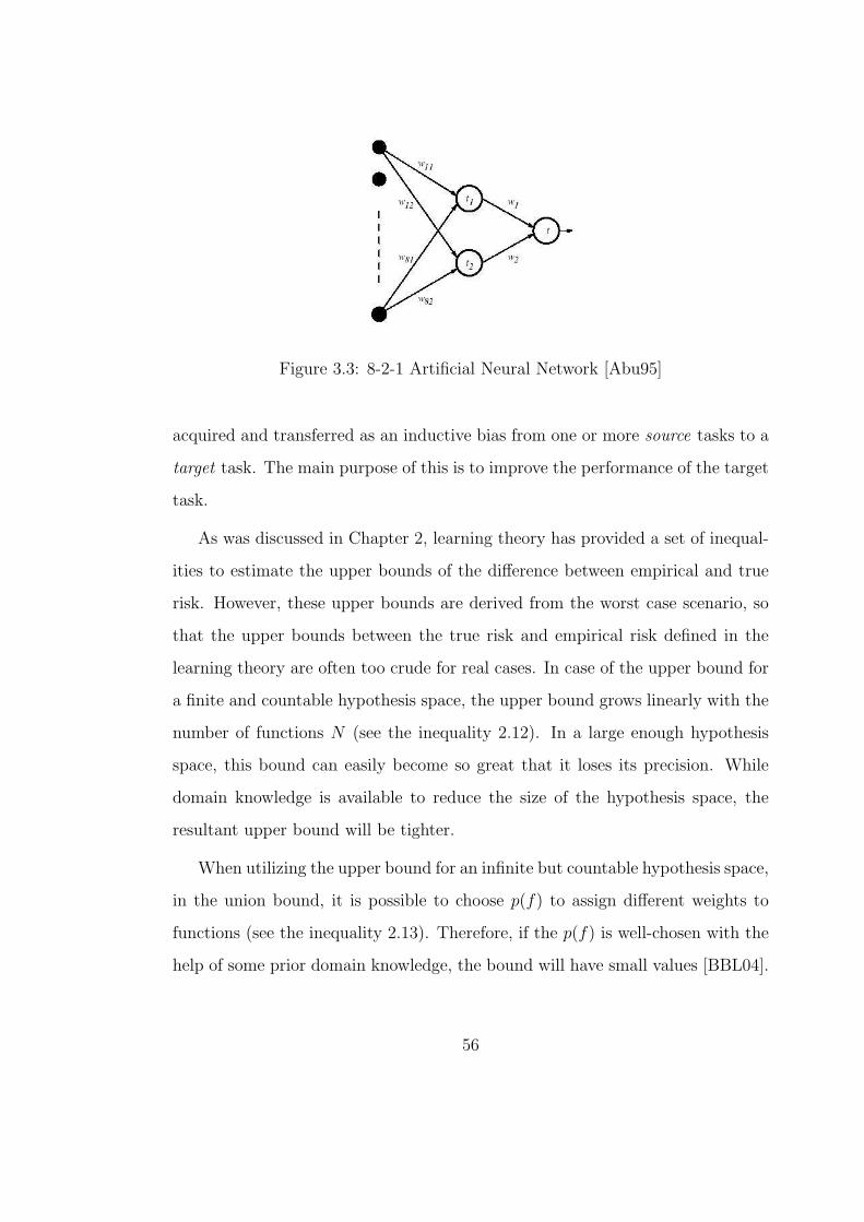
Figure 3.3: 8-2-1 Artificial Neural Network [Abu95]
acquired and transferred as an inductive bias from one or more source tasks to a
target task. The main purpose of this is to improve the performance of the target
task.
As was discussed in Chapter 2, learning theory has provided a set of inequal-
ities to estimate the upper bounds of the difference between empirical and true
risk. However, these upper bounds are derived from the worst case scenario, so
that the upper bounds between the true risk and empirical risk defined in the
learning theory are often too crude for real cases. In case of the upper bound for
a finite and countable hypothesis space, the upper bound grows linearly with the
number of functions N (see the inequality 2.12). In a large enough hypothesis
space, this bound can easily become so great that it loses its precision. While
domain knowledge is available to reduce the size of the hypothesis space, the
resultant upper bound will be tighter.
When utilizing the upper bound for an infinite but countable hypothesis space,
in the union bound, it is possible to choose p(f) to assign different weights to
functions (see the inequality 2.13). Therefore, if the p(f) is well-chosen with the
help of some prior domain knowledge, the bound will have small values [BBL04].
56
If the upper bound is utilized for an infinite and uncountable hypothesis space
as discussed previously, domain knowledge provides auxiliary information to es-
timate more precise upper bound than one only based on the given data (see the
inequality 2.17). Yaser Abu-Mostafa [Abu95] gave two general approaches to re-
duce generalization error by estimating new VC dimensions based on the data and
extra information: V C(H|K) and V C(H; K). The first one, V C(H|K), is defined
as the VC dimension of a hypothesis space in which any hypothesis h ∈ H satis-
fies the given domain knowledge K. Set H ′ represents the new hypothesis space
H ′ = h ∈ H ∧ h ° K and, for instance, the domain knowledge K can be an
invariance hint1. Since H ′ ⊆ H, it is clear that V C(H|K) = V C(H ′) ≤ V C(H).
For example, in Figure 3.3, there is an 8 − 2 − 1 artificial neural network with
8 input nodes, 2 nodes in the hidden layer and one output node. The number
of weights is 8 × 2 + 2 plus 3 thresholds. The VC dimension is approximately
V C(H) ≈ 21. Suppose the domain knowledge shows the parameters of an ANN
have special properties k1 : w11 = −w12, w21 = −w22, ..., w81 = −w82, t1 = t2,
w1 = w2, where wi is the weight and ti is the threshold. These special properties
reduce the number of weights and thresholds. Then, the new VC dimension of
the ANN, V C(H|k1) ≈ 8 + 1 + 1 = 10, is then less than the standard VC di-
mension 21 [Abu95]. The later one V C(H; K) arises when the virtual examples
are introduced as a proxy of the domain knowledge. By including extra artificial
examples, the number of total training examples increases, and V C(H; K) has a
upper bound 5V C(H) in case of the invariant hints [Fyf92]. With the increase
of the number n of the training examples, a parth(log 2en
h+1)−log(δ/2)
nof the up-
per bound decreases, and then the upper bound becomes more precise (see the
inequality 2.17).
1This hint asserts that c(x) = c(x′) for certain pairs x, x′. If this hint is violated, theassociated error is Rknowledge = (f(x) − f(x′))2. This hint will be discussed in detail in thefollowing section, ”Invariance”.
57

These discussed improvements to the upper bound provide only a framework
to incorporating auxiliary information thus reducing generalization errors. In
real-world cases, the effects vary depending on the different practical situations
and learning algorithms.
3.2.3 Convergence with Domain Knowledge
It is possible that domain knowledge enhances convergence to an optimal hypoth-
esis h(x) ∈ H which is equivalent to or the best approximation of the unknown
target hypothesis c(x).
The roles of domain knowledge in convergence addresses various characteris-
tics such as feasibility, efficiency, and accuracy. The feasibility indicates whether
the hypothesis space of the given learning algorithm can output a hypothesis
identical to the target model, and if that replica (or approximation) of the target
model is acceptable. In other words, the capacity of the hypothesis space deter-
mines the feasibility and also is addressed in the variance/bias tradeoff by the
generalization. If the given domain knowledge already indicates that the capacity
of the given hypothesis space does not reach certain requirements, the learning
algorithm already fails at the first place. No matter how much effort the learning
system puts into the convergence, a satisfying output will not be reached.
The efficiency of convergence is closely related to the complexity of the hy-
pothesis space, and directly determines the efficiency of the given learning algo-
rithm. With the help of certain domain knowledge, some learning algorithms can
initiate smaller and more precise hypothesis spaces. Others can reduce the size
of the hypothesis space, or select shorter (or more direct) search paths, whereby
convergence takes less computation time, and cost. There is, however, the pos-
sibility that when the domain knowledge introduces the auxiliary information,
58

it may increase the complexity of the learning process, thus causing the conver-
gence to be much slower, even becoming a NP-hard problem2. For example, if
a prediction process is represented as an optimization process and the domain
knowledge requires the result of the prediction process will be integers, the pre-
diction problem falls into an integer programming. The integer programming is
a typical NP-complete problem. Thus domain knowledge as an additional con-
straint increases the complexity of the prediction problem, but in terms of the
approximation to the unknown function c(x), this domain knowledge is of use.
In this case, the user has to make a trade-off between accuracy and cost.
Domain knowledge is a valuable tool in setting stop criterions of convergence
that also affects the accuracy of the convergence. This indicates how effective
the learned model (or selected function) is a replica of the target model. In
many practical learning problems, it is not economical to reach the best optimal
solution by using too much resource, such as computation time. There is a balance
between cost and accuracy, and domain knowledge can be valuable to set a set
of stop criterions to reach a cost-effective balance.
3.2.4 Summary
Along with the conceptual benefits of prior domain knowledge, there are two
key practical benefits namely: 1) eliminating noise from training example, and 2)
increasing the transparency of both the resultant models and the learning process.
The theoretic discussion relies on the assumption, that is there is no noise in the
training examples. In the majority of real-world cases, this assumption is not
2In complexity theory, NP (”Non-deterministic Polynomial time”) is the set of decisionproblems solvable in polynomial time on a non-deterministic Turing machine. The NP-completeproblems are the most difficult problems in NP in the sense that they are the ones most likelynot to be in polynomial time [AHU74].
59

valid, and many learning systems suffer from noisy training examples. In the
preprocessing of training examples, the domain knowledge plays a crucial role in
reducing the noise.
In many real-world cases, the opaque models, which the majority of complex
learning systems result in, are unacceptable. This is because it is very difficult for
naive users to accept an answer without a valid reason. This issue is often ignored
by academic researchers in the machine learning community, causing an obstacle
when complex learning system is implemented in industry. In industries, some
users prefer comprehensible simple models at the sacrifice of accuracy. This issue
is addressed in the following sections using semi-parametric modeling. It produces
a semi-transparent model, which reaches a balance between transparency and
accuracy. In the process of semi-parametric modelling, domain knowledge plays
a crucial role.
Along with the benefits, it is essential to discuss the risk of incorporating
domain knowledge. In the previous section on convergence with domain knowl-
edge, one risk has already been addressed: additional domain knowledge causes
intractable computation complexity. This issue assumes that domain knowl-
edge is perfect, in that it does not contain any noise and completely covers
the whole task. However, as for the imperfect training examples, imperfect do-
main knowledge is common in real-world practice. In order to minimize negative
impacts from imperfect domain knowledge, a trade-off is necessary. As previ-
ously discussed, one approach is the regularizer and employs a new risk function
wSRemp(f) + wKRknowledge(f), where the coefficients wS and wK assign the dif-
ferent weights to the empirical risk function Remp(f) and domain knowledge risk
function Rknowledge(f) (see Definition 2 in the section ”Consistency with Domain
Knowledge”).
60

Concerns about the consistency, generalization and convergence provide a
framework for the following methods of incorporating various prior domain knowl-
edge into inductive machine learning algorithms. In the following parts of this
thesis, all of the reviewed or proposed methods consider both this framework and
other relevant practical issues.
There are always a number of desirable properties sought after when forming
a learning algorithm. They include:
• Given no prior domain knowledge, a machine learning algorithm should
learn at least as effectively as purely inductive methods.
• Given a perfect domain knowledge, a machine learning algorithm should
learn at least as effectively as purely analytical methods
• Given an imperfect domain knowledge and imperfect training data, a ma-
chine learning algorithm should combine the two to outperform either purely
inductive or purely analytical methods.
• A machine learning algorithm should be tolerant to some unknown level of
error in the training data.
• A machine learning algorithm should be tolerant to some unknown level of
error in the domain knowledge [Mit97b].
Based on the essentiality of the domain knowledge in machine learning al-
gorithms, some machine learning algorithms require the domain knowledge as a
condition of learning. Others treat the domain knowledge as a option. Therefore,
domain knowledge is classified as ”required” and ”optional” domain knowledge
with respect to learning systems.
61
Based on the enforcement of the domain knowledge, some domain knowledge
is called ”hard domain knowledge” or ”strict enforcement”. Learning machines
must find ”best” feasible hypothesis being consistent with hard domain knowl-
edge. Other domain knowledge which learning machines find ”best” feasible
hypothesis maximally respecting is called ”soft domain knowledge” or ”partially
enforcement” [DR05].
The next section reviews and modifies Tom Mitchell’s categories of incor-
porating domain knowledge into machine learning, and includes recent research
results.
3.3 Using Prior Domain Knowledge to Preprocess Train-
ing Samples
The first step of the learning process of an inductive machine learning system
is to preprocess the training data. This step consists of selecting, cleaning and
transforming the original data.
The majority of learning algorithms assume that the collected training ex-
amples do not contain noises and the features have no redundance. In practice,
this assumption is not always established. In many cases, the noise introduced
by the examples or redundant features is the major cause of poor performance
in a learning system. Prior domain knowledge provides important information
to eliminate noise within the features and examples. Without sufficient domain
knowledge, one does not always know which indicators are relevant to the move-
ment of a particular response. Often one has to prepare different sets of indicators
and mine them [TYL04].
Before feeding data into any learning system, one often needs to experiment
62

Figure 3.4: Use virtual samples to bias the model produced by Support Vector
Machine [BS97] [SSS99]. The additional virtual samples force the resulting hy-
per-plane more horizontal than one produced by the original training samples at
the third figure.
with different ways to transform original data into new features, for example a
ratio of two features. One needs to remove the redundant features in order to
reduce the complexity. The most obvious observations to remove is the noise
thereby reducing noise and complexity. Some training examples have their in-
ternal structures, such as a tree or a network, and these structures need to be
transformed by domain knowledge in order to be incorporated into the learning
system. This research will use prior domain knowledge to guide the process of
feature selections, in the form of must-link (two features must be in the same
cluster) or cannot-link (two features must not be in the same cluster) .
Being different from the regular data preprocess, this section summarizes
some researches of incorporating prior domain knowledge into inductive machine
63

learning through data preparation. Among them, using virtual data samples
to influence the operation of search has gained much attention in recent years.
Partha Niyogi et al proposed an idea of virtual examples as a possible strategy
for incorporating prior information in the neural network in order to counter the
problem of insufficient training examples [NGP98]. This showed that the idea of
virtual examples was mathematically equivalent to incorporating prior domain
knowledge as a regularizer in the function learning in certain restricted domains.
Similar to Niyogi’s work, Bernhard Scholkopf et al pointed out that invari-
ance could be included in pattern recognition in a principled way via the vir-
tual support vector mechanism and restriction of the feature space (see Figure
3.4) [BS97] [SSS99]. Dennis Decoste et al inducted the invariant support vector
machine (SVM), which used prior knowledge as an invariance to bias SVM by
creating a series of virtual samples [DS02]. Their method is composed of the
following procedures:
1. train a Support Vector Machine to extract the support vector set;
2. generate artificial examples, termed virtual support vectors, by applying
the desired invariance transformations to the support vectors; and
3. train another support vector machine on the generated examples.
As the domain knowledge is encapsulated within a set of virtual examples, the
domain knowledge risk function is represented by an empirical risk of the vir-
tual examples Rknowledge(f(Xv)) = Remp(f(Xv)), where Xv is the set of virtual
examples.
The virtual training example method is an indirect way of incorporating prior
domain knowledge in a functional form. The strength of this method is that it
is a universal solution, so long as the given prior domain knowledge is able to
64

be converted into a set of artificial training data. In other words, this method is
feasible to any inductive learning system, which relies on the training data. But
this method also shares some of the drawbacks of functional knowledge transfer,
which requires more storage space and less computational efficiency in case of a
large volume of data.
3.4 Using Prior Domain Knowledge to Initiate the Hy-
pothesis Space or the Hypothesis
There are two types of approaches for using domain knowledge to initiate hypoth-
esis space or the hypothesis. The first approach is to initiate a hypothesis space
by satisfying both training examples and domain knowledge simultaneously. In-
ductive learning methods search out a hypothesis through this more appropriate
hypothesis space that is initiated partially or completely by the domain knowl-
edge. The hypotheses space is guaranteed to be consistent with the domain
knowledge. The second approach is to initialize the hypothesis either partially
or completely to fit the existing domain theory. Inductive learning methods will
be used to refine or complete the hypothesis by fitting the training data. In a
hypothesis space, this approach provides a better starting point for convergence.
A better starting point for convergence results in a closer replica to the unknown
target model; therefore, the path of convergence is shorter and the convergence
is more efficient.
In kernel-based learning algorithms which are data-based learning, the selec-
tions of their kernel function relies heavily on the domain theory. Without any
prior domain knowledge, it is common to choose the radial basis functions (RBF)
or polynomial functions as kernel functions. However, in many cases, it is better
65
to choose or create a special kernel function for particular requirements in certain
domains. Bernhard Scholkopf et al explored kernel designing, series of methods
for incorporating prior knowledge in constructing appropriate kernel functions
[SSS99]. Therefore, the kernels selected or constructed by the domain knowledge
initiate a proper hypothesis space in which learning algorithms converge to a
better approximation of the unknown target model.
Regular Bayesian Networks (BN) utilize existing domain knowledge to initiate
the structure of the network. The learning algorithms then parameterize the
network. In the structural learning of the Bayesian Network, Helge Langseth
and Thomas D. Nielsen used Object Oriented techniques to construct small and
”easy-to-read” pieces as building blocks for creating a more complex BN [LN03].
Beyond the simple sub-sections of BN, the OOBNs (Object Oriented Bayesian
Networks) introduce a class hierarchy in which the sub-superclass relationship
contains the domain knowledge about the structure of resultant BN. For example,
consider a farm with two dairy cows and two meat cows. Assume that the task
is to model the environment’s effect on the dairy and meat production of these
cows. The OOBNs construct a generic cow class (super class) that describes
the general properties common to all cows, and dairy cow and meat cow that
become two subclasses of that superclass. The subclasses inherit properties of
their superclass, and the OOBN framework facilitates the structural learning of a
Bayesian Network from training samples, simplifying the structure of the learned
network.
In the Knowledge-Based Artificial Neural Network (KBANN), a modified ar-
tificial neural network, an initial network is first constructed so that the classi-
fication assigned to every possible instance by the network is identical to that
assigned by the domain theory [TS89]. The Backpropagation algorithm is then
66

Figure 3.5: Different Invariance transformation [DS02]
employed to adjust the weights of this initial network as needed to fit the train-
ing examples. An assumption behind the KBANN is that the domain theory is
correct or approximately correct. Given a better starting approximation than
pure artificial neural network, the KBANN should learn better generalization
accuracy for the final hypothesis. However, the KBANN can be misled given
incorrect or insufficient prior knowledge [Mit97b]. In order to solve this problem,
the Explanation-Based Neural Network (EBNN) algorithm did not completely
rely on the users to provide prior knowledge, but calculated the prior parameters
by explaining each training example in terms of a given domain theory [Mit93]
[Thr96]. Similarly, Tony Jan et al used prior domain knowledge to build the
structure of a hypothesis and the neural learning refined the model [JYD04].
Patrice Simard et al and Partha Niyogi et al addressed the invariance in
the distance-based classification algorithms, for example K nearest neighbors
[SCD93][NGP98]. Suppose we know a transformation s (such as rotation) such
that if P is a valid example then s(P ) is also a valid example. The transformation
s depends on one parameter α, and the set of all transformed patterns SP =
x|∃α ⇒ x = s(α, P ) is an one-dimensional curve in the vector space of the
67

inputs. When the set of transformations is parameterized by n parameters αi,
SP is a manifold of at most n of P . The part of SP that is close to P can be
approximated by a plane tangent to the manifold SP at the point P . The regular
Euclidean distance between two patterns x and z is replaced by a new definition of
distance, the distance between two manifolds s(x) and s(z), called transformation
distance [SCD93]. The known invariance transformation could depend upon the
prior knowledge of a particular problem. For instance, in character recognition, a
small rotation and various thickness of a letter are typical invariances (see Figure
3.5), and we need a classifier that is invariant to those changes. By using the
transformation distance instead of the regular Euclidean distance, the hypothesis
space is initiated to be invariant to those changes.
The search objectives themselves are optimized by domain knowledge. For
example, the semantic query optimization introduced by Suk-Chung Yon et al
can be regarded as the process of transforming a query into an equivalent form
[YHP99]. This form can be evaluated efficiently by narrowing the search space
and refining the query. Suppose we consider the following domain knowledge:
all ships whose deadweight is greater than 700 tons travel at a speed greater
than 60 mph” and ”the ships whose deadweight is greater than 700 tons are
supertankers”. According to the domain knowledge, only ships whose type is
supertankers in the index of the shiptype need to be considered instead of the
speed and the deadweight.
68

3.5 Using Prior Domain Knowledge to Alter the Search
Objective
In this approach, the domain knowledge acts as an inductive bias in the process
of searching out an optimal hypothesis consistent with both the training data
and domain knowledge. Most learning algorithms convert their machine learning
problems into optimization problems by constructing objective functions with
sets of constraints. The problem of minimizing the empirical risk function is
an example of the objective function, min[Remp(f)] = min[∑m
i=1(yi − f(xi))2].
As the empirical risk function decreases, the learning algorithm converges to
a hypothesis which is the best approximation to the underlying desired model
within the given hypothesis space H. Here, the prior domain knowledge either
acts as an additional regularizer within the objective function or a set of additional
constraints. The majority of existing research on incorporating domain knowledge
into inductive machine learning occurs in this area, containing a diverse range of
results.
There are two major types of methods using prior domain knowledge to alter
the search objectives:
• The goal criterion is modified to require the output hypothesis to fit the do-
main knowledge as well as the training data; for example, learning with con-
straints [DR05][Abu95][SS02b], learning with weighted examples [WS04],
and cost-sensitive learning [Gio02].
• Domain knowledge is employed to verify the search result to guide the
search process in the right direction; for example, knowledge-guided learn-
ing proposed by Stuart Russell. Russell’s method generates all possible
hypotheses expressible in terms of primitive language and tests them for
69
consistency with its prior knowledge [Rus91].
3.5.1 Learning with Constraints
In practical problems, the hypothesis space can be vast. Therefore, it is necessary
to search the space preferentially and prune subspaces based on certain domain
knowledge. This is referred to as learning with constraints or constrained learning,
as addressed by Ian Davidson [DR05]. In learning with constraints, domain
knowledge is expressed as a set of additional constraints within the objective
function or constraint.
In handwritten characters recognition, certain derivatives of the target func-
tion can be specified in prior since some patterns of letters are available. This
approach has been explored by Simard et al. in TangentProp [SVC92]. In this
approach, an additional term is added into the error function of normal neural
learning to augument the search objectives. Thus, the Tangent Prop extends the
backpropagation algorithm, allowing it to learn directional derivatives. The usual
weight-update rule of the backpropagation algorithm is modified: ∆w = −η ∂E∂w
is replaced with ∆w = −η ∂∂w
(E + µEr), and the Er measures the discrepancy
between the actual and desired directional derivatives.
In the previous introduction to the kernel methods (see Section 2.3), the pa-
rameters w, d in the primal or α, d in the dual formula are solved as an
optimization problem, such as linear or quadratic programming. The basic idea
of the Knowledge-based Support Vector Machine (KSVM) as proposed by Glenn
M. Fung and Olvi L. Mangasarian is to include domain knowledge as extra con-
straints in the given linear or quadratic programming [FMS01] [MSW04]. In
order to narrow the hypothesis space, KSVM utilizes a set of linear equalities or
inequalities to represent prior domain knowledge in the properties of the target
70

functions.
3.5.1.1 Hints
Abu-Mostafa defined Hints as auxiliary information about the target function
that can be used to guide the learning process [Abu95], when the regular learning
process tries to recreate a target function using a set of input-output examples.
He listed some common types of hints:
• Invariance hint
This hint asserts that c(x) = c(x′) for certain pairs x, x′. If this hint is
violated, the associated error is Rknowledge = (f(x)− f(x′))2. This hint will
be discussed in detail in the following section, ”Invariance”.
• Monotonicity hint
This hint asserts for certain pairs x, x′ that f(x) ≤ f(x′). For instance, ”f
is monotonically nondecreasing in x” is formalized by all pairs x, x′ such
that f(x) ≤ f(x′). If this hint is violated, the associated error is
Rknowledge =
(f(x)− f(x′))2, if f(x) > f(x′)
0, if f(x) ≤ f(x′)(3.4)
Joseph Sill el at incorporated the monotonicity hints into the backprop-
agation algorithm for credit card fraud detection [SA97]. The resultant
improvement from the introduction of monotonicity hints is statistically
significant, nearly 2%.
• Examples hint
Given (x1, c(x1)), . . . , (xN , c(xN)), the examples hint asserts that these are
the correct values of c at the particular points within x1, . . . , xN . Say that
71

the correct subset consists of n examples: (x1, c(x1)), . . . , (xn, c(xn)), and
then if this hint is violated, the associated error is Rknowledge = (f(xn) −c(xn))2.
It is worth highlighting the difference between examples hint and previous
virtual example method (see Section 3.3 “Using Prior Domain Knowledge
to Preprocess Training Samples”). The former randomly picks up a subset
of the examples, and the learning algorithm will put more heavy penalty
to the violation of this subset. In the contrary, the virtual example method
adds extra virtual examples apart from the original training examples.
• Approximation Hint
The hint asserts for certain points x ∈ X that c(x) ∈ [ax, bx]. In other
words, the value of c at x is only known approximately. If this hint is
violated, the associated error is:
Rknowledge =
(f(x)− ax)2, if f(x) < ax
(f(x)− bx)2, if f(x) > bx
0, if f(x) ∈ [ax, bb]
(3.5)
• Consistency Hint
The consistency hint differs from previous hints, in that it is more subtle.
Including a consistency hint forces the learning algorithms to be consistent
with their theoretic assumptions. The parametric models always make the
assumption that the model is based on. For example, the discrete time ver-
sion of stochastic Vasicek model ∆xn[l] = kn(θn−xn[l]∆t[l]+σnwn[l]√
∆t[l])
has assumptions that wn[l] follows a gaussian distribution. However, within
the learning process, there is no discrepancy metric between the learned dis-
tribution and theoretic assumptions. Abu-Mostafa employed the Kullback-
72

Leibler distance K(p‖q) to quantify the agreement/disagreement between
the two distribution:
K(p‖q) =
∫p(u)log
p(u)
q(u)du (3.6)
here p(u) is the pdf of the learned w[l], q(u) is the pdf of the theoretical
w[l] [Abu01]. Since the form of p(u) is unknown, the maximum-entropy
principle is used to estimate it. Therefore the risk function of this consis-
tency hint is expressed as Rknowledge = K(p‖q), and if and only if p = q the
Rknowledge = K(p‖q) = 0. It is simple to inject this risk function into the
original objective function.
• Catalytic Hint
The catalytic hint is also quite different from the previous hints. The major
difference comes from the way in which the catalytic hint is incorporated.
As introduced by Steven Suddarth and Alistair Holden [SH91], the catalytic
hint was first realized in the feed-forward neural network and later imple-
mented by Yaser Abu-Mostafa [Abu95] and Yaochu Jin [JS99] respectively.
They introduced additional output nodes, catalytic neurons (see Figure
3.6), which are only included by artificial neural networks during the train-
ing process. The additional catalytic nodes force the neural network to
learn extra functions simultaneously with the target function. In practice,
the extra functions are closely related to the target function. By using the
catalytic hints, users emphasize in some parts of the target function.
When hints are available in a learning situation, the objective function, as
optimized by the learning algorithms, is no longer confined only to the empirical
risk Remp [Abu95]. The associated domain knowledge risk function Rknowledge with
hints is then included as extra components in the objective function to contain
73

Figure 3.6: Catalytic Hints [JS99]
the information with hints. Further, the ”hints” approach could be treated as a
special case in the regularization theory. Here an ill-posed problem is transformed
into a well-posed one by using prior domain knowledge. The most common form
of prior knowledge is smoothness, but others include monotonicity, convexity and
positivity [NGP98]. In terms of the optimization theory, these approaches either
modify the objective function, or introduce extra constraints into an optimization
problem.
3.5.1.2 Invariance
In recent years, the machine learning community put a large amount of emphasis
on invariance. The invariance means the information of certain transformations of
the input which are known to leave the function values unchanged. For example,
in the figure 3.5, artificial data is generated by rotating a digital image of the digit
“5”. An invariant machine learning algorithm has the capability of recognizing
this artificial data as the digital image of the digit “5” instead of other digits. By
74
revisiting the previous definition of ”Invariance Hints”, a certain pair x, x′ stands
for the digital image of the digit ”5” and the rotated image of 3 degrees. Because
the two images are the same c(x) = c(x′), the correct learned hypothesis then
produces: f(x) = f(x′) and the associated error is em = (f(x)− f(x′))2 = 0.
The virtual example method is one of approaches to incorporating invariance
into regular inductive machine learning. However it has two major drawbacks:
1) the users must choose the magnitude of distortion and how many virtual
examples should be generated; and 2) more importantly, the virtual example
is highly correlated with the original data. This makes some of the learning
algorithms, such as ANN, very inefficient [SVC92].
Bernhard Scholkopf et al summarizes three types of methods for incorporating
invariance into kernel methods [SS02b]. First there are the virtual support vector
method, as discussed in the previous section (see Section 3.3); then Jittered SV
method, as will be discussed in the following section (see Section 3.6). Finally
the invariance hyperplane method can be seen as a extension of previous hints
method. The basic idea is to introduce an additional regularizer into the regular
objective function. The linear decision function (see equation 2.22) is rewritten
as f = sgn g, where g(xj) :=∑m
i=1 αiyi〈Bxj, Bxi〉 + b with a matrix B to be
determined.
The definition of invariance indicates that local invariance of g or each pattern
xj under transformations of a differentiable local 1-parameter Lie group3 of local
transformations Lt, will lead to g(xj) − g(Ltxj) = 0. The results of the deci-
sion function between the original pattern xj and the transformed pattern Ltxj
have no difference. Thereby, the local invariance of g or each pattern xj under
3The theory of Lie groups ensures that compositions of local (small) transformations si
correspond to linear combinations of the corresponding tangent vectors (local transformationssi have a structure of Lie algebra); for example, the transformations of a differentiable local1-parameter Lie group of local transformations Lt [SS02b].
75

transformations of a differentiable local 1-parameter Lie group of local transfor-
mations Lt is ∂∂t|t=0g(Ltxj) = 0. It can be approximately enforced by minimizing
a regularizer: 1m
∑mj=1(
∂∂t|t=0 g(Ltxj))
2 [SS02b][SSS99].
3.5.2 Learning with Weighted Examples:
As it is relatively straightforward to add extra constraints in an optimization
problem, learning with constraints has already produced some relatively mature
results. Learning with weighted examples is another often-used method of ma-
nipulating the objective function to contain extra information.
Xiaoyun Wu and Rohini Srihari developed a new derivative of the SVM, the
Weighted Margin Support Vector Machine (WMSVM) [WS04]. They used prior
domain knowledge to generate ”Pseudo Training Dataset” as a part of training
sample input into the WMSVM. The objective function of primal problem of the
WMSVM is given:
〈w · w〉+ C
m∑i=1
ξi + ηC
n∑i=m+1
g(vi)ξi (3.7)
where the parameter C controls the balance between the model complexity and
training error, g(vi) is the slack normalizaion function for the soft margin algo-
rithm, and the extra parameter η is used to control the relative importance of the
evidence from these two different datasets, that are the true training examples
and Pseudo Training Dataset. One wants to have a relatively bigger η when the
quality of true training examples is poor. Wu and Srihari carried two experi-
ments of text categorization, and compared to the results from a standard SVM,
LibSVM [CL01], WMSVM with prior knowledge achieved higher accuracy with
much less training samples [WS04]. Their experimental outcomes supports the
hypothesis of this thesis.
76

Considering the importance of order in the time-series analysis, L. J. Cao et
al incorporated time orders as a parameter of regularized risk function of SVM
to put heavier weights to the recent training samples than those of the distant
training data points [CT03].
3.5.3 Cost-sensitive Learning
Cost-sensitive classification problems are characterized by different costs for dif-
ferent classification errors [Gio02]. Let c(i, j) be the cost of deciding for class i
when the true class is j. The empirical risk is rewritten as:
Remp =m∑
j=0
c(i, j) (3.8)
Cost-sensitive learning is very close to the learning with weighted examples,
but differs in that it is restricted within the classification problems as cost-
sensitive regression has intractable computation cost. Giorgio Fumera et al im-
plemented cost-sensitive learning into a binary SVM, and the empirical function
becomes: suppose the decision function is defined:
f(x, α) = +1, if w · x + b ≥ ε
f(x, α) = 0, if −ε < w · x + b < ε
f(x, α) = −1, if w · x + b ≥ −ε
(3.9)
and the empirical risk function will be:
Remp =
0, if f(x, α) = y
cR, if f(x, α) = 0
1, if f(x, α) 6= y and f(x, α) 6= 0
(3.10)
where ε delimits a ”reject” area along the hyperplane. The examples located
within the reject area will be handled with different procedures [Gio02].
77

3.6 Using Domain Knowledge to Augment Search
Using domain knowledge to augment search is similar to using prior domain
knowledge to alter the search objective. The difference is that the methods of
using domain knowledge to augment search produce new hypothesis candidates
in the process of searching (or convergence). In other words, the hypothesis
space H is adjusted by the domain knowledge with the on-going searching. But
the methods of using prior domain knowledge to alter the search objective work
within a fixed hypothesis space and the domain knowledge only eliminates parts
of the hypothesis space.
Pazzani et al [PBS91] developed the FOCL as an extension of the purely
inductive FOIL system. FOIL generates hypotheses purely from training data.
FOCL also use domain knowledge to generate additional specifications, but it
then selects one hypothesis among all of these candidate specifications based on
their performance over the data. Therefore, in the FOCL method, imperfect
domain knowledge only impacts the hypotheses if the evidence in the data sets
supports the knowledge.
In kernel methods, Dennis Decoste et al introduces the idea of ”kernel jitter-
ing” [DS02]. Prior domain knowledge is included by applying transformations to
patterns as a part of kernel definition. In SVM, this method replaces the regular
kernel function, K(xi, xj) ≡ Ki,j as a jittering kernel form KJ(xi, xj) ≡ KJi,j,
defined procedurally as follows:
1. Consider all jittered forms (see Figure 3.5) of example xi (including itself)
in turn, and select the one (xq) ”closest” to xj; specifically, select xq to
minimize the metric distance between xq and xj in the space induced by
the kernel. The distance is given by:√
Kqq − 2Kqj + Kjj.
78

2. let KJij = Kqj
According to their experiment which compares the performance between the
virtual SV (VSV) and the kernel jitter, the training set of the kernel jitter can be
smaller than the corresponding VSV methods, but its accuracy was lower than
the VSV methods.
A limited amount of research has been done in this category, as it is difficult to
simultaneously adjust both the process of convergence and the hypothesis space.
The majority of inductive learning algorithms do both separately.
3.7 Semi-parametric Models and Hierarchical Models
Traditional statistics methods which make assumptions regarding underlying dis-
tributions are named parametric methods . The term ”parametric” indicates that
the structure of the resultant model is known, and the learning methods only esti-
mate the parameters of the resultant models. In contrast, most machine learning
methods exist as non-parametric methods , which simply use very complex struc-
tures and do not make any assumption of the underlying distribution, or the
structures of the resultant models. In theory, they provide universal approaches
independent from the domain, but in reality they introduce higher computation
and complexity without the transparent structures of resultant models. For ex-
ample, kernel methods use a set of basis functions, to approximate the underlying
distribution. The cardinal number of the set of basis functions may reach infinity.
If the structure of the resultant model is known beforehand, the parametric
method is preferred. This is because the structure of resultant model is more com-
prehensible and its computation is more efficient than non-parametric methods.
In real world examples, some domains have been explored and some parametric
79

models exist but often they are incomplete. One solution is to apply parametric
knowledge to the problem as much as possible in order to represent the known
knowledge. The nonparametric techniques would then address the remainder of
the question. This kind of hybrid model is called as semi-parametric model (or
hierarchical models) and depends on the structure of its resultant models.
A semi-parametric model consists of the parametric components and nonpara-
metric components. A semi-parametric model contains the following structure:
f(x) = g(xm) +∑n
i=1 βixi, where xm, xn ⊆ x, g(xm) is the nonparametric
component, and∑n
i=1 βixi is a linear parametric component with xi ∈ xn. Semi-
parametric models are easy to understand (due to the parametric part), and
perform well (often thanks to the nonparametric term) [SS02a]. When the non-
parametric component is a support vector regression (SVR), a semi-parametric
SV regression introduces additional components within the constraints when the
setting is translated into optimization problems. In terms of the capacity of
the function class, kernel mapping in nonparametric components produces much
higher dimensions than that of parametric components. Thus even if the paramet-
ric components are not regularized at all, the overall capacity still works [SS02a].
In a similar research in the SVM, Davide Mattera and Francesco Palmieri intro-
duced the semi-parametric SVM as a general structure of nonlinear functions,
f(x) = wT φ(x) + wT1 ψ(x), in which wT
1 ψ(x) embedded prior known parametric
function [MPH01]. These two research methods achieved the same result in two
different ways.
Hierarchical models address the fundamental assumptions in the majority of
machine learning algorithms, as with identical underlying distribution. In many
cases, it is certain that data is not produced by identical distribution, but by
related data sets. Rather than using a single model to cover all data sets, it
80

is more sensible to build a set of different local models, and then use a global
model to unify them. The hierarchical models constructed by nonparametric and
parametric components belong to semi-parametric models.
In some literature, the hierarchical Bayesian modelling allows the informa-
tion between different models to be transferred via common hyperparameters.
For example, they assume that M data sets DjMj=1 are available for related but
not identical settings and they have trained M different models with parameters
θjMj=1 on those data sets [TY04]. If a new model concerns a related prob-
lem, then it makes sense to select new hyperparameters hhb such that P (θ|hhb)
approximates the empirical distribution given by the maximum likelihood pa-
rameter estimate instead of using the original informed prior P (θ|hprior). In this
way the new model can inherit knowledge acquired not only from its own data
set, but also from the other models: θM+1: P (θM+1|DjMj=1) ≈ P (θM+1|hhb). In
order to realize this inheritance, the local models must share the same or similar
parametric structure. Otherwise the inheritant is difficult.
The hierarchical models allow the ”knowledge transfer” via common hyper-
parameters within their framework. This is a very attractive characteristic in
that each local model represents one subset of data produced by an identical
distribution. The global model then works like a collaborative filter to transfer
knowledge amongst the local models. Clearly, it is closely related to the previous
multi-task learning.
As with audit fee estimation, current researches construct a single model to
estimate the audit fee of all of the listed companies in the Australian Stock Ex-
change (ASX). However, it is well-known that different industries have different
auditing standards, and further that large companies have different auditing stan-
dards from small or medium size companies. Therefore it is wise to construct a
81

local model for a subset of observation, an industry category, and then construct
a global model covering all local models. When a new subset of observations,
such as industry category, is collected, the global model initiates a local model
via transferring knowledge from other local models.
3.8 Incorporating Financial Domain Knowledge into In-
ductive Machine Learning in Capital Markets
In this thesis, most experiments are based on applications on capital market
domain. Capital markets are the part of financial markets that house a set of
institutional arrangements to facilitate the transfer of funds among the investors
[McI00]. Furthermore, the capital markets are the financial markets for their
instruments with an initial life of one year or more [CJ05]. In the capital mar-
kets, the financial instruments include equities (shares, or stocks), fixed-income
securities, derivatives and money. Because of the availability of the data, in this
thesis only the equity markets are concerned.
A company that has its shares quoted on a stock exchange is known as a
publicly listed corporation. A number of important roles are played by stock
markets. In order for a stock exchange to compete within the global market, it
must have systems in place that facilitate an efficient market. The Australian
Stock Exchange (ASX) operates on electronic trading systems, known as SEATS.
For a stock market to be efficient, it must be fully informed. The listing rules
of an exchange will require a corporation to advise the exchange, and therefore
the markets, of its half-yearly and annual financial statement. They are also
required to report any material change that might impact the share price of the
corporation immediately as it becomes evident. The ASX and Australian Se-
82

curity and Investment Commission (ASIC) supervise the overall integrity of the
markets [CJ05]. In this thesis, two case-studies include first the impact measure-
ment of unexpected information releases, such as price sensitive announcements,
on the corresponding stock price movements, and second the detection of the il-
legal behaviors with earnings management in the half-yearly and annual financial
statements from listed companies in the ASX.
Some machine learning methods have already been used for decision support
tools in Capital Markets research and practices [GT00]:
• Traditional statistics : linear, quadratic and logistic discrimination, regres-
sion analysis, MANOVA, etc [JW01].
• Modern statistics : K-Nearest-Neighbours, projection pursuit, ACS, SMART,
MARS, etc [WK91] [McL92] [MST94].
• Decision tree and rule-based induction methods : CART, C5.0, decision
trees, expert systems [MST94] [Mit97b].
• Neural networks, Support Vector Machine and related methods : feedfor-
ward ANN, self-organized maps, radial base functions, etc. [Mit97a] [CT03]
[Zha00].
• Bayesian Inference and Networks [CL96] [FPS96] [BH02].
• Model combination methods : boosting and bagging [FS95] [Bre96a].
The first attempt of incorporating financial domain knowledge into inductive
machine learning appeared in Yaser Abu-Mostafa’s works over the artificial neu-
ral networks (ANN) [Abu95]. In this paper, he described a symmetry hint can
be applied to forecasting in the foreign exchange markets, as a type of domain
83

knowledge. A symmetry hint asserts that if a pattern in the price history implies
a certain move in the market, then this implication holds whether you are looking
at the market from the U.S. Dollar viewpoint or the German Deutchmark view-
point. In terms of normalized prices, the hint formally translates to invariance
under inversion of these prices [Abu95]. Boris Kovalerchuk et al showed that
financial time series can benefit significantly from relational data mining based
on symbolic methods, as symbolic methods, such as first-order logic, prevail in
the areas with nonnumeric symbolic knowledge [KV00][KVY02].
The application of the domain knowledge to capital markets is valid in in-
ductive machine learning due to specific characteristics of capital markets. Often
the accuracy of the classification in the financial domain reaches only 50%. How-
ever, the accuracy is often close to 100% in optical character recognition. When
compared with the performance in the optical character recognition, the result
in capital markets is unacceptable. The major reasons include: limited, noisy
and non-stationary observations, as pure data-driven learning methods need suf-
ficient and clean data for training and verification [Abu95]. Additionally, any
capital market can be viewed as a system that absorbs types of information
(fundamentals, news events, rumors, traders’ behaviors etc.) and produces an
output (say up/down price movement for simplicity). The unobserved informa-
tion cannot be modeled and introduces noise. At the same time, there is a large
amount of research accumulated by financial researchers and participators. For
example, within past years, time-series models, such as ARMA-GARCH, have
demonstrated their power of exploring the underlying interrelationship between
different financial indicators [CLM97]. Abu-Mostafa’s experiments over foreign
exchange markets demonstrate that even a simple domain knowledge is able to
enhance the performance of regular learning algorithms dramatically.
84

3.9 Summary
This chapter presents a framework for incorporating prior domain knowledge into
inductive machine learning algorithms in three key issues: consistency, general-
ization and convergence. Furthermore, the framework is employed to summarize
four major categories of combination methods. According to this summary, al-
most every machine learning algorithm has its way of incorporating prior domain
knowledge into itself, and there is not a universal approach which covers various
machine learning techniques. For example, the idea of Object Oriented Bayesian
Network (OOBN) is unsuitable to kernel methods, because they do not contain
such complex network structures as BNs do. Similar types of domain knowledge
may be incorporated in different ways into the same learning algorithm. For ex-
ample, there are three ways of incorporating the invariance into kernel methods:
virtual examples, the invariance hyperplane, and the Jittered SV methods. The
selection of the method depends on the requirements of a particular task.
In terms of two major learning algorithms, the difference between the kernel
methods and the Artificial Neural Network posits that the methods incorporating
the domain knowledge into the ANN might be unsuitable to kernel methods. For
example, the structure of hypothesis of the ANN and kernel methods are different,
as the ANN has a network structure with or without hidden layers but the kernel
methods implement the mapping from the input space to the feature space. Thus,
the idea of the KBANN, basically initiating a network structure with the domain
knowledge, is unable to be implemented to the kernel methods.
The modularity of kernel methods shows itself more flexible learning proce-
dures than the ANN (see Figure 2.3) [SC04]. The whole learning procedure can
be decomposed into a sequence of modules, such as kernels, hypothesis spaces
and optimizations. All modules are relatively independent from each other. The
85
same algorithm can work with any kernel and hence for any data domain. The
kernel component is data specific, but can be combined with different algorithms
to solve the full range of tasks that we will consider [SC04]. This modularity
coincides very well with the previous four categories of incorporating domain
knowledge into inductive machine learning. It is straightforward to apply one
of the four categories in the corresponding module of the kernel methods. All
this leads to a very natural and elegant approach to learning system design for
incorporating prior domain knowledge.
The majority of machine learning methods have to be tailored in order to
contain the given domain-specific knowledge, with the modification depending
on the machine learning algorithm itself and the characterization of the given
domain knowledge. The framework introduced in this chapter forms the basis on
which any modification should be made. The same as other inductive machine
learning algorithms, kernel methods have to be tailored in many domains. Even
though the current research has produced a significant amount of methods, they
are still limited within certain domains, such as pattern recognition. As was
discussed in the previous section (see Section 3.8), the current implementation
of machine learning in the Capital Markets is not so successful as some of other
domains. One of potential ways of improvements is to incorporate prior domain
knowledge into itself. Regarding the characteristics of domain knowledge in the
Capital Markets, particular methods are necessary and need to be developed to
maximize the performance of the kernel methods. In the following chapters, new
methods are presented and tested on the data set from Capital Markets. The
new methods show how to incorporate domain knowledge into inductive machine
learning with efficiency and effectiveness.
86

CHAPTER 4
Methodology
This chapter proposes three new methods of incorporating various prior domain
knowledge into the kernel methods. In the first method, prior domain knowledge
is expressed in the format of local parametric models and partition functions
in the semi-parametric hierarchical model. The domain knowledge is utilized
to initiate the hypothesis space, which is a class of semi-parametric hierarchical
models. In the second method, prior domain knowledge is encoded in the format
of the interrelationship amongst features (or variables). Instead of probabilities,
the interrelationship is represented as a set of must-link and must-precede clauses
in the learning process. For example, it is usual for a feature x1 to be related
to another feature x2. According to the previous categories of incorporating
domain knowledge into inductive machine learning, in this method, prior domain
knowledge is employed to guide the learning process and verify the hypothesis
produced by the learning algorithm. This is similar to the knowledge-guided
learning as addressed by Stuart Russell [Rus91]. In the third method, prior
domain knowledge is represented in the format of logic clauses and is used to
prepare the training examples by labeling the unlabeled training examples which
are then fed into a supervised learning algorithm. In this case, domain knowledge
is encapsulated in training examples as a complement with the resultant model
being consistent with both observations and domain knowledge.
87

4.1 Semi-parametric Hierarchical Modelling
As was discussed in the previous chapter, hierarchical modelling provides a frame-
work to contain the domain knowledge represented within the local models. At
the same time, the global model works as a collaborative filter that transfers the
knowledge amongst the local models in formats of the hyperparameters. With
sufficient domain knowledge, many of the local models have rather transparent
structures. Even if the domain knowledge does not cover the domain completely,
it is still possible to find a sub-region covered adequately by domain knowledge.
Given sufficient domain knowledge, parametric models can be sensible choices,
however, many domains often lack existing domain knowledge to describe the
underlying patterns for parametric modeling. Even sometimes, the distributions
are not identical. Under this circumstance, the nonparametric model is a bet-
ter choice as it does not make any unreasonable assumption of the unknown
underlying distribution.
The basic assumption of parametric statistical models is that they are de-
fined by using a fixed number of parameters regardless of the number of training
examples. Thus the parameters provide a finite summary of the data. In the
nonparametric models, the number of parameters in the model is allowed to grow
with the size of the data set. With more data, the model becomes more complex,
with no a-priori limit set on the complexity of the model [Gha04].
The concept of non-parametric hierarchical modelling has been discussed by
Volker Tresp et al [TY04]. They used the Dirichlet distribution as a nonpara-
metric global model. In this section, the kernel methods are used to construct
the global model. In many studies, this kind of “mixed” model is named the
semi-parametric model.
88

There are benefits to working with a semi-parametric hierarchical model . For
example, users control the complexity of the model by controlling the partition-
ing and the structures of local models. It is worth clarifying that local models
are not restricted by parametric models. If there are no sufficient domain knowl-
edge in a sub-region of data, then it is sensible to use non-parametric modelling
to avoid utilizing unreasonable assumptions. But parametric local models are
highly recommended where appropriate because of their simplicity and inherent
transparency.
Apart from the selection of local and global models, another important issue
to building a successful hierarchical model is by partitioning the original obser-
vations. Depending on the partitions, hierarchical modelling produces two types
of structures:
• Feature Partitioning
If the features are partitioned into several subsets and the ”local” mod-
els represent the parametric interrelationships amongst features within a
subset of features, the overall model is equivalent to the semi-parametric
model as defined by Smola [SFS98]. The semi-parametric model con-
tains the nonparametric components and parameter components: y =∑m
i=1 βixi +g(xm+1, . . . , xn), where∑m
i=1 βixi is the parametric component,
g(xm+1, . . . , xn) is the non-parametric component.
• Observation Partitioning
If the observations are partitioned into several subsets and the local mod-
els represent the different interrelationships amongst the features within
that subset of observations. The previous hierarchical Bayesian Network
is an example of this model. This type of model can be written as: y =
89

f(h1(x), . . . , hi(x)), where hi(x) is the set of the local parametric models.
The way of partitioning is represented by a partition function (or switch func-
tion) which assigns observations to local models. The partition function may em-
ploy different subsets of training data from those used by local models. Either the
model selection or the partition of the original observation requires the presence
of domain knowledge in the format of parametric local models or the information
of partitions. The local models are then unified by the global model.
4.1.1 Vector Quantization
Vector quantization (VQ) is a lossy compression method based on the principle
of vector component analysis. According to Shannon’s theory of data compres-
sion, in the lossy data compression, better known as rate-distortion theory, the
decompressed data does not have to be exactly the same as the original data.
Instead, some amounts of distortion D are tolerated, and in contrast the lossless
compression has no distortion, D = 0.
Linde, Buzo, and Gray proposed a VQ design algorithm based on a training
sequence. The use of a training sequence bypasses the need for multi-dimensional
integration required by previous VQ methods [LBG80]. A VQ that is designed
using this algorithm is referred to in relevant literature as an LBG-VQ (see Figure
4.1). Given a vector source with its statistical properties known, a distortion
measure, and the number of codevectors, the LBG-VQ finds a codebook (the set
of all red stars) and a partition (the set of blue lines) which result in the smallest
average distortion [GG92].
Consider a training sequence consisting of M vectors: T = x1, x2, ..., xM,and N codevectors C = c1, c2, ..., cN. The whole region is partitioned by the
90

Figure 4.1: A Simple Example of Two-dimensional LBG-VQ [GG92]
codevectors into a set of sub-regions, called Voronoi Regions P = S1, S2, ..., SN.Vectors within a region Sn are represented by their codevector Q(xm) = cn as
xm ∈ Sn, and the average distortion can be given by: Dave = 1Mk
∑Mm=1 ‖xm −
Q(xm)‖, which measures the information loss. Thus, the design problem can
be summarized as: argminC,P (D) that is to estimate C and P such that D is
minimized.
If C and P are a solution to the above minimization problem. First, it must
satisfy two criteria: the nearest neighbor condition, Sn = x : ‖x− cn‖2 ≤ ‖x− cn′‖2,
∀n′ ∈ 1, 2, ..., N. Second, the centroid condition, cn =P
xm∈SnxmP
xm∈Sn1
, ∀n ∈1, 2, .., N. According to the defined framework of the semi-parametric hier-
archical modelling, the LBG-VQ acts as a partition function, the local model
represents a subregion Sn by its codevector Q(xm) = cn, and the global model is
represented by a support vector machine.
The LBG-VQ design algorithm is iterative, which alternatively solves the
91

above two optimization criteria. The algorithm requires an initial codebook that
is obtained by a splitting method. The initial codevector is set as the average of
the entire training sequence, and then split into two with the iterative algorithm
running with these two vectors as the initial codebook. The final two codevectors
are split into four, four into eight, eight into sixteen, and the process is repeated
until the desired number of codevectors is obtained [GG92].
4.1.2 VQSVM and Semi-parametric Hierarchical Modelling
In the case of binary classification SVM, the original decision function of support
vector machine (Equation 2.22) is rewritten as:
f(x) = sgnw · φ(x) + b = sgnM∑
j=1
αjyjk(x,Qj(x)) + b (4.1)
where Qj(x) stands for the sub-models, and the various sub-models provide the
flexibility to contain the different local information. Here the local models are
restricted by parametric models, in order to improve the performance of model.
The original learning function (Equation 2.21) is rewritten as:
Θ(α) = minw,bL(w, b, α) = −1
2
M∑i,j=1
αiαjyiyj〈Qi(x) ·Qj(x)〉+M∑
i,j=1
αi (4.2)
where Qi(x) and Qj(x) represent two different local models.
As the original training data set is partitioned by vector quantization, each
local model is a Voronoi Region Sj, which is represented by its codevector, Qj(x).
For example, a sum-average of the original observation within a cluster can be
expressed as:
Qj(x) = cj =
∑xm∈Sj
xm
N,m = 1, 2, .., N (4.3)
where N becomes the number of observations in the cluster Sj. If a training obser-
vation xm belongs to the cluster Sj, it is replaced by the codevector Qj(xm) = cj
92

Figure 4.2: Hierarchical Modelling with SV Machines, which modifies the original
SVM (see figure 2.3)
in the following SVM model. Note the VQ functions are substituted into the
previous decision function:
f(x) = sgnw · φ(x) + b = sgnM∑
j=1
αjyjk(x, cj) + b (4.4)
The VQSVM contains a semi-parametric hierarchical structure combining a
set of local models represented by codevectors, and a global model represented
by an SVM. In this thesis, this type of mixture model is classified as a semi-
parametric model, as the SVM is a well-known nonparametric model and the VQ
is a parametric model with a rather transparent structure.
This semi-parametric hierarchical model is a way of incorporating prior do-
main knowledge into inductive machine learning. The domain knowledge indi-
cates there is a set of related, but not identical distributions. Each distribution
is represented in formats of a local parametric model, which the global model
then explores the unknown information. As an example of the semi-parametric
hierarchical model, the VQSVM incorporates the prior domain knowledge, that
93

is a set of related but not identical distributions, into an inductive machine learn-
ing algorithm that is an SVM. This is facilitated by the partition of observations
done by the VQ and local parametric models constructed by codevectors.
4.1.3 Remarks of the Proposal Model
The proposed semi-parametric hierarchical modelling has multiple advantages.
First, the hypothesis space of the VQSVM is initiated by both the training exam-
ples and the domain knowledge, as its kernel is constructed as k(Ql(xi), Ql(xj)).
Thus the resultant model is consistent with both observations and domain knowl-
edge. Second, the resultant model contains less SVs, reducing the VC dimension.
This results in the model having a better generalization. The kernel mapping is
expressed mathematically as: φ : x → (√
λjψj(x))j, j = 1, . . . , N , but φ is un-
known and computationally expensive, especially when it maps into a space with
infinite dimensions. In practice, the mapping φ is approximated by the empirical
kernel mapping, that is:
For a given set z1, . . . , zm, we call φm : RN → Rm, x 7→k(., x)|z1,...,zm = (k(z1, x), . . . , k(zm, x)) the empirical kernel mapping
w.r.t. z1, . . . , zm [SMB99].
The feature space (a Hilbert space) is spanned by the mapped training exam-
ples. In practice, z1, . . . , zm is constructed by a set of support vectors (SVs).
Thus reducing the number of SVs decreases the dimensions of the resultant fea-
ture space.
Third, in equation 2.22, the computation cost of∑n
i=i αiyik(x, xi) is deter-
mined by the n, that is the number of the SVs. The reduction of the number n
of SVs decreases the complexity of the resultant model. Thus, the whole model
94

is more efficient, simpler and more transparent.
However, this successful method has its limitations. For example, only the
training examples are partitioned by the VQ. In case of the binary classification,
the VQ is carried over into the positive and negative classes of training examples
respectively. After the VQ, the new training examples are fed into the SVM for
modelling. In the prediction, the new observation is fed into the SVM model
without going through the VQ. In this sense, the VQSVM is not typical example
of hierarchal modelling.
4.2 A Kernel Based Feature Selection via Analysis of Rel-
evance and Redundancy
Peter Cheeseman suggests that all effects that have not been modelled add to
the noise term [CS96]. Irrelevant features introduce noise into the learning pro-
cess, also degrading the performance. Simultaneously, the loss of strong relevant
features degrades the performance of the resultant model too.
In the machine learning community, there is a belief that an increasing amount
of features will enhance the performance of learning machineries, where the fea-
ture selection always reduces the information contained by the resultant models.
Some research shows that irrelevant features do not increase the information, but
introduce additional noise that eventually harms the performance of the resultant
models. Additionally, too many features cause the curse of dimensionality, which
is always a negative result in machine learning. Even within the relevant features,
some redundant features exist and introduce extra noise with little or no extra
information. For example, in the annual accounting reports from publicly listed
companies, Return On Investment (ROI) is calculated as ROI = EBITTA
, where
95

Earning Before Interest (EBIT) and Taxation and Total Asset (TA) are two other
features. The EBIT can be redundant with respect to the ROI. Many existing
feature selection algorithms emphasize the discovery of the relevant features but
ignore the elimination of redundant features. They suffer from quadratic, or
even higher complexity about N , such that it is difficult to scale up to higher
dimensionality.
This section proposes an approach to construct an optimal subset of features
for a given machine learning algorithm. The optimal subset of features is to
contain the majority of relevant information with less redundancy.
Mark Hall defined feature selection as “successful if the dimensionality of the
data is reduced and the accuracy of a learning algorithm improves or remains
the same” [Hal99]. Daphne Koller et al formally defined the purpose of feature
selection: let µ and σ be two distributions over some probability space Ω. The
cross-entropy of µ to σ is defined as a distance measure between two distributions:
D(µ, σ) =∑x∈Ω
µ(x)logµ(x)
σ(x)
and then δG(f) = D(Pr(C|f), P r(C|fG)) where Pr(C|f) = Pr(C|F = f) is the
conditional probability of the class C given F = f , and fG is the projection of f
on G. The optimal subset is a feature subset G for which ∆G =∑
f Pr(f)δG(f)
is reasonably small [KS96]. It is quite difficult to measure the difference, ∆G,
especially in the case of continuous data. Thus in practice some alternative ways
to measure the difference ∆G are required to define the optimal subset.
4.2.1 Feature Relevance and Feature Redundancy
Before discussing the method, it is necessary to define the relevant concepts.
Considering supervised learning, the input of the learning algorithm is a set of n
96

training instances. Each instance X is an element of the set F1 × F2 × . . .× Fm,
where Fi is the domain of the ith feature. Training instances are tuples 〈X,Y 〉where Y is the output. Given an instance, we denote the value of feature Xi by
xi. The task of the induction algorithm is to induce a structure (a decision tree
or SVM) such that, given a new instance, it is possible to accurately predict the
Y .
George John et al defined two concepts about relevance:
Strong Relevance: A feature Xi is relevant iff there exists some xi, y and si for
which p(Y = y|Xi = xi, Si = si) 6= p(Y = y|Si = si).
Weak Relevance: A feature Xi is weakly relevant iff it is not strongly relevant,
and there exists a subset of features S ′i of Si for which there exists some xi, y, s′i
with p(Y = y|S ′i = s′i) > 0 such that p(Y = y|Xi = xi, S′i = s′i) 6= p(Y = y|S ′i =
s′i) [JKP94].
The weak relevance implies that the feature can sometimes contribute to pre-
diction accuracy, but the strong relevance indicates that the feature is crucial and
not replaceable with respect to the given task. It is obvious that an optimal sub-
set of features must include strong relevant features. But in term of weak relevant
features, so far there is no principle indicating which weak relevant features are
included. Thus in order to extract the optimal subset of features, it is necessary
to introduce two other concepts: Markov blanket and redundant features. These
concepts are defined below:
Markov Blanket : Given a feature Fi ∈ F , let M ⊂ F be a set of features that
does not contain Fi. We say that a set of features M is a Markov blanket for Fi
if and only if Fi is conditionally independent of a subset of features that does not
contain the M and feature Fi, F −M − Fi, given M , P (F −M − Fi|Fi,Mi) =
P (F −M − Fi|Mi) [KS96].
97

Figure 4.3: f1, f2 are relevant features, but the structures of influence are
different
If M is a Markov Blanket of Fi, denoted as MB(Fi) = M , then it is also
the case that class Y is conditionally independent of the feature Fi given M:
p(Y = y|M = m,Fi = fi) = p(Y = y|M = m), that is ∆M = ∆M+Fi.
Redundant feature: Let G be the current set of features, a feature is redundant
and hence should be removed from G if and only if it is weakly relevant and has
a Markov Blanket Mi within G [JKP94].
It is worthwhile highlighting that the optimal set of features is approximately
equivalent to the Markov Blanket, which contains the majority of the direct or
most influential features with respect to the target y.
Consider two very simple examples, where the two structures seem very similar
only regarding the interrelationship between target and feature candidates (see
Figure 4.3). T stands for the target (or dependent variable) and f1, f2 is a
set consisting of two features. In the figure 4.3a, two strong relevant features
directly impact the target with the probability P (T |f1) = 0.12 and P (T |f2) =
0.6 respectively. In the figure 4.3b, the two features are weak relevance and
can replace each other. It is clear that the feature f1 impacts the target T
through the feature f2. But if mutual information between the target T and
98

f1, f2 is measured, it is exactly the same as the previous example: P (T |f1) =
P (f2|f1)P (T |f2) = 0.2 · 0.6 = 0.12. Without considering the interrelationship
between two features, it is impossible to distinguish these two graphs, so that the
resultant subset of features will be the same, f2. It is not optimal in the first
case where the information loss occurs.
In the first case (Figure 4.3a), the Markov Blanket contains two features,
f1, f2. Both features are strong relevant features, containing no redundant
feature. In the second case (Figure 4.3b), both features are weak relevant features,
because they can replace each other to predict the value of the target T . In figure
4.3b, with the feature f1 redundant with respect to f2, the Markov Blanket
contains only one feature, f2. In figure 4.3b, the feature f1 is behind the f2 with
respect to the target T , and P (T |f1) < P (T |f2) if P (f2|f1) 6= 1. Because it is
very often that P (f2|f1) is less than 1, this property is very useful in the feature
selection algorithms.
Classical backwards feature selection, such as Recursive Feature Elimination
(RFE) proposed by Guyon et al, implicitly removes the redundant features, and
may not uncover the optimal set [GWB02]. For example, a backward feature
selection with a high threshold, say greater than 0.12, does not construct the
optimal subset of features by excluding the feature f1 in the first case (Figure
4.3a). But in the second case, it functions well. Contrary to the classical back-
wards feature selection, if the feature selection is based on these two graphs, the
resultant optimal subsets are explicitly correct.
Unfortunately, the backwards feature selection is very time-consuming. Some
researchers suggest that for computational reasons it is more efficient to remove
several features at a time at the expense of possible classification performance
degradation [GWB02]. Therefore another issue rises: how does one partition
99

features and reduce the negative impacts on the classification performance.
4.2.2 Mutual Information Measurement
In order to reduce redundant features from the candidates, it is important to
measure the mutual information between a pair of features. In classical statis-
tics and information theory, the correlation coefficient and cross entropy are two
often-used measurements of the influence between features. However, in some
practical applications, especially the continuous data set, these two methods re-
quire discretisation as a pre-process. This is due to the fact that the cross entropy
only works in case of discrete data set. The quality of the discretisation relies
heavily on a users’ setting as during the process, important information might be
lost. At the same time, regular correlation analysis only measures linear corre-
lation coefficients. Therefore both of them are unable to measure the nonlinear
correlation coefficients within the continuous data sets. The core idea of the pro-
posed method is to convert a nonlinear problem into a linear problem via kernel
mapping. Within the resultant feature space, the regular canonical correlation is
employed to measure the impact between mapped features. As a result, canonical
correlation is kernelized and extended into a nonlinear problem.
The kernelization of canonical correlation is not a completely new idea, and
some unsupervised kernel methods already implement it. For example, Inde-
pendent Component Analysis (ICA) involves recovering latent random vector,
x = (x1, . . . , xm)T from observations of m unknown linear functions of that vec-
tor. The components of x are required to be mutually independent. Thus an
observation y = (y1, . . . , ym)T is modeled as y = Ax, where x is a latent ran-
dom vector with independent components, and where A is an m × m matrix
of parameters [BJ02]. Canonical correlation analysis is a multivariate extension
100

of correlation analysis, and is employed by the ICA as a contrast function to
measure the independence between resultant latent variables. Beyond the linear
Canonical Correlation Analysis (CCA), the kernelized version of CCA works in a
feature space. It utilizes extra information from a higher order element of moment
function than the second order in the linear canonical correlation. The traditional
correlation coefficient between two zero-mean univariate random variables x1 and
x2 is defined as corr(x1, x2) = E(x1,x2)√E(x1,x1)E(x2,x2)
. If the pair of random variables id
projected into two feature spaces: φa : x1 → Fa and φb : x2 → Fb. The images of
the projection of two random variables are x1a = w′aφa(x1) and x2b = w′
bφb(x2),
where w′a and w′
b are the projection directions in the feature spaces. Therefore,
the kernelized CCA is defined as [SC04]:
max(ρ) = max(corr(x1, x2)) =E(x1a, x2b)√
E(x1a, x1a)E(x2b, x2b)
=E(w′
aφa(x1), E(w′bφb(x2))√
E(w′aφa(x1), E(w′
aφa(x1))E(E(w′bφb(x2), E(w′
bφb(x2))
The contrast function used in the kernel ICA developed by Bach and Jordan is
employed as an approximation of mutual information between two features (or
variables) [BJ02]. The mutual information between two features can be written
as: I(x1, x2) = −12
∑pi=1 log(1− ρ2
i ), where ρi are the canonical correlations, and
this method is employed in the Kernel-based ICA algorithms.
It is important to highlight that the Kernel CCA (KCCA) is an approximation
to the real mutual information between features. The accuracy of the approxi-
mation relies on the users’ tuning, as with other kernel methods. To some degree,
domain knowledge such as known relevant features, usefully helps to tune and
reduce the approximation error. In the next section, known related features in
the formats of constraints are introduced into the training process of the Kernel
CCA, such as a grid search, to get optimal values of parameters.
101

4.2.3 ML and MP Constraints
In some domains, a significant amount of relevant features are known. For ex-
ample, in the research of audit quality, a linear formula is available and provides
sets of features, clearly demonstrating their influence to the target.
Ian Davidson proposed must-link as a constraint for clustering. The Must-
Link (ML) requires two instances to be part of the same cluster [DR05]. In
this feature selection problem, the must-link constraints are slightly different
from the concept defined by Davidson. The new ML requires that the results
from the KCCA must show the higher correlation between known feature and
the target than a given number: ML : ∀Fi ∈ Sknown, |Corr(Fi, T )| > µ, where
Sknown is the set of known features. For example, the following equation has
been known and verified by the current research of audit quality: LnAF = β1 +
β2LnTA+β3LnSub+β4DE+β5Quick+β6Foreign+β7CATA+β8ROI+β9Loss+
β10Opinion+β11Y E +β12Intangible+β13InverseMillsRatios+ e [LSH05], and
then the ML can be defined as ∀Fi ∈ LnTA, LnSub, . . . , InverseMillsRatios,|(Corr(Fi, LnAF )| > µ).
Another constraint represents the order of influence with each known rele-
vant feature to the target. This is the Must-Precede (MP): Fi, Fj ⊆ Sknown,
(|Corr(Fi, T )| ≥ |Corr(Fj, T )|) ⇒ MP : Fi, Fj. The feature Fi must pre-
cede Fj, if the correlation between Fi and the target is larger than the cor-
relation between Fj and the target. Considering the previous example, if the
correlation between the feature LnTA and the target LnAF is bigger than the
correlation between the feature LnSub and the target LnAF : LnTA, LnSub ⊆Sknown,(|Corr(LnTA, LnAF )| ≥ |Corr(LnSub, LnAF )|) ⇒ MP : LnTA, LnSub.
102

Figure 4.4: The domain knowledge may be contained by the optimal set of fea-
tures (or approximated Markov Blanket) partially or entirely.
4.2.4 Remarks of the Proposal Method
In this proposed feature selection method, the domain knowledge in the format of
ML and MP constraints guides the tuning process of the KCCA to measure the
nonlinear correlation coefficient between features. By overcoming the difficulty
of measuring the nonlinear correlation coefficients, one gains more insight into
the interrelationship between features.
Known relevant features are worth being included, but it is still not clear that
known related features will become redundant when other features are included
(see Figure 4.4). The desired optimal set of features may contain all or a subset of
known features. It is still an open question. The problem this research addresses
is discovering the unknown part of the optimal subset of features.
4.3 Rule base and Inductive Machine Learning
One of prevailing knowledge representations is logic clause. As well as studying
the problem of deduction in logic (what follows from what), philosophers were
103

interested in the problem of induction [Llo03]. It is not surprising that the es-
tablishment of Inductive Logic Programming (ILP) as an independent subfield of
machine learning was led by Muggleton and De Raedt, and much of the important
work on learning in first-order logic has since taken place in ILP.
Our research considers combinations from a different perspective in relation to
ILP. Rather than giving logic programming the ability of learning, this research
uses the logic, such as the First-Order Logic (FOL), to extend the capacity of
inductive machine learning algorithms.
In the discussion of chapter 2, supervised learning algorithms require training
and test examples (xm, ym) ∈ X × Y containing output variables Y . In many
practical assignments, it is often that only the input variables X are available.
Instead of supervised learning, some researchers are using unsupervised learning,
which produces results without output variables. Some researchers employ semi-
supervised learning in case of a few examples with output variables. Within the
training process, semi-supervised learning actually assigns output variables to the
examples without output variables based on the similarities between the input
variables of the examples with output variables and the examples without output
variables.
This research provides a straightforward approach to train supervised learn-
ing when all or a subset of training examples is without output variables. It will
first use domain knowledge to label the training examples. This domain knowl-
edge is in the form of logic clause, along with other analysis methods, such as
time-series analysis. Through this preprocessing of training data, the examples
with assigned output variables are fed into supervised learning algorithms for
the training purpose. Note that types of domain knowledge determine how to
preprocess training data, as there is no universal approach to this problem. How-
104

ever, when a set of examples without output variables is the only available data
and the assignment requires supervised learning, it is necessary to check whether
any prior domain knowledge exists to label the examples before applying any
semi-supervised learning.
Fortunately, in many domains there are rich sources of domain knowledge
available, which can be represented in the format of logic clauses. In financial
research, especially in the microstructure of the capital markets, a large body of
literature is available for inclusion in the knowledge discovery process. In most
of stock exchanges, information dissemination is critical and heavily regulated.
It is forbidden that any information is released before the exchange is notified.
The exchange will then inform all participants in the most efficient ways so as to
guarantee that nobody takes the advantages of getting the information prior to
others.
Financial research has produced time-series analysis methods that are able
to distinguish between the impact of the events and the impacts of the other
sources. In chapter 5, a method which uses time-series analysis to study the
microstructure of stock markets as domain knowledge is presented as a labeling
option for training examples. In this case, hard domain knowledge is required,
as the learning machines have to rely on it for consistency without compromising
the given data.
105

CHAPTER 5
Application I – Classifying Impacts from
Unexpected News Events to Stock Price
Movements
5.1 Introduction
Standard classification relies heavily on its given training data sets, often ignor-
ing the existing prior domain knowledge. This is due to imperfect quality and
uncertain characteristics of the prior domain knowledge, as well as the difficul-
ties of incorporating knowledge into (inductive) machine learning systematically.
These limitations introduce more uncertainty to the learning process rather than
improving it. Recently, machine learning techniques and data mining techniques
have found much promise in the financial industry with their capacity to learn
from available financial data. In financial industries, data has been accumulated
over the last few decades through government regulation for financial auditing
purposes. However, a large amount of domain knowledge has also been collected
through research over the last few decades; but, it remains dormant, because of
no systematic way to incorporate this information into data mining.
This chapter describes an approach for incorporating financial domain knowl-
edge, such as time series features and patterns, into a machine learning system
such as Support Vector Machine (SVM) to realize a solution for the well-known
106

difficult problem: classifying the impact of broadcasted news on stock price move-
ments for selected companies.
In macroeconomic theories, the Rational Expectations Hypothesis (REH) as-
sumes that all traders are rational, taking the objective prediction by economic
theory as their subjective expectation of future variables. In contrast, Keynes
already questioned a completely rational valuation of assets, arguing those in-
vestors’ sentiment and mass psychology play a significant role in financial mar-
kets [Key36]. New classical economists have viewed these as being irrational, and
therefore inconsistent with REH. Hence, financial markets are viewed as evolu-
tionary systems between different, competing trading strategies [Hom01]. In this
uncertain market, nobody really knows what exactly the fundamental value of
each stock is, as good news about economic fundamental values reinforced by
evolutionary forces may lead to deviations and even overvaluation.
C.H. Hommes specifies that the Adaptive Belief System (ABS) assumes that
traders are limitedly rational, implying a decomposition of return into two terms:
one martingale difference sequence part according to conventional REH theory,
and an extra speculative term added by evolutionary theory [Hom01]. As a re-
sult, the phenomenon of volatility clustering occurs largely due to the interaction
of heterogeneous traders. High volatility may be triggered by news about fun-
damental values or amplified by technical trading. As a non-linear stochastic
system, the ABS is:
Xt+1 = F (Xt; n1t, ..., nHt; λ; δt; εt) (5.1)
where Xt represents the current return of the certain security, Xt+1 represents
the return in the next period, F represents nonlinear mapping, and εt represents
the noise term as the model approximation error with representing the fact that
a model can only be an approximation of the real world.
107

Maheu and McCurdy specified a GARCH-Jump model for return series [MM04].
They estimate the impact of latent news innovations from returns, which is di-
rectly measurable from price data. This latent news process is postulated to have
two separate components, normal and unusual news innovations. Each news in-
novation is identified by its impact on return volatility. The unobservable normal
news innovations are assumed to be captured by the return innovation compo-
nent, ε1,t. This component of the news process causes smoothly evolving changes
in the conditional variance of returns. The second component of the latent news
process causes infrequent large moves in returns, ε2,t. The impacts of these un-
usual news events are labelled jumps. Given an information set at time t − 1,
which consists of the history of returns Φt−1 = rt−1, ..., rt, the two stochastic in-
novations, ε1,t, and drive returns: ε2,t, is a mean-zero innovation (E[ε1,t|Φt−1] = 0)
with a normal stochastic forcing process, ε1,t = σtzt, zt ∼ NID(0, 1) and ε2,t is a
jump innovation.
Both of the previous models, the ABS and GARCH-Jump, provide a general
framework for incorporating the impacts of news articles. With respect to thou-
sands of news articles from all kinds of sources, these methods do not provide an
approach to figure out the significant news for the given stocks. Therefore, these
methods cannot make significant improvement in practice.
Literature describing machine-learning research have attempted to predict
short-term movement of stock prices for years. However, very limited research
has been done to deal with unstructured data due to the difficulty of the com-
bination of numerical data and textual data in this specific field. Marc-Andre
Mittermayer developed a prototype NewsCATS, which provides a rather complete
framework [Mit04]. In contrast to Mittermayer’s research, the prototype devel-
oped in this research suggests an automatic pre-processing approach to building
108
training datasets and keyword sets. Within NewsCATS, experts do these works
manually, which is very time consuming and lacks the necessary flexibility in
dynamic stock markets. The following sections emphasizes the pre-processing
approach and the combination of the rule-based clustering and nonparametric
classifications.
5.2 Methodologies and System Design
As contrasting examples to the interrelationships among multiple sequences of
numerical observations, heterogeneous data is considered in the form of price (or
return) series and news event sequences. Regularly, the price (or return) series
is numerical data, and the news events textual data. In the previous GARCH-
Jump model, the component ε2,t incorporates the impacts of events on price series.
However, the model does not provide a clear approach to measure or quantify
the impact. The most recent knowledge cites that the existing solutions include
employing financial experts who measure the value of impact, ε2,t. Moreover,
considering thousands of news events from all over the world, it is almost impos-
sible for one individual to pick the significant news event and make a rational
estimation immediately after it happens.
The prototype proposed by this research develops an alignment technique be-
tween time stamp data sequences throughout the combination of domain knowl-
edge and non-parametric data-driven classification. To initiate this prototype,
both news items from the archives of press releases and a price series from the
price data archives are fed into the news pre-processing engine. The engine tries
to align news items to the price (or return series). After the alignment, training
news items are labelled as three types of news using a rule-based clustering. Fur-
ther the labelled news items are fed into a keywords extraction engine within the
109

Figure 5.1: Structure of the classifier
news pre-processing engine, in order to extract keywords to construct an archive
of keywords [ZSD05]. The keywords are used to convert the news items into
term-frequency data which is understandable to the classification engine.
After the training process is complete, the inflow of news will be converted
as a term-frequency format and fed into the classification engine to predict its
impact to the current stock price.
The impact from unexpected news to the stock price movement could be
viewed as a conditional probability with respect to the traders’ current belief
levels of company status and economical environments. This can be expressed
mathematically as: Pr(Impact|Current Belief), where Impact∈ Positive, Neg-
ative, Neutral. Due to lack of published data about the current belief, this
experiment assumes that the current belief levels are same.
110

5.3 Domain Knowledge Represented By Rule Bases
Supervised learning requires labelled training data for model learning. However
it is a time-consuming task to label news items. Here relevant domain knowledge
can be utilized to facilitate this learning machine to prepare its training data.
In this research, the rule base represents domain knowledge. It integrates vari-
ous discoveries from time series analysis to align the news items with the time
series patterns (or features) of stock price movements. In the case of labelling
unexpected news announcement, the causal links between the news arrival, the
short-range trend and unusual volatility are represented by knowledge about the
subject area. The time series analysis techniques are employed to discover these
patterns (or features) from the stock price movements.
5.3.1 Domain Knowledge
Since the start of financial research, the correlation between information release
and security price movement has been a prevailing topic. Charles Lee et al
indicated that important information releases are already surrounded both sides
by dramatic price adjustment processes, such as the extreme increase of trading
volume and volatility. The process normally lasts up to one or two days [LRS94].
These dramatic price discovery processes are often caused by an unexpected news
arrival or shock or jump in the GARCH-Jump model.
On the other hand, the previous Adaptive Belief System (ABS) suggested that
while high volatility may be triggered by news about fundamental values, volatil-
ity may also be amplified by technical trading. The ABS implies a decomposition
of return into two terms: 1) one martingale difference sequence part according
to the conventional EMH theory, and 2) an extra speculative term added by the
111

evolutionary theory. Borrowing some concepts from electronic signal processing,
volatility could be decomposed into two sets of disturbance: 1) inherent struc-
tures of the process even without events, which are caused by traders’ behaviors
inside the market, and 2) transient behavior reflecting the changes of flux after
new event happens in the market. One should be aware that the transient prob-
lem may cause a shock at the sequences of prices (or returns), or permanently
change inherent structures of the stock, as with the interrelationship between
financial factors.
5.3.2 Using Domain Knowledge to help the data-preparation of Ma-
chine Learning
Two time series analysis techniques, extreme volatilities detection and change
point detection, are employed to find the desirable patterns. The rule-bases uti-
lize these patterns to integrate two time series sequences together and align news
items sequence with stock price movements. Here the rules are quite straightfor-
ward and consist of IF-THEN (or logical) clauses. For example:
• IF a trading day is within a downward trend and with a large volatility,
THEN this trading day has unanticipated news with negative impacts.
In the format of logicial clauses:
(Di ∈ Trenddown) ∧ (Di ∈ V olatilityhigh) =⇒ Di ∈ Dnews− (5.2)
where Di is a given training date, Trenddown is a sequence of training days
within downwards trends, V olatilityhigh is a sequence of training days with
high volatilities (i.e. shock), and Dnews− is a sequence of trading days with
unanticipated news and negative impacts.
• IF a trading day is within an upward trend and with a large volatility,
112

THEN this trading day has unanticipated news with positive impacts.
In the format of logical clauses:
(Di ∈ Trendupward) ∧ (Di ∈ V olatilityhigh) =⇒ Di ∈ Dnews+ (5.3)
where Di is a given training date, Trendup is a sequence of training days
within upwards trends, V olatilityhigh is a sequence of training days with
high volatilities (i.e. shock), and Dnews+ is a sequence of trading days with
unanticipated news and positive impacts.
Collopy and Armstrong have developed rule bases for time series forecasting.
The objective of their rule bases are: to provide more accurate forecasts with a
systematic summary of knowledge [CA92]. The performance of their rule-based
forecasting depends on the rule base, but also on the conditions of the series. Here,
conditions mean a set of features that describes a series. The author is inspired
by their works, and further bridges the gap between rule-based forecasting and
numerical non-parametric machine learning.
The pseudo-code for the algorithm can be expressed as follows:
113

Algorithm 5.3.1: Alignment(c)
comment: Discovery Time Series Patterns
Trend = Trenddown, T rendnetrual, T rendupV olatility = V olatilitylow, V olatilityhighTrend = TrendDetection(ClosingPriceSquence)
V olatility = V olatilityMeasure(ClosingPriceSquence)
comment: Alignment between two time-series sequences
while NotF inishtheT imeSeries
do
Label = RuleBase(Trend, V olatility,NewItemsDate)
EpisodeArray(Label)+ = NewsItem
return (EpisodeArray)
procedure RuleBase(Trend, V olatility,NewItemsDate)
comment: Rule-base
Condition1 : Date ∈ Trenddown, T rendnetrual, T rendupCondition2 : (Date ∈ V olatilityhigh) == true
SwitchCondition1, Condition2 :
case1 : (Di ∈ Trendup) ∧ (Di ∈ V olatilityhigh) ⇒ label = upwardImpact;
case2 : (Di ∈ Trenddown) ∧ (Di ∈ V olatilityhigh) ⇒ label = downwardImpact;
case3 : (Di ∈ Trendneutral) ∧ (Di ∈ V olatilitylow) ⇒ label = neutralImpact;
return (label)
In this research, two time series analysis, net-of-market return and piecewise
fitting, are employed to discover patterns and features, such as unusual high
volatility and a change in the basic trend of a series. A piecewise regression
line is fitted on the series to detect the level discontinuity and changes in the
114

basic trend. After detecting the change points, the next stage is to select an
appropriate set of news items. Victor Lavrenko et al titled this step as aligning
the trends with news stories [LSL00].
5.3.3 Using Time Series Analysis to Discover Knowledge
John Roddick et al describe that time-stamped data can be scalar values, such
as stock prices or events [RS02]. Time-stamped scalar values of an ordinal do-
main form curves, or time series, and reveal trends. They listed several types
of temporal knowledge discovery, such as the priori-like discovery of association
rules, template-based mining for sequences, and classification of temporal data.
In the case of trend discovery, the following rationale is related to prediction: if
one time series shows the same trend as another but with a known time delay,
observing the trend of the latter allows assessments about the future behavior of
the former. In financial research, the stock price and return are normally treated
as a time series in order to explore the autocorrelation between the current and
previous observations. Alternatively, events, like news arrivals, may be treated
as a sequence of observations. It is pertinent to explore the correlations between
these two sequences of observations.
Unusual High Volatility of Stock Price Movement: The observation be-
yond three standard derivations is treated as an abnormal volatility. The news
released within this day with abnormal volatilities will be labelled as shocking
news.
Being different from the often-used return, like Rt = Pt−Pt−1
Pt−1, the net-of-
market return is the difference between absolute return and index return: NRt =
Rt−IndexRt. This indicates the magnitude of information released and excludes
115

the impact from the whole stock market.
Piecewise Linear Fitting to Detect the Trend of Price Movements:
Piecewise linear fitting removes the inertial part of the series of return. A good
example of this is the disturbance caused by traders’ behaviours, which is reg-
ularly total around 70% of all disturbances. Within the price sequences, a set
of the piecewise linear models is fitted to the real price series and employed to
detect the change of trend.
Eamonn Keogh et al provides three major approaches to segment time se-
quence: sliding windows, top-down, and bottom-up [KCH01][KCH03]. Here the
bottom-up segmentation algorithm is employed to fit piecewise linear functions
to the price sequences. The piecewise segmented model M is given as:
Y = f1(t, w1) + e1(t), (1 < t ≤ θ1)
= f2(t, w2) + e2(t), (θ1 < t ≤ θ2)
....................................
= fk(t, wk) + ek(t), (θk−1 < t ≤ θk)
where an fi(t, wi) is the function that is fit in the ith segment [GS99]. In the case
of the trend estimation, this fi(t, wi) is a linear function between the price and
input date sequences. The θs are change points between successive segments, and
ei(t)s are error terms.
In the piecewise fitting of a sequence of stock prices, the connecting points
of piecewise models represent the significant changes points in trends. In the
statistics literature this is called the change point detection problem [GS99]. The
unlabelled companies announcements are labeled by a rule base consisting of
logical clauses with piecewise linear fitting and unusual high volatility. The next
step is to build a classification model based on the labeled training examples.
116

5.4 Document Classification Using Support Vector Ma-
chine
The goal of text classification is the automatic assignment of documents, like
company announcements, to simply three categories. In this experiment, the
commonly used Term Frequency-Inverse Document Frequency (TF-IDF) is uti-
lized to calculate the frequency of predefined keywords. The frequency constructs
a set of term-vectors to represent documents. The set of keywords is constructed
by comparing general business articles collected from the Australian Financial
Reviews complemented by company announcements collected and pre-processed
by Dale [DCT04]. Keywords can be represented as both single words and phrases.
Therefore, the first step is to identify phrases in the target corpus. The phrases
are extracted based on the assumption that two constituent words form a collo-
cation if they co-occur implicitly in the term [ZSD05].
Documents are represented as a set of fields where each field is a term-vector.
Fields could include the title, the date and the frequency of pre-defined key-
words in the document. In the corpus of documents, certain terms will occur
in most documents, while others will occur in only a few documents. The In-
verse Document Frequency (IDF) is a factor that enhances terms that appear
in fewer documents, while simultaneously downgrading the terms occurring in
many documents. The resultant effect is that the document-specific features get
highlighted, while the collection-wide features are diminished in importance. In
document k, TF-IDF assigns the term i a weight computed as:
TFik ∗ IDF (ti) =fk(ti)√∑ti∈Dk
f 2k (ti)
∗ log(n
DF (ti)) (5.4)
where the document frequency (DF) of the term (ti) is the number of documents
in the corpus that the term appears; n is the number of documents in the corpus;
117

Figure 5.2: The half hourly Volume Weighted Average Prices and net-of-market
return sequences of AMP
and TFik is the occurrence of term i at the document k [LB03]. As a result, each
document is represented as a set of vectors F dk =< term,weight >.
5.5 Experiments
As a case study, the stock price and return series of the Australian insurance
company AMP were studied. Figure 5.2 shows the half hourly Volume Weighted
Average Prices (VWAP) and the net-of-market return sequence of AMP from
15th Jun 1998 to 16th Mar 2005. At the same time, more than 2000 company
announcements from AMP were collected as a series of news items, which covers
the same period as the VWAP sequence.
Figure 5.3 indicates the shocks (large volatilities) and the trend changing
points detected by the piecewise linear model fitting. After pre-processing, the
data set consists of 464 upwards news items, 833 downward news items and
997 neutral news items. The Porter Stemming Algorithm [Por80] stems the
118

Figure 5.3: Shocks (large volatilities), Trend and Changing Points
keywords by comparing the sets of downward and upward news items. The
keyword extraction algorithm constructs a set of keywords consisting of 36 single
or double terms, such as vote share, demerg, court, qanta, annexure, pacif, execut
share, memorandum, and cole.
In this system, the LibSVM provided by Chang [CL04] functions as the “Clas-
sification Engine” (see Figure 5.1). More specifically, the RBF (Radial Basis
Function) SVM (with the hyper-parameter σ = 1) is employed to construct the
classification engine. After the TF-IDF is calculated with respect to the key-
words, the vectors of documents are fed into the classification engine to construct
the classification model. In order to test the model, the result of classification,
as either negative or positive, is compared with the real trends of the stock price
movements. For example, if the real trading price after the announcement rises,
and the result of classification is positive, this is counted as one successful case.
Otherwise, if the real trading price after the announcement rises, and the result
of classification is negative, this is counted as one fail case. A subset of the AMP
announcements is used for testing, and the accuracy of classification is 65.73%.
This result is higher than 46%, which is the average accuracy of Wuthrich’s ex-
119
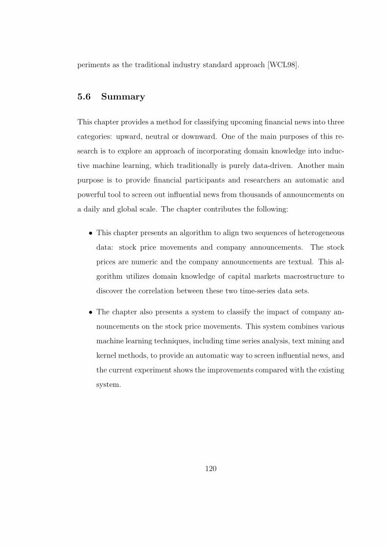
periments as the traditional industry standard approach [WCL98].
5.6 Summary
This chapter provides a method for classifying upcoming financial news into three
categories: upward, neutral or downward. One of the main purposes of this re-
search is to explore an approach of incorporating domain knowledge into induc-
tive machine learning, which traditionally is purely data-driven. Another main
purpose is to provide financial participants and researchers an automatic and
powerful tool to screen out influential news from thousands of announcements on
a daily and global scale. The chapter contributes the following:
• This chapter presents an algorithm to align two sequences of heterogeneous
data: stock price movements and company announcements. The stock
prices are numeric and the company announcements are textual. This al-
gorithm utilizes domain knowledge of capital markets macrostructure to
discover the correlation between these two time-series data sets.
• The chapter also presents a system to classify the impact of company an-
nouncements on the stock price movements. This system combines various
machine learning techniques, including time series analysis, text mining and
kernel methods, to provide an automatic way to screen influential news, and
the current experiment shows the improvements compared with the existing
system.
120

CHAPTER 6
Application II – Measuring Audit Quality
The Australia Stock Exchange (ASX) requires all of the publicly listed companies
to submit their accounting and auditing reports annually or biannually in order
to facilitate investors to estimate the performance of these companies. In this
chapter, two experiments are carried on data sets collected from these accounting
and auditing reports in order to estimate the quality of these auditing reports.
The first application in this chapter aims to discover publicly listed companies
with earning management behaviors. This is a challenge as earning management
behaviors typically do not follow a pattern and lead to the reports with poor
audit quality. This application is a binary classification task, and the companies
with illegal behaviors are classified as positive cases. These companies vary by
their industry categories (such as finance, transportation, retailer etc), sizes (such
as small, large, medium), and accounting conventions. These, and other, cate-
gories originate with related but not identical distributions rather than a single
identical one. It is inappropriate to directly group different types of companies
within a single category for the purpose of classification. Furthermore, the known
companies with earning management behaviors are rare among the public com-
panies of the ASX. For example, in 2003, only fourteen companies are reported
to have earning management behaviors among more than one thousand public
listed companies [BT05]. Thus the data set is extremely imbalanced. In the first
section of this chapter, the previously proposed VQSVM is employed to alleviate
121

the problems posed by this imbalanced audit and other data sets.
The second application utilizes characteristics of listed companies from the
ASX to estimate their audit fees. The audit fee is an important indicator of audit
quality. An abnormal audit fee (either higher or lower charge) regularly indicates
an audit report with a potential low quality. Audit researchers, Li and Stokes
have built a linear regression model with thirteen features to estimate audit fees
[LSH05]. This research examines a bigger data set and aims to discover more
features. Thus this application is a feature selection problem, and aims to extend
the original features of a linear model to other sets of features in a nonlinear
model.
6.1 VQSVM for Imbalanced Data
The class imbalance problem typically occurs when, in classification problems,
there are much more instances of some classes than others. In cases of extremely
imbalanced (or skewed) data sets with high dimensions, standard classifiers tend
to be overwhelmed by the large classes and ignore the small ones. Therefore,
machine learning becomes an extremely difficult task, and performances of regular
machine learning techniques decline dramatically. In practical applications, the
ratio of the small to the large classes can be drastic such as 1 to 100, or 1 to 1000
[CJK04].
Recent articles summarize some well-known methods for dealing with prob-
lems of imbalanced data, for example undersampling and oversampling at the
data level, one-class (cost-sensitive) learning and boosting at the algorithmic
level. Random undersampling potentially removes certain important examples,
and random oversampling leads to overfitting. In addition, oversampling intro-
122

duces additional computational costs if the data set is already fairly large but
imbalanced.
At the algorithmic level, cost-sensitive learning (chapter 3) aims to incorpo-
rate the risk factors of false positives and false negatives into the SVMs [VCC99]
[KS98] [LLW02]. Rehan Akbani et al implements the Synthetic Minority Over-
sampling TEchnique (SMOTE) to imbalanced data sets and discusses the draw-
backs of random undersampling. The SMOTE is a derivative of Support Vector
Machine that gives the different error costs for different classes to push the bound-
ary away from the minor class, [AKJ04]. Gang Wu et al implements KBA, Kernel
Boundary Alignment to imbalanced data sets [WC05].
There has been research in combining data compression and machine learning
techniques. Jiaqi Wang et al combines k-means clustering and SVM to speed up
real-time learning [WWZ05]. Scholkopf and Smola discusses the combination
between VQ and SVM in their book [SS02a]. They kernelized VQ as a new data
compression method, Kernel VQ. The modeling method proposed by this thesis
is different from their work as the VQSVM employs VQ to build a set of local
models whose outputs will be input to a global model (a SVM). One of major
applications of machine learning is data compression, so it is not surprising that
many works have been carried out in these two research fields.
Hierarchical learning machinery, VQSVM, is adapted to reduce the number of
instances within the major class by using less local models to represent instances
rather than simply eliminating instances randomly within random undersam-
pling. Because the local models inherit major information from the instances,
the information loss is much lower than the random undersampling. The local
models can retrieve the information from the global model. However, the local
models change the distribution of instances within the major class to some de-
123

gree, but according to the experiments the information loss caused by this change
is acceptable with respect to the improvement of overall performance.
6.1.1 Algorithms
The VQSVM is a hierarchical structure combining a set of local models that are
represented by codevectors and a global SVM. In some literature this type of
mixed model is named as semi-parametric model, because SVM is a well-known
nonparametric model and VQ is a parametric model with a rather transparent
structure. Semi-parametric hierarchical modelling thus becomes a way to incor-
porate domain knowledge into machine learning.
In the case of extreme imbalance datasets, the majority class is represented by
a set of local models that are codevectors, and the minority class keeps as original
observations. The local models can decode and retrieve original instances from
the codevectors. The number of local models in the majority is normally equal
to the number of observations in the minority. However, a tuning of the number
of the local models is required in order to reach the best performance.
Suppose the risk function of SVM is a hinge loss: R[f ] = 1m
∑mi=1 |f(xi) −
yi|. The risk function will receive a penalty if one observation is misclassified,
during the training process. In the imbalance data set, because the number
of observations in the major class is much more than the numbers in a minor
class, in the regular SVM, the penalties from the major class are often more
than those from the minor class. The larger portion of the penalties comes from
the major class. Thus the resultant hyperplane is pushed towards the minor
class, and causes misclassifications of some observations in the minor class. A
black point, representing an observation of minor class, is misclassified by the
regular SVM (see Figure 6.1). Rehan Akbani et al and Gang Wu et al also
124

Figure 6.1: After training, in an imbalanced and linearly nonseparable data set
the VQ replaces the original observations (light grey points) of the majority group
by codevectors (empty points). The number of the codevectors is almost equal to
the number of observations (dark grey points) of the minority group. The original
maximum margin hyperplane (middle grey areas with dashed lines) learned by
a soft margin SVM without the VQ is pushed towards a new position (middle
grey areas with solid lines), which is much closer to the majority group. The
previously misclassified observation (one dark grey point) is classified correctly
by the new hyperplane (middle grey areas with solid lines).
125

found that in the case of imbalanced dataset, SVM always pushes the hyperplane
towards a minority group. This hyperplane causes the learning machine to be
overwhelmed by the majority group, and the minority group loses its information
completely [AKJ04][WC05]. Cost-sensitive learning techniques, such as SMOTE,
function well as the higher weights of penalties are assigned to the minor class
by modifying the risk function [AKJ04].
On the small imbalanced data sets, an excessively reduced number of obser-
vations in the minority class contain very limited information and might not be
sufficient for learning. This is especially so when a large degree of class overlap-
ping exists and the classes are further divided into subclusters [TL05]. Japkowicz
performed several experiments on artificial data sets and concluded that class
imbalances do not seem to systematically cause performance degradation. She
concludes that the imbalance problem is a relative problem depending on both
the complexity of the concept and the overall size of the training set in addition to
the degree of class imbalance present in the data. The complexity of the concept
corresponds to the number of subclusters into which the classes are subdivided.
These results indicate that the class imbalance problems are very domain specific
instead of being caused only by the size of training data [Jap03]. Her work is
carried using the C4.5 decision tree, and as a quite different classifier, the SVM
is also sensitive to the class imbalance problem and it is worth testing whether a
similar idea is valuable.
The Support Vector Machine selects a set of vectors along the hyper-plane,
called support vectors. The random undersampling inevitably reduces the num-
ber of support vectors, and thus potentially loses information due to the removed
support vectors. According to the theory of data compression, vector quantiza-
tion is superior to random undersampling in terms of the information loss, but
126

both of them suffer from another risk of information loss within the majority
group. The SVM selects a subset of training instances, xi, and uses them as the
set of support vectors within the decision function shown in Equation 4.4. These
support vectors lie on the margin, and their coefficients αi are non-zero. In other
words, the hyperplane is completely determined by these support vectors, and
does not depend on other examples [SS02a]. Vector Quantization replaces the
original SVs by their corresponding codevectors. The codevectors become new
SVs and push the hyperplane away from the original place trained by imbalanced
data (see Figure 6.1). The Pseudo-code of the algorithm VQSVM is:
Algorithm 1 VQSVM algorithm
1: procedure VQSVM(dataset)
2: Float: g . the kernel parameter g
3: while Until The Optimal Point Of Tradeoff Between Information Loss
and Accuracy do
4: Int: numberOfLocalModels . the number of code-vectors
5: LocalModel = LBGvq(Majority, numberOfLocalModels)
6: NewTrainingData = combine(BalancedMajority, Minority)
7: Model = SVM(NewTrainingData, g)
8: end while
9: end procedure
VQSVM sacrifices the information held by the majority group to retrieve the
information contained by the minority group. This is very important in many real
life scenarios, which emphasize the minority groups. In this thesis, researchers in
the audit quality want to detect the rare annual reports with earning manage-
ments, but the majority of reports are without earning managements and are not
of interest. The number of local models is tuned by the VQSVM to minimize the
127

Data set Positive Negative Imbalance No. of number of
Insts Insts Ratio local models subclusters
Abalone (19) 32 4145 1:129.54 32 28
Audit 13 1271 1:98 16 ≥ 24
Yeast (5) 47 1437 1:30.5 64 8
Letter (26) 734 19266 1:26.28 299 (1024) 25
550 (2048) 25
Glass (7) 29 185 1:6.3 32 6
Table 6.1: Four UCI data sets and Audit data set with the numbers of local
models.
information loss of majority group. Therefore the optimal model is a trade-off
between the number of local models and the improved balance ratio in order to
improve the classification accuracy.
6.1.2 Experiments
Four University of California, Irvine (UCI) data sets and a data set collected by
Li and Stokes in the audit research are used for this evaluation [LSH05]. The
UCI data sets experimented with are abalone (abalone19), yeast (yeast5), glass
(glass7), and letter (letter26). The number in the parentheses indicates the target
class chosen. For example, the original glass data set contains 7 classes. In this
research, the seventh class is used as the minority side, and the other six classes
compound the majority side, so as to construct an imbalanced data set. Table
6.1 shows the characteristics of these six datasets organized according to their
negative-positive training-instance ratios. The top dataset (abalone19) is the
most imbalanced with a ratio of about 1 : 130. The abalone data set consists of
128

Figure 6.2: In the audit data set, the observations (the bigger points) of the
minority class is scattered with those (the smaller darker points) of the majority
class
continuous data instead of categorical data. It is expected that undersampling
at high rates generate a trade-off between improved data balance and loss of
important information. We examined whether different number of local models
could lead to a further enhancement of results. For example, in the letter(26)
data set, the experiments are carried out over two data sets with two various
number of local models (see Table 6.1).
Through the initial exploration of the five data sets, the minority class is not
linearly separated from the majority class. The minority class is scattered within
the majority class (see Figure 6.2).
The machine learning community uses two metrics, the sensitivity and the
specificity, for evaluating the performance of various tests. Sensitivity is defined
as the accuracy on positive instances,
Sensitivity =True Positives
True Positives + False Negatives
129

Specificity, however, is defined as the accuracy on negative instances [AKJ04]:
Specificity =True Negatives
True Negatives + False Positives
Kubat et al suggest the g-means, which combines specificity and sensitivity
[KM97]:
g =√
Specificity × Sensitivity
In our experiments, the g-means replace the standard accuracy rates, which do
not make any sense in imbalanced data sets.
In our experiments, we compare the performance of the modelling, VQSVM,
with the regular SVM, random undersampling and random oversampling [AKJ04].
The SVM uses the LibSVM code and the Vector Quantization uses the DCPR
Matlab toolbox [CL04][Jan05]. All tests involving the SVM use the RBF c-SVM
with an identical gamma value γ = 0.5 and an identical c value c = 10. Each
dataset is randomly split into training and test sets in the ratio 8 to 2, and only
the Abalone(19) is randomly split into train and test sets in the ratio 7 to 3,
because under the ratio 8 to 2, the experiments show that the Abalone (19) loses
the accuracy up to the g-mean value 0.1 with the random undersampling. For the
random undersampling algorithm, we undersample the training data until both
the classes were equal in number, as Japkowicz did in her experiments [Jap03].
The results of these experiments (see table 6.2) show that the g-means of the
VQSVM are better or equal to those of the standard SVM. This result prove
that the SVM is sensitive to the imbalanced data. In detail, the specificities of
the SVM are better than the VQSVM, but the SVM predicts all of instances
as negative. Thus the specificities of standard SVM do not make any sense. In
the data set, Letter (26), while the VQSVM sets the number of local models
extremely low, a new imbalanced data set is produced. As a consequence, the
130

SVM VQSVM
Data set Se Sp G Se Sp G
Abalone (19) 0 1 0 0.8 0.87623 0.83099
Audit 0 0.9948 0 0.2500 0.8583 0.4632
Yeast (5) 0 1 0 1 0.8606 0.9277
Letter (26) 0.3537 1 0.5948 1 0.1871 0.4326
0.7143 0.9992 0.8448
Glass (7) 0.6667 1 0.8165 0.6667 1 0.8165
Random Undersampling Random Oversampling
Data set Se Sp G Se Sp G
Abalone (19) 0.3000 0.8198 0.4959 0.6000 0.8101 0.6972
Audit 0.2750 0.6900 0.3653 0 1 0
Yeast (5) 0.8600 0.9519 0.9017 1 0.8084 0.8991
Letter (26) 1 0.0401 0.1998 0.4218 1 0.6494
0.7150 0.9993 0.8453 0.4218 1 0.6494
Glass (7) 0.8333 0.9757 0.8966 0.6667 1 0.8165
Table 6.2: Test Results: In the random undersampling, experiments are
carried out ten times for each data set. This reduces the error caused
by the random selection of observations. For example, in the data set
Yeast(5), we randomly withdrew 64 observations from original train data
10 times. The values in the table are the mean of the resultant g-mean
values. Under the VQSVM, the standard deviations of g-mean values are
0.1264(Abalone), 0.2600(Audit), 0.0612(yeast), 0.0013(Letter), 0.0758(glass)
131

predictive results of this data set show that the positive group overwhelms the
learning machine.
Compared with the results of random undersampling and oversampling, the
result of VQSVM is lower only when the number of local models in the majority
group is 299 in the data set “Letter (26)”. This is due to the over-reduction of
examples in the majority group. The tuning is essential to reach a trade-off be-
tween information loss and accuracy. According to the values of g-means in Table
6.2, in the data sets with low imbalance ratio (e.g. glass (7)), the performances of
three methods (random undersampling, oversampling and VQSVM) are almost
equally good, but in the data sets with high imbalance ratio (e.g. abalone (19)),
the performance of VQSVM is better than these of random undersampling and
oversampling.
6.1.3 Summary
The results of these experiments prove our theoretic hypothesis: the SVM is
highly sensitive to the imbalanced data, and majority groups often overwhelm
the learning machine. Similar to Gustavo Batista’s report, random oversampling
is more consistent than random undersampling in the case of the Support Vector
Machine. In the case of large amounts of training data containing imbalanced
classes, oversampling increases the number of training examples in the minority
classes, and therefore introduces more computation costs. Compared to three
other methods, the VQSVM is the most stable: from the abalone(19) with the
highest imbalance ratio 130 : 1 to the glass(7) with the lowest imbalance ratio
6 : 1, the g-mean values of the VQSVM hold at 0.8.
The results of these experiments coincide with the arguments Japkowicz pro-
posed [Jap03]. In the highly imbalanced data sets containing more subclusters,
132

the performance of the VQSVM is superior to the random undersampling. More
importantly, the VQSVM proposes a hierarchical structure, in which local models
can not be codevectors. The hierarchical structures give researchers more flexi-
bility to incorporate varying models representing domain knowledge into a mixed
model in dealing with imbalanced data sets.
Apart from the VQSVM, incorporating domain knowledge is always helpful
when addressing the problem of imbalance. With the Synthetic Minority Over-
sampling TEchnique (SMOTE), domain knowledge can be used to determine the
initial value of different error costs assigned to classes. This domain knowledge
helps overcome the sensitivity of inductive machine learning algorithms and then
produces more stable models. Instability means that arbitrarily small perturba-
tions in data sets can produce arbitrarily large perturbations in the solution. This
is especially true for infinite-dimensional problems, because for finite-dimensional
problems that perturbation is always finite. But the key of this problem is that
the solution to the new problem is less sensitive to the perturbations [Han05].
Most non-parametric methods, such as SVM, provide ways to stabilize and
regularize the problem. However, their regularization (See Section 2.1.3) is often
a global solution, which assumes that the underlying distribution is identical.
If the underlying distribution is not identical, it becomes highly risky to make
these assumptions, and causes instabilities of the resultant model. In contrast,
hierarchical modelling practises alternative approaches, that separates the related
distributions first, building a local model over each sub-region, and then unifying
local models via a nonparametric model. From the experiments, the VQSVM
overcomes the sensitivity created due to the imbalance suffered by the SVM. With
balanced data, the performance of the VQSVM is equivalent to the performances
of SVM. In the case of extremely imbalanced data, VQSVM reaches an acceptable
133

level of accuracy while SVM is already overwhelmed by the majority groups.
6.2 Feature Selections
Chapter 4 discusses the basic concepts of relevant and redundant features, and the
measurement of mutual information between features. Based on these discussions,
this section proposes a feature selection algorithm for the SVM and tests it over
the same audit data set as the one used in the previous experiment of the VQSVM.
6.2.1 Algorithms
The proposed algorithm assembles the previous discussion in chapter 4, and con-
sists of three major steps. The first step is a grid search which repeats the KCCA
between feature candidates until the results are consistent with the ML and MP
constraints. The second step consists of a feature ranking by using a Recur-
sive Feature Elimination (RFE) SVM proposed by Guyon el at [GWB02]. The
RFE is a kernel-based backwards feature selection method. With every iteration,
it eliminates one or multiple features, testing the impact of elimination on the
model coefficients learned by the SVM. If the impact of one removal feature is
minimal among the candidates, it has the least influence in the resultant model.
The output of the RFE is a list of ordered features. The order is determined
by the influence of the features. For example, on the descending list, the most
influential feature is the first one on the list.
The third step follows Lei Yu and Huan Liu’s Fast Correlation-Based Filter
(FCBF) to remove the redundant features based on the results from the previous
two steps [YL04]. In the case of a descending list, a search starts from the
beginning of the list. Suppose a feature Fj precedes another feature Fi; if the
134

Figure 6.3: The measurements in the FCBF algorithm proposed by Lei Yu and
Huan Liu [YL04]
correlation coefficient SUi,j between Fj and Fi is greater than the correlation
coefficient Ri,c between Fi and the target T , the feature Fi is removed from the
list (see Figure 6.3). The search carries on until the end of the list, the result
being an optimal subset of features.
In this algorithm proposed by the author, prior knowledge in the format
of known relevant features is represented as two types of constraints: 1) a set
of must-link constraints ML(Fi, T ) between the target T and each of known
relevant features Fi ∈ Sknown, and 2) a set of must-precede constraints MP (Fi, Fj)
between known relevant features, where Corr(Fi, T ) ≥ Corr(Fj, T ) and Fi, Fj ∈Sknown. These constraints play a crucial role in directly determining the accuracy
of the measurement of KCCA. For example, if the RBF is employed as the kernel
functions, the grid search aims to detect the optimal value of the coefficient γ in
the RBF k(xi, xj) = e−γ‖xi−xj‖2 . The coefficient γ determines mapping between
the input space and the feature space. The pseudo code of the algorithm is
outlined below:
135

Algorithm 2 Feature Selection Algorithm
1: procedure FeatureSelection(S(F1, F2, ..., FN , T ),ML,MP, δ)
. S is a training data set; δ is a predefined threshold; ML: the set of
must-link constraints; MP : the set of must-precede constraint.
2: S ′list=FeatureRanking(S)
3: while (∀SUi ∈ SU)SUi ° ML, MP do
4: SU= GridSearch(KCCA(S, Sknown))
5: end while
6: Fj = getFirstElement(S ′list)
7: while Fj 6= NULL do
8: Fi = getNextElement(S ′list, Fj)
9: while Fi 6= NULL do
10: if SUi,j > Ri,c then
11: remove Fi from S ′list
12: end if
13: Fi=getNextElement(S ′list, Fi)
14: end while
15: Fj=getNextElement(S ′list ,Fj)
16: end while
17: Sbest=S ′list
18: return Sbest
19: end procedure
In the following sections, this algorithm is tested over an artificial data set
and a real-world data set which is collected from the audit quality research.
136
0 5 10 15 20 25 300.25
0.3
0.35
0.4
0.45
0.5
0.55
0.6
0.65
0.7
Figure 6.4: The test accuracy of models constructed by a SVR while eliminating
one feature every iteration. The x-axis is the index of feature in the ascending
list, and the y-axis is the R-square.
6.2.2 Experiments
First, the author modifies a data generation provided by Leo Breiman [Bre96b]
to produce an artificial data set. The artificial data set consists of 30 features and
60 pairs of observations. The modification is: within ten features, assign the 0.2
time of the value of fifth feature to the fourth feature, F4 = 0.2F5, F14 = 0.2F15
and F24 = 0.2F25. Thus, among the thirty features of this artificial data set,
there are six weak relevant features, three strong relevant features and twenty-
one irrelevant features. The index of weak relevant features is 4, 14, 24, 5, 15,
25 and the index of strong relevant features is 6, 16, 26. The Recursive Feature
Elimination (RFE) SVM produces a list of ranked features and the values of
R-square while eliminating one feature every iteration (See Figure 6.4). The
resultant list of ranked features is 2, 1, 18, 30, 29, 13, 20, 19, 11, 12, 8, 23, 21, 7,
10, 3, 9, 22, 17, 6, 14, 4, 24, 28, 27, 26, 5, 16, 25, 15. In the Figure 6.4, at the flat
top part of the curve, the weak relevant features and strong relevant features mix
137

Sigma σ Ranked features
10 2, 1, 18, 30, 29, 13, 20, 19, 11, 12, 8, 23, 21, 7, 10, 3,
9, 22, 17, 6, 14, 4, 24, 28, 27, 26, 5, 16, 25, 151 2, 7, 25, 9, 15, 13, 1, 23, 6, 5, 21, 30, 16, 17, 8, 29, 19,
11, 22, 12, 20, 18, 3, 28, 10, 27, 26, 24, 14
Table 6.3: The RBF SVM with the different values of sigma produces different
lists of ranked features. The lists are ordered from the least important to the
most important.
with a few irrelevant features. It is difficult for the backward sequential feature
selection to discover the redundant features from the weak redundant features
and then uncover the optimal subset of features.
However, by taking account of the mutual information between feature can-
didates, the proposed feature selection discovers the strong correlation between
feature candidates. At the same time, the correlation between the 5th feature
and the target is larger than the correlation between the 4th feature and the
target. Therefore the optimal subset of feature produced by the proposed feature
selection algorithm includes the features 6, 28, 27, 26, 5, 16, 25, 15. The mean
R-square of 10 times cross-validation of a SVR with the same hyper-parameter
as the previous SVRs is 0.689527. That is close to the best R-square value of the
previous backwards sequential feature selection.
At the same time, different values of the hyper-parameter, such as the sigma
in the RBF kernel, may produce different lists of ranked feature. The previous list
is produced while the sigma is 10. When the sigma is set to be 1, the resultant
list becomes 2, 7, 25, 9, 15, 13, 1, 23, 6, 5, 21, 30, 16, 17, 8, 29, 19, 11, 22,
12, 20, 18, 3, 28, 10, 27, 26, 24, 14 (See comparison in Table 6.3). The same
138
as other kernel based algorithms, the RBF SVM and Kernel CCA are sensitive
to the value of hyper-parameters. The selection of hyper-parameters can benefit
from the known domain knowledge. If the 6th features are known to be strong
relevance, the second list can be discarded as compared with the first list. Their
sensitivity is caused by the fact that kernel based algorithms are approximate to
the underlying relations. The accuracy of the approximation is heavily influenced
by the value of hyper-parameters and noise within the features and observations.
Secondly, a real-world data set is employed to test the proposed feature selec-
tion algorithm. The data set is the auditing and accounting reports from listed
companies in the Australian Stock Exchange (ASX) in 2003. To ensure an ap-
propriate data set for the experiments, we first need to exam whether the data
set contains both relevant and redundant features. The RFE SVM produces an
ascending list of 39 ranked features (more important features are close to the
end): 35, 30, 29, 34, 33, 32, 17, 1, 18, 4, 8, 31, 14, 36, 37, 10, 13, 15, 3, 25, 12,
28, 24, 26, 22, 27, 16, 20, 21,11, 2, 23, 38, 7, 9, 6, 19, 5, 39. The same as previ-
ous experiment, Figure 6.5 demonstrates the test result of nonlinear Radial Basis
Function Support Vector Regression (RBF SVR), with each iteration removing
one feature. The order of feature removal follows the order of feature-ranking
list. The flat middle part of the curve indicates that the eliminated features do
not have strong impacts on the test accuracy of the resultant model, and this
result indicates the existence of redundant features.
According to the proposed algorithm, the Kernel CCA is employed to mea-
sure the correlation coefficients between features. If the correlation coefficient
between features is greater than 0.05 (KCCA > 0.05), the coefficient is retained
in the final KCCA table. Otherwise, this experiment sets two of the correspond-
ing features as irrelevant. In the final KCCA table, the index of the features
139

Figure 6.5: The test accuracy of SVR models while eliminating one feature every
iteration. The x-axis is the index of feature in the ascending list, and the y-axis
is the value of R-square.
without strong correlations to the known relevant features is (10, 14, 25, 29-32,
36-37). Based on these results, the proposed algorithm generates an optimal
subset of features consisting of 16 features: Loss Indicator (1), YE (8), OFOA
(31), Current Liabilities (14), 12 Months (36), Currency (37), Current Assets
(10), DE (3), QUICK (2), AF/EBIT (38), CATA (7), FOREIGN (9), LnSUB(6),
Partner Code (19), LnTA (5), AF/TA (39). Using the SVR with 100 random
sampling 80% of the original data set as the training data, the average test result
(R-square) is 0.8033 with the standard deviation 0.0398. This result is slightly
higher than 0.774, the best test result (R-square) using the SVR with the same
hyper-parameters but the subset of features produced by the backwards feature
sequential selection.
140
6.2.3 Summary
This research expands Lei Yu and Huan Liu’s Fast Correlation-Based Filter
(FCBF) [YL04]. It does so primarily in that it implements the redundancy mea-
surement in feature selection for the non-linear regression. As domain knowledge,
known relevant features are included in the process to guide the process of the
KCCA, under the condition that a sufficient amount of known relevant features is
available. Considering the human involvement, it is worth ensuring whether the
KCCA produces an appropriate approximation to the real mutual information.
In this research, however, domain knowledge from experts is utilized to guide
tuning of the parameters of selected kernels.
In the feature selection experiment of this thesis, domain knowledge collected
from domain experts’ past experiments is included to set the width of the kernel.
According to the results of the experiments, the different values of the hyper-
parameters produce very different outcomes. This is due to the fact that the
kernel based algorithms are approximate to the unknown relations. The domain
knowledge plays an important role to guide the search process to discover the
relatively correct setting. Other researchers often employ the grid search to dis-
cover the optimal value [SBK04]. In the case of this thesis, the domain knowledge
facilitates this process.
The results of these experiments show that the optimal set of features increases
the accuracy to a relatively high level with relatively small optimal subset of fea-
tures. A similar idea can be found in Carlos Soares et al’s meta-learning methods
to select kernel width in SVR [SBK04]. Their meta-learning methodology exploits
information about past experiments to set the width of the Gaussian kernel. At
this stage, the result still relies heavily on the given domain knowledge with the
assumption that the given domain knowledge is perfect. The most pertinent area
141

for further investigation is the negative impacts of given domain knowledge on
the resultant subset of features.
142

CHAPTER 7
Conclusion and Future Works
7.1 Brief Review and Contributions of this Thesis
In this thesis, a framework and methods are proposed that incorporate prior do-
main knowledge into inductive machine learning. Chapter 2 briefly introduces
the basic concepts of both inductive machine learning and domain knowledge.
Chapter 3 follows by showing that domain knowledge can be incorporated into
inductive machine learning through three key issues: consistency, generalization
and convergence. These three issues are not separate from each other, but are
addressed simultaneously by the majority of methods. In addition, existing re-
search on this topic has been categorized and analyzed according to the previously
proposed three key issues.
In chapter 4, three new methods incorporating domain knowledge into ker-
nel methods are proposed. The first method employs logical clauses to label the
unlabeled training data for supervised learning algorithms. The second method,
VQSVM, consists of vector quantization and a Support Vector Machine (SVM)
to construct a semi-parametric hierarchical model. In the VQSVM, the VQ con-
structs and represents the local models and the SVM acts as a global model.
The third method employs domain knowledge as sets of constraints to guide the
parameter selection of the KCCA.
In chapter 5, the proposed first method, domain knowledge in the format
143

of logical clause, is applied to the measurement of unexpected news on stock
price movements. A set of logical clauses combines discoveries made by piecewise
linear fitting and volatility analysis over a data set consisting of the half-hourly
Volume Weighted Average Prices (VWAP) to label the company announcements.
The resultant labeled training examples are then fed into an SVM for supervised
learning.
In chapter 6, the proposed second method, VQSVM, is tested over several
imbalanced data sets, including an auditing data set. The results show that the
VQSVM is superior in terms of classification performance and stability to the
current methods dealing with imbalanced data. The proposed third method is a
kernel-based feature selection algorithm expanding the existing algorithm to the
problem of nonlinear regression. The experiment over the audit data set shows
that the proposed algorithm elicits an optimal subset of features and improves
the estimation performance.
Overall, this thesis makes three major contributions. First, it raises a problem
often ignored by machine learning communities, especially academic researchers:
how domain knowledge can be incorporated into inductive machine learning in
order to enhance the performance of existing complex systems. Secondly, it pro-
poses a framework of incorporating domain knowledge into inductive machine
learning regarding three key issues of inductive machine learning: consistency,
generalization and convergence. Within this framework, it is rather straightfor-
ward for inductive machine learning algorithms to include domain knowledge.
Thirdly, this thesis presents three new methods of incorporating domain knowl-
edge into inductive machine learning. These methods give users the flexibility to
allow their expertise to be included in some formats. It is essential to consider the
negative impacts of domain knowledge, while using imperfect domain knowledge
144

to diminish the negative impacts from imperfect training data; even the training
data conflicting with imperfect domain knowledge. From the experiments and
ensuing discussion, the benefits of incorporating prior domain knowledge can be
summarized in three major aspects: 1) reducing the requirements to the quality
and quantity of training examples without sacrificing of the performance of the
learning system; 2) quick deployment and efficient adaption to dynamic environ-
ments; and 3) more transparent outputs of the learning system helping users gain
a deeper understanding of the resultant model.
7.2 Future Research
This research provides some approaches to utilizing prior domain knowledge as
an auxiliary information source in addition to the observations to enhance the
abilities of learning algorithms in certain domains. Although this sounds straight-
forward, it is difficult to realize the correct utilization in many inductive learning
algorithms due to their complexity and the variety of domain knowledge. Avail-
able research as yet has not produced a universal solution to this topic. The
main difficulties of incorporating prior domain knowledge into inductive machine
learning come from several points:
1. The difficulty of collecting domain knowledge:
The main plausible source of collecting domain knowledge until recently
has been human domain experts. When building knowledge representa-
tions from human experts, machine learning practitioners must elicit the
knowledge from human experts via interviewing or testing so as to discover
compact representations of their understanding. This encounters a num-
ber of difficulties, which collectively make up the ”knowledge bottleneck”
145
[KN04]. With many large-scale databases a limited amount of prior domain
knowledge exists; in many cases there simply is no expert to interview, such
as with business confidential knowledge in many financial industries. In
other cases it is difficult to articulate the humans’ expertise, as much of it
relies on personal experience.
2. Imperfection (or uncertainty) of domain knowledge:
It is extremely rare that domain knowledge is perfect, accurate and com-
prehensive. The imperfection comes from the collection process of domain
knowledge, such as interviews with human experts and the formalization of
that knowledge. Misunderstandings, or obstacles of understanding, often
occur between machine learning researchers and domain experts.
3. The difficulty of representing domain knowledge in learning algorithms :
The majority of inductive learning algorithms only deal with numerical
data. It is relatively easy if domain knowledge can be represented in formats
of numerical data, such as virtual samples. However, there is a significant
portion of domain knowledge that is difficult to be transformed into numer-
ical data, as further research is then necessary for the domain knowledge to
be valuable for learning. The difficulties of representation also come from
that domain knowledge not being well structured or defined.
4. The difficulty of balancing the effects from domain knowledge and observa-
tions :
The difficulty of balancing the effects from domain knowledge and obser-
vations happens when there are conflicts between domain knowledge and
observations. Some algorithms balance their effects by a Lagrange Multi-
plier. In that case, domain knowledge is treated as a set of constraints, and
146

the violations to the constraints are punished to some degree. However in
many cases, domain knowledge cannot be included in a Lagrange function.
This research mainly addresses the last difficulties 2,3, and 4. The results have
demonstrated that it is of great benefit to inductive machine learning to incor-
porate domain knowledge in its learning process. In regards to these difficulties,
the explorations in this research can be improved in some possible aspects.
Firstly, a deeper investigation into the relationship between true risk R and
the combination of empirical risk and domain knowledge risk Remp + Rknowledge
is needed. In theory, the combination of empirical risk and domain knowledge
Remp + Rknowledge can provide a more tight bound for the true risk: |[Remp(f) +
Rknowledge(f)] − R(f)| < δ, similar to the structure risk. Generally, overfitting
causes a bigger domain knowledge risk Rknowledge and a smaller empirical risk
Remp. However, there is not as yet a general method to qualify this tighter
bound.
Secondly, in hierarchical modelling, a further study could aim to address the
trade-off between local and global models regarding conflicts. For example, a
global model initiates new local models based on current local models. However
the typical resultant local model is not coherent to the given training examples.
A related problem exists in how to uncover the optimal point for partitioning
observations and features in order to improve the generalization of the global
model without losing the accuracy of the local models.
The current results of the experiments show a significant improvement in
binary classification. In further works, it is necessary to investigate more precise
controls. Especially the local models representing only support vectors instead
of all vectors may enhance the controllability of the VQSVM and manage the
information loss that occurs with VQSVM.
147

There is one issue the VQSVM is unable to address: the size of the training
data. This phonomania has been observed in the experiment over the data set
“Audit”. If the size of the training data, or more precisely, the size of minor class
is extremely small, the information contained will be too limited to be learned
by the VQSVM, thus degrading its performance.
Thirdly, in the feature selection problem, it is still arguable as to what degree
the algorithm needs to successfully rely on domain knowledge. In the experi-
ments of this thesis, the algorithm relies fully on the sufficient domain knowledge
available. It is worthwhile expanding the algorithm into the domain without
enough knowledge and analyze the results. Some sensitivity analysis is necessary
to explore how sensitive the parameter setting is to domain knowledge and how
the parameters setting affects the performance of the feature selection algorithm,
although there is an initial exploration to this issue in Chapter 6.
Fourthly, in the logical representation of domain knowledge in inductive ma-
chine learning, there is still a huge gap between domain experts and machine
learning practitioners. This thesis provides an example demonstrating the use-
fulness of domain knowledge in the forms of logical clauses within learning sys-
tems. However the solution is still domain-dependent, and requires the users’
involvement with the domain to design similar approaches.
The current prototype has demonstrated promising results of this approach.
Further work is needed to provide prototypes that can analyze the impact of
news on stock prices in a more complex and real environment. Due to the lack
of data, the experience in this thesis only is carried over a data set, and may be
affected by the characteristics of the data set. In the further work, the similar
experiments need to be carried over various data sets to test the robustness of
the proposed method. In addition, in further work, three major issues remain,
148

as suggested by Nikolaus Hautsch:
1. Impact of the disclosure of inside information: If inside information has
been disclosed at the market even before the announcement, the price dis-
covery process will be different.
2. Anticipated vs. unanticipated information: If traders’ belief has absorbed
the anticipated information, the impact must be expressed as a conditional
probability with the belief as a prior condition. A potential source of
traders’ belief is the database called the Institutional Brokers Estimate
System (I/B/E/S).
3. Interactive effects between information: The current experiment posits that
all news at one point is labelled as a set of upward impacts, but a real
situation is much more complex. Even at one upward point, it is common
that there exists news with downward impacts. It will be very challenging
to distinguish the subset of minor news and measure the interrelationship
between all available news [HH05].
To fulfill the suggested further works, more data including the information of
traders’ current brief is crucial. Incorporating deeper domain knowledge regard-
ing the interrelationship between stock price movements and news arrivals will
be beneficial. Moreover, other domain knowledge is required to tailor the rule
base and the corresponding time-series techniques, if the method of alignment is
implemented in other environments.
Finally, there is still no general solution to incorporating prior domain knowl-
edge into inductive machine learning due to the four main difficulties. At this
stage, even though many researches already make the required assistances to be
149

less, if one incorporates their own expertise into an inductive machine learning
algorithm, assistance from the machine learning practitioner remains essential.
In order to solve this topic eventually, the most essential problem is to discover
a method that can represent various domain knowledge easily and clearly into
inductive learning machines. Sometimes it is more critical to give a fine definition
of a problem before solving it. This thesis has identified and tested a framework
and three new methods of incorporating prior domain knowledge into inductive
machine learning. The future research paths proposed in this final chapter show
a way towards finding a solution.
150

APPENDIX A
Abbreviation
ABS – Adaptive Belief System
ANN – Artificial Neural Network
ASX – Australian Stock Exchange
CCA – Canonical Correlation Analysis
EBL – Explanation-Based Learning
EBNN – Explanation-Based Neural Network
FCBF – Fast Correlation-Based Filter
FOL – First-Order Logic
ICA – Independent Component Analysis
KBANN – Knowledge-Based Artificial Neural Network
KCCA – Kernel CCA
KKT Condition – Karush-Kuhn-Tucker Condition
KSVM – Knowledge-based Support Vector Machine
LBG-VQ – Linde, Buzo, Gray - Vector Quantization
MDL – Minimum Description Length
ML – Must-Link
MP – Must-Precede
151

OOBNs – Object Oriented Bayesian Networks
PAC-learnable – Probably Approximately Correct-learnable
PCA – Principle Component Analysis
RBF – Radial Basis Function
REH – Rational Expectations Hypothesis
RFE – Recursive Feature Elimination
RKHS – Reproducing Kernel Hilbert Space
SMO – Sequential Minimal Optimization
SMOTE – Synthetic Minority Over-sampling TEchnique
SRM – Structural Risk Minimization
SV – Support Vector
SVM – Support Vector Machine
SVR – Support Vector Regression
TF-IDF – Term Frequency - Inverse Document Frequency
VC dimensions – Vapnik Chervonenkis dimensions
VQ – Vector Quantization
VQSVM – Vector Quantization Support Vector Machine
VWAP – Volume Weighted Average Prices
WMSVM – Weighted Margin Support Vector Machine
152

APPENDIX B
Table of Symbols
〈., .〉 – Inner Product
‖ . ‖ – Norm
(xi, yi) – A training data pair as i is the index
c(x) – Unknown Target Function
Corr(., .) – Correlation Coefficient
inf(.) – Inferior, that is the best lower bound
k(., .) – kernel function
RN – N-dimensional Euclidean space
R(f) – Risk Function (or loss function, error function)
Remp(f) – Empirical Risk Function
R(fn) – Risk function of any function fn within the given hypothesis space
R(fH) – Risk function of the best function within the given hypothesis space H.
sgn(.) – Sign
sup(.) – Superior, that is the best upper bound
153

References
[AB99] M Anthony and P. Bartlett. Neural Network Learning: TheoreticalFoundations, chapter 5. Cambridge University Press, 1999.
[ABH95] Sarabjot S. Anand, David A. Bell, and John G. Hughes. “The roleof domain knowledge in data mining.” In Proceedings of the fourthinternational conference on information and knowledge management,pp. 37 – 43, Baltimore, Maryland, United States, 1995. ACM PressNew York, NY, USA.
[Abu95] Yaser. S. Abu-Mostafa. “Hints.” Neural Computation, 7:639–671,1995.
[Abu01] Yaser. S. Abu-Mostafa. “Financial model calibration using consistencyhints.” IEEE Trans. on Neural Networks, 12(4):791–808, July 2001.
[AHU74] Alfred V. Aho, John E. Hopcroft, and Jeffrey D. Ullman. The de-sign and analysis of computer algorithms, chapter 10. NP-CompleteProblems. Addison-Wesley series in computer science and informa-tion processing. Addison-Wesley, 1974.
[AKJ04] Rehan Akbani, Stephen Kwek, and Nathalie Japkowicz. “ApplyingSupport Vector Machines to Imbalanced Datasets.” In Proceedingsof the 15th European Conference on Machine Learning (ECML), pp.39–50, 2004.
[Alp04] Ethem Alpaydin. Introduction to Machine Learning. The MIT Press,2004.
[Bax00] Jonathan Baxter. “A Model of Inductive Bias Learning.” Journal ofArtificial Intelligence Research, 12:149–198, 2000.
[BBL04] Oliver Bousquet, Stephane Boucheron, and Gabor Lugost. “Introduc-tion to Statistical Learning Theory.” In Advanced Lectures on MachineLearning Lecture Notes in Artificial Intelligence 3176, pp. 169–207.Springer, Heidelberg, Germany, 2004.
[BH02] Michael Berthold and David J. Hand. Intelligent Data Analysis, AnIntroduction 2nd Edition. Springer, 2002.
[BJ02] Francis R Bach and Michael I Jordan. “Kernel Independent Compo-nent Analysis.” Journal of Machine Learning Research, 3:1–48, 2002.
154

[Bre96a] Leo Breiman. “Bias, variance, and arcing classfiers. Tech Rep 460.”Technical report, Statistics Dept. U. of California, Berkeley, April1996.
[Bre96b] Leo Breiman. “Heuristics of Instability and Stabilization in ModelSelection.” The Annals of Statistics, 24(6):2350–2383, 1996.
[BS97] Christopher J.C. Burges and Bernhard Scholkopf. “Improving theaccuracy and speed of support vector learning machine.” Advances inNeural Information Processing System, 9:375–381, 1997.
[BT05] Philip Brown and Ann Tarca. “Achieving high quality, comparablefinancial reporting: A comparison of independent enforcement bodiesin Australia and the United Kingdom.” 2005.
[CA92] Fred Collopy and J Scott Armstrong. “Rule-Based Forecasting: De-velopment and Validation of an Expert Systems Approach to Com-bining Time Series Extrapolations.” Journal of Management Science,38(10):1394–1414, 1992.
[CJ05] Carole Comerton-Forde and Elvis Jarnecic. “Introduction to MarketMicrostructure, Capital Markets Co-operative Research Centre.” Lec-ture Notes, September 2005.
[CJK04] Nitesh V. Chawla, Nathalie Japkowics, and Aleksander Kolcz. “Edi-torial: special issue on learning from imbalanced data sets.” SIGKDDExplorations, 6(1), 2004.
[CL96] B.P. Carlin and T.A. Louis. Bayes and Empirical Bayes Methods forData Analysis. Chapman and Hall, 1996.
[CL01] C. Chang and C. Lin. “LIBSVM: a library for support vector ma-chines (version 2.3).” Technical report, The National Taiwan Univer-sity, 2001.
[CL04] Chih-Chung Chang and Chih-Jen Lin. “LIBSVM: a Library for Sup-port Vector Machine.” Technical report, Department of Computer Si-cence and Information Engineering, National Taiwan University, 2004.
[CLM97] John Y. Campbell, Andrew W. Lo, and A. Craig MacKinlay. TheEconometrics of Financial Markets. Princeton University Press, 1997.
[CS96] Peter Cheeseman and John Stutz. “Bayesian Classification (Auto-Class): Theory and Results.” In Advances in Knowledge Discoveryand Data Mining, pp. 153–180. 1996.
155

[CT03] L. J. Cao and Francis E. H. Tay. “Support Vector Machine withAdaptive Parameters in Financial Time Series Forecasting.” On theIEEE Transaction on Neural Networks, 14(6), 2003.
[DCT04] Robert Dale, Rafael Calvo, and Marc Tilbrook. “Key Element Sum-marisation: Extracting Information from Company Announcements.”In Proceedings of the 17th Australian Joint Conference on ArtificialIntelligence, Cairns, Queensland, Australia, 2004.
[DLM03] Richard Dybowski, Kathryn B. Laskey, James W. Myers, and SimonParsons. “Introduction to the Special Issue on the Fusion of DomainKnowledge with Data for Decision Support.” Journal of MachineLearning Research, Fusion of Domain Knowledge with Data forDecision Support:293–294, 2003.
[DR05] Ian Davidson and S. S Ravi. “Hierarchical Clustering with Con-straints: Theory and Practice.” In the 9th European Principles andPractice of KDD, PKDD, 2005.
[DS02] Dennis Decoste and Bernhard Scholkopf. “Training Invariant SupportVector Machines.” Machine Learning, 46:161–190, 2002.
[FMS01] Glenn M Fung, Olvi L Mangasarian, and Jude W Shavlik.“Knowledge-Based Support Vector Machine.” Technical report, DataMining Institute, Computer Science Department, University of Wis-consin, Madison, 2001.
[FPS96] U.M. Fayyad, Piatesky-Shapiro, and G. Smyth, editors. Advances inKnowledge Discovery and Data Mining. AAAI Press and The MITPress, 1996.
[FS95] Y. Freund and R.E. Shapire. “A decision theoretic generalization onon-line learning and an application to boosting.” In ComputationalLearning Theory. 2nd European Conference, pp. 23–27, 1995.
[Fyf92] William John Andrew Fyfe. Invariance Hints and the VC Dimension.PhD thesis, 1992.
[GG92] Allen Gersho and Robert M. Gray. Vector Quantization And SignalCompression. Kluwer Academic Publishers, 1992.
[GH96] Saul I. Gass and Carl M. Harris. Encyclopedia of operations researchand management science. Boston : Kluwer Academic Publishers,1996.
156

[Gha04] Zoubin Ghahramani. “Unsupervised Learning.” In Olivier Bousquet,Ulrike von Luxburg, and Gunnar Ratsch, editors, Advanced LecturesOn Machine Learning: ML Summer Schools 2003, Canberra, Aus-tralia, 2-14, 2003, Tbingen, Germany, August 4-16, 2003 : revisedlectures, pp. 72–112. Springer, 2004.
[Gio02] Fabio Roli Giorgio Fumera. “Cost-sensitive learning in Support VectorMachines.” 2002.
[GS99] Valery Guralnik and Jaideep Srivastava. “Event Detection From TimeSeries Data.” In KDD-99, San Diego, CA USA, 1999.
[GT00] J. Galindo and P. Tamayo. “Credit Risk Assessment Using Statis-tical and Machine Learning: Basic Methodology and Risk ModelingApplications.” Computational Economics, 15(1-2):107 – 143, 2000.
[GWB02] Isabelle Guyon, Jason Weston, Stephen Barnhill, and Vladimir Vap-nik. “Gene Selection for Cancer Classification using Support VectorMachines.” Machine Learning, 46(1-3):389 – 422, 2002.
[Hal99] Mark A. Hall. Correlation-based Feature Selection for Machine Learn-ing. Phd thesis, Waikato University, 1999.
[Han05] Per Christian Hansen. “Discrete Inverse Problems, Insight and Algo-rithms, A tutorial with Matlab exercises.” Technical report, Informat-ics and Mathematical Modelling Building 321, Technical University ofDenmark DK-2800 Lyngby, Denmark, November 2005.
[HH05] Nikolaus Hautsch and Dieter Hess. “Bayesian Learning in FinancialMarkets - Testing for the Relevance of Information Precision in PriceDiscovery.” Journal of Financial and Quantitative Analysis, 2005.
[Hom01] Cars H. Hommes. “Financial Markets as Nonlinear Adaptive Evolu-tionary Systems.” Technical report, University of Amsterdam, 2001.
[Jan05] Jyh-Shing Roger Jang. “DCPR MATLAB Toolbox.”, 2005.
[Jap03] Nathalie Japkowicz. “Class Imbalances: Are We Focusing on the RightIssue?” In Workshop on Learning From Imbalanced Data Sets II, 2003.
[JKP94] George H. John, Ron Kohavi, and Karl Pfleger. “Irrelevant Featuresand the Subset Selection Problem.” In The International Conferenceon Machine Learning, pp. 121–129, 1994.
157

[JS99] Yaoch Jin and B. Sendhoff. “Knowledge incorporation into neuralnetworks from fuzzy rules.” Neural Processing Letters, 10(3):231–242, 1999.
[JW01] Richard A. Johnson and Dean W. Wichern. Applied Multivariate Sta-tistical Analysis. Prentice Hall, 4th edition, 2001.
[JYD04] Tony Jan, Ting Yu, John Debenham, and Simeon Simoff. “Finan-cial Prediction using Modified Probabilistic Learning Network withEmbedded Local Linear Models.” In CIMSA2004-IEEE InternationalConference on Computational Intelligence for Measurement Systemsand Applications, Boston, MD, USA, 2004.
[KCH01] Eamonn Keogh, Selina Chu, David Hart, and Michael Pazzani. “AnOnline Algorithm for Segmenting Time Series.” In In Proceedings ofIEEE International Conference on Data Mining, pp. 289–296, 2001.
[KCH03] Eamonn Keogh, Selina Chu, David Hart, and Michael Pazzani. “Seg-menting Time Series: A Survey and Novel Approach.” In Data Miningin Time Series Databases. World Scientific Publishing Company, 2003.
[Key36] John Maynard Keynes. The General Theory of Employment, Interestand Money. Harcourt, Brace and World, 1936.
[KM97] Miroslav Kubat and S Matwin. “Addressing the Curse of ImbalancedData Sets: One-Sided Sampling.” In Proceedings of the FourteenthInternational Conference on Machine Learning, pp. 179–186, 1997.
[KN04] Kevin B. Korb and Ann E. Nicholson. Baysian Artificial Intelligence.Chapman & Hall/CRC, 2004.
[KS96] Daphne Koller and Mehran Sahami. “Toward Optimal Feature Selec-tion.” In the Thirteenth International Conference on Machine Learn-ing, pp. 284–292. Morgan Kaufmann, 1996.
[KS98] Grigoris Karakoulas and John Shawe-Taylor. “Optimizing classifiersfor imbalanced training sets.” In Advances in neural information pro-cessing systems, pp. 253 – 259. MIT Press, Cambridge, MA, USA,1998.
[KSB01] S. Keerthi, S. Shevade, C. Bhattacharyya, and K. Murthy. “Improve-ments to Platt’s SMO algorithm for SVM classifier design.” NeuralComputation, 13:637–649, 2001.
158

[KV00] Boris Kovalerchuk and Evgenii Vityaev. Data Mining in Finance:Advances in Relational and Hybrid Methods. Kluwer Academic Pub-lishers, 2000.
[KVY02] Boris Kovalerchuk, Evgenii Vityaev, and Husan Yusupov. “SymbolicMethodology in Numeric Data Mining: Relational Techniques for Fi-nancial Applications.” In arXiv.org: Computational Engineering, Fi-nance, and Science, cs.CE/0208022, 2002.
[LB03] David E. Losada and Alvaro Barreiro. “Embedding term similarityand inverse document frequency into a logical model of informationretrieval.” Journal of the American Society for Information Scienceand Technology, 54(4):285 – 301, 2003.
[LBG80] Y. Linde, A. Buzo, and R. M. Gray. “An Algorithm for Vector Quan-tizer Design.” IEEE Transactions on Communications, pp. 702–710,1980.
[Llo03] John Lloyd. Logic for Learning, Learning Comprehensible Theoriesfrom Structured Data. Springer, 2003.
[LLW02] Yi Lin, Yoonkyung Lee, and Grace Wahba. “Support Vector Ma-chines for Classification in Nonstandard Situations.” Machine Learn-ing, 46(1-3):191 – 202, 2002.
[LM68] P. A. Lachenbruch and M. R. Mickey. Discrimination Analysis.Hafner Press, New York, 1968.
[LN03] Helge Langseth and Thomas D. Nielsen. “Fusion of Domain Knowl-edge with Data for Structural Learning in Object Oriented Domains.”Journal of Machine Learning Research, 4:339–368, 2003.
[LP97] M Li and Vitanyi P. An Introduction to Kolmogorov Complexity andIts Applications. Springer-Verlag, New York, 2nd edition, 1997.
[LRS94] Charles C Lee, Mark J Ready, and Paul J. Seguin. “Volume, volatility,and New York Stock Exchange trading halts.” Journal of Finance,49(1):183–214, 1994.
[LSH05] Yang Li, Donald Stokes, and Jane Hamilton. “Listed Company Audi-tor Self-selection Bias and Audit Fee Premiums.” 2005.
[LSL00] Victor Lavrenko, Matt Schmill, Dawn Lawrie, Paul Ogilvie, DavidJensen, and James Allan. “Language Models for Financial News Rec-ommendation.” Technical report, Department of Computer Science,University of Massachusetts, 2000.
159

[McI00] Thomas H. McInish. Capital Markets: A Global Perspective. Black-well Business, 2000.
[McL92] G.L. McLachan. Discrimination Anslysis and Statistical PatternRecognition. John Wiley, New York, 1992.
[Mit93] S.B Mitchell, T. M Thrun. “Explanation-based neural network learn-ing for robot control.” In & C. Giles S. Hanson, J. Cowan, editor,Advances in neural information processing systems, volume 5, pp. 287–294. Morgan-Kaufmann Press, San Mateo, CA, 1993.
[Mit97a] Tom Mitchell. Machine Learning. McGraw-Hill, 1997.
[Mit97b] Tom Mitchell. Machine Learning, chapter 12, Combining Inductiveand Analytical Learning. McGraw-Hill, 1997.
[Mit04] Marc-Andre Mittermayer. “Forecasting Intraday Stock Price Trendswith Text Mining Techniques.” In The 37th International Conferenceon System Sciences, Hawaii , USA, 2004.
[MM04] John M. Maheu and Thomas H. McCurdy. “News Arrival, JumpDynamics and Volatility Components for Individual Stock Returns.”Journal of Finance, 59(2):755, 2004.
[MPH01] Davide Mattera, Francesco Palmieri, and Simon Haykin. “Semipara-metric Support Vector Machines for Nonlinear Model Estimation.”In Simon Haykin, editor, Intelligent Signal Processing, pp. 295–305.IEEE Press, New York, 2001.
[MST94] D. Michie, D.J. Spiegelhalter, and C.C. Taylor, editors. MachineLearning, Neural and Statistical Classification. Artificial Intelligence.Ellis Horwood, 1994.
[MSW04] Olvi L Mangasarian, Jude W Shavlik, and Edward W. Wild.“Knowledge-Based Kernel Approximation.” Journal of MachineLearning Research, 5:1127–1141, 2004.
[Mug06] Stephen H. Muggleton. “Exceeding Human Limits.” Nature,440/23:409–410, 2006.
[NGP98] Partha Niyogi, Federico Girosi, and Tomaso Poggio. “IncorporatingPrior Information in Machine Learning by Creating Virtual Exam-ples.” In IEEE, volume 86, 1998.
160

[NS99] Stephen G. Nash and Ariela Sofer. Linear and Nonlinear Program-ming. McGraw-Hill Science/Engineering/Math. 1999.
[PBS91] Michael Pazzani, Clifford Brunk, and Glenn Silverstein. “Aknowledge-intensive approach to learning relational concepts.” In TheEighth International Workshop on Machine Learning, pp. 432–436,San Mateo, CA, 1991. Morgan Kaufmann.
[Pog03] Tomaso Poggio. “Lecture 2, Learning Problem and Regularization, inthe Statistical Learning Theory and Applications, MIT Opencourse-ware.”, Spring 2003.
[Por80] Martin Porter. “An algorithm for suffix stripping.” Program,14(3):130–137, 1980.
[PRC06] Tomaso Poggio, Sasha Rakhlin, Andrea Caponnetto, and Ryan Rifkin.“Statistical Learning Theory and Applications.”, Spring 2006.
[PS99] Shan L. Pan and Harry Scarbrough. “Knowledge Management inPractice: An Exploratory Case Study of Buckman Labs.” Technol-ogy Analysis and Strategic Management, 11(3):359–74, 1999.
[Pyl03] Dorian Pyle. Business Modeling and Data Mining. Morgan KaufmannPublishers, 2003.
[Ris89] J.J. Rissanen. Stochastic Complexity and Statistical Inquiry. WorldScientific, 1989.
[RS02] J.F. Roddick and M. Spiliopoulou. “A survey of temporal knowledgediscovery paradigms and methods.” Knowledge and Data Engineering,IEEE Transactions on, 14(4):750–767, 2002.
[Rud91] Walter Rudin. Functional Analysis, Second Edition. McGraw-Hill Inc,1991.
[Rus91] Stuart J. Russell. “Prior Knowledge and autonomous learning.”Robotics and Autonomous Systems, 8:145–159, 1991.
[RV05] F. Rossi and N. Villa. “Classification in Functional Spaces with Sup-port Vector Machines.” Technical report, Projet AxIS, INRIA Roc-quencourt Universite Toulouse Le Mirail, 15 Jun 2005.
[SA97] Joseph Sill and Yaser Abu-Mostafa. “Monotonicity Hints.” In Ad-vances in Neural Information Processing Systems 9 (NIPS’96), pp.634–640. MIT Press, 1997.
161

[SAA99] Guus Schreiber, Hans Akkermans, Anjo Anjewierden, Robert deHoog,Nigel Shadbolt, Walter VandeVelde, and Bob Wielinga. KnowledgeEngineering and Management: The CommonKADS Methodology. TheMIT Press, December 1999.
[SBK04] Carlos Soares, Pavel B. Brazdil, and Petr Kuba. “A Meta-LearningMethods to Select the Kernel Width in Support Vector Regression.”Machine Learning, 54:195–209, 2004.
[SC04] John Shawe-Taylor and Nello Cristianini. Kernel Methods for PatternAnalysis. Cambridge University Press, 2004.
[SCD93] Patrice Simard, Yann Le Cun, and John Denker. “Efficient patternrecognition using a new transformation distance.” In Advances in Neu-ral Information Processing Systems 5, pp. 50–68. Morgan Kaufmann,1993.
[Sch06] Bernhard Scholkopf. “Learning with Kernels, Lecture Notes in theMachine Learning Summer School 2006, Canberra.” The AustralianNational University, 7th Feb 2006.
[SFS98] Alex J. Smola, Thilo T. FrieB, and Bernhard Scholkopf. “Semipara-metric Support Vector and Linear Programming Machines.” Advancesin Neural Information Processing Systems, 11, 1998.
[SH91] Steven Suddarth and Alistair Holden. “Symbolic-Neural Systems andthe Use of Hints for Developing Complex Systems.” InternationalJournal of Man-Machine Studies, 35(3):291–311, 1991.
[Sil00] Daniel L. Silver. Selective Transfer of Neural Network Task Knowl-edge. PhD thesis, University of Western Ontario, 2000.
[SMB99] Bernhard Scholkopf, Sebastian Mika, Chris J. C. Burges, PhilippKnirsch, Klaus-Robert Muller, Gunnar Ratsch, and Alex J. Smola.“Input Space vs. Feature Space in Kernel-Based Methods.” IEEETransactions on Neural Networks, 1999.
[SS02a] Bernhard Scholkopf and Alex J. Smola. Learning with Kernels,Support Vector Machines, Regularization, Optimization, and Beyond.MIT Press, 2002.
[SS02b] Bernhard Scholkopf and Alexander Smola. Learning with Kernels,Support Vector Machines, Regularization, Optimization, and Beyond,chapter 11. Incorporating Invariances, pp. 333–348. MIT Press, 2002.
162

[SSS99] Bernhard Scholkopf, Patrice Simard, Alex Smola, and Vladimir Vap-nik. “Prior Knowledge in Support Vector Kernels.” 1999.
[Ste95] Mark Stefik. Introduction to Knowledge Systems. Morgan KaufmannPublishers, Inc., 1995.
[SVC92] Patrice Simard, Bernard Victorri, Yann Le Cun, and John Denker.“Tangent prop – A formalism for specifying selected invariances inan adaptive network.” In J. Moody, editor, Advances in Neural In-formation Processing Systems 4. Morgan Kaufmann, San Mateo, CA,1992.
[Thr96] Sebastian Thrun. Explanation based neural network learning: A life-long learning approach. Kluwer Academic Publishers, Boston, 1996.
[TL05] Lei Tang and Huan Liu. “Bias Analysis in Text Classification forHighly Skewed Data.” In The International Conference on Data Min-ing, 2005.
[TS89] G. Towell and J Shavlik. “An approach to combining explanation-based and neural learning algorithms.” Connection Science, 1:233–255, 1989.
[TY04] Volker Tresp and Kai Yu. “An introduction to nonparametric hierar-chical bayesian modelling with a focus on multi-agent learning.” InProceedings of the Hamilton Summer School on Switching and Learn-ing in Feedback Systems. Lecture Notes in Computing Science. 2004.
[TYL04] Edward Tsang, Paul Yung, and Jin Li. “EDDIE-Automation, a deci-sion support tool for financial forecasting.” Decision Support Systems,37:559–565, 2004.
[Vap95] V. Vapnik. The Nature of Statistical Learning Theory. Springer-Verlag, New York, 1995.
[VCC99] Konstantinos Veropoulos, Colin Campbell, and Nello Cristianini.“Controlling the Sensitivity of Support Vector Machines.” In theInternational Joint Conference on Artificial Intelligence (IJCAI99),Workshop ML3, pp. 55–60, Stockholm, Sweden, 1999.
[WC05] Gang Wu and E.Y Chang. “KBA: kernel boundary alignment consid-ering imbalanced data distribution.” IEEE Transactions on Knowl-edge and Data Engineering, 17(6):786 – 795, 2005.
163
[WCL98] B. Wuthrich, V. Cho, S. Leung, D. Permunetilleke, K. Sankaran,J. Zhang, and W. Lam. “Daily Stock Market Forecast from TextualWeb Data.” IT Magazine, pp. 46–47, May 1998.
[WK91] S.M. Weiss and C.A. Kulikowski. Computer System that Learn: Clas-sification and Prediction Methods from Statistics, Neural Networks,Machine Leaning and Expert Systems. Morgan Kaugmann, San Ma-teo, Calif, 1991.
[WS04] Xiaoyun Wu and Rohini Srihari. “Incorporating Prior Knolwedge withWeighted Margin Support Vector Machines.” In KDD 04, Seattle,Washington, USA, 2004. ACM.
[WWZ05] Jiaqi Wang, Xindong Wu, and Chengqi Zhang. “Support vector ma-chines based on K-means clustering for real-time business intelligencesystems.” International Journal of Business Intelligence and DataMining, 1(1), 2005.
[YHP99] Suk-Chung Yoon, Lawrence J. Henschen, E. K. Park, and Sam Makki.“Using domain knowledge in knowledge discovery.” In The eighthinternational conference on Information and knowledge management,pp. 243 – 250, Kansas City, Missouri, United States, 1999. ACM PressNew York, NY, USA.
[YL04] Lei Yu and Huan Liu. “Efficient Feature Selection Via Analysis ofRelevance and Redundancy.” Journal of Machine Learning Research,5:1205–1224, 2004.
[Zha00] Guoqiang Peter Zhang. “Neural Networks for Classification: A Sur-vey.” IEEE Transaction on System, Man, and Cybernetics, 2000.
[ZSD05] Debbie Zhang, Simeon J. Simoff, and John Debenham. “ExchangeRate Modelling using News Articles and Economic Data.” In The18th Australian Joint Conference on Artificial Intelligence, SydneyAustralia, 2005.
164
Index
Base-level Learning, 45
Capital markets, 82
Consistency with Domain Knowledge,
52
Cost-sensitive Learning, 77
Data, 6
Domain Knowledge, 8
Hard Domain Knowledge, 62
Optional Domain Knowledge, 61
Required Domain Knowledge, 61
Soft Domain Knowledge, 62
Environment, 45
Form of Domain Knowledge
Functional Form of Domain Knowl-
edge, 42
Representational Form of Domain
Knowledge, 42
GARCH-Jump, 108
Hierarchical Bayesian Modelling, 81
Hierarchical Model, 80
Hints, 71
Approximation Hint, 72
Catalytic Hint, 73
Consistency Hint, 72
Examples Hint, 71
Invariance Hint, 71
Monotonicity Hint, 71
I.I.D. Assumption, 17
Independent Component Analysis, 16,
100
Inductive Bias, 10, 20
Inductive Logic Programming, 104
Information, 6
Invariance, 67
Karush-Kuhn-Tucker Condition, 38
Kernel, 32
Kernel Trick, 33
Kernel Jittering, 78
Kernel Methods, 32
Support Vector Machine, 33
Knowledge, 7
Knowledge Transfer, 81
Knowledge-Based Artificial Neural Net-
work, 66
Knowledge-guided learning, 69
Kullback-Leibler Distance, 73
Learning to Learn, 55
165

Learning with Constraints, 70
Learning with Weighted Examples, 76
Machine Learning, 3
Inductive Learning, 3
Markov Blanket, 97
Maximum-entropy Principle, 73
Meta-level Learning, 45, 47, 55
Model, 4
Mutual Information, 100
Non-parametric Methods, 79
Optimization, 38
PAC-learnable, 22
Parametric Methods, 79
Pattern Recognition, 19
Principle Component Analysis (PCA),
16
Process of Learning, 4
Recursive Feature Elimination (RFE),
99, 137
Redundant feature, 98
Reproducing Kernel, 32
Reproducing Kernel Hilbert Space, 32
Riesz-Frechet Theorem, 33
Risk Function, 18
Semantic Query Optimization, 68
Semi-parametric Hierarchical Modelling,
89
Semi-parametric Models, 80
Sequential Minimal Optimization, 39
Strong Relevance, 97
Synthetic Minority Over-sampling TEch-
nique (SMOTE), 123, 133
Transformation Distance, 68
Variance/Bias Tradeoff, 55
Virtual Support Vector, 64
Volume Weighted Average Prices (VWAP),
118
VQSVM, 93
Weak Relevance, 97
166